Efficient Fermi-Hubbard model ground-state preparation by coupling
to a classical reservoir in the instantaneous-response limit
Abstract
Preparing the ground state of the Fermi-Hubbard model is challenging, in part due to the exponentially large Hilbert space, which complicates efficiently finding a path from an initial state to the ground state using the variational principle. In this work, we propose an approach for ground state preparation of interacting models by involving a classical reservoir, simplified to the instantaneous-response limit, which can be described using a Hamiltonian formalism. The resulting time evolution operator consist of spin-adapted nearest-neighbor hopping and on-site interaction terms similar to those in the Hubbard model, without expanding the Hilbert space. We can engineer the coupling to rapidly drive the system from an initial product state to its interacting ground state by numerically minimizing the final state energy. This ansatz closely resembles the Hamiltonian variational ansatz, offering a fresh perspective on it.
I Introduction
Ground-state preparation, or more broadly the Hamiltonian energy eigenvalue problem, is a challenging task, classified as a QMA-hard problem [1]. Before the advent of noisy quantum computers [2], classical algorithms such as quantum Monte Carlo (QMC) [3, 4] and density matrix renormalization group (DMRG) [5, 6] have had significant success in studying the Fermi-Hubbard model. However, these methods face limitations, including the notorious sign problem in QMC away from half-filling [7] and the difficulties in applying DMRG to higher-dimensional systems or systems with periodic boundary conditions [8].
Recently, algorithms that could run efficiently on quantum computers have also been proposed. These include adiabatic state preparation [9, 10, 11], shortcuts to adiabaticity [12, 13, 14, 15, 16], and the quantum phase estimation [17, 18]. Various variational algorithms have also been proposed, such as the variational quantum eigensolver (VQE) [19, 20, 21, 22], ADAPT-VQE [23, 24], global optimization of both parameter values and operator order [25], feedback-based quantum algorithms [26, 27], variational counterdiabatic techniques [28, 29], artificially engineered cooling systems via ancilla fridge [30], and the Hamiltonian variational ansatz (HVA) [31, 32, 33, 34]. We call particular attention to Refs. [35, 33], which highlights the early success of the number-preserving (NP) ansatz [33], a more accurate generalization of the HVA. However, the performance—specifically, the plateauing error in the ground-state energy for larger lattices, where represents the difference between the final optimized energy and the ground-state energy divided by the number of lattice sites, stays at about 0.01—remains unsatisfactory for ground-state preparation in cases with strong electronic correlations () [35].
We adopt a different approach by employing an engineered cooling algorithm that couples the system to a classical reservoir in the instantaneous-response limit, which we term the classical reservoir method. We demonstrate that it is efficient in terms of quantum circuit complexity and optimization cost, as well as robust against disorder, when finding the lowest-energy state in each total spin sector.
II Formalism
The Hamiltonian for an -site repulsive Fermi-Hubbard model is
| (1) |
where denotes a pair of nearest-neighbor sites. The operators and represent the fermionic creation and annihilation operators at site for spin . The number operators and count the number of spin-up and spin-down electrons at site . The parameter represents the hopping strength, which is set to 1, while denotes the on-site interaction between electrons with opposite spins. We work in the canonical formalism throughout, with a fixed total particle number and a fixed total -component of spin.
We prepare the ground state by cooling the system via the classical reservoir method. There are generically two types of reservoirs that can be used for this—a quantum reservoir or a classical reservoir. A quantum reservoir has quantum degrees of freedom, greatly expanding the Hilbert space of the combined system plus reservoir. If the reservoir is noninteracting, then the reservoir degrees of freedom can be exactly traced out, and the dynamics of the system can be approximated by a Lindblad master equation [36]; if we assume the system rapidly loses the memory of its history, restoring the same Hilbert space that we originally had for the system, but with the dynamics of a density matrix rather than a pure state vector. In this case, the resulting state can be mixed. In contrast, when using a classical reservoir, which does not add any quantum degrees of freedom, a system initially in a pure state remains in a pure state, which is advantageous for ground-state preparation. But, the system is coupled to a complex two-time field that creates and destroys particles as a function of time to allow for exchange of particles and energy with the classical reservoir. Such a system must be described by Lagrangian time evolution. However, in the instantaneous-response limit, where the particle enters and returns from the reservoir at the same time, we can work with Hamiltonian time evolution instead, using a time-dependent Hamiltonian with the classical reservoir arising as additional time-dependent fields that evolve the initial state.
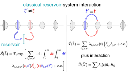
Fig. 1 shows the transition between a Langrangian-based dynamics to a Hamiltonian-based dynamics in the instantaneous limit. The Lagrangian framework incorporates the retarded response of the system; i.e. the action describes the effects on the system from the reservoir when there is a time lag between particle creation and annihilation at the system-reservoir interface. The reservoir removes particles with spin from site at time and reintroduces particles with spin at site at a later time , but the classical reservoir does not track the particle dynamics in the reservoir; usually we consider reservoirs that do not flip spins, so . Once is determined, we can calculate the thermal expectation value of physical observables of interest via:
| (2) | ||||
| (3) |
where is the time-dependent field describing the coupling between the reservoir and the system, is the chemical potential, is the electron number operator, is the time-ordering operator, and is the partition function.
There are two major challenges in evaluating . First, handling the time ordering is complex because the fields depend on two times, and . Second, the grand canonical formalism is required, because particle number is no longer conserved due to the interaction with the reservoir. The dimension increases from the canonical Hilbert-space dimension for electrons on sites, , to the full Hilbert-space dimension of for the system when a generic classical reservoir is incorporated.
The situation greatly simplifies by imposing an instantaneous-response limit on the classical reservoir, where both challenges described above disappear: (i) we can remain in a canonical formalism with fixed particle number and (ii) we can work with a Hamiltonian formalism, where time-ordering is easy to implement because all time-dependent object depend on only one time. The interaction between the system and the reservoir manifests as hopping terms, with the fields modulating the hopping strengths as shown in Fig. 1. Since the exponentials of hopping terms form a closed Lie group, they effectively act as modifying the single-particle basis. To engineer electron correlations, additional operators are required. We introduce on-site potential terms denoted by , where represents an additional set of time-dependent field; these fields allow for the creation of entanglement. By alternating between these terms in multiple layers, we construct the ansatz for a “time-evolution operator,” given by:
| (4) |
where is the initial state and is the number of layers (analogous to the number of time steps in time evolution). We omit as it can be absorbed into the and fields because only the product will be optimized.
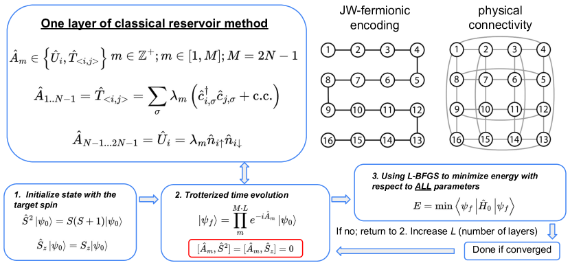
To make Eq. (4) more resource-efficient, three simplifications are applied to derive the final expression for the ansatz. First, the ansatz enforces the conservation of both the total spin and its -component, thereby reducing the optimization landscape to a smaller target spin subspace and eliminating concerns about spin contamination. This is achieved by pairing the spin-up and spin-down hopping terms, as previously shown in Ref. [37]. Consequently, the initial state must already have the target total spin and -component. For a total spin state with electrons distributed across sites (half filling), the configuration of the initial state is as follows: empty sites, doubly occupied sites, and spin-up occupied sites. See Appendix A for examples.
Second, we note that the aforementioned closure of the Lie algebra for the singles hopping terms is given by
| (5) |
where are site indices. This implies that including the hopping terms only along the Jordan-Wigner string will create indirect hopping terms between non adjacent sites. This closure property allows us to restrict the operator set to only adjacent hoppings along the Jordan-Wigner snake-like path, regardless of the system’s dimension or lattice connectivity. This reduces computational costs by avoiding the need for any Jordan–Wigner Pauli- string operators [38]. Consequently, the hopping part in the ansatz is further simplified to
| (6) |
where denotes adjacent sites along the 1D Jordan–Wigner snake-like path. Conceptually, this is akin to the compression algorithms for free fermionic systems discussed in Refs [39, 40].
Finally, we separate the hopping and potential terms for efficient implementation on a quantum computer. When separating the hopping terms, one can combine terms that commute into one exponent. In the case of an even number of sites, these terms are separated into two groups. The first group includes hopping terms with hopping indices such as , …, and so on, while the second group consists of terms such as , … , and so forth. Denoting the first hopping group as and the second hopping group as , we can rewrite the classical reservoir method ansatz as
| (7) | ||||
| (8) |
with being the parameter index of a set that combines all the terms in the ansatz. The whole classical reservoir method is summarized in Fig. 2 as a flow chart, outlining the process from state initialization and the ansatz expression in Eq. 8, as well as the fermionic encoding used to translate the problem onto quantum circuits via the Jordan-Wigner transformation. In detail, one layer contains a total of parameters, and each ansatz layer consists of three quantum circuit layers. We then perform optimizations on the and fields using noiseless energy measurements (optimization details are provided in Appendix B). At this point, the motivation for these approximations cannot be fully justified beyond their practical feasibility. However, the numerical results are robust and accurate.
III Numerical results
To quantify the accuracy of our results, we define the relative error as . We perform calculations on a two-dimensional periodic cluster [41], where each even-numbered site is connected to four neighboring odd-numbered sites, and vice versa, as illustrated in Fig. 3 (top panel). When studying two-dimensional systems, this model is interesting because it highlights the potential advantage of quantum computing, as it exhibits faster entanglement growth compared to the two-leg ladder system, which can typically be solved efficiently using DMRG classically [42]. For completeness, we also perform calculations on a two-leg ladder system to compare with the NP ansatz (details in Appendix C).
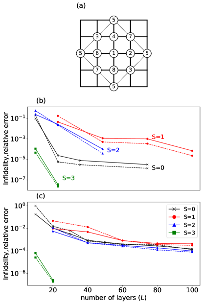
We can efficiently determine the ground state for different total spin values by starting with an initial state that has the target spin value. The performance for varying numbers of layers at each spin value is detailed in Fig. 3, panel (b). Naturally, we find that the difficulty of finding the ground state for different total spin values is directly related to the energy gap in each total spin sector (provided in Appendix D), with a smaller gap making it harder to find the ground state.
We also examine one case of the disordered Hubbard Hamiltonian. The hopping term in Eq. 1 is now given by , where , and represents a random number drawn from a normalized Gaussian distribution with mean zero and variance one. The on-site potential term is a random value drawn from the range . In Fig. 3, panel (c), it shows that the disorder does not significantly affect performance, demonstrating robustness against randomness.
IV Conclusion
We show that an instantaneous simplification of the classical reservoir, constrained to its instantaneous-response limit, can serve as an efficient method for ground-state preparation, offering a more feasible approach for near-term quantum computers.
In comparing this work to previous works, we find that the classical reservoir method produces an ansatz expression analogous to the NP ansatz; however, the motivation arises from cooling dynamics rather than the adiabatic theorem, which underpins the HVA. The classical reservoir method exploits total spin symmetry and a closure property of the Lie algebra in the Hubbard hopping terms. This allows the classical reservoir method to prepare a more accurate ground state in the strongly correlated regime, while also reducing implementation costs in the following ways:
-
1.
We only require the initial state to have the target total spin and do not need it to be the non-interacting ground state; it is most easily prepared by creating double occupancies in a single product state. The noininteracting state is more complicated to make in the position basis [33, 43], especially when it is degenerate [32].
-
2.
Constraining the system to a definite total spin as well as its -component allows us to find the ground state for each value of total spin easily and reduces the numerical cost by working within a smaller optimization landscape.
-
3.
The closure properties of the Lie algebra allow us to use a one-dimensional indexing scheme, eliminating the need for fermionic swap (fSWAP) gates [44] to handle nonadjacent vertical hopping terms in a two-dimensional system. This concept has also been introduced as the excitation-preserving (EP) ansatz in Ref. [35]. However, Ref. [35] reported that the EP ansatz often underperforms compared to the NP ansatz in two-dimensional systems. In contrast, we find that incorporating total spin into the consideration resolves this issue.
Using the classical reservoir method, we find high-accuracy results —infidelities reach the range of for 8- and 10-site two-dimensional systems, even in the strong correlation region ().
V Acknowledgment
This work was supported by the Department of Energy, Office of Basic Energy Sciences, Division of Materials Sciences and Engineering under grant no. DE-SC0023231. J.K.F. was also supported by the McDevitt bequest at Georgetown.
VI Data Availability
The data that support the findings of this article as well as the python code that run the calculations are openly available at [45].
References
- Kitaev et al. [2002] A. Y. Kitaev, A. Shen, and M. N. Vyalyi, Classical and quantum computation, 47 (American Mathematical Soc., 2002).
- Preskill [2018] J. Preskill, Quantum 2, 79 (2018).
- Varney et al. [2009] C. N. Varney, C.-R. Lee, Z. J. Bai, S. Chiesa, M. Jarrell, and R. T. Scalettar, Phys. Rev. B 80, 075116 (2009).
- Qin et al. [2016] M. Qin, H. Shi, and S. Zhang, Phys. Rev. B 94, 085103 (2016).
- Jiang et al. [2023] S. Jiang, D. J. Scalapino, and S. R. White, Phys. Rev. B 108, L161111 (2023).
- White [1992] S. R. White, Phys. Rev. Lett. 69, 2863 (1992).
- Troyer and Wiese [2005] M. Troyer and U.-J. Wiese, Phys. Rev. Lett. 94, 170201 (2005).
- LeBlanc et al. [2015] J. P. F. LeBlanc, A. E. Antipov, F. Becca, I. W. Bulik, G. K.-L. Chan, C.-M. Chung, Y. Deng, M. Ferrero, T. M. Henderson, C. A. Jiménez-Hoyos, E. Kozik, X.-W. Liu, A. J. Millis, N. V. Prokof’ev, M. Qin, G. E. Scuseria, H. Shi, B. V. Svistunov, L. F. Tocchio, I. S. Tupitsyn, S. R. White, S. Zhang, B.-X. Zheng, Z. Zhu, and E. Gull (Simons Collaboration on the Many-Electron Problem), Phys. Rev. X 5, 041041 (2015).
- Born and Fock [1928] M. Born and V. Fock, Z. Phys. 51, 165 (1928).
- Jansen et al. [2007] S. Jansen, M.-B. Ruskai, and R. Seiler, J. Math. Phys. 48, 102111 (2007).
- Farhi et al. [2000] E. Farhi, J. Goldstone, S. Gutmann, and M. Sipser, arXiv https://doi.org/10.48550/arXiv.quant-ph/0001106 (2000).
- Guéry-Odelin et al. [2019] D. Guéry-Odelin, A. Ruschhaupt, A. Kiely, E. Torrontegui, S. Martínez-Garaot, and J. G. Muga, Rev. Mod. Phys. 91, 045001 (2019).
- Hegade et al. [2021] N. N. Hegade, K. Paul, Y. Ding, M. Sanz, F. Albarrán-Arriagada, E. Solano, and X. Chen, Phys. Rev. Appl. 15, 024038 (2021).
- Demirplak and Rice [2003] M. Demirplak and S. A. Rice, J. Phys. Chem. A 107, 9937 (2003).
- Demirplak and Rice [2005] M. Demirplak and S. A. Rice, J. Phys. Chem. B 109, 6838 (2005).
- Berry [2009] M. V. Berry, J. Phys. A: Math. Theor. 42, 365303 (2009).
- Shor [1994] P. Shor, in Proceedings 35th Annual Symposium on Foundations of Computer Science (1994) pp. 124–134.
- Kitaev [1995] A. Y. Kitaev, arXiv https://doi.org/10.48550/arXiv.quant-ph/9511026 (1995).
- McClean et al. [2016] J. R. McClean, J. Romero, R. Babbush, and A. Aspuru-Guzik, New J. Phys. 18, 023023 (2016).
- Bharti et al. [2022] K. Bharti, A. Cervera-Lierta, T. H. Kyaw, T. Haug, S. Alperin-Lea, A. Anand, M. Degroote, H. Heimonen, J. S. Kottmann, T. Menke, W.-K. Mok, S. Sim, L.-C. Kwek, and A. Aspuru-Guzik, Rev. Mod. Phys. 94, 015004 (2022).
- Peruzzo et al. [2014] A. Peruzzo, J. McClean, P. Shadbolt, M.-H. Yung, X.-Q. Zhou, P. J. Love, A. Aspuru-Guzik, and J. L. O’brien, Nat. Commun 5, 4213 (2014).
- Cerezo et al. [2021] M. Cerezo, A. Arrasmith, R. Babbush, S. C. Benjamin, S. Endo, K. Fujii, J. R. McClean, K. Mitarai, X. Yuan, L. Cincio, and P. J. Coles, Nat. Rev. Phys. 3, 625 (2021).
- Grimsley et al. [2019] H. R. Grimsley, S. E. Economou, E. Barnes, and N. J. Mayhall, Nat. Commun 10, 3007 (2019).
- Gyawali and Lawler [2022] G. Gyawali and M. J. Lawler, Phys. Rev. A 105, 012413 (2022).
- Burton et al. [2023] H. G. Burton, D. Marti-Dafcik, D. P. Tew, and D. J. Wales, Npj Quantum Inf. 9, 75 (2023).
- Larsen et al. [2024] J. B. Larsen, M. D. Grace, A. D. Baczewski, and A. B. Magann, Phys. Rev. Res. 6, 033336 (2024).
- Magann et al. [2022] A. B. Magann, K. M. Rudinger, M. D. Grace, and M. Sarovar, Phys. Rev. Lett. 129, 250502 (2022).
- Xie et al. [2022] Q. Xie, K. Seki, and S. Yunoki, Phys. Rev. B 106, 155153 (2022).
- Claeys et al. [2019] P. W. Claeys, M. Pandey, D. Sels, and A. Polkovnikov, Phys. Rev. Lett. 123, 090602 (2019).
- Marti et al. [2024] L. Marti, R. Mansuroglu, and M. J. Hartmann, arXiv preprint https://doi.org/10.48550/arXiv.2403.14506 (2024).
- Reiner et al. [2019] J.-M. Reiner, F. Wilhelm-Mauch, G. Schön, and M. Marthaler, QST 4, 035005 (2019).
- Wecker et al. [2015] D. Wecker, M. B. Hastings, and M. Troyer, Phys. Rev. A 92, 042303 (2015).
- Cade et al. [2020] C. Cade, L. Mineh, A. Montanaro, and S. Stanisic, Phys. Rev. B 102, 235122 (2020).
- Cai [2020] Z. Cai, Phys. Rev. Appl. 14, 014059 (2020).
- Alvertis et al. [2024] A. M. Alvertis, A. Khan, T. Iadecola, P. P. Orth, and N. Tubman, arXiv preprint https://doi.org/10.48550/arXiv.2408.00836 (2024).
- Breuer and Petruccione [2002] H.-P. Breuer and F. Petruccione, The theory of open quantum systems (Oxford University Press, USA, 2002).
- Izmaylov et al. [2020] A. F. Izmaylov, M. Díaz-Tinoco, and R. A. Lang, Phys. Chem. Chem. 22, 12980 (2020).
- Jordan and Wigner [1928] P. Jordan and E. Wigner, Zeitschrift für Physik 47, 631 (1928).
- Kökcü et al. [2022] E. Kökcü, D. Camps, L. Bassman Oftelie, J. K. Freericks, W. A. de Jong, R. Van Beeumen, and A. F. Kemper, Phys. Rev. A. 105, 032420 (2022).
- Kökcü et al. [2023] E. Kökcü, D. Camps, L. B. Oftelie, W. A. de Jong, R. V. Beeumen, and A. F. Kemper, arXiv preprint arXiv.2303.09538 (2023).
- Betts et al. [1996] D. Betts, S. Masui, N. Vats, and G. Stewart, Can. J. Phys. 74, 54 (1996).
- Noack et al. [1996] R. Noack, S. White, and D. Scalapino, Physica C: Superconductivity 270, 281 (1996).
- Jiang et al. [2018] Z. Jiang, K. J. Sung, K. Kechedzhi, V. N. Smelyanskiy, and S. Boixo, Phys. Rev. Appl. 9, 044036 (2018).
- Verstraete et al. [2009] F. Verstraete, J. I. Cirac, and J. I. Latorre, Phys. Rev. A 79, 032316 (2009).
- Z.He [2025] J. K. F. Z.He, A. F. Kemper, Dataset (2025).
- Paszke et al. [2017] A. Paszke, S. Gross, S. Chintala, G. Chanan, E. Yang, Z. DeVito, Z. Lin, A. Desmaison, L. Antiga, and A. Lerer, (2017).
- Chen et al. [2021] J. Chen, H.-P. Cheng, and J. K. Freericks, J. Chem. Theory Comput. 17, 841 (2021).
Appendix A Initial state examples
The only requirement for the initial state is to have the target spin value. But, we find it is advantageous to intersperse the doubly occupied sites and the empty sites. Hence, we select the simplest states that fulfill this requirement, which is a product state. We illustrate this with an eight-site example.
For the sector, the choice is as follows:
| (A1) |
For nonzero sector initial states, we work with states that have . We assign double occupancies to lattice sites, with the remaining electrons being spin-up on sites, leaving empty sites. For example, for the sector, a possible starting state is
| (A2) |
Appendix B Numerical optimization details
We use the L-BFGS algorithm from the GPU-supported PyTorch package for optimization [46]. The parameter amplitudes are initialized as random values within the range . Since we lack prior knowledge about the optimal amplitude values, one might consider initializing them all to zero. However, we found that this approach leads to numerical instability. By choosing a small random initialization, we ensure numerical stability while keeping the values small enough to most likely avoid divergence in the optimized energy.
Though our goal is to implement this algorithm on a quantum computer, we are currently using classical computer simulations. For the exponential of the hopping terms, we use an SU(2) identity [47] to implement the hopping terms instead of directly calculating the matrix exponential, which speeds up the computation. This is given by
| (B1) |
The stopping threshold for the optimization in this work is set to a gradient norm smaller than 0.001.
Appendix C Two leg ladder system
In Fig. C1, we present numerical results for and ladders in both the weakly and strongly correlated regimes. Note that the ground-state total spin at depends on the number of sites . Specifically, it is a singlet for (e.g., ) and a triplet for (e.g., ) [32]. In the case of a weakly correlated region (), when compared on a linear-connectivity quantum machine, no clear pattern emerges. In the system, the NP ansatz [33] requires 432 parameters and a circuit depth of 48 to achieve a fidelity of 0.99, while this work requires 475 parameters and a circuit depth of 75 to reach a fidelity of 0.95 (with an relative error of 0.01). In the system, however, this work performs better, achieving a fidelity of 0.99 with 150 parameters and a circuit depth of 30, whereas the NP ansatz [33] requires 392 parameters and a circuit depth of 56 to achieve the same fidelity.
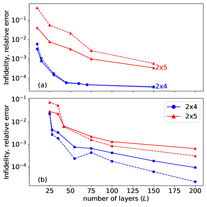
From the ladder system data, this method offers two key improvements. First, in the strong correlation regime (), subsequent work on the NP ansatz [35] reported that the largest system investigated, a lattice with open boundary conditions, achieved a relative error (defined as ) that mostly saturates around 0.01. In contrast, for the largest system studied here—a ladder system—we achieve higher accuracy, with a similarly defined relative error (given by ) of 0.001 when .
Second, this work demonstrates a potential pathway (employing a one-dimensional indexing scheme) for efficiently simulating multi-dimensional systems that were previously considered unsatisfactory [35]. An intriguing observation arises when comparing the ladder system to a two-dimensional periodic cluster. The latter, with increased site connectivity, surprisingly yields better results. This indicates that the classical reservoir approach can be well-suited for simulating realistic three-dimensional lattices with higher connectivity.
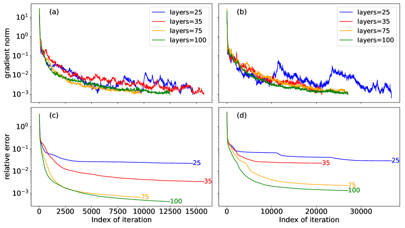
Additionally, in Fig. C2, we provide details of the convergence and the number of iterations required as the system size increases. We present results for only, as the total spin value of the ground state differs in the region for the and systems, which can affect performance. The results show that optimization can reduce the relative error to below 0.01 relatively quickly, typically within a few thousand iterations for both system sizes. However, achieving the next order of accuracy, 0.001, often requires 5–7 times more iterations, as the step size along the gradient direction becomes very small when the optimization approaches the local minimum.
Appendix D energy gap table
In Table 1, we provide the energy gap values for the two-dimensional periodic cluster [41] for both the standard and disordered Hubbard Hamiltonians studied in work.
| standard | 1.12945 | 0.62746 | 0.78693 | 1.63385 |
| disordered | 0.56782 | 0.16508 | 0.32210 | 2.12290 |
For the standard Hubbard Hamiltonian, the total spin values corresponding to each energy gap are ranked from largest to smallest as follows: , , , and . This ordering corresponds to the observed difficulty of obtaining the ground state in each total spin sector, as seen in Fig. 3.
Similarly, in the disordered Hubbard Hamiltonian, we observe the same pattern, where the difficulty of finding the ground state is inversely related to the energy gap.