Systolic $S^{1}$-index and characterization of non-smooth Zoll convex bodies

Abstract.

We define the systolic $S^{1}$-index of a convex body as the Fadell–Rabinowitz index of the space of centralized generalized systoles associated with its boundary. We show that this index is a symplectic invariant. Using the systolic $S^{1}$-index, we propose a definition of generalized Zoll convex bodies and prove that this definition is equivalent to the usual one in the smooth setting. Moreover, we show how generalized Zoll convex bodies can be characterized in terms of their Gutt–Hutchings capacities and we prove that the space of generalized Zoll convex bodies is closed in the space of all convex bodies. As a corollary, we establish that if the interior of a convex body is symplectomorphic to the interior of a ball, then such a convex body must be generalized Zoll, and in particular Zoll if its boundary is smooth. Finally, we discuss some examples.

1 Introduction

We say that $C\subset\mathbb{R}^{2n}$ is a convex body if $C$ is the closure of a bounded open convex set. The boundary of such a set is a hypersurface,which is a Lipschitz submanifold of $\mathbb{R}^{2n}$ and, as such, has a tangent plane and an outer normal vector that are defined almost everywhere. Moreover, we can define the tangent cone and the normal cone at every point of $\partial C$ (see [Cla83]).

We define the outward normal cone of $\partial C$ at $x\in\partial C$ as

$$N_{\partial C}(x)=\{\eta\in\mathbb{R}^{2n}\backslash\{0\}\mid\langle\eta,x-y\rangle\geq 0,\quad\forall y\in C\}.$$

If $\partial C$ is differentiable at $x$, then $N_{\partial C}(x)=\mathbb{R}_{+}n$, where $n$ is the unit outer normal vector at $x$. Let $J_{0}$ denote the standard complex structure of $\mathbb{R}^{2n}$, and let $\mathbb{T}:=\mathbb{R}/\mathbb{Z}$.

Following [Cla81], we define the set of generalized closed characteristics on $\partial C$, denoted by $\operatorname{Char}(\partial C)$, as the set

$$\operatorname{Char}(\partial C):=\{\gamma:\mathbb{T}\to\partial C\mid\dot{\gamma}(t)\in J_{0}N_{\partial C}(\gamma(t)),\ \text{a.e.}\}/\sim,$$

where $\gamma:\mathbb{T}\to\partial C$ is an absolutely continuous loop satisfying the condition that there exist positive constants $m_{\gamma},M_{\gamma}>0$ such that

$$m_{\gamma}\leq|\dot{\gamma}(t)|\leq M_{\gamma},\quad\text{a.e.}$$

The equivalence relation $\sim$ is defined as follows. We say that $\gamma_{1}$ is equivalent to $\gamma_{2}$ (i.e., $\gamma_{1}\sim\gamma_{2}$) if there exists a bi-Lipschitz homeomorphism $\tau:\mathbb{T}\to\mathbb{T}$ such that $\tau(0)=0$ and $\gamma_{1}(t)=\gamma_{2}(\tau(t)).$ This homeomorphism must preserve orientation. Let $\gamma:\mathbb{T}\to\mathbb{R}^{2n}$ be an absolutely continuous loop. We define the action of $\gamma$ as

$$\mathcal{A}(\gamma):=\int\limits_{\gamma}\lambda=\frac{1}{2}\int\limits_{\mathbb{T}}\langle\dot{\gamma}(t),J_{0}\gamma(t)\rangle\,dt,$$

where $\lambda$ is any primitive 1-form of the standard symplectic form

$$\omega_{0}=\sum_{j=1}^{n}dx_{j}\wedge dy_{j}.$$

From Stokes’ formula, it follows that the action is invariant under reparametrizations that preserve orientation. Thus, the action is well-defined on the space $\operatorname{Char}(\partial C)$, is finite, and can easily be shown to be positive for every element of $\operatorname{Char}(\partial C)$. The subset of $\operatorname{Char}(\partial C)$ consisting of generalized closed characteristics with minimal action is denoted by $\operatorname{Sys}(\partial C)$, and it is always non-empty (see [Cla81, AO14]). Elements of this set are called generalized systoles. To introduce an $S^{1}$-action on the spaces $\operatorname{Char}(\partial C)$ and $\operatorname{Sys}(\partial C)$, we need a choice of parametrization.

Assuming the origin is contained in the interior of $C$, we can define a positively $2$-homogeneous function $H_{C}:\mathbb{R}^{2n}\to\mathbb{R}$ such that $H_{C}^{-1}(1)=\partial C$. Since $H_{C}$ is convex, the subdifferential of $H_{C}$ at $x$ is defined for every $x\in\mathbb{R}^{2n}$ as

$$\partial H_{C}(x)=\{\eta\in\mathbb{R}^{2n}\mid H_{C}(y)-H_{C}(x)\geq\langle\eta,y-x\rangle,\quad\forall y\in\mathbb{R}^{2n}\}.$$

For every $x\in\mathbb{R}^{2n}$, the set $\partial H_{C}(x)$ is a non-empty convex compact set, which is precisely $\{\nabla H_{C}(x)\}$ when $H_{C}$ is differentiable at $x$. Moreover, the multifunction $\partial H_{C}$ is upper semi-continuous. See [Cla83] for the proof of these properties.

The function $H_{C}$ allows us to define generalized closed characteristics on $\partial C$ as follows:

$$\operatorname{Char}(\partial C)=\left\{\gamma:\mathbb{T}\to\partial C\text{ absolutely continuous}\mid\dot{\gamma}(t)\in TJ_{0}\partial H_{C}(\gamma(t))\ \text{a.e.},\ \text{for some }T>0\right\}.$$

This definition is equivalent to the previous one in the set-theoretic sense. Indeed, any $\gamma\in\operatorname{Char}(\partial C)$, according to this definition, has a derivative that is bounded both from below and above. Moreover, $N_{\partial C}(x)=\mathbb{R}_{+}\partial H_{C}(x)$ for all $x\in\partial C$. Hence, the conclusion follows.

In addition, generalized closed characteristics with a fixed action $T>0$ are precisely the generalized closed characteristics satisfying the equation

$$\dot{\gamma}(t)\in TJ_{0}\partial H_{C}(\gamma(t)),\quad\text{a.e.}$$

This follows from the fact that $2$-homogeneity of $H_{C}$ implies that

$$H_{C}(x)=\frac{1}{2}\langle\partial H_{C}(x),x\rangle,\quad x\in\mathbb{R}^{2n},$$

where the equality holds in the set-theoretic sense (for any element in the corresponding subdifferential). Consequently, for $\gamma\in\operatorname{Char}(\partial C)$ such that

$$\dot{\gamma}(t)\in TJ_{0}\partial H_{C}(\gamma(t)),\quad\text{a.e.},$$

it holds that $\mathcal{A}(\gamma)=T$.

On the space $\operatorname{Char}(\partial C)$, we now have a natural $S^{1}$-action given by:

$$\theta\cdot\gamma=\gamma(\cdot-\theta),\quad\theta\in\mathbb{T},\ \gamma\in\operatorname{Char}(\partial C).$$

Since the action of an absolutely continuous loop $\gamma:\mathbb{T}\to\mathbb{R}^{2n}$ remains invariant under the $S^{1}$-action, it follows that the subsets of generalized closed characteristics with a fixed action are $S^{1}$-invariant sets. In particular, $\operatorname{Sys}(\partial C)$ is $S^{1}$-invariant.

Let

$$\pi_{0}(\gamma)=\gamma-\int\limits_{\mathbb{T}}\gamma(t)\,dt$$

denote the orthogonal $L^{2}$-projection onto the space of closed curves in $\mathbb{R}^{2n}$ with zero mean.

We define the set of centralized generalized systoles, denoted by $\operatorname{Sys}_{0}(\partial C)$, as

$$\operatorname{Sys}_{0}(\partial C):=\pi_{0}(\operatorname{Sys}(\partial C))=\{\pi_{0}(\gamma)\mid\gamma\in\operatorname{Sys}(\partial C)\}.$$

Since $\partial H_{C}$ is bounded on $\partial C$, it follows that the spaces $\operatorname{Sys}(\partial C)$ and $\operatorname{Sys}_{0}(\partial C)$ are uniformly bounded in the $W^{1,\infty}$-norm. We endow the spaces $\operatorname{Sys}(\partial C)$ and $\operatorname{Sys}_{0}(\partial C)$ with the compact-open topology (i.e., $C^{0}$-topology). As shown in Proposition 2.1, these spaces are compact with respect to this topology, which is actually equivalent to the weak^∗ topology of $W^{1,\infty}$. In contrast, with respect to other topologies, such as the strong topology of $W^{1,1}$, these spaces are, in general, not compact (see Proposition 2.2). Hence, the uniform norm is natural for studying these spaces if one aims to retain compactness properties, as in the smooth setting.

Consider the map

$$\pi_{0}:\operatorname{Sys}(\partial C)\to\operatorname{Sys}_{0}(\partial C).$$

This map is generally an $S^{1}$-equivariant convex fibration, which means that $\pi_{0}$ is a continuous, $S^{1}$-equivariant surjection, and for every $\gamma_{0}\in\operatorname{Sys}_{0}(\partial C)$, the preimage $\pi_{0}^{-1}(\gamma_{0})$ is a convex, compact set (see claim (1) of Proposition 2.3). Moreover, statement (2) of Proposition 2.3 asserts that if $C$ is strictly convex, meaning that for any $x,y\in C$, the set $[x,y]\setminus\{x,y\}$ lies entirely within $\text{int}(C)$, then $\pi_{0}$ is an $S^{1}$-equivariant homeomorphism. In the general case, even in the smooth category, $\pi_{0}$ is not injective (see Example 2.4).

Fadell-Rabinowitz index

Let $\mathbb{F}$ denote a field, and consider a paracompact topological space $X$ that has an $S^{1}$-action. In accordance with Borel’s framework, we define the $S^{1}$-equivariant cohomology with coefficients in $\mathbb{F}$ as

$$\operatorname{H}^{*}_{S^{1}}(X;\mathbb{F})=\operatorname{H}^{*}(X\times_{S^{1}}ES^{1};\mathbb{F}),$$

where $ES^{1}\to BS^{1}$ represents the universal $S^{1}$-bundle over the classifying space, and

$$X\times_{S^{1}}ES^{1}:=(X\times ES^{1})/S^{1}.$$

For example, we can select $ES^{1}:=S^{\infty}\subset\mathbb{C}^{\infty}$ and $BS^{1}:=\mathbb{C}P^{\infty}$. The cohomology of the classifying space $BS^{1}$ is given by the ring $\operatorname{H}^{*}(BS^{1};\mathbb{F})\cong\mathbb{F}[e_{B}]$, where $e_{B}$ is a generator of $\operatorname{H}^{2}(BS^{1};\mathbb{F})$. The projection map $\pi_{2}:X\times_{S^{1}}ES^{1}\to BS^{1}$, specified by $\pi_{2}([x,y])=[y]$, induces a homomorphism of cohomology rings given by

$$\pi^{*}_{2}:\operatorname{H}^{*}(BS^{1};\mathbb{F})\to\operatorname{H}^{*}_{S^{1}}(X;\mathbb{F}).$$

We denote $e:=\pi_{2}^{*}e_{B}$ as the fundamental class associated with the $S^{1}$-space $X$. The Fadell-Rabinowitz index for the space $X$ is defined as

$$\operatorname{ind}_{\operatorname{FR}}(X;\mathbb{F})=\sup_{k\geq 0}\{k+1\mid e^{k}\neq 0\}.$$

Additionally, we define $\operatorname{ind}_{\operatorname{FR}}(\emptyset;\mathbb{F})=0$.

We will focus on the case where $\mathbb{F}=\mathbb{Z}_{2}$, following the results in [Mat24]. Nevertheless, analogous results to those in this paper hold for any field, as [Mat24, Theorem A] can be established for arbitrary fields.

Definition 1.1.

Let $C\subset\mathbb{R}^{2n}$ be a convex body, and let $C^{\prime}$ be any translation of $C$ whose interior contains the origin. We define the systolic $S^{1}$-index of $C$ as

$$\operatorname{ind}_{\operatorname{sys}}^{S^{1}}(C)=\operatorname{ind}_{\operatorname{FR}}(\operatorname{Sys}_{0}(\partial C^{\prime})),$$

where the topology on $\operatorname{Sys}_{0}(\partial C^{\prime})$ is induced by the uniform norm.

As the notation suggests, this definition does not depend on the choice of the translation $C^{\prime}$. This is a consequence of Theorem 1.2 below.

In [GH18], Gutt and Hutchings defined a monotone sequence of capacities $c_{k}^{GH}$ for the class of Liouville domains. As shown in [Mat24, Theorem A], for convex bodies, the Gutt–Hutchings capacities coincide with the spectral invariants introduced by Ekeland and Hofer in [EH87].

Using this result, we prove the following.

Theorem 1.2.

Let $C\subset\mathbb{R}^{2n}$ be a convex body whose interior contains the origin. Then, it holds that

$$\operatorname{ind}_{\operatorname{FR}}(\operatorname{Sys}_{0}(\partial C))=\max\{k\in\mathbb{N}\mid c_{k}^{GH}(C)=c_{1}^{GH}(C)\}.$$

Moreover, if $C$ is strictly convex or $\partial C$ is smooth, we have

$$\operatorname{ind}_{\operatorname{FR}}(\operatorname{Sys}_{0}(\partial C))=\operatorname{ind}_{\operatorname{FR}}(\operatorname{Sys}(\partial C)).$$

In particular, $\operatorname{ind}_{\operatorname{sys}}^{S^{1}}(C)$ is well-defined for a convex body $C\subset\mathbb{R}^{2n}$, and it holds

$$\operatorname{ind}_{\operatorname{sys}}^{S^{1}}(C)=\max\{k\in\mathbb{N}\mid c_{k}^{GH}(C)=c_{1}^{GH}(C)\}.$$

Since $c_{k}^{GH}(C)\to\infty$ as $k\to\infty$, it follows that $\operatorname{ind}_{\operatorname{sys}}^{S^{1}}(C)$ is finite. Moreover, from the previous theorem, we obtain the following immediate corollary.

Corollary 1.3.

The systolic $S^{1}$-index of convex bodies is a symplectic invariant. More precisely, if the interior of a convex body $C_{1}$ is symplectomorphic to the interior of a convex body $C_{2}$, then

$$\operatorname{ind}_{\operatorname{sys}}^{S^{1}}(C_{1})=\operatorname{ind}_{\operatorname{sys}}^{S^{1}}(C_{2}).$$

Remark.

From Theorem 1.2 and [GR24, Theorem 1.2], we deduce that

$$\operatorname{ind}_{\operatorname{sys}}^{S^{1}}(C)=\max\{k\in\mathbb{N}\mid c_{k}^{EH}(C)=c_{1}^{EH}(C)\},$$

where $c_{k}^{EH}$ denotes the Ekeland–Hofer capacities introduced in [EH90].

Let $\operatorname{Conv}(\mathbb{R}^{2n})$ denote the set of all convex bodies endowed with the Hausdorff-distance topology. Since $\operatorname{ind}_{\operatorname{sys}}^{S^{1}}$ is finite for every convex body, the function

$$\operatorname{ind}_{\operatorname{sys}}^{S^{1}}:\operatorname{Conv}(\mathbb{R}^{2n})\to\mathbb{N}$$

is well-defined. Moreover, the function is upper semicontinuous and uniformly bounded.

The upper semicontinuity of $\operatorname{ind}_{\operatorname{sys}}^{S^{1}}$ is a straightforward corollary of the previous theorem (see claim (1) of Proposition 3.3.1). The existence of a uniform bound follows from the existence of the Loewner–Behrend–John ellipsoid (see [Joh48] or [Vit00, Appendix B]). Indeed, using this ellipsoid, we obtain explicit bounds (see claim (2) of Proposition 3.3.1):

• For every $C\in\operatorname{Conv}(\mathbb{R}^{2n})$, we have $\operatorname{ind}_{\operatorname{sys}}^{S^{1}}(C)\leq 4n^{3}$. If $C=-C$, then $\operatorname{ind}_{\operatorname{sys}}^{S^{1}}(C)\leq 2n^{2}$.

Now, consider the standard $S^{1}$-action on $\mathbb{C}^{n}$ given by:

$$\theta\cdot z=e^{2\pi i\theta}z,\quad\theta\in\mathbb{T},\ z\in\mathbb{C}^{n}.$$

We say that $C\in\operatorname{Conv}(\mathbb{R}^{2n})$ is $S^{1}$-invariant if, for every $\theta\in\mathbb{T}$, it holds that

$$\theta\cdot C=C.$$

For the $S^{1}$-invariant category and the smooth category of convex bodies, we have better estimates:

• For every $C\in\operatorname{Conv}(\mathbb{R}^{2n})$ such that $C$ is $S^{1}$-invariant, it holds that $\operatorname{ind}_{\operatorname{sys}}^{S^{1}}(C)\leq n$.

• For every $C\in\operatorname{Conv}(\mathbb{R}^{2n})$ with a smooth boundary, it holds that $\operatorname{ind}_{\operatorname{sys}}^{S^{1}}(C)\leq n$.

The estimate for the $S^{1}$-invariant case follows from claim (3) of Proposition 3.3.1. The estimate in the smooth case follows from Corollary 4.1.1. Since a ball in $\mathbb{R}^{2n}$ has the systolic $S^{1}$-index $n$, it follows that the estimates in the $S^{1}$-invariant and smooth categories are optimal.

Let $C\subset\mathbb{R}^{2n}$ be a convex body with a smooth boundary that is transverse to all lines through the origin (note that this is equivalent to the condition that the origin is contained in $\text{int}(C)$). For such a convex body, $(C,\lambda_{0})$ is a Liouville domain, where

$$\lambda_{0}=\frac{1}{2}\sum_{j=1}^{n}(x_{j}\,dy_{j}-y_{j}\,dx_{j})$$

is the standard Liouville form, which is a primitive of the standard symplectic form $\omega_{0}$.

The Reeb vector field $R$ is defined on $\partial C$ by the system of equations:

$$i_{R}\lambda_{0}=1,\quad i_{R}\omega_{0}=0.$$

A convex body $C$ with a smooth boundary is called Zoll if all of its Reeb orbits are closed and share a common minimal period.

Considering the established properties of the systolic $S^{1}$-index, we propose the following definition.

Definition 1.4.

A convex body $C\subset\mathbb{R}^{2n}$ is a generalized Zoll convex body if it satisfies

$$\operatorname{ind}_{\operatorname{sys}}^{S^{1}}(C)\geq n.$$

This definition is inspired by the work of Ginzburg, Gürel, and Mazzucchelli [GGM21] and [Mat24]. From [Mat24, Corollary B.2], it follows that a smooth and strongly convex body $C$ (i.e., one whose boundary $\partial C$ has positive sectional curvature everywhere) is Zoll if and only if $c^{GH}_{1}(C)=c^{GH}_{n}(C)$. The next theorem shows that the assumption of strong convexity can be dropped and that the characterization using Gutt-Hutchings capacities still holds for generalized Zoll convex bodies.

Theorem 1.5.

The following statements hold:

1. A convex body $C$ is generalized Zoll if and only if $c^{GH}_{1}(C)=c^{GH}_{n}(C)$.

2. A convex body $C$ with a smooth boundary is generalized Zoll if and only if it is Zoll.

3. The space of generalized Zoll convex bodies is closed in the space of all convex bodies with respect to the Hausdorff distance topology.

Statement (2) of this theorem justifies the term "generalized Zoll convex body." Additionally, we have the following immediate corollary.

Corollary 1.6.

If the interior of a convex body $C\subset\mathbb{R}^{2n}$ is symplectomorphic to the interior of a ball, then $C$ is a generalized Zoll convex body. In particular, if the boundary of $C$ is smooth, then $C$ is Zoll.

So far, the only examples of generalized Zoll convex bodies that are not Zoll in the usual sense come from non-smooth convex bodies whose interior is symplectomorphic to the interior of a ball (see [Tra95, Sch05, LMS13, Rud22]). One such example is the Lagrangian product of the unit ball in the $\|\cdot\|_{\infty}$-norm and the unit ball in the $\|\cdot\|_{1}$-norm, which we denote by $B_{\infty}\times B_{1}$. In Example 4.2.3, we show that $B_{\infty}\times B_{1}$ is generalized Zoll without using the fact that its interior is symplectomorphic to a ball.

We define the evaluation map

$$\text{ev}_{0}:(\operatorname{Sys}(\partial C),\|\cdot\|_{\infty})\to(\partial C,|\cdot|),\quad\text{ev}_{0}(\gamma)=\gamma(0).$$

This map is continuous.

If $C\subset\mathbb{R}^{2n}$ is a convex body with a smooth boundary whose interior contains the origin, it holds that $C$ is generalized Zoll if and only if $\text{ev}_{0}(\operatorname{Sys}(\partial C))=\partial C$. This is no longer true in the non-smooth case. In particular, the condition $\text{ev}_{0}(\operatorname{Sys}(\partial C))=\partial C$ is not sufficient (see Example 4.2.1 of the polydisc). However, under stronger assumptions, $\text{ev}_{0}$ can provide a sufficient condition for a convex body to be a generalized Zoll (see Proposition 4.2.2). As shown in Example 4.2.3, $B_{\infty}\times B_{1}$ is a non-smooth generalized Zoll convex body that satisfies the condition of Proposition 4.2.2. In particular, we have $\text{ev}_{0}(\operatorname{Sys}(\partial(B_{\infty}\times B_{1})))=\partial(B_{\infty}\times B_{1})$.

We conclude this introduction with a list of some open questions.

Question 1.

Is there a continuous $S^{1}$-equivariant map $s:\operatorname{Sys}_{0}(\partial C)\to\operatorname{Sys}(\partial C)$, possibly a section of $\pi_{0}$, i.e., a map $s$ such that $\pi_{0}\circ s=\text{id}$? In particular, does it always hold that $\operatorname{ind}_{\operatorname{FR}}(\operatorname{Sys}_{0}(\partial C))=\operatorname{ind}_{\operatorname{FR}}(\operatorname{Sys}(\partial C))$?

Question 2.

What is the global maximum of the function $\operatorname{ind}_{\operatorname{sys}}^{S^{1}}:\operatorname{Conv}(\mathbb{R}^{2n})\to\mathbb{N}$? Does it hold that for every convex body $C\subset\mathbb{R}^{2n}$, $\operatorname{ind}_{\operatorname{sys}}^{S^{1}}(C)\leq n$?

Question 3.

If $C$ is a generalized Zoll convex body, does it hold that $\text{ev}_{0}(\operatorname{Sys}(\partial C))=\partial C$? Is the converse true if $\operatorname{Sys}(\partial C)$ is connected?

Question 4.

If $C\subset\mathbb{R}^{2n}$ is a generalized Zoll convex body, is it true that the spaces $\operatorname{Sys}(\partial C)$ and $\operatorname{Sys}_{0}(\partial C)$ have the homology type of a sphere $S^{2n-1}$?

Question 5.

What is the form of Gutt-Hutchings capacities for $k>n$ for generalized Zoll convex bodies (see [MR23] for the answer in a smooth strongly convex case)?

Question 6.

Are there exotic generalized Zoll convex bodies, i.e., those with a systolic ratio different from that of a ball? In particular, are there generalized Zoll convex bodies that do not belong to the Hausdorff closure of the space of smooth Zoll convex bodies?

Question 7.

Are generalized Zoll convex bodies local maximizers of the systolic ratio in the space of convex bodies with respect to the Hausdorff distance topology, whether in general or in the centrally symmetric case (see [AB23, ABE23] for the partial results in the smooth setting)?

Acknowledgements. I would like to express my gratitude to my advisor, Alberto Abbondandolo, for his invaluable guidance and support throughout my PhD studies. I would also like to thank Souheib Allout for several valuable discussions.

This project is supported by the SFB/TRR 191 ‘Symplectic Structures in Geometry, Algebra and Dynamics,’ funded by the DFG (Projektnummer 281071066 - TRR 191).

2 Spaces of generalized and centralized generalized systoles

In this section, we consider the problem of choosing a natural topology on the spaces $\operatorname{Sys}(\partial C)$ and $\operatorname{Sys}_{0}(\partial C)$, as well as relation between these spaces. First, we recall some classical results from convex analysis.

Let $f:\mathbb{R}^{m}\to\mathbb{R}$ be a convex function. Such a function is locally Lipschitz continuous. Moreover, the directional derivative

$$f^{\prime}(x;v):=\lim_{t\downarrow 0}\frac{f(x+tv)-f(x)}{t}$$

is finite for every $x\in\mathbb{R}^{m}$ and $v\in\mathbb{R}^{m}$.

The function $f^{\prime}(x;\cdot)$ is positively homogeneous, subadditive, and Lipschitz continuous. Additionally, the function $f^{\prime}$ is upper semicontinuous as a function of $(x,v)$.

Let $\langle\cdot,\cdot\rangle$ denote the standard scalar product. We can express the subdifferential of $f$ at $x$, denoted by $\partial f(x)$, as

$$\partial f(x):=\{\xi\in\mathbb{R}^{m}\mid f^{\prime}(x,v)\geq\langle\xi,v\rangle,\quad\forall v\in\mathbb{R}^{m}\}.$$

The set $\partial f(x)$ is a non-empty, convex, and compact subset of $\mathbb{R}^{m}$. Moreover, $f^{\prime}(x;\cdot)$ is the support function of $\partial f(x)$, and therefore it holds that

$$f^{\prime}(x;v)=\max\{\langle v,\xi\rangle\mid\xi\in\partial f(x)\}.$$

For more details on these results, we refer the reader to [Cla83].

The next proposition is part of the general compactness theory for weak solutions of differential equations, as presented in [Cla83, Theorem 3.1.7]. For completeness, we provide a self-contained proof here.

Proposition 2.1.

Let $C\subset\mathbb{R}^{2n}$ be a convex body whose interior contains the origin. On the spaces $\operatorname{Sys}(\partial C)$ and $\operatorname{Sys}_{0}(\partial C)$, the compact-open topology and weak^∗-$W^{1,\infty}$ topology are equivalent. Moreover, the spaces $\operatorname{Sys}(\partial C)$ and $\operatorname{Sys}_{0}(\partial C)$ are compact in this topology.

Proof.

Let $C$ be a convex body whose interior contains the origin. We can assume without loss of generality that the action on the space of generalized systoles is $1$. Then $\gamma\in\operatorname{Sys}(\partial C)$ if and only if $\gamma:\mathbb{T}\to\partial C$ is Lipschitz and satisfies the weak equation

$$\dot{\gamma}(t)\in J_{0}\partial H_{C}(\gamma(t)),\quad\text{a.e.}$$ (2.1)

This equation is equivalent to the condition that

$$H_{C}^{\prime}(\gamma(t);v)+\langle J_{0}\dot{\gamma}(t),v\rangle\geq 0,\quad\forall v\in\mathbb{R}^{2n}$$ (2.2)

holds for almost every $t\in\mathbb{T}$, due to the relation between the subdifferential and the directional derivative. From (2.1) and the fact that $\partial H_{C}$ is bounded on $\partial C$, we get that the space $\operatorname{Sys}(\partial C)$ is uniformly bounded in the $W^{1,\infty}$-norm. Therefore, if $\gamma_{k}\in\operatorname{Sys}(\partial C)$ is an arbitrary sequence, it has a convergent subsequence in the weak^∗-$W^{1,\infty}$ topology. Weak^∗-$W^{1,\infty}$ topology convergence implies uniform convergence (by Arzelà-Ascoli), and therefore we can assume that $\gamma_{k}$ converges to some $\gamma$ uniformly and in the weak^∗-$W^{1,\infty}$ topology (we will keep the same notation for the subsequence). Since $\partial C$ is compact, we conclude that $\gamma:\mathbb{T}\to\partial C$. Moreover, the uniform $W^{1,\infty}$-bound on $\operatorname{Sys}(\partial C)$ implies that $\gamma$ is Lipschitz. Now we need to show that $\gamma$ is a solution of equation (2.1).

Let $U\subset\mathbb{T}$ be any measurable subset. From the reformulation of (2.1) given by (2.2), we have that

$$\int_{U}\left(H_{C}^{\prime}(\gamma_{k}(t);v)+\langle J_{0}\dot{\gamma}_{k}(t),v\rangle\right)\,dt\geq 0.$$

By the upper semi-continuity of $H_{C}^{\prime}$ and the uniform and weak^∗-$W^{1,\infty}$ convergence of $\gamma_{k}$, the previous inequality implies the following:

$$0 \leq\limsup_{n\to\infty}\int_{U}\left(H_{C}^{\prime}(\gamma_{k}(t);v)+\langle J_{0}\dot{\gamma}_{k}(t),v\rangle\right)\,dt$$

$$\leq\limsup_{n\to\infty}\int_{U}H_{C}^{\prime}(\gamma_{k}(t);v)\,dt+\limsup_{n\to\infty}\int_{U}\langle J_{0}\dot{\gamma}_{k}(t),v\rangle\,dt$$

$$\leq\int_{U}\left(H_{C}^{\prime}(\gamma(t);v)+\langle J_{0}\dot{\gamma}(t),v\rangle\right)\,dt.$$

This ensures the inequality

$$H_{C}^{\prime}(\gamma(t);v)+\langle J_{0}\dot{\gamma}(t),v\rangle\geq 0$$

almost everywhere. Continuity of $H_{C}^{\prime}$ in the second variable ensures that the inequality

$$H_{C}^{\prime}(\gamma(t);v)+\langle J_{0}\dot{\gamma}(t),v\rangle\geq 0$$

holds for every $v\in\mathbb{R}^{2n}$ outside a fixed measure-zero subset of $\mathbb{T}$. Therefore, we conclude that (2.1) holds, and hence $\gamma\in\operatorname{Sys}(\partial C)$. Since the weak^∗-$W^{1,\infty}$ topology is metrizable on bounded subsets of $W^{1,\infty}$, we have shown that $\operatorname{Sys}(\partial C)$ is compact in this topology. This implies that any Hausdorff topology on $\operatorname{Sys}(\partial C)$ which is coarser than the weak^∗-$W^{1,\infty}$ topology is equivalent to it. In particular, this holds for the topology induced by the uniform norm. The same conclusions follow for $\operatorname{Sys}_{0}(\partial C)$.

∎

Let $B_{\infty}\times B_{1}\subset\mathbb{R}^{4}$ be the Lagrangian product of the unit ball in the $\|\cdot\|_{\infty}$-norm and the unit ball in the $\|\cdot\|_{1}$-norm.

Proposition 2.2.

There exists a sequence $\gamma_{n}:\mathbb{T}\to\partial(B_{\infty}\times B_{1})$ of piecewise smooth generalized systoles that converges uniformly to the piecewise smooth generalized systole $\gamma:\mathbb{T}\to\partial(B_{\infty}\times B_{1})$ but does not converge to $\gamma$ in the $W^{1,1}$-norm.

Proof.

Let $C=B_{\infty}\times B_{1}$. Since $\text{int}(C)$ is symplectomorphic to the ball

$$B(4)=\{(z_{1},z_{2})\in\mathbb{C}^{2}\mid\pi(|z_{1}|^{2}+|z_{2}|^{2})<4\},$$

it follows that the generalized systoles on $\partial C$ have action 4 (see [LMS13]). Indeed, by the symplectomorphism, we have $c^{GH}_{1}(C)=c^{GH}_{1}(\overline{B}(4))=4$. Moreover, since for convex bodies $c_{1}^{GH}$ represents the minimum of the action spectrum, i.e., the action on the space $\operatorname{Sys}(\partial C)$, the conclusion follows.

The function $H_{C}:\mathbb{R}^{4}\to\mathbb{R}$ is defined as

$$H_{C}(x_{1},x_{2},y_{1},y_{2})=\max\{\|(x_{1},x_{2})\|_{\infty}^{2},\|(y_{1},y_{2})\|_{1}^{2}\}.$$

We define the loop $\gamma:\mathbb{T}\to\partial C$ as

$$\gamma(t)=\begin{cases}\big{(}-1+8t,0,-1,0\big{)},&t\in\big{[}0,\frac{1}{4}\big{]},\\ \big{(}1,0,-1+8(t-\frac{1}{4}),0\big{)},&t\in\big{[}\frac{1}{4},\frac{1}{2}\big{]},\\ \big{(}1-8(t-\frac{1}{2}),0,1,0\big{)},&t\in\big{[}\frac{1}{2},\frac{3}{4}\big{]},\\ \big{(}-1,0,1-8(t-\frac{3}{4}),0\big{)},&t\in\big{[}\frac{3}{4},1\big{]}.\end{cases}$$

We claim that this is a generalized systole. This function is piecewise smooth and therefore Lipschitz. For $(x,0,-1,0)$ where $x\in[-1,1]$, we have that $\partial H_{C}(x,0,-1,0)$ contains

$$\text{conv}\{(0,0,-2,-2),(0,0,-2,2)\},$$

which is the convex hull of these two points. This follows from the upper semicontinuity of the subgradient as a multifunction and the fact that

$$\partial H_{C}\left(x,0,-1,0\right)=\partial\|(0,-1)\|_{1}^{2}=\text{conv}\{(-2,-2),(-2,2)\},\quad\forall x\in(-1,1),$$

which holds because $H_{C}(x_{1},x_{2},y_{1},y_{2})=\|(y_{1},y_{2})\|_{1}^{2}$ in the neighborhood of the point $(x,0,-1,0)$ when $x\in(-1,1)$.

In particular, we have that $\partial H_{C}(x,0,-1,0)$ contains $(0,0,-2,0)$ as the convex combination of the two previously mentioned vectors. Therefore, $J_{0}\partial H_{C}(x,0,-1,0)$ contains $(2,0,0,0)$ for all $x\in[-1,1]$. This implies that

$$\dot{\gamma}(t)\in 4J_{0}\partial H_{C}(\gamma(t)),\quad t\in\left[0,\frac{1}{4}\right].$$

Using similar reasoning, we show that $J_{0}\partial H_{C}(1,0,y,0)$ contains $(0,0,2,0)$ for all $y\in[-1,1]$. Hence, we have that

$$\dot{\gamma}(t)\in 4J_{0}\partial H_{C}(\gamma(t)),\quad t\in\left[\frac{1}{4},\frac{1}{2}\right].$$

Analogously, we handle the cases when $t\in[\frac{1}{2},\frac{3}{4}]$ and $t\in[\frac{3}{4},1]$. Combining all of this, we get that

$$\dot{\gamma}^{\pm}(t)\in 4J_{0}\partial H_{C}(\gamma(t)),\quad t\in\mathbb{T}.$$

Hence, $\gamma$ is a closed characteristic, and since the minimal action on the space of characteristics is 4 (by the discussion at the beginning of the proof), we conclude that $\gamma\in\operatorname{Sys}(\partial C)$.

Now, we will define a sequence of systoles $\gamma_{n}:\mathbb{T}\to\partial C$ that uniformly converges to $\gamma$.

$$\gamma_{n}(t)=\begin{cases}\big{(}-1+8t,8(t-\frac{2k}{8n}),-1,0\big{)},&t\in\big{[}\frac{2k}{8n},\frac{2k+1}{8n}\big{]},\quad k\in\{0,\dots,n-1\},\\ \big{(}-1+8t,\frac{1}{n}-8(t-\frac{2k-1}{8n}),-1,0\big{)},&t\in\big{[}\frac{2k-1}{8n},\frac{2k}{8n}\big{]},\quad k\in\{1,\dots,n\},\\ \big{(}1,0,-1+8(t-\frac{1}{4}),0\big{)},&t\in\big{[}\frac{1}{4},\frac{1}{2}\big{]},\\ \big{(}1-8(t-\frac{1}{2}),0,1,0\big{)},&t\in\big{[}\frac{1}{2},\frac{3}{4}\big{]},\\ \big{(}-1,0,1-8(t-\frac{3}{4}),0\big{)},&t\in\big{[}\frac{3}{4},1\big{]}.\end{cases}$$

The image of $\gamma_{n}$ is indeed inside $\partial C$. We have that

$$\partial H_{C}(x,y,-1,0)=\text{conv}\{(0,0,-2,-2),(0,0,-2,2)\},$$

when $(x_{1},x_{2})\in\text{int}(B_{\infty})$, which extends, due to the upper semicontinuity of $\partial H_{C}$, to boundary points of $B_{\infty}$ in the sense that the subdifferential contains $\text{conv}\{(0,0,-2,-2),(0,0,-2,2)\}$. In particular, for $(x_{1},x_{2})\in B_{\infty}$, the set $J_{0}\partial H_{C}(x_{1},x_{2},-1,0)$ contains $(2,2,0,0)$ and $(2,-2,0,0)$.

Since it holds that

$$\dot{\gamma}_{n}(t)=(8,8,0,0),\quad t\in\left[\frac{2k}{8n},\frac{2k+1}{8n}\right],\quad k\in\{0,\dots,n-1\},$$

and

$$\dot{\gamma}_{n}(t)=(8,-8,0,0),\quad t\in\left[\frac{2k-1}{8n},\frac{2k}{8n}\right],\quad k\in\{1,\dots,n\},$$

we conclude that

$$\dot{\gamma}_{n}^{\pm}(t)\in 4J_{0}\partial H_{C}(\gamma_{n}(t)),\quad t\in\left[0,\frac{1}{4}\right].$$

Because $\gamma_{n}$ agrees with $\gamma$ on $\left[\frac{1}{4},1\right]$, we have

$$\dot{\gamma}_{n}^{\pm}(t)\in 4J_{0}\partial H_{C}(\gamma_{n}(t)),\quad t\in\mathbb{T}.$$

Therefore, $\gamma_{n}\in\operatorname{Sys}(\partial C)$. It’s easy to conclude that

$$\|\gamma-\gamma_{n}\|_{\infty}\leq\frac{1}{n}.$$

Hence, $\gamma_{n}$ uniformly converges to $\gamma$. On the other hand, for $t\in[0,\frac{1}{4}]$, it holds that

$$|\dot{\gamma}(t)-\dot{\gamma}_{n}(t)|\geq 8,$$

almost everywhere (except at finitely many points where $\gamma_{n}$ and $\gamma$ are not differentiable). This implies that $\gamma_{n}$ does not converge to $\gamma$ in the $W^{1,1}$-norm. ∎

From this proposition, we conclude that the spaces $\operatorname{Sys}(\partial(B_{\infty}\times B_{1}))$ and $\operatorname{Sys}_{0}(\partial(B_{\infty}\times B_{1}))$ are not compact in the strong $W^{1,p}$-norm for any $p\in[1,+\infty]$. Hence, from Proposition 2.1, we conclude that the uniform norm is natural for the spaces $\operatorname{Sys}(\partial C)$ and $\operatorname{Sys}_{0}(\partial C)$ in the non-smooth setting.

The connection between the spaces $\operatorname{Sys}(\partial C)$ and $\operatorname{Sys}_{0}(\partial C)$ is described by the following proposition.

Proposition 2.3.

Let $C\subset\mathbb{R}^{2n}$ be a convex body whose interior contains the origin, and let $\pi_{0}:\operatorname{Sys}(\partial C)\to\operatorname{Sys}_{0}(\partial C)$ denote the orthogonal $L^{2}$-projection onto the space of centralized generalized systoles.

1. The map $\pi_{0}$ is a continuous, $S^{1}$-equivariant convex compact fibration. More precisely, $\pi_{0}$ is a continuous, $S^{1}$-equivariant surjection such that for every $\gamma_{0}\in\operatorname{Sys}_{0}(\partial C)$, the preimage $\pi_{0}^{-1}(\gamma_{0})$ is a convex and compact set.

2. If $C\subset\mathbb{R}^{2n}$ is strictly convex, i.e., for any $x,y\in C$, it holds $[x,y]\setminus\{x,y\}\subset\text{int}(C)$, then $\pi_{0}$ is an $S^{1}$-equivariant homeomorphism.

If one drops the strict convexity assumption from statement (2), $\pi_{0}$ does not have to be injective, even in the smooth category.

Example 2.4 (Examples of convex bodies for which $\pi_{0}$ is not injective on the space of systoles).

Consider the polydisc

$$P(1,1)=\{(z_{1},z_{2})\in\mathbb{C}^{2}\mid\pi|z_{1}|^{2}\leq 1,\ \pi|z_{2}|^{2}\leq 1\}.$$

The space $\operatorname{Sys}(\partial P(1,1))$ consists of loops

$$\gamma:\mathbb{T}\to\partial P(1,1),\quad\gamma(t)=\left(e^{2\pi it}z_{1},z_{2}\right),\quad|z_{1}|^{2}=\frac{1}{\pi},\ |z_{2}|^{2}\leq\frac{1}{\pi},$$

and loops

$$\gamma:\mathbb{T}\to\partial P(1,1),\quad\gamma(t)=\left(z_{1},e^{2\pi it}z_{2}\right),\quad|z_{1}|^{2}\leq\frac{1}{\pi},\ |z_{2}|^{2}=\frac{1}{\pi}.$$

It is clear that $\pi_{0}$ is not injective.

For a smooth example, we can smooth the non-smooth parts of the boundary of $P(1,1)$. More precisely, we consider a perturbation near $\partial D\left(\frac{1}{\pi}\right)\times\partial D\left(\frac{1}{\pi}\right)$.

Note that it holds $c_{1}^{GH}(\overline{B}(1))=c_{1}^{GH}(P(1,1))$, where

$$\overline{B}(1)=\{(z_{1},z_{2})\in\mathbb{C}^{2}\mid\pi(|z_{1}|^{2}+|z_{2}|^{2})\leq 1\}.$$

Therefore, we can choose a small enough perturbation $\widetilde{P}$ of $P(1,1)$ such that $\widetilde{P}$ is a convex body with a smooth boundary, and it holds

$$\overline{B}(1)\subset\widetilde{P}\subset P(1,1).$$

Due to the monotonicity of capacities, it follows that $c_{1}^{GH}(\widetilde{P})=c_{1}^{GH}(\overline{B}(1))=c_{1}^{GH}(P(1,1))=1$.

If we choose a small enough perturbation, we find that for some $a\in(0,\frac{1}{\pi})$, the loops

$$\gamma:\mathbb{T}\to\partial\widetilde{P},\quad\gamma(t)=\left(e^{2\pi it}z_{1},z_{2}\right),\quad|z_{1}|^{2}=\frac{1}{\pi},\ |z_{2}|^{2}\leq a,$$

and

$$\gamma:\mathbb{T}\to\partial\widetilde{P},\quad\gamma(t)=\left(z_{1},e^{2\pi it}z_{2}\right),\quad|z_{1}|^{2}\leq a,\ |z_{2}|^{2}=\frac{1}{\pi},$$

are contained in the space $\operatorname{Char}(\partial\widetilde{P})$. Moreover, because their action is $1$, $\widetilde{P}$ is convex, and $c_{1}^{GH}(\widetilde{P})=1$, they belong to $\operatorname{Sys}(\partial\widetilde{P})$. Consequently, $\pi_{0}$ is not injective on $\operatorname{Sys}(\partial\widetilde{P})$, and $\widetilde{P}$ has a smooth boundary.

To prove Proposition 2.3, we will use the following lemma.

Lemma 2.5.

The following claims hold:

1. Let $C\subset\mathbb{R}^{m}$ be a convex body. If $x,y\in\partial C$ are such that $N_{\partial C}(x)\cap N_{\partial C}(y)\neq\emptyset$, then $[x,y]\subset\partial C$.

2. Let $f:\mathbb{R}^{m}\to\mathbb{R}$ be a convex function. Then, for every $x,y\in\mathbb{R}^{m}$ and every $\alpha\in[0,1]$, it holds that $\partial f(x)\cap\partial f(y)\subseteq\partial f(\alpha x+(1-\alpha)y)$.

Proof.

Claim (1): Let’s recall the definition of the outward normal cone of $\partial C$ at $x\in\partial C$.

$$N_{\partial C}(x)=\{\eta\in\mathbb{R}^{m}\backslash\{0\}\mid\langle\eta,x-z\rangle\geq 0,\quad\forall z\in C\}.$$

Notice that it makes sense to define $N_{\partial C}(x)$ for $x\in\text{int}(\partial C)$, but such a set will always be empty since for every $\eta\in\mathbb{R}^{m}\backslash\{0\}$, we can find $z\in C$ such that $x-z=\beta\eta$ where $\beta<0$, which implies that $\langle\eta,x-z\rangle<0$. Therefore, for $x\in C$, it holds that $x\in\partial C$ if and only if $N_{\partial C}(x)\neq\emptyset$.

Now, if we assume that $\eta\in N_{\partial C}(x)\cap N_{\partial C}(y)$, we have that for every $\alpha\in[0,1]$ and every $z\in C$, it holds:

$$\langle\eta,\alpha x+(1-\alpha)y-z\rangle=\alpha\langle\eta,x-z\rangle+(1-\alpha)\langle\eta,y-z\rangle\geq 0.$$

Thus, we have shown that for every $\alpha\in[0,1]$, $\eta\in N_{\partial C}(\alpha x+(1-\alpha)y)$. Since $C$ is convex, $\alpha x+(1-\alpha)y\in C$. Therefore, $N_{\partial C}(\alpha x+(1-\alpha)y)\neq\emptyset$, implies that $[x,y]\subset\partial C$.

Claim (2): We recall the definition of a subgradient. Let $x\in\mathbb{R}^{m}$ be arbitrary.

$$\partial f(x)=\{\eta\in\mathbb{R}^{2n}\mid f(z)-f(x)\geq\langle\eta,z-x\rangle,\quad\forall z\in\mathbb{R}^{2n}\}.$$

Let $\eta\in\partial f(x)\cap\partial f(y)$. Then, for every $\alpha\in[0,1]$ and every $z\in\mathbb{R}^{2n}$, it holds that

$$f(z)-f(\alpha x+(1-\alpha)y) \geq f(z)-\alpha f(x)-(1-\alpha)f(y)$$

$$=\alpha(f(z)-f(x))+(1-\alpha)(f(z)-f(y))$$

$$\geq\alpha\langle\eta,z-x\rangle+(1-\alpha)\langle\eta,z-y\rangle$$

$$=\langle\eta,z-(\alpha x+(1-\alpha)y)\rangle.$$

This implies that $\eta\in\partial f(\alpha x+(1-\alpha)y)$ for every $\alpha\in[0,1]$. Hence, the claim holds.

∎

Proof of Proposition 2.3.

Claim (1): Since

$$\pi_{0}(\gamma)=\gamma-\int\limits_{\mathbb{T}}\gamma(t)\,dt$$

It’s clear that $\pi_{0}:\operatorname{Sys}(\partial C)\to\operatorname{Sys}_{0}(\partial C)$ is continuous with respect to the uniform topology, and $S^{1}$-equivariant. Surjectivity of this map comes from the fact that $\operatorname{Sys}_{0}(\partial C)$ is precisely defined as the image of the space $\operatorname{Sys}(\partial C)$ under the map $\pi_{0}$. Since $\pi_{0}$ is continuous, $\operatorname{Sys}(\partial C)$ is compact, and $\operatorname{Sys}_{0}(\partial C)$ is a $T_{1}$-space, it follows that for every $\gamma_{0}\in\operatorname{Sys}_{0}(\partial C)$, the set $\pi_{0}^{-1}(\gamma_{0})$ is compact. Therefore, we only need to show that $\pi_{0}^{-1}(\gamma_{0})$ is convex.

Another way to understand the map $\pi_{0}$ is as the map

$$\gamma\mapsto\dot{\gamma}$$

where on the space of derivatives we consider the weak^∗-$L^{\infty}$ topology. In particular, it holds that $\pi_{0}(\gamma_{1})=\pi_{0}(\gamma_{2})$ if and only if $\dot{\gamma_{1}}=\dot{\gamma_{2}}$ almost everywhere. We can assume, up to homothety, that the action on the space of generalized systoles equals $1$. Therefore, we have that an absolutely continuous loop $\gamma:\mathbb{T}\to\partial C$ is a systole if and only if

$$\dot{\gamma}(t)\in J_{0}\partial H_{C}(\gamma(t)),\quad\text{a.e.}$$

Assume now that for $\gamma_{1},\gamma_{2}\in\operatorname{Sys}(\partial C)$, it holds $\pi_{0}(\gamma_{1})=\pi_{0}(\gamma_{2})=\gamma_{0}$, i.e., for almost every $t\in\mathbb{T}$,

$$v_{t}=\dot{\gamma}_{1}(t)=\dot{\gamma}_{2}(t)\in J_{0}\partial H_{C}(\gamma_{1}(t))\cap J_{0}\partial H_{C}(\gamma_{2}(t)).$$ (2.3)

Since $J_{0}\mathbb{R}_{+}\partial H_{C}(x)=J_{0}N_{\partial C}(x)$ for every $x\in\partial C$, we conclude that for almost every $t\in\mathbb{T}$,

$$N_{\partial C}(\gamma_{1}(t))\cap N_{\partial C}(\gamma_{2}(t))\neq\emptyset$$

which, by Claim (1) of Lemma 2.5 and compactness of $\partial C$, implies that for every $t\in\mathbb{T}$, it holds $[\gamma_{1}(t),\gamma_{2}(t)]\subset\partial C$. Therefore, for every $\alpha\in[0,1]$, the convex combination $\gamma_{\alpha}=\alpha\gamma_{1}+(1-\alpha)\gamma_{2}$ is an absolutely continuous function whose image is contained in $\partial C$. From (2.3) and the second statement of Lemma 2.5, we have that for almost every $t\in\mathbb{T}$,

$$\dot{\gamma}_{\alpha}(t)=\alpha\dot{\gamma}_{1}(t)+(1-\alpha)\dot{\gamma}_{2}(t)=v_{t}\in J_{0}\partial H_{C}(\gamma_{1}(t))\cap J_{0}\partial H_{C}(\gamma_{2}(t))\subseteq J_{0}\partial H_{C}(\gamma_{\alpha}(t)).$$

Hence, for every $\alpha\in[0,1]$, $\gamma_{\alpha}\in\operatorname{Sys}(\partial C)$. Additionally, since $\pi_{0}$ is a linear map and $\pi_{0}(\gamma_{1})=\pi_{0}(\gamma_{2})=\gamma_{0}$, it follows that for every $\alpha\in[0,1]$,

$$\pi_{0}(\gamma_{\alpha})=\alpha\pi_{0}(\gamma_{1})+(1-\alpha)\pi_{0}(\gamma_{2})=\gamma_{0}.$$

Thus, we have shown that if $\gamma_{1},\gamma_{2}\in\pi_{0}^{-1}(\gamma_{0})$, then $[\gamma_{1},\gamma_{2}]\subseteq\pi_{0}^{-1}(\gamma_{0})$, which concludes the proof of the first claim.

Claim (2): Again, we can assume that the action on the space of systoles is $1$. If $C\subset\mathbb{R}^{2n}$ is strictly convex, i.e., for every $x,y\in C$, it holds that $[x,y]\backslash\{x,y\}\subset\text{int}(C)$, by claim (1) of Lemma 2.5, we conclude that for every $x,y\in\partial C$ such that $x\neq y$, it holds

$$N_{\partial C}(x)\cap N_{\partial C}(y)=\emptyset.$$

This, in particular, implies that for every $x,y\in\partial C$,

$$J_{0}\partial H_{C}(x)\cap J_{0}\partial H_{C}(y)=\emptyset,\quad x\neq y.$$ (2.4)

Assume now that $\gamma_{1},\gamma_{2}\in\operatorname{Sys}(\partial C)$ and $\gamma_{1}\neq\gamma_{2}$. Being that both loops are continuous, there exists an interval $[a,b]\subset\mathbb{T}$ such that $a<b$ and $\gamma_{1}(t)\neq\gamma_{2}(t)$ for every $t\in[a,b]$. Since

$$\dot{\gamma}_{1}(t)\in J_{0}\partial H_{C}(\gamma_{1}(t)),\quad\dot{\gamma}_{2}(t)\in J_{0}\partial H_{C}(\gamma_{1}(t)),\quad t\in[a,b]\setminus S$$

where $S$ is a measure zero set on which $\gamma_{1}$ and $\gamma_{2}$ are not differentiable, from (2.4), we conclude that $\dot{\gamma}_{1}(t)\neq\dot{\gamma}_{2}(t)$ for every $t\in[a,b]\setminus S$. Hence, $\dot{\gamma}_{1}$ and $\dot{\gamma}_{2}$ differ on a positive measure set, and $\pi_{0}(\gamma_{1})\neq\pi_{0}(\gamma_{2})$. Thus, we have shown that $\pi_{0}$ is injective, and being that it is surjective by definition, we conclude that the map

$$\pi_{0}:\operatorname{Sys}(\partial C)\to\operatorname{Sys}_{0}(\partial C)$$

is a continuous $S^{1}$-equivariant bijection. Since $\operatorname{Sys}(\partial C)$ is compact and $\operatorname{Sys}_{0}(\partial C)$ is Hausdorff, the conclusion follows.

∎

3 Systolic $S^{1}$-index of convex bodies

In this section, we will present the proof of Theorem 1.2, as well as the proof of the upper-semicontinuity property and the existence of a uniform bound for $\operatorname{ind}_{\operatorname{sys}}^{S^{1}}$. These proofs are provided in Subsection 3.3. The following two subsections are dedicated to proving the claims necessary for the proof of Theorem 1.2. To prove the first part of Theorem 1.2, we will use Clarke’s duality (see [Cla81]).

3.1 Clarke’s duality

Let us assume that the origin lies in the interior of a convex body $C$. We can define a positively $2$-homogeneous function $H_{C}:\mathbb{R}^{2n}\to\mathbb{R}$ such that $H_{C}^{-1}(1)=\partial C$. Since $H_{C}$ is convex, we can define its Fenchel conjugate, denoted by $H^{*}_{C}$, as follows:

$$H^{*}_{C}:\mathbb{R}^{2n}\to\mathbb{R},\quad H^{*}_{C}(x)=\max_{y\in\mathbb{R}^{2n}}\big{(}\langle x,y\rangle-H_{C}(y)\big{)}.$$

Consider the Sobolev space

$$H^{1}_{0}(\mathbb{T},\mathbb{R}^{2n})=\left\{x\in H^{1}(\mathbb{T};\mathbb{R}^{2n})\mid\int_{\mathbb{T}}x(t)\,dt=0\right\},$$

equipped with the norm $\|x\|_{H^{1}_{0}}=\|\dot{x}\|_{L^{2}}$. This norm is equivalent to the standard Sobolev $H^{1}$-norm on this space. On $H^{1}_{0}(\mathbb{T},\mathbb{R}^{2n})$, we have a natural $S^{1}$-action given by

$$\theta\cdot x=x(\cdot-\theta),\quad\theta\in\mathbb{T},\ x\in H^{1}_{0}(\mathbb{T},\mathbb{R}^{2n}).$$

We define the functionals

$$\mathcal{A}:H^{1}_{0}(\mathbb{T},\mathbb{R}^{2n})\to\mathbb{R},\quad\mathcal{A}(x)=\frac{1}{2}\int_{\mathbb{T}}\langle\dot{x}(t),J_{0}x(t)\rangle\,dt,$$

and

$$\mathcal{H}_{C}:H^{1}_{0}(\mathbb{T},\mathbb{R}^{2n})\to\mathbb{R},\quad\mathcal{H}_{C}(x)=\int_{\mathbb{T}}H^{*}_{C}(-J_{0}\dot{x}(t))\,dt.$$

Notice that these functionals are $S^{1}$-invariant. The Clarke’s dual functional associated with $C$ is defined as

$$\widetilde{\Psi}_{C}:\{\mathcal{A}>0\}\to\mathbb{R},\quad\widetilde{\Psi}_{C}(x)=\frac{\mathcal{H}_{C}(x)}{\mathcal{A}(x)}.$$

This functional is $0$-homogeneous and, therefore, $\mathbb{C}_{*}=\mathbb{C}\setminus\{0\}$-invariant. It can be restricted to various types of $S^{1}$-invariant hypersurfaces. Here, we choose $\Lambda=\mathcal{A}^{-1}(1)$ and define the restriction of this dual functional as

$$\Psi_{C}:\Lambda\to\mathbb{R},\quad\Psi_{C}:=\widetilde{\Psi}_{C}|_{\Lambda}=\mathcal{H}_{C}|_{\Lambda}.$$

To introduce the Ekeland-Hofer spectral invariants from [EH87], we will use the Fadell-Rabinowitz index defined in the introduction. The Fadell-Rabinowitz index was first introduced in [FR78], where its properties were also explored. In our case, the field $\mathbb{F}$ will be $\mathbb{Z}_{2}$.

Spectral Invariants: Let $C\subset\mathbb{R}^{2n}$ be a convex body whose interior contains the origin. We define the $k$-th Ekeland-Hofer spectral invariant of $C$ as

$$s_{k}(C):=\inf\{L>0\mid\operatorname{ind}_{\operatorname{FR}}(\{\Psi_{C}<L\})\geq k\},\quad k\in\mathbb{N},$$

where the topology on $\{\Psi_{C}<L\}$ is induced by the $H^{1}_{0}$-norm.

Similarly, we define an analogous sequence of numbers:

$$s_{k}^{\infty}(C)=\inf\{L>0\mid\operatorname{ind}_{\operatorname{FR}}(\{\Psi_{C}<L\},\|\cdot\|_{\infty})\geq k\},\quad k\in\mathbb{N},$$

but with the topology on $\{\Psi_{C}<L\}$ induced by the uniform norm.

Both maps $C\mapsto s_{k}(C)$ and $C\mapsto s_{k}^{\infty}(C)$ are monotone with respect to inclusions of convex bodies, and they are positively $2$-homogeneous. This implies that they are continuous in the Hausdorff distance topology (see [EH87] for $s_{k}$).

Lemma 3.1.1.

Let $C\subset\mathbb{R}^{2n}$ be a convex body such that the origin is in the interior of $C$. Then, for all $k\in\mathbb{N}$, it holds that

$$s_{k}(C)=s_{k}^{\infty}(C).$$

To prove this Lemma, we will use the continuity of $s_{k}$ and $s_{k}^{\infty}$ and finite-dimensional reduction for Clarke’s dual functional.

Finite-Dimensional Reduction

We say that $C$ is a smooth and strongly convex body if it is a convex body with a smooth boundary that has positive sectional curvature everywhere. In this case, $\Psi_{C}$ is $C^{1,1}$.

Every element $x\in H^{1}_{0}(\mathbb{T},\mathbb{R}^{2n})$ can be represented as

$$x(t)=\sum_{k\in\mathbb{Z}\setminus\{0\}}e^{2\pi ktJ_{0}}\hat{x}(k),$$

where $\hat{x}:\mathbb{Z}\setminus\{0\}\to\mathbb{R}^{2n}$ satisfies

$$\sum_{k\in\mathbb{Z}\setminus\{0\}}|k|^{2}|\hat{x}(k)|^{2}<\infty.$$

Thus, for every $N\in\mathbb{N}$, the space $H^{1}_{0}(\mathbb{T},\mathbb{R}^{2n})$ can be decomposed as

$$H^{1}_{0}(\mathbb{T},\mathbb{R}^{2n})=\mathbb{H}_{N}\oplus\mathbb{H}^{N},$$

where

$$\mathbb{H}_{N}=\{x\in\mathbb{H}^{1}_{0}\mid\hat{x}(k)=0\text{ if }k<-N\text{ or }k>N\}$$

and

$$\mathbb{H}^{N}=\{x\in\mathbb{H}^{1}_{0}\mid\hat{x}(k)=0\text{ if }-N\leq k\leq N\}.$$

This decomposition is orthogonal. We denote the orthogonal projection onto $\mathbb{H}_{N}$ by

$$\mathbb{P}_{N}:H^{1}_{0}(\mathbb{T},\mathbb{R}^{2n})\to\mathbb{H}_{N}.$$

Let

$$A_{N}=\{x\in\{\mathcal{A}>0\}\mid\mathbb{P}_{N}(x)\neq 0\},$$

and let $b>\min\Psi_{C}$ be arbitrary. We define

$$V_{N}=\mathbb{P}_{N}(\{\widetilde{\Psi}_{C}<b\}).$$

and for every $x\in V_{N}$, we define the space

$$W_{x}=\{y\in\mathbb{H}^{N}\mid\mathcal{A}(x+y)>0,\ \widetilde{\Psi}_{C}(x+y)<b\},$$

which is clearly non-empty. For $N\in\mathbb{N}$ large enough the following claims hold.

• $\{\widetilde{\Psi}_{C}<b\}\subset A_{N}$.

• For every $x\in V_{N}$, the function

  $$W_{x}\to\mathbb{R},\quad y\mapsto\widetilde{\Psi}_{C}(x+y)$$

  has a unique global minimizer denoted by $\eta(x)$.

• The function $\eta:V_{N}\to\mathbb{H}^{N}$ is an $\mathbb{C}_{*}$-equivariant $C^{1,1}$ function.

To see that $\{\widetilde{\Psi}_{C}<b\}\subset A_{N}$ indeed holds for $N$ large enough, see the proof of [BBLM23, Lemma 3.4]. Two statements that followed are corollaries of the work [EH87]. Indeed, the authors constructed an $S^{1}$-invariant $C^{1,1}$-function

$$\eta:U_{N}\to\mathbb{H}^{N},$$

where $U_{N}=V_{N}\cap S$, $S$ denotes the unit sphere in $\mathbb{H}_{N}$ with respect to the $H^{1}$-norm, and $\eta(x)$ is the unique global minimizer of the function

$$W_{x}\to\mathbb{R},\quad y\mapsto\widetilde{\Psi}_{C}(x+y).$$

Since $\widetilde{\Psi}_{C}$ is $0$-homogeneous, we can take a $1$-homogeneous extension of $\eta$, which gives us the previously described function. This construction provides the freedom to choose $S^{1}$-invariant hypersurfaces of $\mathbb{H}_{N}$ and $\{\mathcal{A}>0\}$.

We define the reduced Clarke’s dual functional as

$$\psi_{C}:U_{N}\to\mathbb{R},\quad\psi_{C}(x)=\widetilde{\Psi}_{C}(x+\eta(x))=\Psi_{C}(i(x)),$$

where

$$i(x)=\frac{x+\eta(x)}{\sqrt{\mathcal{A}(x+\eta(x))}}.$$

For such a reduction, it holds that, for every $L\in(0,b)$, the map

$$i_{L}:\{\psi_{C}<L\}\to\{\Psi_{C}<L\},\quad i_{L}(x)=i(x),$$

is an $S^{1}$-equivariant homotopy equivalence, where

$$p_{L}:\{\Psi_{C}<L\}\to\{\psi_{C}<L\},\quad p_{L}(x)=\frac{\mathbb{P}_{N}(x)}{\|\mathbb{P}_{N}(x)\|_{H^{1}_{0}}},$$

is the homotopy inverse (see [EH87]).

Proof of Lemma 3.1.1.

Let $C\subset\mathbb{R}^{2n}$ be a smooth and strongly convex body whose interior contains the origin. Let $L>\min\sigma(\partial C)=\min\Psi_{C}$ be arbitrary. Due to $S^{1}$-equivariant continuous embeddings, we have

$$\operatorname{ind}_{\operatorname{FR}}((\{\Psi_{C}<L\},\|\cdot\|_{H^{1}_{0}}))\leq\operatorname{ind}_{\operatorname{FR}}((\{\Psi_{C}<L\},\|\cdot\|_{\infty}))\leq\operatorname{ind}_{\operatorname{FR}}((\{\Psi_{C}<L\},\|\cdot\|_{L^{2}})).$$ (3.1)

We choose $b>L$ and $N\in\mathbb{N}$ large enough such that the reduced Clarke’s dual functional $\psi_{C}$ exists. Since $i_{L}$ is a $S^{1}$-equivariant homotopy equivalence, we have

$$\operatorname{ind}_{\operatorname{FR}}((\{\psi_{C}<L\},\|\cdot\|_{H^{1}_{0}}))=\operatorname{ind}_{\operatorname{FR}}((\{\Psi_{C}<L\},\|\cdot\|_{H^{1}_{0}})).$$ (3.2)

On the other hand, the orthogonal $L^{2}$-projection

$$\mathbb{P}_{N}^{L^{2}}:(L^{2}(\mathbb{T},\mathbb{R}^{2n}),\|\cdot\|_{L^{2}})\to(\mathbb{H}_{N},\|\cdot\|_{L^{2}})$$

is continuous. Since $\mathbb{H}_{N}$ is finite-dimensional, we can change the norm in the codomain to the $H^{1}$-norm. Therefore, we conclude that the map

$$p^{L^{2}}_{L}:(\{\Psi_{C}<L\},\|\cdot\|_{L^{2}})\to(\{\psi_{C}<L\},\|\cdot\|_{H^{1}_{0}}),\quad p^{L^{2}}_{L}(x)=\frac{\mathbb{P}_{N}(x)}{\|\mathbb{P}_{N}(x)\|_{H^{1}_{0}}}$$

is a continuous $S^{1}$-equivariant map. Therefore, it follows that

$$\operatorname{ind}_{\operatorname{FR}}((\{\Psi_{C}<L\},\|\cdot\|_{L^{2}}))\leq\operatorname{ind}_{\operatorname{FR}}((\{\psi_{C}<L\},\|\cdot\|_{H^{1}_{0}})).$$ (3.3)

Now, combining (3.1), (3.2), and (3.3), we deduce

$$\operatorname{ind}_{\operatorname{FR}}((\{\Psi_{C}<L\},\|\cdot\|_{H^{1}_{0}}))=\operatorname{ind}_{\operatorname{FR}}((\{\Psi_{C}<L\},\|\cdot\|_{\infty})).$$

Since $L>\min\Psi_{C}$ was arbitrary, we conclude that $s_{k}(C)=s_{k}^{\infty}(C)$ holds. Finally, since smooth strongly convex bodies are dense in convex bodies, and $s_{k}$ and $s_{k}^{\infty}$ are continuous in the Hausdorff-distance topology, the lemma follows.

∎

Generalized closed characteristics on $\partial C$: Let $C\subset\mathbb{R}^{2n}$ be a convex body whose interior contains the origin. We define the set of generalized closed characteristics on $\partial C$, denoted by $\operatorname{Char}(\partial C)$, as follows:

$$\operatorname{Char}(\partial C)=\left\{\gamma:\mathbb{T}\to\partial C\text{ absolutely continuous}\mid\dot{\gamma}(t)\in TJ_{0}\partial\mathcal{H}C(\gamma(t))\ \text{a.e.},\ \text{for some }T>0\right\}.$$

The subset of $\operatorname{Char}(\partial C)$ consisting of generalized closed characteristics with minimal action is denoted by $\operatorname{Sys}(\partial C)$, and it is always non-empty (see [Cla81, AO14]). Let

$$\pi_{0}(\gamma)=\gamma-\int\limits_{\mathbb{T}}\gamma(t)\,dt$$

denote the orthogonal $L^{2}$-projection onto the space of closed curves in $\mathbb{R}^{2n}$ with zero mean.

We define the set of centralized generalized systoles, denoted by $\operatorname{Sys}_{0}(\partial C)$, as

$$\operatorname{Sys}_{0}(\partial C):=\pi_{0}(\operatorname{Sys}(\partial C))=\{\pi_{0}(\gamma)\mid\gamma\in\operatorname{Sys}(\partial C)\}.$$

Weak critical points of $\Psi_{C}$: We say that $x\in\Lambda$ is a weak critical point of $\Psi_{C}$ if there exist constants $\alpha_{1},\alpha_{2}\in\mathbb{R}$, not both equal to zero, such that

$$0\in\partial(\alpha_{1}\mathcal{H}_{C}(x)+\alpha_{2}\mathcal{A}(x)).$$

We denote the set of weak critical points of $\Psi_{C}$ by $\text{crit}(\Psi_{C})$.

Lemma 3.1.2.

A point $x\in\Lambda$ is a weak critical point of $\Psi_{C}$ if and only if

$$\Psi_{C}(x)x(t)+\beta\in\partial H^{*}_{C}(-J_{0}\dot{x}(t)),$$

where $\beta\in\mathbb{R}^{2n}$ is a constant vector.

Moreover, there exists a surjective map

$$\mathcal{P}:\operatorname{Char}(\partial C)\to\operatorname{crit}(\Psi_{C}),\quad\mathcal{P}(\gamma)=\frac{1}{\sqrt{\mathcal{A}(\gamma)}}\pi_{0}(y),$$

where $\pi_{0}(\gamma)=\gamma-\int_{\mathbb{T}}\gamma(t)\,dt$.

Additionally, it holds that

$$\mathcal{A}(\gamma)=\Psi_{C}(\mathcal{P}(\gamma)),$$

for every $\gamma\in\operatorname{Char}(\partial C)$.

The proof of this lemma can be found in [Cla81, AO14].

Remark 3.1.3.

In the case of a smooth and strongly convex body, $\mathcal{P}$ is a bijection (see [Cla79, HZ94, AO08]). In fact, one can show that $\mathcal{P}$ is bijective under weaker assumptions, namely if $C$ is strictly convex (see the proof of the second statement of Proposition 2.3). However, in the general case, $\mathcal{P}$ is surjective but not necessarily injective, even in the smooth case (see Example 2.4 of convex bodies $C$ for which $\pi_{0}$ and, therefore, $\mathcal{P}$ is not injective on $\operatorname{Sys}(\partial C)$). Nevertheless, for each $\beta\in\mathbb{R}^{2n}$ such that

$$\Psi_{C}(x)x(t)+\beta\in\partial H^{*}_{C}(-J_{0}\dot{x}(t)),$$

there exists a unique corresponding generalized closed characteristic given by

$$\gamma=\frac{1}{\sqrt{\Psi_{C}(x)}}(\Psi_{C}(x)x+\beta),$$

and it holds that

$$\mathcal{A}(\gamma)=\Psi_{C}(x).$$

Moreover, the fibers of $\mathcal{P}$ are convex and compact. This property follows from the fact that $\partial H^{*}_{C}(y)$ is a convex compact subset of $\mathbb{R}^{2n}$ for each $y\in\mathbb{R}^{2n}$.

Lemma 3.1.4.

The following statements hold:

1. The space of centralized systoles, $\operatorname{Sys}_{0}(\partial C)$, and the set of minimum points of $\Psi_{C}$, $\operatorname{Sys}_{*}(\partial C)$, are $S^{1}$-homeomorphic spaces. In particular, it holds:

   $$\operatorname{ind}_{\operatorname{FR}}(\operatorname{Sys}_{0}(\partial C))=\operatorname{ind}_{\operatorname{FR}}(\operatorname{Sys}_{*}(\partial C)).$$

2. Closed sublevels of $\Psi_{C}$ are weakly sequentially compact in $H^{1}_{0}$ and hence strongly compact in the uniform norm.

Proof.

Claim (1): By the definition of $\operatorname{Sys}_{0}(\partial C)$, we have that

$$\operatorname{Sys}_{0}(\partial C)=\pi_{0}(\operatorname{Sys}(\partial C)),$$ (3.4)

where $\pi_{0}(y)=y-\int_{\mathbb{T}}y(t)\,dt$.

On the other hand, the minimum points of $\Psi_{C}$ must be weak critical points of $\Psi_{C}$, and therefore Lemma 3.1.2 implies that there is a surjection from generalized systoles, $\operatorname{Sys}(\partial C)$, to the set of minimal points of $\Psi_{C}$, $\operatorname{Sys}_{*}(\partial C)$, given by

$$\mathcal{P}:\operatorname{Sys}(\partial C)\to\operatorname{Sys}_{*}(\partial C),\quad\mathcal{P}(\gamma)=\frac{1}{\sqrt{T_{\min}}}\pi_{0}(\gamma).$$

where $T_{\min}>0$ is the action on $\operatorname{Sys}(\partial C)$. Hence,

$$\operatorname{Sys}_{*}(\partial C)=\frac{1}{\sqrt{T_{\min}}}\pi_{0}(\operatorname{Sys}(\partial C)).$$ (3.5)

Combining (3.4) and (3.5), we conclude that

$$\operatorname{Sys}_{*}(\partial C)=\frac{1}{\sqrt{T_{\min}}}\operatorname{Sys}_{0}(\partial C),$$

and the claim obviously holds.

Claim (2): Here, we follow arguments from [AO08, AO14]. Let $x_{k}\in\{\Psi_{C}\leq M\}$ be an arbitrary sequence, where $M>0$ is any positive constant. For some $\beta>1$, it holds that

$$\frac{1}{\beta}|x|^{2}\leq H^{*}_{C}(x).$$

From this, it follows that

$$\|x_{k}\|_{H^{1}_{0}}\leq\beta\Psi_{C}(x_{k})\leq\beta M.$$ (3.6)

Therefore, $x_{k}$ is bounded in $H^{1}_{0}(\mathbb{T},\mathbb{R}^{2n})$ and, hence, up to passing to a subsequence, weakly convergent in $H^{1}_{0}(\mathbb{T},\mathbb{R}^{2n})$. Let $x_{*}$ denote its weak limit. Moreover, $x_{k}$ converges to $x_{*}$ in the uniform norm due to the Arzelà–Ascoli theorem. Indeed, from (3.6), it follows that

$$|x_{k}(t)-x_{k}(s)|=\left|\int_{s}^{t}\dot{x}_{k}(\tau)\,d\tau\right|\leq(\beta M)^{\frac{1}{2}}|s-t|^{\frac{1}{2}}.$$

Now, we show that $x_{*}\in\Lambda$. Splitting the term

$$\frac{1}{2}\int_{\mathbb{T}}\langle\dot{x}_{k}(t),J_{0}x_{k}(t)\rangle\,dt$$

as

$$1=\mathcal{A}(x_{k})=\frac{1}{2}\int_{\mathbb{T}}\langle\dot{x}_{k}(t),J_{0}x_{k}(t)\rangle\,dt=\frac{1}{2}\int_{\mathbb{T}}\langle\dot{x}_{k}(t),J_{0}(x_{k}(t)-x_{*}(t))\rangle\,dt+\frac{1}{2}\int_{\mathbb{T}}\langle\dot{x}_{k}(t),J_{0}x_{*}(t)\rangle\,dt$$

and taking limit as $k\to\infty$ yields $\mathcal{A}(x_{*})=1$, so $x_{*}\in\Lambda$.

Finally, we prove that $x_{*}\in\{\Psi_{C}\leq M\}$. From the convexity of $H^{*}_{C}$, we have

$$H^{*}_{C}(-J_{0}\dot{x}_{*}(t))-H^{*}_{C}(-J_{0}\dot{x}_{k}(t))\leq\langle\partial H^{*}_{C}(-J_{0}\dot{x}_{*}(t)),J_{0}(\dot{x}_{k}(t)-\dot{x}_{*}(t))\rangle,$$ (3.7)

where the inequality holds in the set-theoretic sense (for any element in the corresponding subdifferential).

To prove that $x_{*}\in\{\Psi_{C}\leq M\}$, we need to show that there exists a measurable $L^{2}$-section of $\partial H^{*}_{C}(-J_{0}\dot{x}_{*}(t))$, i.e., a measurable function $s:\mathbb{T}\to\mathbb{R}^{2n}$ such that $s(t)\in\partial H^{*}_{C}(-J_{0}\dot{x}_{*}(t))$ almost everywhere, and $s\in L^{2}(\mathbb{T},\mathbb{R}^{2n})$. Since $|\partial H^{*}_{C}(y)|\leq c|y|$ for all $y$, for some positive constant $c$, this implies that if the section exists, it must belong to $L^{2}$, as $\dot{x}_{*}\in L^{2}(\mathbb{T},\mathbb{R}^{2n})$. A standard measure-theoretic argument ensures the existence of such a section, which we denote by $s$. For this choice, from (3.7), we have

$$\Psi_{C}(x_{*})-\Psi_{C}(x_{k})\leq\int_{\mathbb{T}}\langle s(t),J_{0}(\dot{x}_{k}(t)-\dot{x}_{*}(t))\rangle\,dt.$$

The right-hand side of this inequality converges to $0$ as $k\to\infty$ (due to weak convergence), which implies

$$\Psi_{C}(x_{*})\leq\liminf_{k\to\infty}\Psi_{C}(x_{k})\leq M.$$

Thus, $x_{*}\in\{\Psi_{C}\leq M\}$, which concludes the proof.

∎

Now we have all the ingreedients to prove the first part of the Theorem 1.2. To prove the second part of that theorem, we are going to use the Ekeland-Hofer capacities introduced in [EH90].

Let’s recall their construction.

3.2 Ekeland-Hofer capacities

The ambient space will be the fractional Sobolev space $E=H^{1/2}(\mathbb{T},\mathbb{R}^{2n})$ (see [Abb01] for more details on fractional Sobolev spaces). Elements $x\in E$ can be expressed as

$$x(t)=\sum_{k\in\mathbb{Z}}e^{2\pi ktJ_{0}}\hat{x}(k),\quad\hat{x}(k)\in\mathbb{R}^{2n},$$

where the following condition holds:

$$\sum_{k\in\mathbb{Z}}|k||\hat{x}(k)|^{2}<\infty.$$

The scalar product on $E$ is given by

$$\langle x,y\rangle_{1/2}=\langle\hat{x}(0),\hat{y}(0)\rangle+2\pi\sum_{k\in\mathbb{Z}}|k|\langle\hat{x}(k),\hat{y}(k)\rangle.$$

This gives rise to the orthogonal splitting

$$E=E_{-}\oplus E_{0}\oplus E_{+},$$

where

$$E_{-}=\{x\in H^{1/2}(\mathbb{T},\mathbb{R}^{2n})\mid\hat{x}(k)=0\text{ for }k\geq 0\},$$

$$E_{+}=\{x\in H^{1/2}(\mathbb{T},\mathbb{R}^{2n})\mid\hat{x}(k)=0\text{ for }k\leq 0\},$$

and $E_{0}\cong\mathbb{R}^{2n}$ is the space of constant loops.

On this space, the action

$$\mathcal{A}:H^{1/2}(\mathbb{T},\mathbb{R}^{2n})\to\mathbb{R},\quad\mathcal{A}(x)=\frac{1}{2}\int_{\mathbb{T}}\langle\dot{x}(t),J_{0}x(t)\rangle\,dt$$

is well-defined, and it satisfies

$$\mathcal{A}(x)=\frac{1}{2}\left(\|\mathbb{P}_{+}x\|_{1/2}^{2}-\|\mathbb{P}_{-}x\|_{1/2}^{2}\right),$$

where $\mathbb{P}_{+}$ and $\mathbb{P}_{-}$ are orthogonal projectors onto the spaces $E_{+}$ and $E_{-}$, respectively.

On the space $E$, we have a natural $S^{1}$-action defined by:

$$\theta\cdot x=x(\cdot-\theta),\quad\theta\in\mathbb{T},\ x\in E.$$

We denote by $\Gamma(E)$ the subset of $S^{1}$-equivariant homeomorphisms of $E$ defined as follows. A map $\Theta\in\Gamma(E)$ if it is of the form

$$\Theta(x)=e^{\theta_{-}(x)}x_{-}+x_{0}+e^{\theta_{+}(x)}x_{+}+K(x),\quad x_{-}\in E_{-},\,x_{0}\in E_{0},\,x_{+}\in E_{+},$$ (3.8)

where $\theta_{-},\theta_{+}:E\to\mathbb{R}$ and $K:E\to E$ satisfy the following conditions:

• $\theta_{-}$, $\theta_{+}$, and $K$ map bounded sets to precompact sets,

• $\theta_{-}$, $\theta_{+}$, and $K$ vanish on $\{\mathcal{A}\leq 0\}$,

• $\theta_{-}$, $\theta_{+}$, and $K$ vanish outside a ball of sufficiently large radius.

Let $S_{+}\subset E_{+}$ denote the unit sphere of $E_{+}$. For an arbitrary $S^{1}$-invariant subset $A\subseteq E$, we define the Ekeland-Hofer index as

$$\operatorname{ind}_{EH}(A)=\inf_{\Theta\in\Gamma(E)}\operatorname{ind}_{\operatorname{FR}}(A\cap\Theta(S_{+})).$$

Let

$$\omega_{0}:=\sum_{j=1}^{n}dx_{j}\wedge dy_{j}$$

be the standard symplectic form. The Hamiltonian vector field $X_{H}$ is associated with a smooth Hamiltonian

$$H:\mathbb{R}^{2n}\longrightarrow\mathbb{R}$$

by the equation

$$i_{X_{H}}\omega_{0}=-dH.$$

The action functional is defined as

$$\Phi_{H}:H^{1/2}(\mathbb{T},\mathbb{R}^{2n})\to\mathbb{R},\quad\Phi_{H}(x):=\frac{1}{2}\int\limits_{\mathbb{T}}\langle\dot{x}(t),J_{0}x(t)\rangle dt-\int\limits_{\mathbb{T}}H(x(t))\,dt.$$

The critical points of $\Phi_{H}$ are 1-periodic orbits of $X_{H}$.

Non-resonance at infinity of the Hamiltonian: A Hamiltonian $H\in C^{\infty}(\mathbb{R}^{2n})$, whose second derivative has polynomial growth, is said to be non-resonant at infinity if there exists a function $f:\mathbb{R}\to\mathbb{R}$ that is locally bounded near $0$, and it holds that

$$\|x\|_{E}\leq f(\|d\Phi_{H}(x)\|_{E^{*}}),\quad\forall x\in E.$$ (3.9)

Remark 3.2.1.

The condition that the second derivative of $H$ has polynomial growth ensures that $\Phi_{H}$ is $C^{\infty}$ (see [Abb01]). Moreover, for such a functional, all bounded Palais-Smale sequences are precompact (see [Abb99, Proposition 4.3.3]). The condition (3.9) ensures that all Palais-Smale sequences are bounded, which implies that $\Phi_{H}$ satisfies the Palais-Smale condition in the usual sense.

Admisible Hamiltonians: We define the class of admissible Hamiltonians, denoted by $\mathcal{H}$, as follows. We say that a smooth Hamiltonian $H:\mathbb{R}^{2n}\to\mathbb{R}$ belongs to the family $\mathcal{H}$ if:

1. There exists an open set $U\subset\mathbb{R}^{2n}$ such that $H|_{U}=0$.

2. The second derivative of $H$ is bounded.

3. $H$ is non-resonant at infinity.

When $H\in\mathcal{H}$, we have that $\Phi_{H}$ is smooth, its gradient is Lipschitz continuous (see [Abb99, Abb01, HZ94]), and it satisfies the Palais-Smale condition (see Remark 3.2.1).

Ekeland–Hofer capacities of an admissible Hamiltonian: We define the $k$-th Ekeland–Hofer capacity of $H\in\mathcal{H}$ as:

$$c_{k}^{EH}(H)=\inf_{A}\sup_{x}\left\{\Phi_{H}(x)\mid x\in A\right\},$$

where $A\subseteq E$ is an arbitrary $S^{1}$-invariant subset of $E$ such that $\operatorname{ind}_{EH}(A)\geq k$. It is clear that this sequence is monotonic. Notice that with this definition, $c_{k}^{EH}(H)$ does not need to be finite for any $k\in\mathbb{N}$. In addition, if $H_{1},H_{2}\in\mathcal{H}$ are such that $H_{1}\leq H_{2}$, it follows that $\Phi_{H_{2}}\leq\Phi_{H_{1}}$. Hence, it is clear that for every $k\in\mathbb{N}$, it holds:

$$c_{k}^{EH}(H_{2})\leq c_{k}^{EH}(H_{1}).$$

Proposition 3.2.2.

Let $H\in\mathcal{H}$ be arbitrary. Then:

1. For every $k\in\mathbb{N}$, $c_{k}^{EH}(H)>0$. In particular, if $H\geq a|x|^{2}+b$, where $a>k\pi$ for $k\in\mathbb{N}$ and $b\in\mathbb{R}$, then

   $$0<c_{1}^{EH}(H)\leq\dots\leq c_{nk}^{EH}(H)<+\infty.$$

2. If $c_{k}^{EH}(H)$ is finite, then $c_{k}^{EH}(H)$ is a positive critical value of $\Phi_{H}$.

3. If $c=c_{k_{1}}^{EH}(H)=c_{k_{2}}^{EH}(H)<+\infty$, then

   $$\operatorname{ind}_{\operatorname{FR}}(\operatorname{crit}(\Phi_{H})\cap\Phi_{H}^{-1}(c))\geq k_{2}-k_{1}+1.$$

Proof.

Claim (1): The property that $c_{k}^{EH}(H)>0$ follows from property (H1) of the family $\mathcal{H}$. Indeed, since $H|_{U}=0$, argued as in [EH89], one can show that for an $x_{0}\in U$, there exists $\varepsilon>0$ small enough such that $\Phi_{H}|_{x_{0}+\varepsilon S_{+}}\geq\beta>0$. Additionally, one can show that there exists $\Theta\in\Gamma(E)$ such that $\Theta(S_{+})=x_{0}+\varepsilon S_{+}$. This implies that if $\operatorname{ind}_{EH}(A)\geq 1$, it must be that $\operatorname{ind}_{\operatorname{FR}}(A\cap\Theta(S_{+}))\geq 1$. Consequently, $A\cap\Theta(S_{+})\neq\emptyset$. Therefore,

$$\sup\limits_{x\in A}\Phi_{H}(x)\geq\beta>0,$$

and since $A$ was arbitrary such that $\operatorname{ind}_{EH}(A)\geq 1$, it follows that for every $k\in\mathbb{N}$, $c_{k}^{EH}(H)\geq\beta>0$.

Assume now that $H\geq a|x|^{2}+b$. Consider the set

$$E^{k}_{+}=\{x\in E\mid\hat{x}(n)=0,\quad n\leq 0\text{ or }n>k\}.$$

From [EH90, Proposition 1], it follows that $\operatorname{ind}_{EH}(E_{-}\oplus E_{0}\oplus E^{k}_{+})=nk$. On the other hand, the inequality $H\geq a|x|^{2}+b$ implies that

$$\Phi_{H}(x)\leq\frac{1}{2}\int\limits_{\mathbb{T}}\langle\dot{x}(t),J_{0}x(t)\rangle dt-a\int\limits_{\mathbb{T}}|x|^{2}\,dt-b,$$

which, by standard arguments (see [EH89, EH90]), since $a>k\pi$, implies that

$$\sup\{\Phi_{H}(x)\mid x\in E_{-}\oplus E_{0}\oplus E^{k}_{+}\}<+\infty.$$

This concludes the proof of claim (1).

Claim (2): Since $c_{k}^{EH}(H)$ is finite, by the monotonicity of the EH index we have that

$$c=c_{k}^{EH}(H)=\inf\left\{L>0\mid\operatorname{ind}_{EH}(\{\Phi_{H}<L\})\geq k\right\}.$$ (3.10)

By property (H2) of the family $\mathcal{H}$, the gradient of $\Phi_{H}$ is Lipschitz continuous, and the antigradient flow is $S^{1}$-equivariant, existing for all time. Moreover, if we denote by $\varphi^{t}:E\to E$ the antigradient flow of $\Phi_{H}$, we have

$$\varphi^{t}(x)=e^{t}x_{-}+x_{0}+e^{-t}x_{+}+K^{\prime}(t,x),$$ (3.11)

where $K^{\prime}$ maps bounded sets to precompact sets (see [Abb99, HZ94]).

Assume now that $c$ is not a critical value. From claim (1), we have that $c$ is positive. Property (H3) of the family $\mathcal{H}$ ensure that $\Phi_{H}$ satisfies the Palais-Smale condition (see Remark 3.2.1). Since $c>0$ is a regular value, there exist $\varepsilon>0$ small enough and $T>0$ large enough such that

$$\varphi^{T}(\{\Phi_{H}<c+\varepsilon\})\subset\{\Phi_{H}<c-\varepsilon\},$$ (3.12)

where $c-\varepsilon>0$. Let $\Theta^{\prime}\in\Gamma(E)$ be such that

$$\operatorname{ind}_{EH}\left(\left\{\Phi_{H}<c-\frac{\varepsilon}{2}\right\}\right)=\operatorname{ind}_{\operatorname{FR}}\left(\left\{\Phi_{H}<c-\frac{\varepsilon}{2}\right\}\cap\Theta^{\prime}(S_{+})\right).$$

From the definition of $\Theta^{\prime}$, it follows that $\Theta^{\prime}(S_{+})$ is bounded in $E$. Therefore, from the form of $\varphi^{t}$, it follows that there exists a ball $B(r)\subset E$ of sufficiently large radius $r>0$ such that

$$\varphi^{t}(\Theta^{\prime}(S_{+}))\subset B(r),\quad\forall t\in[-2T,2T].$$ (3.13)

We define the smooth functions $\beta_{1},\beta_{2}:\mathbb{R}\to[0,1]$:

• $\text{supp}(\beta_{1})\subset(c-\varepsilon,c+\varepsilon)$ and $\beta_{1}|_{[c-\frac{3\varepsilon}{4},c+\frac{3\varepsilon}{4}]}=1$.

• $\beta_{2}(s)=1$ when $s\leq 2r$ and $\beta_{2}(s)=0$ when $s\geq R$ for some $R>2r$.

and the vector field

$$V:E\to E,\quad V(x)=-\beta_{1}(\Phi_{H}(x))\beta_{2}(\|x\|)\nabla\Phi_{H}(x).$$

The vector field $V$ is locally Lipschitz continuous and has linear growth. Therefore, the flow $\phi^{t}:E\to E$ exists for all time. We take $\Theta=\phi^{T}$. We claim that $\Theta\in\Gamma(E)$ and that it holds

$$\Theta\left(\left\{\Phi_{H}<c+\frac{\varepsilon}{2}\right\}\cap\Theta^{-1}(\Theta^{\prime}(S_{+}))\right)\subset\left\{\Phi_{H}<c-\frac{\varepsilon}{2}\right\}\cap\Theta^{\prime}(S_{+}).$$ (3.14)

Indeed, $V$ is an $S^{1}$-equivariant vector field such that

$$V(x)=0,\quad\forall x\in\{\mathcal{A}\leq 0\},$$

and

$$V(x)=0,\quad\|x\|\geq R,$$

which follows from the definitions of $\beta_{1}$ and $\beta_{2}$ and condition $c-\varepsilon>0$. This, by the same arguments as in [EH89], implies that $\Theta\in\Gamma(E)$.

Again, from the definition of $\beta_{1}$ and $\beta_{2}$, for $\|x\|\leq 2r$ and $x\in\{c-\frac{3\varepsilon}{4}\leq\Phi_{H}\leq c+\frac{3\varepsilon}{4}\}$, we have that

$$V(x)=-\nabla\Phi_{H}(x).$$

Therefore, (3.12), (3.13), and the bounds $0\leq\beta_{1},\beta_{2}\leq 1$ together imply that (3.14) holds.

Since $\Theta\in\Gamma(E)$ is an $S^{1}$-equivariant homeomorphism and $\Gamma(E)$ is a group, from (3.14) we conclude that

$$\operatorname{ind}_{EH}\left(\left\{\Phi_{H}<c+\frac{\varepsilon}{2}\right\}\right) \leq\operatorname{ind}_{\operatorname{FR}}\left(\left\{\Phi_{H}<c+\frac{\varepsilon}{2}\right\}\cap\Theta^{-1}(\Theta^{\prime}(S_{+}))\right)$$

$$=\operatorname{ind}_{\operatorname{FR}}\left(\Theta\left(\left\{\Phi_{H}<c+\frac{\varepsilon}{2}\right\}\cap\Theta^{-1}(\Theta^{\prime}(S_{+})\right)\right)$$

$$\leq\operatorname{ind}_{\operatorname{FR}}\left(\left\{\Phi_{H}<c-\frac{\varepsilon}{2}\right\}\cap\Theta^{\prime}(S_{+})\right)=\operatorname{ind}_{EH}\left(\left\{\Phi_{H}<c-\frac{\varepsilon}{2}\right\}\right).$$

The fact that $\operatorname{ind}_{EH}(\{\Phi_{H}<c+\frac{\varepsilon}{2}\})\leq\operatorname{ind}_{EH}(\{\Phi_{H}<c-\frac{\varepsilon}{2}\})$ contradicts (3.10). Hence, $c$ must be a critical value and must be positive from the previous claim.

Claim (3): First, we will show that if $V$, $U_{1}$, and $U_{2}$ are open $S^{1}$-invariant subsets of $E$ such that $\overline{U}_{1}\subset U_{2}$ and the conditions $\operatorname{ind}_{EH}(V),\operatorname{ind}_{\operatorname{FR}}(U_{2})<\infty$ are satisfied, then the following inequality holds:

$$\operatorname{ind}_{EH}(V\cup U_{1})\leq\operatorname{ind}_{EH}(V)+\operatorname{ind}_{\operatorname{FR}}(U_{2}).$$ (3.15)

We follow the approach of [Ben82, GGM21]. Let $X$ be a topological $S^{1}$-space, and let $A,B,C\subset X$ be open $S^{1}$-invariant subsets such that $\overline{B}\subset C$. By the monotonicity of the Fadell-Rabinowitz index and its subadditivity property, we have

$$\operatorname{ind}_{\operatorname{FR}}(A)\leq\operatorname{ind}_{\operatorname{FR}}((A\setminus\overline{B})\cup C)\leq\operatorname{ind}_{\operatorname{FR}}(A\setminus\overline{B})+\operatorname{ind}_{\operatorname{FR}}(C).$$

Applying this to our setting, we obtain

$$\operatorname{ind}_{EH}(V) \geq\operatorname{ind}_{EH}(V\setminus\overline{U}_{1})$$

$$=\inf_{\Theta\in\Gamma(E)}\left(\operatorname{ind}_{\operatorname{FR}}(\Theta(V\cup U_{1})\cap S_{+}\setminus\Theta(\overline{U}_{1}))\right)$$

$$\geq\inf_{\Theta\in\Gamma(E)}\left(\operatorname{ind}_{\operatorname{FR}}(\Theta(V\cup U_{1})\cap S_{+})-\operatorname{ind}_{\operatorname{FR}}(\Theta(U_{2}))\right)$$

$$=\inf_{\Theta\in\Gamma(E)}\left(\operatorname{ind}_{\operatorname{FR}}(\Theta(V\cup U_{1})\cap S_{+})-\operatorname{ind}_{\operatorname{FR}}(U_{2})\right)$$

$$=\operatorname{ind}_{EH}(V\cup U_{1})-\operatorname{ind}_{\operatorname{FR}}(U_{2}).$$

Hence, (3.15) holds.

Now, let $c=c^{EH}_{k_{1}}(H)=c^{EH}_{k_{2}}(H)<+\infty$. Let $U_{2}$ be an $S^{1}$-invariant neighborhood of $\operatorname{crit}(\Phi_{H})\cap\Phi^{-1}(c)$ such that $\operatorname{ind}_{\operatorname{FR}}(U_{2})=\operatorname{ind}_{\operatorname{FR}}(\operatorname{crit}(\Phi_{H})\cap\Phi^{-1}(c))$. Since $\operatorname{crit}(\Phi_{H})\cap\Phi^{-1}(c)$ is compact (due to the Palais-Smale condition), it follows that such a neighborhood exists (see [FR78]). Let $U_{1}$ be an $S^{1}$-neighborhood of $\operatorname{crit}(\Phi_{H})\cap\Phi^{-1}(c)$ such that $\overline{U}_{1}\subset U_{2}$. From the choice of $U_{1}$ and $U_{2}$, it holds that

$$\operatorname{ind}_{\operatorname{FR}}(\operatorname{crit}(\Phi_{H})\cap\Phi^{-1}(c))=\operatorname{ind}_{\operatorname{FR}}(U_{1})=\operatorname{ind}_{\operatorname{FR}}(U_{2}).$$ (3.16)

Since $\Phi_{H}$ satisfies the Palais-Smale condition, and $c>0$, using the antigradient flow $\varphi^{t}:E\to E$ described in (3.11), for small $\varepsilon>0$ and sufficiently large $T>0$, we have

$$\varphi^{T}(\{\Phi_{H}<c+\varepsilon\})\subset\{\Phi_{H}<c-\varepsilon\}\cup U_{1},$$

where $c-\varepsilon>0$. Therefore, arguing as in the proof of claim (2), we can show that

$$\operatorname{ind}_{EH}\left(\left\{\Phi_{H}<c+\frac{\varepsilon}{2}\right\}\right)\leq\operatorname{ind}_{EH}\left(\left\{\Phi_{H}<c-\frac{\varepsilon}{2}\right\}\cup U_{1}\right).$$

If $\operatorname{ind}_{\operatorname{FR}}(U_{2})$ is infinite, then the proof is already complete. Otherwise, assuming $\operatorname{ind}_{\operatorname{FR}}(U_{2})$ is finite, since $\operatorname{ind}_{EH}(\{\Phi_{H}<c-\frac{\varepsilon}{2}\})$ must also be finite, from the previous inequality and (3.15), we have

$$\operatorname{ind}_{EH}\left(\left\{\Phi_{H}<c+\frac{\varepsilon}{2}\right\}\right)\leq\operatorname{ind}_{EH}\left(\left\{\Phi_{H}<c-\frac{\varepsilon}{2}\right\}\right)+\operatorname{ind}_{\operatorname{FR}}(U_{2}).$$

From this and the facts

$$\operatorname{ind}_{EH}\left(\left\{\Phi_{H}<c-\frac{\varepsilon}{2}\right\}\right)\leq k_{1}-1\quad\text{and}\quad\operatorname{ind}_{EH}\left(\left\{\Phi_{H}<c+\frac{\varepsilon}{2}\right\}\right)\geq k_{2},$$

along with (3.16), it follows that

$$\operatorname{ind}_{\operatorname{FR}}(\operatorname{crit}(\Phi_{H})\cap\Phi^{-1}(c))\geq k_{2}-k_{1}+1,$$

which concludes the proof.

∎

Nice star-shaped domains: We define $W\subset\mathbb{R}^{2n}$ as a nice star-shaped domain if it is the closure of an open, bounded set that is star-shaped with respect to the origin and has a smooth boundary that is transverse to all lines through the origin.

Admissible Hamiltonians with respect to a nice star-shaped domain: Let $W\subset\mathbb{R}^{2n}$ be a nice star-shaped domain. We say that the Hamiltonian $H$ is $W$-admissible, i.e., belongs to the family $\mathcal{H}(W)$, if:

1. There exists an open neighbourhood $U\subset\mathbb{R}^{2n}$ of $W$ such that $H|_{U}=0$.

2. The second derivative of $H$ is bounded.

3. $H$ is non-resonant at infinity.

In particular, $\mathcal{H}(W)\subset\mathcal{H}$. As already observed, if $H_{1}\leq H_{2}$ for $H_{1},H_{2}\in\mathcal{H}(W)$, it follows that $c_{k}^{EH}(H_{2})\leq c_{k}^{EH}(H_{1})$ for every $k\in\mathbb{N}$.

Ekeland-Hofer capacities of a nice star-shaped domain: The $k$-th Ekeland-Hofer capacity of $W$, denoted by $c_{k}^{EH}(W)$, is defined as

$$c_{k}^{EH}(W):=\inf_{H\in\mathcal{H}(W)}c_{k}^{EH}(H).$$

Usually, Ekeland-Hofer capacities are defined on a more restrictive family, denoted by $\mathcal{H^{\prime}}(W)$. A Hamiltonian $H:\mathbb{R}^{2n}\to\mathbb{R}$ belongs to the family $\mathcal{H^{\prime}}(W)$ if:

1. There exists a neighborhood $U$ of $W$ such that $H|_{U}=0$.

2. There exists $R>0$ large enough such that $H(x)=a|x|^{2}$ for $|x|\geq R$, where $a\in(k\pi,(k+1)\pi)$ for some $k\in\mathbb{N}$.

Lemma 3.2.3.

The subfamily $\mathcal{H}^{\prime}(W)\subset\mathcal{H}(W)$ is cofinal in $\mathcal{H}(W)$. More precisely, for every $H\in\mathcal{H}(W)$, there exists $H^{\prime}\in\mathcal{H}^{\prime}(W)$ such that $H^{\prime}\geq H$. In particular,

$$c_{k}^{EH}(W)=\inf_{H\in\mathcal{H}^{\prime}(W)}c_{k}^{EH}(H).$$

This lemma shows that our definition of $c_{k}^{EH}(W)$ coincides with the standard definition in [EH90].

Proof.

First, we argue that $\mathcal{H}^{\prime}(W)\subset\mathcal{H}(W)$. For $H^{\prime}\in\mathcal{H}^{\prime}(W)$, by definition, it is clear that properties (HW1) and (HW2) hold. By [AK22, Lemma 4.1], it follows that (3.9) is satisfied for a linear function $f$. Hence, $H^{\prime}$ is non-resonant at infinity (property (HW3)), and $H^{\prime}\in\mathcal{H}(W)$.

Let $H\in\mathcal{H}(W)$. Let

$$B(R_{1})=\{z\in\mathbb{C}^{n}\mid|z|^{2}<R_{1}\}$$

be the ball of radius $R_{1}>1$ such that $W\subset B(R_{1})$. Such a ball always exists since $W$ is bounded. Let $B(R_{2})$ be another ball such that $R_{2}>R_{1}$.

Let

$$M=\max_{x\in\overline{B}(R_{2})}H(x).$$

Since the second derivative of $H$ is bounded, it follows that $H$ has quadratic growth, i.e., there exists $C>0$ such that

$$H(x)\leq C(1+|x|^{2}),\quad x\in\mathbb{R}^{2n}.$$

Therefore, it follows that

$$H(x)\leq 2C|x|^{2},\quad\|x\|^{2}\geq 1.$$

Let $U\subset\mathbb{R}^{2n}$ be a neighborhood of $W$ such that $H|_{U}=0$ (property (HW1) of the family $\mathcal{H}(W)$). We choose $\varepsilon>0$ to be small enough such that $\sqrt{1+2\varepsilon}W\subset U$, $\sqrt{1+3\varepsilon}W\subset B(R_{1})$, and $R_{2}-\varepsilon>R_{1}$. We define a smooth function $\varphi:\mathbb{R}\to\mathbb{R}$ such that:

• $\varphi|_{(-\infty,1+\varepsilon]}=0$,

• $\varphi$ is increasing on $[1+\varepsilon,1+2\varepsilon]$,

• $\varphi=M^{\prime}$ on $[1+2\varepsilon,R_{1}]$, where $M^{\prime}>2M$,

• $\varphi$ is increasing on $[R_{1},R_{2}-\varepsilon]$,

• $\varphi=as$ for $s\in[R_{2}-\varepsilon,+\infty)$, where $a\in(k\pi,(k+1)\pi)$ and $a>2C$.

Let $H_{W}:\mathbb{R}^{2n}\to\mathbb{R}$ be a positively $2$-homogeneous function such that $H_{W}^{-1}(1)=\partial W$. The function $H_{W}$ is smooth except at the origin. We define $H^{\prime}\in\mathcal{H^{\prime}}(W)$ in the following way:

$$H^{\prime}(x)=\begin{cases}\varphi(H_{W}(x)),&x\in\sqrt{1+3\varepsilon}W,\\ M^{\prime},&x\in\overline{B}(R_{1})\setminus\sqrt{1+2\varepsilon}W,\\ \varphi(\|x\|^{2}),&x\in B(R_{1})^{C}.\end{cases}$$

It is clear that $H^{\prime}:\mathbb{R}^{2n}\to\mathbb{R}$ is smooth and that $H^{\prime}\geq H$. Moreover, for large $\|x\|$, we have $H^{\prime}(x)=a|x|^{2}$, which ensures that $H^{\prime}\in\mathcal{H^{\prime}}(W)$. This proves that $\mathcal{H^{\prime}}(W)$ is cofinal in $\mathcal{H}(W)$. Since if $H\leq H^{\prime}$, it follows that $c_{k}^{EH}(H^{\prime})\leq c_{k}^{EH}(H)$. Therefore, we have

$$\inf_{H\in\mathcal{H}(W)}c_{k}^{EH}(H)=\inf_{H\in\mathcal{H^{\prime}}(W)}c_{k}^{EH}(H),$$

which concludes the proof.

∎

If $W\subset\mathbb{R}^{2n}$ is a nice star-shaped domain, then $(W,\lambda_{0})$ is a Liouville domain, where

$$\lambda_{0}=\frac{1}{2}\sum_{j=1}^{n}(x_{j}\,dy_{j}-y_{j}\,dx_{j}),$$

is the standard Liouville form, which is a primitive of the standard symplectic form $\omega_{0}$. The Reeb vector field $R$ is defined on $\partial W$ by the system of equations

$$i_{R}\lambda_{0}=1,\quad i_{R}\omega_{0}=0.$$

One can show that

$$R=J_{0}\nabla H_{C}$$

on $\partial W$. Hence, the closed Reeb orbits are solutions of the equation

$$\gamma:\mathbb{R}/T\mathbb{Z}\to\partial W,\quad\dot{\gamma}(t)=J_{0}\nabla H_{C}(\gamma(t)),\quad T>0.$$

The action of a closed Reeb orbit is precisely its period. By reparametrization, we can describe the set of Reeb orbits as

$$\operatorname{Char}(\partial W):=\left\{\gamma:\mathbb{T}\to\partial W\mid\dot{\gamma}(t)=TJ_{0}\nabla H_{C}(\gamma(t)),\quad T>0\right\}.$$

We define the spectrum of $\partial W$, denoted by $\sigma(\partial W)$, as the set of periods of closed Reeb orbits. Therefore, we have

$$\sigma(\partial W)=\left\{\mathcal{A}(\gamma)\mid\gamma\in\operatorname{Char}(\partial W)\right\}.$$

For a fixed $T\in\sigma(\partial W)$, we define

$$\operatorname{Char}(\partial W;T)=\left\{\gamma\in\operatorname{Char}(\partial W)\mid\mathcal{A}(\gamma)=T\right\},$$

which is the set of closed Reeb orbits with fixed period $T>0$. In particular, we denote by $\operatorname{Sys}(\partial W)$ the space of systoles, i.e., the subset of $\operatorname{Char}(\partial C)$ consisting of Reeb orbits with minimal action.

Lemma 3.2.4.

For every $T\in\sigma(\partial W)$, the set

$$\operatorname{Char}(\partial W;T)$$

is compact in the $H^{1}$-norm. In particular, $\operatorname{Sys}(\partial W)$ is compact in the $H^{1}$-norm.

Proof.

It suffices to show compactness in the $C^{1}$-norm. Then, by the continuity of the embedding

$$C^{1}(\mathbb{T},\mathbb{R}^{2n})\hookrightarrow{H^{1}(\mathbb{T},\mathbb{R}^{2n})},$$

the result follows. Let $\gamma_{k}\in\operatorname{Char}(\partial W;T)$ be an arbitrary sequence. Since it holds

$$\dot{\gamma}_{k}(t)=TJ_{0}\nabla H_{W}(\gamma_{k}(t)),$$

it follows that the first and second derivatives of $\gamma_{k}$ are uniformly bounded in the uniform norm. By the Arzelà-Ascoli theorem, up to passing to a subsequence, we can assume that $\gamma_{k}\to\gamma$ in the $C^{1}$-norm. This implies that $\gamma:\mathbb{T}\to\partial W$.

We will show that

$$\dot{\gamma}(t)=TJ_{0}\nabla H_{W}(\gamma(t)).$$

Since $\gamma_{k}\to\gamma$ in $C^{1}$, it is sufficient to show that

$$\|\dot{\gamma}_{k}-TJ_{0}\nabla H_{W}(\gamma(t))\|_{\infty}\to 0,\quad k\to\infty.$$

Since $\nabla H_{W}$ is Lipschitz (with Lipschitz constant $L>0$), we have the following:

$$\|\dot{\gamma}_{k}-TJ_{0}\nabla H_{W}(\gamma(t))\|_{\infty}=\|TJ_{0}\nabla H_{W}(\gamma_{k}(t))-TJ_{0}\nabla H_{W}(\gamma(t))\|$$

$$\leq TL\|\gamma_{k}-\gamma\|_{\infty}.$$

This implies that

$$\|\dot{\gamma}_{k}-TJ_{0}\nabla H_{W}(\gamma(t))\|_{\infty}\to 0,\quad k\to\infty,$$

which means that $\gamma\in\operatorname{Char}(\partial W,T)$. Therefore, $\gamma_{k}$ (up to passing to a subsequence) converges to $\gamma\in\operatorname{Char}(W;T)$, which completes the proof.

∎

Nice admissible functions:

We define a family of smooth convex functions, denoted by $\mathcal{F}(W)$, as follows. A smooth convex function $\varphi:\mathbb{R}\to\mathbb{R}$ is a nice function, which is $W$-admissible ($\varphi\in\mathcal{F}(W)$), if it satisfies the following conditions:

1. $\varphi_{(-\infty,1+\varepsilon]}=0$ for some $\varepsilon>0$.

2. $\varphi^{\prime}(s)>0$ and $\varphi^{\prime\prime}(s)>0$ for all $s\in(1+\varepsilon,r)$, where $r>1+\varepsilon$.

3. $\varphi(s)=\eta s+\mu$ for $s\geq r$, with $\eta\notin\sigma(\partial W)$, $\eta>\min\sigma(\partial W)$, and $\mu\in\mathbb{R}$.

Nice admissible Hamiltonians:

We define the family of nice $W$-admissible Hamiltonians (denoted by $\mathcal{H}_{\mathcal{F}}(W)$) as the family of Hamiltonians of the form $H=\varphi\circ H_{W}$, where $\varphi\in\mathcal{F}$.

For $H\in\mathcal{H}_{\mathcal{F}}(W)$, by [AK22, Lemma 4.1], it follows that (3.9) is satisfied for a linear function $f$, which implies that $H$ is non-resonant at infinity. Therefore, it is clear that $\mathcal{H}_{\mathcal{F}}(W)\subset\mathcal{H}(W)$. Additionally, this subfamily is cofinal.

Since the ball of a sufficiently large radius contains $W$, it follows that $H_{W}(x)\geq\alpha|x|^{2}$ for some $\alpha>0$. This implies that for sufficiently large $\eta$ (property (F3) of $\mathcal{F}(W)$), we can ensure $c_{k}^{EH}(H)$ is finite for any $k\in\mathbb{N}$ (see the first statement of Proposition 3.2.2).

However, there are examples of nice star-shaped domains $W$ for which there exists $H\in\mathcal{H}_{\mathcal{F}}(W)$ such that $c_{k}^{EH}(H)$ is infinite for every $k\in\mathbb{N}$. This is due to the fact that the first Ekeland-Hofer capacity does not necessarily agree with the minimum of the action spectrum in the category of star-shaped domains. In the convex case, one has very fine control of $c_{1}^{EH}(H)$, as illustrated by the following claim.

Proposition 3.2.5.

Let $C\subset\mathbb{R}^{2n}$ be a smooth convex body whose interior contains the origin, and let the space of minimum points of $\Psi_{C}$, $\operatorname{Sys}_{*}(\partial C)$, be such that $\operatorname{ind}_{\operatorname{FR}}(\operatorname{Sys}_{*}(\partial C))\geq k$. Then, for every $H\in\mathcal{H}_{\mathcal{F}}(C)$, it holds that

$$c_{1}^{EH}(H)=c_{k}^{EH}(H)=\min\{\Phi_{H}(x)\mid x\in\operatorname{crit}(\Phi_{H})\cap\Phi_{H}^{-1}((0,+\infty))\}.$$

The space $\operatorname{Sys}_{*}(\partial C)$ is always non-empty. Hence, for every smooth convex body $C$, it follows that

$$c^{EH}_{1}(H)=\min\{\Phi_{H}(x)\mid x\in\operatorname{crit}(\Phi_{H})\cap\Phi_{H}^{-1}((0,+\infty))\},$$

where $H\in\mathcal{H}_{\mathcal{F}}(C)$ is arbitrary. This is the main result of this subsection, and to prove it, we are going to need a few auxiliary results.

Let $N\in\mathbb{N}$ be arbitrary. We introduce the space

$$E^{N}=\{x\in E\mid\hat{x}(k)=0\text{ for }k<N\text{ or }k>N\}$$

and the corresponding orthogonal projector $\Pi^{N}:E\to E^{N}$.

Let $\widetilde{\Psi}_{C}$ denote Clarke’s dual corresponding to a convex body $C$, introduced in the previous subsection. We denote

$$W_{T}:=i(\{\widetilde{\Psi}_{C}\leq T\})\subseteq E_{-}\oplus E_{+}\setminus E_{-},$$

where

$$i:H^{1}_{0}(\mathbb{T},\mathbb{R}^{2n})\to E$$

is the Sobolev embedding.

Lemma 3.2.6.

Let $C\subset\mathbb{R}^{2n}$ be a convex body whose interior contains the origin. For each $T\geq\min\Psi_{C}$, there exists $N_{T}\in\mathbb{N}$ such that for every $N\geq N_{T}$, it holds that

$$\Pi^{N}(W_{T})\cap E_{-}=\emptyset.$$

Proof of this lemma can be found in [BBLM23, Lemma 3.4]. As one can see from the proof, this lemma doesn’t require $\partial C$ to be smooth and holds for the case $T=\min\Psi_{C}$.

In the case of $T_{\min}=\min\Psi_{C}$, we use the simpler notation

$$W_{\min}:=W_{T_{\min}}.$$

Remark 3.2.7.

Let the boundary of $C$ be smooth, and let $T_{\min}=\min\sigma(\partial C)=\min\Psi_{C}$. From Lemma 3.1.2, we have that

$$\{\Psi_{C}\leq T_{\min}\}=\operatorname{Sys}_{*}(\partial C)=\left\{\frac{1}{\sqrt{T_{\min}}}\pi_{0}(\gamma)\mid\gamma\in\operatorname{Sys}(\partial C)\right\},$$

where $\pi_{0}(\gamma)=\gamma-\int_{\mathbb{T}}\gamma(t)\,dt$. Therefore, Lemma 3.2.4 implies that $\{\Psi_{C}\leq T_{\min}\}$ is compact in $H^{1}$-norm, which implies that $V_{\min}=i(\{\Psi_{C}\leq T_{\min}\})$ is compact in $E$. Notice that it holds

$$W_{\min}=\mathbb{R}_{+}V_{\min}.$$

Lemma 3.2.8.

Let $C\subset\mathbb{R}^{2n}$ be a smooth convex body whose interior contains the origin. Then it holds

$$\text{ind}_{EH}(E_{-}\oplus E_{0}\oplus W_{\min})\geq\operatorname{ind}_{\operatorname{FR}}(\operatorname{Sys}_{*}(\partial C)).$$

Proof.

This is a version of [BBLM23, Lemma 3.6] for $T_{\min}=\min\sigma(\partial C)$, from which we can remove the assumption of smooth strong convexity, given that we have the natural compactness of $\{\Psi_{C}\leq T_{\min}\}$. Therefore, we are not forced to use finite-dimensional reduction as in the proof of the aforementioned lemma. Besides that, the proof completely follows the arguments presented in [BBLM23] and is included for the completeness of presentation.

We have by Remark 3.2.7 that $\operatorname{Sys}_{*}(\partial C)=\{\Psi_{C}\leq T_{\min}\}$ is compact in $H^{1}$-norm. Therefore, we have that

$$\operatorname{ind}_{\operatorname{FR}}(\operatorname{Sys}_{*}(\partial C))=\operatorname{ind}_{\operatorname{FR}}(\{\Psi_{C}\leq T_{\min}\})=\operatorname{ind}_{\operatorname{FR}}(V_{\min})=\operatorname{ind}_{\operatorname{FR}}(\mathbb{R}_{+}V_{\min})=\operatorname{ind}_{\operatorname{FR}}(W_{\min}),$$

which implies that it is sufficient to show that

$$\text{ind}_{EH}(E_{-}\oplus E_{0}\oplus W_{\min})\geq\operatorname{ind}_{\operatorname{FR}}(W_{\min}).$$ (3.17)

We introduce spaces

• $E^{N}_{-}=E^{N}\cap E_{-}$,

• $E_{0}=\{x\in E\mid\hat{x}(k)=0\text{ for }k\in\mathbb{Z}\setminus\{0\}\}$,

• $E^{N}_{+}=E^{N}\cap E_{+}$,

and the corresponding orthogonal projectors $\Pi^{N}_{-},\Pi^{N}_{0},\Pi^{N}_{+}$.

From Lemma 3.2.6 we have that for $N\geq N_{T_{\min}}$, it holds $\Pi^{N}(E_{-}\oplus E_{0}\oplus W_{\min})=E^{N}_{-}\oplus E_{0}\oplus W^{N}_{*}$ where $W^{N}_{*}=\Pi_{+}^{N}(W_{\min})\subset E^{N}_{+}$ and doesn’t contain $0$. Let $W^{N}=W^{N}_{*}\cup\{0\}$. Notice that all sets here are $\mathbb{C}_{*}$-invariant.

Let $\Theta\in\Gamma(E)$ be arbitrary. We want to show that

$$\operatorname{ind}_{\operatorname{FR}}(\Theta(E_{-}\oplus E_{0}\oplus W_{\min})\cap S_{+})\geq\operatorname{ind}_{\operatorname{FR}}(W_{\min}),$$

which would imply that (3.17) holds. Let $\mathcal{U}$ be an arbitrary $S^{1}$-invariant neighbourhood of $\Theta(E_{-}\oplus E_{0}\oplus W_{\min})\cap S_{+}$. We will show that it holds

$$\operatorname{ind}_{\operatorname{FR}}(\mathcal{U})\geq\operatorname{ind}_{\operatorname{FR}}(W_{\min}).$$

We claim that for $N\geq N_{T_{\min}}$ large enough it holds

$$(\Pi^{N}\circ\Theta)(E_{-}^{N}\oplus E_{0}\oplus W^{N})\cap S_{+}\subset\mathcal{U}$$ (3.18)

Assume that this is not true. Then there exists a sequence $\gamma^{N}=\gamma^{N}_{-}+\gamma^{N}_{0}+\gamma^{N}_{+}\in E^{N}_{-}\oplus E_{0}\oplus W^{N}$ such that for every $N$, $\Pi_{N}(\Theta(\gamma^{N}))\in S_{+}\setminus\mathcal{U}$. Since $\Pi^{N}(\Theta(\gamma^{N}))\in S_{+}$, we have that $(\Pi^{N}_{-}+\Pi_{0}^{N})\Theta(\gamma^{N})=0$, which by the form of $\Theta$ given by (3.8) implies:

$$\gamma_{-}^{N}+\gamma_{0}^{N}+e^{-\theta_{-}(\gamma^{N})}(\Pi_{-}^{N}+\Pi_{0}^{N})K(\gamma^{N})=0.$$

Since $\theta_{-}:E\to\mathbb{R}$ and $K:E\to E$ map bounded sets to precompact sets and vanish outside of a bounded subset of $E$, the previous equation implies that $\gamma_{-}^{N}+\gamma_{0}^{N}$ is precompact.

On the other hand, $\gamma^{N}_{+}$ must stay in a bounded subset of $E$. Indeed, since $\Theta$ is supported in a bounded subset of $E$, if $\|\gamma^{N}_{+}\|\to\infty$ for $N$ large enough, we have that $\Theta(\gamma^{N})=\gamma^{N}$ and therefore:

$$1=\|\Pi^{N}\Theta(\gamma^{N})\|\geq\|\Theta(\gamma^{N})\|=\|\gamma^{N}\|\geq\|\gamma^{N}_{+}\|\to\infty,\quad N\to\infty,$$

which is a contradiction.

Since $\gamma^{N}_{+}\in W^{N}=\Pi^{N}_{+}(W_{\min})\cup\{0\}=\mathbb{R}_{+}\Pi^{N}_{+}(V_{\min})\cup\{0\}$, where $W_{\min}=\mathbb{R}_{+}V_{\min}$ and $V_{\min}$ is compact (see Remark 3.2.7), the boundedness of $\gamma^{N}_{+}$ implies that for every $N^{\prime}\geq N_{T_{\min}}$, the sequence $\Pi^{N^{\prime}}_{+}(\gamma^{N})$ is precompact in $\Pi^{N^{\prime}}_{+}(W_{\min})\cup\{0\}$. Hence, $\gamma^{N}_{+}$ is precompact in $\Pi_{+}(W_{\min})\cup\{0\}$, where $\Pi_{+}:E\to E_{+}$ is the orthogonal projection.

Combining all of this, we conclude that $\gamma^{N}=\gamma_{-}^{N}+\gamma_{0}^{N}+\gamma_{+}^{N}$ is precompact in $E_{-}\oplus E_{0}\oplus W_{\min}\cup\{0\}$, which implies, upon passing to a subsequence, that:

$$\gamma^{N}\to\gamma\in E_{-}\oplus E_{0}\oplus W_{\min}\cup\{0\},\quad\Theta(\gamma)\in S_{+}\setminus\mathcal{U}.$$

Since $\Theta(\gamma)\in S_{+}$, it follows that $\gamma\neq 0$, given that $\Theta(0)=0$, which implies that $\gamma\in E_{-}\oplus E_{0}\oplus W_{\min}$. This is a contradiction since $\mathcal{U}$ is an open neighborhood of $\Theta(E_{-}\oplus E_{0}\oplus W_{\min})\cap S_{+}$. Therefore, (3.18) holds for $N\geq N_{T_{\min}}$ large enough.

For such an $N$, we define an $S^{1}$-invariant continuous map

$$\phi:E^{N}\to E^{N},\quad\phi:=\Pi^{N}\circ\Theta|_{E^{N}}.$$

Let’s denote by $Y:=E_{-}^{N}\oplus W^{N}$, a $\mathbb{C}_{*}$-invariant subset of $E^{N}$, and by $Y_{*}:=Y\backslash\{0\}$. By the fact that $W_{\min}$ is non-empty, monotonicity of FR index, and [BBLM23, Lemma A.2], we have

$$\operatorname{ind}_{\operatorname{FR}}(Y_{*})=\operatorname{ind}_{\operatorname{FR}}(W^{N}_{*})+nN\geq\operatorname{ind}_{\operatorname{FR}}(W_{\min})+nN>nN.$$ (3.19)

From (3.18), we have that it holds

$$\phi(Y\oplus E_{0})\cap S_{+}\subset\mathcal{U}$$

Since $\phi$ is identity on $E_{-}^{N}\oplus E_{0}^{N}$ and outside of a compact set, we conclude that for a unit ball $B^{\prime}$ of $E^{N}$, the set $B=\phi^{-1}(B^{\prime})$ is an $S^{1}$-invariant compact neighborhood of the origin. We also define the map

$$\psi:Y\oplus E_{0}\to E_{-}^{N}\oplus E_{0},\quad\psi=(\text{id}-\Pi^{N}_{+})\circ\phi$$

which satisfies $\psi(0,x)=(0,x)$ for all $x\in E_{0}$. The $S^{1}$-invariant subset

$$Z:=\psi^{-1}(0)\cap\partial B$$

satisfies

$$\phi(Z)\subset\phi(Y\oplus E_{0})\cap S_{+}\subset\mathcal{U}.$$

Let $U$ be an $S^{1}$-invariant neighborhood of $Z$ in $Y\oplus E_{0}$ such that $U\subset\mathcal{U}$.

Applying [BBLM23, Lemma A.4] to $\psi$, from (3.19), we have

$$\operatorname{ind}_{\operatorname{FR}}(U)\geq\operatorname{ind}_{\operatorname{FR}}(Y_{*})-nN\geq\operatorname{ind}_{\operatorname{FR}}(W_{\min}).$$

Since $U\subset\mathcal{U}$, it follows that

$$\operatorname{ind}_{\operatorname{FR}}(\mathcal{U})\geq\operatorname{ind}_{\operatorname{FR}}(W_{\min}).$$

Since $\mathcal{U}$ was an arbitrary $S^{1}$-neighborhood of $\Theta(E_{-}\oplus E_{0}\oplus W_{\min})\cap S_{+}$ and $\Theta(E_{-}\oplus E_{0}\oplus W_{\min})\cap S_{+}$ is closed, we conclude that

$$\operatorname{ind}_{\operatorname{FR}}(\Theta(E_{-}\oplus E_{0}\oplus W_{\min})\cap S_{+})\geq\operatorname{ind}_{\operatorname{FR}}(W_{\min}).$$

Being that $\Theta\in\Gamma(E)$ was arbitrary, it follows that (3.17) indeed holds.

∎

Lemma 3.2.9.

Let $C\subset\mathbb{R}^{2n}$ be a convex body whose interior contains the origin. For every $\gamma\in{H^{1}(\mathbb{T},\mathbb{R}^{2n})}\cap\{\mathcal{A}>0\}$ and every $x\in E_{-}\oplus E_{0}\oplus\mathbb{R}\gamma$, it holds

$$\mathcal{A}(x)\leq\widetilde{\Psi}_{C}(\gamma)\int\limits_{\mathbb{T}}H_{C}(x(t))\,dt.$$

The proof of this lemma is given in [BBLM23, Lemma 3.2.], and from the content of the proof, it’s clear that this lemma doesn’t even require $C$ to have a smooth boundary.

Proof of Proposition 3.2.5.

Let $\operatorname{ind}_{\operatorname{FR}}(\operatorname{Sys}_{*}(\partial C))\geq k$ and let $H\in\mathcal{H}_{\mathcal{F}}(C)$ be arbitrary. We will first show that

$$0<c^{EH}_{1}(H)\leq\cdots\leq c_{k}^{EH}(H)<\infty.$$

The fact that $c^{EH}_{1}(H)>0$ follows from claim (1) of Proposition 3.2.2. Since it holds that

$$\text{ind}_{EH}(E_{-}\oplus E_{0}\oplus W_{\min})\geq\operatorname{ind}_{\operatorname{FR}}(\operatorname{Sys}_{*}(\partial C))\geq k,$$

it is sufficient to show that

$$\sup\{\Phi_{H}(x)\mid x\in E_{-}\oplus E_{0}\oplus W_{\min}\}<+\infty.$$

From Lemma 3.2.9 and the definition of $W_{\min}=i\{\widetilde{\Psi}_{C}\leq T_{\min}\}$, where $T_{\min}=\min\sigma(\partial C)=\min\widetilde{\Psi}_{C}$, we have that for $x\in E_{-}\oplus E_{0}\oplus W_{\min}$,

$$\mathcal{A}(x)\leq T_{\min}\int_{\mathbb{T}}H_{C}(x(t))\,dt.$$

On the other hand, we have that $H(x)=\eta H_{C}(x)+\mu$ where $\eta>T_{\min}$ and $\mu\in\mathbb{R}$ for $\|x\|$ large enough (property (F3) of the family $\mathcal{F}(C)$). Therefore, we have

$$H>T_{\min}H_{C}+\mu^{\prime},$$

where $\mu^{\prime}\in\mathbb{R}$.

Combining these two estimates, we find that for $x\in E_{-}\oplus E_{0}\oplus W_{\min}$ it holds

$$\Phi_{H}(x)\leq T_{\min}\int_{\mathbb{T}}H_{C}(x(t))-T_{\min}\int_{\mathbb{T}}H_{C}(x(t))-\mu^{\prime}=-\mu^{\prime}<+\infty.$$

Hence, we have shown that the first $k$ Ekeland-Hofer capacities are finite.

Assume now that for some $H=\varphi\circ H_{C}\in\mathcal{H}_{\mathcal{F}}(C)$ and some $i\in\{1,\dots,k\}$, it holds that

$$c_{i}^{EH}(H)>\min\{\Phi_{H}(x)\mid x\in\operatorname{crit}(\Phi_{H})\cap\Phi_{H}^{-1}(0,+\infty)\}.$$

The only non-trivial critical points of $\Phi_{H}$ are solutions of the equation

$$\dot{y}(t)=\varphi^{\prime}(H_{C}(y(t)))H_{C}(y(t)),$$

where $H_{C}(y(t))=s_{y}$ is constant and $\varphi^{\prime}(s_{y})\in\sigma(\partial C)$. Moreover, it holds

$$\Phi_{H}(y)=\varphi^{\prime}(s_{y})s_{y}-\varphi(s_{y}).$$

Let $\eta\notin\sigma(\partial C)$ be the slope of $\varphi$ at infinity (property (F3) of the family $\mathcal{F}(C)$). Since $\varphi^{\prime}|_{(1+\varepsilon,r)}$ is an increasing bijection onto its image (property (F2) of $\mathcal{F}(C)$) and $\varphi|_{[0,1+\varepsilon]}=0$ (property (F1) of $\mathcal{F}(C)$), it follows that the elements of $\operatorname{Char}(\partial C;<\eta)$ (Reeb orbits with action smaller than $\eta$) are in bijective correspondence with the non-trivial critical points of $\Phi_{H}$. This correspondence is given by the increasing homotheties, where the value of $\Phi_{H}$ strictly increases as the action of the Reeb orbits increases.

Therefore, by claim (2) of Proposition 3.2.2, there exists a non-trivial $y\in\operatorname{crit}(\Phi_{H})$ and a unique $s_{y}$ such that $\varphi^{\prime}(s_{y})>T_{\min}=\min\sigma(\partial C)$, and

$$c_{i}^{EH}(H)=\Phi_{H}(y)=\varphi^{\prime}(s_{y})s_{y}-\varphi(s_{y}).$$

Let $s_{\min}$ be the unique positive number such that $\varphi^{\prime}(s_{\min})=T_{\min}$. We choose $s_{\nu}\in(s_{\min},s_{y})$ such that $\nu:=\varphi^{\prime}(s_{\nu})\in(T_{\min},\varphi^{\prime}(s_{y}))\setminus\sigma(\partial C)$. Such an $s_{\nu}$ exists since $\sigma(\partial C)$ has measure zero in the smooth case. For such a number, it holds that

$$\varphi^{\prime}(s_{\nu})s_{\nu}-\varphi(s_{\nu})<\varphi^{\prime}(s_{y})s_{y}-\varphi(s_{y})=c_{i}^{EH}(H).$$

Now we define a function $\widetilde{\varphi}\in\mathcal{F}(C)$ such that:

1. $\widetilde{\varphi}\leq\varphi$,

2. $\widetilde{\varphi}(s)=\nu s+\rho$ for $s\geq s_{\nu}$ and $\widetilde{\varphi}(s_{\nu})=\varphi(s_{\nu})$.

Let $\widetilde{H}=\widetilde{\varphi}\circ H_{C}\in\mathcal{H}_{\mathcal{F}}(C)$. From the non-decreasing property of the function $\widetilde{\varphi}^{\prime}(s)s-\widetilde{\varphi}(s)$ and property (2), we conclude that for every $s\leq s_{\nu}$, it holds

$$\widetilde{\varphi}^{\prime}(s)s-\widetilde{\varphi}(s)\leq\widetilde{\varphi}^{\prime}(s_{\nu})s_{\nu}-\widetilde{\varphi}(s_{\nu})=\varphi^{\prime}(s_{\nu})s_{\nu}-\varphi(s_{\nu})<c_{i}^{EH}(H).$$

Thus, for every non-trivial critical point $y$ of $\Phi_{\widetilde{H}}$, it holds $\Phi_{\widetilde{H}}(y)<c_{i}^{EH}(H)$. Since $c_{i}(\widetilde{H})$ is finite (as discussed in the first part of the proof) and therefore a positive critical value of $\Phi_{\widetilde{H}}$ (by claim (2) of Proposition 3.2.2), we conclude that

$$c_{i}^{EH}(\widetilde{H})<c_{i}^{EH}(H),$$

which is a contradiction. Indeed, from property (1), it follows that $\widetilde{H}\leq H$, and therefore it must hold that $c_{i}^{EH}(H)\leq c_{i}^{EH}(\widetilde{H})$.

Hence, for every $i\in\{1,\dots,k\}$, it must be

$$c_{i}^{EH}(H)=\min\{\Phi_{H}(x)\mid x\in\operatorname{crit}(\Phi_{H})\cap\Phi_{H}^{-1}(0,+\infty)\}.$$

This concludes the proof.

∎

Remark 3.2.10.

In the previous proof, we used the fact that $\sigma(\partial C)$ has measure zero. In fact, it was sufficient to know that $\sigma(\partial C)$ cannot contain an interval. However, for convex bodies with lower regularity, $\sigma(\partial C)$ can indeed contain an interval.

Consider a function $f:\operatorname{Gr}_{\text{1}}(\mathbb{C}^{n})\to\mathbb{R}_{+}$ defined on the complex Grassmannian $\operatorname{Gr}_{\text{1}}(\mathbb{C}^{n})=\mathbb{C}P^{n-1}$ and the set

$$W_{f}=\left\{z\in\mathbb{C}^{n}\setminus\{0\}\mid\pi|z|^{2}\leq f\left(\mathbb{C}z\right)\right\}\cup\{0\}.$$

This set is, a priori, a star-shaped domain that is invariant under the standard $S^{1}$-action on $\mathbb{C}^{n}$. The regularity of its boundary depends on the regularity of $f$. One can easily show that if $\zeta\in\operatorname{Gr}_{\text{1}}(\mathbb{C}^{n})$ is a critical point of $f$, then $\zeta\cap\partial W_{f}$ is a closed characteristic with action $f(\zeta)$. Hence, we have

$$\text{Val}_{\text{crit}}(f)\subset\sigma(\partial W_{f}),$$

where $\text{Val}_{\text{crit}}(f)$ is the set of critical values of $f$.

Let $n\geq 3$, and let $g:\operatorname{Gr}_{\text{1}}(\mathbb{C}^{n})\to\mathbb{R}$ be a $C^{2n-3}$-function such that $\text{Val}_{\text{crit}}(g)$ contains an interval. Whitney’s construction (see [Whi35]) produces such a function in $\mathbb{R}^{2n-2}$. Consequently, we can construct it in a chart on $\operatorname{Gr}_{\text{1}}(\mathbb{C}^{n})$ and extend it globally. We define the function $h_{\varepsilon}=1+\varepsilon g$. Notice that

$$\|h_{\varepsilon}-1\|_{C^{2}}=\varepsilon\|g\|_{C^{2}},$$

which implies that, for $\varepsilon>0$ small enough, the function $h:=h_{\varepsilon}$ is $C^{2}$-close to $1$. Therefore, the set $W_{h}$ is $C^{2}$-close to a ball and hence strongly convex. Additionally, $\sigma(\partial W_{h})$ contains an interval, since $\text{Val}_{\text{crit}}(h)\subset\sigma(\partial W_{h})$.

In the case of $n=2$, we can produce a set with $C^{1}$ boundary whose spectrum contains an interval, but we cannot guarantee that the set is convex since we lack control of the second derivative.

Corollary 3.2.11.

Let $C\subset\mathbb{R}^{2n}$ be a smooth convex body whose interior contains the origin. Then

$$\operatorname{ind}_{\operatorname{FR}}(\operatorname{Sys}(\partial C))=\operatorname{ind}_{\operatorname{FR}}(\operatorname{Sys}_{*}(\partial C)),$$

where $\operatorname{Sys}(\partial C)$ is the space of systoles of $\partial C$ and $\operatorname{Sys}_{*}(\partial C)$ is the space of minimum points of $\Psi_{C}$.

Proof.

Let $\operatorname{ind}_{\operatorname{FR}}(\operatorname{Sys}_{*}(\partial C))\geq k$, and let $H=\varphi\circ H_{C}\in\mathcal{H}_{\mathcal{F}}(C)$ be arbitrary. We denote by

$$T^{\prime}_{\min}=\min\{\Phi_{H}(x)\mid x\in\operatorname{crit}(\Phi_{H})\cap\Phi_{H}^{-1}((0,+\infty))\}.$$

From Proposition 3.2.5, we have that $T^{\prime}_{\min}=c_{1}^{EH}(H)=c^{EH}_{k}(H)$, which by claim (3) of Proposition 3.2.2 implies that

$$\operatorname{ind}_{\operatorname{FR}}(\operatorname{crit}(\Phi_{H})\cap\Phi_{H}^{-1}(T_{\min}))\geq k.$$ (3.20)

Let $s_{\min}>1$ be a unique number such that $\varphi^{\prime}(s_{\min})=T_{\min}=\min\sigma(\partial C)$. It’s clear that it holds

$$\operatorname{crit}(\Phi_{H})\cap\Phi_{H}^{-1}(T_{\min})=s_{\min}\operatorname{Sys}(\partial C).$$

Therefore, $\operatorname{Sys}(\partial C)$ and $\operatorname{crit}(\Phi_{H})\cap\Phi_{H}^{-1}(T_{\min})$ are $S^{1}$-homeomorphic spaces, and from (3.20), we have that $\operatorname{ind}_{\operatorname{FR}}(\operatorname{Sys}(\partial C))\geq k$.

Hence, we showed that if $\operatorname{ind}_{\operatorname{FR}}(\operatorname{Sys}_{*}(\partial C))\geq k$, then $\operatorname{ind}_{\operatorname{FR}}(\operatorname{Sys}(\partial C))\geq k$. This implies that $\operatorname{ind}_{\operatorname{FR}}(\operatorname{Sys}(\partial C))\geq\operatorname{ind}_{\operatorname{FR}}(\operatorname{Sys}_{*}(\partial C))$.

The other inequality is trivial. Indeed, from Lemma 3.1.2, we have a continuous $S^{1}$-equivariant map

$$\mathcal{P}:\operatorname{Sys}(\partial C)\to\operatorname{Sys}_{*}(\partial C),\quad\mathcal{P}(y)=\frac{1}{\sqrt{T_{\min}}}\pi_{0}(y),$$

which implies that $\operatorname{ind}_{\operatorname{FR}}(\operatorname{Sys}(\partial C))\leq\operatorname{ind}_{\operatorname{FR}}(\operatorname{Sys}_{*}(\partial C))$.

∎

3.3 Properties of the systolic $S^{1}$-index

Proof of Theorem 1.2.

Let $C\subset\mathbb{R}^{2n}$ be a convex body whose interior contains the origin. First, we need to show that

$$\operatorname{ind}_{\operatorname{FR}}(\operatorname{Sys}_{0}(\partial C),\|\cdot\|_{\infty})=\max\{k\mid c^{GH}_{k}(C)=c^{GH}_{1}(C)\}.$$

From [Mat24, Theorem A], we have that

$$c^{GH}_{k}(C)=s_{k}(C),\quad k\in\mathbb{N},$$

and from Lemma 3.1.1, it follows that

$$s_{k}(C)=s^{\infty}_{k}(C),\quad k\in\mathbb{N}.$$

Additionally, from claim (1) of Lemma 3.1.4, we have that

$$\operatorname{ind}_{\operatorname{FR}}(\operatorname{Sys}_{0}(\partial C))=\operatorname{ind}_{\operatorname{FR}}(\operatorname{Sys}_{*}(\partial C)),$$

where $\operatorname{Sys}_{*}(\partial C)$ is the set of minimum points of $\Psi_{C}$. Thus, it remains to show that

$$\operatorname{ind}_{\operatorname{FR}}(\operatorname{Sys}_{*}(\partial C),\|\cdot\|_{\infty})=\max\{k\mid s^{\infty}_{k}(C)=s^{\infty}_{1}(C)\}.$$

Assume that for some $k\geq 2$, it holds that $s^{\infty}_{k}(C)>s^{\infty}_{1}(C)=\min\Psi_{C}$. By the definition of $s^{\infty}_{k}$ and the monotonicity of the index, for $L\in(s^{\infty}_{1}(C),s^{\infty}_{k}(C))$, it holds that

$$\operatorname{ind}_{\operatorname{FR}}(\{\Psi_{C}<L\})<k.$$

Since $\operatorname{Sys}_{*}(\partial C)\subset\{\Psi_{C}<L\}$, it follows that $\operatorname{ind}_{\operatorname{FR}}(\operatorname{Sys}_{*}(\partial C))<k$.

Conversely, if $s^{\infty}_{k}(C)=s^{\infty}_{1}(C)$, it follows that

$$\operatorname{ind}_{\operatorname{FR}}(\{\Psi_{C}<L\})\geq k,\quad\forall L>\min\Psi_{C}.$$ (3.21)

Since $\operatorname{Sys}_{*}(\partial C)$ is compact by claim (2) of Lemma 3.1.4, and $(C^{0}(\mathbb{T},\mathbb{R}^{2n}),\|\cdot\|_{\infty})$ is paracompact, there exists an $S^{1}$-neighborhood $U$ of $\operatorname{Sys}_{*}(\partial C)$ in $C^{0}(\mathbb{T},\mathbb{R}^{2n})$ such that

$$\operatorname{ind}_{\operatorname{FR}}(\operatorname{Sys}_{*}(\partial C))=\operatorname{ind}_{\operatorname{FR}}(U).$$ (3.22)

For details, see [FR78].

From claim (2) of Lemma 3.1.4, for $L>\min\Psi_{C}$ small enough, it holds that $\{\Psi_{C}<L\}\subseteq U$. Therefore,

$$\operatorname{ind}_{\operatorname{FR}}(\{\Psi_{C}<L\})\leq\operatorname{ind}_{\operatorname{FR}}(U),$$ (3.23)

due to the monotonicity of the Fadell–Rabinowitz index. From (3.21), (3.23), and (3.22), it follows that

$$\operatorname{ind}_{\operatorname{FR}}(\operatorname{Sys}_{*}(\partial C),\|\cdot\|_{\infty})\geq k,$$

which completes the proof of the first claim, i.e., the equality

$$\operatorname{ind}_{\operatorname{FR}}(\operatorname{Sys}_{0}(\partial C))=\max\{k\mid c^{GH}_{k}(C)=c^{GH}_{1}(C)\}.$$ (3.24)

Let $C\subset\mathbb{R}^{2n}$ be strictly convex. The equality $\operatorname{ind}_{\operatorname{FR}}(\operatorname{Sys}(\partial C))=\operatorname{ind}_{\operatorname{FR}}(\operatorname{Sys}_{0}(\partial C))$ follows from the second statement of Proposition 2.3. On the other hand, if $\partial C$ is smooth, from Corollary 3.2.11, we have $\operatorname{ind}_{\operatorname{FR}}(\operatorname{Sys}(\partial C))=\operatorname{ind}_{\operatorname{FR}}(\operatorname{Sys}_{*}(\partial C))$. Moreover, from claim (1) of Lemma 3.1.4, we have $\operatorname{ind}_{\operatorname{FR}}(\operatorname{Sys}_{0}(\partial C))=\operatorname{ind}_{\operatorname{FR}}(\operatorname{Sys}_{*}(\partial C))$. Therefore, it follows that $\operatorname{ind}_{\operatorname{FR}}(\operatorname{Sys}(\partial C))=\operatorname{ind}_{\operatorname{FR}}(\operatorname{Sys}_{0}(\partial C))$, which concludes the proof.

∎

Let $\operatorname{Conv}(\mathbb{R}^{2n})$ denote the set of all convex bodies endowed with the Hausdorff-distance topology. Theorem 1.2 implies that $\operatorname{ind}_{\operatorname{sys}}^{S^{1}}(C)$ is well-defined (see Definition 1.1 of $\operatorname{ind}_{\operatorname{sys}}^{S^{1}}(C)$) and finite since $c_{k}^{GH}(C)\to\infty$ as $k\to\infty$. Therefore, the function

$$\operatorname{ind}_{\operatorname{sys}}^{S^{1}}:\operatorname{Conv}(\mathbb{R}^{2n})\to\mathbb{N}$$

is well-defined. Moreover, this function satisfies the following properties.

Proposition 3.3.1.

The following statements hold:

1. The function

   $$\operatorname{ind}_{\operatorname{sys}}^{S^{1}}:\operatorname{Conv}(\mathbb{R}^{2n})\to\mathbb{N}$$

   is upper semi-continuous.

2. For every $C\in\operatorname{Conv}(\mathbb{R}^{2n})$, we have $\operatorname{ind}_{\operatorname{sys}}^{S^{1}}(C)\leq 4n^{3}$. If $C=-C$, then $\operatorname{ind}_{\operatorname{sys}}^{S^{1}}(C)\leq 2n^{2}$.

3. For every $S^{1}$-invariant convex body $C\subset\mathbb{R}^{2n}$, where the $S^{1}$-action is the standard one, it holds that $\operatorname{ind}_{\operatorname{sys}}^{S^{1}}(C)\leq n$.

Proof.

Claim (1): Let $\operatorname{ind}_{\operatorname{sys}}^{S^{1}}(C)=k$. This means that $c^{GH}_{k+1}(C)>c^{GH}_{1}(C)$. By the continuity of the Gutt-Hutchings capacities, there exists a Hausdorff-distance neighborhood $U\subset\operatorname{Conv}(\mathbb{R}^{2n})$ of $C$ such that for every $C^{\prime}\in U$, we have $c^{GH}_{k+1}(C^{\prime})>c^{GH}_{1}(C^{\prime})$, which, by Theorem 1.2, implies that $\operatorname{ind}_{\operatorname{sys}}^{S^{1}}(C^{\prime})\leq k$. This completes the proof of the first claim.

Claim (2): For an arbitrary $C\in\operatorname{Conv}(\mathbb{R}^{2n})$, there exists an ellipsoid $E$ of minimal volume containing $C$ such that

$$\frac{1}{2n}E\subseteq C\subseteq E.$$ (3.25)

The existence of such an ellipsoid, known as the Loewner-Behrend-John ellipsoid, is proven in [Joh48] and [Vit00, Appendix B].

For $a_{1},\dots,a_{n}>0$, we define the sequence $M_{k}(a_{1},\dots,a_{n})$ of positive integer multiples of $a_{1},\dots,a_{n}$, arranged in non-decreasing order with repetitions. For an ellipsoid

$$E(a_{1},\dots,a_{n})=\left\{z\in\mathbb{C}^{n}\mid\sum\limits_{i=1}^{n}\frac{\pi|z_{i}|^{2}}{a_{i}}\leq 1\right\},$$

where $a_{1},\dots,a_{n}>0$, it holds that $c^{GH}_{k}(E(a_{1},\dots,a_{n}))=M_{k}(a_{1},\dots,a_{n})$ (see [GH18]). Since $M_{nk+1}(a_{1},\dots,a_{n})$ must be at least the $(k+1)$-th multiple of some of the numbers and $\allowbreak M_{1}(a_{1},\dots,a_{n})=\min\{a_{1},\dots,a_{n}\}$, we conclude that it holds $c_{nk+1}^{GH}(E)\geq(k+1)c^{GH}_{1}(E)$.

From (3.25), we know that

$$c_{1}^{GH}(E)\geq c_{1}^{GH}(C)$$

and

$$c^{GH}_{4n^{3}+1}(C)\geq c^{GH}_{4n^{3}+1}\left(\frac{1}{2n}E\right)=\frac{1}{4n^{2}}c^{GH}_{4n^{3}+1}(E)\geq\frac{1}{4n^{2}}(4n^{2}+1)c^{GH}_{1}(E)>c_{1}^{GH}(E).$$

Combining these estimates, we obtain $c^{GH}_{4n^{3}+1}(C)>c^{GH}_{1}(C)$, which, by Theorem 1.2, implies that $\operatorname{ind}_{\operatorname{sys}}^{S^{1}}(C)\leq 4n^{3}$.

If $C=-C$, then for the Loewner-Behrend-John ellipsoid, we have

$$\frac{1}{\sqrt{2n}}E\subseteq C\subseteq E,$$

which, by the same methods, implies that $\operatorname{ind}_{\operatorname{sys}}^{S^{1}}(C)\leq 2n^{2}$. This completes the proof of the second claim.

Claim (3): For the standard $S^{1}$-action given by:

$$\theta\cdot z=e^{2\pi i\theta}z,\quad\theta\in\mathbb{T},\ z\in\mathbb{C}^{n},$$

we have that for an $S^{1}$-invariant convex body $C\subset\mathbb{R}^{2n}$, $c_{1}^{GH}(C)$ coincides with the Gromov width of $C$ (see [GHR22]).

Therefore, we can find a ball

$$B(r)=\{z\in\mathbb{C}^{n}\mid\pi\|z\|<r\}$$

which symplectically embeds into $C$ such that

$$r\in\left(\frac{c^{GH}_{1}(C)}{2},c^{GH}_{1}(C)\right).$$

Since $B(r)$ symplectically embeds into $C$, it follows that

$$c^{GH}_{n+1}(C)\geq c^{GH}_{n+1}(\overline{B}(r))=2r>c^{GH}_{1}(C).$$

By Theorem 1.2, this implies that

$$\operatorname{ind}_{\operatorname{sys}}^{S^{1}}(C)\leq n.$$

∎

4 Generalized Zoll convex bodies

In this section, we present the proof of Theorem 1.5, along with its corollary on the upper bound of $\operatorname{ind}_{\operatorname{sys}}^{S^{1}}$ in the smooth case. We also discuss concrete examples and explore the relationship between the generalized Zoll property and the evaluation map on the space of systoles.

4.1 Properties of generalized Zoll convex bodies

Proof of Theorem 1.5.

Claim (1): The claim follows immediately from Theorem 1.2 and the definition of generalized Zoll convex bodies.

Claim (2): Let $C\subset\mathbb{R}^{2n}$ be a smooth convex body whose interior contains the origin. From the definition of the systolic $S^{1}$-index, the definition of generalized convex bodies, and Theorem 1.2, it follows that $C$ is generalized Zoll if and only if $\operatorname{ind}_{\operatorname{FR}}(\operatorname{Sys}(C))\geq n$. We will assume that the action of systoles is 1. Here we follow arguments from [GGM21, Lemma 3.1].

Assume that $C$ is Zoll. Then $\operatorname{Sys}(\partial C)$ is homeomorphic to $\partial C$, which is homeomorphic to a sphere $S^{2n-1}$. From the $S^{1}$-fiber bundle

$$\pi:\operatorname{Sys}(\partial C)\times ES^{1}\to\operatorname{Sys}(\partial C)\times_{S^{1}}ES^{1},$$

we have the Gysin sequence

$$\cdots\xrightarrow{\pi^{*}}H^{*+1}(\operatorname{Sys}(\partial C))\xrightarrow{\pi_{*}}H_{S^{1}}^{*}(\operatorname{Sys}(\partial C))\xrightarrow{\smile e}H_{S^{1}}^{*+2}(\operatorname{Sys}(\partial C))\xrightarrow{\pi^{*}}H^{*+2}(\operatorname{Sys}(\partial C))\xrightarrow{\pi_{*}}\cdots$$

Since $\operatorname{Sys}(\partial C)\cong\partial C\cong S^{2n-1}$, we conclude that $e^{n-1}\neq 0$, where $e$ is the fundamental class of $H_{S^{1}}^{*}(\operatorname{Sys}(\partial C))$. Therefore,

$$\operatorname{ind}_{\operatorname{FR}}(\operatorname{Sys}(\partial C))\geq n.$$

Now, assume that $C$ is not Zoll. Let $\varphi_{R}^{t}:\partial C\to\partial C$ be the associated Reeb flow. Since all Reeb vector fields are geodesible, it follows that there exists a metric $g$ on $\partial C$ such that $g(R,\cdot)=\lambda_{0}$, where $\lambda_{0}$ is the standard Liouville form (contact form on $\partial C$). In particular, for such a metric, the Reeb flow $\varphi_{R}^{t}$ corresponds to unit-speed geodesics of $(\partial C,g)$. We fix such a metric on $\partial C$. Choose $\varepsilon>0$ small enough such that for every $x\in\partial C$, it holds that $d(x,\varphi_{R}^{\varepsilon}(x))<\text{injrad}(\partial C,g)$. Let

$$K=\{x\in\partial C\mid\varphi_{R}^{1}(x)=x\}=\text{ev}_{0}(\operatorname{Sys}(\partial C))$$

be the set of points through which the systole passes. We choose an arbitrarily small neighborhood $W\subseteq\partial C$ of the compact set $K$ such that for $x\in W$, it holds that $d(\varphi_{R}^{1-\varepsilon}(x),x)<\text{injrad}(\partial C,g)$. We define the map

$$i:W\to\widetilde{W}\subset{H^{1}(\mathbb{T},\mathbb{R}^{2n})}$$

in the following way: $i(x)=\gamma_{x}$, where $\gamma_{x}(t)=\varphi_{R}^{t}(x)$ for $t\in[0,1-\varepsilon]$, and for $t\in[1-\varepsilon,1]$, $\gamma_{x}(t)$ is the unique shortest geodesic in $(\partial C,g)$ of constant speed that connects $\varphi_{R}^{1-\varepsilon}(x)$ and $x$. After possibly shrinking $W$, we see that $i$ is a smooth embedding such that $\operatorname{Sys}(\partial C)\subset\widetilde{W}$. Therefore, we can take a tubular neighborhood of $\widetilde{W}$ in ${H^{1}(\mathbb{T},\mathbb{R}^{2n})}$, which we will denote by $\widetilde{N}$. Since $K\neq\partial C$, we can choose $W\neq\partial C$ such that $H^{2k-1}(W)=0$ for $k\geq n$. Therefore, $\operatorname{Sys}(\partial C)$ admits a system of arbitrarily small neighborhoods $\widetilde{N}\subset{H^{1}(\mathbb{T},\mathbb{R}^{2n})}$ such that $H^{2k-1}(\widetilde{N})=0$ for all $k\geq n$. From [GGM21, Lemma 2.1], it guarantees the existence of an $S^{1}$-invariant neighborhood $U\subset{H^{1}(\mathbb{T},\mathbb{R}^{2n})}$ of $\operatorname{Sys}(\partial C)$ such that $\operatorname{ind}_{\operatorname{FR}}(U)<n$. Therefore, $\operatorname{ind}_{\operatorname{FR}}(\operatorname{Sys}(\partial C))<n$ in the $H^{1}$-norm. Since $\operatorname{Sys}(\partial C)$ is compact in the $H^{1}$-norm in the smooth case, it follows that it induces the same topology as the uniform norm, and hence $\operatorname{ind}_{\operatorname{FR}}(\operatorname{Sys}(\partial C))<n$ in the uniform norm.

Claim (3): It follows from the fact that the space of generalized Zoll convex bodies in $\mathbb{R}^{2n}$ is the inverse image of the set $[n,+\infty)$ by $\operatorname{ind}_{\operatorname{sys}}^{S^{1}}$, and $\operatorname{ind}_{\operatorname{sys}}^{S^{1}}$ is upper semi-continuous by claim (1) of Proposition 3.3.1.

∎

The fact that in the smooth case a convex body $C$ is generalized Zoll if and only if it is Zoll implies an upper bound for $\operatorname{ind}_{\operatorname{sys}}^{S^{1}}$ in the smooth case.

Corollary 4.1.1.

If $C\subset\mathbb{R}^{2n}$ is a smooth convex body, then $\operatorname{ind}_{\operatorname{sys}}^{S^{1}}(C)\leq n$, where equality holds if and only if $C$ is Zoll.

Proof.

From Theorem 1.5, we have that for a smooth convex body $C$, it holds that $\operatorname{ind}_{\operatorname{sys}}^{S^{1}}(C)\geq n$ if and only if $C$ is Zoll. Therefore, we only need to show that for a Zoll convex body $C$, it holds $\operatorname{ind}_{\operatorname{sys}}^{S^{1}}(C)\leq n$. In this case, we have a smooth $S^{1}$-fibration of $\partial C$, which is diffeomorphic to a sphere $S^{2n-1}$. Therefore, the orbit space $\operatorname{Sys}(C)/\mathbb{T}$ is a smooth $(2n-2)$-dimensional manifold, which implies that $\operatorname{ind}_{\operatorname{FR}}(\operatorname{Sys}(\partial C))\leq n$ (see [FR78]).

∎

4.2 Evaluation map and generalized Zoll convex bodies

We define the evaluation map

$$\text{ev}_{0}:(\operatorname{Sys}(\partial C),\|\cdot\|_{\infty})\to(\partial C,|\cdot|),\quad\text{ev}_{0}(\gamma)=\gamma(0).$$

This map is continuous.

If $C\subset\mathbb{R}^{2n}$ is a convex body with a smooth boundary whose interior contains the origin, it holds that $C$ is generalized Zoll if and only if $\text{ev}_{0}(\operatorname{Sys}(\partial C))=\partial C$. This is a consequence of claim (2) of Theorem 1.5, which states that in the smooth case, $C$ is generalized Zoll if and only if $C$ is Zoll. As we will see, this is no longer true in the non-smooth case. In particular, the condition $\text{ev}_{0}(\operatorname{Sys}(\partial C))=\partial C$ is not sufficient.

Example 4.2.1.

The polydisc

$$P(a,\dots,a)=\left\{z\in\mathbb{C}^{n}\mid\pi|z_{i}|^{2}\leq a,\quad i\in\{1,\dots,n\}\right\},$$

where $a>0$, is not a generalized Zoll convex body, and $\text{ev}_{0}(\operatorname{Sys}(\partial P(a,\dots,a)))=\partial P(a,\dots,a)$.

The fact that the polydisc is not generalized Zoll follows from the fact that $c_{k}^{GH}(P(a,\dots,a))=ka$, and that $\text{ev}_{0}(\operatorname{Sys}(\partial P(a,\dots,a)))=\partial P(a,\dots,a)$ follows from the fact that through every point of $\partial P(a,\dots,a)$ passes a systole. We will now comment on the case of the polydisc $P(1,1)$. The space $\operatorname{Sys}(\partial P(1,1))$ consists of loops

$$\gamma:\mathbb{T}\to\partial P(1,1),\quad\gamma(t)=\left(e^{2\pi it}z_{1},z_{2}\right),\quad|z_{1}|^{2}=\frac{1}{\pi},\ |z_{2}|^{2}\leq\frac{1}{\pi},$$

and loops

$$\gamma:\mathbb{T}\to\partial P(1,1),\quad\gamma(t)=\left(z_{1},e^{2\pi it}z_{2}\right),\quad|z_{1}|^{2}\leq\frac{1}{\pi},\ |z_{2}|^{2}=\frac{1}{\pi}.$$

Thus, it is clear that $\text{ev}_{0}(\operatorname{Sys}(\partial P(1,1)))=\partial P(1,1)$.

On the other hand, $\operatorname{Sys}_{0}(\partial P(1,1))$ consists of two disjoint $S^{1}$-orbits:

$$S_{1}=\left\{\gamma:\mathbb{T}\to\partial P(1,1)\mid\gamma(t)=\left(e^{2\pi it}z_{1},0\right),\ |z_{1}|^{2}=\frac{1}{\pi}\right\}$$

and

$$S_{2}=\left\{\gamma:\mathbb{T}\to\partial P(1,1)\mid\gamma(t)=\left(0,e^{2\pi it}z_{2}\right),\ |z_{2}|^{2}=\frac{1}{\pi}\right\}.$$

From this, it is easy to conclude that $\operatorname{ind}_{\operatorname{FR}}(\operatorname{Sys}_{0}(\partial P(1,1)))=1$.

This example shows that in the non-smooth case, a convex body can have a systole passing through every point of its boundary and not be a generalized Zoll convex body. Yet, under more restrictive conditions, $\text{ev}_{0}$ can provide us with a sufficient condition for a convex body to be a generalized Zoll.

Proposition 4.2.2.

Let $C\subset\mathbb{R}^{2n}$ be a convex body whose interior contains the origin. If there exists a closed $S^{1}$-invariant subset $\widetilde{\operatorname{Sys}}(\partial C)\subseteq\operatorname{Sys}(\partial C)$ such that the restriction map

$$\text{ev}_{0}|_{\widetilde{\operatorname{Sys}}(\partial C)}:\widetilde{\operatorname{Sys}}(\partial C)\to\partial C$$

is bijective, then $C$ is a generalized Zoll convex body.

Proof.

Let

$$\widetilde{\operatorname{Sys}}(\partial C)\subseteq\operatorname{Sys}(\partial C)$$

be such that $\text{ev}_{0}|_{\widetilde{\operatorname{Sys}}(\partial C)}:\widetilde{\operatorname{Sys}}(\partial C)\to\partial C$ is bijective, and $\widetilde{\operatorname{Sys}}(\partial C)$ is closed. Since the space $\operatorname{Sys}(\partial C)$ is compact, it follows that $\widetilde{\operatorname{Sys}}(\partial C)$ is compact. Therefore, $\widetilde{\operatorname{Sys}}(\partial C)\subseteq\operatorname{Sys}(\partial C)$ is homeomorphic to $\partial C$.

Since the $S^{1}$-action on this space is free, we have an $S^{1}$-fibration. Denote the fundamental class of $H_{S^{1}}^{*}(\widetilde{\operatorname{Sys}}(\partial C))$ by $e$. From the $S^{1}$-fiber bundle

$$\pi:\widetilde{\operatorname{Sys}}(\partial C)\times ES^{1}\to\widetilde{\operatorname{Sys}}(\partial C)\times_{S^{1}}ES^{1},$$

we have the following Gysin sequence:

$$\cdots\xrightarrow{\pi^{*}}H^{*+1}(\widetilde{\operatorname{Sys}}(\partial C))\xrightarrow{\pi_{*}}H_{S^{1}}^{*}(\widetilde{\operatorname{Sys}}(\partial C))\xrightarrow{\smile e}H_{S^{1}}^{*+2}(\widetilde{\operatorname{Sys}}(\partial C))\xrightarrow{\pi^{*}}H^{*+2}(\widetilde{\operatorname{Sys}}(\partial C))\xrightarrow{\pi_{*}}\cdots$$

Since $\widetilde{\operatorname{Sys}}(\partial C)\cong\partial C\cong S^{2n-1}$, we conclude that $e^{n-1}\neq 0$. This, together with the monotonicity of the Fadell–Rabinowitz index, implies

$$\operatorname{ind}_{\operatorname{FR}}(\operatorname{Sys}(\partial C))\geq\operatorname{ind}_{\operatorname{FR}}(\widetilde{\operatorname{Sys}}(\partial C))\geq n.$$ (4.1)

Since the map $\pi_{0}:\operatorname{Sys}(\partial C)\to\operatorname{Sys}_{0}(\partial C)$ is a continuous $S^{1}$-equivariant map, we conclude from (4.1) that

$$\operatorname{ind}_{\operatorname{sys}}^{S^{1}}(C)=\operatorname{ind}_{\operatorname{FR}}(\operatorname{Sys}_{0}(\partial C))\geq\operatorname{ind}_{\operatorname{FR}}(\operatorname{Sys}(\partial C))\geq n.$$

∎

Let $B_{\infty}\times B_{1}\subset\mathbb{R}^{4}$ be the Lagrangian product of the unit ball in the $\|\cdot\|_{\infty}$-norm and the unit ball in the $\|\cdot\|_{1}$-norm. Using Proposition 4.2.2, we will show that $B_{\infty}\times B_{1}$ is a generalized Zoll convex body without relying on the fact that its interior is symplectomorphic to the interior of a ball.

Example 4.2.3.

The convex body $B_{\infty}\times B_{1}\subset\mathbb{R}^{4}$ is generalized Zoll and $\text{ev}_{0}(\operatorname{Sys}(B_{\infty}\times B_{1}))=\partial(B_{\infty}\times B_{1})$.

Since $B_{\infty}\times B_{1}$ is a Lagrangian product, the associated positively 2-homogeneous Hamiltonian $H_{B_{\infty}\times B_{1}}:\mathbb{R}^{2n}\to\mathbb{R}$ is given by

$$H_{B_{\infty}\times B_{1}}(x_{1},x_{2},y_{1},y_{2})=\max\left\{\|(x_{1},x_{2})\|_{\infty}^{2},\|(y_{1},y_{2})\|_{1}^{2}\right\}.$$

• If $(x,y)\in\text{int}(B_{\infty})\times\partial B_{1}$, then $\partial H_{B_{\infty}\times B_{1}}(x,y)=\left(0,\partial\|(y_{1},y_{2})\|_{1}^{2}\right),$ and

  $$J_{0}\partial H_{B_{\infty}\times B_{1}}(x,y)=\left(-\partial\|(y_{1},y_{2})\|_{1}^{2},0\right).$$

• If $(x,y)\in\partial(B_{\infty})\times\text{int}(B_{1})$, then $\partial H_{B_{\infty}\times B_{1}}(x,y)=\left(\partial\|(x_{1},x_{2})\|_{\infty}^{2},0\right)$, and

  $$J_{0}\partial H_{B_{\infty}\times B_{1}}(x,y)=\left(0,\partial\|(x_{1},x_{2})\|_{\infty}^{2}\right).$$

Therefore, if $(x_{1},x_{2},y_{1},y_{2})$ are such that $(x_{1},x_{2})$ is not on the diagonals of $B_{\infty}$ and $(y_{1},y_{2})$ is not on the diagonals of $B_{1}$, we have a unique vector in the subdifferential. This is not true for points in $\partial B_{\infty}\times\partial B_{1}$ that are off the diagonals, but there is only one vector inside $J_{0}\partial H_{B_{\infty}\times B_{1}}$ that is tangent to $\partial(B_{\infty}\times B_{1})$. Therefore, in such a case, we have a unique systole illustrated in Figure 1.

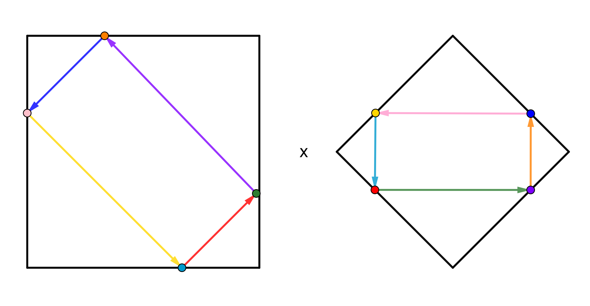
Figure 1. Systoles that don’t contain diagonals of $B_{\infty}$ or $B_{1}$.

This picture illustrates the dynamics of systoles. Since systoles must lie in the boundary of $B_{\infty}\times B_{1}$, it follows that either $(x_{1},x_{2})$ must lie on the boundary of $B_{\infty}$ or $(y_{1},y_{2})$ must lie on the boundary of $B_{1}$. We can assume that $(x_{1},x_{2})$ belongs to the boundary of $B_{\infty}$ and is not one of the corners of $B_{\infty}$.

For example, let $(x_{1},x_{2})$ be the green node in Figure 1. Then, whichever coordinate $(y_{1},y_{2})$ in $B_{1}$ we choose, it must move in the direction of the green vector until it hits the boundary of $B_{1}$ (the purple node in the picture). At this point, the systole cannot move in the direction of the green arrow anymore, since it has to stay inside $\partial(B_{\infty}\times B_{1})$. Therefore, $(y_{1},y_{2})$ must stay constant. If we chose $(y_{1},y_{2})$ to be off the diagonals, there is only one direction in which $(x_{1},x_{2})$ can now move. That is in the direction of the purple vector until it hits the boundary of $B_{\infty}$ (the orange node in Figure 1). This alternating process then continues in the same manner.

By narrowing rectangles in $B_{1}$ in the vertical direction, we obtain, in the uniform limit, systoles illustrated in Figure 2.

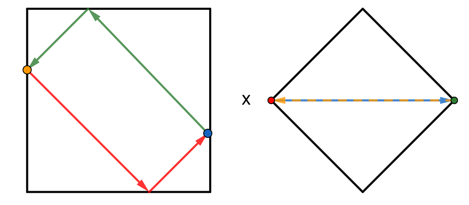
Figure 2. Systoles whose projection onto $B_{1}$ is the horizontal diagonal of $B_{1}$.

The dynamics of these systoles differ in the following way. Consider, for example, the red node on $\partial B_{1}$. If $(x_{1},x_{2})\in B_{\infty}$, the subdifferential of $H_{B_{\infty}\times B_{1}}$ at the point $(x_{1},x_{2},-1,0)$ contains the convex hull of the vectors $(0,0,-2,-2)$ and $(0,0,-2,2)$. As a result, the red arrow in $B_{\infty}$ can change direction at any point, taking a direction such that the angle measured from the horizontal axis lies within the range $[-\frac{\pi}{4},\frac{\pi}{4}]$. Notice that the directions of the red arrows in the picture correspond to the extremal directions.

Using an analogous process, we can obtain systoles that involve other diagonals in $B_{\infty}$ and $B_{1}$.

By shrinking both rectangles, we get systoles that are completely contained within the diagonals of $B_{\infty}$ and $B_{1}$. One such systole is illustrated in Figure 3.

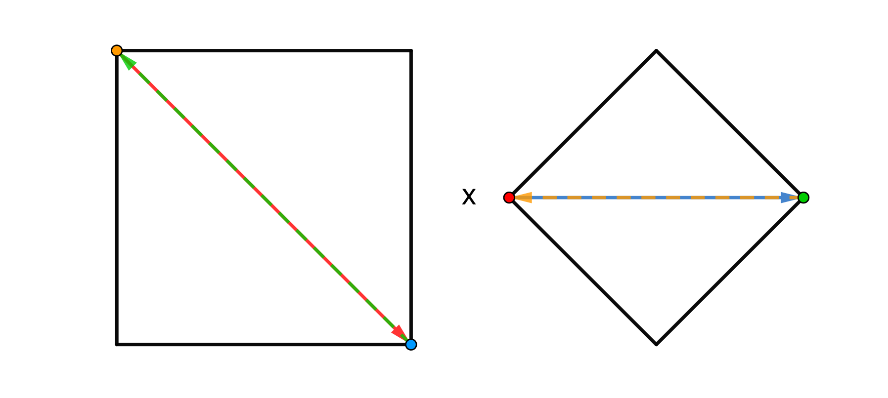
Figure 3. Diagonal systole on $\partial(B_{\infty}\times B_{1})$.

The $S^{1}$-invariant subset of systoles $\widetilde{\operatorname{Sys}}(\partial(B_{\infty}\times B_{1}))\subseteq\operatorname{Sys}(\partial(B_{\infty}\times B_{1}))$, consisting of the previously described systoles, is such that the $\text{ev}_{0}$ is a bijection on this space. Moreover, it is evident that $\widetilde{\operatorname{Sys}}(\partial(B_{\infty}\times B_{1}))$ is closed since it is defined as the uniform closure of the space of systoles illustrated in Figure 1. This implies, by the previous proposition, that $B_{\infty}\times B_{1}$ is generalized Zoll. In particular, $\text{ev}_{0}(\partial(B_{\infty}\times B_{1}))=\partial(B_{\infty}\times B_{1})$.

References

• [Abb99] Alberto Abbondandolo. Morse theory for strongly indefinite functionals and Hamiltonian systems. PhD thesis, Scuola Normale Superiore, 1999.
• [Abb01] A. Abbondandolo, Morse theory for Hamiltonian systems, Pitman Research Notes in Mathematics, vol. 425, Chapman & Hall, London, 2001.
• [AB23] Abbondandolo, A., Benedetti, G. On the local systolic optimality of Zoll contact forms. Geom. Funct. Anal. 33, 299–363 (2023). https://doi.org/10.1007/s00039-023-00624-z
• [ABE23] A. Abbondandolo, G. Benedetti, O. Edtmair, Symplectic capacities of domains close to the ball and Banach-Mazur geodesics in the space of contact forms, arXiv:2312.07363 [math.SG], 2023.
• [AK22] A. Abbondandolo, J. Kang, Symplectic homology of convex domains and Clarke’s duality, Duke Mathematical Journal, Duke Math. J. 171(3), 739-830, 2022.
• [AO08] Shiri Artstein-Avidan, Yaron Ostrover, A Brunn–Minkowski Inequality for Symplectic Capacities of Convex Domains, International Mathematics Research Notices, Volume 2008, 2008, rnn044.
• [AO14] Shiri Artstein-Avidan, Yaron Ostrover, Bounds for Minkowski Billiard Trajectories in Convex Bodies, International Mathematics Research Notices, Volume 2014, Issue 1, 2014, Pages 165–193.
• [BBLM23] L. Baracco, O. Bernardi, C. Lange, M. Mazzucchelli, On the local maximizers of higher capacity ratios, (2023), arXiv:2303.13348.
• [Ben82] V. Benci, On critical point theory for indefinite functionals in the presence of symmetries, Trans. Amer. Math. Soc. 274 (1982), no. 2, 533–572.
• [Cla79] F. H. Clarke, A classical variational principle for periodic Hamiltonian trajectories, Proc. Amer. Math. Soc. 76 (1979), 186–188.
• [Cla81] F. H. Clarke, Periodic solutions to Hamiltonian inclusions, J. Differential Equations 40 (1981), 1–6.
• [Cla83] F.H. Clarke, Optimization and Nonsmooth Analysis, John Wiley and Sons, New York (1983).
• [EH87] I. Ekeland and H. Hofer, Convex Hamiltonian energy surfaces and their periodic trajectories, Comm. Math. Phys. 113 (1987), no. 3, 419–469. MR925924.
• [EH89] I. Ekeland and H. Hofer, Symplectic topology and Hamiltonian dynamics, Math. Z. 200 (1989), no. 3, 355–378. MR978597.
• [EH90] I. Ekeland and H. Hofer, Symplectic topology and Hamiltonian dynamics. II, Math. Z. 203 (1990), no. 4, 553–567. MR1044064.
• [FR78] Edward R. Fadell and Paul H. Rabinowitz, Generalized cohomological index theories for Lie group actions with an application to bifurcation questions for Hamiltonian systems, Invent. Math. 45 (1978), no. 2, 139–174. MR478189.
• [GH18] J. Gutt, M. Hutchings, Symplectic capacities from positive $S^{1}$–equivariant symplectic homology, Algebraic $\&$ Geometric Topology, Algebr. Geom. Topol. 18(6), 3537-3600, (2018).
• [GGM21] V. L. Ginzburg, B. Z. Gurel, M. Mazzucchelli, On the spectral characterization of Besse and Zoll Reeb flows, Ann. Inst. H. Poincare C Anal. Non Lineaire 38 (2021), no. 3, 549–576. MR4227045.
• [GHR22] J. Gutt , M. Hutchings, V.G.B. Ramos, Examples around the strong Viterbo conjecture. J. Fixed Point Theory Appl. 24, 41 (2022). https://doi.org/10.1007/s11784-022-00949-6
• [GR24] J. Gutt, V. G. B. Ramos, The equivalence of Ekeland-Hofer and equivariant symplectic homology capacities, arXiv:2412.09555.
• [HZ94] H. Hofer, E. Zehnder, E. Symplectic Invariants and Hamiltonian Dynamics, BirkhΓ€user, Basel (1994).
• [Joh48] F. John. Extremum problems with inequalities as subsidiary conditions. Courant Anniversary volume, Interscience New-York 1948.
• [LMS13] J. Latschev, D. McDuff, F. Schlenk, The Gromov width of 4-dimensional tori, Geom. Topol. 17 (2013) 2813-2853.
• [Mat24] S. MatijeviΔ‡, Positive ($S^{1}$-equivariant) symplectic homology of convex domains, higher capacities, and Clarke’s duality, arXiv:2410.13673.
• [MR23] M. Mazzucchelli and M. Radeschi, On the structure of Besse convex contact spheres, Trans. Amer. Math. Soc. 376 (2023), no. 3, 2125–2153. MR4549701.
• [Rud22] D. Rudolf, Viterbo’s conjecture for Lagrangian products in $\mathbb{R}^{4}$ and symplectomorphisms to the Euclidean ball, arXiv:2203.02294.
• [Sch05] F. Schlenk, Embedding Problems in Symplectic Geometry, De Gruyter Expositions in Mathematics 40, Walter de Gruyter Verlag, Berlin, 2005.
• [Tra95] L. Traynor, Symplectic packing constructions, J. Differential Geometry 41 (1995) 735-751.
• [Vit00] C. Viterbo, Metric and isoperimetric problems in symplectic geometry, J. Amer. Math. Soc. 13 (2000), no. 2, 411–431.
• [Whi35] H. Whitney, A function not constant on a connected set of critical points, Duke Mathematical Journal, Duke Math. J. 1(4), 514-517, 1935.