Cutting a unit square and permuting blocks

Abstract.

Consider a random permutation of $kn$ objects that permutes $n$ disjoint blocks of size $k$ and then permutes elements within each block. Normalizing its cycle lengths by $kn$ gives a random partition of unity, and we derive the limit law of this partition as $k,n\to\infty$. The limit may be constructed via a simple square cutting procedure that generalizes stick breaking in the classical case of uniform permutations ($k=1$). The proof is by coupling, providing upper and lower bounds on the Wasserstein distance. The limit is shown to have a certain self-similar structure that gives the distribution of large cycles and relates to a multiplicative function involving the Dickman function. Along the way we also give the first extension of the Erdős-Turán law to a proper permutation subgroup.

1. Introduction

This paper concerns the cycles of large random permutations with a certain block structure imposed. This structure results in rich phenomena in the limit that can be seen as different instances of self-similar behavior. We provide a simple combinatorial description that underlies such behavior and generalizes old results in the “anatomy of integers and permutations" [granville2008anatomy].

Permutations acting on blocks as described in the abstract are known to algebraists as wreath products, which are a certain semidirect product. Elements $\sigma$ of the wreath product subgroup $S_{k}^{n}\rtimes S_{n}\leq S_{kn}$ will be represented as

$$\sigma=(g_{1},\ldots,g_{n};h),\qquad g_{i}\in S_{k},\ h\in S_{n}$$

This permutes $\{1,\dots,kn\}$ with $g_{1}$ permuting $\{1,\dots,k\}$, $g_{2}$ permuting $\{k+1,\dots,2k\}$, $\ldots$, $g_{n}$ permuting $\{(n-1)k+1,\dots,kn\}$ independently and then $h$ permuting the $n$ blocks. Such permutations are the focus of [diaconis2024poisson]. For example $\sigma=((12),(1)(2),(12);(312))\in S_{2}^{3}\rtimes S_{3}$ permutes 1 2 3 4 5 6 first to 2 1 3 4 6 5 and then 6 5 2 1 3 4. In the usual two-line notation for permutations,

1	2	3	4	5	6
6	5	2	1	3	4

has cycle decomposition $(164)(253)$.

1.1. Partitions of unity and cycles of random permutations

First we motivate and state the main result, Theorem 1.1. Our story starts with the stick breaking interpretation of the Poisson-Dirichlet distribution on partitions of unity (nonnegative numbers summing to 1, defined more carefully in Section 5). This distribution has seen many beautiful constructions from fundamental discrete objects, such as cycles of permutations and prime factors of integers. Some of these are surveyed in [tao], where emphasis is placed on the commonalities between these seemingly disparate instances; we attempt to do the same with our square cutting distribution. The Poisson-Dirichlet has seen generalization [pitman1997two] and continues to appear in recent work on spatial random permutations such as the interchange process [elboim2022infinite]. It is also the equilibrium measure for certain coagulation and fragmentation processes [pitman2006combinatorial]. To construct the Poisson-Dirichlet, consider the following process: break a stick of length 1 uniformly, set the right piece aside, and repeat the process on the left piece. The randomness for break points can be sampled as $U_{1},U_{2},\dots$ iid $U[0,1]$ and the stick lengths are then

$$\Sigma=\left\{U_{1},(1-U_{1})U_{2},(1-U_{1})(1-U_{2})U_{3},\dots\right\}$$ (1)

We will think of this random partition as being characterized by a self-similarity property

$$\Sigma=\left\{U,(1-U)\Sigma\right\}$$ (2)

in distribution, where $U\sim U[0,1]$ independent of $\Sigma$. It is a standard result that the partition of unity given by normalizing the cycle type of a random permutation in $S_{n}$ converges to $\Sigma$ as $n\to\infty$ [schmidt1977limit]. A nice heuristic argument is given in [tao], for example. Here we extend this stick-breaking interpretation to wreath product permutations, which gives a sort of two dimensional analog.

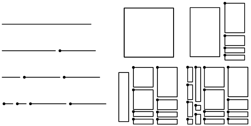
Figure 1. Stick breaking construction of the Poisson-Dirichlet and square cutting construction of $\mathcal{P}$. Each step of square cutting consists of vertically cutting the leftmost rectangle as well as horizontally cutting the new piece.

1.1.1. Square Cutting

The following is a generalization of the stick breaking procedure that turns out to describe the limit of $\left\{\frac{C_{1}}{kn},\frac{C_{2}}{kn},\dots\right\}$ where $C_{1},C_{2},\dots$ are the cycle lengths of $\sigma\in S_{k}^{n}\rtimes S_{n}$, as both $k,n\to\infty$. Take a unit square, slice off a rectangle vertically at a uniform point on the top edge, set aside the right rectangle, and repeat on the left. After this is done, take all the pieces and repeat the process slicing horizontally. That is slice horizontally at a uniform point on the left edge, set aside the top piece, and repeat on the bottom (see Figure 1). The final areas of all rectangles are a random partition of unity from the limit law of $\left\{\frac{C_{1}}{kn},\frac{C_{2}}{kn},\dots\right\}$.

As with stick breaking, the randomness can be sampled by $\left\{U_{i,j}\right\}_{i,j=1}^{\infty}$ iid $U[0,1]$ random variables. Encoding the above description the areas of the final pieces are

$$\mathcal{P}=\{ U_{1,1}U_{1,2};U_{1,1}(1-U_{1,2})U_{1,3};U_{1,1}(1-U_{1,2})(1-U_{1,3})U_{1,4};\dots$$ (3)

$$(1-U_{1,1})U_{2,1}U_{2,2};(1-U_{1,1})U_{2,1}(1-U_{2,2})U_{2,3};(1-U_{1,1})U_{2,1}(1-U_{2,2})(1-U_{2,3})U_{2,4};\dots$$

$$(1-U_{1,1})(1-U_{2,1})U_{3,1}U_{3,2};\dots\}$$

which exhibits the self-similar structure

$$\mathcal{P}=\left\{U\Sigma,(1-U)\mathcal{P}\right\}$$ (4)

where $U\sim U[0,1]$ and $\Sigma$ is Poisson-Dirichlet distributed, both independent of $\mathcal{P}$.

1.1.2. Main Result

Our main result is then the convergence of the partition given by cycles of a wreath product permutation to this partition. Let $\Delta\subset[0,1]^{\mathbb{N}}$ be the space of partitions and $\rho$ a metric on $\Delta$. If $X,Y$ are two random partitions with laws $\mu,\nu$ respectively let

$$d_{\rho}(X,Y)\coloneqq\sup\left\{\int_{\Delta}f(x)d(\mu-\nu)(x):f\text{ continuous and Lip}_{\rho}(f)\leq 1\right\}=\inf\mathbb{E}_{(X,Y)}\rho(x,y)$$

be the Wasserstein or transport metric, where the infimum is over all couplings $(X,Y)$. Our main result gives weak convergence of wreath product cycle partitions to the square cutting distribution, with rates.

Theorem 1.1 (Square cutting).

Let $\Sigma,\mathcal{P}$ be partitions of unity defined by

$$\Sigma=(U,(1-U)\Sigma),\quad\mathcal{P}=(\tilde{U}\Sigma,(1-\tilde{U})\mathcal{P})$$

in distribution where $U,\tilde{U}$ are independent and uniformly distributed in the unit interval. Take $\pi\in S_{k}^{n}\rtimes S_{n}$ uniformly and let $C_{1},C_{2}\dots$ be the cycle lengths in $\pi$. Let $C=\left(\frac{C_{1}}{kn},\frac{C_{2}}{kn},\dots\right)$. Then

$$d_{L^{\infty}}(C,\mathcal{P})\leq 1/k+1/n$$

and

$$\frac{\log^{2}(kn)}{8kn}\leq d_{L^{1}}(C,\mathcal{P})\leq\frac{3(\log k+\gamma)}{k}+\frac{3(\log n+\gamma)}{n}+O(1/k^{2}+1/n^{2})$$

where $\gamma$ is the Euler-Mascheroni constant and the implied constant is universal.

Note that this is a natural choice of distance since an upper bound of $o_{k,n}(1)$ implies weak convergence. There is no hope, however, of bounding total variation distance as $C$ is supported on rationals almost surely for any $k,n$ but $\mathcal{P}$ consists almost surely of irrational lengths. The proof in Section 5 actually shows that the $L^{\infty}$ bound is uniform and not random at all. That is, under the coupling

$$\lVert C-\mathcal{P}\rVert_{\infty}\leq 1/k+1/n$$

always. This can be used to bound $d_{L^{p}}(C,\mathcal{P})$ for any $p>1$ by pulling out the largest term repeatedly until one reaches $d_{L^{1}}(C,\mathcal{P})$.

Using the same coupling we also give a convergence result for the non-normalized cycle counts in Appendix A to compound Poisson limits. Without normalization the cycle lengths constitute integer partitions, well-studied objects that in fact gave rise to the Hardy-Littlewood circle method [hardy1918asymptotic]. Compound Poisson limits show up in other places and can be established with an extension of Stein’s method [barbour1992compound], although ours comes from elementary Poisson splitting.

1.2. Structure of the paper

Section 2 extends the Erdős-Turán law for the least common multiple of cycle lengths to wreath product subgroups. Sections 3 and 4 then explore the self-similarity properties of the largest part of $\mathcal{P}$, where connections with the Dickman function and multiplicative number theory arise. With cycle statistics being a strong motivator for studying random partitions like $\pi$ we then extend results to general wreath products of the form $\Gamma^{n}\rtimes S_{n}$ which correspond to choosing the permutation of each block uniformly from $\Gamma\subseteq S_{k}$. These include an extension of the main convergence result to more general random partitions in Section 5 and analysis of the $k$-th largest part for $k\geq 1$ in Section 6. This fills a gap left open by [diaconis2024poisson], where limits of cycle counts and various patterns are derived but their methods are unable to address large cycles. Finally, Section 7 remarks on closed form expressions for the distribution functions given in Section 6 and gives an asymptotic bound in a special case of interest.

1.3. Acknowledgements

The author thanks Persi Diaconis for encouraging the pursuit of quantitative results and helpful discussions, as well as Kannan Soundararajan for pointing out the connection to multiplicative functions.

2. Erdős-Turán law for wreath products

As a warmup we investigate the product structure of cycles in wreath permutations and use it to extend a result of Erdős and Turán giving a lognormal distribution for the least common multiple of cycle lengths [erdHos1967some]. Their result has seen generalization to the Ewens sampling distribution [arratia1992limit] but this is the first extension to a uniform permutation from a proper nontrivial subgroup.

Considering $\sigma=(g_{1},\dots,g_{n};h)\in S_{k}^{n}\rtimes S_{n}$ its cycle lengths are given by products of cycle lengths involving the $g_{i}$ and $h$. Consider an $m$-cycle $(1h(1)h^{2}(1)\dots h^{m}(1))$ in $h$, where $h^{i}$ is $h$ composed with itself $i$ times. Then taking $g_{1}\circ g_{h(1)}\circ g_{h^{2}(1)}\circ\dots\circ g_{h^{m}(1)}\in S_{k}$ we may decompose it into cycles of length $G_{1},\dots,G_{l}$ and these combine with the $m$-cycle in $h$ to make cycles of lengths $mG_{1},\dots,mG_{l}$ in $\sigma$. This happens for all cycles in $h$ and corresponding compositions of $g$’s. In the example from Section 1 the only cycle in $h$ is the $3$-cycle $(312)$. Then $g_{3}\circ g_{1}\circ g_{2}=(12)\circ(12)\circ(1)(2)=(1)(2)$ decomposes into two fixed points and the final cycle lengths, two $3$-cycles, are both given as $3*1$. Applying this to a simple coupling gives the following.

Theorem 2.1 (Wreath product Erdős-Turán).

Let $\Gamma\subseteq S_{k}$ be arbitrary and $C_{1},C_{2},\dots$ the cycle lengths in a uniform permutation from $\Gamma^{n}\rtimes S_{n}$. Let $O_{n}=\operatorname*{lcm}\left\{C_{1},C_{2},\dots\right\}$. Then

$$\frac{\log O_{n}-\frac{1}{2}\log^{2}n}{\sqrt{\frac{1}{3}\log^{3}n}}\stackrel{{\scriptstyle d}}{{\longrightarrow}}N(0,1)$$

as $n\to\infty$ for fixed $k$. If $\Gamma=C_{k}$, the result holds for $k=e^{o(\log^{3/2}n)}$.

Proof.

Let the permutation in the theorem be $\sigma=(g_{1},\dots,g_{n};h)$ and $P_{n}$ be the least common multiple of cycle lengths of a uniform $\pi\in S_{n}$. The original result of Erdős and Turán then gives the exact same limit law with $P_{n}$ in place of $O_{n}$. We can then couple $O_{n}$ and $P_{n}$ by setting $h=\pi$ so that

$$\log P_{n}\leq\log O_{n}\leq\log P_{n}+O_{k}(1)$$

which gives the result. This is because each permutation in $S_{k}$ of the form $g_{1}\circ g_{h(1)}\circ\dots$ decomposes into cycles of length $G_{1},G_{2}\dots\leq k$. When multiplied by lengths in $h=\pi$ these increase the least common multiple by a factor of at most $\operatorname*{lcm}([k])\leq k!=O_{k}(1)$. If $\Gamma=C_{k}$ then

$$\log P_{n}\leq\log O_{n}\leq\log P_{n}+\log k$$

since $G_{1},G_{2},\dots$ all divide $k$. Then if $\log k=o(\log^{3/2}n)$ the error term converges to $0$ when normalized.

∎

It would be interesting to see which subgroups $\Gamma\leq S_{k}$ allow one to take $k$ large with $n$ in the above theorem, and how large. For instance with $\Gamma=S_{k}$ one has

$$O_{n}=\operatorname*{lcm}(C_{1}*\operatorname*{lcm}(\pi_{1}),C_{2}*\operatorname*{lcm}(\pi_{2}),\dots)$$

where $\pi_{1},\pi_{2},\dots$ are iid uniform from $S_{k}$ and $C_{1},C_{2},\dots$ are the cycle lengths in a uniform permutation from $S_{n}$. It’s not clear how large $k$ can be taken in this case.

3. Largest part

This section derives the distribution of the largest part of $\mathcal{P}$ as defined in Theorem 1. First recall the Dickman function [tenenbaum2015introduction], denoted $\rho$, which may be defined as the unique function satisfying the delay differential equation

$$u\rho^{\prime}(u)+\rho(u-1)=0$$

for $u\geq 0$ with initial conditions $\rho(u)=1$ for $u\in[0,1]$ (more on this in Section 4).

Theorem 3.1 (Largest piece from square cutting).

Let $\mathcal{N}$ be the area of the largest piece in $\mathcal{P}$. Then $\mathcal{N}$ has distribution function $F(u)=\pi(1/u)$ where $\pi$ is defined by

$$\pi(u)=\frac{1}{u}(\pi\ast\rho)(u)$$

for $u>0$ with $\pi(u)=1$ for $u\in[0,1]$.

Proof.

Let $\mathcal{M}$ be the largest element of $\Sigma$ (length of the longest stick). Then

$$\phi(x) \coloneqq F(1/x)=\mathbb{P}\left(\mathcal{N}\leq 1/x\right)=\mathbb{P}\left(\max(U\mathcal{M},(1-U)\mathcal{N})\leq 1/x\right)$$

$$=\int_{0}^{1}\mathbb{P}\left(\max(t\mathcal{M},(1-t)\mathcal{N})\leq 1/x\right)dt$$

$$=\int_{0}^{1}\mathbb{P}\left(\mathcal{M}\leq\frac{1}{xt}\right)\mathbb{P}\left(\mathcal{N}\leq\frac{1}{x(1-t)}\right)dt$$

$$=\int_{0}^{1}\rho(xt)\phi(x(1-t))dt$$

$$=\frac{1}{x}\int_{0}^{x}\rho(y)\phi(x-y)dy$$

which is exactly the defining property of $\pi$, so $\phi=\pi$. The penultimate equality is the classical result that the distribution of the largest piece of a Poisson-Dirichlet distributed partition is given by Dickman’s function, but can also be seen by running this exact proof with $\mathcal{N}=\mathcal{M}$ and using (2) instead of (4). Indeed

$$\rho(u)=\frac{1}{u}\int_{u-1}^{u}\rho(t)dt=\frac{1}{u}\int_{0}^{u}\rho(t)1_{[0,1]}(u-t)dt=\frac{1}{u}(\rho\ast 1_{[0,1]})(u)$$

and the rest goes through as is. ∎

The proof illustrates how self-similarity properties like (2) and (4) naturally lead to a convolutional structure on the distribution of large parts of partitions. It is then of interest to study general distribution functions of this convolutional form.

4. Integral equations and a multiplicative function

For any function $\psi:[0,\infty)\to[0,1]$ with $\psi(x)=1$ for $x\in[0,1]$, consider the function $\phi$ defined by

$$\phi(x)=\frac{1}{x}(\phi\ast\psi)(x)=\frac{1}{x}\int_{0}^{x}\phi(t)\psi(x-t)dt$$ (5)

with $\phi(x)=1$ for $x\in[0,1]$. Such equations arise in the study of the spectrum of multiplicative functions in [granville2001spectrum], where basic existence and uniqueness properties are established. These also show up as the stationary distributions of iterated random functions as in [diaconis1999iterated]. Dickman’s function $\rho$ and $\pi$ above are examples, and $\pi$ can be thought of as one step above $\rho$ in a self-similarity hierarchy: $\pi$ is defined via convolution with $\rho$ which is in turn defined via convolution with $1_{[0,1]}$.

In light of this and that the Dickman function from number theory arises in the largest cycle of a permutation, one may hope to make a number theoretic statement involving $\pi$ which has shown up in the largest cycle of a wreath product permutation. Recall that $\rho$ is also characterized by

$$\rho(u)=\lim_{x\to\infty}\frac{\left\lvert\left\{n\leq x:p(n)\leq x^{1/u}\right\}\right\rvert}{x}$$

where $p(n)$ denotes the largest prime factor of the integer $n$. Put another way, $\rho(u)$ is the limit of probabilities that a uniformly sampled integer from $[x]$ has all prime factors at most $x^{1/u}$ [tao, moree2014integers]. While it would be nice to have such a probabilistic description of $\pi$, it seems the most immediate generalization of this idea lies in thinking of $\rho$ as a multiplicative function. Defining $f_{x}(p)=1_{p\leq x}$ and $f_{x}(nm)=f_{x}(n)f_{x}(m)$ for coprime $n,m$ we have

$$\rho(u)=\lim_{x\to\infty}\frac{1}{x^{u}}\sum_{n\leq x^{u}}f_{x}(n)$$

Here is the analog for $\pi$

Theorem 4.1 (Mean of a multiplicative function).

With $f_{x}(p)=\rho\left(\frac{\log p}{\log x}\right)$ totally multiplicative and $\pi$ as in Theorem 3.1, for $u>0$

$$\pi(u)=\lim_{x\to\infty}\frac{1}{x^{u}}\sum_{n\leq x^{u}}f_{x}(n)$$

First we establish a way to approximate a sum over primes by an integral

Lemma 4.2 (Integral approximation).

For large $x$ and $c$ any function, let $g_{c(x)}(y),y\geq 0$ be a family of differentiable functions with $\lim_{y\to\infty}g_{c(x)}(y)=0$ and suppose $g_{c(x)}(x)=o\left(e^{-\varepsilon\sqrt{\log x}}\right)$ for every fixed positive $\varepsilon$. Then

$$\sum_{p\leq x}g_{c(x)}(p)=\int_{2}^{x}\frac{g_{c(x)}(t)}{\log t}dt+o(x)$$

Proof.

Using summation by parts and the de la Vallée Poussin approximation to the prime counting function $\pi(x)=\left\lvert\left\{p:p\leq x\right\}\right\rvert$ [ingham1990distribution]

$$\sum_{p\leq x}g_{c(x)}(p) =-\sum_{p\leq x}\int_{2}^{\infty}g^{\prime}_{c(x)}(t)1_{t\geq p}dt=-\int_{2}^{\infty}g^{\prime}_{c(x)}(t)\pi(x\wedge t)dt$$

$$=\pi(x)g_{c(x)}(x)-\int_{2}^{x}g^{\prime}_{c(x)}(t)\pi(t)dt$$

$$=g_{c(x)}(x)\int_{2}^{x}\frac{1}{\log t}dt+O\left(g_{c(x)}(x)xe^{-a\sqrt{\log x}}\right)$$

$$-\int_{2}^{x}g^{\prime}_{c(x)}(t)\int_{2}^{t}\frac{1}{\log s}dsdt+O\left(\int_{2}^{x}g^{\prime}_{c(x)}(t)te^{-a\sqrt{\log t}}dt\right)$$

for some positive $a$. Now integrating by parts both terms in the last line, cancelling, and combining error terms one has the result. ∎

Proof of Theorem 4.1.

Let $\mathcal{V}(x)=\sum_{p\leq x}\log p$. By Proposition 1 of [granville2001spectrum] it suffices to verify that

$$\rho(u)=\lim_{x\to\infty}\frac{1}{\mathcal{V}(x^{u})}\sum_{p\leq x^{u}}\rho\left(\frac{\log p}{\log x}\right)\log p$$

as then by bounded convergence one may pass the limit inside the convolution. Since $g_{x}(y)=\log(y)$ satisfies the assumptions, applying Lemma 4.2

$$\mathcal{V}(x^{u})=x^{u}+o(x^{u})$$

Now $g_{x}(y)=\rho\left(\frac{\log y}{\log x}\right)\log y$ is differentiable since the Dickman function is, and also $g_{x}(x^{u})=u\rho(u)\log x=o\left(e^{-\varepsilon\sqrt{u\log x}}\right)$ for every positive $\varepsilon$. Applying the lemma again

$$\sum_{p\leq x^{u}}\rho\left(\frac{\log p}{\log x}\right)\log p =\int_{2}^{x^{u}}\rho\left(\frac{\log t}{\log x}\right)dt+o(x^{u})$$

so we are left with

$$\lim_{x\to\infty}\frac{\int_{2}^{x^{u}}\rho\left(\frac{\log t}{\log x}\right)dt+o(x^{u})}{x^{u}+o(x^{u})}=\lim_{x\to\infty}\frac{1}{x^{u}}\int_{2}^{x^{u}}\rho\left(\frac{\log t}{\log x}\right)dt$$

$$=\lim_{x\to\infty}\frac{1}{ux^{u-1}}\left(ux^{u-1}\rho(u)-\int_{2}^{x^{u}}\rho^{\prime}\left(\frac{\log t}{\log x}\right)\frac{\log t}{x\log^{2}x}dt\right)$$

$$=\rho(u)$$

as desired. ∎

It may be interesting to study distributions with density proportional to the solution of an integral equation (as opposed to distribution function as we have seen so far). This has been done in the case of the Dickman function and there are many elegant and fundamental constructions of such a distribution, some even relating to cycles of permutations, as well as established properties like infinite divisibility [molchanov2020dickman]. Essentially from definition, distributions with density proportional to the solution of an integral equation have characteristic (random) operators that allow for Stein’s method. If $X$ has density $\phi$ and $Y$ has density $\psi$ related as in (5) then

$$\mathbb{E}[Xf(X)]=\int_{0}^{\infty}tf(t)\phi(t)dt=\int_{0}^{\infty}f(t)(\phi\ast\psi)(t)dt=\mathbb{E}[f(X+Y)]$$

Applying this to the laplace transform $L_{X}(s)=\mathbb{E}e^{-sX}$ gives the self-similarity property

$$L^{\prime}_{X}(s)=-L_{Y}(s)L_{X}(s)$$

which can be used to derive the transform of random variables with Dickman or $\pi$ density. This is essentially the fact that the Fourier transform takes convolution to multiplication.

5. Proof of theorem 1.1 and extension

5.1. Coupling

This section provides the key coupling methods used in the proofs of Theorems 1.1 and A.1. We start with briefly recalling the Feller coupling, which gives a way to directly sample the cycle type of a permutation using a binary sequence without dealing at all with the permutation itself.

Let $\xi_{1},\xi_{2},\dots$ be independent such that $\mathbb{P}\left(\xi_{i}=1\right)=1/i$ and $\xi_{i}=0$ otherwise. We call the pattern $\xi_{i}\xi_{i+1}\dots\xi_{i+k}=10^{k-1}1$ a $k$-space starting at $i$. Let $A=(A_{1},A_{2},\dots)$ and $Z=(Z_{1},Z_{2},\dots)$ be such that $A_{k}$ denotes the number of $k$-spaces in $\Xi_{n}\coloneqq 1\xi_{2}\xi_{3}\dots\xi_{n}1$ and $Z_{k}$ denotes the number of $k$-spaces in $\Xi\coloneqq 1\xi_{2}\xi_{3}\dots$. Then the Feller coupling asserts that the number of $k$-cycles in a uniform permutation from $S_{n}$ is distributed as $A_{k}$ [najnudel2020feller, diaconis2024poisson], $A_{k}\to Z_{k}$ as $n\to\infty$, and that $Z_{k}\sim\operatorname{Poi}(1/k)$ independently [ignatov1982constant].

We will also use a normalized version of the Feller coupling, that allows one to obtain the normalized cycle lengths from a Poisson process on $[0,1]$. Looking at the binary sequence on the unit interval, with $\xi_{i}$ marking $(i-1)/n$, the occurence of $1$’s may be thought of as a process where the lengths of time between arrivals gives a partition of unity arising from the permutation. We couple this process to the poisson process $X$ on the interval $t\in[0,1]$ with rate $1/t$.

Let $x_{1}\geq x_{2}\geq\dots\in[0,1]$ be the arrival times of $X$ and $X[a,b]=\left\lvert\left\{x_{i}\in[a,b]\right\}\right\rvert$. Note that

$$\mathbb{P}\left(X\left[\frac{j-1}{n},\frac{j}{n}\right]=0\right)=\exp\left(-\int_{\frac{j-1}{n}}^{\frac{j}{n}}\frac{1}{t}dt\right)=1-\frac{1}{j}$$

which is exactly $\mathbb{P}\left(\xi_{j}\right)=0$. It’s known [ignatov1982constant] that the partition $\Sigma=(1-x_{1},x_{1}-x_{2},x_{2}-x_{3},\dots)$ is Poisson-Dirichlet distributed, and indeed the above computation can show that $1-x_{1}$ is uniformly distributed in the interval, linking this to the stick breaking interpretation in Section 1; this coupling can equivalently be carried out by coupling uniform with discrete uniform. To couple round $y_{i}=\frac{\left\lfloor nx_{i}\right\rfloor}{n}$ and let $\Sigma_{n}=(1-y_{1},y_{1}-y_{2},\dots)$ with at most $n$ nonzero entries. From the above computation $\Sigma_{n}$ is a random partition from the binary process and thus the random partition arising from the normalized cycle lengths of a uniform $\sigma\in S_{n}$.

5.2. Proof of Theorem 1.1

This section first proves Theorem 1.1 and then generalizes to $\Gamma^{n}\rtimes S_{n}$ for arbitrary $\Gamma\leq S_{k}$ with only $n\to\infty$. A similar generalization is easily achieved in the same way for $S_{k}^{n}\rtimes\Gamma$ for $\Gamma\leq S_{n}$ and $k\to\infty$ but we do not write out the details here. It should be noted that if one desires only a weak convergence statement of Theorem 1.1 without rates then coupling is not needed; the analagous statement for uniform random permutations from $S_{k}$ and $S_{n}$ can be bootstrapped to give convergence for $S_{k}^{n}\rtimes S_{n}$.

We must formalize the space of partitions of unity introduced in Section 1.1. One generally hopes to define partitions to be invariant under permutation, but doing so makes them hard to compare and operate with. We follow the lead of past literature and sort them in nonincreasing order, stating results for ordered partitions as vectors. Define the infinite simplex and its subset of nonincreasing vectors

$$\bar{\Delta} \coloneqq\left\{x=(x_{1},x_{2},\dots):x_{i}\geq 0,\text{ and }\sum_{i=1}^{\infty}x_{i}=1\right\},\quad\Delta\coloneqq\left\{x\in\bar{\Delta}:x_{1}\geq x_{2}\geq\dots\right\}$$

There is then a natural projection from $\bar{\Delta}\to\Delta$ that simply sorts a vector. We will think of a partition of unity as being both the preimage of an $x\in\Delta$ (like a multiset) as well as $x$ itself, depending on what’s more convenient. Thus if it’s asserted that $x=y$ for two partitions that are not necessarily nonincreasing, what’s really meant is that their projections to $\Delta$ are equal.

Some key features of the coupling $(\Sigma_{n},\Sigma)$ in section 5.1 are

$$\lVert\Sigma-\Sigma_{n}\rVert_{\infty}\leq 1/n,\quad\mathbb{E}\lVert\Sigma-\Sigma_{n}\rVert_{1}\leq\frac{3(\log n+\gamma)}{n}+O(1/n^{2})$$

The first is immediate, so consider the second. Each nonzero part $y_{i}-y_{i+1}$ of $\Sigma_{n}$ can be identified with a part $x_{j}-x_{j+1}$ of $\Sigma$ by choosing $j=\min\left\{k:x_{k}\in(y_{i},y_{i}+\frac{1}{n}]\right\}$. Then these parts differ in length by at most $2/n$, and the total length of parts $\left\{x_{k}-x_{k+1}:x_{k}\in(y_{i},y_{i}+\frac{1}{n}],k\neq j\right\}$ is at most $1/n$. Doing this for all nonzero parts of $\Sigma_{n}$ gives the bound $\lVert\Sigma_{n}-\Sigma\rVert_{1}\leq\frac{3}{n}\left\lvert\Sigma_{n}\right\rvert$. Then using that the expected number of cycles in a uniform permutation from $S_{n}$ is the harmonic number $H_{n}$ we have

$$\mathbb{E}\lVert\Sigma_{n}-\Sigma\rVert_{1}\leq\frac{3}{n}H_{n}\leq\frac{3(\log n+\gamma)}{n}+O(1/n^{2})$$

In order to extend this coupling to wreath products we need any pairing function $\mathbb{N}^{2}\to\mathbb{N}$ to collapse a sequence of partitions into a single partition. To make an explicit choice take $g(i,j)=2^{i-1}(2^{j}-1)$ for $i,j\in\mathbb{N}$. Then define $f:\Delta^{\mathbb{N}}\to\Delta$ given by

$$f(a,b_{1},b_{2},\dots)_{g(i,j)}=a_{i}\cdot(b_{i})_{j}$$

We may now couple $C$ and $\mathcal{P}$. Write $\sigma=(g_{1},g_{2},\dots,g_{n};h)$ as in Section 1 and let $a_{1},a_{2},\dots,a_{m}$ be the cycles of $h$. For $i\in[m]$, with $a_{i}=(e,h(e),h^{2}(e),\dots,h^{\left\lvert a_{i}\right\rvert}(e))$, let $(b_{i})_{1},(b_{i})_{2},\dots$ be the cycle lengths of $g_{e}\circ g_{h(e)}\circ g_{h^{2}(e)}\circ\dots\circ g_{h^{\left\lvert a_{i}\right\rvert}(e)}$. Then the product structure established in Section 2 gives that $C$ is the same as $f(a,b_{1},b_{2},\dots,b_{m})$ if $a=\left(\frac{\left\lvert a_{1}\right\rvert}{n},\frac{\left\lvert a_{2}\right\rvert}{n},\dots,\frac{\left\lvert a_{m}\right\rvert}{n}\right)$ and $b_{i}=\left(\frac{\left\lvert(b_{i})_{1}\right\rvert}{k},\frac{\left\lvert(b_{i})_{2}\right\rvert}{k},\dots\right)$.

It thus suffices to bound the distance between $f(a,b_{1},b_{2},\dots)$ and $\mathcal{P}$, where $a\sim\Sigma_{n}$ and $b_{i}\sim\Sigma_{k}$ iid. Note also that $\mathcal{P}=f(\Sigma,\Sigma,\dots)$ by (1) and (3). Applying the above couple $(a,\Sigma_{a}),(b_{1},\Sigma_{b_{1}}),(b_{2},\Sigma_{b_{2}}),\dots$ where $\Sigma_{a},\Sigma_{b_{i}}$ are iid $\Sigma$ (see Figure 2). Since $\lVert a-\Sigma_{a}\rVert_{\infty}\leq 1/n$ and $\lVert b_{i}-\Sigma_{b_{i}}\rVert_{\infty}\leq 1/k$ for every $i$ it follows that

$$\lVert f(a,b_{1},b_{2},\dots)-f(\Sigma_{a},\Sigma_{b_{1}},\Sigma_{b_{2}},\dots)\rVert_{\infty}\leq\frac{1}{k}+\frac{1}{n}$$

Now considering $i$ arbitrary we have

$$\lVert a_{i}b_{i}-(\Sigma_{a})_{i}\Sigma_{b_{i}}\rVert_{1}\leq\left\lvert a_{i}-(\Sigma_{a})_{i}\right\rvert+a_{i}\lVert b_{i}-\Sigma_{b_{i}}\rVert_{1}$$

Summing this over all $i$ gives

$$\lVert f(a,b_{1},b_{2},\dots)-f(\Sigma_{a},\Sigma_{b_{1}},\Sigma_{b_{2}},\dots)\rVert_{1}\leq\lVert a-\Sigma_{a}\rVert_{1}+\sum_{i}a_{i}\lVert b_{i}-\Sigma_{b_{i}}\rVert_{1}$$

and finally taking expectations and using that $b_{i}$ are iid and independent of $a$

$$d_{L^{1}}(C,\mathcal{P}) =\mathbb{E}\lVert f(a,b_{1},b_{2},\dots)-f(\Sigma_{a},\Sigma_{b_{1}},\Sigma_{b_{2}},\dots)\rVert_{1}\leq\mathbb{E}\lVert a-\Sigma_{a}\rVert_{1}+\sum_{i}\mathbb{E}a_{i}\mathbb{E}\lVert b_{i}-\Sigma_{b_{i}}\rVert_{1}$$

$$=\mathbb{E}\lVert a-\Sigma_{a}\rVert_{1}+\mathbb{E}\lVert b_{1}-\Sigma_{b_{1}}\rVert_{1}\mathbb{E}\sum_{i}a_{i}\leq\frac{3}{n}H_{n}+\frac{3}{k}H_{k}$$

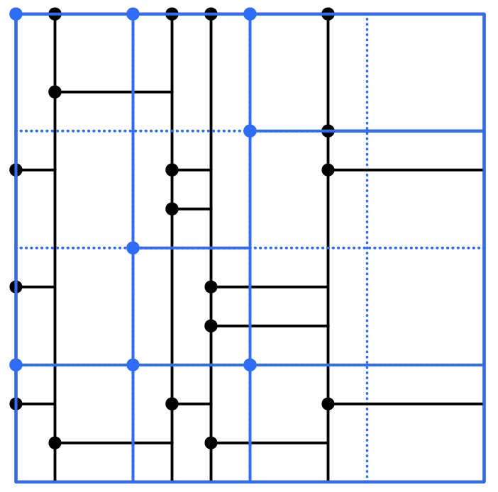
Figure 2. Coupling the square partition defined by the continuous time Poisson process $\Sigma$ (black) with the partition $\Sigma_{n}$, with break points at multiples of $1/n$, for $n=4$. In reality $\Sigma$ has infinitely many parts a.s. Given a blue rectangle in $\Sigma_{n}$ with top left corner $y$ we compare it with the black rectangle in $\Sigma$ with top left corner $x$ where $x$ is the rightmost and then bottom most point across from $y$ in the dashed blue square with top left corner $y$.

Finally for the lower bound note that

$$nk\lVert a_{i}b_{i}-(\Sigma_{a})_{i}\Sigma_{b_{i}}\rVert_{1}=\sum_{j=1}^{\infty}\left\lvert na_{i}\cdot k(b_{i})_{j}-n(\Sigma_{a})_{i}\cdot k(\Sigma_{b_{i}})_{j}\right\rvert\geq\sum_{j=1}^{\infty}\lVert n(\Sigma_{a})_{i}\cdot k(\Sigma_{b_{i}})_{j}\rVert_{\mathbb{Z}}$$

where $\lVert\cdot\rVert_{\mathbb{Z}}$ denotes distance to the nearest integer, since $na_{i}\cdot k(b_{i})_{j}\in\mathbb{Z}$. To handle this term we use a result of Kingman [kingman1975random] that

$$\mathbb{E}_{\Sigma}\sum_{i=1}^{\infty}\phi(\Sigma_{i})=\int_{0}^{1}\phi(t)\frac{1}{t}dt$$

for any nonnegative $\phi$ that makes the right hand side convergent, which can be seen from the Poisson process construction of the Poisson-Dirichlet [arratia2006tale, ignatov1982constant]. Then

$$\psi(x) \coloneqq\mathbb{E}_{\Sigma}\sum_{i=1}^{\infty}\lVert x\cdot k\Sigma_{i}\rVert_{\mathbb{Z}}=\int_{0}^{1}\lVert x\cdot ky\rVert_{\mathbb{Z}}\frac{1}{y}dy\geq\sum_{m=1}^{\left\lfloor kx-1/2\right\rfloor}\int_{m-1/2}^{m+1/2}\frac{\lVert z\rVert_{\mathbb{Z}}}{z}dz$$

$$=\sum_{m=1}^{\left\lfloor kx-1/2\right\rfloor}\int_{m-1/2}^{m}\frac{m-z}{z}dz+\int_{m}^{m+1/2}\frac{z-m}{z}dz=\sum_{m=1}^{\left\lfloor kx-1/2\right\rfloor}m\log\left(\frac{m^{2}}{m^{2}-1/4}\right)$$

$$=\sum_{m=1}^{\left\lfloor kx-1/2\right\rfloor}-m\log\left(1-\frac{1}{4m^{2}}\right)$$

so since $\Sigma_{a},\Sigma_{b_{1}},\Sigma_{b_{2}},\dots$ are iid copies of $\Sigma$

$$nkd_{L^{1}}(C,\mathcal{P}) =\mathbb{E}\sum_{i=1}^{\infty}\psi(n\Sigma_{i})=\int_{0}^{n}\psi(x)\frac{1}{x}dx\geq\sum_{m=1}^{kn-1}-m\log\left(1-\frac{1}{4m^{2}}\right)\int_{\frac{m+1/2}{k}}^{n}\frac{1}{x}dx$$

$$\sim\frac{1}{4}\left(\log(kn)\sum_{m=1}^{kn-1}\frac{1}{m}-\sum_{m=1}^{kn-1}\frac{\log\left(m+1/2\right)}{m}\right)\sim\log^{2}(kn)/8$$

∎

Here is an easy extension to general wreath products. Note that $m$ is now fixed so $\mathcal{B}$ is a finite partition with at most $m$ parts.

Theorem 5.1 (Cycle partition convergence).

Let $\Gamma\subset S_{m}$ be arbitrary. Take $\pi\in\Gamma^{n}\rtimes S_{n}$ uniformly and let $C_{1},C_{2}\dots$ be the cycle lengths in $\pi$. Let $C=\left(\frac{C_{1}}{mn},\frac{C_{2}}{mn},\dots\right)$. Then

$$d_{L^{\infty}}(C,\mathcal{A})\leq 1/n$$

and

$$d_{L^{1}}(C,\mathcal{A})\leq\frac{3(\log n+\gamma)}{n}+O(1/n^{2})$$

where $\mathcal{A}$ satisfies

$$\mathcal{A}=(U\mathcal{B},(1-U)\mathcal{A})$$ (6)

and $\mathcal{B}=\left\{\frac{D_{1}}{m},\frac{D_{2}}{m},\dots\right\}$ is the finite random partition distributed according to cycles $D_{1},D_{2},\dots$ of a uniform permutation from $\Gamma$.

Proof.

The exact same proof as Theorem 1.1 but with $b_{1},b_{2},\dots$ iid distributed according to $\mathcal{B}$. Since $\mathcal{A}=f(\Sigma,\mathcal{B},\mathcal{B},\dots)$ only the coupling $(a,\Sigma_{a})$ is needed. ∎

As an example consider the generalized symmetric group, known as the group of symmetries of the hypercube and which also happens to be important in understanding which permutations commute with each other [diaconis2024poisson].

Example 5.2 (Generalized symmetric group partition).

Consider a random permutation from $C_{m}^{n}\rtimes S_{n}$. Then $\mathcal{B}$ has equal size parts almost surely and $\mathbb{P}\left(\left\lvert\mathcal{B}\right\rvert=\frac{m}{l}\right)=\frac{\phi(l)}{m}$ for $l|m$.

6. Large parts

This section derives recursive equations satisfied by the distribution of the $k$th largest part of general self-similar partitions, extending Theorem 3.1. These include partitions that do not arise as limits of wreath product cycles, and may be of independent interest. Throughout let $\mathcal{P}_{k}$ denote the $k$-th largest part of the partition $\mathcal{P}$. By convention $\mathcal{P}_{j}=\infty$ for nonpositive $j$, $\mathcal{P}_{k}=0$ for any $k>\left\lvert\mathcal{P}\right\rvert$, and $1/0=\infty$.

Theorem 6.1 ($k$-th largest part).

Let $\mathcal{B}$ be a random partition of unity and $\mathcal{A}$ the random partition of unity defined by

$$\mathcal{A}=(U\mathcal{B},(1-U)\mathcal{A})$$

in distribution. Then

$$\phi_{k}(u)\coloneqq\mathbb{P}\left(\mathcal{A}_{k}\leq 1/u\right)=\frac{1}{u}\sum_{j=0}^{k-1}\mathbb{E}_{\mathcal{B}}\int_{(u-1/\mathcal{B}_{j+1})\vee 0}^{u-1/\mathcal{B}_{j}}\phi_{k-j}(y)dy$$

with $\phi_{1}(u)=1$ for $u\in[0,1]$. Equivalently

$$u\phi_{k}(u)=\sum_{j=0}^{k-1}(S_{j}\ast\phi_{k-j})(u)$$

where $S_{j}(x)=\mathbb{P}\left(\mathcal{B}_{j+1}\leq 1/x<\mathcal{B}_{j}\right)$.

Proof.

$$\mathbb{P}\left(\mathcal{A}_{k}\leq 1/u\right) =\mathbb{P}\left((U\mathcal{B},(1-U)\mathcal{A})_{k}\leq 1/u\right)=\mathbb{E}_{\mathcal{B}}\mathbb{P}_{U,\mathcal{A}}\left((U\mathcal{B},(1-U)\mathcal{A})_{k}\leq 1/u\right)$$

$$=\mathbb{E}_{\mathcal{B}}\int_{0}^{1}\sum_{j=0}^{k-1}1_{\mathcal{B}_{j+1}\leq\frac{1}{ut}<\mathcal{B}_{j}}\mathbb{P}\left(\mathcal{A}_{k-j}\leq\frac{1}{u(1-t)}\right)dt$$

$$=\frac{1}{u}\sum_{j=0}^{k-1}\mathbb{E}_{\mathcal{B}}\int_{1/\mathcal{B}_{j}}^{(1/\mathcal{B}_{j+1})\wedge u}\mathbb{P}\left(\mathcal{A}_{k-j}\leq\frac{1}{u-y}\right)dy$$

$$=\frac{1}{u}\sum_{j=0}^{k-1}\mathbb{E}_{\mathcal{B}}\int_{(u-1/\mathcal{B}_{j+1})\vee 0}^{u-1/\mathcal{B}_{j}}\phi_{k-j}(y)dy$$

The second formula follows from Fubini after the third equality and then proceeding similarly. ∎

A similar approach can be used to derive a differential difference equation satisfied by the joint distribution function of the $k$ largest pieces, but this is not pursued here. In cases where $\mathcal{B}$ has a bounded number of parts the expectation formula seems more natural. Combining the above with Theorem 5.1 gives the below.

Corollary 6.2 (Large cycles).

Let $\Gamma\subset S_{m}$ be arbitrary. Take $\pi\in\Gamma^{n}\rtimes S_{n}$ uniformly and let $C_{k}$ be the $k$-th largest cycle. Then

$$\frac{C_{k}}{mn}\stackrel{{\scriptstyle d}}{{\longrightarrow}}\mathcal{A}_{k}$$

where $\phi_{k}(u)\coloneqq\mathbb{P}\left(\mathcal{A}_{k}\leq 1/u\right)$ satisfies the recurrence relations of Theorem 6.1 with $\mathcal{B}_{j}$ the $j$-th largest cycle of a uniform permutation from $\Gamma$.

Taking $\Gamma=S_{1}$, so $\mathcal{B}_{1}=1$ and $\mathcal{B}_{j}=0$ for $j>1$ almost surely, recovers $\phi_{k}=\rho_{k}$ as in [knuth1976analysis], where $\rho_{1}$ is Dickman’s function and $\rho_{k}$ describes the $k$-th largest normalized cycle length. Here is a continuation of Example 5.2.

Example 6.3 (Largest cycle from generalized symmetric group).

Consider $\mathcal{B}=\left\{\frac{l}{m},\frac{l}{m},\dots,\frac{l}{m}\right\}$ with probability $\frac{\phi(l)}{m}$ for $l|m$ ($\phi$ totient). Then the expectation formula gives, for $\psi_{k}(u)\coloneqq\mathbb{P}\left(\mathcal{A}_{k}\leq 1/u\right)$

$$u\psi_{k}(u)=\sum_{l|m}\frac{\phi(l)}{m}\int_{u-m/l}^{u}\psi_{k}(t)dt+\sum_{\begin{subarray}{c}l|m\\ l>m/k\end{subarray}}\frac{\phi(l)}{m}\int_{0}^{u-m/l}\psi_{k-m/l}(t)dt$$

7. Identities and asymptotics

The convolution formula for $k=1$ gives $\phi_{1}(u)=\frac{1}{u}(S_{0}\ast\phi_{1})(u)$ which is exactly the set of integral equations considered in Section 4. Since [granville2001spectrum] actually gives an explicit representation for solutions to such equations we immediately get an expression for the distribution function of the largest part of any self-similar partition. Explicitly, with $S_{0}=\psi_{1}$ the distribution of the largest part of $\mathcal{B}$, then with $\phi_{1}$ as in Theorem 6.1 we have

$$\phi_{1}(u)=\sum_{k=0}^{\infty}\frac{(-1)^{k}}{k!}\int_{\begin{subarray}{c}t_{1},\dots,t_{k}\geq 1\\ t_{1}+\dots+t_{k}\leq u\end{subarray}}\frac{1-\psi_{1}(t_{1})}{t_{1}}\dots\frac{1-\psi_{1}(t_{k})}{t_{k}}dt_{1}\dots dt_{k}$$

The case of $\phi_{1}=\rho$, the Dickman function, is attributed to Ramanujan [andrews2013ramanujan]. The formula is reminiscent of the probability mass function of the number of cycles of a given length in a uniform permutation [goncharov1944some], and both can be proved with inclusion-exclusion. One may also obtain formulas for $\phi_{1}$ by way of Fourier inversion of the Laplace transform, which is easy to compute if one knows the Laplace transform for $\psi_{1}$ (see comments at the end of section 4). It’s possible some of these formulas could be used to obtain asymptotics. We take a different approach here with our running example.

Example 7.1.

Continuing Example 6.3, assuming $u\geq m$ and because $\psi_{1}$ is nonincreasing

$$u\psi_{1}(u) =\sum_{l|m}\frac{\phi(l)}{m}\int_{u-m/l}^{u}\psi_{1}(t)dt\leq\sum_{l|m}\frac{\phi(l)}{m}\frac{m}{l}\psi_{1}(u-m/l)$$

$$=\sum_{l|m}\prod_{p|l}\left(1-\frac{1}{p}\right)\psi_{1}(u-m/l)\leq m\psi_{1}(u-m)$$

where the last inequality is rather loose. Iterating this $\left\lceil u/m\right\rceil$ times gives

$$\psi_{1}(u)\leq\frac{m^{\left\lceil u/m\right\rceil}}{u!_{(m)}}=\frac{m^{\left\lceil u/m\right\rceil}}{u(u-m)(u-2m)\dots}$$

but we conjecture the true decay is much more rapid for large $m$. The term $\sum_{l|m}\frac{\phi(l)}{m}\int_{u-m/l}^{u}\psi_{1}(t)dt$ is the expectation over a random integral of the function’s history, where the amount of time $m/l$ one looks back is sampled proportional to $\phi(l)$. Our upper bound is then the integral over the most history, rounded to simply be the area of a rectangle. However looking back this far is the lowest probability event, with mass only $1/m$, and this bound gets looser as $m$ grows.

Appendix A Convergence of cycle counts

Theorem A.1 (Cycle count convergence).

Pick $\sigma\in S_{k}^{n}\rtimes S_{n}$ uniformly and let $\sigma\sim\prod_{i=1}^{kn}i^{a_{i}(\sigma)}$. Then, as both $k,n\to\infty$, the joint distribution of $\{a_{i}(\sigma)\}_{i=1}^{kn}$ converges (weakly) to the law of $\{A_{i}\}_{i=1}^{\infty}$ with

$$A_{i}=\sum_{kl=i}\sum_{j=1}^{\infty}jX_{l,k,j}$$

where $X_{l,k,j}\sim\operatorname{Poi}\left(\frac{p^{k}_{j}}{l}\right)$ with $p^{k}_{j}$ the Poisson PMF with parameter $1/k$ evaluated at $j$. $\left\{X_{l,k,j}\right\}_{j}\cup\left\{X_{l^{\prime},k^{\prime},j}\right\}_{j}$ are mutually independent if $l\neq l^{\prime}$, but otherwise may be dependent. Consequently

$$\mathbb{E}[A_{i}]=\frac{\sigma_{0}(i)}{i},\quad\operatorname{Var}(A_{i})=\frac{\sigma_{0}(i)}{i}+\frac{1}{i}\sum_{l|i}\frac{1}{l}$$

where $\sigma_{0}(i)$ is the number of divisors of $i$.

First here is a lemma extending Poisson splitting when splitting into countably many processes.

Lemma A.2 (Infinite Poisson splitting).

Let $\sum_{i=1}^{\infty}1_{E_{i}}$ be distributed $\operatorname{Poi}(\lambda)$. Then $\left\{\sum_{i=1}^{\infty}1_{Y_{i}=j}1_{E_{i}}\right\}_{j=0}^{\infty}$ is a countable collection of independent $\operatorname{Poi}(p_{j}\lambda)$ sums where $p_{j}=\mathbb{P}\left(Y_{1}=j\right)$ and $Y_{i}$ are iid with support in $\mathbb{N}_{0}$

Proof.

Let $X=\sum_{i=1}^{\infty}1_{E_{i}}$ and $X_{j}=\sum_{i=1}^{\infty}1_{Y_{i}=j}1_{E_{i}}$. Let $k_{1},\dots,k_{m}\in\mathbb{N}$ be arbitrary, $k=\sum_{i=1}^{m}k_{i}$, and $p=\sum_{j=1}^{m}p_{j}$. Then

$$\mathbb{P}\left(X_{1}=k_{1},\dots,X_{m}=k_{m}\right) =\sum_{n=k}^{\infty}\mathbb{P}\left(X_{1}=k_{1},\dots,X_{m}=k_{m},X=n\right)$$

$$=\sum_{n=k}^{\infty}\frac{e^{-\lambda}\lambda^{n}}{n!}{n\choose k_{1},\dots,k_{m}}p_{1}^{k_{1}}\dots p_{m}^{k_{m}}(1-p)^{n-k}$$

$$=\prod_{j=1}^{m}\frac{e^{-\lambda p_{j}}(\lambda p_{j})^{k_{j}}}{k_{j}!}\sum_{n=k}^{\infty}\frac{e^{-\lambda(1-p)}(\lambda(1-p))^{n-k}}{(n-k)!}$$

$$=\prod_{j=1}^{m}\frac{e^{-\lambda p_{j}}(\lambda p_{j})^{k_{j}}}{k_{j}!}$$

Since this holds for any $m$ we conclude. Indeed taking $m=1$ gives marginal Poisson distribution and arbitrary $m$ gives independence of the countable collection. ∎

Proof of Theorem A.1.

With notation as in Section 5.1, let $E,F^{1},F^{2},\dots$ be independent copies of $\Xi$, $E_{k,i}$ the event that there is a $k$-space starting at $i$ in $E$, and $F^{i}_{k,j}$ the event that there is a $k$-space starting at $j$ in $F^{i}$. Let $Y^{k}_{i}=\sum_{j=1}^{\infty}1_{F^{i}_{k,j}}$, the number of $k$-spaces in $F^{i}$, which is $\operatorname{Poi}(1/k)$ by Ignatov’s theorem [ignatov1982constant]. The coupling and product observation at the start of Section 2 then give that

$$a_{i}\stackrel{{\scriptstyle d}}{{\longrightarrow}}\sum_{\begin{subarray}{c}kl=b\end{subarray}}\sum_{i=1}^{\infty}Y_{i}^{k}1_{E_{l,i}}$$

so it suffices to show that

$$\sum_{\begin{subarray}{c}kl=b\end{subarray}}\sum_{i=1}^{\infty}Y_{i}^{k}1_{E_{l,i}}\overset{d}{=}\sum_{kl=b}\sum_{j=1}^{\infty}jX_{l,k,j}$$

Ignatov’s theorem also says

$$\sum_{i=1}^{\infty}1_{E_{l,i}}\overset{d}{=}X_{l}$$ (7)

where $X_{l}\sim\operatorname{Poi}(1/l)$ independently. By Fubini we have

$$\sum_{\begin{subarray}{c}kl=b\end{subarray}}\sum_{i=1}^{\infty}Y_{i}^{k}1_{E_{l,i}}=\sum_{\begin{subarray}{c}kl=b\end{subarray}}\sum_{j=0}^{\infty}j\sum_{i=1}^{\infty}1_{Y^{k}_{i}=j}1_{E_{l,i}}$$

Now by infinite Poisson splitting

$$\left(\sum_{i=1}^{\infty}1_{Y^{k}_{i}=j}1_{E_{l,i}}\right)_{j=0}^{\infty}\overset{d}{=}\left(X_{l,k,j}\right)_{j=0}^{\infty}$$

and are independent across $l,j$. Indeed the sequences of random variables $\left\{Y^{k}_{i}\right\}_{i=1}^{\infty}$ are iid across $i$, so splitting holds. The expectation and variance formulas are straightforward computations using the mean and variance of a Poisson twice each. ∎

References

- \ProcessBibTeXEntry \ProcessBibTeXEntry \ProcessBibTeXEntry \ProcessBibTeXEntry \ProcessBibTeXEntry \ProcessBibTeXEntry \ProcessBibTeXEntry \ProcessBibTeXEntry \ProcessBibTeXEntry \ProcessBibTeXEntry \ProcessBibTeXEntry \ProcessBibTeXEntry \ProcessBibTeXEntry \ProcessBibTeXEntry \ProcessBibTeXEntry \ProcessBibTeXEntry \ProcessBibTeXEntry \ProcessBibTeXEntry \ProcessBibTeXEntry \ProcessBibTeXEntry \ProcessBibTeXEntry \ProcessBibTeXEntry \ProcessBibTeXEntry \ProcessBibTeXEntry