Cold dark gas in Cygnus X: The first large-scale mapping of low-frequency carbon recombination lines

Abstract

Understanding the transition from atomic gas to molecular gas is critical to explain the formation and evolution of molecular clouds. However, the gas phases involved, cold H i and CO-dark molecular gas, are challenging to directly observe and physically characterize. We observed the Cygnus X star-forming complex in carbon radio recombination lines (CRRLs) at 274–399 MHz with the Green Bank Telescope at 21 pc (48^′) resolution. Of the 30 deg² surveyed, we detect line-synthesized C273$\alpha$ emission from 24 deg² and produce the first large-area maps of low-frequency CRRLs. The morphology of the C273$\alpha$ emission reveals arcs, ridges, and extended possibly sheet-like gas which are often on the outskirts of CO emission and likely transitioning from H i-to-H₂. The typical angular separation of C273$\alpha$ and ¹³CO emission is 12 pc, and we estimate C273$\alpha$ gas densities of $n_{H}\approx 40-400$ cm^-3. The C273$\alpha$ line profiles are Gaussian and likely turbulent broadened, spanning a large range of FWHM from 2 to 20 km s^-1 with a median of 10.6 km s^-1. Mach numbers of the fall within 10–30. The turbulent timescale is relatively short, 2.6 Myr, and we deduce that the turbulent pressure likely dominates the evolution of the C273$\alpha$ gas. Velocity differences between C273$\alpha$ and ¹³CO are apparent throughout the region and have a typical value of 2.9 km s^-1. Two regimes have emerged from the data: one regime in which C273$\alpha$ and ¹³CO are strongly related (at $N(H)\approx 4\times 10^{21}$ cm^-2), and a second, in which C273$\alpha$ emits independently of the ¹³CO intensity. In the former regime, C273$\alpha$ may arise from the the envelopes of massive clouds (filaments), and in the latter, C273$\alpha$ emits from cold clumps in a more-diffuse mix of H i and H₂ gas.

1 Introduction

Understanding the transition from atomic gas to molecular gas is critical to explain the formation and evolution of molecular clouds. There are two main phases of gas directly involved in the H i-to-H₂ transition, cold H i and CO-dark molecular gas. They are often referred to as cold “dark” gas, since they are challenging to directly observe with typical tracers, H i 21 cm and CO rotational transitions, leading to a dearth of knowledge around the formation of molecular gas in galaxies. Cold dark gas is estimated to make up a considerable fraction of the Galaxy’s interstellar medium (ISM) mass (Grenier et al., 2005; Remy et al., 2018; Busch et al., 2021; Murray et al., 2020; Marchal et al., 2024).

On cloud-scales, the H i-to-H₂ transition marks where gas is converted from a mostly atomic state to mostly molecular. The gas density, far-ultraviolet (FUV; 6-13.6 eV) radiation, and dust properties describe the column densities (or $A_{V}$) where and how rapidly this transition occurs; the H i-to-H₂ transition typically takes place at $A_{V}=0.4-1$ from models (van Dishoeck & Black, 1986; Wolfire et al., 2010; Sternberg et al., 2014) and observations (Imara & Burkhart, 2016; Schneider et al., 2023). H₂ formation occurs via catalytic reactions on the surfaces of interstellar dust grains. The H₂ formation rate, $R_{\mathrm{H}_{2}}$, is primarily dependent on gas density via the relation $R_{\mathrm{H}_{2}}\propto n_{\mathrm{HI}}\,n_{\mathrm{H}}\,T_{e}^{1/2}\,Z$, where $n_{\mathrm{H}}$ is the number density of hydrogen nuclei, $n_{\mathrm{H\,I}}$ is the number density of atomic hydrogen H i, $T_{e}$ is the electron temperature, and $Z$ is the metallicity (for a review, see Wakelam et al., 2017). However, the net formation or destruction of H₂ and the cloud structure where this occurs depends on the far-ultraviolet (FUV; 6–13.6 eV) radiation field and dust properties, in addition to gas density (e.g., Wolfire et al., 2010; Sternberg et al., 2014). The ambient radiation field in the ISM rapidly photo-dissociates H₂ and also heats the gas through photoelectric heating. Dust helps to shield and attenuate FUV radiation. When the H₂ opacity to FUV radiation becomes high enough such that self-shielding of H₂ is efficient, the abundance of H₂ rapidly increases. Because carbon has a lower ionization potential (IP = 11.26 eV) than hydrogen (IP = 13.6 eV), carbon may be singly ionized in regions where hydrogen is predominantly molecular. CO, the workhorse tracer of molecular clouds (e.g., Bolatto et al., 2013; Heyer & Dame, 2015), reaches the abundances required to self-shield, and thus become observable, only deeper into the cloud.

In a galaxy’s ecosystem, molecular gas forms in bulk from the compression, cooling, and fragmentation of the ISM. There are a number of mechanisms proposed to form giant molecular clouds (for a review see Dobbs et al., 2014; Chevance et al., 2023), massive gravitationally-bound agglomerations of molecular gas. The mechanisms that regulate the net formation of H₂ include turbulence, shocks, gas flows, the gravitational stability of a molecular cloud, the ISM pressure and weight, and magnetic field strength.

The gas phases involved in the H i-to-H₂ transition are difficult to observe. H i from warm ($T\sim 7000$ K) gas dominates the main H i 21 cm observable, and cold H i ($T\sim 70$ K; Heiles & Troland, 2003) is observable towards select (i.e., often nearby, high-latitude) lines-of-sight, or through H i self-absorption (HISA) when illuminated by a warm-H i background component (Heeschen, 1955). These studies have provided foundational insights into diffuse and translucent cloud conditions (McClure-Griffiths et al., 2023). To infer the presence of cold dark gas and investigate its properties, decomposing far-IR dust emission (e.g., Planck Collaboration et al., 2011), gamma-ray emission (e.g., Grenier et al., 2005), and [C ii] 158 $\mu$m emission (e.g., Pineda et al., 2013; Tang et al., 2016) into the multi-phase ISM components from which they arise has also been employed. Recently strides have been made in directly observing the dark components, with [C ii] especially in star forming environments (Beuther et al., 2014; Schneider et al., 2023; Bonne et al., 2023) and with quasi-thermal OH emission (Busch et al., 2019, 2021).

Carbon radio recombination lines (CRRLs) at low-frequencies ($<1$ GHz) strongly complement these dark gas probes. CRRLs arise from high principal quantum number transitions ($\mathsf{n}\gtrsim 26$) in C⁺ gas, where carbon is predominantly singly ionized. At low radio frequencies ($<$1 GHz, $\mathsf{n}\gtrsim 187$), CRRL emission is enhanced due to stimulation and dielectronic capture (Shaver, 1975; Watson et al., 1980). Atomic physics modeling shows low-frequency CRRLs traces gas with temperatures of 20–100 K and densities $n_{e}=0.01-0.1$ cm^-3 ($n_{\mathrm{H}}=100-1000$ cm^-3) (Walmsley & Watson, 1982; Payne et al., 1994; Salgado et al., 2017a). The warmer and denser conditions of C⁺ gas found in classic, dense photo-dissociation regions (PDRs) are observed with high-frequency CRRL emission but not at low-frequencies due to increased pressure broadening, decreased stimulation and fainter background continuum, and optically thick free-free continuum of associated regions.

Low-frequency CRRL observations are excellent probes of the H i-to-H₂ transition because they trace the density and temperature regime where the transition takes place. However, they have largely been underutilized due to a lack of high-resolution and high-sensitivity telescopes at the relevant frequencies. Pioneering work with low-frequency CRRLs have shown that they are ubiquitous in large (2^∘–110^∘) beams where background continuum is bright (Anantharamaiah, 1985; Erickson et al., 1995; Roshi & Anantharamaiah, 1997; Kantharia & Anantharamaiah, 2001; Roshi et al., 2002; Vydula et al., 2023), for example towards the Inner Galaxy. Roshi et al. (2002) found CRRL emission at 327 MHz to resemble the radial extent of intense ¹²CO emission in our Galaxy. Roshi & Kantharia (2011) used Ooty Telescope 327 MHz survey data associated with the Riegel-Crutcher Cloud, identified that the narrow CRRL components are coincident with HISA features, estimated H₂ formation rates which far exceeded dissociation rates, and thereby showed that CRRLs trace gas in the process of forming molecular gas.

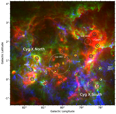
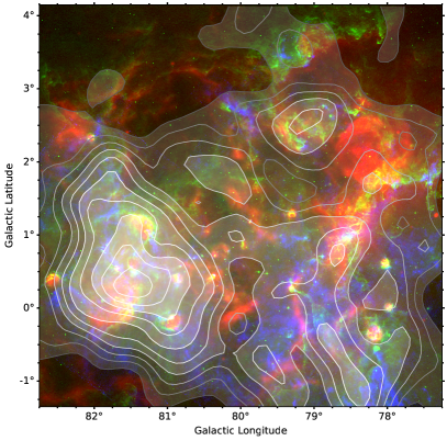
Figure 1: RGB compilation in the Cygnus X region covering the footprint that we surveyed; in red is the CGPS 1.4 GHz continuum (Taylor et al., 2003), green is MSX 8 $\mu$m PAH emission Schneider et al. (2006), and blue is ¹³CO (1-0) tracing (some of the) molecular gas (Schneider et al., 2010). Left: The numbers enclosed by a circle in black indicate the ‘DR’ continuum sources identified in 5 GHz observations by Downes & Rinehart (1966), which are mostly thermal H ii regions, except for DR3 and DR4 that make up the supernova remnant $\gamma$-Cygni. Dotted circles show the Cyg OB2 association and open clusters NGC 6910 and NGC 6913. The region at $\ell>80$^∘ commonly referred to as Cyg X North and at $\ell<80$^∘ (also typically at lower latitudes) as Cyg X South are also indicated. Right: Contours of velocity-integrated C273$\alpha$ (moment 0), drawn at $[3,5.5,8,...28]\sigma$. C273$\alpha$ is detected from 75% of the mapped region.

Recently, higher resolution (arcsec to arcmin) studies of low-frequency CRRLs have been enabled, thanks to upgraded receivers and high-resolution telescopes at low frequencies (Salas et al., 2017; Oonk et al., 2017; Salas et al., 2018, 2019; Chowdhury & Chengalur, 2019; Roshi et al., 2022). Detailed studies of gas in the Perseus Arm along the line-of-sight towards the Cassiopeia A (Cas A) supernova remnant find CRRL emitting layers to trace the surface of a molecular cloud (Oonk et al., 2017; Salas et al., 2018). Chowdhury & Chengalur (2019) used GMRT 430 MHz observations and find clumps of CRRL emission on scales of $<0.3$ pc embedded in larger-scale ($\geq 7$ pc) diffuse emission. In the Orion star-forming region, CRRLs used in conjunction with [C ii] 158 $\mu$m provided key physical properties to anchor models of photodissociation regions (Salas et al., 2019).

Although large-beam surveys are highly valuable, they have so far not produced maps of low-frequency CRRL emission. Only gas in front of the extremely bright, $S_{100~\mathrm{MHz}}\sim 10^{4}$ Jy, Cas A has been resolved and mapped over the 8^′ diameter (0.014 deg² area) supernova remnant (Kantharia et al., 1998; Salas et al., 2018; Chowdhury & Chengalur, 2019).

In this article, we present the results of CRRL observations at 274–399 MHz using the Green Bank Telescope (GBT) in a 30 deg² area covering the Cygnus X star forming region. We use these observations to investigate the H i-to-H₂ transition (or vice versa) in the formation or destruction of molecular clouds. To our knowledge, this is the first mapping of CRRLs arising from cold, diffuse gas that is larger than $0.014$ deg². The high surface brightness of the radio continuum elevates the line intensities of the stimulated CRRLs. The gas content and stellar activity in Cygnus X allows us to characterize the H i-to-H₂ transition in actively forming molecular gas (Schneider et al., 2023; Bonne et al., 2023) and in the presence of an elevated radiation field.

2 Overview of the region

Cygnus X is a nearby (approximately 1.5 kpc) massive star-forming complex that spans more than 6 degrees in size (see Figure 1). Cygnus X hosts more than 170 massive OB stars (Le Duigou & Knodlseder, 2002; Comerón & Pasquali, 2012; Wright et al., 2015; Berlanas et al., 2018; Comerón et al., 2020; Quintana & Wright, 2021) — some of which are surrounded by bright H ii regions (e.g., Downes & Rinehart, 1966, see ‘DR’ source IDs in Figure 1) — a large number of actively forming stars (Motte et al., 2007; Beerer et al., 2010; Bontemps et al., 2010; Ortiz-León et al., 2021), and stellar remnants of supernovae and pulsars (e.g., Ladouceur & Pineault, 2008). Cyg OB2 ($d\sim 1.4-1.7$ kpc; Berlanas et al., 2019; Cantat-Gaudin & Anders, 2020; Quintana & Wright, 2021), a prominent association of stars in the heart of the region, has a stellar mass of around $2\times 10^{4}$ $\rm M_{\odot}$ (Wright et al., 2015) and age 3–5 Myr (Wright et al., 2010; Berlanas et al., 2020). Cyg OB2 bathes the region in a high UV radiation field ($G_{0}\gtrsim 5-1000$; e.g., Schneider et al., 2016) and has had profound impacts by triggering star formation (Schneider et al., 2016; Deb et al., 2018), photo-evaporating cold clouds (Wright et al., 2012; Emig et al., 2022), and through its stellar winds (Ackermann et al., 2011; Abeysekara et al., 2021).

The Cygnus X region contains an abundance of molecular gas (e.g., Schneider et al., 2006), with two main concentrations of emission generally referred to as Cyg X North ($M_{\mathrm{H_{2}}}\approx 3\times 10^{5}$ $\rm M_{\odot}$) and Cyg X South ($M_{\mathrm{H_{2}}}\approx 5\times 10^{5}$ $\rm M_{\odot}$), with a cleared medium in between aligned with Cyg OB2 (see Figure 1). The molecular clouds in Cyg X North that are primarily associated with DR21 and W75N may be interacting (Dickel et al., 1978; Dobashi et al., 2019; Schneider et al., 2023; Bonne et al., 2023); a cloud-cloud collision has also been hypothesized for clouds in Cyg X South (Schneider et al., 2006). A foreground cloud, part of the Great Cygnus Rift ($d\sim 600-800$ pc; e.g., see review in Uyaniker et al., 2001), also contributes to some emission in this direction.

In this article, we assume the distance to the Cygnus X clouds is $1.5\pm 0.2$ kpc (e.g., Rygl et al., 2012), for which 1^′ $=0.44\pm 0.06$ pc.

3 Data

3.1 GBT Observations and Data Reduction

We mapped a $5.5\times 5.5$ sq. degree ($144\times 144$ sq. pc) region centered on $(\ell,b)=(80\text{$^{\circ}$},1.4\text{$^{\circ}$})$ using the $342$ MHz prime focus receiver (Rcvr_342) on the 100 m Robert C. Byrd Green Bank Telescope (GBT; Prestage et al., 2009). The observations were carried out between April 16, 2021 and May 23, 2021 as part of project GBT21A-292, sessions 14 to 23. Radio recombination line transitions C255$\alpha$ through C282$\alpha$ at 292 – 394 MHz were covered.

The observations used the Versatile GBT Astronomical Spectrometer (VEGAS; Prestage et al., 2015) in spectral line mode to transform the raw voltages into spectra. We observed using the total power mode, firing a noise diode of $\approx 10\%$ of the receiver temperature ($20$–$70$ K) every other integration. We split the frequency range covered by the receiver into seven spectral windows, each $23.44$ MHz wide and with $2^{15}$ channels $0.7$ kHz wide (VEGAS mode $10$). We recorded the linear orthogonal auto-cross correlation products, XX & YY, and used an integration time of $\approx 1.9$ s.

At the start of observing sessions 14, 15, 16 and 19, between April 16, 2021 and May 21, 2021, we determined pointing corrections by observing a bright point-like 3C source (3C295 or 3C48). In general the pointing corrections were smaller than $1\arcmin$, less than $3\%$ of the half power beam width at the highest RRL frequency observed ($31\arcmin$ at $399.14$ MHz for the C$254\alpha$ RRL). During these same sessions we also observed the bright point-like 3C source using position switching to determine the equivalent temperature of the noise diode. We use the flux density scale of Perley & Butler (2017) and adopt an aperture efficiency of $0.71$ for the GBT. Given the small pointing offsets and stability of the temperature of the noise diodes, we decided not to derive pointing corrections nor observe a flux calibrator during other observing sessions.

To calibrate the data we used custom Python data reduction scripts. We follow the formalism described in Winkel et al. (2012), that is, we perform a frequency dependent calibration, as opposed to the default behavior offered by GBTIDL (Marganian et al., 2013).

The first step in our data reduction is to find the gain, including a second order term (see e.g., Salas et al., 2019), using continuum maps for the region. The continuum maps are derived for the central frequency of each spectral window using the methods described in Emig et al. (2022). Then, we split each spectral window into $1000$ km s^-1 sub-windows centered on the hydrogen radio recombination lines (HRRLs). We calibrate each sub-window to antenna temperature applying the previously derived gain, and removing the contribution from the noise diode for the integrations where it was on. Then, we remove the continuum and baseline by fitting an order $11$ polynomial to line free-channels. The line free-channels are defined as being more than $50$ km s^-1 away from the brightest RRL in each sub-window, the HRRLs. To remove radio frequency interference (RFI) we run AOFlagger (Offringa et al., 2012) on each continuum subtracted sub-window. This calibration is performed for each observing session and by treating each polarization independently.

The next step in our data reduction is line stacking. We start by selecting the sub-windows, i.e., lines, that will make it into a stack. For each observing session, we visually inspect the calibrated spectra, one for each CRRL and polarization, and select those that show a smooth bandpass (i.e., can be modeled using a polynomial), show no significant leftover RFI, and have less than $30$% of the data flagged. The selected lines are interpolated to a common velocity grid, with $1200$ channels $0.5$ km s^-1 wide. The interpolated CRRL spectra for a single polarization are averaged together using $T_{\rm{sys}}^{2}/\Delta t$ as weights, with $T_{\rm{sys}}$ the system temperature and $\Delta t$ the integration time. We compare the stacks in both polarizations and look for any spurious features. If the stacks in both polarizations agree, then we repeat the stacking process using both polarizations. We found no instances where both polarizations disagreed by more than their noise. After this step we are left with one set of averaged CRRL spectra for each observing session.

We gridded the averaged CRRL spectra for each observing session using the gbtgridder. During the gridding process we use a Gaussian function as the interpolation kernel with a width equal to the half power beam width of the GBT at the frequency of the lowest CRRL included in the stacks. Finally we averaged together all the cubes from the different observing sessions. This results in a single CRRL cube, which also contains HRRL emission.

We then divide the line intensity, $T_{\mathrm{L}}$, at each voxel of the cube by the intensity of the continuum, $T_{\mathrm{C}}$, creating a line-to-continuum ratio, $T_{\mathrm{L}}/T_{\mathrm{C}}$, data cube. We constructed the continuum image at 321.6 MHz following the methods described in Emig et al. (2022). As we describe in Section 4, CRRLs dominated by stimulated emission have an optical depth equal to the line-to-continuum ratio, $\tau_{\mathrm{L}}\approx-T_{\mathrm{L}}/T_{\mathrm{C}}$, resulting in the line-to-continuum ratio being directly proportional to the physical quantities of interest (Shaver, 1975; Salgado et al., 2017b). We use the $T_{\mathrm{L}}/T_{\mathrm{C}}$ data cube to present our observational results.

The line-synthesized data cube has an effective frequency of 321.6 MHz corresponding to an effective principal quantum number of C273$\alpha$. The beam FWHM is 48.3^′ and the typical noise is $\sigma_{T_{L}/T_{C}}=1.9\times 10^{-4}$ with a 0.5 km s^-1 channel resolution. We constructed a 3D estimate of the noise at each voxel, described in Appendix A.

Throughout this article, we analyze results from the $T_{\mathrm{L}}/T_{\mathrm{C}}$ data cube and often refer to this simply as C273$\alpha$ emission.

3.2 Ancillary Data

¹³CO. We compare C273$\alpha$ emission with a bulk tracer of molecular gas, ¹³CO (1–0) at 110.20 GHz. The opacity of ¹³CO is less than ¹²CO (1-0) and with the deep sensitivity of the observations ($\sim 0.25$ K), the emission is sensitive to even the low column densities of outer cloud layers. Observations kindly provided by the Milky Way Imaging Scroll Painting (MWISP) project (Su et al., 2019; Zhang et al., 2024). These observations cover the entire region mapped by our GBT observations at 15^′ angular and 0.17 km s^-1 velocity resolutions.

In Figure 1, we also show high resolution (48^′′) ¹³CO mapped by the Five College Radio Astronomy Observatory (FCRAO) 14 m telescope (Schneider et al., 2010, 2011) with a noise of 0.2 K at 0.1 km s^-1 channel resolution.

¹²CO. We compare C273$\alpha$ emission with ¹²CO (1–0) emission at 115.27 GHz from molecular gas. We use ¹²CO observations mapped over our full survey region by Leung & Thaddeus (1992) and Dame et al. (2001) with the Center for Astrophysics Millimeter-Wave Telescope. These ¹²CO data have a native beam size of 8.7^′ and noise of 0.12 K at 0.65 km s^-1 channel resolution.

8 $\mu$m. 8 $\mu$m emission mainly traces UV-heated small grains and polycyclic aromatic hydrocarbons (PAHs) in PDRs where the gas is typically in an atomic state. In Figure 1, we compare Midcourse Space Experiment (MSX; Price et al., 2001) 8.3 $\mu$m emission that has an angular resolution of 20^′′ (see Schneider et al., 2006).

H i 21 cm. Spectra of H i 21 cm emission are obtained from the HI4PI Survey with the Effelsberg telescope at 16.2^′ resolution and 43 mK sensitivity in 1.3 km s^-1 channels (HI4PI Collaboration et al., 2016).

RRLs at 5.8 GHz. 5.8 GHz RRL observations from the GBT taken with the same observational setup and data reduction as that of the GBT Diffuse Ionized Gas Survey (GDIGS; Anderson et al., 2021) are used to compare RRL intensities at different frequencies. The data have a native spatial resolution of 2.65^′ and a spectral resolution of 0.5 km s^-1. Compared to GDIGS, the Cygnus X data were taken with less time per pointing, resulting in higher spectral noise, 28 mK versus $\sim 10\,$mK.

1.4 GHz continuum from CGPS. We plot 1.420 GHz continuum emission in this region as observed by the Canadian Galactic Plane Survey (CGPS Taylor et al., 2003) in Figure 1. We convolved and stitched the survey data products as in Emig et al. (2022) to a common resolution of 2′. The standard deviation in a relatively low emission region of the image is $\sigma=0.03$ K (0.7 mJy beam^-1).

4 Description of Low-Frequency Carbon Recombination Line Emission

The solution to the radiative transfer equation for the brightness of a CRRL (Shaver, 1975), from upper level $n+1$ to lower level $n$, i.e., an $\alpha$ transition for which $\Delta n=1$, is, in the optically thin limit:

$$T_{\mathrm{C}n\alpha}\approx\tau^{*}_{\mathrm{C}n\alpha}\left(b_{n+1}T_{e}-b_{n}\beta_{n}T_{o}\right)$$ (1)

where $T_{\mathrm{C}n\alpha}$ is the C$n\alpha$ line temperature, $T_{e}$ is the electron temperature, $T_{o}$ is the continuum background temperature, $b_{n(+1)}$ and $\beta_{n}$ are the departure coefficients which measure the deviation of the level populations from LTE values, and $\tau^{*}_{\mathrm{C}n\alpha}$ is the LTE line optical depth as

$$\tau^{*}_{\mathrm{C}n\alpha}=2.042\times 10^{-6}\left(\frac{EM_{C^{+}}}{\rm{cm^{-6}~pc}}\right)\left(\frac{T_{e}}{\rm{K}}\right)^{-2.5}\left(\frac{\rm{Hz}}{\Delta\nu}\right)$$ (2)

where $EM_{\mathrm{C^{+}}}$ is the emission measure $EM_{\mathrm{C^{+}}}=\int n_{e}n_{\mathrm{C^{+}}}d\ell$ and $\Delta\nu$ is the line width.

Spontaneous emission, the $b_{n+1}T_{e}$ term in Equation 1, typically dominates high-frequency CRRLs, where background continuum, $T_{o}$, is faint and the $b_{n}\beta_{n}$ coefficients are small. Stimulated emission, the $b_{n}\beta_{n}T_{o}$ term in Equation 1, typically dominates low-frequency CRRLs, where both $T_{o}$ and the departure coefficients, $b_{n}\beta_{n}$, take on large values.

When the background continuum term dominates and the CRRL emission is primarily stimulated, Equation 1 becomes,

$$T_{\mathrm{C}n\alpha}\approx-\tau^{*}_{\mathrm{C}n\alpha}b_{n}\beta_{n}T_{C}$$

$$\approx-\tau_{\mathrm{C}n\alpha}T_{C}$$ (3)

where $\tau_{\mathrm{C}n\alpha}$ is the observed non-LTE optical depth, and arriving at the standard relation (Salgado et al., 2017b),

$$\frac{\int T_{L}\Delta\nu}{T_{C}}\approx 2.042\times 10^{-6}\,\mathrm{Hz}\,(-b_{n}\beta_{n})\left(\frac{EM}{\rm{cm^{-6}~pc}}\right)\left(\frac{T_{e}}{\rm{K}}\right)^{-2.5}$$ (4)

where the departure coefficients, $b_{n}\beta_{n}$, take on negative values for lines observed in emission and are themselves dependent upon electron temperature, density, and the radio-continuum radiation field (e.g., Salgado et al., 2017a).

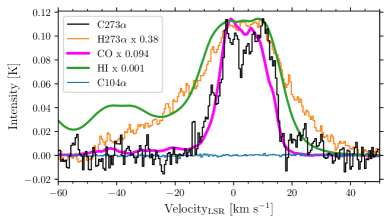
Figure 2: Spatially-averaged line emission of the survey region. The CRRL 322 MHz temperature brightness spectrum of the effective C273$\alpha$ line, which is the spatial average over the entire mapped region. Spatially-averaged spectra of additional gas phases have been normalized to match the peak of C273$\alpha$; ¹²CO (Dame et al., 2001) traces the molecular phase, H i 21 cm (HI4PI Collaboration et al., 2016) traces the atomic phase, and H273$\alpha$ (these data) traces diffuse ionized gas. We also show the non-detection of C$104\alpha$ from GDIGS 5.8 GHz observations (Anderson et al., 2021), emphasizing the stimulated nature of the C273$\alpha$ 321.6 MHz observations.

Figure 2 shows the spatially-averaged line temperature of the 322 MHz C273$\alpha$ in the survey region. C273$\alpha$ peaks at about $T_{L}\approx 0.1$ K. In comparison, the spectrum of 5.8 GHz CRRLs, effectively C104$\alpha$, extracted from the same area in GDIGS observations (Anderson et al., 2021) is not detected with a 3$\sigma$ upper limit of $T_{L}<0.0018$ K. Stimulated line emission is directly proportional to the continuum temperature (Equation 3), and in this region, the continuum is largely $T_{C}\propto\nu^{-2.1}$, (Wendker et al., 1991; Xu et al., 2013; Emig et al., 2022), except towards the supernova remnant where steeper indices are observed. For stimulated emission, the expected line temperature at 5.8 GHz would be $\sim$0.2 mK, as calculated by $T_{L}(5.8\,\mathrm{GHz})\propto T_{L}(322~\mathrm{MHz})\cdot\nu^{-2.1}\approx 100~\mathrm{mK}\cdot(5800/322)^{-2.1}\approx 0.2$ mK, which is consistent with the GDIGS non-detection of $T_{L}(5.8\,\mathrm{GHz})<1.8$ mK. Whereas for spontaneous emission, $T_{L}\propto T_{e}$ and the line temperature is expected to stay within a factor of two from 322 MHz to 5.8 GHz, for $b_{n}$ values that are typically between 0.3–2 (Salgado et al., 2017a). This is inconsistent with the observed line intensities. The spectral line energy distribution (SLED) of the CRRLs therefore indicates that the 322 MHz CRRLs are dominated by stimulated emission.

5 C273$\alpha$ Emission Properties

The observed C273$\alpha$ emission is likely dominated by stimulated emission (Section 4) and is therefore described by Equations 3 & 4. Since the line-to-continuum ratio is directly proportional to the physical properties of the emission, we will present the results in terms of a line-to-continuum ratio $T_{\mathrm{L}}/T_{\mathrm{C}}$ data cube throughout the paper, as is commonly done for low-frequency CRRLs (e.g. Kantharia & Anantharamaiah, 2001; Roshi et al., 2002). While we may refer to the emission simply as C273$\alpha$ emission, it should be taken to mean $T_{\mathrm{L}}/T_{\mathrm{C}}$.

5.1 Velocity-Integrated C273$\alpha$ Map

In Figure 1, we show the velocity-integrated C273$\alpha$ emission (Moment 0) that has been integrated over -10 to 14 km s^-1. The velocity-integrated C273$\alpha$ emission shows that C273$\alpha$ is detected throughout most of the region, having emission with a significance greater than $3\sigma$ ($5\sigma$) over 24.1 (20.3) deg². The elongated and filament-like features seen in the channel maps (Figure 3) are also apparent in the Moment 0 map. Generally, the brightest C273$\alpha$ emission is coincident with Cyg X North, the region of the highest star formation rate surface density that is young and active.

We do not show maps of the intensity-weighted central velocity (Moment 1) or the intensity-weighted velocity dispersion (Moment 2). The data have relatively low signal-to-noise ratios and thus do not produce reliable and meaningful higher order Moment calculations (Teague, 2019).

5.2 C273$\alpha$ Channel Maps

Channel maps of C273$\alpha$ are shown in Figure 3. For visual aid, we mark the locations of well-known radio continuum sources, first cataloged by Downes & Rinehart (1966) at 5 GHz and 10.8^′ resolution. C273$\alpha$ emission appears both extended and elongated throughout most of the channel maps. The size scales of emission range from a fraction of a beam, $\sim$16 ^′ (8 pc), to resolved extensions more than 3^∘ (80 pc) across. Ridges and arcs can be seen in channel 1.3 km s^-1 surrounding DR 9/12/13, in 3.3 km s^-1, in 6.3 km s^-1, in 7.3 km s^-1 bridging DR 22 and 23, in 8.3 km s^-1 upwards from DR 20, and in 11.3 km s^-1 forming an arc in the Western half of the map.

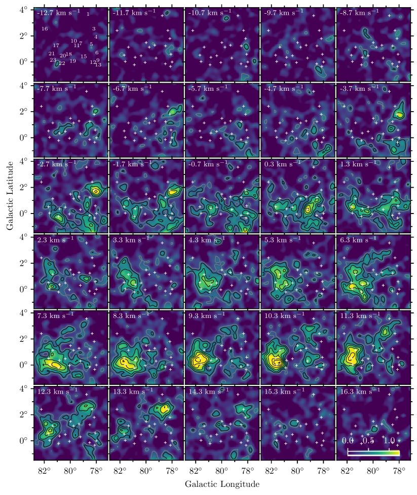
Figure 3: Channel maps of C273$\alpha$. Each channel map has been integrated over 2 channels, equivalent to 1 km s^-1. The central velocity of the map is shown in its top left corner. In the first channel, numbers indicate the DR identifications (Downes & Rinehart, 1966); these sources are marked with a “+” in subsequent channel maps. The color bar, shown in the last channel, indicates the magnitude of $T_{\mathrm{C}273\alpha}/T_{\mathrm{C}}$ in units of 10^-3, and the color scale is the same for all maps. Gray contours are drawn at 3$\sigma$ and black contours are drawn at $[4,6,8,10,12,14]\sigma$ where $\sigma\approx 1.9\times 10^{-4}$.

Bright C273$\alpha$ emission peaks close to DR4, the southern edge of the supernova remnant (SNR) $\gamma$-Cygni, from channels -3.7 km s^-1 to -1.7 km s^-1. The SNR is likely interacting with the ISM (e.g., Ladouceur & Pineault, 2008). Roshi et al. (2022) analyzed RRL emission at 321 MHz within a single GBT beam in this location and found relatively bright carbon RRL emission, being equal in peak intensity to that of hydrogen RRLs at the same frequency. They argued for the CRRLs being emitted in a cold ($T=20-200$ K) and dense ($n_{e}=1.4-6.5$ cm^-3) layer, likely compressed by a shock. Bright CRRL emission also appears towards DR3, the northern edge of the SNR, at 13.3 km s^-1. We discuss emission surrounding the $\gamma$-Cygni SNR in more detail in Section 7.2.

Notably, there is an elongated ridge of emission, peaking coincidentally with DR15 in the 0.3 km s^-1 channel map. At velocities $\gtrsim 3$ km s^-1, Cyg X North dominates the brightest emission in the region, most prominently overlapping spatially with DR 17, 20, 21, 22, and 23. Emission in this region also appears filament or ridge-like at times. Elongated and filamentary-like structure is similarly seen, for example in the Chamaeleon-Musca filament (Bonne et al., 2020) and in the diffuse ISM (for a review see Hacar et al., 2023).

5.3 C273$\alpha$ Spectra and Line Fits

Figure 2 shows line emission from multiple tracers averaged over the full area of the survey region. In this Figure, C273$\alpha$ is presented in terms of a line brightness in units of K, the only instance where we do not show it in terms of $T_{L}/T_{C}$. Most emission between about -20 and 20 km s^-1 in Figure 2 is attributed to clouds in the Cygnus X region forming a coherent complex. Only some velocity ranges can be attributed to emission from the Cygnus rift at distances $<1$ kpc. Emission at -40 km s^-1 is from the Perseus Arm much further away.

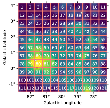
Figure 4: Aperture locations (salmon colored grid lines) and IDs (white number) for the extracted spectra shown in Figure 5.

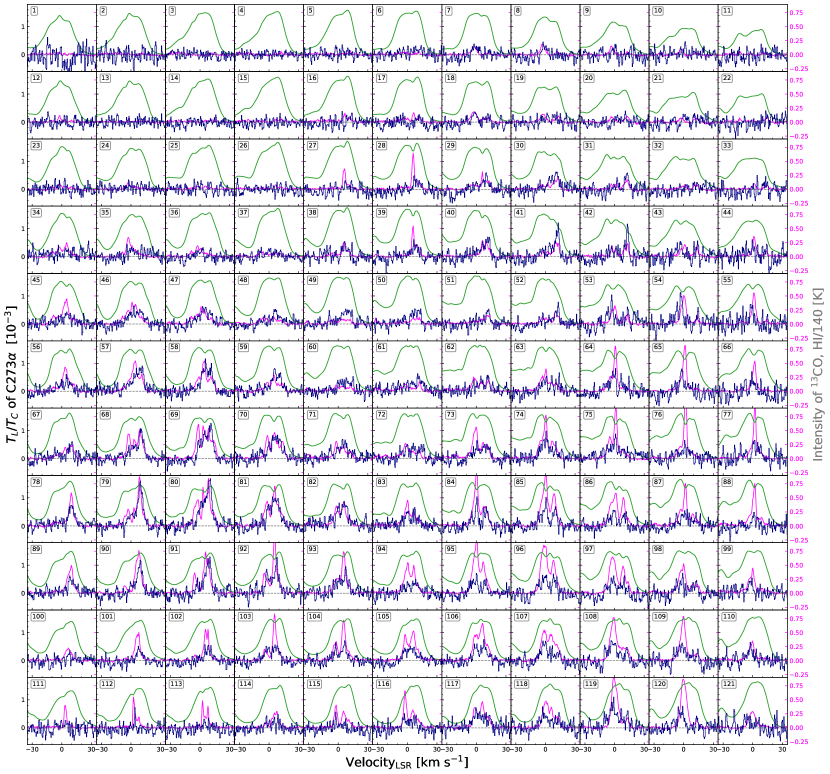
Figure 5: Multi-phase spectra over the mapped region. C273$\alpha$ emission is dark blue, ¹³CO emission is in magenta, and H i 21 cm is green. The aperture ID is shown in a box in the upper-left corner of each spectrum. The y-axis on the right indicates the intensity in units of K for the ¹³CO spectra and for H i spectra that have been divided by a factor of 140.

We also extracted C273$\alpha$ spectra from square apertures with a size of 5 pixels, or equivalently 30.9^′, on a side. We show the aperture locations and IDs and the spectra in Figure 5. Overlaid on each spectrum are H i 21 cm and ¹³CO spectra that have been extracted in the same apertures from data at matched resolutions (48.5^′ and 0.5 km s^-1) and voxel grid as C273$\alpha$.

The C273$\alpha$ emission is present in a majority of the aperture spectra. The C273$\alpha$ line profiles are Gaussian-like, indicating Doppler broadening by thermal, turbulent, or multiple velocity components. The profiles do not show signs of Lorentzian profiles with broad wings that have been observed in CRRLs, typically at lower frequencies ($\lesssim 100$ MHz), due to radiation or pressure broadening (Salgado et al., 2017b; Salas et al., 2017). Doppler-broadened profiles are consistent with other P-band (300–400 MHz) observations of CRRLs (Kantharia et al., 1998; Roshi & Anantharamaiah, 2000; Oonk et al., 2017).

When ¹³CO emission appears, C273$\alpha$ typically appears bright enough to be detected. However intensity ratios of the C273$\alpha$ and ¹³CO do change by factors of more than 3. Interestingly, offsets in the central velocities of the ¹³CO and C273$\alpha$ emission are apparent, for example see aperture IDs 53, 68, and 79 to name a few. We quantify CO and CRRL velocity differences and intensity ratios in Section 6.

H i emission is present in all apertures and has a fairly consistent intensity, unlike C273$\alpha$. The intensity ratio of the C273$\alpha$ and H i changes by a factor of more than 10 across the region. In a number of apertures, a local dip in the H i spectrum coincides with a peak in C273$\alpha$ and/or ¹³CO emission — for example, apertures 28 and 84 — and which may likely be H i absorption. However, the coincidence of H i absorption and C273$\alpha$ or ¹³CO emission is not a consistent phenomenon.

We fit Gaussian profiles to the C273$\alpha$ spectra. To identify significant emission for fitting, we smoothed the data cube to 2 km s^-1, identified channels with a S/N $>3$, and used the number of peaks in a contiguous chunk of channels as input for the number of components to fit. The fits were performed on the 0.5 km s^-1 channel resolution data. Components were kept which had a $>5\sigma$ Gaussian area of the fit or a velocity-integrated intensity within the full width half-maximum (FWHM) of the fit. In total 122 components were fit to C273$\alpha$ emission. Spectra showing the best-fit profiles and residual spectra are shown in Appendix B.

Properties of the fitted line profiles are shown in Figure LABEL:fig:line_props. The central velocities span -9 km s^-1 to 17 km s^-1. The amplitudes of the line fits have a median of $4\times 10^{-4}$, with the brightest component having a line-to-continuum ratio of $1.4\times 10^{-3}$. The distribution is steep, rapidly increasing in number towards lower amplitude values.

The line widths span a large range, with FWHM from 2 to 20 km s^-1. The median is FWHM${}_{\mathrm{C}273\alpha}=10.6$ km s^-1 (corresponding to a velocity dispersion of $\sigma_{\mathrm{C}273\alpha}=4.5$ km s^-1) and with a typical uncertainty of 1.1 km s^-1. The line-width distribution (Figure LABEL:fig:line_props) may truly be bimodal; as we plot the distribution of ever higher S/N features, the distribution skews towards larger line widths. We caution the reader of the low S/N of these data. Higher sensitivity observations would be very useful to assess the line width distribution with greater certainty.

The C273$\alpha$ line widths are considerably larger than purely thermal broadening ($=\sqrt{8\ln{2}}\cdot\sqrt{2kT/m}$) of 0.5–1 km s^-1, of C⁺ ions at temperatures of 20–100 K. The typical velocity difference found for a C273$\alpha$ component with respect to ¹³CO is 2.9 km s^-1 (see Section 6.4.1). Thus we might expect a single component to contribute line broadening on the order of 3 km s^-1, however the majority of the line widths are broader than this. Turbulent motions may therefore dominate the line broadening of the C273$\alpha$.

Assume the C273$\alpha$ line widths are dominated by turbulent motions. The isothermal sound speed of H i gas, adopting a mean atomic weight of 1.36$m_{H}$ so that $C_{s}^{2}=(k_{B}T/1.36m_{H})$, is $C_{s}=0.78$ km s^-1 at a temperature of 100 K. The isothermal sound speed of H₂ gas, adopting a mean atomic weight of 2.36$m_{H}$ so that $C_{s}^{2}=(k_{B}T/2.36m_{H})$, is $C_{s}=0.26$ km s^-1 at a temperature of 20 K. This implies that the median 1D velocity dispersion of 4.5 km s^-1, equal to a 3D velocity dispersion of $\sigma_{3D=\sqrt{3}\sigma_{v,1D}}=7.8$ km s^-1, implies Mach numbers, $\mathcal{M}=\sigma_{3D}/C_{s}$, somewhere between 10–30. These Mach numbers are rather high with respect to values obtained for CNM gas in diffuse ISM conditions, $1<\mathcal{M}<4$ (Heiles & Troland, 2003; Jenkins & Tripp, 2011). Higher turbulent pressures and line widths in a region with high star formation activity compared with diffuse ISM clouds. A range between $10<\mathcal{M}_{CRRL}<30$ should be considered as an upper limit to the representative Mach number of the C273$\alpha$ gas, since an observed narrower velocity dispersion would translate to smaller Mach numbers.

We also point out that the large spread in line widths might also imply gas that can be found in a variety of states. The low-end dispersion of 2 km s^-1 implies some gas is present with Mach numbers of 2–7, more typical of the diffuse ISM. At the high-end, the dispersion of 9 km s^-1 becomes less certain (due to the possibility of contamination with multiple velocity components), but would imply Mach numbers of 20–60. Deeper observations of C273$\alpha$ emission would be useful and necessary to measure its intrinsic unbiased line width on these spatial scales.

6 Comparison with ¹³CO

In this section we compare ¹³CO and C273$\alpha$ emission. We use ¹³CO data cubes that are matched spatially and spectrally in resolution and grid with the C273$\alpha$ data cubes.

6.1 ¹³CO Channel Maps

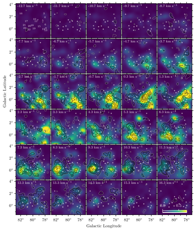
Figure 7: ¹³CO intensity, in units of K (see colorbar in Channel 16.3 km s^-1), at matched resolutions to C273$\alpha$. C273$\alpha$ contours, DR IDs, and “+” are the same as in Figure 3.

Channel maps of the MWISP ¹³CO emission (Su et al., 2019) with C273$\alpha$ contours overlaid are shown in Figure 7. Overall the C273$\alpha$ emission appears to coincide with the velocities where ¹³CO emission is present. However, their morphologies are noticeably different. C273$\alpha$ appears where ¹³CO is both relatively faint and bright. Peaks in emission are often spatially offset, and C273$\alpha$ is more often than not found on the outskirts of ¹³CO clouds. There are numerous examples of C273$\alpha$ spatially offset from ¹³CO ridges, for example at -2.7 km s^-1 below DR 15/12/13 and below DR 23, most of the emission in Channel 3.3 km s^-1 that forms a ridge, and in channel 1.3 km s^-1 just below DR 13 there is a distinct offset alongside CO emission.

There are also interesting regions where CRRLs are detected with strong significance but ¹³CO is comparatively fainter. This occurs generally in velocity channels of +10.3 km s^-1 and higher. C273$\alpha$ around DR 18/19/20/22 bridges two ¹³CO clouds in channel 0.3–1.3  km s^-1. C273$\alpha$ emission in channel -0.7 km s^-1 hugs the ¹³CO clouds below DR 22 and DR 23. Emission just above and to higher longitudes of DR 10 appears to “connect” two ¹³CO clouds starting at 6.3 km s^-1 and continuing to 13.3 km s^-1. The linear extent of C273$\alpha$ emission in Channel 7.3 km s^-1 is not matched in ¹³CO emission.

At this matched resolution, corresponding to about 21 pc, C273$\alpha$ shows considerably more structure than ¹³CO. This might arise from and possibly indicate the ubiquity of CO emission in this region at numerous scales, whereas for C273$\alpha$ emission may be less volume filling and/or thinner along some dimensions.

6.2 Flux Comparison

Figure 8 compares the emission in the C273$\alpha$ and ¹³CO data cubes. We show a voxel by voxel comparison of line brightness, for which we only plot voxels for which C273$\alpha$ is detected with $\geq 5\sigma$ significance, and we also show a comparison of the velocity-integrated emission of each 2D spatial pixel. The C273$\alpha$ emission has a factor of 3 difference from the faintest voxels ($\approx 7\times 10^{-4}$) to the brightest ($\approx 2\times 10^{-3}$). ¹³CO emission spans a factor closer to 10 in this range. There is a mildly increasing positive trend, as the intensity of ¹³CO increases so does C273$\alpha$. However, the brightest ¹³CO emission does not correspond to the brightest C273$\alpha$ values. C273$\alpha$ peak values of $10^{-3}$ coincide with the full range of ¹³CO values present.

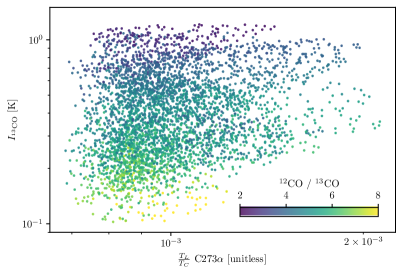
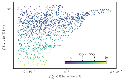
Figure 8: No clear correlation between the Top: Per voxel comparison of the ¹³CO intensity and the C273$\alpha$, where C273$\alpha$ is detected at $\geq 5\sigma$. Bottom: The velocity-integrated ¹³CO and C273$\alpha$ of each 2D spatial pixel.

It is a striking take away that C273$\alpha$ emission from cold dark gas is present over a large range of ¹³CO integrated intensity and in proportion, column density.

We looked for trends that might be present in the data. We investigated if the cloud velocity, latitude, longitude, distance from the center of the pointing (i.e., Cyg OB2) and we did not find an obvious indication of correspondence. Coloring the data points depending on the intensity ratio of ¹²CO/¹³CO indicates the optical depth effects of CO are at play. ¹²CO/¹³CO ratios are 3-10, in comparison to the optically thin ratio of 67 (Lucas & Liszt, 1998), indicating that ¹²CO is optically thick. The trend revealed by the CO intensity ratios indicates that optical depth effects might be causing more of a correlation that would otherwise be even further spread apart in this parameter space.

In the velocity-integrated comparison, there is also a regime in which C273$\alpha$ and ¹³CO do seem well correlated, in particular at integrated ¹³CO intensities of 7–9 K km s^-1. Using methods described in (Schneider et al., 2010), the ¹³CO flux of 7–9 K km s^-1 converted into a column density of H₂, assuming an excitation temperature of 10–20 K, implies $N(H_{2})=(3-5)\times 10^{21}$ cm^-2.

There seems to be two regimes, conditions where C273$\alpha$ and CO emission tightly relate to each other, and regions where C273$\alpha$ peaks independently of ¹³CO intensity. Cold CNM/dark envelopes around CO-bright clouds could gather enough material to trigger an intensity correlation between CO and C273$\alpha$. Whereas the second regime could relate to CO-dark, CNM-like clumps with a mix of H i and H₂, or pure dense H i.

Changes in the EUV and FUV intensities are also considerable throughout the region (e.g., Emig et al., 2022) and contribute to variations in local physical conditions (possibly for the two aforementioned regimes). Differing physical conditions further corroborates deviations in the C273$\alpha$ intensity from a tight relation, as the C273$\alpha$ emission can also changes by factors of a few depend on the physical conditions (see Section 4).

6.3 Spatial Separation of C273$\alpha$ and ¹³CO emission

We compare the angular separation of peaks in C273$\alpha$ and ¹³CO emission in each channel map. We identified emission peaks through dendrogram structures, making use of the Astrodendro (Rosolowsky et al., 2008) python package. Dendrograms locate islands of pixels with increasing-only intensities are identified around a local maximum in emission. For C273$\alpha$, we used a threshold of 5$\sigma$ and a minimum of three pixels to define peaks. For ¹³CO emission, we set the threshold of 0.1 K km s^-1 and a minimum of three pixels above the threshold.

For each peak of C273$\alpha$ emission, we located the ¹³CO peak in the same channel which was closest in angular separation. We plot the probability density function of these results in Figure 9, which was estimated using a Gaussian kernel and applying Scott’s Rule to determine the bin size. The distribution shows a peak at 26^′, corresponding to 12 pc. 26^′ is close to half the size of the beam (24^′), but it is much larger than the pointing accuracy of the observations (1^′). The distribution of angular separations between C273$\alpha$ and ¹³CO peaks quantifies the differences that can be seen by-eye in Figure 7.

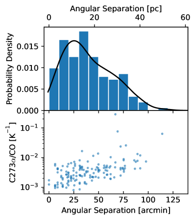
Figure 9: Top: Spatial separation between CRRL peaks and the closest ¹³CO peak identified in channel maps. A peak in the separation is found at 26^′ (12 pc), which is larger than the pointing accuracy of 1^′. Bottom: The angular separation plotted with the CRRL/¹³CO intensity ratio at the pixel of the CRRL peak. The intensity ratio of CRRL/¹³CO tends to be larger when the angular separation between intensity peaks is larger.

6.4 Comparisons with ¹³CO line profiles

With the high signal-to-noise nature of ¹³CO data, (unlike C273$\alpha$), we were able to use GaussPy+ to automate fitting the aperture spectra of Figure 5. Examples of the fitted components and residual spectra and a description of the fitting procedure in Appendix B. In total, 496 components were fit to the ¹³CO spectra.

6.4.1 Velocity Offsets

In Figure LABEL:fig:line_props we show the central velocities of all fitted ¹³CO components overlaid with C273$\alpha$ components. Curiously the central velocities of C273$\alpha$ and ¹³CO components appear to be somewhat anti-correlated, where the C273$\alpha$ emission appears at local deficits of ¹³CO. The typical error of the ¹³CO velocity centers is 0.2 km s^-1.

We also compare the difference in central velocities between ¹³CO and C273$\alpha$ components. For each fitted C273$\alpha$ component in an aperture, we identify the best-fit ¹³CO component that falls closest in velocity, defined as having the smallest absolute value of the velocity difference. We plot these results in Figure 10. The PDF is Gaussian-like. The standard deviation of the velocity differences, 2.9 km s^-1, is larger than the combined errors of the fitted centers, 0.53 km s^-1. This quantifies the velocity differences which can be seen by eye in the spectra and channel maps of the two tracers.

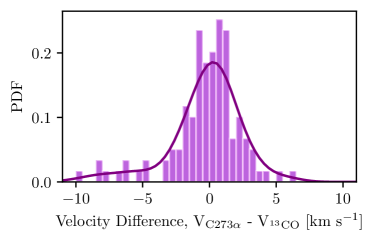
Figure 10: The velocity difference between each C273$\alpha$ component and the ¹²CO component nearest in velocity for a given aperture. The standard deviation of this distribution is 2.9 km s^-1.

Furthermore, the center of the $\mathrm{V_{C273\alpha}-V_{{}^{13}CO}}$ distribution, 0.2 km s^-1, is consistent with zero within the error. When we sub-select for different regions or velocity groupings in the map, the $\mathrm{V_{C273\alpha}-V_{{}^{13}CO}}$ distribution is consistently centered about zero within error. This implies that the flow of the C273$\alpha$ gas is not dominated by one systematic velocity, but rather a distribution of both red- and blue-shifted velocities.

Numerical studies and observations are finding that dynamical effects may be an important aspect to the molecular formation process, rapidly speeding up the timescales over which H i is converted into H₂ (Glover & Mac Low, 2007; Beuther et al., 2014; Valdivia et al., 2016; Gong et al., 2017; Bialy et al., 2017; Bisbas et al., 2017; Clark et al., 2019a; Heyer et al., 2022).

Park et al. (2023) found velocity differences between cold H i and CO of 0.4 km s^-1 towards an ensemble of local diffuse clouds, whereas velocity differences between warm H i and CO in their sample are 1.7 km s^-1. A smaller velocity difference in their diffuse clouds could be the result of different dynamics at play due to star formation and stellar feedback and/or the higher density environment that is found in Cygnus X.

Velocities of cold neutral gas in the range 1-4 km s^-1 are typically found for infalling under gravitational collapse on pc scales (Schneider et al., 2010; Beuther et al., 2015; Dhabal et al., 2018; Williams et al., 2018; Wang et al., 2020; Bonne et al., 2020; Heyer et al., 2022; Bonne et al., 2023). However, the scales probed by the C273$\alpha$ observations, a 48^′ beam equivalent to 21 pc, or consider the typical angular separation between ¹³CO and C273$\alpha$ of 12 pc (Section 6.3), larger velocities may be involved.

Conversely, with $10^{6}$ $\rm M_{\odot}$ in a region with a diameter of $\sim$100 pc, the escape velocity is $\sim$10 km s^-1. We do not (yet) see clear evidence for this kind of coherent velocities that could indicate that material is blown away before it can participate in star formation.

6.4.2 Line widths

Figure LABEL:fig:line_props also shows the distribution of line-widths of the fitted ¹³CO components with the C273$\alpha$ components. A median value of FWHM${}_{{}^{13}\mathrm{CO}}=2.5$ km s^-1 and error of 0.5 km s^-1 is found for ¹³CO. The C273$\alpha$ line width of FWHM${}_{\mathrm{C}273\alpha}=10.6$ km s^-1 is comparatively larger than that found for ¹³CO. The distribution of line widths is significantly more peaked for ¹³CO. While ¹³CO may consist of both dense filament like structure as well as fluffy diffuse components, it does not show a bimodal or broad distribution of line width. C273$\alpha$ appears to be dynamically more active and variant that ¹³CO.

The differences in the line width distributions could also be influenced by the C273$\alpha$ emission being weighted by density squared (i.e., $EM$), rather than density as for ¹²CO. Whereas a diffuse ¹³CO cloud component can dominate over narrow, dense filaments at larger scales, the same may not be the case for CRRL emission. This is supported by C273$\alpha$ showing more variation in emission structure, resulting in a less cloud-like and more ridge-like morphology.

The spread in the ¹³CO line width distribution is significantly smaller than for C273$\alpha$, and is well represented by its characteristic value. Mach numbers of 12–14 are derived in gas with temperatures of 15–20 K, consistent with $5<\mathcal{M}<20$ typically found within CO-emitting molecular clouds (Zuckerman & Palmer, 1974; Brunt, 2010). It is interesting that at least some of the C273$\alpha$ emission has similar Mach numbers as the ¹³CO material, which would be expected for gas tracing similar (i.e., H₂) states.

7 Discussion

7.1 Forming Molecular Gas at the DR21 filament

The DR21 and W75N regions in Cygnus X are iconic massive star-forming regions which have been extensively studied in the literature (Reipurth & Schneider, 2008). The dense filaments of molecular gas associated with each of these regions are undergoing gravitational collapse (Schneider et al., 2010; Li et al., 2023; Zeng et al., 2023). The DR21 and W75N clouds are colliding head-on (Dickel et al., 1978; Dobashi et al., 2019) and/or are forming from the interaction of composite H i and H₂ clouds (Schneider et al., 2023; Bonne et al., 2023). The slightly closer W75N cloud, at $1.3\pm 0.1$ kpc (Rygl et al., 2012), is moving away from the observer, with a red-shifted systemic velocity of $\sim$9 km s^-1. The slightly more distant DR21 cloud, at $1.5\pm 0.1$ kpc (Rygl et al., 2012), is moving towards the observer with a blue-shifted systemic velocity of $-$3 km s^-1 (see Figure 11). A molecular component centered at 3.5 km s^-1 could be emission bridging the clouds as a result of the collision (e.g., Haworth et al., 2015; Dobashi et al., 2019) and/or related to a foreground ($d\sim 600-800$ pc) cloud, the Cygnus Rift (e.g., Schneider et al., 2006).

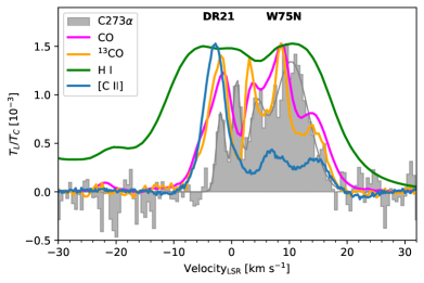
Figure 11: Spectra encompassing well-known DR 21 ($\sim-3$ km s^-1) and W75N ($\sim+9$ km s^-1) regions in Cyg X North, the region in our footprint for which spectrally-resolved [C ii] 158 $\mu$m data have been taken. Spectra of H i, ¹²CO, ¹³CO, and [C ii] have been normalized to the peak of C273$\alpha$.

A footprint covering DR21 and W75N is the only region in our C273$\alpha$ map for which [C ii] 158 $\mu$m emission has so far been observed at high spectral resolution, thanks to the SOFIA legacy program FEEDBACK (Schneider et al., 2020). Using the SOFIA FEEDBACK data, Schneider et al. (2023) investigated the low excitation [C ii] emission from W75N and a high velocity component ($v_{\mathrm{LSR}}=4-20$ km s^-1), and Bonne et al. (2023) investigated the low excitation [C ii] associated with DR21 at $v_{\mathrm{LSR}}\lesssim 0$ km s^-1.

The SOFIA FEEDBACK data covers a 0.26 deg² footprint centered about $(\ell,b)=(81.605^{\circ},+0.559^{\circ})$. In Figure 11, we plot the [C ii] spectrum averaged over the FEEDBACK footprint. We also overlay the C273$\alpha$, H i 21 cm, ¹²CO, and ¹³CO emission that has been extracted from a single pixel of 48^′ resolution data. Our beam size equates to an area of 0.45 deg² and is a bit larger than the [C ii] footprint.

Four Gaussian components fit to the C273$\alpha$ spectrum result in the lowest Bayesian and Akaike information criteria, in comparison to one, two, three, five, or six component fits. The properties of the best-fit profiles are given in Table 1 and plotted in Figure 11. These components are generally separated in velocity from CO components, by 2–3 km s^-1. They are all on the narrow end of the line-width distribution determined for our full survey data (Section 5), with the higher S/N in this location helping to discern narrower profiles.

Table 1: C273$\alpha$ Line Profiles of DR21/W75N (see Figure 11)

Vcen	Peak	FWHM
[km s-1]	[$T_{L}/T_{C}~10^{-3}$]	[km s-1]
-1.86 ±0.16	0.83 ±0.14	1.74 ±0.38
0.84 ±0.12	1.15 ±0.15	1.62 ±0.54
4.24 ±0.27	0.76 ±0.13	3.06 ±0.80
10.27 ±0.27	1.34 ±0.07	7.11 ±0.68

Note. — Best-fit Gaussian properties: “V_cen” is the central velocity, and “Peak” is the peak amplitude, and “$\sigma_{v}$” is the Gaussian width.

The C273$\alpha$ $-1.9$ km s^-1 component coincides with [C ii] emission from the cold H i and molecular subfilaments of DR21, falling predominately over -3 to -1 km s^-1 as characterized at high resolution (14^′′, 0.1 pc) by Bonne et al. (2023). In Figure 11, this low excitation [C ii]-emitting gas is confused by the bright [C ii] associated with the DR21 high density PDR ($v_{LSR}\sim-3$ km s^-1). At 0.1 pc resolution, the low-excitation [C ii] line widths were found to be 4.0–5.0 km s^-1; the [C ii] appears as a thin sheet of approximate density $n\approx 5000$ cm^-3, embedding molecular subfilaments that are about 0.3 pc in size (Hennemann et al., 2012) and have molecular line widths of $<1.3$ km s^-1. Even in the 48^′ GBT beam, the C273$\alpha$ line-widths are smaller than those of [C ii]. The C273$\alpha$ gas is therefore likely colder and denser than the [C ii] gas. The warmer gas which emits at 158 $\mu$m has larger turbulent and bulk motions, while the cooler gas emitting in the CRRL is considerably more quiescent. Either a $\sim$single coherent C273$\alpha$ component dominates even on large scales, or if Doppler broadening of multiple components is present at this scale, then the line widths of individual components are intrinsically smaller. In either case, C273$\alpha$ reasonably has a higher molecular gas fraction than [C ii]. Low-frequency CRRL emission towards Cas A was also found to have a high molecular gas fraction (Salas et al., 2018). With $\ell_{CO-dark}\approx 0.2\cdot\ell_{CO}$ (Wolfire et al., 2010), the pathlength of (a collection of) C273$\alpha$ layers could approach $\sim 0.1$ pc.

Bonne et al. (2023) performed a detailed comparison of the gravitational potential, magnetic field, and turbulent support in DR21, and determined that the gravitational energy dominates. The velocity offset of [C ii], 1–2 km s^-1, is attributed to gravitational collapse. Infalling molecular gas in the region has smaller velocity differences of $\sim$0.6 km s^-1 (Schneider et al., 2010). The velocity offset of C273$\alpha$ melds well into this picture.

Furthermore, we also reason that C273$\alpha$ emitting gas is inflowing onto the DR21 cloud. C273$\alpha$ is only observable when illuminated by background continuum emission. DR21 is more distant within the Cygnus X complex than W75N, and so the C273$\alpha$ emission we observe likely falls in regions of the cloud that are on the near side of the main DR21 cloud. Therefore, since the C273$\alpha$ emission is at comparable and only red-shifted velocities with respect to the DR21 cloud’s systemic velocity, the bulk motion of C273$\alpha$ would inflow towards the cloud. This indicates that C273$\alpha$ is tracing cold-dark material accreting onto the cloud.

Like DR21, the W75N cloud, at $8.6\pm 0.25$ km s^-1, is known to be experiencing gravitational collapse which dominates over magnetic support (Zeng et al., 2023). The brightest C273$\alpha$ component at 10.3 km s^-1 seems most likely to be associated with W75N. In Figure 11, a velocity offset between the C273$\alpha$ and ¹²CO of about 1.7 km s^-1 is present, red-shifted. Molecular gas within and connected to the W75N area is known to span a large velocity range, with brightest emission over a gradient of 8 to 11 km s^-1 (Dickel et al., 1978; Schneider et al., 2006). Schneider et al. (2023) also find low excitation [C ii] gas that spans 4–12 km s^-1.

7.2 Supernova Remnant G78.2+2.1 and the NGC 6910 cluster

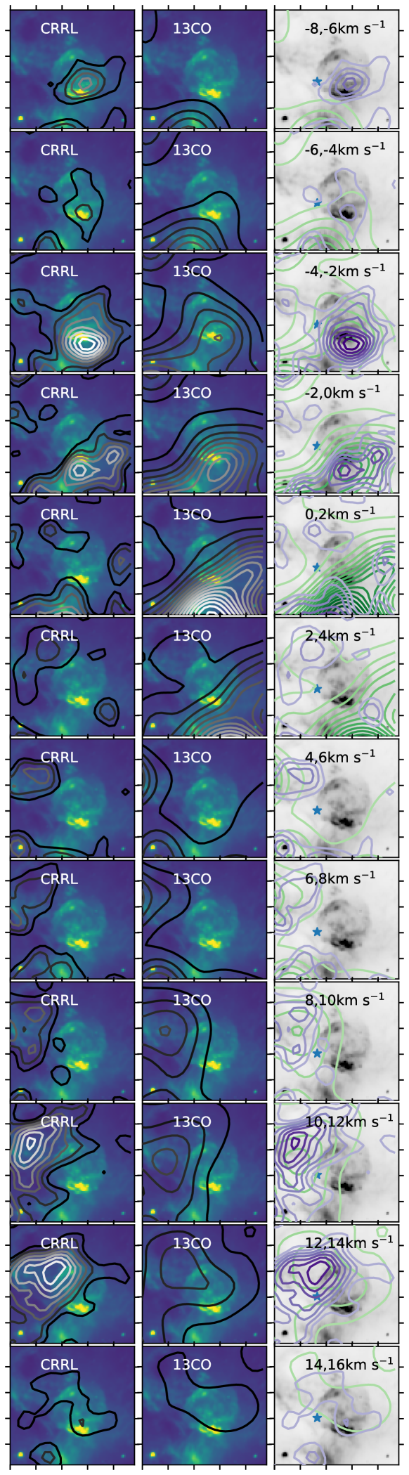
Figure 12: Emission in the region of the SNR $\gamma$-Cygni and cluster NGC 6910 (blue star). 1.4 GHz continuum emission is the background image. Maps integrated over 2 km s^-1 show C273$\alpha$ contours (left column), ¹³CO contours (middle column), and with both C273$\alpha$ (purple) and ¹³CO (green) contours overlaid (right column).

The shell-type supernova remnant (SNR) G78.2+2.1 has a distance of about 1.8 kpc (Higgs et al., 1977). It has been associated with the $\gamma$-Cygni nebula (Higgs et al., 1977), the radio continuum sources DR3 and DR4 (Downes & Rinehart, 1966), and with the pulsar PSR J2021+4026 (Trepl et al., 2010). H i absorption and emission features have been investigated for interaction and influence with the SNR (Landecker et al., 1980; Braun & Strom, 1986; Gosachinskij, 2001; Ladouceur & Pineault, 2008; Leahy et al., 2013). H i absorption against the SNR continuum is detected at least at the LSR velocities of -8 km s^-1 to +20 km s^-1, also the approximate range covered by the molecular gas in the region. It is clear that the SNR is at a distance further than the material associated with these velocities, but discerning which components possibly associate with the SNR interaction remains challenging, leading to multiple scenarios proposed (e.g., Ladouceur & Pineault, 2008).

C273$\alpha$ is observed from about -8 to 16 km s^-1 in a 2.5^∘ $\times$ 2.5^∘ region in this direction (Figure 12). Roshi et al. (2022) observed DR4 at 321 and 800 MHz with the GBT, and characterized a single velocity component in this direction ($v_{\mathrm{LSR}}=-2.7\pm 0.3$ km s^-1), albeit with 4 km s^-1 channel resolution. They noted the CRRL central velocity coincides with the velocity of an H i self-absorption component in CGPS data.

With the mapped area and at high spectral resolution, we find additional components and image their kinematics. The kinematics of the blue-shifted C273$\alpha$ emission, see Figure 12, are consistent with an expanding shell moving at (at least) $\sim$8–10 km s^-1, with observed central velocities of -9 km s^-1 up to, possibly, +1 km s^-1. Comparable scenarios, including some with larger expansion velocities, have been proposed (Landecker et al., 1980; Ladouceur & Pineault, 2008; Leahy et al., 2013). C273$\alpha$ emission appears as unique spatio-spectral peaks, at -7 km s^-1 and -3 km s^-1. These may be two condensations of molecular gas. The spectral profiles show the asymmetry expected of an expanding shell of material, with lower level emission at the most extreme velocities peaking closest to the projected center of the supernova remnant shell and with the brightest emission closest to the shell edges in projection. The C273$\alpha$ component at -8 to -6  km s^-1 is coincident with the most blue-shifted components of H i absorption at $\sim$-8 km s^-1 (Leahy et al., 2013).

The morphology of the emission at -1 km s^-1 is elongated at the Southern rim of the supernova remnant. And in the 1 km s^-1 channel, three regions surrounding the shell also appear in C273$\alpha$ emission. However, emission at -1 km s^-1 to 3 km s^-1 shows morphologies possibly related to the massive star cluster NGC 6913, as described in Section 7.3. In any case, it is interesting to note there are C273$\alpha$ emission peaks which surround ¹³CO emission peaks in the -1 km s^-1 channel.

The red-shifted C273$\alpha$ emission must be in front of the supernova remnant, otherwise the C273$\alpha$ strength (as a line-to-continuum ratio) would be significantly diluted by the strong continuum of the supernova remnant. Therefore the redshifted C273$\alpha$ components should not be related to the receding side of an expanding shell, at odds with the scenarios that suggest this association (Ladouceur & Pineault, 2008). The redshifted C273$\alpha$ emission extends to about 15 km s^-1, velocities that Landecker et al. (1980) suggested harbor a cold H i screen. The cloud dynamics in this portion of the Cygnus X region may be projected onto but fully unrelated to the SNR.

C273$\alpha$ and ¹³CO emission start to appear in the NE of Figure 12 from about 5 km s^-1 and up. In channels 7-9 km s^-1, C273$\alpha$ appears as two local peaks again surrounding a ¹³CO peak. In channel 11 km s^-1 C273$\alpha$ forms an arc like structure, and maintains brightness in the 13 km s^-1 channel. The massive star-cluster NGC 6910, at a distance of $1.7\pm 0.1$ kpc (Cantat-Gaudin & Anders, 2020; Quintana & Wright, 2022) may have some influence. It has a stellar mass of $10^{3}$ $\rm M_{\odot}$ (Le Duigou & Knodlseder, 2002) and age of $6\pm 2$ Myrs (Kolaczkowski et al., 2004). The arc in the 13 km s^-1 channel may very well be related to photoionizing and/or stellar-wind feedback from the $\sim$30 OB stars making up NGC 6910 (Le Duigou & Knodlseder, 2002).

7.3 The massive star-cluster NGC 6913

The PDR that extends in Figure 1 along DR4 and DR5 down to DR13 may be the PDR rim of a bubble powered by the massive star-cluster NGC 6913 (Schneider et al., 2007). NGC 6913 (M29) hosts about 20 OB stars (Le Duigou & Knodlseder, 2002). C273$\alpha$ emission extending at negative velocities could relate to the rim of that stellar bubble. We show a C273$\alpha$ emission integrated over -4 to 2 km s^-1 in Figure 13. Compressed, cooling gas behind the PDR rim could be rich in cold H i and/or CO-dark H₂.

Figure 13: PAH emission at 8.3 $\mu$m with C273$\alpha$ integrated from -4 to 2 km s^-1 overlaid, showing what a bubble powered by the cluster NGC 6913.

7.4 Size Scales of Cold Dark Gas from C273$\alpha$

Cold dark gas in our Galaxy is distributed anisotropically (Heiles & Troland, 2003, 2005). Cold H i in emission (Clark et al., 2014) and absorption (McClure-Griffiths et al., 2006) reveal ubiquitous filamentarity. These narrow ($\sim$0.1 pc) (Clark et al., 2014; Kalberla et al., 2016) density structures (Clark et al., 2019b) have high aspect ratios ($\gtrsim 100$; Kalberla & Haud, 2023). Their orientation appears to be parallel to magnetic fields at column densities of $N(H)<5\times 10^{21}$ cm^-2 and perpendicular at higher column densities (McClure-Griffiths et al., 2006; Clark et al., 2015; Planck Collaboration et al., 2016; Kalberla et al., 2020). While these structures are characterized by the presence of H i, they may also contain predominantly molecular gas (Kalberla et al., 2020). Strasser et al. (2007) estimate that the mean distance between cold absorbing clouds is 90–220 pc.

Low-frequency CRRLs have been directly connected to HISA from cold dark filaments in the Sun’s local bubble (Roshi & Kantharia, 2011). Roshi & Kantharia (2011) estimated line-of-sight CRRL path lengths in the range 0.03–3.5 pc in the Riegel-Crutcher Cloud at a spatial resolution of $4.4\times 1.3$ pc² (2^∘ $\times$ 0.6^∘). These are in excellent agreement with tracing CNM filaments in swept up shells. Towards another line-of-sight, the supernova remnant Cassiopeia A, CRRLs associate with a large molecular cloud in the Perseus spiral arm. CRRL analyses of two bright gas components with LOFAR and WSRT have determined path lengths of the CRRL-emitting gas with small uncertainty. Oonk et al. (2017) determined a path length of $35.3\pm 1.2$ pc for the gas across the 6^′ (5.5 pc) extent of Cas A. Salas et al. (2018) resolved this region at 70^′′ (1.0 pc) to directly show the CRRLs tracing the surface of the CO-cloud, with projected spatial separations between ¹²CO and CRRL emission of 1–2 pc. Their line-of-sight integrated path lengths varied between 27–182 pc for a single velocity component. Chowdhury & Chengalur (2019) used GMRT 430 MHz observations at 18^′′ (0.3 pc) resolution which show point-like condensations and linear-like bright emission that have unresolved widths ($<0.3$ pc) and a linear extent of $>3$ pc. The single velocity component indicates a coherent gas structure, but the long path lengths indicate sheet-like CNM structure, which contrasts with filament structure as determined from H i and dust emission analyses.

Cygnus X is a site of vigorous star formation with a massive molecular cloud complex and thus different from the local H i cloud structures and the “random” sight-lines probed by the observations discussed above. In Cygnus X, we see a new window into cold dark gas structure as probed by low-frequency CRRLs, in a region where more than 170 OB stars are actively churning up their molecular cloud environment, blowing bubbles, illuminating, photo-evaporating, and photo-ionizing molecular cloud edges, and pushing gas around onto and away from clouds. The C273$\alpha$ emission provides a window into these feedback activities.

The C273$\alpha$ morphology indeed shows filamentarity of cold dark gas, similar to previous works. This filamentarity spans more than 100 pc and contains numerous spatio-spectral coherent structures. Not only filamentarity, but a mixture of point-like condensations ($\sim$10 pc) and extended sheet-like structures appear on these scales. The mean separation inferred between these “clouds” is thus considerably smaller, while their coherent extent is larger than previous works (Strasser et al., 2007; Bellomi et al., 2020). It could be that some of the structures are exposed cloud cores or long, thin illuminated cloud edges (e.g., Emig et al., 2022).

7.5 Estimated C273$\alpha$ gas densities

Steady-state analytical models have been constructed and widely applied to describe the H i-to-H₂ transition in the ISM of galaxies (e.g., Krumholz et al., 2008, 2009; McKee & Krumholz, 2010; Wolfire et al., 2010; Sternberg et al., 2014; Gong et al., 2017). The Wolfire et al. (2010) models predict sizes for the total cloud including H i ($R_{\mathrm{T}}$), with respect to the CO radius of the cloud ($R_{\mathrm{CO}}$) and an H₂ CO-dark radius of the cloud ($R_{\mathrm{H}_{2}}$). The nominal values expected for the ratios are $R_{\mathrm{H}_{2}}/R_{\mathrm{CO}}\approx 1.2$ and $R_{\mathrm{T}}/R_{\mathrm{CO}}\approx 1.3-1.4$.

We use the Wolfire et al. (2010) size relation together with the angular separation between C273$\alpha$ and ¹³CO (Section 6.3) to approximate gas density. Photo-dissociation region (PDR) models suggest low-frequency CRRLs arise from $A_{V}\approx 0.3-1$ depending on local conditions (e.g., Salas et al., 2018), corresponding to column densities of $N(H)=(0.6-1.9)\times 10^{21}$ cm^-2 when using the relation $N(H)=A_{V}\cdot 1.9\times 10^{21}$ cm^-2. If we assume the CO-dark H2 layer is given by $R_{H_{2}}=12$ pc, then we derive densities of $n_{H}=N(H)/(\Delta R_{H2})=(100-300)$ cm^-3. The width of the CO-dark H2 layer is assumed to be $\Delta R_{H2}=R_{H2}-R_{CO}=R_{H2}-(1/1.2)R_{H2}=0.17R_{H2}=2.0$ pc.

If we assume 12 pc indicates where an atomic layer of the cloud is, slightly higher cloud densities are called for, $n_{H}\approx(120-370)$ cm^-3, for which $\Delta R_{HI}=0.14R_{HI}=1.7$ pc. The spatial distribution peaks at 12 pc, but has tail extending to 30 pc and beyond. An $R_{H2}=30$ pc, would imply densities in the range $n_{H}\approx 40-120$ cm^-3.

The C273$\alpha$ emission arises from cold relatively diffuse gas with hydrogen densities of $n_{H}\approx 40-400$ cm^-3, or equivalently, electron densities of $n_{e}\approx 0.006-0.06$ cm^-3 assuming a carbon abundance of $A_{c}=1.4\times 10^{-4}$ (Sofia et al., 2004).

7.6 Pressure estimates of the cold dark gas

We estimate and compare pressure terms in order to understand what dominates the dynamics and evolution of the cold dark gas. On these scales, we find that the turbulent pressure likely dominates. The turbulent pressure is given by $P_{\mathrm{turb}}=\rho V_{\mathrm{rms}}^{2}$ where $\rho$ is the mass density and the rms velocity dispersion, $V_{\mathrm{rms}}$ is related to the line-of-sight velocity dispersion as $V_{\mathrm{rms}}=\sqrt{3}\sigma_{v}$. For a nominal electron density of the C273$\alpha$ gas of $n_{e}\sim 0.03$ cm^-3 ($n_{H}\sim 200$ cm^-3), the mass density is estimated as $\rho_{\mathrm{HI}}\approx 1.36m_{\mathrm{H}}(n_{e}/A_{c})$ and/or $\rho_{\mathrm{H_{2}}}\approx 2.36m_{\mathrm{H}}(n_{e}/A_{c})$. With $A_{c}=1.4\times 10^{-4}$ (Sofia et al., 2004) and $V_{\mathrm{rms}}=7.8$ km s^-1, the turbulent pressure is $P_{\mathrm{turb}}/k_{B}\approx(\frac{n_{e}}{0.03~\mathrm{cm^{-3}}})2.1-3.6\times 10^{6}$ cm^-3 K.

The thermal pressure of the CRRL gas is small, where $P_{\mathrm{therm}}=k_{B}(n_{e}/A_{c})T_{e}$. For gas with $n_{e}=0.03$ cm^-3 and $T_{e}=50$ K, the thermal pressure is $P_{\mathrm{therm}}/k_{B}\approx(\frac{n_{e}}{0.03~\mathrm{cm^{-3}}})1\times 10^{4}$ cm^-3 K. In comparison, the ram pressure imparted by the C273$\alpha$ emitting gas is given by $P_{\mathrm{ram}}=\rho V^{2}$ where $\rho$ is the mass density and $V$ is the velocity. Assuming a nominal electron number density $n_{e}\sim 0.03$ cm^-3 and velocity of $V=2.9$ km s^-1, the estimated ram pressure is $P_{\mathrm{ram}}/k_{B}\approx(\frac{n_{e}}{0.03~\mathrm{cm^{-3}}})(3.0-5.1)\times 10^{5}$ cm^-3 K.

Emig et al. (2022) investigated diffuse ionized gas structures throughout Cygnus X and estimated its thermal pressure to typically be $P_{\mathrm{ion}}/k_{B}\approx 6\times 10^{5}$ cm^-3 K, which was also in agreement with the X-ray studies $P_{X}/k_{B}\approx 6\times 10^{5}$ cm^-3 K. Much higher pressures are associated with compact HII regions such as DR21. The magnetic pressure is on the order of $P_{\mathrm{mag}}/k_{B}\approx 2\times 10^{5}$ cm^-3 K, assuming the magnetic field strength of $B=0.1$ mG in the ambient ISM near DR21 (Ching et al., 2022).

Higher turbulent pressures than magnetic pressures were also found with the CRRL observations towards Cas A (Oonk et al., 2017).

We estimate the eddy turnover time of a turbulent medium, $t_{\mathrm{turb}}=L/(V_{\mathrm{rms}})$, for the given size scales and line widths that we derive for the C273$\alpha$-emitting gas. Taking $L=21$ pc, equivalent to the beam size, and $V_{\mathrm{rms}}=7.8$ km s^-1 as above, the eddy turnover time is 2.6 Myr. In turbulent ISM models of molecular cloud formation, this sets an upper limit for the timescale of H₂ formation, which does not depend on the nature of the turbulence present (e.g., Micic et al., 2012). With an H₂ formation timescale that is dependent upon density as $t_{H_{2}}\approx(10^{3}\,\mathrm{Myr})/(n_{\mathrm{H}}\,\mathrm{[cm^{-3}]})$ (Hollenbach et al., 1971), 2.6 Myr estimate implies the density in the gas forming H₂ is $n_{\mathrm{H}}\sim 380$ cm^-3, or $n_{e}\sim 0.05$ cm^-3. The density we have roughly estimated by way of the line widths is quite comparable to the density estimated in Section 7.5 from the typically spatial separation of C273$\alpha$ and ¹³CO.

Could the velocity difference of ¹³CO with the C273$\alpha$ components (Section 6.4.1) represent free-fall velocities from gravitational collapsing material throughout the region? Combining the 2.9 km s^-1 velocity flow with the average spatial separation of 12 pc (Section 6.3), the timescale for the convergence of C273$\alpha$ material onto the molecular cloud is $t\sim 4$ Myr. This sits above the turbulent timescale of 2.6 Myr. Turbulence may appreciably act on the gas and form H₂ on spatial and time scales shorter than the build-up from the flow of material onto the cloud.

8 Conclusions

We surveyed carbon radio recombination lines (CRRLs) at 292–394 MHz with GBT over a $5.5^{\circ}\,\times\,5.5^{\circ}$ area in the Cygnus X ($d\sim 1.5$ kpc) star-forming region. The low-frequency CRRL emission is predominantly stimulated and originates in cold ($T\lesssim 100$ K) gas where carbon is singly ionized. We use these observations to investigate the H i-to-H₂ transition. This article presents the first large-scale mapping ($>$0.014 deg²; e.g., Salas et al., 2018) of low-frequency CRRLs from cold dark gas.

By stacking up to 28 CRRLs, we created a line-synthesized data cube with an effective transition of C273$\alpha$ at an effective frequency of 321.6 MHz and spatial resolution of 48^′ (21 pc). We characterized the spatial distributions and spectral line profiles of C273$\alpha$ and compared the properties with those of ¹³CO emission at matched resolutions. A summary of our results are as follows:

1. We detect C273$\alpha$ emission in the Moment 0 map with a significance greater than 3$\sigma$ over 24 deg² (75%) of the mapped region (Figure 1). The C273$\alpha$ emission spans LSRK velocities of -15 km s^-1 to 20 km s^-1, similar to ¹³CO (Figure 2), similar to ¹³CO.

2. The morphology of the C273$\alpha$ is complex and varied. Arcs, linear-like ridges, and bright point-like condensations are visible throughout the region. Emission in a velocity channel (Figure 3) is typically extended and possibly sheet-like, and a given location typically has multiple velocity components present. Size scales emission range from 10 pc (24^′) to more than 100 pc. Some C273$\alpha$ bubbles and arcs may be related to the interaction of the SNR $\gamma$-Cygni with the surrounding ISM and stellar feedback bubbles surrounding the massive clusters NGC 6910 and NGC 6913.

3. To first order, locations with C273$\alpha$ emission are generally bright in ¹³CO. The tracers can have similar morphologies (Figure 7), with C273$\alpha$ sitting at the edges of peaked ¹²CO emission. In other instances, C273$\alpha$ emission appears where ¹³CO is relatively faint. At matched resolution, the C273$\alpha$ shows more structure, possibly indicating that it is not as wide-spread or volume-filling on all scales of ¹³CO emission.

4. The C273$\alpha$ spectral profiles are well fit by Gaussians, indicating they are not collision or radiation broadened. They are likely to be turbulently broadened. The median FWHM_C273α is $10.6$ km s^-1, but the line widths range from 2 – 20 km s^-1. In comparison, the median line width fitted for ¹³CO is FWHM${}_{\mathrm{{}^{13}CO}}=2.5$ km s^-1. The characteristic C273$\alpha$ line width implies Mach numbers of $\mathcal{M}_{\mathrm{C}273\alpha}\approx 10-30$ for $T\approx 20-100$ K which is significantly higher than found towards diffuse ISM sight lines. The C273$\alpha$ line widths imply this gas is dynamically more active than the ¹³CO gas.

5. Velocity offsets between C273$\alpha$ and ¹³CO are apparent throughout the region. We compared the central velocity of each C273$\alpha$ fitted component with the ¹²CO component closest in velocity (within the same spatial aperture). The velocity difference, $V_{\mathrm{C}273\alpha}-V_{\mathrm{{}^{12}CO}}$, has a standard deviation of 2.9 km s^-1. In the DR21 / W75N region, the orientation and kinematics require C273$\alpha$ to be infalling towards the ¹³CO-traced gas.

6. Comparing the C273$\alpha$ and ¹³CO velocity-integrated pixel by pixel (Figure 8, two regimes emerge. In one regime, the two tracers are strongly related, at column densities $N(H)\approx(3-5)\times 10^{21}$ cm^-2. In the second regime, C273$\alpha$ emits independently of the ¹³CO intensity. This points to regimes in which the envelopes of clouds (filaments) trigger a correlation, and cold clumps in a more-diffuse mix of H i and H₂ gas do not.

7. We characterize the angular separation between peaks of C273$\alpha$ emission and the closest peak of ¹³CO emission in channel maps. The angular separation reveals a characteristic separation of 12 pc and a tail out to 30 pc. C273$\alpha$ gas densities of $n_{H}\approx 40-400$ cm^-3 are implied by the separations with the Wolfire et al. (2010) models.

The C273$\alpha$ emission likely arises from C⁺/H₂ gas, commonly referred to as CO-dark molecular gas. On these scales, the evolution of the C273$\alpha$ gas is dominated by turbulent pressure, and it has a characteristic timescale to form H₂ of about 2.6 Myr.

Additional observations of low-frequency CRRLs in multiple radio bands will place constraints on the density and temperature of this gas component. These observations are a pilot survey to the GBT Diffuse Ionized Gas at Low Frequencies (GDIGS-Low; PI: P. Salas). GDIGS-Low is an extension to the GDIGS survey of RRLs at 5.8 GHz (Anderson et al., 2021). GDIGS-Low is mapping the Inner Galaxy with RRLs at the 340 and 800 MHz windows. Large systematic studies with GDIGS-Low and forthcoming observations with next-generation low-frequency telescopes will bring profound insights into cold dark gas using ionized carbon lines at low-frequencies. These observations highlight the GBT and the 340 MHz window (e.g., see also, Anantharamaiah, 1985; Roshi & Anantharamaiah, 1997; Roshi et al., 2002) as an excellent probe for CRRL studies.

Appendix A Noise Estimation

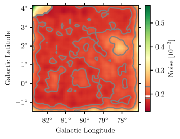
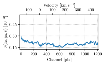
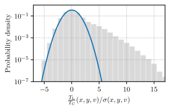
Figure 14: The top and middle panels show the noise along the spatial (top) and spectral (middle) coordinates. Gray contours in the top panel show the 50th and 90th percentiles of the noise values and the mean, $1.91\times 10^{-4}$, is indicated by a white line in the colorbar. The noise profile along the spectral axis (middle panel) is extracted from the center of the map. The bottom panel shows the probability density function of the signal-to-noise within the cube. The blue parabola shows the PDF of a normal distribution with mean of zero and variance of one. A normal distribution is an excellent description of the signal-to-noise values, except for the strong positive tail of values arising from signal in the cube.

We produce a three-dimensional estimate of the rms noise. Our methodology closely follows that of Leroy et al. (2021, see their Section 7.2). We first construct a noise map that captures spatial variations of the noise, $R(x,y)$. Then, we measure a normalized noise spectrum that captures relative spectral variations, $s(v)$. The noise in the data cube is then

$$\sigma(x,y,v)=R(x,y)s(v).$$ (A1)

We determine $R(x,y)$ and $s(v)$ empirically, determining the values from the data themselves using an iterative procedure. First, we compute spatial variations. We use the line-free channels 800–1200 (see Fig. 14) and calculate the standard deviation at each pixel, yielding an estimate of $R(x,y)$. Next, we compute spectral variations. We take all spatial pixels of a given channel. Then we exclude positive data that have high significance with respect to the noise level. These are likely to be associated with real emission and not noise. We do not exclude high-significance negative data. We then calculate the standard deviation for each channel while weighting each pixel with its spatial response $R(x,y)$. We normalize the noise standard deviation of each channel by the mean value. We then smooth these estimates with a third-order Savitsky–Golay filter to estimate $s(v)$.

The calculation of $R(x,y)$ is then repeated, but this time weighting each of the line-free channels by the estimate of $s(v)$. Then we repeat the calculation for $s(v)$. Finally, we iterate once more on the procedure to ensure convergence, and multiply the final $R(x,y)$ and $s(v)$ responses to generate an estimate of $\sigma(x,y,v)$. The iterative process drives the signal-to-noise distribution, $\frac{T_{\mathrm{L}}}{T_{\mathrm{C}}}(x,y,v)/\sigma(x,y,v)$, in the signal-free regions to a normal distribution centered on zero with a standard deviation of 1.

Figure 14 shows the empirically derived noise and the signal-to-noise distribution. The weighted mean of the noise is $\sigma_{T_{L}/T_{C}}=1.9\times 10^{-4}$ in 0.5 km s^-1 channels.

Appendix B Line fits

B.1 C273$\alpha$ Spectra

We show the Gaussian profiles fit to the C273$\alpha$ spectrum in each aperture region in Figure 15. The residual spectrum with the fit subtracted from the data is also plotted.

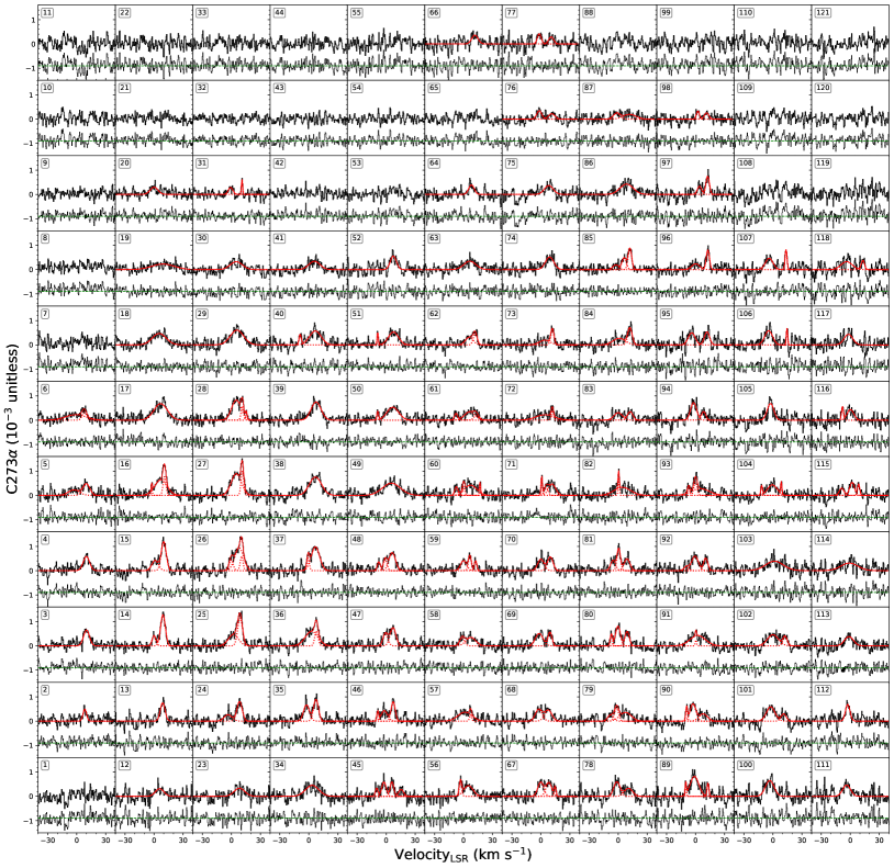
Figure 15: Fits to C273$\alpha$ emission.

B.2 ¹³CO Spectra

¹³CO spectra are presented in Figure 5. We used GaussPy+ to fit and decompose the ¹³CO line emission. Examples of the Gaussian profiles fit to the ¹²CO spectrum and the residuals of the spectrum with fits subtracted are shown in Figure 16.

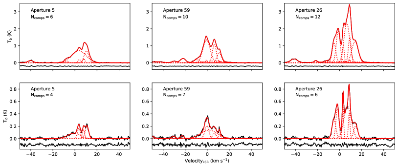
Figure 16: Top row is ¹²CO spectra and the bottom row is the ¹³CO spectra for the corresponding aperture regions. The aperture ID and the number of Gaussian components fit to the spectra are listed in the top right corner of each plot.

References

- Abeysekara et al. (2021) Abeysekara, A. U., Albert, A., Alfaro, R., et al. 2021, NatAs, 5, 465, doi: 10.1038/s41550-021-01318-y
- Ackermann et al. (2011) Ackermann, M., Ajello, M., Allafort, A., et al. 2011, Sci, 334, 1103, doi: 10.1126/science.1210311
- Anantharamaiah (1985) Anantharamaiah, K. R. 1985, JApA, 6, 177. https://ui.adsabs.harvard.edu/abs/1985JApA....6..177A/abstract
- Anderson et al. (2021) Anderson, L. D., Luisi, M., Liu, B., et al. 2021, ApJS, 254, 28, doi: 10.3847/1538-4365/abef65
- Beerer et al. (2010) Beerer, I. M., Koenig, X. P., Hora, J. L., et al. 2010, AJ, 720, 679, doi: 10.1088/0004-637X/720/1/679
- Bellomi et al. (2020) Bellomi, E., Godard, B., Hennebelle, P., et al. 2020, A&A, 643, A36, doi: 10.1051/0004-6361/202038593
- Berlanas et al. (2018) Berlanas, S. R., Herrero, A., Comerón, F., et al. 2018, A&A, 612, 50, doi: 10.1051/0004-6361/201731856
- Berlanas et al. (2019) Berlanas, S. R., Wright, N. J., Herrero, A., Drew, J. E., & Lennon, D. J. 2019, MNRAS, 484, 1838, doi: 10.1093/mnras/stz117
- Berlanas et al. (2020) Berlanas, S. R., Herrero, A., Comerón, F., et al. 2020, A&A, 642, 168. https://ui.adsabs.harvard.edu/abs/2020A%26A...642A.168B/abstract
- Beuther et al. (2015) Beuther, H., Ragan, S. E., Johnston, K., et al. 2015, A&A, 584, A67, doi: 10.1051/0004-6361/201527108
- Beuther et al. (2014) Beuther, H., Ragan, S. E., Ossenkopf, V., et al. 2014, A&A, 571, A53, doi: 10.1051/0004-6361/201424757
- Bialy et al. (2017) Bialy, S., Burkhart, B., & Sternberg, A. 2017, ApJ, 843, 92, doi: 10.3847/1538-4357/aa7854
- Bisbas et al. (2017) Bisbas, T. G., Tanaka, K. E. I., Tan, J. C., Wu, B., & Nakamura, F. 2017, ApJ, 850, 23, doi: 10.3847/1538-4357/aa94c5
- Bolatto et al. (2013) Bolatto, A. D., Wolfire, M., & Leroy, A. K. 2013, ARA&A, 51, 207, doi: 10.1146/annurev-astro-082812-140944
- Bonne et al. (2020) Bonne, L., Bontemps, S., Schneider, N., et al. 2020, A&A, 644, A27, doi: 10.1051/0004-6361/202038281
- Bonne et al. (2023) —. 2023, ApJ, 951, 39, doi: 10.3847/1538-4357/acd536
- Bontemps et al. (2010) Bontemps, S., Motte, F., Csengeri, T., & Schneider, N. 2010, A&A, 524, A18, doi: 10.1051/0004-6361/200913286
- Braun & Strom (1986) Braun, R., & Strom, R. G. 1986, A&A, 164, 193. https://ui.adsabs.harvard.edu/abs/1986A&A...164..193B
- Brocklehurst & Seaton (1972) Brocklehurst, M., & Seaton, M. J. 1972, MNRAS, 157, 179
- Brunt (2010) Brunt, C. M. 2010, A&A, 513, A67, doi: 10.1051/0004-6361/200913506
- Busch et al. (2019) Busch, M. P., Allen, R. J., Engelke, P. D., et al. 2019, ApJ, 883, 158, doi: 10.3847/1538-4357/ab3a4b
- Busch et al. (2021) Busch, M. P., Engelke, P. D., Allen, R. J., & Hogg, D. E. 2021, ApJ, 914, 72, doi: 10.3847/1538-4357/abf832
- Cantat-Gaudin & Anders (2020) Cantat-Gaudin, T., & Anders, F. 2020, A&A, 633, A99, doi: 10.1051/0004-6361/201936691
- Chevance et al. (2023) Chevance, M., Krumholz, M. R., McLeod, A. F., et al. 2023, in ASPC, Vol. 534, Kyoto, Japan, 1, doi: 10.48550/arXiv.2203.09570
- Ching et al. (2022) Ching, T.-C., Qiu, K., Li, D., et al. 2022, ApJ, 941, 122, doi: 10.3847/1538-4357/ac9dfb
- Chowdhury & Chengalur (2019) Chowdhury, A., & Chengalur, J. N. 2019, MNRAS, 486, 42, doi: 10.1093/mnras/stz779
- Clark et al. (2019a) Clark, P. C., Glover, S. C. O., Ragan, S. E., & Duarte-Cabral, A. 2019a, MNRAS, 486, 4622, doi: 10.1093/mnras/stz1119
- Clark et al. (2015) Clark, S. E., Hill, J. C., Peek, J. E. G., Putman, M. E., & Babler, B. L. 2015, PhRvL, 115, 241302, doi: 10.1103/PhysRevLett.115.241302
- Clark et al. (2019b) Clark, S. E., Peek, J. E. G., & Miville-Deschênes, M. A. 2019b, ApJ, 874, 171, doi: 10.3847/1538-4357/ab0b3b
- Clark et al. (2014) Clark, S. E., Peek, J. E. G., & Putman, M. E. 2014, ApJ, 789, 82, doi: 10.1088/0004-637X/789/1/82
- Comerón et al. (2020) Comerón, F., Djupvik, A. A., Schneider, N., & Pasquali, A. 2020, A&A, 644, 62. http://arxiv.org/abs/2009.12779
- Comerón & Pasquali (2012) Comerón, F., & Pasquali, A. 2012, A&A, 543, 1, doi: 10.1051/0004-6361/201219022
- Comrie et al. (2021) Comrie, A., Wang, K.-S., Hsu, S.-C., et al. 2021, zndo, doi: 10.5281/zenodo.3377984
- Dame et al. (2001) Dame, T. M., Hartmann, D., & Thaddeus, P. 2001, ApJ, 547, 792, doi: 10.1086/318388
- Deb et al. (2018) Deb, S., Kothes, R., & Rosolowsky, E. 2018, MNRAS, 481, 1862, doi: 10.1093/mnras/sty2389
- Dhabal et al. (2018) Dhabal, A., Mundy, L. G., Rizzo, M. J., Storm, S., & Teuben, P. 2018, ApJ, 853, 169, doi: 10.3847/1538-4357/aaa76b
- Dickel et al. (1978) Dickel, J. R., Dickel, H. R., & Wilson, W. J. 1978, ApJ, 223, 840, doi: 10.1086/156317
- Dobashi et al. (2019) Dobashi, K., Shimoikura, T., Katakura, S., Nakamura, F., & Shimajiri, Y. 2019, PASJ, 71, S12, doi: 10.1093/pasj/psz041
- Dobbs et al. (2014) Dobbs, C. L., Krumholz, M. R., Ballesteros-Paredes, J., et al. 2014, in Protostars and Planets VI, 3–26, doi: 10.2458/azu_uapress_9780816531240-ch001
- Downes & Rinehart (1966) Downes, D., & Rinehart, R. 1966, ApJ, 144, 937. https://ui.adsabs.harvard.edu/abs/1966ApJ...144..937D/abstract
- Emig et al. (2022) Emig, K. L., White, G. J., Salas, P., et al. 2022, A&A, 664, 88, doi: 10.1051/0004-6361/202142596
- Erickson et al. (1995) Erickson, W. C., McConnell, D., & Anantharamaiah, K. R. 1995, ApJ, 454, 125, doi: 10.1086/176471
- Glover & Mac Low (2007) Glover, S. C. O., & Mac Low, M.-M. 2007, ApJ, 659, 1317, doi: 10.1086/512227
- Gong et al. (2017) Gong, M., Ostriker, E. C., & Wolfire, M. G. 2017, ApJ, 843, 38, doi: 10.3847/1538-4357/aa7561
- Gosachinskij (2001) Gosachinskij, I. V. 2001, AstL, 27, 233, doi: 10.1134/1.1358380
- Grenier et al. (2005) Grenier, I. A., Casandjian, J.-M., & Terrier, R. 2005, Science, 307, 1292, doi: 10.1126/science.1106924
- Habing (1968) Habing, H. J. 1968, BAN, 19, 421. https://ui.adsabs.harvard.edu/abs/1968BAN....19..421H
- Hacar et al. (2023) Hacar, A., Clark, S. E., Heitsch, F., et al. 2023, in ASPC, Vol. 534, 153, doi: 10.48550/arXiv.2203.09562
- Harris et al. (2020) Harris, C. R., Millman, K. J., van der Walt, S. J., et al. 2020, Natur, 585, 357, doi: 10.1038/s41586-020-2649-2
- Haworth et al. (2015) Haworth, T. J., Tasker, E. J., Fukui, Y., et al. 2015, MNRAS, 450, 10, doi: 10.1093/mnras/stv639
- Heeschen (1955) Heeschen, D. S. 1955, ApJ, 121, 569, doi: 10.1086/146023
- Heiles & Troland (2003) Heiles, C., & Troland, T. H. 2003, ApJ, 586, 1067
- Heiles & Troland (2005) —. 2005, ApJ, 624, 773, doi: 10.1086/428896
- Hennemann et al. (2012) Hennemann, M., Motte, F., Schneider, N., et al. 2012, A&A, 543, L3, doi: 10.1051/0004-6361/201219429
- Heyer & Dame (2015) Heyer, M., & Dame, T. M. 2015, ARA&A, 53, 583, doi: 10.1146/annurev-astro-082214-122324
- Heyer et al. (2022) Heyer, M., Goldsmith, P. F., Simon, R., Aladro, R., & Ricken, O. 2022, ApJ, 941, 62, doi: 10.3847/1538-4357/aca097
- HI4PI Collaboration et al. (2016) HI4PI Collaboration, Ben Bekhti, N., Flöer, L., et al. 2016, A&A, 594, A116, doi: 10.1051/0004-6361/201629178
- Higgs et al. (1977) Higgs, L. A., Landecker, T. L., & Roger, R. S. 1977, The Astronomical Journal, 82, 718, doi: 10.1086/112114
- Hollenbach et al. (1971) Hollenbach, D. J., Werner, M. W., & Salpeter, E. E. 1971, ApJ, 163, 165, doi: 10.1086/150755
- Hunter (2007) Hunter, J. D. 2007, Computing in Science & Engineering, 9, 90
- Imara & Burkhart (2016) Imara, N., & Burkhart, B. 2016, ApJ, 829, 102, doi: 10.3847/0004-637X/829/2/102
- Jenkins & Tripp (2011) Jenkins, E. B., & Tripp, T. M. 2011, ApJ, 734, 65, doi: 10.1088/0004-637X/734/65
- Kalberla & Haud (2023) Kalberla, P. M. W., & Haud, U. 2023, A&A, 673, A101, doi: 10.1051/0004-6361/202245200
- Kalberla et al. (2020) Kalberla, P. M. W., Kerp, J., & Haud, U. 2020, A&A, 639, A26, doi: 10.1051/0004-6361/202037602
- Kalberla et al. (2016) Kalberla, P. M. W., Kerp, J., Haud, U., et al. 2016, ApJ, 821, 117, doi: 10.3847/0004-637X/821/2/117
- Kantharia & Anantharamaiah (2001) Kantharia, N. G., & Anantharamaiah, K. R. 2001, JApA, 22, 51. https://ui.adsabs.harvard.edu/abs/2001JApA...22...51K/abstract
- Kantharia et al. (1998) Kantharia, N. G., Anantharamaiah, K. R., & Payne, H. E. 1998, ApJ, 506, 758, doi: 10.1086/306266
- Kolaczkowski et al. (2004) Kolaczkowski, Z., Pigulski, A., Kopacki, G., & Michalska, G. 2004, AcA, 54, 33. https://ui.adsabs.harvard.edu/abs/2004AcA....54...33K
- Krumholz et al. (2008) Krumholz, M. R., McKee, C. F., & Tumlinson, J. 2008, ApJ, 689, 865, doi: 10.1086/592490
- Krumholz et al. (2009) —. 2009, ApJ, 693, 216, doi: 10.1088/0004-637X/693/1/216
- Ladouceur & Pineault (2008) Ladouceur, Y., & Pineault, S. 2008, A&A, 490, 197, doi: 10.1051/0004-6361:200810599
- Landecker et al. (1980) Landecker, T. L., Roger, R. S., & Higgs, L. A. 1980, A&AS, 39, 133. https://ui.adsabs.harvard.edu/abs/1980A&AS...39..133L
- Le Duigou & Knodlseder (2002) Le Duigou, J.-M., & Knodlseder, J. 2002, A&A, 392, 869, doi: 10.1051/0004-6361:20020984
- Leahy et al. (2013) Leahy, D. A., Green, K., & Ranasinghe, S. 2013, MNRAS, 436, 968, doi: 10.1093/mnras/stt1596
- Leroy et al. (2021) Leroy, A. K., Hughes, A., Liu, D., et al. 2021, ApJS, 255, 19, doi: 10.3847/1538-4365/abec80
- Leung & Thaddeus (1992) Leung, H. O., & Thaddeus, P. 1992, ApJS, 81, 267, doi: 10.1086/191693
- Li et al. (2023) Li, C., Qiu, K., Li, D., et al. 2023, ApJ, 948, L17, doi: 10.3847/2041-8213/accf99
- Lucas & Liszt (1998) Lucas, R., & Liszt, H. 1998, A&A, 337, 246. https://ui.adsabs.harvard.edu/abs/1998A&A...337..246L
- Marchal et al. (2024) Marchal, A., Martin, P. G., Miville-Deschênes, M.-A., et al. 2024, ApJ, 961, 161, doi: 10.3847/1538-4357/ad0f21
- Marganian et al. (2013) Marganian, P., Garwood, R. W., Braatz, J. A., Radziwill, N. M., & Maddalena, R. J. 2013, GBTIDL: Reduction and Analysis of GBT Spectral Line Data. https://ui.adsabs.harvard.edu/abs/2013ascl.soft03019M
- McClure-Griffiths et al. (2006) McClure-Griffiths, N. M., Dickey, J. M., Gaensler, B. M., Green, A. J., & Haverkorn, M. 2006, ApJ, 652, 1339, doi: 10.1086/508706
- McClure-Griffiths et al. (2023) McClure-Griffiths, N. M., Stanimirović, S., & Rybarczyk, D. R. 2023, ARA&A, 61, 19, doi: 10.1146/annurev-astro-052920-104851
- McKee & Krumholz (2010) McKee, C. F., & Krumholz, M. R. 2010, The Astrophysical Journal, 709, 308, doi: 10.1088/0004-637X/709/1/308
- Micic et al. (2012) Micic, M., Glover, S. C. O., Federrath, C., & Klessen, R. S. 2012, MNRAS, 421, 2531, doi: 10.1111/j.1365-2966.2012.20477.x
- Motte et al. (2007) Motte, F., Bontemps, S., Schilke, P., et al. 2007, A&A, 476, 1243, doi: 10.1051/0004-6361:20077843
- Murray et al. (2020) Murray, C. E., Peek, J. E. G., & Kim, C.-G. 2020, ApJ, 899, 15, doi: 10.3847/1538-4357/aba19b
- Offringa et al. (2012) Offringa, A. R., van de Gronde, J. J., & Roerdink, J. B. T. M. 2012, A&A, 539, 95
- Oonk et al. (2017) Oonk, J. B. R., van Weeren, R. J., Salas, P., et al. 2017, MNRAS, 465, 1066, doi: 10.1093/mnras/stw2818
- Ortiz-León et al. (2021) Ortiz-León, G. N., Menten, K. M., Brunthaler, A., et al. 2021, A&A, 651, 87, doi: 10.1051/0004-6361/202140817
- Park et al. (2023) Park, G., Lee, M.-Y., Bialy, S., et al. 2023, Probing the Conditions for the Hı-to-H$_{2}$ Transition in the Interstellar Medium, doi: 10.48550/arXiv.2307.09513
- Payne et al. (1994) Payne, H. E., Anantharamaiah, K. R., & Erickson, W. C. 1994, ApJ, 430, 690, doi: 10.1086/174441
- Perley & Butler (2017) Perley, R. A., & Butler, B. J. 2017, ApJS, 230, 7, doi: 10.3847/1538-4365/aa6df9
- Pineda et al. (2013) Pineda, J. L., Langer, W. D., Velusamy, T., & Goldsmith, P. F. 2013, A&A, 554, 103, doi: 10.1051/0004-6361/201321188
- Planck Collaboration et al. (2011) Planck Collaboration, Ade, P. A. R., Aghanim, N., et al. 2011, A&A, 536, 19, doi: 10.1051/0004-6361/201116479
- Planck Collaboration et al. (2016) —. 2016, A&A, 586, A138, doi: 10.1051/0004-6361/201525896
- Prestage et al. (2009) Prestage, R. M., Constantikes, K. T., Hunter, T. R., et al. 2009, in IEEE Proceedings, Vol. 97, 1382–1390, doi: 10.1109/JPROC.2009.2015467
- Prestage et al. (2015) Prestage, R. M., Bloss, M., Brandt, J., et al. 2015, in IEEE Proceedings, 4, doi: 10.1109/USNC-URSI.2015.7303578
- Price et al. (2001) Price, S. D., Egan, M. P., Carey, S. J., Mizuno, D. R., & Kuchar, T. A. 2001, AJ, 121, 2819, doi: 10.1086/320404
- Quintana & Wright (2021) Quintana, A. L., & Wright, N. J. 2021, MNRAS, 508, 2370, doi: 10.1093/mnras/stab2663
- Quintana & Wright (2022) —. 2022, MNRAS, 515, 687, doi: 10.1093/mnras/stac1526
- Reipurth & Schneider (2008) Reipurth, B., & Schneider, N. 2008, in Handbook of Star Forming Regions, Volume I: The Northern Sky, Vol. 4 (ASP Monograph Publications), 36
- Remy et al. (2018) Remy, Q., Grenier, I. A., Marshall, D. J., & Casandjian, J. M. 2018, A&A, 611, A51, doi: 10.1051/0004-6361/201730797
- Riener et al. (2019) Riener, M., Kainulainen, J., Henshaw, J. D., et al. 2019, A&A, 628, A78, doi: 10.1051/0004-6361/201935519
- Roshi & Anantharamaiah (1997) Roshi, D. A., & Anantharamaiah, K. R. 1997, MNRAS, 292, 63
- Roshi & Anantharamaiah (2000) —. 2000, ApJ, 535, 231, doi: 10.1086/308813
- Roshi & Kantharia (2011) Roshi, D. A., & Kantharia, N. G. 2011, MNRAS, 414, 519, doi: 10.1111/j.1365-2966.2011.18418.x
- Roshi et al. (2002) Roshi, D. A., Kantharia, N. G., & Anantharamaiah, K. R. 2002, A&A, 391, 1097, doi: 10.1051/0004-6361:20020899
- Roshi et al. (2022) Roshi, D. A., Peters, W. M., Emig, K. L., et al. 2022, ApJ, 925, 7, doi: 10.3847/1538-4357/ac35d8
- Rosolowsky et al. (2008) Rosolowsky, E. W., Pineda, J. E., Kauffmann, J., & Goodman, A. A. 2008, ApJ, 679, 1338, doi: 10.1086/587685
- Rygl et al. (2012) Rygl, K. L. J., Brunthaler, A., Sanna, A., et al. 2012, A&A, 539, 79, doi: 10.1051/0004-6361/201118211
- Salas et al. (2016) Salas, P., Morabito, L., Salgado, F., Oonk, J. B. R., & Tielens, A. G. G. M. 2016, CRRLpy: First Pre-release. http://dx.doi.org/10.5281/zenodo.44598
- Salas et al. (2019) Salas, P., Oonk, J. B. R., Emig, K. L., et al. 2019, A&A, 626, 70, doi: 10.1051/0004-6361/201834532
- Salas et al. (2018) Salas, P., Oonk, J. B. R., van Weeren, R. J., et al. 2018, MNRAS, 2511, 2496, doi: 10.1093/mnras/stx3340
- Salas et al. (2017) —. 2017, MNRAS, 467, 2274, doi: 10.1093/mnras/stx239
- Salgado et al. (2017a) Salgado, F., Morabito, L. K., Oonk, J. B. R., et al. 2017a, ApJ, 837, 141, doi: 10.3847/1538-4357/aa5d9e
- Salgado et al. (2017b) —. 2017b, ApJ, 837, 142, doi: 10.3847/1538-4357/aa5d9a
- Schneider et al. (2006) Schneider, N., Bontemps, S., Simon, R., et al. 2006, A&A, 458, 855. https://ui.adsabs.harvard.edu/abs/2006A%26A...458..855S/abstract
- Schneider et al. (2010) Schneider, N., Csengeri, T., Bontemps, S., et al. 2010, A&A, 520, 49, doi: 10.1051/0004-6361/201014481
- Schneider et al. (2007) Schneider, N., Simon, R., Bontemps, S., Comerón, F., & Motte, F. 2007, A&A, 474, 873, doi: 10.1051/0004-6361:20077540
- Schneider et al. (2011) Schneider, N., Bontemps, S., Simon, R., et al. 2011, A&A, 529, 1, doi: 10.1051/0004-6361/200913884
- Schneider et al. (2016) Schneider, N., Bontemps, S., Motte, F., et al. 2016, A&A, 591, A40, doi: 10.1051/0004-6361/201628328
- Schneider et al. (2020) Schneider, N., Simon, R., Guevara, C., et al. 2020, PASP, 132, 104301, doi: 10.1088/1538-3873/aba840
- Schneider et al. (2023) Schneider, N., Bonne, L., Bontemps, S., et al. 2023, NatAs
- Shaver (1975) Shaver, P. A. 1975, Pra, 5, 1, doi: 10.1007/BF02875147
- Sofia et al. (2004) Sofia, U. J., Lauroesch, J. T., Meyer, D. M., & Cartledge, S. I. B. 2004, ApJ, 605, 272, doi: 10.1086/382592
- Sternberg et al. (2014) Sternberg, A., Le Petit, F., Roueff, E., & Le Bourlot, J. 2014, ApJ, 790, 10, doi: 10.1088/0004-637X/790/1/10
- Strasser et al. (2007) Strasser, S. T., Dickey, J. M., Taylor, A. R., et al. 2007, AJ, 134, 2252, doi: 10.1086/522794
- Su et al. (2019) Su, Y., Yang, J., Zhang, S., et al. 2019, ApJS, 240, 9, doi: 10.3847/1538-4365/aaf1c8
- Tang et al. (2016) Tang, N., Li, D., Heiles, C., et al. 2016, A&A, 593, A42, doi: 10.1051/0004-6361/201528055
- Taylor et al. (2003) Taylor, A. R., Gibson, S. J., Peracaula, M., et al. 2003, AJ, 125, 3145, doi: 10.1086/375301
- Teague (2019) Teague, R. 2019, RNAAS, 3, 74, doi: 10.3847/2515-5172/ab2125
- The Astropy Collaboration et al. (2018) The Astropy Collaboration, Price-Whalen, A. M., & Sipocz, B. M. 2018, AJ, 156, 123
- The Astropy Collaboration et al. (2022) The Astropy Collaboration, Price-Whelan, A. M., Lim, P. L., et al. 2022, ApJ, 935, 167, doi: 10.3847/1538-4357/ac7c74
- Trepl et al. (2010) Trepl, L., Hui, C. Y., Cheng, K. S., et al. 2010, MNRAS, 405, 1339, doi: 10.1111/j.1365-2966.2010.16555.x
- Uyaniker et al. (2001) Uyaniker, B., Fürst, E., Reich, W., Aschenbach, B., & Wielebinski, R. 2001, A&A, 371, 675, doi: 10.1051/0004-6361:20010387
- Valdivia et al. (2016) Valdivia, V., Hennebelle, P., Gérin, M., & Lesaffre, P. 2016, A&A, 587, A76, doi: 10.1051/0004-6361/201527325
- van Dishoeck & Black (1986) van Dishoeck, E. F., & Black, J. H. 1986, ApJS, 62, 109. https://ui.adsabs.harvard.edu/abs/1986ApJS...62..109V/abstract
- Vydula et al. (2023) Vydula, A. K., Bowman, J. D., Lewis, D., et al. 2023, Low-Frequency Radio Recombination Lines Away From the Inner Galactic Plane, doi: 10.48550/arXiv.2302.14185
- Wakelam et al. (2017) Wakelam, V., Bron, E., Cazaux, S., et al. 2017, MolAs, 9, 1, doi: 10.1016/j.molap.2017.11.001
- Walmsley & Watson (1982) Walmsley, C. M., & Watson, W. D. 1982, The Astrophysical Journal, 260, 317, doi: 10.1086/160256
- Wang et al. (2020) Wang, Y., Bihr, S., Beuther, H., et al. 2020, A&A, 634, A139, doi: 10.1051/0004-6361/201935866
- Watson et al. (1980) Watson, W. D., Western, L. R., & Christensen, R. B. 1980, AoJ, 240, 956, doi: 10.1086/158309
- Wendker et al. (1991) Wendker, H. J., Higgs, L. A., & Landecker, T. L. 1991, A&A, 241, 551. https://ui.adsabs.harvard.edu/abs/1991A%26A...241..551W/abstract
- Williams et al. (2018) Williams, G. M., Peretto, N., Avison, A., Duarte-Cabral, A., & Fuller, G. A. 2018, A&A, 613, A11, doi: 10.1051/0004-6361/201731587
- Winkel et al. (2012) Winkel, B., Kraus, A., & Bach, U. 2012, A&A, 540, 140, doi: 10.1051/0004-6361/201118092
- Winkel et al. (2016) Winkel, B., Lenz, D., & Flöer, L. 2016, A&A, 591, 12, doi: 10.1051/0004-6361/201628475
- Wolfire et al. (2010) Wolfire, M. G., Hollenbach, D., & McKee, C. F. 2010, ApJ, 716, 1191, doi: 10.1088/0004-637X/716/2/1191
- Wright et al. (2012) Wright, N. J., Drake, J. J., Drew, J. E., et al. 2012, ApJL, 746, L21, doi: 10.1088/2041-8205/746/2/L21
- Wright et al. (2010) Wright, N. J., Drake, J. J., Drew, J. E., & Vink, J. S. 2010, ApJ, 713, 871, doi: 10.1088/0004-637X/713/2/871
- Wright et al. (2015) Wright, N. J., Drew, J. E., & Mohr-Smith, M. 2015, MNRAS, 449, 741, doi: 10.1093/mnras/stv323
- Xu et al. (2013) Xu, W. F., Gao, X. Y., Han, J. L., & Liu, F. S. 2013, A&A, 559, 81, doi: 10.1051/0004-6361/201321266
- Zeng et al. (2023) Zeng, L., Zhang, Q., Alves, F. O., et al. 2023, ApJ, 954, 99, doi: 10.3847/1538-4357/ace690
- Zhang et al. (2024) Zhang, S., Su, Y., Chen, X., et al. 2024, AJ, 167, 220, doi: 10.3847/1538-3881/ad2fcb
- Zuckerman & Palmer (1974) Zuckerman, B., & Palmer, P. 1974, ARA&A, 12, 279, doi: 10.1146/annurev.aa.12.090174.001431