A Globally Convergent Method for Computing B-stationary Points of Mathematical Programs with Equilibrium Constraints

Abstract

This paper introduces a method that globally converges to B-stationary points of mathematical programs with equilibrium constraints (MPECs) in a finite number of iterations. B-stationarity is necessary for optimality and means that no feasible first-order direction improves the objective. Given a feasible point of an MPEC, B-stationarity can be certified by solving a linear program with equilibrium constraints (LPEC) constructed at this point. The proposed method solves a sequence of LPECs, which either certify B-stationarity or provide an active-set estimate for the complementarity constraints, and nonlinear programs (NLPs) – referred to as branch NLPs (BNLPs) – obtained by fixing the active set in the MPEC. A BNLP is more regular than the MPEC, easier to solve, and with the correct active set, its solution coincides with the solution of the MPEC. The method has two phases: the first phase identifies a feasible BNLP or certifies local infeasibility, and the second phase solves a finite sequence of BNLPs until a B-stationary point of the MPECis found. The paper provides a detailed convergence analysis and discusses implementation details. In addition, extensive numerical experiments and an open-source software implementation are provided. The experiments demonstrate that the proposed method is more robust and faster than relaxation-based methods, while also providing a certificate of B-stationarity without requiring the usual too-restrictive assumptions.

1 Introduction

We study mathematical programs with equilibrium constraints (MPECs) of the following form:

$$\underset{x\in{\mathbb{R}}^{n}}{\mathrm{min}}\;\quad f(x)$$ (1a)

s.t. $$c(x)\geq 0,$$ (1b)

$$0\leq x_{1}\perp x_{2}\geq 0,$$ (1c)

with the partition of variables $x=(x_{0},x_{1},x_{2})\in{\mathbb{R}}^{n}$, with $x_{0}\in{\mathbb{R}}^{p}$, $x_{1},x_{2}\in{\mathbb{R}}^{m}$. The functions $f:{\mathbb{R}}^{n}\to{\mathbb{R}}$ and $c:{\mathbb{R}}^{n}\to{\mathbb{R}}^{n_{c}}$ are assumed to be at least twice continuously differentiable. The notation $0\leq x_{1}\perp x_{2}\geq 0$, means that all components for the vectors $x_{1}$ and $x_{2}$ must be nonnegative, and that vectors $x_{1}$ and $x_{2}$ are orthogonal, i.e., either $x_{1,i}=0$ or $x_{2,i}=0$ for all $i$. To keep the notation lighter we do not explicitly include the equality constraint in (1). However, if they are defined via at least twice continuously differentiable functions, all results in this paper are readily extended to cases that include equality constraints.

Strictly speaking, equilibrium constraints are more general than complementarity constraints (1c), and they are equivalent under suitable conditions Luo1996 . In this paper, we focus on mathematical programs with complementarity constraints, but as common in the optimization literature, we stick to the easier-to-pronounce acronym MPEC.

Solving MPECs reliably and fast is of great practical interest, as they arise in numerous applications including process engineering Baumrucker2008 , robotics Wensing2023 , optimal control of hybrid dynamical systems Nurkanovic2023f ; Nurkanovic2022b , bi-level optimization Kim2020 , nonsmooth optimization Hegerhorst2020 , inverse optimization Albrecht2017 ; Hu2012 , to name a few examples. A related class of problems of interest, equivalent to MPECs Achtziger2008 , are mathematical programs with vanishing constraints.

The complementarity constraints (1c) complicate the theoretical and computational aspects of the optimization problem (1). These constraints can be replaced by a set of inequality constraints, leading to a standard Nonlinear Program (NLP):

$$\underset{x\in{\mathbb{R}}^{n}}{\mathrm{min}}\;\quad f(x)$$ (2a)

s.t. $$c(x)\geq 0,$$ (2b)

$$x_{1,i}\geq 0,\ x_{2,i}\geq 0,\ x_{1,i}x_{2,i}\leq 0,\ \forall i\in\{1,\ldots,m\}.$$ (2c)

However, this NLP is degenerate from a numerical and theoretical point of view. In particular, standard constraint qualifications such as the Mangasarian-Fromovitz constraint qualification (MFCQ) (and thus the stronger linear independence constraint qualification (LICQ)) are violated at all feasible points of this NLP Jane2005 ; Scheel2000 . Consequently, standard NLP methods applied to (2) can become quite inefficient Kim2020 ; Nurkanovic2024b , because the set of its Lagrange multipliers is unbounded Gauvin1977 . Thus, the standard Karush-Kuhn-Tucker (KKT) conditions may not be directly applicable to (2), which complicates the definition and certification of a stationary point Scheel2000 . There exist many other reformulations of the complementarity constraints (1c), including smooth and nonsmooth C-functions Facchinei2003 ; Leyffer2006a , but none of them circumvents the inherent degeneracy of NLP reformulations of MPECs, caused by the complementarity constraints.

A necessary condition for optimality is that at the local minimizer, there are no feasible first-order descent directions (formal definitions are given in the next section). Points that satisfy this condition are called stationary points (local optimality is further certified via sufficient conditions). In the MPEC literature, such points are called B-stationary points. For standard regular NLPs, B-stationary points are simply points that satisfy the KKT conditions. However, directly solving the KKT conditions of the NLP (2) might be too difficult or impossible because of its degeneracy. The MPEC literature has introduced many weaker stationarity notions, of which most may allow first-order descent directions, making them a too weak stopping criterion for a practical algorithm Kirches2022 ; Leyffer2007 . This is further discussed in Section 2.

To cope with the degeneracy of NLP reformulations of MPECs such as (2), the optimization community has also developed MPEC-tailored algorithms in the attempt to characterize and compute local minimizers of (1), cf. Hoheisel2013 ; Kanzow2015 ; Kim2020 ; Luo1996 ; Nurkanovic2024b for surveys. We briefly survey some of these methods. They can be divided into regularization and active set/combinatorial methods.

Regularization methods replace the difficult constraints  (2c) with a smoothed or relaxed version of them. For example, in Scholtes’ global relaxation Scholtes2001 $x_{1,i}x_{2,i}\leq 0$ is replaced by $x_{1,i}x_{2,i}\leq\tau$ for all $i$ and $\tau>0$. This results in a regular NLP that usually satisfies MFCQ and can be solved by existing NLP algorithms. In practice, a sequence of such problems with a decreasing $\tau$ is solved to get a good approximation of the MPEC solution. There are many sophisticated variations for replacing (2c) by a more regular set of constraints DeMiguel2005 ; Kadrani2009 ; Kanzow2013 ; Lin2003 ; Scholtes2001 ; Steffensen2010 . An alternative are penalty methods Anitescu2005 ; Anitescu2005a ; Ralph2004 , that treat the complicating constraints $x_{1,i}x_{2,i}\leq 0$ by adding a penalty to the objective function of (2), e.g. $\rho\sum_{i=1}^{m}x_{i,1}x_{2,i}$. Then a sequence of problems with increasing $\rho>0$ is solved to compute a solution approximation. Under appropriate conditions, even for finite $\rho$, a stationary point of an MPEC can be computed by solving a standard NLP Anitescu2005 ; Ralph2004 . Interestingly, under appropriate assumptions, there is a one-to-one correspondence between the iterates of some relaxation and penalty methods Leyffer2006 . However, unless very restrictive assumptions hold, all these methods may converge to stationary points weaker than B-stationarity Hoheisel2013 ; Kanzow2015 .

Active set methods take a different approach to obtaining a sequence of regular NLPs, whose solutions eventually solve the MPEC. The main idea is to fix the active set complementarity constraints, i.e., replace (1c) by $x_{1,i}=0,x_{2,i}\geq 0,\forall i\in{\mathcal{I}}_{1}$ and $x_{1,j}\geq 0,x_{2,j}\geq 0,\forall j\in{\mathcal{I}}_{2}$, where ${\mathcal{I}}_{1}$ and ${\mathcal{I}}_{2}$ are a partition of $\{1,\ldots,m\}$. The resulting NLPs – called branch NLPs (BNLPs) – are now regular problems that can be solved (approximately) with classical NLP methods. Given the correct partition, the solution of such an NLP also solves the MPEC (1). However, finding such a partition and certifying optimality has combinatorial complexity Scheel2000 . Most active set methods assume that MPEC-LICQ holds (cf. Def. 2.2) and search for appropriate partitions by looking at the Lagrange multipliers of the active complementarity constraints to either find a new active set or to certify B-stationarity. Such methods are reported in Fukushima2002 ; Giallombardo2008 ; Izmailov2008 ; Jiang1999 ; Lin2006 ; Liu2006 ; Luo1996 ; Scholtes1999 . However, if MPEC-LICQ does not hold, only weaker concepts of stationarity – possibly allowing descent directions – can be used as stopping criteria.

To avoid the restrictive assumption of MPEC-LICQ, B-stationarity can be verified by solving a linear program with equilibrium constraints (LPEC) Luo1996 , obtained by linearizing the functions $f$ and $c$ in (1), but retaining the complementarity constraints. If the current point is not B-stationary then the LPEC provides a descent direction and a corresponding active set guess. Such an approach is taken in Guo2022 ; Kirches2022 ; Leyffer2007 . Leyffer and Munson Leyffer2007 propose a sequential LPEC quadratic programming (QP) method. Since solving an LPEC can be computationally expensive, Kirches et al. Kirches2022 consider easy-to-solve LPECs that have only complementarity and box constraints. They suggest treating the remaining equality and inequality constraints by an augmented Lagrangian formulation. Guo and Deng study such an approach Guo2022 , where convergence to M-stationary points (cf. Def. 2.3) is proved. However, M-stationarity may allow first-order descent directions Leyffer2007 . The main practical drawback of these methods is the difficulty of implementation, since all the ingredients necessary for robustness must be provided, e.g. promotion of global convergence, treatment of indefinite Hessians, second-order corrections, and efficient subproblem solvers.

Finally, we mention the class of hybrid methods Kazi2024 ; Lin2006 , which combine active set and regularization-based methods. The method presented here, which we call MPEC optimizer (MPECopt), can be classified as such a method. It consists of two phases. The goal of Phase I is to find a first feasible BNLP. We propose two distinct realizations for Phase I. First, we propose to solve a sequence of relaxed MPECs to find solution approximations, and LPECs to identify a valid active set corresponding to a feasible BNLP. Second, to find a feasible BNLP, we propose to solve an easier auxiliary MPEC, where the objective is to minimize the constraint violation, and the only constraints are the complementarity constraints. This problem is always feasible and can be directly treated with Phase II. The second phase starts from a feasible BNLP and solves LPECs constructed at the local minimizer of the current BNLP. The LPEC solution either certifies B-stationarity or provides an active set guess for a BNLP whose solution has a better objective value. Notably, the LPECs steps are never applied to update the current iterate, but only to provide a better active set guess or to certify B-stationarity.

We comment on the differences to other hybrid approaches in the literature. In contrast to Lin and Fukushima’s method Lin2006 , our proposed method does not use multipliers but solves LPECs for a new active set guess, and thus does not require MPEC-LICQ. As a consequence, our method, unlike the method in Lin2006 , does not preclude convergence to B-stationary points that are not S-stationary. In contrast to Kazi et al. Kazi2024 , we never apply the LPEC steps. This leads to several advantages: all iterates of phase II are feasible, finite termination is ensured, and the BNLPs are often easier to solve than relaxed MPEC subproblems.

In summary, having an NLP and LPEC solver at hand, the proposed method is easy to implement and finds B-stationary points in a finite number of steps without the usual restrictive assumptions. LPECs have due to the complementarity constraints also a combinatorial difficulty. Fortunately, as we demonstrated in numerous experiments, LPECs can be solved efficiently in practice either with regularization-based or mixed-integer linear programming (MILP) methods Gurobi ; Huangfu2018 . Furthermore, we discuss the theoretical reasons why this is the case. We mention that also dedicated LPEC methods exist Hu2012 ; Fang2010 ; JaraMoroni2018 ; JaraMoroni2020 , which could be used within the proposed algorithm. All algorithmic details are discussed in Section 3.

Notation: In this paper, subscripts are used to identify components of vectors or matrices, e.g. $x_{i}$, and superscripts to denote iterates, e.g. $x^{k}$. Functions that are evaluated at particular iterates are denoted as $f^{k}:=f(x^{k})$. The concatenation of two vectors $a\in R^{n}$ and $b\in{\mathbb{R}}^{m}$ is shortly written as $(a,b)=\begin{bmatrix}a^{\top}&b^{\top}\end{bmatrix}^{\top}$. The same notation is adapted accordingly to the concatenation of several vectors. Given two scalars $a,b\in{\mathbb{R}}$, $\max(a,b)$ returns the larger of them. Let $a,b\in{\mathbb{R}}^{n}$, then $\max(a)$ returns the largest component of $a$, and $c=\max(a,b)$ is a vector in ${\mathbb{R}}^{n}$ with the components $c_{i}=\max(a_{i},b_{i}),i=1,\ldots,n$. The $\min$ function is defined in all cases accordingly. Let $x\in{\mathbb{R}}^{n}$, then $\mathrm{diag}(x)\in{\mathbb{R}}^{n\times n}$ returns a diagonal matrix with $x_{i}$ as its diagonal elements.

Contributions: This paper presents a new method, called MPEC optimizer (MPECopt) that computes B-stationary points by solving a finite number of LPECs and NLPs. The LPECs correspond to the definition of B-stationarity. In our method, they additionally have a trust-region constraint on the step lengths. We discuss in detail two possible different LPEC formulations and their relation, and strengths and weaknesses. Remarkably, at feasible points of the MPEC, the trust-region radius in the LPEC can be arbitrarily small, leading to tight relaxations of the MILP equivalent to the LPEC. This leads to efficient solutions in practice. The proposed algorithm consists of two phases. The first phase finds a feasible BNLP or certifies local infeasibility. We discuss in detail two different algorithms for Phase I, one is based on regularization methods, and the other solves a feasibility problem. We prove that both are guaranteed to find a feasible point or to certify local infeasibility. Phase II iterates over the feasible BNLPs while strictly decreasing the objective until a B-stationary point is found. We prove that Phase II finds a B-stationary point in a finite number of steps. Furthermore, we compare the new method with several relaxation-based methods on the MacMPEC and a synthetic nonlinear MPEC benchmark. Higher success rates and generally faster computation times are reported. An open-source prototype implementation of the method is provided at https://github.com/nosnoc/mpecopt.

Outline: Section 2 reviews the first-order optimality conditions for MPECs and some standard solution methods. Section 3 provides a detailed statement of MPECopt, discusses how to formulate and solve LPECs, and provides all implementation details. Section 4 gives a detailed convergence analysis of the new method. Section 5 provides extensive numerical results on several benchmark test sets. Finally, Section 6 concludes the paper and discusses future research directions.

2 Preliminaries

This section reviews the first-order necessary optimality conditions for MPECs, some tailored stationarity concepts, and some regularization methods for solving MPECs. Both are necessary to state and justify the steps of the algorithm proposed in this paper and to analyze its convergence properties.

2.1 Optimality conditions for MPECs

We start by defining some useful index sets for the complementarity constraint of the MPEC (1). Denote the feasible set of the MPEC (1) as $\Omega=\{x\in{\mathbb{R}}^{n}\mid c(x)\geq 0,0\leq x_{1}\perp x_{2}\geq 0\}$. The following index sets that depend on a feasible point $x$ that satisfy complementarity constraints (1c) are considered:

$${\mathcal{I}}_{+0}(x) =\{i\in\{1,\ldots,m\}\mid x_{1,i}>0,x_{2,i}=0\},$$

$${\mathcal{I}}_{0+}(x) =\{i\in\{1,\ldots,m\}\mid x_{1,i}=0,x_{2,i}>0\},$$

$${\mathcal{I}}_{00}(x) =\{i\in\{1,\ldots,m\}\mid x_{1,i}=0,x_{2,i}=0\}.$$

As we will see below, most of the computational and theoretical difficulties arise if the so-called biactive set ${\mathcal{I}}_{00}(x)$ is nonempty. The active set of the standard inequality constraints (1b) is defined as ${\mathcal{A}}(x)=\{i\mid c_{i}(x)=0\}$.

Next, we define first-order necessary optimality conditions. To sate the first-order necessary optimality conditions for a generic NLP, including an MPEC, we need the notion of the tangent cone. The tangent cone at $x\in\Omega$ to the set $\Omega$ is defined as $\mathcal{T}_{\Omega}(x)=\{d\in{\mathbb{R}}^{n}\mid\exists\{x^{k}\}\subset\Omega,\{t^{k}\}\subset{\mathbb{R}}_{\geq 0}:\lim\limits_{k\to\infty}t^{k}=0,\lim\limits_{k\to\infty}x^{k}=x,\lim\limits_{k\to\infty}\frac{x^{k}-x}{t^{k}}=d\}$. Let $d=(d_{0},d_{1},d_{2})\in{\mathbb{R}}^{p}\times{\mathbb{R}}^{m}\times{\mathbb{R}}^{m}$. The first-order necessary optimality conditions for (1) are given by the following theorem (Luo1996, , Corollary 3.3.1).

Theorem 2.1

Let $x^{*}\in\Omega$ be a local minimizer of (1), then it holds that

$$\nabla f(x^{*})^{\top}d\geq 0\;\textrm{ for all }d\in\mathcal{T}_{\Omega}(x^{*}),$$ (3)

or equivalently, $d=0$ is a local minimizer of the following optimization problem:

$$\min_{d\in{\mathbb{R}}^{n}}\quad \nabla f(x^{*})^{\top}d\quad\textnormal{s.t.}\quad d\in\mathcal{T}_{\Omega}(x^{*}).$$ (4)

If a point $x^{*}$ satisfies the condition above, it is said that geometric Bouligand stationarity holds, or for short, $x^{*}$ is geometric B-stationary Flegel2005a ; Luo1996 ; Scheel2000 .

Note that Theorem 2.1 is purely geometric and thus difficult to verify. In standard optimization theory, to obtain an algebraic characterization of a stationary point, the tangent cone ${\mathcal{T}}_{\Omega}(x)$ is replaced by the linearized feasible cone (Nocedal2006, , Def. 12.3 ). However, the latter is always a convex polyhedral cone, and if ${\mathcal{I}}_{00}(x)$ is nonempty the cone ${\mathcal{T}}_{\Omega}(x)$ is always nonconvex Luo1996 , making this transition impossible. A more suitable notion is the the so-called MPEC-linearized feasible cone Flegel2005a ; Pang1999 ; Scheel2000 , which for a feasible point $x\in\Omega$ reads as

$$\begin{split}\mathcal{F}_{\Omega}(x)=\{d\in{\mathbb{R}}^{n}\mid\ &c_{i}(x)+\nabla c_{i}(x)^{\top}d\geq 0,\ \forall i\in\mathcal{A}(x),\\ &x_{1,i}+d_{1,i}=0,\ \forall i\in\mathcal{I}_{0+}(x),\\ &x_{2,i}+d_{2,i}=0,\ \forall i\in\mathcal{I}_{+0}(x),\\ &0\leq x_{1,i}+d_{1,i}\perp x_{2,i}+d_{2,i}\geq 0,\forall i\in\mathcal{I}_{00}(x)\}.\end{split}$$ (5)

Observe that at a feasible point $x\in\Omega$ all constraint residuals above are zero but they are kept for convenience. In contrast to the classical linearized feasible cone, here the combinatorial structure is kept for the degenerate index set ${\mathcal{I}}_{00}(x)$ and $\mathcal{F}_{\Omega}(x)$ is nonconvex, if $\mathcal{I}_{00}$ is nonempty. It is a union of a finite number of convex polyhedral cones.

It general it holds that ${\mathcal{T}}_{\Omega}(x)\subseteq\mathcal{F}_{\Omega}(x)$ Flegel2005a . But if the so-called MPEC-Abadie constraint qualification is satisfied, it follows that ${\mathcal{T}}_{\Omega}(x)=\mathcal{F}_{\Omega}(x)$ Flegel2005a and we can use the MPEC-linearized feasible cone in Theorem 2.1. In particular, one can define a linear program with complementary constraints (LPEC) to characterize a (algebraic) B-stationary point.

Definition 2.1 (B-stationariry)

A point $x^{*}$ is called B-stationary if $d=0$ solves the following LPEC:

$$\underset{d\in{\mathbb{R}}^{n}}{\mathrm{min}}\;\quad \nabla f(x^{*})^{\top}d$$ (6a)

s.t. $$c(x^{*})+\nabla c(x^{*})^{\top}d\geq 0,$$ (6b)

$$x_{1,i}^{*}+d_{1,i}=0,\ \forall i\in{\mathcal{I}}_{0+}(x),$$ (6c)

$$x_{2,i}^{*}+d_{2,i}=0, \forall i\in{\mathcal{I}}_{+0}(x),$$ (6d)

$$0\leq x_{1,i}^{*}+d_{1,i}\perp x_{2,i}^{*}+d_{2,i}\geq 0, \forall i\in{\mathcal{I}}_{00}(x).$$ (6e)

Note that if $d=0$ is a local minimizer of (6), then it follows from the LPEC that $x^{*}\in\Omega$. In summary, to verify that $x^{*}$ is B-stationary, one has to verify that $d=0$ is a local minimizer of an LPEC (or LP), which may be computationally expensive if $|{\mathcal{I}}_{00}(x^{*})|\gg 1$.

There exists also multiplier-based stationarity concepts for MPECs that are defined via the KKT conditions applied to more regular NLPs derived from the MPEC (1). Such problems will also be solved in every iteration of the method proposed in this paper. Thus, we defined them explicitly in the sequel.

Let $x^{*}\in\Omega$ and ${\mathcal{D}}_{1}(x^{*}),{\mathcal{D}}_{2}(x^{*})$ be a partition of the biactive set ${\mathcal{I}}_{00}(x^{*})$, with $\mathcal{D}_{1}(x^{*})\cup\mathcal{D}_{2}(x^{*})={\mathcal{I}}_{00}(x^{*})$ and $\mathcal{D}_{1}(x^{*})\cap\mathcal{D}_{2}(x^{*})=\emptyset$. Define the index sets:

$${\mathcal{I}}_{1}(x^{*})={\mathcal{I}}_{0+}(x^{*})\cup\mathcal{D}_{1}(x^{*}),\quad{\mathcal{I}}_{2}(x^{*})={\mathcal{I}}_{+0}(x^{*})\cup\mathcal{D}_{2}(x^{*}).$$ (7)

The number of possible partitions at a feasible point $x^{*}$ is equal to $2^{|{\mathcal{I}}_{00}(x^{*})|}$. For every partition, we can define a branch NLP, denoted by $\mathrm{BNLP}{({\mathcal{I}}_{1},{\mathcal{I}}_{2})}$, as follows:

$$\min_{x\in{\mathbb{R}}^{n}}\quad f(x)$$ (8a)

$$c(x)\geq 0,$$ (8b)

$$x_{1,i}=0,\ x_{2,i}\geq 0,\; \forall i\in{\mathcal{I}}_{1}(x^{*}),$$ (8c)

$$x_{1,i}\geq 0,\ x_{2,i}=0,\; \forall i\in{\mathcal{I}}_{2}(x^{*}),$$ (8d)

If the standard constraints $c(x)\geq 0$ do not lead to a violation of constraint qualifications, (8) are regular NLPs for which the standard optimization theory is applicable and existing numerical algorithms perform well.

Additionally, the MPEC literature frequently uses the so-called tight NLP (TNLP):

$$\min_{x\in{\mathbb{R}}^{n}}\quad f(x)$$ (9a)

s.t. $$c(x)\geq 0,$$ (9b)

$$x_{1,i}=0,\ x_{2,i}\geq 0,\; \forall i\in\mathcal{I}_{0+}(x^{*}),$$ (9c)

$$x_{1,i}\geq 0,\ x_{2,i}=0,\; \forall i\in\mathcal{I}_{+0}(x^{*}),$$ (9d)

$$x_{1,i}=0,\ x_{2,i}=0,\; \forall i\in\mathcal{I}_{00}(x^{*}),$$ (9e)

We denote the feasible sets of the BNLP and TNLP by $\Omega_{\mathrm{TNLP}}$ and $\Omega_{\mathrm{BNLP}{(\mathcal{I}_{1},\mathcal{I}_{2})}}$, respectively. It can be seen that the following holds for $x^{*}\in\Omega$ Scheel2000 :

$$\Omega_{\mathrm{TNLP}}=\bigcap_{(\mathcal{I}_{1},\mathcal{I}_{2})}\Omega_{\mathrm{BNLP}{(\mathcal{I}_{1},\mathcal{I}_{2})}}\subset\Omega=\bigcup_{(\mathcal{I}_{1},\mathcal{I}_{2})}\Omega_{\mathrm{BNLP}{(\mathcal{I}_{1},\mathcal{I}_{2})}}.$$ (10)

From (10) for a feasible point $x^{*}\in\Omega$ the following can be concluded Scheel2000 . If $x^{*}$ is a local minimizer of the MPEC (1) then it is a local minimizer of the TNLP. The point $x^{*}$ is a local minimizer of the MPEC if and only if it is a local minimizer of every $\mathrm{BNLP}_{({\mathcal{I}}_{1},{\mathcal{I}}_{2})}$. The last assertion once again highlights the combinatorial nature of MPECs as – unless some strong assumptions specified below do not hold – an exponential number of branch NLPs must be checked to make conclusions about stationarity. The TNLP is used to define some MPEC-specific concepts, and we recall those relevant for this paper.

Definition 2.2

The MPEC (1) is said to satisfy the MPEC-LICQ (MPEC-MFCQ) at a feasible point $x^{*}\in\Omega$ if the corresponding $\mathrm{TNLP}$ (9) satisfies the LICQ (MFCQ) at the same point $x^{*}$.

Next, we define the MPEC Lagrangian. This is simply the standard Lagrangian for the BNLP/TNLP and reads as:

$$\mathcal{L}^{\mathrm{{MPEC}}}(x,\mu,\nu,\xi)=f(x)-\mu^{\top}c(x)-\nu^{\top}x_{1}-\xi^{\top}x_{2},$$ (11)

with the MPEC Lagrange multipliers $\mu\in{\mathbb{R}}^{n_{c}}$, $\nu\in{\mathbb{R}}^{m}$ and $\xi\in{\mathbb{R}}^{m}$. By applying the KKT conditions to the TNLP (9) several stationarity concepts can be defined Scheel2000 , and they are listed in the following definition.

Definition 2.3 (Stationarity concepts for MPECs)

For a feasible point $x^{*}\in\Omega$, we distinguish the following stationarity concepts.

• Weak stationarity (W-stationarity) Scheel2000 : A point $x^{*}$ is called W-stationary if the corresponding TNLP (9) admits the satisfaction of the KKT conditions, i.e., there exist Lagrange multipliers $\mu^{*},\nu^{*}$ and $\xi^{*}$ such that:

  $$\nabla_{x}\mathcal{L}^{\mathrm{{MPEC}}}(x^{*},\mu^{*},\nu^{*},\xi^{*})=0,$$

  $$0\leq\mu^{*}\perp c(x^{*})\geq 0,$$

  $$x^{*}_{1,i}\geq 0,\nu^{*}_{i}=0,\; \forall i\in{\mathcal{I}}_{+0}(x^{*}),$$

  $$x^{*}_{2,i}\geq 0,\xi^{*}_{i}=0,\; \forall i\in{\mathcal{I}}_{0+}(x^{*}),$$

  $$x^{*}_{1,i}=0,\;\nu_{i}^{*}\in{\mathbb{R}},\; \forall i\in{\mathcal{I}}_{0+}(x^{*})\cup{\mathcal{I}}_{00}(x^{*}),$$

  $$x^{*}_{2,i}=0,\;\xi_{i}^{*}\in{\mathbb{R}},\; \forall i\in{\mathcal{I}}_{+0}(x^{*})\cup{\mathcal{I}}_{00}(x^{*}).$$

• Strong stationarity (S-stationarity) Scheel2000 : A point $x^{*}$ is called S-stationary if it is weakly stationary and $\nu^{*}_{i}\geq 0,\xi^{*}_{i}\geq 0$ for all $i\in{\mathcal{I}}_{00}(x^{*})$.

• Clarke stationarity (C-stationarity) Scheel2000 : A point $x^{*}$ is called C-stationary if it is weakly stationary and $\nu^{*}_{i}\xi^{*}_{i}\geq 0$ for all $i\in{\mathcal{I}}_{00}(x^{*})$.

• Mordukhovich stationarity (M-stationarity) Scheel2000 : A point $x^{*}$ is called M-stationary if it is weakly stationary and if either $\nu^{*}_{i}>0$ and $\xi^{*}_{i}>0$ or $\nu^{*}_{i}\xi^{*}_{i}=0$ for all $i\in{\mathcal{I}}_{00}(x^{*})$.

• Abadie stationarity (A-stationarity) Flegel2005a : A point $x^{*}$ is called A-stationary if it is weakly stationary and $\nu^{*}_{i}\geq 0$ or $\xi^{*}_{i}\geq 0$ for all $i\in{\mathcal{I}}_{00}(x^{*})$.

Note that in the simple case of ${\mathcal{I}}_{00}=\emptyset$, then all stationarity concepts are the same and they collapse to the concept of S-stationarity. From the definitions it follows that S-stationarity is the most restrictive since it has the tightest condition in the multipliers $\nu^{*}_{i},\xi^{*}_{i},i\in{\mathcal{I}}_{00}(x^{*})$. Weaker stationarity concepts, ordered by strength, are M, C, A, and W, with the stronger ones implying the weaker ones.

At this point, an interesting question is how are the multiplier-based stationarity concepts from Def. 2.3 related to the desired B-stationarity from Def. 2.1. The answer is given in the following theorem.

Theorem 2.2 (Theorem 4 in Scheel2000 )

If $x^{*}$ is a S-stationary point of the MPEC (1), then it is also B-stationary. If in addition, the MPEC-LICQ holds at $x^{*}$, then every B-stationary point is S-stationary.

As a consequence, if the restrictive MPEC-LICQ does not hold, there might exist B-stationary points that are not S-stationary. This assumption cannot be relaxed, as the next weaker condition, the MPEC-MFCQ is already not sufficient for S-stationarity, for a counterexample see (Scheel2000, , Example 3). Having a weaker termination criterion than B stationarity is arguably not satisfying as demonstrated by the next example due to Leyffer2007 .

Example 2.1

Consider the two-dimensional MPEC:

$$\min_{x\in{\mathbb{R}}^{2}}\ (x_{1}-1)^{2}+x_{2}^{2}+x_{2}^{3}\quad\textnormal{s.t.}\quad 0\leq x_{1}\perp x_{2}\geq 0.$$

The origin $x^{*}=0$ is an M-stationary point with the optimal multipliers $\nu=-2$, $\xi=0$. However, there exists a descent direction $d=(1,0)$ with $\nabla f(x^{*})^{\top}d=-2<0$. In conclusion, the origin is not B-stationary.

Even worse, despite MPEC-LICQ holding, both regularization  Ralph2004 ; Hoheisel2013 ; Kanzow2015 and some active set methods (cf. (Kirches2022, , Section 3)) can converge to points weaker than S-stationarity.

Remark 2.1

In summary, without MPEC-LICQ, B-stationarity cannot be verified with multiplier-based stationarity concepts. We call all stationary points weaker than S-stationarity spurious stationary points. Moreover, even if MPEC-LICQ holds, most existing regularization methods and some active set methods may converge to points weaker than B-stationarity Hoheisel2013 . Given the drawbacks of multiplier-based stationarity concepts and the shortcomings of existing methods, it seems to be necessary to incorporate the LPEC (6) into the design of tailored algorithms to correctly certify B-stationary points. This is done in this paper.

2.2 Regularization and penalty-based methods

Regularization and penalty-based methods are closely related and can be used to find good starting points for our method. We briefly review some of the most effective ones. Although they can converge to spurious stationary points, they can be useful to quickly find a good initialization point for the algorithm introduced in this paper.

The family of regularization-based methods replaces the difficult complementarity constraints (2c) by a set of constraints parameterized by a parameter $\tau\geq 0$. The resulting NLPs are more regular, e.g., the MFCQ holds, and they can be solved efficiently with off-the-shelf NLP solvers. In practice, a (finite) sequence of such NLPs is solved while the parameter $\tau$ is driven towards zero. Surveys of such methods are available in Kanzow2015 ; Kim2020 ; Nurkanovic2024b .

One such method that performs well in practice Nurkanovic2024b is Scholtes’ global relaxation method Scholtes2001 , which solves a sequence of NLPs of the form of:

$$\underset{x\in{\mathbb{R}}^{n}}{\mathrm{min}} f(x) \tau$$ (Reg())

s.t. $$c(x)\geq 0,$$

$$x_{1},x_{2}\geq 0,$$

$$x_{1,i}x_{2,i}\leq\tau, \forall i\in\{1,\ldots,m\}.$$

We denote a stationary point of Reg($\tau$) by $x^{*}(\tau)$. Note that the feasible set of Reg($\tau$) contains the feasible set of (2). In practice, the first NLP $\mathrm{Reg}(\tau^{0})$ is solved usually with $\tau^{0}=1$ or $\tau^{0}=10$. Afterwards, the homotopy parameter $\tau^{k}$ is reduced via a geometric progression $\tau^{k+1}=\kappa\tau^{k}$ (e.g., $\kappa=0.1)$, and starting from $x^{*}(\tau^{k})$, the NLP Reg($\tau$) is resolved to obtain a new solution approximation $x^{*}(\tau^{k+1})$. If all problems Reg($\tau$) are feasible and MPEC-MFCQ holds, then the sequence of solutions $x^{*}(\tau^{k})$ converges to a C-stationary point as $\tau^{k}\downarrow 0$ Hoheisel2013 ; Scholtes2001 .

Another widely-used approach is the penalty reformulation Anitescu2005a ; Ralph2004 , which solve a sequence of NLPs:

$$\underset{x\in{\mathbb{R}}^{n}}{\mathrm{min}} f(x)+\frac{1}{\tau}\|\mathrm{diag}(x_{1})x_{2}\| \tau$$ (Pen())

s.t. $$c(x)\geq 0$$

$$x_{1},x_{2}\geq 0,$$

We observe that the penalty functions $f(x)+\frac{1}{\tau}\|\mathrm{diag}(x_{1})x_{2}\|$ is smooth, as long as we ensure that all iterates remain nonnegative (can be readily enforced even in inexact arithmetics). In a practical implementation, one usually uses the $\ell_{1}$ or $\ell_{\infty}$ norm. For the former, the penalty function becomes $f(x)+\frac{1}{\tau}x_{1}^{\top}x_{2}$. The latter can be implemented with the help of a scalar slack variable Anitescu2005 .

Regularization and penalty-based methods are practical because they are easy to implement if we have a robust NLP solver. However, there are two major difficulties with these approaches:

1. Even for large values of the parameter $\tau$, the subproblems can become highly nonlinear or ill-conditioned, which may make them difficult to solve numerically.

2. Even if MPEC-LICQ holds, without stronger additional assumptions, relaxation-based methods may converge to spurious stationary points Hoheisel2013 ; Kanzow2015 ; Ralph2004 ; Scholtes2001 .

These difficulties are mitigated by the new algorithm presented in the next section. It solves mostly BNLPs, which are often easier than Reg($\tau$) and Pen($\tau$). Moreover, it always converges to B-stationary points, even if MPEC-LICQ does not hold.

3 MPECopt: A globally convergent method for computing B-stationary points of MPECs

This section presents the MPEC Optimizer (MPECopt), an easy-to-implement active set method that solves a finite sequence of LPECs and BNLPs, and returns either a B-stationary point or a certificate of local infeasibility. Before providing all the details, we summarize the main ideas behind the new algorithm in Section 3.1. Thereafter, Section 3.2 discusses different formulations of LPECs, their properties, and how LPECs can be solved numerically. MPECopt consists of two phases. The first phase, described in Section 3.3, identifies a first feasible BNLP or detects local infeasibility. The second phase, described in Section 3.4, solves a sequence of BNLPs and LPECs and returns a B-stationary point.

3.1 Summary of the approach

Algorithm 1 provides a simplified pseudo-code of MPECopt. The algorithm starts from a feasible point $x^{0}\in\Omega$ and the corresponding ${\mathrm{BNLP}}({\mathcal{I}}_{1}^{0},{\mathcal{I}}_{2}^{0})$. If such a point is not immediately available, a Phase I algorithm can find one or certify that the MPEC is (locally) infeasible. We will present two different Phase I algorithms below. Given a point $x^{k}$, the algorithm requires solving the corresponding BNLP, compactly denoted by $\mathrm{BNLP}({\mathcal{I}}_{1}^{k},{\mathcal{I}}_{2}^{k})$, where ${\mathcal{I}}_{1}^{k}$ and ${\mathcal{I}}_{2}^{k}$ are the index sets defined in (7) at the point $x^{k}$. Moreover, LPECs similar to (6) with an additional trust region constraint $\|d\|_{\infty}\leq\rho$, $\rho>0$ are solved. The LPECs are compactly denoted by $\mathrm{LPEC}(x^{k},\rho)$, and are defined in more detail in the next section.

Algorithm 1 MPECopt: Computing a B-stationary point of MPECs

1:Call Phase I to find a feasible point $x^{0}$ of the MPEC (1) $d^{k,l}\neq 0$ $\triangleright$ major iterations

2:$x^{k,0}=x^{k}$ $l=0,\ldots$ $\triangleright$ minor iterations

3:Solve $\textrm{LPEC}(x^{k},\rho^{k,l})$ to obtain $d^{k,l}$

4:Solve $\mathrm{BNLP}({\mathcal{I}}_{1}(x^{k}+d^{k,l}),{\mathcal{I}}_{2}(x^{k}+d^{k,l}))$ to obtain $x^{k,l}$ $f(x^{k,l})<f(x^{k})$

5:Set $x^{k+1}=x^{k,l}$, increase trust region radius $\rho^{k,l+1}$, and break for-loop

6:Reduce trust-region radius $\rho^{k,l+1}$

Phase II is summarized in lines 2 to 10 of Algorithm 1. It has major (outer) iterations that accept a new iteration $x^{k+1}$, corresponding to the solution of ${\mathrm{BNLP}}({\mathcal{I}}_{1}^{k,l},{\mathcal{I}}_{2}^{k,l})$, only if it has a better objective than the solution of ${\mathrm{BNLP}}({\mathcal{I}}_{1}^{k},{\mathcal{I}}_{2}^{k})$. The minor (inner) iterations try to find a BNLP whose solution improves to objective value. The solution of the LPEC is used to provide an active set guess for the BNLP, i.e., after an LPEC solve we solve ${\mathrm{BNLP}}({\mathcal{I}}_{1}(x^{k}+d^{k,l}),{\mathcal{I}}_{2}(x^{k}+d^{k,l}))$, where $d^{k,l}$ is solution of the current LPEC and $x^{k}$ is the current iterate. If a step is rejected then $\mathrm{LPEC}(x^{k},\rho^{k,l+1})$ is re-solved in the next inner iteration but now with a smaller trust region radius $\rho^{k,l+1}$. This eventually provides a better active set guess for the next BNLP.

It is important to note that the LPEC steps $x^{k}+d^{k,l}$ are never used to update the iterate because this might be infeasible. The LPEC is only used as an oracle for obtaining a new active set guess and to determine when to terminate. This approach has several advantages. Starting from a feasible point $x^{k}$, the LPEC steps $x^{k}+d^{k,l}$ can both increase the actual objective $f(x^{k}+d^{k,l})$ and make the new point infeasible, i.e., $x^{k}+d^{k,l}\notin\Omega$. This would require a sophisticated globalization strategy to ensure sufficient decrease and that $x^{k}+d^{k,l}$ is sufficiently feasible. Fortunately, this can be avoided by solving only BNLPs with a globalized NLP solver, which starts from a feasible point $x^{k}$, returns a new feasible point with a better objective value, or verifies the stationarity of $x^{k}$ for the current BNLP.

3.2 The LPEC suproblems

Next, we discuss and compare different formulations for the LPEC used in our method, and then we discuss how they are efficiently solved in practice.

3.2.1 On different LPEC formulations

Given a feasible point $x^{k}$, Algorithm 1 requires frequently solving the following $\mathrm{LPEC}(x^{k},\rho)$:

$$\underset{d\in{\mathbb{R}}^{n}}{\mathrm{min}}\;\quad \nabla f(x^{k})^{\top}d$$ (12a)

s.t. $$c(x^{k})+\nabla c(x^{k})^{\top}d\geq 0,$$ (12b)

$$x_{1,i}^{k}+d_{1,i}=0,\ x_{2,i}^{k}+d_{2,i}\geq 0, \forall i\in{\mathcal{I}}_{0+}(x),$$ (12c)

$$x_{1,i}^{k}+d_{1,i}\geq 0,\ x_{2,i}^{k}+d_{2,i}=0, \forall i\in{\mathcal{I}}_{+0}(x),$$ (12d)

$$0\leq x_{1,i}^{k}+d_{1,i}\perp x_{2,i}^{k}+d_{2,i}\geq 0, \forall i\in{\mathcal{I}}_{00}(x^{k}),$$ (12e)

$$\|d\|_{\infty}\leq\rho.$$ (12f)

This LPEC is similar to the LPEC (6) in Def. 2.1 with the following additions. Additional to (6c) and (6d), here we add the constraint $x_{2,i}^{k}+d_{2,i}\geq 0$ and $x_{1,i}^{k}+d_{1,i}\geq 0$ in (12c) and (12d), respectively. This ensures that for any solution $d$ of (12) the point $x^{k}+d$ satisfies the complementarity constraints, which is necessary for a meaningful definition of the active sets in  (7). We also add a trust region constraint for the step $d$ in (12f), where $\rho>0$ is the trust region radius. This constraint ensures that the LPEC is always bounded. We use an $\ell_{\infty}$ norm for the step since it results in simple lower and upper bounds on the step.

If $d=0$ is a local minimizer of (12), then $x^{k}$ is feasible for the MPEC (1) and B-stationary. All additional constraints present in (12) but not in  (6) are inactive at $d=0$. Thus, the feasible sets of the two LPECs coincide locally.

If $x^{k}$ is feasible but not B-stationary (i.e., $d=0$ is not a local minimizer of (12)), then $\nabla f(x^{k})^{\top}d<0$ and the LPEC solution computes a descent direction. In this case, we take the sets ${\mathcal{I}}_{1}(x^{k}+d)$ and ${\mathcal{I}}_{2}(x^{k}+d)$ as the new active set guess for the next BNLP.

Note that  (12e) considers only complementarity constraints for $i\in{\mathcal{I}}_{00}(x^{k})$. If the cardinality of this index set is small, the resulting LPEC is usually not hard to solve. However, if a point $x^{k}$ is infeasible – which often happens in Phase I – then it is unclear how to best define meaningful index sets ${\mathcal{I}}_{+0},{\mathcal{I}}_{0+}$, ${\mathcal{I}}_{00}$ and the corresponding LPEC. While some active set identification strategies from infeasible points exist, they require strong assumptions to reliably identify meaningful active sets Lin2006 . Alternatively, some authors consider all constraints Kirches2022 ; Leyffer2007 , which leads to the following LPEC:

$$\underset{d\in{\mathbb{R}}^{n}}{\mathrm{min}}\;\quad \nabla f(x^{k})^{\top}d$$ (13a)

s.t. $$c(x^{k})+\nabla c(x^{k})^{\top}d\geq 0,$$ (13b)

$$0\leq x_{1,i}^{k}+d_{1,i}\perp x_{2,i}^{k}+d_{2,i}\geq 0, \forall i\in\{1,\ldots,m\},$$ (13c)

$$\|d\|_{\infty}\leq\rho.$$ (13d)

We call the LPEC (12) the “reduced” LPEC and (13) the “full” LPEC. The latter contains the feasible set of the former and does not require active set estimates for an infeasible $x^{k}$. Moreover, at infeasible points $x^{k}$ the objective function value of (13) can be positive, and by reducing the trust region radius $\rho$ it can become nonnegative, but not the other way around. At infeasible points $x^{k}$, the trust region radius $\rho$ must be large enough to be compatible with the complementarity constraints (13c). One disadvantage of (13) over (12) is that has potentially many complementarity constraints that must be handled, making it possibly harder to solve. However, unlike the reduced version, the full LPEC can easily be used in both Phases I and II. The solution sets of the two LPECs are related as follows.

Lemma 3.1

Let $x^{k}\in\Omega$ be a feasible point of the MPEC (1). For all trust region radii that satisfy

$$0<\rho<\bar{\rho}=\min\{\{x_{1,i}\mid i\in{\mathcal{I}}_{+0}^{k}\}\cup\{x_{2,i}\mid i\in{\mathcal{I}}_{0+}^{k}\}\},$$ (14)

the sets of the local minimizers of  (12) and (13) are identical. In the special case of ${\mathcal{I}}_{00}=\{1,\ldots,m\}$ the reduced and full LPEC coincide and in that case, $\bar{\rho}=\infty$.

Proof. Denote by $\Omega^{\mathrm{R}}$ the feasible set of the LPEC (12). Note that the feasible set of  (13) is

$$\begin{split}\Omega^{\mathrm{F}}=\Omega^{\mathrm{R}}&\bigcup_{i\in{\mathcal{I}}_{0+}^{k}}\{d\mid x_{1,i}^{k}+d_{1,i}\geq 0,\ x_{2,i}^{k}+d_{2,i}=0\}\\ &\bigcup_{i\in{\mathcal{I}}_{+0}^{k}}\{d\mid x_{1,i}^{k}+d_{1,i}=0,\ x_{2,i}^{k}+d_{2,i}\geq 0\}.\end{split}$$ (15)

Now observe that, for example, for any $i\in{\mathcal{I}}_{+0}^{k}$ it holds that $x_{1,i}^{k}>0$ and $x_{2,i}=0$. If $\rho$ is chosen such that $d_{1,i}<\rho<x_{1,i}^{k}$ then $x_{1,i}^{k}+d_{1,i}>0$ and $0\leq x_{1,i}^{k}+d_{1,i}\perp d_{2,i}\geq 0$ can be only satisfied for $d_{2,{i}}=0$. Thus, the branch $\{d\mid x_{1,i}^{k}+d_{1,i}=0,\ x_{2,i}^{k}+d_{2,i}\geq 0\}$ is infeasible. Similar reasoning holds for any $i\in{\mathcal{I}}_{0,+}^{k}$. Therefore, by picking $\rho<\min\{\{x_{1,i}\mid i\in{\mathcal{I}}_{+0}^{k}\}\cup\{x_{2,i}\mid i\in{\mathcal{I}}_{0+}^{k}\}\}$, none of the terms in the unions in (15) is feasible, hence $\Omega^{\mathrm{F}}=\Omega^{\mathrm{R}}$. As the two LPECs have the same objective, their sets of local minimizers coincide. ∎

In simpler words, a sufficiently small trust region radius cuts off all branches that are not biactive at $x^{k}$, and the two LPECs have the same feasible set. Therefore, if some $x^{*}\in\Omega$ is a local minimizer of the MPEC (1), then $d=0$ is a local minimizer of (13).

Next, we show that the assumption of MPEC-Abadie CQ, i.e., that the tangent cone ${\mathcal{T}}_{\Omega}(x)$ is equal to MPEC-linearized feasible cone $\mathcal{F}_{\Omega}(x)$, cannot be relaxed if one wishes to verify B-stationarity by solving an LPEC. Recall that the MPEC-Abadie CQ is implied by the MPEC-MFCQ Flegel2005a .

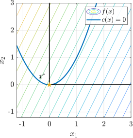
(a) The MPEC (16).

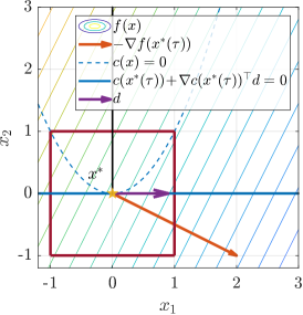
(b) LPEC (17) $\rho=1$.

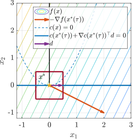
(c) LPEC (17) with $\rho=0.5$.

Figure 1: Illustration of Example 3.1. If a constraint qualification does not hold, the LPEC cannot verify B-stationary.

Example 3.1

Consider the following MPEC:

$$\underset{x\in{\mathbb{R}}^{2}}{\mathrm{min}}\;\quad -2x_{1}+x_{2}$$

s.t. $$x_{2}-x_{1}^{2}\geq 0$$

$$0\leq x_{1}\perp x_{2}\geq 0$$

The point $x^{*}=(0,0)$ is the global optimum of this problem and thus B-stationary. It can be seen that the tangent cone of this problem is ${\mathcal{T}}_{\Omega}(x^{*})=\{d\in{\mathbb{R}}^{2}\mid d_{1}=0,d_{2}\geq 0\}$. The corresponding LPEC reads as:

$$\underset{d\in{\mathbb{R}}^{2}}{\mathrm{min}}\;\quad -2d_{1}+d_{2}$$ (17a)

s.t. $$d_{2}\geq 0$$ (17b)

$$0\leq d_{1}\perp d_{2}\geq 0$$ (17c)

$$\|d\|_{\infty}\leq\rho.$$ (17d)

Clearly, ${\mathcal{T}}_{\Omega}(x^{*})\subset\mathcal{F}_{\Omega}(x^{*})$, which means that the MPEC-Abadie CQ does not hold at $x^{*}$. The only solution of (17) is $d=(\rho,0)$. Therefore, this LPEC cannot verify B-stationarity for any $\rho>0$. Fig. 1 illustrates the feasible sets of the MPEC and the LPEC for different $\rho$.

Next, we directly compare the two LPEC formulations and highlight some of their strengths and weaknesses in two examples.

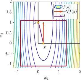
(a) $\rho=1.1$.

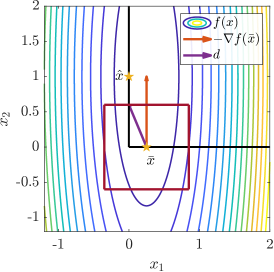
(b) $\rho=0.6$.

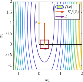
(c) $\rho=0.2$.

Figure 2: Illustration of the MPEC  (18). The yellow stars denote the two stationary points. The figure illustrates the LPEC’s (13) trust region, objective gradient, and optimal solution $d$ for different values of $\rho$.

Example 3.2 (Verifying B-stationarity)

Consider the following MPEC:

$$\min_{x\in{\mathbb{R}}^{2}}\ (ax_{1}-1)^{2}+(x_{2}-1)^{2}\quad\textnormal{s.t.}\quad 0\leq x_{1}\perp x_{2}\geq 0,$$ (18)

with $a>0$. This problem has two B-stationary points $\bar{x}=(\frac{1}{a},0)$ and $\hat{x}=(0,1)$, with $f(\bar{x})=f(\hat{x})=1$. We want to verify the B-stationarity of $\bar{x}$ with an LPEC solver that returns a globally optimal solution (which we often do in practice, cf. Section 3.2.2). Figure 2 illustrates this situation. For $\rho>\frac{1}{a}$, the solution of the full LPEC (13) will select the other branch, with the feasible set $x_{1}=0,x_{2}\geq 0$. However, the local optimum of this BNLP has the same objective value as the initial BNLP and the step will be rejected and the trust region radius reduced. The steps will be rejected until $\rho<\frac{1}{a}$, which for $a\ll 1$ may require many steps. On the other hand, the reduced LPEC (12) is just an LP and the B-stationary point is verified after the first LP is solved. For $\rho<\frac{1}{a}$, the full and reduced LPEC have the same feasible set, cf. Lemma 3.1.

A straightforward way to identify a B-stationary point in the example above is to exploit the fact that if a local optimizer of a BNLP $x^{*}$ has an empty biactive set ${\mathcal{I}}_{00}(x^{*})=\emptyset$, then this point is B-stationary. However, in practice, on a finite precision machine, the active sets must be determined with some threshold, e.g.,

$${\mathcal{I}}_{0+}^{\epsilon}(x)=\{i\mid x_{1,i}\leq\epsilon,x_{2,i}>\epsilon\},$$ (19a)

$${\mathcal{I}}_{+0}^{\epsilon}(x)=\{i\mid x_{1,i}>\epsilon,x_{2,i}\leq\epsilon\},$$ (19b)

$${\mathcal{I}}_{00}^{\epsilon}(x)=\{i\mid x_{1,i}\leq\epsilon,x_{2,i}\leq\epsilon\}.$$ (19c)

If in (18), one has $\epsilon>\frac{1}{a}$, a wrong conclusion about stationarity will be made, whereas the full LPEC does not need active set identification and always correctly identifies the B-stationary point.

In the next example, we show one more advantage and disadvantage of the full over the reduced LPEC.

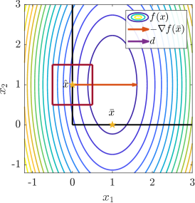
(a) $\rho=0.6$.

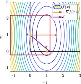
(b) $\rho=1.2$.

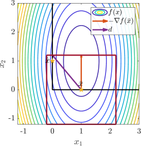
(c) $\rho=1.2$.

Figure 3: Illustration of the MPEC  (20). The yellow stars denote the two stationary points. The figure illustrates the LPEC’s (13) trust region, objective gradient, and optimal solution $d$ for different values of $\rho$ at different stationary points.

Example 3.3 (Finding a better objective value)

Consider the following MPEC:

$$\min_{x\in{\mathbb{R}}^{2}}\ 4(x_{1}-1)^{2}+(x_{2}-1)^{2}\quad\textnormal{s.t.}\quad 0\leq x_{1}\perp x_{2}\geq 0,$$ (20)

This problem has two B-stationary points $\bar{x}=(1,0)$ and $\hat{x}=(0,1)$ with the respective objective values $f(\bar{x})=1$ and $f(\hat{x})=4$. In Fig. 3a, if $\rho$ is sufficiently small or the reduced LPEC is used, the point $\hat{x}$ with $f(\hat{x})=4$ is verified as B-stationary point. On the other hand, with a larger trust region radius, as depicted in Fig. 3b, the globally optimal solution of the full LPEC identifies a BNLP with a lower objective value $f(\bar{x})=1$. Conversely, if we start at $\bar{x}$, the full LPEC can identify a BNLP with a larger objective, as depicted in Fig. 3c. However, this step will be rejected, and the trust region radius reduced until $\bar{x}$ is verified as B-stationary.

We make several observations from this example. First, solving the full LPEC to global optimality can help to find an objective with a lower value. Of course, as illustrated in Fig. 3c, there is no guarantee that this will always be the case. Second, if the trust region is not small enough, there is no guarantee that the descent direction corresponding to the global optimum of the LPEC leads to a BNLP with a lower objective value. Third, observe that when starting from $\hat{x}$ and then solving the BNLP predicted by the full LPEC as in Fig. 3b, the point $\hat{x}$ is not a feasible initial guess for the new BNLP, which may lead to step rejection if an NLP solver is not able to solve the new BNLP.

Next, we give sufficient conditions under which an ${\mathrm{LPEC}}(x^{k},\rho)$ predicts a BNLP for which $x^{k}$ is always a feasible point.

Lemma 3.2

Let $x^{k}\in\Omega$ be a feasible point of the MPEC (1) and suppose that the MPEC-Abadi CQ holds at this point. Let $d$ be any feasible point of the $\mathrm{LPEC}(x^{k},\rho)$ in (13) for $\rho\in(0,\bar{\rho})$, where $\bar{\rho}$ is defined in (14). Then $x^{k}$ is feasible in $\mathrm{BNLP}({\mathcal{I}}_{1}(x^{k}+d),{\mathcal{I}}_{2}(x^{k}+d))$.

Proof. It follows from Lemma 3.1 that for $\rho\in(0,\bar{\rho})$ both the full and reduced LPEC have the same feasible set. The relation (10) is also true for the respective tangent cones of the MPEC and auxiliary NLPs. Moreover, due to the MPEC-Abadi CQ, the relation (10) also holds for the MPEC-linearized feasible cones, i.e., the feasible set of the ${\mathrm{LPEC}}(x^{k},\rho)$. Thus, the proof follows directly from (10). ∎

Note that, since only feasible points $d$ are needed in Lemma 3.2, the assertion is true if we replace the cost gradient $\nabla f(x^{k})$ in $\mathrm{LPEC}(x^{k},\rho)$ with any vector $a\in{\mathbb{R}}^{n}$. Lemma 3.2 will be of great importance in the convergence analysis of MPECopt done in Section 4.

In summary, the full LPEC is easy to formulate at both feasible and infeasible points. The reduced LPEC is more suitable for feasible points and may be easier to solve. The full LPEC can find a better local optimizer at the cost of starting the next BNLP from an infeasible point. For a sufficiently small trust region radius, the feasible sets of the two LPECs coincide. Moreover, any feasible point of a reduced LPEC leads to an active set guess that corresponds to a feasible BNLP. In conclusion, in a practical implementation, one should use the full LPEC with a reasonably small trust region radius.

3.2.2 On solving LPECs

The practical success of the proposed method depends on the efficient solution of LPECs. There exists several tailored LPEC methods Fang2010 ; Hu2012 ; JaraMoroni2020 ; JaraMoroni2018 , but their implementations are not readily available. Since LPECs are a special case of MPECs, they can also be solved with any of the regularization and penalty-based methods mentioned in Section 2.2. However, it may be non-trivial to deal with cases where these methods converge to spurious solutions and fail to verify B-stationarity.

A practical and straightforward approach to solving LPECs (13) is to reformulate them as an equivalent mixed-integer linear program (MILP), which can be expressed as follows Hu2012 :

$$\underset{{d\in{\mathbb{R}}^{n},\ y\in\{0,1\}^{m}}}{\mathrm{min}}\;\quad \nabla f(x^{k})^{\top}d$$ (21a)

s.t. $$c(x^{k})+\nabla c(x^{k})^{\top}d\geq 0,$$ (21b)

$$0\leq x_{1,i}\!+\!d_{1,i}\!\leq\!yM, \forall i\in\{1,\ldots,m\},$$ (21c)

$$0\leq x_{2,i}\!+\!d_{2,i}\!\leq\!(e-y)M, \forall i\in\{1,\ldots,m\},$$ (21d)

$$\|d\|_{\infty}\leq\rho,$$ (21e)

where $e$ is a vector of ones with appropriate dimensions, and $M$ is a sufficiently large positive constant. The constraints (21c) and (21d) correspond to the big-M reformulation of the complementarity constraints in (13c). The binary variables $y\in\{0,1\}^{m}$ effectively select one of the branches of the L-shaped set introduced by the complementarity constraints.

The MILP (21) can be solved with state-of-the-art commercial and open-source solvers such as Gurobi Gurobi or HiGHS Huangfu2018 . In general, due to the exponential complexity of MILPs, this can be computationally expensive. Moreover, big-M formulations can be inefficient as they can lead to rather loose relaxations Hu2008 . In the special case of (21), we argue that the MILP can usually be solved very efficiently in practice for several reasons.

Observe that the constraint (21e) makes the feasible set of the MILP compact. Moreover, for feasible points $x^{k}$, the trust region radius $\rho$ can be arbitrarily small, leading to tight relaxations of the MILP. For small $\rho$, the trust region constraint (21e) always dominates the bounds on $d$ implied by the big-M constraints (21c) and (21d). Therefore, a large $M$ does not lead to loose relaxations of the MILP. Thus, $M$ only needs to be large enough to ensure the feasibility of  (21c)-(21d) and that is not tighter than (21e). One choice is $M=\max((x_{1}^{k},x_{2}^{k}))+\rho$. Furthermore, given a feasible complementarity pair, e.g. from the previous BNLP or LPEC solution, we can construct a feasible binary vector $y$, leading to a good upper bound.

All this together typically leads to faster solution times in practice. As it will be shown in Section 5, the cumulative time spent solving MILPs (21) is only a small fraction of the overall solution time. Moreover, it will also be seen that the MILP formulations for LPECs lead to much smaller computation times than the corresponding regularization-based methods.

We mention also the special but not so uncommon case when a point $x^{*}\in\Omega$ is an S-stationary point. In this case, the MILP is especially easy to solve, because the solution of the relaxed MILP – which is an LP obtained by setting $y\in[0,1]^{m}$ instead of $y\in\{0,1\}^{m}$ – already solves the MILP. This means that the verification of a B-stationary point in this case reduces to a single LP solve. The next lemma formalizes this assertion.

Lemma 3.3

Let $x^{*}\in\Omega$ be a S-stationary point of the MPEC (1). For a sufficiently small $\rho>0$, a global minimizer of the relaxed MILP (21) is $d=0$, and $y\in[0,1]^{m}$ such that (21c) and (21d) hold. Moreover, any $y\in\{0,1\}^{m}$ that satisfies (21c) and (21d) and $d=0$ are a global minimizer of the MILP (21).

Proof. It follows from Theorem 2.1 that if $x^{*}\in\Omega$ is S-stationary, it is also B-stationary, hence $d=0$ is a local minimizer of the ${\mathrm{LPEC}}(x^{*},\rho)$ in (13). For a sufficiently small $\rho>0$, $d=0$ is also a global minimizer of ${\mathrm{LPEC}}(x^{*},\rho)$. Now, since $x^{*}$ is S-stationary, it is also a stationary point of the so-called relaxed NLP, which is obtained by replacing (9e) in the TNLP by $x_{1,i},x_{2,i}\geq 0,i\in{\mathcal{I}}_{00}(x^{*})$ Scheel2000 . This also means that the LP obtained by linearizing all functions of the relaxed NLP has $d=0$ as its global minimizer. Adding a trust region constraint with $\rho>0$ on the step $d$ does not change the solution of this LP, which reads as:

$$\underset{{d\in{\mathbb{R}}^{n}}}{\mathrm{min}}\;\quad \nabla f(x^{k})^{\top}d$$ (22a)

s.t. $$c(x^{k})+\nabla c(x^{k})^{\top}d\geq 0,$$ (22b)

$$x_{1,i}+d_{1,i}=0,\ x_{2,i}+d_{2,i}\geq 0,\; \forall i\in\mathcal{I}_{0+}(x^{*}),$$ (22c)

$$x_{1,i}+d_{1,i}\geq 0,\ x_{2,i}+d_{2,i}=0,\; \forall i\in\mathcal{I}_{+0}(x^{*}),$$ (22d)

$$x_{1,i}+d_{1,i}\geq 0,\ x_{2,i}+d_{2,i}\geq 0,\; \forall i\in\mathcal{I}_{00}(x^{*}),$$ (22e)

$$\|d\|_{\infty}\leq\rho$$ (22f)

Now by applying similar reasoning as in the proof of Lemma 3.1, it can be seen that by relaxing $y\in\{0,1\}^{m}$ to $y\in[0,1]^{m}$ in  (21), and for a sufficiently small $\rho>0$, the feasible sets of relaxed MILP  (21) and the LP (22) coincide for all $d\in{\mathbb{R}}^{n}$ components. Since $y$ does not enter the objective, $d=0$ is also a minimizer of the relaxed MILP. Finally, since the ${\mathrm{LPEC}}(x^{*},\rho)$ in (13) has only one global minimum, we conclude that $d=0$ and any $y$ that satisfies (21c) and (21d) are a global minimizer of the equivalent MILP (21). A vector $y\in\{0,1\}^{m}$ is trivially obtained from the evaluation of (21c) and (21d) with $d=0$ and $x^{*}$. ∎

Once the MILP (21) is solved, if $d\neq 0$ we need to identify the active sets ${\mathcal{I}}_{1}(x^{k}+d)$ and ${\mathcal{I}}_{2}(x^{k}+d)$, which requires some partition of ${\mathcal{I}}_{00}(x^{k}+d)$. There is some ambiguity here, and in our implementation, we use the MILP solution and define

$${\mathcal{I}}_{1}(x^{k}+d)=\{i\mid y_{i}=0\},\ {\mathcal{I}}_{2}(x^{k}+d)=\{i\mid y_{i}=1\}.$$

We highlight that MILP solvers usually solve (21) to global optimality. For the presented method, however, it is sufficient that the LPEC solver either verifies $d=0$ as a local optimizer or finds a descent direction $d$ that predicts an active set and a corresponding BNLP with a lower objective value.

In practice, the global solution may be on an edge of the feasible set, where it is possible to have $\nabla f(x^{k})^{\top}d=0$ with $d\neq 0$, cf. Fig 3a for an example. In such cases, we consistently select $d=0$.

Remark 3.1 (On Algorithm 1 and mixed-integer algorithms)

Many mixed-integer nonlinear programming (MINLP) methods Belotti2013 , solve a sequence of NLPs and MILPs, just like Algorithm 1. Therefore, we highlight their major conceptual differences. Using the big-M reformulation, any MPEC (1) can be reformulated into a MINLP. Most MINLP methods converge to the global optimum when the relaxed integer problem is a convex problem, Algorithm 1 does not. This can be seen in the MPEC example in (20). It can be verified that the equivalent MINLP, obtained via the big-M reformulation, after relaxing the binary variable from $y\in\{0,1\}^{m}$ to $y\in[0,1]^{m}$ results in a convex quadratic program. We have seen in Example 3.3, that the Algorithm 1 does not always converge to the global optimum of the MPEC, but only to a B-stationary point. In summary, Algorithm 1 is not a MINLP algorithm, and the MILP solvers are just a tool to solve LPECs.

3.3 Phase I: Finding a feasible branch NLP

In this section, we introduce two algorithms to find an initial consistent BNLP and its corresponding solution $x^{0}$, or to certify (local) infeasibility of (1) if this is impossible. The first algorithm solves a relaxed NLP, and the second explicitly minimizes the constraint violation subject to the complementarity constraint (1c).

3.3.1 Regularization-based approach

Even though regularization-based methods may not always find B-stationary points, they can be efficient in finding (almost) feasible points. In this section, we present a Phase I method that combines solving LPECs with regularization-based methods described in Section 2.2. In our exposition, we focus on Scholtes’ global relaxation method, cf. Section 2.2. We compute $x^{*}(\tau)$, a stationarity point of Reg($\tau$), which is not necessarily feasible for the MPEC (1). Next, an LPEC is constructed at $x^{*}(\tau)$ (for some $\tau>0$), and the solution of the LPEC is then used to find an active set corresponding to a feasible BNLP. Such an approach is motivated by Lemma 3.2, and the following straightforward fact.

Lemma 3.4

Consider the MPEC (1). Let $c$ be an affine function, $x\in{\mathbb{R}}^{n}$, and $a\in{\mathbb{R}}^{n}$ any nonzero vector. Then, for a sufficiently large $\rho$ and for any local minimizer $d$ of the LPEC:

$$\underset{d\in{\mathbb{R}}^{n}}{\mathrm{min}}\;\quad a^{\top}d$$ (23a)

s.t. $$c(x)+\nabla c(x)^{\top}d\geq 0,$$ (23b)

$$0\leq x_{1,i}+d_{1,i}\perp x_{2,i}+d_{2,i}\geq 0, \forall i\in\{1,\ldots,m\},$$ (23c)

$$\|d\|_{\infty}\leq\rho,$$ (23d)

it follows, that $x+d\in\Omega$. Additionally, if this LPEC is infeasible for all sufficiently large $\rho>0$, then the MPEC (1) is also infeasible.

This lemma trivially follows from the fact that for $x\in\Omega$ the LPEC and the MPEC have the same feasible set, hence an LPEC with any objective can identify a feasible BNLP. The trust-region radius $\rho>0$ has just to be large enough such that the complementarity constraints can be satisfied. In our implementation, for the objective, we take $a=\nabla f(x)$ (i.e., (23) reduces to (13)), but other choices such as minimizing the distance to the feasible set are also possible.

Now, if the function $c$ is nonlinear, and we have an almost feasible point $x$, we expect that the LPEC (23) can identify a feasible BNLP. We prove below in Theorem 4.1 that this is indeed the case.

On the other hand, certifying that a general nonconvex optimization problem is infeasible is difficult. Therefore, most NLP methods detect so-called local infeasibility, which is defined as follows. If the globalization strategy of an NLP method cannot make sufficient progress toward finding a feasible point, then an auxiliary NLP – which usually minimizes the constraint violation – is solved Fletcher2002 ; Waechter2006 . If a local minimizer (or stationary point) of this auxiliary NLP is not a feasible point of the original NLP, then the original problem is declared to be locally infeasible.

We highlight a fact about infeasibility detection with the regularization-based approach.

Lemma 3.5

Regard the MPEC (1) and the corresponding $\mathrm{Reg}(\tau)$ in  Reg($\tau$) for some $\tau>0$. If $\mathrm{Reg}(\tau)$ is locally infeasible then the same holds for the MPEC (1).

Proof. This follows from the fact that the feasible set of $\mathrm{Reg}(\tau)$ is a superset of $\Omega$. ∎

On the other hand, if Reg($\tau$) is feasible for all $\tau$, then also the MPEC (1) is feasible as well. In a practical implementation, we compute a finite sequence of $x^{*}(\tau^{k})$ for $k=0,\ldots,N^{\tau}$, and solve the $\mathrm{LPEC}(x^{*}(\tau^{k}),\rho)$. We expect that if $\tau^{k}$ is sufficiently small, then the feasible set of $\mathrm{LPEC}(x^{*}(\tau^{k}),\rho)$ is locally a good approximation of the original feasible set. It is not known a priori how small $\tau^{k}$ and how large $\rho$ must be for a feasible BNLP to be identified. The following example illustrates how an LPEC can fail to identify a feasible BNLP if $\tau$ is not sufficiently small.

Example 3.4

Consider the following MPEC:

$$\underset{x\in{\mathbb{R}}^{2}}{\mathrm{min}}\;\quad -2x_{1}+x_{2}$$

s.t. $$-x_{1}-(x_{2}-a)^{2}+1\geq 0$$

$$0\leq x_{1}\perp x_{2}\geq 0$$

with $a>1$. In the example, we set $a=1.1$. If $\tau$ is not small enough, then the LPEC (13) has feasible branches, which are infeasible for the original MPEC. Fig. 4 illustrates two sample solutions for $\mathrm{Reg}(\tau)$ and the corresponding $\mathrm{LPEC}(x^{*}(\tau),\rho)$. In this example, the smaller the parameter $a$ is the smaller $\tau$ must become.

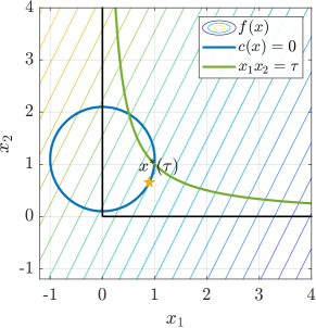
(a) $\tau=1$.

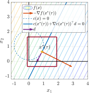
(b) $\tau=1$.

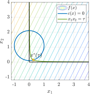
(c) $\tau=0.04$.

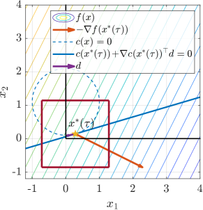
(d) $\tau=0.04$.

Figure 4: Illustrating of Example 3.4, where the LPEC (13) can correctly and wrongly identify a feasible BNLP depending on the linearization point $x^{*}(\tau)$.

Algorithm 2 Regularization-based Phase I of MPECopt

1:Input: $x^{0}$, $\rho_{I}>0$, $\kappa\in(0,1)$, $\tau^{0}>0$, $N^{\tau}>1$ $k=0,\ldots,N^{\tau}$

2:Solve $\mathrm{Reg}(\tau^{k})$ for $x^{*}(\tau^{k})$ $\mathrm{Reg}(\tau^{k})$ locally infeasible

3:break $\triangleright$ MPEC locally infeasible $x^{*}(\tau^{k})\in\Omega$

4:break; return $x^{0}=x^{*}(\tau^{k})$ $\triangleright$ $\mathrm{Reg}(\tau^{k})$ solution feasible for MPEC $h_{\perp}(x(\tau^{k}))<\rho_{I}$

5:Solve $\mathrm{LPEC}(x^{*}(\tau^{k}),\rho_{I})$ for $d^{k}$ $d^{k}$ exists

6:Solve $\mathrm{BNLP}({\mathcal{I}}_{1}(x^{*}(\tau^{k})+d^{k}),{\mathcal{I}}_{2}(x^{*}(\tau^{k})+d^{k}))$ for $x^{0}$. Solution exists

7:break, return $x^{0}$ $\triangleright$ feasible point found

8:$\tau=\kappa\tau$. $\triangleright$ no feasible LPEC/BNLP found, reduce homotopy parameter

A regularization-based Phase I is summarized in Algorithm 2. In a practical implementation, a point is declared feasible if the constraint residual is below a certain tolerance. Formally, we require $h(x)\leq\texttt{tol}_{h}$, where $h(x)$ is the total infeasibility defined as:

$$h(x)=\|(h_{c}(x),h_{\perp}(x))\|_{\infty},\ h_{c}(x)=\|c^{-}(x)\|_{\infty},\ h_{\perp}(x)=\max(|\min(x_{1},x_{2})|),$$

with $c^{-}(x)=\min(0,c(x))$.

In our implementation, we take a finite number $N^{\tau}$ of homotopy steps. If the number of steps is large enough, Algorithm 2 eventually finds a feasible point or certifies local infeasibility. If $\mathrm{Reg}(\tau^{k})$ is infeasible, or its solution is already feasible for the MPEC, the algorithm terminates. Otherwise, the solution $x^{*}(\tau^{k})$ is used to construct ${\mathrm{LPEC}}(x^{*}(\tau^{k}),\rho_{I})$. The trust region radius $\rho_{I}$ must be sufficiently large to ensure that this LPEC is feasible. Note that a solution of $\mathrm{Reg}(\tau^{k})$ already satisfies the general inequality constraints, i.e., $c(x^{*}(\tau^{k}))\geq 0$. Therefore, we focus on values that make the complementarity constraint in the LPEC feasible. In our implementation, we use a fixed trust region radius with $\rho_{I}>0$. The smallest value of $\rho_{I}$ needed to make the LPEC feasible is $\rho_{I}>h_{\perp}(x^{*}(\tau^{k}))$, and we attempt to solve the LPEC only if this inequality is satisfied. If the LPEC is infeasible, the homotopy parameter is reduced, to obtain a better linearization point $x^{*}(\tau^{k})$. If a solution to the LPEC is found, Algorithm 2 attempts to solve the corresponding BNLP. If this is successful, a feasible point is found, otherwise, the homotopy parameter is reduced to obtain a better linearization point $x^{*}(\tau^{k+1})$. We prove in Theorem 4.1 that if $x^{*}(\tau^{k})$ is sufficiency close to a feasible point $x\in\Omega$, then the $\mathrm{BNLP}({\mathcal{I}}_{1}(x^{*}(\tau^{k})+d^{k}),{\mathcal{I}}_{2}(x^{*}(\tau^{k})+d^{k}))$ is a feasible BNLP, where $d^{k}$ is a feasible point of $\mathrm{LPEC}(x^{*}(\tau^{k}),\rho^{I})$ . In our implementation, every $\mathrm{Reg}(\tau^{k})$, for $k>0$ is initialized with the solution of $\mathrm{Reg}(\tau^{k-1})$, and $\mathrm{BNLP}({\mathcal{I}}_{1}(x^{*}(\tau^{k})+d),{\mathcal{I}}_{2}(x^{*}(\tau^{k})+d))$ is initialized with $x^{*}(\tau^{k})$. The constants in our implementation are $\kappa=0.1$, $\tau^{0}=1$, $N^{\tau}=12$, ${\rho}^{I}=10^{-1}$, and $\texttt{tol}_{h}=10^{-10}$.

Solving the LPECs in Algorithm 2 can be computationally expensive. Thus, we may look for other strategies for guessing the active sets ${\mathcal{I}}_{0+}^{0}$, ${\mathcal{I}}_{0+}^{0}$, and ${\mathcal{I}}_{00}^{0}$ corresponding to a feasible point $x^{0}$ which is close to $x^{*}(\tau^{k})$. Some of such strategies are studied in Lin2006 . They all resemble the active set guessing in (19), but where $\epsilon$ is replaced by some function of $x$ and $\tau$. These strategies can be effective if the set ${\mathcal{I}}_{00}^{0}$ is an empty set. Otherwise, strong assumptions are needed for a correct active set identification if ${\mathcal{I}}_{00}\neq\emptyset$. Unfortunately, slightly over or underestimating ${\mathcal{I}}_{00}^{0}$ can quickly lead to an infeasible BNLP. For example, taking ${\mathcal{I}}_{00}=\{1\}$ in Example 3.4, and doing a wrong partition leads to an infeasible BNLP.

For the sake of comparison, we implement a simple LPEC-free strategy, which replaces lines 4-5 in Algorithm 2 with the following active set identification strategy. We use  (19) and set $\epsilon=\tau$. The biactive set is split into ${\mathcal{D}}_{1}(x(\tau))=\{i\in{\mathcal{I}}_{00}^{\tau}\mid x^{*}_{1,i}(\tau)<x^{*}_{2,i}(\tau)\}$ and ${\mathcal{D}}_{2}(x(\tau))=\{i\in{\mathcal{I}}_{00}^{\tau}\mid x^{*}_{1,i}(\tau)\geq x^{*}_{2,i}(\tau)\}$, which finally results in the following partition for the BNLP:

$${\mathcal{I}}_{1}=\{i\mid x^{*}_{1,i}(\tau)<x^{*}_{2,i}(\tau)\},\quad{\mathcal{I}}_{2}=\{i\mid x^{*}_{1,i}(\tau)\geq x^{*}_{2,i}(\tau)\}.$$ (24)

Note that in the overall algorithm, LPECs are still needed in Phase II.

3.3.2 Feasibility-based approach

A common approach for finding a feasible point in many optimization algorithms is to solve an auxiliary problem that minimizes the total infeasibility Fletcher2002 ; Waechter2006 .

We propose to solve the following feasibility problem:

$$\underset{x\in{\mathbb{R}}^{n}}{\mathrm{min}}\;\quad \|c^{-}(x)\|$$ (25a)

s.t. $$0\leq x_{1}\perp x_{2}\geq 0,$$ (25b)

where $c^{-}(x)=\min(0,c(x))$ is the component-wise infeasibility of the inequality constraints. A crucial property of this MPEC is that it is always feasible, and we can directly apply Phase II of MPECopt to it. However, its objective is nondifferentiable. We discuss several special cases (in which we specify the norm in (25)), where this problem can be made smooth and solved efficiently in practice.

First, we can replace the objective of  (25) with $\|c^{-}(x)\|_{2}^{2}$, which is now once continuously differentiable. This allows us to apply a sequential LPEC method for MPECs with bound constraints Kirches2022 . Remarkably, the LPEC, in this case, has only bound and complementarity constraints, and it can be solved to global optimality with linear complexity (Kirches2022, , Proposition 2.4). However, the convergence rate of sequential LPEC methods is usually slow, and we may want to use Phase II of MPECopt directly. If there are only equality constraints but no inequality constraints in (1), then the squared two norm objective is twice continuously differentiable, and one can use Phase II of MPECopt combined with the fast explicit LPEC solver from (Kirches2022, , Proposition 2.4). In the presence of inequality constraints, one has to solve the usual LPEC as in Eq. (13).

Second, if we use the $\ell_{1}$-norm, a well-known smooth reformulation is:

$$\underset{x\in{\mathbb{R}}^{n},s\in{\mathbb{R}}^{n_{c}}}{\mathrm{min}}\;\quad \sum_{i=1}^{n_{c}}s_{i}$$ (26a)

s.t. $$c_{i}(x)\geq-s_{i}, \forall i\in\{1,\ldots,n_{c}\}$$ (26b)

$$0\leq x_{1}\perp x_{2}\geq 0,$$ (26c)

$$s\geq-s^{\mathrm{lb}}\,e,$$ (26d)

where $e\in{\mathbb{R}}^{n_{c}}$ is a vector of all ones and $s^{\mathrm{lb}}$ is a nonnegative constant set here to zero. The $\ell_{\infty}$ norm is obtained similarly if we use a scalar slack variable instead of $s\in{\mathbb{R}}^{n_{c}}$. If we wish to find a strictly feasible point for the general inequality constraints, we can set $s^{\mathrm{lb}}$ to some positive number, and terminate the algorithm as soon as all components of $s$ are below zero. Since the MPEC (26) is always feasible we treat it with Phase II of MPECopt, outlined in the next section. If Phase II terminates with a B-stationary point and some $s_{i}>0$, we conclude that the MPEC is locally infeasible. If one would solve the problem to global optimality, with some $s_{i}>0$ being the optimal solution, then the MPEC is infeasible.

A special case is if the functions $c$ are concave. Then every BNLP of (26) is a convex optimization problem. If every BNLP has a solution with at least one $s_{i}>0$, then the MPEC is globally infeasible. We mention one more special case, which is hard to verify in practice. If the linearization of $c$ at $x$ is an inner approximation of $c(x)\geq 0$. Then it is sufficient to solve a single LPEC to find a feasible point of the MPEC.

3.4 Phase II: Computing a B-stationary point

Most ingredients of Phase II are already listed in Algorithm 1. A version with more implementation details is given in Algorithm 3.

Algorithm 3 Phase II of MPECopt

1:Input: $x^{0}\in\Omega$, $\rho^{0}\in[\rho^{\mathrm{lb}},\rho^{\mathrm{ub}}]$, $\gamma^{\mathrm{L}}\in(0,1)$, $\gamma^{\mathrm{U}}>1$, $N^{\mathrm{out}}$, $N^{\mathrm{in}}$ $k=0,\ldots,N^{\mathrm{out}}$ $\triangleright$ major/outer iterations

2:Possibly reset trust region radius $\rho^{k,0}\in[\rho^{\mathrm{lb}},\rho^{\mathrm{ub}}]$; $l=0,\ldots$ $\triangleright$ minor/inner iterations

3:Solve $\mathrm{LPEC}(x^{k},\rho^{k,l})$ for $d^{k,l}$ $\|d_{\mathrm{L}}^{k,l}\|_{\infty}\leq\texttt{tol}_{\mathrm{B}}$

4:terminate $\triangleright$ B-stationary point found $l=0$ or ${\mathcal{I}}_{1}(x^{k}+d^{k,l})\neq{\mathcal{I}}_{1}(x^{k}+d^{k,l-1})$

5:Solve $\mathrm{BNLP}({\mathcal{I}}_{1}(x^{k}+d^{k+l},{\mathcal{I}}_{1}(x^{k}+d^{k+1})$ to obtain $x^{k,l}$ BNLP solver failed or $f(x^{k,l})\geq f(x^{k})$

6:${\rho}^{k,l+1}={\gamma^{\mathrm{L}}\rho^{k,l}}$; $\triangleright$ reduce TR radius

7:${\rho}^{k,l+1}={\gamma^{\mathrm{U}}\rho^{k,l}}$

8:$x^{k+1}=x^{k,l}$; break inner for-loop; $\triangleright$ step accepted

9:${\rho}^{k,l+1}={\gamma^{\mathrm{L}}\rho^{k,l}}$ $\triangleright$ reduce TR radius

In the next section, we prove that this algorithm terminates after a finite number of iterations. In a practical implementation, we allow a predetermined maximum number of inner and outer iterations, and if this number is not large enough to find a B-stationary point, then the solver returns an according message. A point is declared to be B-stationary if $\|d^{k,l}\|_{\infty}\leq\texttt{tol}_{\mathrm{B}}$, where $\texttt{tol}_{\mathrm{B}}=10^{-8}$. The number of inner iterations $N^{\mathrm{in}}$ must be such that $\rho^{k,l}$ cannot be less than $\texttt{tol}_{\mathrm{B}}$. In the inner iterations, the BNLP is solved again only if the active set LPEC solution predicts new active sets ${\mathcal{I}}_{1}(x^{k}+d^{k,l})$ and ${\mathcal{I}}_{2}(x^{k}+d^{k,l})$, compared to the previous LPEC solution $x^{k}+d^{k,l-1}$. A new iterate is accepted only if it strictly reduces the objective of the MPEC (1). To reduce conservatism, the radius of the trust region can be rested or increased after each successful major iteration but this is not necessary for convergence.

Recall that a B-stationary point of an MPEC is also a stationary point of all corresponding BNLPs and the TNLP, cf. Eq. (10). Therefore, instead of solving the $\mathrm{BNLP}({\mathcal{I}}_{1}(x^{k}+d^{k+l},{\mathcal{I}}_{1}(x^{k}+d^{k+1})$, MPECopt would also converge if one solves a sequence of TNLPs based on the estimate ${\mathcal{I}}_{0+}(x^{k}+d^{k+l})$, ${\mathcal{I}}_{+0}(x^{k}+d^{k+l})$ and ${\mathcal{I}}_{00}(x^{k}+d^{k+l})$. In a practical implementation, we prefer to solve a sequence of BNLPs over TNLPs because of the following two reasons. First, if due to rounding errors the set ${\mathcal{I}}_{00}(x^{k}+d^{k+l})$ is computed wrongly, one can obtain infeasible subproblems. This can be avoided by estimating the BNLP index sets directly from the MILP solution, as discussed in Section 3.2.2. Second, the feasible set of all BNLPs is a superset of the TNLP, which may allow us to find better descent directions from non-stationary points.

In our implementation of Algorithm 3, we reset the trust region after every successful inner iteration and use the following constants: $\rho^{0}=10^{-3}$, $\rho^{\mathrm{lb}}=10^{-7}$, $\rho^{\mathrm{ub}}=100$, $\gamma^{\mathrm{L}}=0.1$, $\gamma^{\mathrm{U}}=10$, $N^{\mathrm{out}}=25$, and $N^{\mathrm{in}}=4$.

4 MPECopt convergence proof

This section provides the convergence proof of the MPECopt method. Before stating the main result, we state the main assumption and some auxiliary results.

4.1 Assumptions

MPECopt can use any globalized NLP solvers that satisfy the following assumption.

Assumption 4.1 (NLP solver)

Consider a nonlinear program

$$\min_{x}f(x)\quad\textnormal{s.t.}\quad g(x)\geq 0,$$ (27)

where $f:{\mathbb{R}}^{n}\to{\mathbb{R}}$ and $g:{\mathbb{R}}^{n}\to{\mathbb{R}}^{n_{g}}$ are twice continuously differentiable functions. Starting from an initial guess $x^{0}\in{\mathbb{R}}^{n}$, an NLP solver returns a stationary point $x^{*}$ or a certificate of local infeasibility. Moreover, if $x^{0}$ is a feasible but not stationary point of (27), then it returns a point $x^{*}$ such that $f(x^{*})<f(x^{0})$.

The NLP (27) is a generic problem that covers all NLPs solved in this paper, including (8), Reg($\tau$) and the BNLPs arising in Section 3.3.2. This assumption is met in practice by many globalized NLP solver implementations, e.g. IPOPT Waechter2006 , filterSQP Fletcher2002b , SNOPT Gill2005 and uno Vanaret2024 , to name a few. Methods that can be efficiently warm-started may profit from the fact that in Phase II all iterates are feasible.

The most restrictive requirement is that starting from a feasible point $x^{0}$, the NLP solver finds $x^{*}$ such that $f(x^{*})<f(x^{0})$. It may happen that even starting from a feasible point, the NLP solver cannot find a point acceptable to a globalization strategy, i.e., better objective and sufficiently feasible. In such cases, a feasibility restoration phase is usually triggered Waechter2006 , which may return a point with a higher objective. However, we never observed this event in any of our extensive numerical experiments, and thus we do not treat this outcome further. A possible remedy is to add the constraint $f(x)\leq f(x^{k})$ to the current BNLP.

We state our requirements on the LPEC solver.

Assumption 4.2 (LPEC solver)

Let $x^{k}\in{\mathbb{R}}^{n}$ and $\rho>0$. The LPEC solver applied to $\mathrm{LPEC}(x^{k},\rho)$ satisfies the following:

• If $x^{k}\notin\Omega$, then it certifies that the LPEC is locally infeasible or returns a local minimizer $d\in{\mathbb{R}}^{n}$.

• If $x^{k}\in\Omega$ and $d=0$ is a local minimizer then this is certified. Otherwise, a local optimizer $d\neq 0$ such that $\nabla f(x^{k})^{\top}d<0$ is returned.

This assumption is always satisfied by globally solving the MILP (21), but it is clear that global optimality is not necessary.

We do not treat unbounded problems, and require the following assumption, which is satisfied by adding lower and upper bounds to all variables $x\in{\mathbb{R}}^{n}$.

Assumption 4.3

There exists a compact set $X$ such that for the feasible set $\Omega$ of the MPEC (1) it holds that $\Omega\subset X$.

In the proof below we often use Eq. (10). This relation also holds for the respective tangent cones of the MPEC, TNLP and the BNLPs. If a constraint qualification holds, this is also true for the MPEC-linearized feasible cones, which are used to define the feasible set of the LPECs. Thus, to avoid the degenerate case of Example 3.1 we require a weak constraint qualification.

Assumption 4.4

Let $x\in\Omega$ be a feasible point of the MPEC (1). Then the MPEC-Abadie CQ holds at this point.

Note that practical NLP solvers from Assumption 4.1 may need stronger CQs, e.g. the MFCQ for each BNLP, resulting in MPEC-MFCQ. However, as long as a solver can satisfy Assumption 4.1, we do not need to specify stronger assumptions for MPECopt.

4.2 Main convergence results

We start with a useful proposition. A similar result is available in Kirches2022 ; Leyffer2007 .

Proposition 4.1

Let $x\in\Omega$ be a feasible point for the MPEC (1), which is not B-stationary in the sense of Definition 2.1. Then there exists an $\epsilon>0$, a step $s\in{\mathbb{R}}^{n}$ with $\|s\|_{\infty}=1$ and a partition $({\mathcal{D}}_{1}(x),{\mathcal{D}}_{2}(x))$ of ${\mathcal{I}}_{00}(x)$ such that:

$$\nabla f(x)^{\top}s<-\epsilon,$$ (28a)

$$\nabla c_{i}(x)^{\top}s\geq\epsilon i\in{\mathcal{A}}(x),$$ (28b)

$$s_{1,i}=0, i\in{\mathcal{I}}_{0+}(x),$$ (28c)

$$s_{2,i}=0, i\in{\mathcal{I}}_{+0}(x),$$ (28d)

$$s_{1,i}=0,\ s_{2,i}\geq 0, i\in{\mathcal{D}}_{1}(x),$$ (28e)

$$s_{1,i}\geq 0,\ s_{2,i}=0, i\in{\mathcal{D}}_{2}(x).$$ (28f)

Proof. If $x$ is not a B-stationary point then it follows from (10) that it is not stationary for at least one BNLP. The assertion follows by regarding every corresponding LP piece. Since $d=0$ is not a solution for these LPs, then there exists a descent direction $s$ on at least one BNLP. ∎

Next, we show that an LPEC constructed at an almost feasible point can predict a feasible BNLP. In our implementation, such a point, and the corresponding LPEC are found via Algorithm 2.

Theorem 4.1

Let Assumptions 4.1-4.4 hold. Consider $x^{*}\in\Omega$ a feasible point of the MPEC (1), and $\tilde{x}\in X$ (not necessarily an element of $\Omega$) such that $\|\tilde{x}-x^{*}\|\leq\delta$. Then, there exist positive constants $\kappa$, $\epsilon$ such that for a sufficiently small $\delta$ the following interval is nonempty

$$\max\Big{\{}\frac{h_{c}(\tilde{x})}{\epsilon},h_{\perp}(\tilde{x})\Big{\}}\leq\rho\leq\kappa,$$ (29)

and for any $\rho$ from this interval the $\mathrm{LPEC}(\tilde{x},\rho)$ in (13) is feasible. Moreover, for any feasible point $d$ of this LPEC, it follows that $\mathrm{BNLP}({\mathcal{I}}_{1}(\tilde{x}+d),{\mathcal{I}}_{2}(\tilde{x}+d))$ is feasible as well.

Proof. Consider the case when $\tilde{x}\in\Omega$, i.e., $\delta=0$. The $\mathrm{LPEC}(\tilde{x},\rho)$ is always feasible for this point and let $d$ be an element of its feasible set. Now set $\kappa=\bar{\rho}$, where $\bar{\rho}$ is defined in (14). Then according to Lemma 3.2, for all $\rho\in(0,\kappa)$, every ${\mathrm{BNLP}}({\mathcal{I}}_{1}(\tilde{x}+d),{\mathcal{I}}_{2}(\tilde{x}+d))$ is feasible.

Next, we prove the assertion for $\tilde{x}\notin\Omega$. The main idea of the proof is to consider a feasible $x^{*}\in\Omega$, and to show that Lemma 3.2 is also true for points $\tilde{x}$ close enough to $x^{*}$. Denote by $\mathcal{B}(x,\rho)=\{d\in{\mathbb{R}}^{n}\mid\|d-x\|_{\infty}\leq\rho\}$ the $\ell_{\infty}$-ball centered at $x\in{\mathbb{R}}^{n}$ with the radius $\rho>0$.

First, we show that LPECs defined at points close to $x^{*}$ are also feasible under suitable conditions. Let $x^{*}\in\Omega$ be feasible but not B-stationary. It follows form Proposition 4.1 and the continuity of the functions $f$, and $c$, that there exists a neighborhood $\mathcal{N}^{*}=\mathcal{B}(x^{*},\kappa_{1})\cap X$, such that for all $\tilde{x}\in\mathcal{N}^{*}$ it holds that:

$$\nabla f(\tilde{x})^{\top}d<-\epsilon,\nabla c_{i}(\tilde{x})^{\top}s\geq 0,\ i\in{\mathcal{A}}(x^{*}).$$ (30)

Next, we prove that every ${\mathrm{LPEC}}(\tilde{x},\rho)$ for all $\tilde{x}\in\mathcal{N}^{*}$ and a suitable $\rho$ is feasible. We start first with the general inequality constraints and use an argument similar to (Chin2003, , Lemma 4). Take the step $d=\rho s$, which satisfies $\|d\|\leq\rho$, and consider the lineraization of the inequality constraints active at $x^{*}$:

$$c(\tilde{x})+\rho\nabla c_{i}(\tilde{x})^{\top}s\geq-h_{c}(\tilde{x})+\rho\epsilon, i\in{\mathcal{A}}(x^{*}).$$ (31)

The first term is lower bounded by the infeasibility of the inequality constraints, the second uses the fact that $\|s\|_{\infty}=1$ and (30). For the inequality constraints inactive at $x^{*}$, it follow from the continuity of $c$ that there exists positive constants $\gamma_{1}$ and $\gamma_{2}$ independent of $\tilde{x}$ such that $c(\tilde{x})\geq\gamma_{1}$ and $\nabla c_{i}(\tilde{x})^{\top}s\geq-\gamma_{2}$. Thus for the inactive constraints, we have

$$c(\tilde{x})+\rho\nabla c_{i}(\tilde{x})^{\top}s\geq\gamma_{1}-\rho\gamma_{2}, i\notin{\mathcal{A}}(x^{*}).$$ (32)

By requiring that the right-hand-side of  (31) and (32) are non-negative, we find that the linearized inequality constraints are feasible if $\rho$ satisfies:

$$\frac{h_{c}(\tilde{x})}{\epsilon}\leq\rho\leq\frac{\gamma_{1}}{\gamma_{2}}.$$ (33)

We now consider the complementarity constraints: $0\leq\tilde{x}_{1}+d_{1}\perp\tilde{x_{2}}+d_{2}\geq 0$. It can be seen that to make these constraints always feasible the trust region radius $\rho$ must be within the following bounds:

$$\max(|\min(\tilde{x}_{1},\tilde{x}_{2}))|)\leq\rho\leq\max(\max(|\tilde{x}_{1}|,|\tilde{x}_{2}|)).$$

The lower bound is obtained if the complementarity constraint is satisfied by always settings the smaller component of $(\tilde{x}_{1,i},\tilde{x}_{2,i})$ to zero via the step $d$. Similarly, the upper bound is obtained by setting the larger component of $(\tilde{x}_{1,i},\tilde{x}_{2,i})$ to zero via the step $d$. The lower bound is equal to the complementarity residual $h_{\perp}(\tilde{x})$. Moreover, from Lipschitz continuity if follows that $h_{\perp}(\tilde{x})\leq\delta$ and $h_{c}(\tilde{x})\leq\delta$. Because, $\tilde{x}\in X$, there exists a constant $\kappa_{2}>0$ independent of $\tilde{x}$ such that $\|\tilde{x}\|\leq\kappa_{2}$. Therefore, for the feasibility of the complementarity constraints we require that:

$$\delta\leq\rho\leq\kappa_{2}$$ (34)

Therefore, by combining (33) and (34) we have that for all $\tilde{x}\in\mathcal{N}^{*}$ and $\rho$ for which holds:

$$\max\Big{\{}\frac{\delta}{\epsilon},\delta\Big{\}}\leq\rho\leq\min\Big{\{}\kappa_{2},\frac{\gamma_{1}}{\gamma_{2}}\Big{\}}$$ (35)

the ${\mathrm{LPEC}}(\tilde{x},\rho)$ is feasible, since for a sufficiently small $\delta$ the interval (35) is nonempty.

In the final step of the proof, we make sure that:

$$\mathcal{B}(\tilde{x},\rho)\subset\mathcal{B}(x^{*},\bar{\rho}).$$ (36)

This can be achieved by computing:

$$\|x-x^{*}\|_{\infty}\leq\|x-\tilde{x}\|_{\infty}+\|\tilde{x}-x^{*}\|_{\infty}\leq\delta+\rho\leq\bar{\rho},$$

yielding the upper bound on $\rho\leq\bar{\rho}-\delta$. Combining this with (35) we require that

$$\max\Big{\{}\frac{\delta}{\epsilon},\delta\Big{\}}\leq\rho\leq\min\Big{\{}\kappa_{2},\frac{\gamma_{1}}{\gamma_{2}},\bar{\rho}-\delta\Big{\}}.$$ (37)

For sufficiently small $\delta$ this interval is nonempty and we define $\kappa=\min\Big{\{}\kappa_{2},\frac{\gamma_{1}}{\gamma_{2}},\bar{\rho}-\delta\Big{\}}$.

Furthermore, we conclude the following about the feasible ${\mathrm{LPEC}}(\tilde{x},\rho)$. Let $\tilde{d}$ be any feasible point of ${\mathrm{LPEC}}(\tilde{x},\rho)$. Due to (36), all points $\tilde{x}+\tilde{d}$ that can be reached from $\tilde{x}$ and that satisfy the complementarity constraints, can also be reached via $x^{*}+d$, where $d$ is a feasible point of ${\mathrm{LPEC}}(x^{*},\bar{\rho})$. Because Lemma 3.2 holds for ${\mathrm{LPEC}}(x^{*},\bar{\rho})$, we conclude that also all ${\mathrm{BNLP}}({\mathcal{I}}_{1}(\tilde{x}+\tilde{d}),{\mathcal{I}}_{2}(\tilde{x}+\tilde{d}))$ are feasible. This argument is illustrated in Figure 5. This concludes the proof. ∎

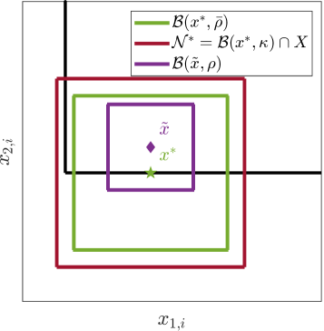
(a) Illustration for some $i\in{\mathcal{I}}_{+0}(x^{*})$

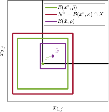
(b) Illustration for some $j\in{\mathcal{I}}_{00}(x^{*})$

Figure 5: Illustration of the argument used the proof of Theorem 4.1.

We apply this result now to Algorithm 2.

Corollary 4.1

Let Assumptions 4.1-4.4 hold. Let $x^{*}(\tau)$ be a stationary point of $\mathrm{Reg}(\tau)$ for some $\tau>0$. There exist positive constants $\bar{\tau}$, $\kappa$ such that for any: $\tau\in\left(0,\bar{\tau}\right]$ and $\rho\in[\sqrt{\tau},\kappa]$ the $\mathrm{LPEC}(x^{*}(\tau),\rho)$ in (13) is feasible. Moreover, for any feasible point $d$ of this LPEC, it follows that $\mathrm{BNLP}({\mathcal{I}}_{1}(x^{*}(\tau)+d),{\mathcal{I}}_{2}(x^{*}(\tau)+d))$ is feasible as well.

Proof. First, regard the case when $x^{*}(\tau)\in\Omega$, for some $\bar{\tau}\geq\tau>0$. The $\mathrm{LPEC}(x^{*}(\tau),\rho)$ is always feasible for this point and let $d$ be an element of its feasible set. Now for $\kappa=\bar{\rho}$ and all $\rho\in(0,\kappa)$, according to Lemma 3.2 all $\mathrm{BNLP}({\mathcal{I}}_{1}(x^{*}(\tau)+d),{\mathcal{I}}_{2}(x^{*}(\tau)+d))$ are feasible.

Second, for $x^{*}(\tau)\notin\Omega$ set $\tilde{x}=x^{*}(\bar{\tau})$ and apply Theorem 4.1. Since $x^{*}(\bar{\tau})$ is a stationary point of $\mathrm{Reg}(\bar{\tau})$, it holds that $c(x^{*}(\bar{\tau}))\geq 0$, i.e., $h_{c}(\tilde{x})=0$. Moreover, form $x_{1,i}x_{2,i}\leq\tau,\ \forall i\in\{1,\ldots,m\}$, it follows that $h(\tilde{x})\leq\sqrt{\bar{\tau}}=\delta$. Hence, for a sufficiently small $\delta=\bar{\tau}$ and every $0<\tau\leq\bar{\tau}$ the interval in (37) is nonempty and we can apply Theorem 4.1.

∎

Remarkably, the LPEC in the regularization-based Phase I does not even need to be solved for local optimality. It is sufficient to find a feasible point of the LPEC to identify a feasible BNLP. Now we have all the ingredients to state our main convergence result.

Theorem 4.2

Regard the MPEC (1) and suppose that Assumptions 4.1-4.4 hold. Then MPECopt given in Algorithm 3, with a sufficiently large finite number of iterations $N^{\mathrm{out}}$ and $N^{\mathrm{in}}$, with a Phase I from Section 3.3 has one of the following mutually exclusive outcomes:

1. It concludes that the MPEC (1) is locally infeasible.

2. It computes a point $x^{*}$ that is B-stationary for the MPEC (1) in a finite number of iterations.

Proof. We discuss Phase I first. Consider Algorithm 2. It follows from Lemma 3.5 that if $\mathrm{Reg}(\tau)$ is locally infeasible, then so is the MPEC  (1). On the other hand, if the MPEC is feasible, then it follows from Theorem 4.1 that Algorithm 2 will eventually find a feasible point $x^{0}$. Similarly, it follows from the discussion in Section 3.3.2, by solving the $\ell_{1}$ or $\ell_{\infty}$ reformulation of (25), local infeasibility is certified or a feasible point $x^{0}$ is found. This completes the proof for the first outcome.

Next, given a feasible point $x^{0}$, we show the finite termination of the Algorithm 3. Consider some iterate $x^{k}$, which is a stationary point of some $\mathrm{BNLP}({\mathcal{I}}_{1}(x^{k}),{\mathcal{I}}_{2}(x^{k}))$, and a $\rho^{k,l}>0$. If $d^{k,l}=0$ is a local minimizer of $\mathrm{LPEC}(x^{k},\rho^{k,l})$, then a B-stationary point is found and the algorithm terminates. Similarly, if ${\mathcal{I}}_{00}(x^{k})$ is empty, then $x^{k}$ is B-stationary. Otherwise, the $\mathrm{BNLP}({\mathcal{I}}_{1}(x^{k}+d^{k,l}),{\mathcal{I}}_{2}(x^{k}+d^{k,l}))$ is solved for $x^{k,l}$. If $f(x^{k,l})<f(x^{k})$ the step is accepted and $x^{k+1}=x^{k,l}$. If not, the radius of the trust region is reduced.

Now by Lemma 3.1 for a sufficiently small $\rho^{k,l}$ the full (13) and reduced LPECs (12) have the same set of local minimizers. Next, it follows from Lemma 3.2 that the point $x^{k}$ is feasible for any $\mathrm{BNLP}({\mathcal{I}}_{1}(x^{k}+d^{k,l}),{\mathcal{I}}_{2}(x^{k}+d^{k,l}))$. It follows from the equation (1) that a local minimizer of an LPEC is also a local minimizer for all branch LPs. Consider the $\mathrm{BNLP}({\mathcal{I}}_{1}(x^{k}+d^{k,l}),{\mathcal{I}}_{2}(x^{k}+d^{k,l}))$ and its corresponding branch LP, whose solution is $d^{k,l}\neq 0$. This means that $x^{k}$, which is feasible for $\mathrm{BNLP}({\mathcal{I}}_{1}(x^{k}+d^{k,l}),{\mathcal{I}}_{2}(x^{k}+d^{k,l}))$, is not a stationary point of this NLP, and according to the Assumption 4.1, the NLP solver will return a point with a lower objective value. From this analysis, we conclude that if $d^{k,l}\neq 0$ is a local minimizer of $\mathrm{LPEC}(x^{k},\rho^{k,l})$, then an acceptable step will be computed for a sufficiently small $\rho^{k,l}>0$.

This procedure generates a sequence of $\Delta f^{k}=f^{k}-f^{k+1}>0$. However, this sequence is also finite because the number of possible BNLPs is finite, and $\Omega$ is compact. Consider the last point $x^{K}$ in this sequence, found in a finite number of steps. Because no $\mathrm{BNLP}({\mathcal{I}}_{1}(x^{K}),{\mathcal{I}}_{2}(x^{K}))$ can produce a better objective, we conclude from Eq. (10) that $x^{K}$ stationary for all these BNLP, hence it is B-stationary for the MPEC (1). This concludes the proof. ∎

5 Numerical results

In this section, we extensively compare several MPECopt variants to some of the most successful regularization and penalty-based methods on two distinct nonlinear MPEC benchmarks.

5.1 Implementation

In our implementation and experiments, we treat MPECs more general than (1), given in the form of:

$$\underset{x\in{\mathbb{R}}^{n}}{\mathrm{min}}\;\quad f(x)$$ (38a)

s.t. $$c^{\mathrm{lb}}\leq c(x)\leq c^{\mathrm{ub}},$$ (38b)

$$x^{\mathrm{lb}}\leq x\leq x^{\mathrm{ub}},$$ (38c)

$$0\leq g(x)\perp h(x)\geq 0,$$ (38d)

where $c^{\mathrm{lb}},c^{\mathrm{ub}}\in{\mathbb{R}}^{n_{c}}$ are lower and upper bounds of $c(x)$ with $c^{\mathrm{ub}}_{i}\geq c^{\mathrm{lb}}_{i},\ \forall i\in\{1,\ldots,n_{c}\}$. Equality constraints are imposed by settings $c^{\mathrm{ub}}_{i}=c^{\mathrm{lb}}_{i}$. The vectors $x^{\mathrm{lb}},x^{\mathrm{ub}}\in{\mathbb{R}}^{n}$ are lower and upper bounds on $x$. If there is no lower or upper bound on some $x_{i}$ or $c_{i}(x)$, then we set the respective value on $-\texttt{inf}$ or inf. The nonlinear functions $g:{\mathbb{R}}^{n}\to{\mathbb{R}}^{m}$ and $h:{\mathbb{R}}^{n}\to{\mathbb{R}}^{m}$ are assumed to be twice continuously differentiable and model the complementarity constraint functions. They may simply select some components of $x\in{\mathbb{R}}^{n}$, i.e., $g(x)=x_{1}$ and $h(x)=x_{2}$. If they are more complicated, this is automatically detected and the nonlinear constraints are replaced by slack variables $x_{1}$ and $x_{2}$, i.e., (38d) is replaced by:

$$x_{1}-g(x)=0,$$

$$x_{2}-h(x)=0,$$

$$0\leq x_{1}\perp x_{2}\geq 0.$$

To solve the NLPs arising in MPECopt we use the IPOPT solver Waechter2006 . For better performance, we change some of the default options by setting the tolerance to $\texttt{tol}=10^{-12}$ (default is $10^{-8}$), $\texttt{acceptable\_tol}=10^{-9}$ (default is $10^{-6}$), and $\texttt{warm\_start\_init\_point}=\texttt{'yes'}$. Moreover, we change the barrier parameter strategy by setting: mu_strategy = ’adaptive’ and mu_oracle = ’quality-function’, cf. Nocedal2009 . In all experiments, we use MA27 Duff1982 from the HSL library HSL as the linear solver in IPOPT. The same settings are used for all methods and NLP solutions in the following experiments.

All problems are formulated in the symbolic framework of CasADi Andersson2019 via its Matlab interface. CasADi provides the first and second-order derivatives for all problem functions via its automatic differentiation and has an interface for calling IPOPT.

We use two different ways to solve the LPECs. First, we use the MILP formulation in (21) and solve it with the commercial solver Gurobi Gurobi or the open-source solver HiGHS Huangfu2018 . In our experiments, we used Matlab R2024a, where the HiGHS solver can be directly called from Matlab via the intlinprog function. For the MILPs, we set the maximum number of nodes in the branch and bound algorithm to 500 and the maximum computation time to 5 minutes. The tolerance for the LP solves in both MILP solvers is set to $10^{-9}$ (default is $10^{-6}$). Second, as LPECs are a special case of MPECs, we solve them via the homotopy regularization and penalty-based methods described below. The homotopy terminates if the solver reports local infeasibility or if a complementarity residual of $\|\mathrm{diag}(x_{1})x_{2}\|_{\infty}$ is below $10^{-9}$. The subproblems are solved with IPOPT.

For comparisons, we also implement the regularization and penalty-based methods from Section 2.2. Thereby, an adaptation of Reg($\tau$) and Pen($\tau$) to the form of  (38) are solved in a homotopy loop with a decreasing parameter $\tau$. We initialize $\tau^{0}=1$ and update it iteratively using the rule $\tau^{k}=0.1\tau^{k-1}$. The loop terminates if either: the NLP solution is feasible and the complementarity tolerance $h_{\perp}(x)$ is below $10^{-9}$; an NLP is locally infeasible; or a maximum number of $15$ iterations is reached. A homotopy loop is declared successful if it finds a stationary point. Recall that within the homotopy approach, unless the identified point is S-stationary, it remains unclear whether it is also B-stationary.

Our implementation of MPECopt is open-source and available at https://github.com/nosnoc/mpecopt. The repository contains several tutorial examples and the two benchmarks below.

5.2 Results on MacMPEC benchmark

We explore several algorithmic options of MPECopt on the MacMPEC benchmark set Leyffer2000 . The MacMPEC problem set is available in the form of a package of AMPL .mod and .dat files from wiki.mcs.anl.gov/leyffer/index.php/MacMPEC. We consider in total 191 problems. They are translated into the CasADi symbolic framework and are available in https://github.com/nosnoc/mpecopt/benchmarks/macmpec.

5.2.1 Comparison of different Phase I algorithms

In our first experiment, we compare several Phase I algorithms discussed in Section 3.3. In particular, we examine the following five versions:

1. Algorithm 2 with Reg($\tau$) and LPEC solves, $\rho_{I}=10^{-1}$ – Reg-LPEC.

2. Algorithm 2 with Reg($\tau$) and simple projection in (24) – Reg-Simple.

3. Algorithm 2 with $\ell_{1}$ reformulation of Pen($\tau$) and LPEC solves, $\rho_{I}=10^{-1}$ – Pen-$\ell_{1}$-LPEC.

4. The $\ell_{1}$ reformulation of (25) via Algorithm 3, $\rho^{0}=10^{0}$ – Feasibility-$\ell_{1}$.

5. The $\ell_{\infty}$ reformulation of (25) via Algorithm 3, $\rho^{0}=10^{0}$ – Feasibility-$\ell_{\infty}$.

Algorithm 2 with an $\ell_{\infty}$, instead of $\ell_{1}$ reformulation, achieves similar results as the $\ell_{1}$-approach, while being only slightly slower. We omit it from the plots for the sake of better readability. For all versions, we tried several initial trust region radii with smaller and larger values than in the list above. For the sake of brevity, we picked for each variant the best value and report only these results here. The initial trust region did not have much influence on the regularization-based methods within Algorithm 2, and the feasibility formulation (25) had slightly higher success rates with a larger value of the initial radius. In this experiment, Gurobi is used for solving LPECs by rewriting them into MILPs (21).

Results of the experiments are given in the Dolan-Moré absolute and relative performance profiles Dolan2002 . Phase I is declared as successful if it finds a feasible point $x^{0}\in\Omega$. The results for the different Phase I algorithms are given in Fig. 6.

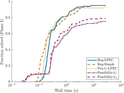
(a) Absolute timings.

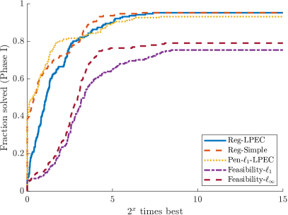
(b) Relative timings.

Figure 6: Evaluating different Phase I algorithms in MPECopt on the MacMPEC test set.

Overall, Reg-LPEC and Reg-Simple are the most successful approaches with a success rate of 95.29%, but they are not always the fastest. The simple projection, Reg-Simple, is mostly very effective for easy MPECs where there are no biactive constraints, as it quickly finds a feasible BNLP and does not require LPEC solves. However, it requires significantly more NLP solves on some examples, independent of the number of biactive constraint at the solution, and requires many NLP solves until $\tau$ becomes very small, which is needed to obtain a valid active set estimate via (24). In the worst case, on several problem instances such as pack-comp1-8, pack-comp1c-8, pack-comp1p-8, it requires 20 NLP solver calls, whereas solves Reg-LPEC require at most 8 NLP solves to compute a B-stationary point. In such cases, Reg-LPEC is faster, as it can be seen in Fig. 6. Pen-$\ell_{1}$-LPEC is often the fastest approach but has a lower success rate with 93.19%. The reason is that penalty strategies are in general faster than the regularization-based approach, but have a lower success rate in finding any stationary point of an MPEC. This is consistent with the overall results for these two strategies, reported in Fig. 10. However, even to Pen-$\ell_{1}$-LPEC is relatively the fastest, in Fig. 6a it can be seen that in absolute terms it is not significantly faster.

The feasibility-based methods Feasibility-$\ell_{\infty}$ and Feasibility-$\ell_{1}$ are in this benchmark less competitive than Algorithm 2, with success rates of 79.05% and 75.39%, respectively. In all other cases when they fail, a B-stationary point of  (25) with a nonzero residual is found.

Another advantage of Algorithm 2 over the feasibility approach is that they already take the objective of (1) into account. Therefore, the first feasible BNLP found Algorithm 2 and its solution $x^{0}$ may already yield a B-stationary point of the MPEC. In such cases, the first LPEC solve in Algorithm 3 only needs to verify B-stationarity. For Reg-LPEC this happens in 56.02%, for Reg-Simple in 74.34% and Pen-$\ell_{\infty}$-LPEC in 16.23% of the overall successful cases. In other words, when the regularization-based method is successful in finding B-stationary points, MPECopt inherits its efficacy, and Phase II immediately certifies the success. Moreover, an LPEC can often identify a feasible BNLP even for larger values of $\tau$. This implies a smaller number of total NLP solves in MPECopt compared to a regularization-based method, which we discuss in more detail in Section 5.2.3.

In conclusion, Reg-LPEC is the most successful Phase I approach and our default option for all other experiments below. As it can be seen in the absolute timing in Fig. 6a it is only slightly slower than Reg-Simple on easier MPECs, but manages to find reliably a feasible point in most of the cases. Recall that, although Reg-Simple does not require solving LPECs in Phase I, it still needs to solve LPECs in Phase II to verify B-stationarity or to determine a new BNLP.

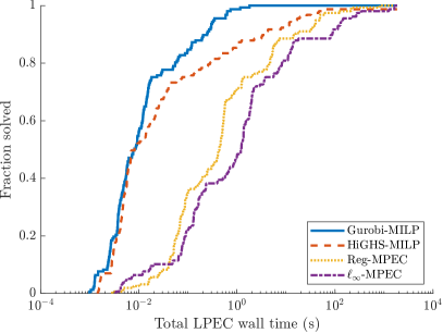
(a) Absolute timings.

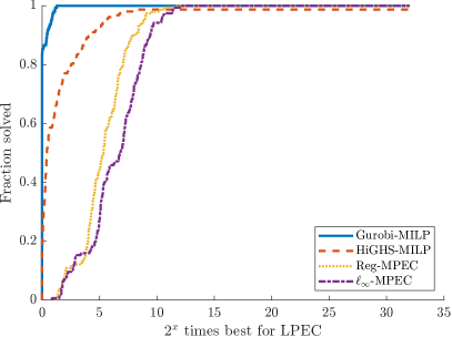
(b) Relative timings.

Figure 7: Evaluating different LPEC algorithms in MPECopt on the MacMPEC test set.

5.2.2 Comparison of different LPEC solvers

In our next experiment, we compare different LPEC solution strategies. In all experiments, we use the regularization-based Phase I Reg-LPEC, but we use different solvers for solving the LPECs in both phases. For the comparison, we consider four distinct variants where the LPEC is solved via

1. the MILP reformulation  (21) with Gurobi, and $\rho_{I}=10^{-1}$ in Phase I – Gurobi-MILP.

2. the MILP reformulation  (21) with HiGHS, and $\rho_{I}=10^{-3}$ in Phase I – HiGHS-MILP.

3. Generic MPEC with regularization-based reformulation Reg($\tau$) – Reg-MPEC.

4. Generic MPEC with $\ell_{1}$-penalty reformulation Pen($\tau$) – $\ell_{\infty}$-MPEC.

The HiGHS solver performs significantly better if the trust region in the LPEC is smaller. For this reason, we set in Phase I for this solver $\rho_{I}=10^{-3}$. Gurobi is less sensitive to these changes and has similar performance for larger and smaller values of $\rho_{I}$. We also conducted experiments using the $\ell_{\infty}$-penalty method, which produced results similar to those of the $\ell_{1}$-penalty method. To improve readability, we have omitted the $\ell_{\infty}$-penalty results from the plots blow.

We solve all problems in MacMPEC with the four different LPEC solution strategies. Thereby, we compare the total cumulative computation times spent for solving all LPECs in each MPEC instance of MacMPEC. In 34 of the 191 problems, after the first NLP is solved, either the MPEC is already solved or found to be locally infeasible. We exclude these from the plots, as the effective LPEC wall time in these 34 problems is zero. The remaining 157 problems are successfully solved by all approaches, except for HiGHS-MILP, which does not solve LPECs appearing in the problems siouxfls and siouxfls1.

Fig. 7 shows the absolute and relative performance profile with the total cumulative LPEC solution times. It can be seen that MILP strategies significantly outperform the regularization and penalty methods in terms of computation time.

This large difference has several causes. The MILP methods solve the LPEC to global optimality (which is sufficient for verifying B-stationary), whereas the other can compute only a stationary point (which may not even be a local minimum or B-stationary point of the LPEC). Consequently, LPEC solved by regularization-based methods tend to be more often locally infeasible in Phase I or need to solve more LPECs until a B-stationary point is verified in Phase II. To have a more fair comparison, in addition to the cumulative times, in Fig. 8 we show the maximum LPEC computation time in every of the 157 MPEC instances. Even there, we see that the MILP-based methods are up to two orders of magnitude faster than regularization-based methods for LPECs on the MacMPEC test set. This empirically confirms the arguments made in Section 3.2.2 on efficient solving LPECs as MILPs. Moreover, we observed often that, when the solution is S-stationary, the MILP is solved after one LP solve, which complies with the result of Lemma 3.3.

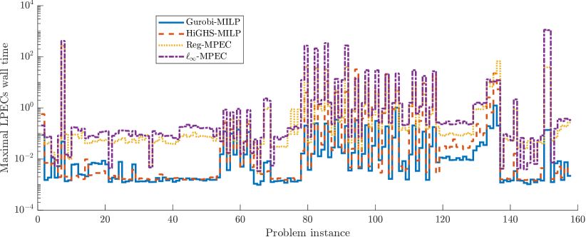
Figure 8: Maximal solution times for different LPEC algorithms in MPECopt on the MacMPEC test set.

Finally, we compare the cumulative NLP and LPEC computation times in every MPECopt solver call on every MacMPEC problem. The results are reported in Fig. 9, where the diagonal line means equal time spent on NLP and LPEC solving. We see that for the MILP methods, most dots are far below the diagonal, which means that a smaller fraction of the total computation time is spent on solving the LPECs, and the expensive part is solving the BNLPs. On the other hand, in the regularization-based methods, the dots cluster around and above the diagonal, meaning that the total computational burden is almost equally spread on solving NLPs and LPECs. In particular, the cumulative NLP time is smaller than the cumulative LPEC time in 0% of cases for Gurobi-MILP, 20% for HiGHS-MILP, 87.26 % for Reg-MPEC, and 85.99 % for $\ell_{\infty}$-MPEC. The MILP solvers, especially HiGHS profit from smaller initial true region radii in Phase I. However, the smaller $\rho_{I}$ the more NLPs in Phase I must be solved until a feasible LPEC is found, which shifts the computational load more to the NLP side.

To conclude, our experiments on MacMPEC confirm that solving LPECs via MILPs can be done very efficiently in practice, both with commercial (Gurobi) and open-source (HiGHS) solvers. Remarkably, in this benchmark, the MILP approaches are often orders of magnitude faster than the integer-free regularization-based methods for solving LPECs.

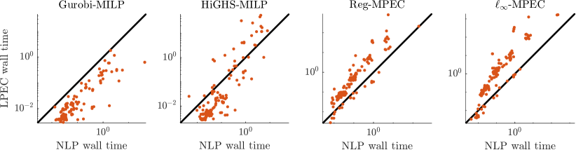
Figure 9: Comparison of total NLP and LPEC computation times on the MacMPEC.

5.2.3 Comparison of MPECopt to regularization-based methods

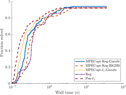
(a) Absolute timings.

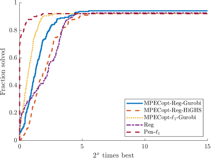
(b) Relative timings.

Figure 10: Evaluating different MPEC solution methods on the MacMPEC test set in terms of finding a stationary point.

Next, we compare MPECopt to the regularization and penalty-based solution methods from Section 2.2. For Phase I of MPECopt, we use again Reg-LPEC, which had the highest success rate in experiments from Section 5.2.1. In the following experiment, we compare in total five algorithms:

1. MPECopt, with regularization-based Phase I, and Gurobi as LPEC solver – MPECopt-Reg-Gurobi.

2. MPECopt, with $\ell_{1}$-penalty-based Phase I, and Gurobi as LPEC solver – MPECopt-$\ell_{1}$-Gurobi.

3. MPECopt, with regularization-based Phase I, and HiGHS as LPEC solver – MPECopt-HiGHS.

4. Regularization-based method, that solve Reg($\tau$) in a homotopy loop– Reg.

5. $\ell_{1}$-penalty-based method, that solve an $\ell_{1}$ reformulation of Pen($\tau$) in a homotopy loop – Pen-$\ell_{1}$.

We also tried the $\ell_{\infty}$ penalty method, which similar computation time as $\ell_{1}$, but a slightly lower success rate. Therefore, for better readability, we omit it from the plots. Moreover, MPECopt with the simple projection strategy, i.e., Reg-Simple from Section 5.2.1 performs similar to MPECopt-Reg-Gurobi, and we omit it as well for better readability of the plots.

We first compare the success rate and computations point for finding a stationary point. Note that, if MPECopt is successful, it always returns a B-stationary point, whereas for the other methods, we can only know that it is a B-stationary point if it is also S-stationary. Fig. 10 reports the absolute and relative performance profiles for this experiment.

We can see that MPECopt-Reg-Gurobi achieves in total the highest success rate of 94.24%. It is faster and more successful than its counterpart Reg (92.67%). The $\ell_{1}$ penalty method is faster than MPECopt-Reg-Gurobi, but with a smaller success rate of 92.14%. On the other hand, MPECopt-$\ell_{1}$-Gurobi is only slightly slower than Pen-$\ell_{1}$ and achieves the same success rate. MPECopt-Reg-HiGHS is slightly slower than MPECopt-Reg-Gurobi, and has a lower success rate of 92.67%, because HiGHS fails to solve LPECs in Phase II in the problems incid-set-32, incid-set2-32 and incid-setc-32. The difference in computation times is consistent with Fig. 9.

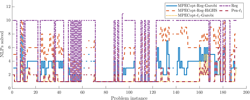
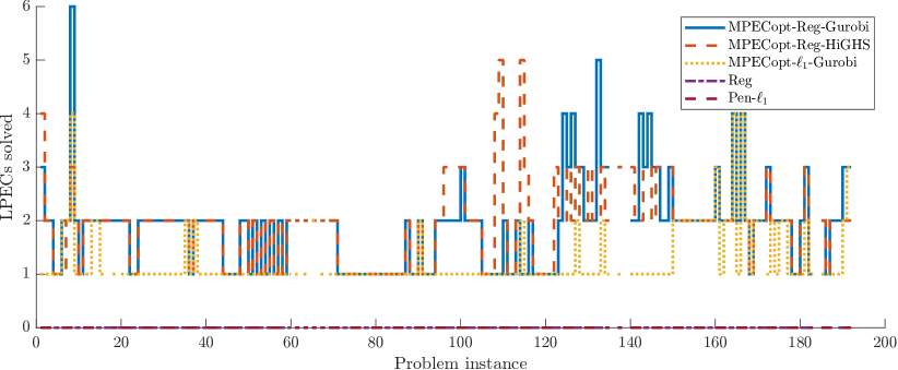
Figure 11: Number of NLPs (top plot) and NLPs (bottom plots) solved in MacMPEC on all problem instances.

The MPECopt method inheres the efficacy of the standard methods used in Phase I, but can often be even faster as it requires fewer NLP solves. The reason is that already for a moderate value of $\tau$, the LPEC can identify a feasible BNLP in Phase I. Figure 11 shows the number of NLPs and LPECs solved in every problem instance. The plot does not include the NLP and LPEC solved used to determine the type of stationary points for Reg and Pen-$\ell_{1}$ in the next section. We observe that MPECopt-Reg-Gurobi and MPECopt-Reg-HiGHS consistently solve a smaller number of NLPs than their counterpart Reg. Similar holds for MPECopt-$\ell_{1}$-Gurobi and Pen-$\ell_{1}$. Moreover, MPECopt requires in most cases only a few LPEC solutions. In many cases, it is only two, one in Phase I to identify a feasible BNLP, and one in Phase II to verify B-stationarity.

All methods are quite fast on easy problems where there are no biactive constraints, and often a single NLP solve is sufficient to find a solution. Approximately more than two-thirds of solutions found by any of the algorithms have an empty biactive set.

5.2.4 Comparison of stationary points

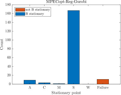
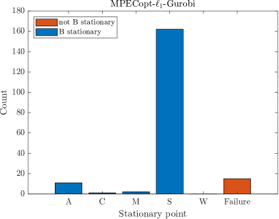
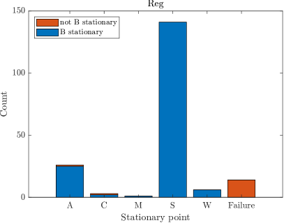
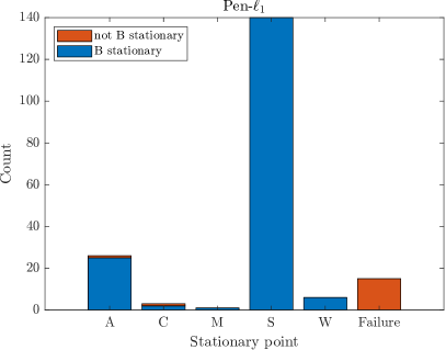
Figure 12: Distribution of stationary points on MacMPEC for different solution methods. Failure counts the number of infeasible problems.

Now we look at the distribution of stationary point types found by the algorithms compared in the previous section. We also check are these points B-stationary. To determine the type of stationary point from Definition 2.3 we must solve the TNLP (9), which requires a correct identification of the active sets ${\mathcal{I}}_{+0},{\mathcal{I}}_{0+}$ and ${\mathcal{I}}_{00}$. MPECopt is an active set method where the complementarity constraints are usually satisfied exactly or close to machine precision, making it easy to find the active sets for the TNLP. On the other hand, Reg, and Pen-$\ell_{1}$ rarely have a complementarity residual $h_{\perp}(x)$ much smaller than the prescribed tolerance of $10^{-9}$, making an active set identification more difficult. We take an iterative procedure, and identify the active set via Eq. (19), with $\epsilon=10^{-6}$. To minimize the possibility of wrong conclusions, we implement several safeguards. We denote the solution computed via Reg or Pen-$\ell_{1}$ by $x^{*}$, and the corresponding TNLP solution by $x^{\mathrm{tnlp}}$. We declare the active set to be correctly identified if $\|x^{*}-x^{\mathrm{tnlp}}\|\leq 10^{-7}$. If this is not satisfied we reduce $\epsilon$ by a factor of 10 and repeat the procedure. Once $\|x^{*}-x^{\mathrm{tnlp}}\|\leq 10^{-7}$ is true or a maximum number of 5 attempts is exceeded, we compute the multipliers in the TNLP and classify the stationary point. To verify B-stationarity, we take several steps. First, we use the point $x^{\mathrm{tnlp}}$ and construct an ${\mathrm{LPEC}}(x^{\mathrm{tnlp}},\rho)$ with $\rho=10^{-3}$. If the objective of this LPEC is below $\texttt{tol}_{\mathrm{B}}=10^{-8}$, then we declare a $x^{*}$ to be B-stationary. If this is not the case, we take up to three more LPEC solve attempts while reducing $\rho$ by a factor of 10. The minimal value is $\rho=10^{-6}$, which is the minimal allowed trust region radius in MPECopt. This delivers a valid certificate in most cases. To have more robustness to wrong active set identification, if this does not verify B-stationarity, we repeat the same but now with $x^{*}$ as linearization point ${\mathrm{LPEC}}(x^{*},\rho)$. Finally, if this also fails, we look at the objective $f(x^{*})$ and the objective computed by MPECopt for the same problem, which is denoted by $f(\hat{x})$. If the relative difference satisfies $\frac{|f(x^{*})-f(\hat{x})|}{|f(\hat{x})|+10^{-16}}<10^{-3}$, then we declare $x^{*}$ to be B-stationary, if $\hat{x}$ is B-stationary. If the difference between the objective is larger, and the LPECs find a descent direction, the point $x^{*}$ is declared to be not B-stationary.

Figure 12 plots the distribution of the stationary points for all solvers except MPECopt-Reg-HiGHS, which is the same as MPECopt-Reg-Gurobi (except on the problems that were not solved). S stationary points dominate the overall picture, as two-thirds of problems have no biactive constraints. MPECopt always converges to a B-stationary point by construction. Using the above-described procedure for identifying stationary points, Reg and Pen-$\ell_{1}$ fail only in two cases to find a B-stationary point. This happens on the problems ralph2 (A-stationary) and scholtes4 (C-stationary). MPECopt computes in both cases a B-stationary point with the objective value of $10^{-12}$, whereas Reg computes objectives of $0.6325\cdot 10^{-4}$, which is too far away from the B-stationary point. Similar results are obtained with Pen-$\ell_{1}$. This can be improved by reducing significantly the complementarity tolerance in the homotopy loop, e.g. $10^{-14}$ instead of $10^{-9}$. However, this makes Reg and Pen-$\ell_{1}$ significantly slower, and fail more often on other problems.

In summary, we can say that all methods, sometimes with some tuning, can successfully compute B-stationary points on MacMPEC (and MPECopt directly certifies this). To get a broader perspective, we run another benchmark in the next section.

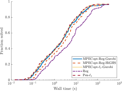
(a) Absolute timings.

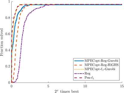
(b) Relative timings.

Figure 13: Evaluating different MPEC solution methods on the synthetic test set in terms of finding a stationary point.

5.3 Synthetic nonlinear MPEC benchmark

Many problems in MacMPEC are relatively small or easy to solve with any of the examined algorithms. Moreover, two-thirds of problems have an empty biactive and very few non-S stationary points, making the verification of B-stationarity often trivial. To compare MPECopt further, we consider a synthetic nonlinear MPEC benchmark, where the solutions have many biactive constraints. Details on the problem generation are described in the Appendix A, and an open-source implementation can be found at https://github.com/nosnoc/mpecopt/benchmarks/nonlinear_mpec.

For the sake of brevity, we only do here the same experiments as in Sections 5.2.3 and 5.2.4. All others can be recreated by running the code in https://github.com/nosnoc/mpecopt/benchmarks/nonlinear_mpec. Notably, in contrast to MacMPEC, in the case of Phase I algorithms, Reg-Simple is slower and less successful than Reg-LPEC on this test set. Moreover, the feasibility $\ell_{1}$ and $\ell_{\infty}$ become more competitive and are closer to Reg-Simple. Overall, Reg-LPEC and $\ell_{1}$-LPEC are still the fastest and most successful Phase I strategies.

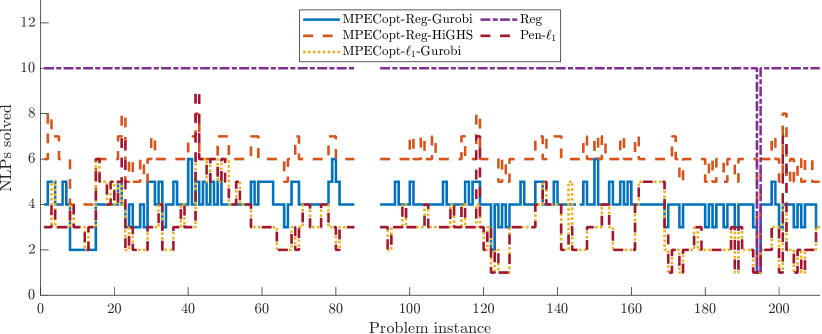
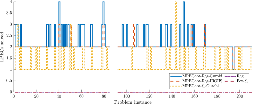
Figure 14: Number of NLPs (top plot) and NLPs (bottom plots) solved in the synthetic test set on all problem instances.

Fig. 13 shows the relative and absolute performance profiles, and Fig. 14 the total number of NLPs and LPECs solved on each problem instance. Simile to the results on MacMPEC (Fig. 10), we see that the MPECopt variants are the fastest and most successful algorithms, for the same reasons as in the previous experiments, i.e., a smaller number of total NLP solves is needed, see Fig. 14. Moreover, on this set, the differences in terms of computation times, between MPECOpt-Reg-Gurobi (96.16% success rate), MPECOpt-$\ell_{1}$-Gurobi (96.67% success rate), and Pen-$\ell_{1}$ (96.67% success rate) are less significant, wheres Reg (96.67% success rate) needs to solve more NLPs and is thus solver. MPECOpt-Reg-HiGHS (96.67% success rate) is slightly slower than MPECopt variants using Gurobi, but is still faster than Reg. In cases where they fail, all algorithms report to find a locally infeasible point. It can be seen in Fig. 14 that MPECopt variants solve fewer NLPs than Reg, whereas MPECOpt-$\ell_{1}$-Gurobi and Pen-$\ell_{1}$ usually require the same number of NLP solves. In most cases only one to two LPEC solves are needed, which do not add significantly to the overall computation time, cf. Fig. 13a.

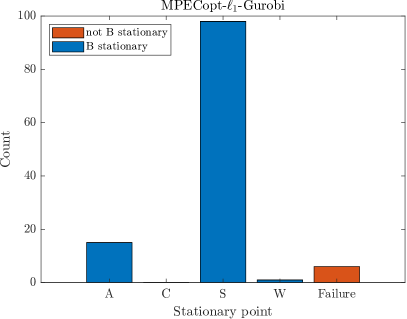
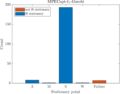
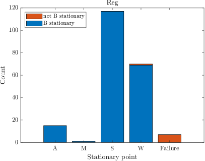
Figure 15: Distribution of stationary points on the synthetic test set for different solution methods. Failure counts the number of infeasible problems.

Next, we examine the different types of stationary points in Fig. 15. This problem set is more balanced, as only about a quarter of the problems have no biactive constraints. To determine the type of stationary point or to verify B-stationarity we use the same iterative procedure as in Section 5.2.4. Since there are many biactive constraints, and MPEC-LICQ is often violated, there are more non-S stationary points. In this set, Pen-$\ell_{1}$ manages to find in all cases B-stationary point, even though MPEC-LICQ is violated. To the best of our knowledge, currently existing theoretical results do not fully explain this. In four problems Reg finds W-stationary points that are not B-stationary. On the other hand, its MPECopt counterpart finds B-stationary points with a significantly better objective value in these cases. We remind the reader that verifying the B-stationarity of non-S-stationary points computed by Reg and Pen-$\ell_{1}$ usually requires solving several additional NLPs and LPECs in addition to the computations shown in Figures 13 and 14. Our experiments empirically confirm, that Reg sometimes does not converge to B-stationary points. However, this did not happen very often in all of our experiments.

6 Conclusions and summary

This paper introduced MPECopt, a numerical method for computing B-stationary points of mathematical programs with equilibrium constraints (MPECs). MPECopt operates in two phases. The first phase identifies a feasible point of the MPEC or certifies local infeasibility. The second phase iterates over feasible points to find a B-stationary point by solving a finite sequence of branch nonlinear programs (BNLPs) and linear programs with equilibrium constraints (LPECs). The LPEC is directly equivalent to the definition of B-stationarity.

We proposed two distinct strategies for Phase I. The first strategy leverages the effectiveness of existing regularization and penalty-based methods. The second approach involves solving a feasibility MPEC directly using the Phase II algorithm. The paper includes a detailed theoretical analysis of two LPEC subproblem formulations and provides a comprehensive convergence theory for MPECopt. In particular, Theorem  4.2 proves that the algorithm terminates after a finite number of iterations. All theoretical results are illustrated and motivated by a series of tutorial examples.

We argue that the nonconvex LPEC subproblems can be efficiently solved using mixed-integer linear programming (MILP) methods. On two moderate-size benchmark problem sets we demonstrate that this is indeed the case and that solving LPECs is not a computational bottleneck in practice. Interestingly, we prove that if a point is S-stationary, solving a single linear program (LP) is sufficient for solving the MILP reformulation of the LPEC constructed at this point. Another key finding, proven in Theorem 4.1, is that, given a point close enough to a feasible point of the MPEC, then just by finding a feasible point of an LPEC constructed at this point is sufficient for identifying a feasible BNLP. Moreover, the trust-region radius of the LPECs in Phase II can be arbitrarily small, leading to very tight relaxations and efficient solutions via MILP methods – often two order magnitudes faster than homotopy-based methods for LPECs.

In addition to the theoretical analysis, this paper is accompanied by an open-source implementation of MPECopt available at https://https://github.com/nosnoc/mpecopt, including the algorithmic variations discussed. The method is relatively easy to implement, benefiting from robust and mature NLP and MILP solvers. We tested MPECopt on two extensive numerical benchmarks: the MacMPEC set and a synthetic nonlinear MPEC test set, introduced in this paper. Numerical results confirm the efficacy of the proposed methods for finding B-stationary points. MPECopt is usually faster and more reliable than existing methods, requiring fewer NLP solves than existing homotopy-based methods.

An intriguing observation from the benchmarks is that regularization and penalty-based methods frequently identify B-stationary points that are not S-stationary. To our knowledge, the current convergence results for these methods do not explain this phenomenon. However, verifying this currently requires solving additional nonlinear programs and LPECs, whereas MPECopt inherently certifies B-stationarity as solving LPECs is integrated into the algorithm.

Finally, in this paper we assume that the BNLPs are solved to full convergence. A natural direction for future work would be to study inexact BNLP solutions while maintaining robust and fast convergence. This extension would likely require a more sophisticated globalization strategy, since most iterates would not be exactly feasible. However, Theorem 4.1 suggests that LPECs constructed near feasible points have similar properties to those constructed at feasible points. This insight should be exploited in the design of new numerical methods. From an implementation point of view, it would be interesting to test tailored LPEC methods Fang2010 ; Hu2012 ; JaraMoroni2020 ; JaraMoroni2018 within MPECopt.

Appendix A Generating a synthetic MPEC benchmark

In this section, we describe how we generate a random set of MPECs that are used in the numerical experiments of Section 5.3. The problem-generating function and code to reproduce the benchmark results is available at https://github.com/nosnoc/benchmarks/nonlinear_mpec_benchmark.

A summary of how the random MPECs are generated is given in Algorithm 4. Additionally, we describe how the problems are generated. First, we generate random LPECs as described in Hu2008 . They have the following form:

$$\underset{x_{0}\in{\mathbb{R}}^{p},x_{1}\in{\mathbb{R}}^{m}}{\min}\;\quad g_{0}^{\top}x_{0}+g_{1}^{\top}x_{1}$$ (39a)

s.t. $$Ax_{0}+Bx_{1}\geq a$$ (39b)

$$0\leq x_{1}\perp Mx_{0}+Nx_{1}+q\geq 0,$$ (39c)

where $g_{0}\in{\mathbb{R}}^{p}$, $g_{1}\in{\mathbb{R}}^{m}$ are the cost vectors. The inequality constraint data has the following dimensions $A\in{\mathbb{R}}^{n_{\mathrm{ineq}}\times p}$, $B\in{\mathbb{R}}^{n_{\mathrm{ineq}}\times m}$, $a\in{\mathbb{R}}^{n_{\mathrm{ineq}}}$. The dimensions of the data in left hand side of (39c) are $M\in{\mathbb{R}}^{m\times p}$, $N\in{\mathbb{R}}^{m\times m}$ and $q\in{\mathbb{R}}^{m}$. A pseudocode for the generation of these LPECs can be found in (JaraMoroni2020, , p. 22). We use the same description as a starting point but allow more flexibility in changing the problem data and dimensions.

To generate a nonlinear MPEC, we make the following modification to the LPEC (39). We replace the objective in (39a) by $f(x)=f^{\mathrm{nl}}(x_{0},x_{1})+\alpha g_{0}^{\top}x_{0}+\alpha g_{1}^{\top}x_{1}$, where $f^{\mathrm{nl}}(x_{0},x_{1})$ is a nonlinear objective test function from Andrei2008 . Let $c^{\mathrm{ineq}}(x)=Ax_{0}+Bx_{1}-a\geq 0$ define the inequality constraints. To introduce more nonlinearity, we consider a subset of inequality constraint indices, i.e., ${\mathcal{I}}^{\mathrm{ineq}}\subseteq\{1,\ldots,n_{\mathrm{ineq}}\}$. Next, all inequality constraints $c_{i}^{\mathrm{ineq}}(x)\geq 0$ with $i\in{\mathcal{I}}^{\mathrm{ineq}}$ are replaced by $c_{i}^{\mathrm{ineq}}(x)+c_{i}^{\mathrm{ineq}}(x)^{2}+c_{i}^{\mathrm{ineq}}(x)^{4}\geq 0$. Moreover, we duplicated a subset of the inequality constraints (both linear and nonlinear), with indices $i\in{\mathcal{I}}^{\mathrm{d}}\subseteq\{1,\ldots,n_{\mathrm{ineq}}\}$. This makes the MPEC more degenerate as it increases the probability of violating MPEC-LICQ if inequality constraints are active. Next, we define equality constraints by introducing a slack variable $x_{2}\in{\mathbb{R}}^{m}$ for the left hand side in  (39c), which reads as $c^{\mathrm{eq}}(x)=x_{2}-Mx_{0}+Nx_{1}+q$. Analogously to the inequality constraints, we replace some constraints by $c^{\mathrm{eq}}_{i}(x)=0$ by $c^{\mathrm{eq}}_{i}(x)+c^{\mathrm{eq}}_{i}(x)^{2}+c^{\mathrm{eq}}_{i}(x)^{4}=0,i\in{\mathcal{I}}^{\mathrm{eq}}\subseteq\{1,\ldots,m\}$. Moreover, we add upper bounds $x^{\mathrm{ub}}_{0},x^{\mathrm{ub}}_{1}$ on $x_{0}$ and $x_{1}$.

The full pseudocode for generating a single problem instance is given in Algorithm 4. Thereby, $\mathcal{N}(\mu,\sigma^{2})$ denotes the normal distribution with $\mu$ mean and $\sigma$ standard deviation. The elements of $\mathcal{U}_{n}(a,b)$ are $n$ dimensional vectors whose elements are drawn from a uniform distribution on the interval $[a,b]$. Similarly, the elements of $\mathcal{U}_{n\times k}(a,b,s)$ are $n\times k$ matrices whose elements take values from a uniform distribution on $[a,b]$. The scalar $s\in\left(0,1\right]$ is the density of this random matrix, which is defined as the ratio between the number of nonzero elements and the total number of elements of this matrix.

Algorithm 4 Random MPEC generator

1:Input: Dimensions: $p,m,n_{\mathrm{ineq}}$; nonlinear objective function: $f^{\mathrm{nl}}(x_{0},x_{1})$; cost weight: $\alpha\geq 0$; proportion of nonlinear equality and inequality constraints: $s^{\mathrm{eq}},s^{\mathrm{ineq}}\in[0,1]$; proportion of duplicated inequality constraints $s^{d}\in[0,1]$.

2:Initial guess and upper bounds.

3:Generate initial guess $x_{0}^{0}\sim\mathcal{N}_{p}(0,1)$ and $x_{0}^{0}=|x_{0}^{0}|$.

4:Generate initial guess $x_{1}^{0}\sim\mathcal{N}_{m}(0,1)$ and $x_{1}^{0}=\max(0,x_{1}^{0})$.

5:Generate upper bounds $x_{0}^{\mathrm{ub}}\sim\mathcal{U}_{p}(100,1000)$ and $x_{1}^{\mathrm{ub}}\sim\mathcal{U}_{m}(100,1000)$.

6:Equality constraints.

7:Choose density for the random matrices $s\sim\mathcal{U}_{1}(0.1,0.3)$.

8:Generate random integer number $r\sim\mathrm{round}(\mathcal{U}_{1}(1,m))$.

9:Generate matrix $E\sim\mathcal{U}_{r\times(n-r)}(2,3,s)$, vectors $d_{1}\sim\mathcal{U}_{r}(0,2)$, $d_{2}\sim\mathcal{U}_{m-r}(0,2)$, and let $D_{1}=\mathrm{diag}(d_{1})$, $D_{2}=\mathrm{diag}(d_{2})$, $M=\begin{bmatrix}D_{1}&E\\ -E^{\top}&D_{2}\end{bmatrix}$.

10:Generate matrix $N\sim\mathcal{U}_{m\times p}(-1,1,s)$ and vector $q\sim\mathcal{U}_{r}(-20,-10)$,

11:Define $c^{\mathrm{eq}}(x)=Mx_{1}+Nx_{0}+q-x_{2}=0$ and $x=(x_{0},x_{1},x_{2})\in{\mathbb{R}}^{n},n=p+2m$.

12:Pick a random subset ${\mathcal{I}}^{\mathrm{eq}}\subseteq\{1,\ldots,m\}$ with cardinality $|{\mathcal{I}}^{\mathrm{eq}}|=\mathrm{round}(s^{\mathrm{eq}}m)$.

13:Replace $c_{i}^{\mathrm{eq}}(x)=0$ by $c_{i}^{\mathrm{eq}}(x)+c_{i}^{\mathrm{eq}}(x)^{2}+c_{i}^{\mathrm{eq}}(x)^{4}=0$ for all $i\in{\mathcal{I}}^{\mathrm{eq}}$.

14:Inequality constraints

15:Generate $A\sim\mathcal{U}_{n_{\mathrm{ineq}}\times p}(0,1,s)$, $B=\mathcal{U}_{n_{\mathrm{ineq}}\times m}(0,1,s)$

16:Generate $a=Ax_{0}^{0}+Bx_{1}^{0}-|\epsilon|$, $\epsilon\in\mathcal{N}_{n_{\mathrm{ineq}}}(0,1)$.

17:Define inequality constraints $c^{\mathrm{ineq}}(x)=Ax_{0}+Bx_{1}-a\geq 0$.

18:Pick a random subset ${\mathcal{I}}^{\mathrm{ineq}}\subseteq\{1,\ldots,n_{\mathrm{ineq}}\}$ with cardinality $|{\mathcal{I}}^{\mathrm{ineq}}|=\mathrm{round}(s^{\mathrm{ineq}}n_{\mathrm{ineq}})$.

19:Replace $c_{i}^{\mathrm{ineq}}(x)\geq 0$ by $c_{i}^{\mathrm{ineq}}(x)+c_{i}^{\mathrm{ineq}}(x)^{2}+c_{i}^{\mathrm{ineq}}(x)^{4}=0$ for all $i\in{\mathcal{I}}^{\mathrm{ineq}}$.

20:Pick a random subset ${\mathcal{I}}^{\mathrm{d}}\subseteq\{1,\ldots,n_{\mathrm{ineq}}\}$ with cardinality $|{\mathcal{I}}^{\mathrm{d}}|=\mathrm{round}(s^{\mathrm{d}}n_{\mathrm{ineq}})$ and duplicate inequality constraints $c_{i}^{\mathrm{ineq}}(x)\geq 0$ for all $i\in{\mathcal{I}}^{\mathrm{d}}$.

21:Objective function.

22:Generate $g_{0}\in\mathcal{U}_{p}(0,1)$, $g_{1}\in\mathcal{U}_{m}(1,3)$.

23:Define objective function $f(x)=f(x_{0},x_{1})+\alpha g_{0}^{\top}x_{0}+\alpha g_{1}^{\top}x_{1}$.

Our implementation allows to replacement of any random scalar variable (e.g. density $s$) by fixed values. In the implementation, the ranges of values from where the random variables are drawn can also be adapted, but for ease of notation, we write in Algorithm 4 the values used in our experiments.

To generate a problem test set, we consider 30 objective functions. Two of them correspond to positive definite and indefinite quadratic objectives, of the form: $f(x)=(x_{0},x_{1})^{\top}H(x_{0},x_{1})+g^{\top}(x_{0},x_{1})$, where $H=0.5(\hat{H}^{\top}+\hat{H})$, $\hat{H}\sim\mathcal{U}_{(p+m)\times(p+m)}(0,1,s)$ and vector $g\sim\mathcal{U}_{p+m}(-10,10)$. Only in these two cases, we do not make the equality and inequality constraints nonlinear. For the other 28 functions, we use the following nonlinear test functions from Andrei2008 : Fletcher, Himmelblau, McCormick, Powell, Trigonometric, Rosenbrock, Raydan1, Raydan2, Diagonal3, Diagonal4, Diagonal5, Extended_Trigiaonal, Three_Exponential_Terms, Generalized_PSC1, Extended_PSC1, Fletcvb3, Bdqrtic, Tridia, EG2, Edensch, Indef, Cube, Bdexp, Genhumps, Arwhead, Quartc, Cosine, Sine. For every test function, we generate $7$ problem instances with different sizes, resulting in a total of $210$ MPECs. The dimensions of $p$ are unique random integers from the set $\{10,\ldots,300\}$, $p=m$ and $n_{\mathrm{ineq}}~\mathrm{round}(\mathcal{U}_{1}(0.1p,2p))$. The remaining parameters we use in Algorithm 4 are $\alpha=10$, $s^{\mathrm{eq}}=0.5$, $s^{\mathrm{ineq}}=0.5$, and $s^{d}=0.5$.

References

- [1] Wolfgang Achtziger and Christian Kanzow. Mathematical programs with vanishing constraints: optimality conditions and constraint qualifications. Mathematical Programming, 114:69–99, 2008.
- [2] Sebastian Albrecht and Michael Ulbrich. Mathematical programs with complementarity constraints in the context of inverse optimal control for locomotion. Optimization Methods and Software, 32(4):670–698, 2017.
- [3] J. A. E. Andersson, J. Gillis, G. Horn, J. B. Rawlings, and M. Diehl. CasADi – a software framework for nonlinear optimization and optimal control. Mathematical Programming Computation, 11(1):1–36, 2019.
- [4] Neculai Andrei. An unconstrained optimization test functions collection. Adv. Model. Optim, 10(1):147–161, 2008.
- [5] M. Anitescu. Global convergence of an elastic mode approach for a class of mathematical programs with complementarity constraints. SIAM Journal on Optimization, 16:120–145, 2005.
- [6] Mihai Anitescu. On using the elastic mode in nonlinear programming approaches to mathematical programs with complementarity constraints. SIAM Journal on Optimization, 15(4):1203–1236, 2005.
- [7] BT Baumrucker, Jeffrey G Renfro, and Lorenz T Biegler. Mpec problem formulations and solution strategies with chemical engineering applications. Computers & Chemical Engineering, 32(12):2903–2913, 2008.
- [8] Pietro Belotti, Christian Kirches, Sven Leyffer, Jeff Linderoth, James Luedtke, and Ashutosh Mahajan. Mixed-integer nonlinear optimization. Acta Numerica, 22:1–131, 2013.
- [9] Choong Ming Chin and Roger Fletcher. On the global convergence of an slp–filter algorithm that takes eqp steps. Mathematical Programming, 96:161–177, 2003.
- [10] Victor DeMiguel, Michael P Friedlander, Francisco J Nogales, and Stefan Scholtes. A two-sided relaxation scheme for mathematical programs with equilibrium constraints. SIAM Journal on Optimization, 16(2):587–609, 2005.
- [11] E. D. Dolan and J. J. Moré. Benchmarking optimization software with performance profiles. Math. Program., 91:201–213, 2002.
- [12] Iain S. Duff and John Ker Reid. MA27 – a set of fortran subroutines for solving sparse symmetric sets of linear equations. 1982.
- [13] F. Facchinei and J.-S. Pang. Finite-dimensional variational inequalities and complementarity problems, volume 1-2. Springer-Verlag, 2003.
- [14] Haw-ren Fang, Sven Leyffer, and Todd Munson. A pivoting algorithm for linear programming with linear complementarity constraints. Optimization Methods and Software, 27(1):89–114, 2012.
- [15] Michael L Flegel and Christian Kanzow. Abadie-type constraint qualification for mathematical programs with equilibrium constraints. Journal of Optimization Theory and Applications, 124(3):595–614, 2005.
- [16] Roger Fletcher and Sven Leyffer. Nonlinear programming without a penalty function. Mathematical Programming, 91:239–269, 2002.
- [17] Roger Fletcher, Sven Leyffer, and Philippe L Toint. On the global convergence of a filter–sqp algorithm. SIAM Journal on Optimization, 13(1):44–59, 2002.
- [18] Masao Fukushima and Paul Tseng. An implementable active-set algorithm for computing a b-stationary point of a mathematical program with linear complementarity constraints. SIAM Journal on Optimization, 12(3):724–739, 2002.
- [19] Jacques Gauvin. A necessary and sufficient regularity condition to have bounded multipliers in nonconvex programming. Mathematical Programming, 12(1):136–138, 1977.
- [20] Giovanni Giallombardo and Daniel Ralph. Multiplier convergence in trust-region methods with application to convergence of decomposition methods for mpecs. Mathematical Programming, 112(2):335–369, 2008.
- [21] P. Gill, W. Murray, and M. Saunders. SNOPT: An SQP algorithm for large-scale constrained optimization. SIAM Review, 47(1):99–131, 2005.
- [22] Lei Guo and Zhibin Deng. A new augmented lagrangian method for mpccs—theoretical and numerical comparison with existing augmented lagrangian methods. Mathematics of Operations Research, 47(2):1229–1246, 2022.
- [23] Gurobi Optimization, LLC. Gurobi Optimizer Reference Manual, 2022.
- [24] Lisa C Hegerhorst-Schultchen, Christian Kirches, and Marc Christian Steinbach. On the relation between mpecs and optimization problems in abs-normal form. Optimization Methods and Software, 35(3):560–575, 2020.
- [25] Tim Hoheisel, Christian Kanzow, and Alexandra Schwartz. Theoretical and numerical comparison of relaxation methods for mathematical programs with complementarity constraints. Mathematical Programming, 137(1):257–288, 2013.
- [26] HSL. A collection of Fortran codes for large scale scientific computation. http://www.hsl.rl.ac.uk, 2011.
- [27] Jing Hu, John E Mitchell, Jong-Shi Pang, Kristin P Bennett, and Gautam Kunapuli. On the global solution of linear programs with linear complementarity constraints. SIAM Journal on Optimization, 19(1):445–471, 2008.
- [28] Jing Hu, John E Mitchell, Jong-Shi Pang, and Bin Yu. On linear programs with linear complementarity constraints. Journal of Global Optimization, 53:29–51, 2012.
- [29] Qi Huangfu and JA Julian Hall. Parallelizing the dual revised simplex method. Mathematical Programming Computation, 10(1):119–142, 2018.
- [30] Alexey F Izmailov and Mikhail V Solodov. An active-set newton method for mathematical programs with complementarity constraints. SIAM Journal on Optimization, 19(3):1003–1027, 2008.
- [31] J Ye Jane. Necessary and sufficient optimality conditions for mathematical programs with equilibrium constraints. Journal of Mathematical Analysis and Applications, 307(1):350–369, 2005.
- [32] Francisco Jara-Moroni, John E Mitchell, Jong-Shi Pang, and Andreas Wächter. An enhanced logical benders approach for linear programs with complementarity constraints. Journal of Global Optimization, 77:687–714, 2020.
- [33] Francisco Jara-Moroni, Jong-Shi Pang, and Andreas Wächter. A study of the difference-of-convex approach for solving linear programs with complementarity constraints. Mathematical Programming, 169:221–254, 2018.
- [34] Houyuan Jiang and Daniel Ralph. Qpecgen, a matlab generator for mathematical programs with quadratic objectives and affine variational inequality constraints. Computational Optimization and Applications, 13:25–59, 1999.
- [35] Abdeslam Kadrani, Jean-Pierre Dussault, and Abdelhamid Benchakroun. A new regularization scheme for mathematical programs with complementarity constraints. SIAM Journal on Optimization, 20(1):78–103, 2009.
- [36] Christian Kanzow and Alexandra Schwartz. A new regularization method for mathematical programs with complementarity constraints with strong convergence properties. SIAM Journal on Optimization, 23(2):770–798, 2013.
- [37] Christian Kanzow and Alexandra Schwartz. The price of inexactness: convergence properties of relaxation methods for mathematical programs with complementarity constraints revisited. Mathematics of Operations Research, 40(2):253–275, 2015.
- [38] Saif R Kazi, Mandar Thombre, and Lorenz Biegler. Globally convergent method for optimal control of hybrid dynamical systems. IFAC-PapersOnLine, 58(14):868–873, 2024.
- [39] Youngdae Kim, Sven Leyffer, and Todd Munson. Mpec methods for bilevel optimization problems. In Bilevel Optimization, pages 335–360. Springer, 2020.
- [40] Christian Kirches, Jeffrey Larson, Sven Leyffer, and Paul Manns. Sequential linearization method for bound-constrained mathematical programs with complementarity constraints. SIAM Journal on Optimization, 32(1):75–99, 2022.
- [41] Sven Leyffer. Macmpec: Ampl collection of mpecs,”. Argonne National Laboratory, 2000.
- [42] Sven Leyffer. Complementarity constraints as nonlinear equations: Theory and numerical experience. In Optimization with Multivalued Mappings, pages 169–208. Springer, 2006.
- [43] Sven Leyffer, Gabriel López-Calva, and Jorge Nocedal. Interior methods for mathematical programs with complementarity constraints. SIAM Journal on Optimization, 17(1):52–77, 2006.
- [44] Sven Leyffer and Todd S Munson. A globally convergent filter method for mpecs. Preprint ANL/MCS-P1457-0907, Argonne National Laboratory, Mathematics and Computer Science Division, 2007.
- [45] Gui-Hua Lin and Masao Fukushima. New relaxation method for mathematical programs with complementarity constraints. Journal of Optimization Theory and Applications, 118(1):81–116, 2003.
- [46] Gui-Hua Lin and Masao Fukushima. Hybrid approach with active set identification for mathematical programs with complementarity constraints. Journal of optimization theory and applications, 128(1):1–28, 2006.
- [47] Xinwei Liu, Georgia Perakis, and Jie Sun. A robust sqp method for mathematical programs with linear complementarity constraints. Computational Optimization and Applications, 34(1):5–33, 2006.
- [48] Z. Luo, J. Pang, and D. Ralph. Mathematical Programs with Equilibrium Constraints. Cambridge University Press, Cambridge, 1996.
- [49] J. Nocedal and S. J. Wright. Numerical Optimization. Springer Series in Operations Research and Financial Engineering. Springer, 2 edition, 2006.
- [50] Jorge Nocedal, Andreas Wächter, and Richard A. Waltz. Adaptive barrier update strategies for nonlinear interior methods. SIAM Journal on Optimization, 19(4):1674–1693, 2009.
- [51] Armin Nurkanović. Numerical Methods for Optimal Control of Nonsmooth Dynamical Systems. PhD thesis, University of Freiburg, 2023.
- [52] Armin Nurkanović and Moritz Diehl. NOSNOC: A software package for numerical optimal control of nonsmooth systems. IEEE Control Systems Letters, 6:3110–3115, 2022.
- [53] Armin Nurkanović, Anton Pozharskiy, and Moritz Diehl. Solving mathematical programs with complementarity constraints arising in nonsmooth optimal control. Vietnam Journal of Mathematics, pages 1–39, 2024.
- [54] Jong-Shi Pang and Masao Fukushima. Complementarity constraint qualifications and simplified b-stationarity conditions for mathematical programs with equilibrium constraints. Computational Optimization and Applications, 13(1):111–136, 1999.
- [55] Daniel Ralph and Stephen J. Wright. Some properties of regularization and penalization schemes for mpecs. Optimization Methods and Software, 19(5):527–556, 2004.
- [56] H. Scheel and S. Scholtes. Mathematical programs with complementarity constraints: Stationarity, optimality, and sensitivity. Math. Oper. Res., 25:1–22, 2000.
- [57] Stefan Scholtes. Convergence properties of a regularization scheme for mathematical programs with complementarity constraints. SIAM Journal on Optimization, 11(4):918–936, 2001.
- [58] Stefan Scholtes and Michael Stöhr. Exact penalization of mathematical programs with equilibrium constraints. SIAM Journal on Control and Optimization, 37(2):617–652, 1999.
- [59] Sonja Steffensen and Michael Ulbrich. A new relaxation scheme for mathematical programs with equilibrium constraints. SIAM Journal on Optimization, 20(5):2504–2539, 2010.
- [60] Charlie Vanaret and Sven Leyffer. Unifying nonlinearly constrained nonconvex optimization. arXiv preprint arXiv:2406.13454, 2024.
- [61] Andreas Wächter and Lorenz T. Biegler. On the implementation of an interior-point filter line-search algorithm for large-scale nonlinear programming. Mathematical Programming, 106(1):25–57, 2006.
- [62] Patrick M Wensing, Michael Posa, Yue Hu, Adrien Escande, Nicolas Mansard, and Andrea Del Prete. Optimization-based control for dynamic legged robots. IEEE Transactions on Robotics, 2023.