A space-decoupling framework for optimization on bounded-rank matrices with orthogonally invariant constraints

Abstract

Imposing additional constraints on low-rank optimization has garnered growing interest. However, the geometry of coupled constraints hampers the well-developed low-rank structure and makes the problem intricate. To this end, we propose a space-decoupling framework for optimization on bounded-rank matrices with orthogonally invariant constraints. The “space-decoupling” is reflected in several ways. We show that the tangent cone of coupled constraints is the intersection of tangent cones of each constraint. Moreover, we decouple the intertwined bounded-rank and orthogonally invariant constraints into two spaces, leading to optimization on a smooth manifold. Implementing Riemannian algorithms on this manifold is painless as long as the geometry of additional constraints is known. In addition, we unveil the equivalence between the reformulated problem and the original problem. Numerical experiments on real-world applications—spherical data fitting, graph similarity measuring, low-rank SDP, model reduction of Markov processes, reinforcement learning, and deep learning—validate the superiority of the proposed framework.

1 Introduction

Low-rank optimization, aiming to exploit the low-dimensional structure in matrix data for memory and computational efficiency, achieves success in a multitude of applications, e.g., factor analysis chu2005lowrankoblique (Chu+05), system identification markovsky2008systemide (Mar08, Zhu+22), large language models hu2022lora (Hu+22), synchronization boumal2024orthsynch (MB24). With extra equality constraints in addition to the low-rank requirement, this paper is concerned with the following matrix optimization problem,

$$\min_{X\in\mathbb{R}^{m\times n}} f(X)$$ (P)

$$\mathrm{s.\,t.} \operatorname{rank}(X)\leq r,$$

$$h(X)=0,$$

where the rank parameter $r\leq\min\{m,n\}$, $f:\mathbb{R}^{m\times n}\to\mathbb{R}$ is twice continuously differentiable, and $h:\,\mathbb{R}^{m\times n}\rightarrow\mathbb{R}^{q}$ is orthogonally invariant in the sense that $h(XQ)=h(X)$ for all $Q$ in the orthogonal group $\mathcal{O}(n)$. We denote the set of bounded-rank matrices by

$$\mathbb{R}_{\leq r}^{m\times n}:=\left\{{X\in\mathbb{R}^{m\times n}:\operatorname{rank}(X)\leq r}\right\}$$

and the level set of  $h$ by

$$\mathcal{H}:=\left\{{X\in\mathbb{R}^{m\times n}:h(X)=0}\right\}.$$

Consequently, the coupled feasible region can be written as $\mathbb{R}_{\leq r}^{m\times n}\cap\mathcal{H}$, which is both nonsmooth and nonconvex. In the vanilla scenario $h(X)\equiv 0$, which implies $\mathcal{H}=\mathbb{R}^{m\times n}$, problem (P) reduces to minimizing a function over bounded-rank matrices schneider2015Lojaconvergence (SU15, LKB23). Throughout this paper, the following blanket assumption is imposed on $h$.

Assumption 1 (Blanket)

The mapping $h:\,\mathbb{R}^{m\times n}\rightarrow\mathbb{R}^{q}$ is smooth and orthogonally invariant, and has full rank $q$ in the level set $\mathcal{H}$, i.e., $\operatorname{rank}(\mathrm{D}h_{X})=q$ for all $X\in\mathcal{H}$, where $\mathrm{D}h$ denotes the Jacobian matrix.

1.1 Applications

The general formulation (P) satisfying Assumption 1 encompasses an array of structured optimization problems with low-rank matrix variables. We now present a brief overview on representative applications.

Spherical data fitting.

Finding a low-rank approximation of normalized data points lays a foundation for various problems, including concept mining, pattern classification, and information retrieval. Specifically, given a matrix $A\in\mathbb{R}^{m\times n}$ of which rows represent data points and have unit length, Chu et al. chu2005lowrankoblique (Chu+05) proposed the approximation task as follows,

$$\min_{X\in\mathbb{R}^{m\times n}} \frac{1}{2}\left\|{X-A}\right\|^{2}$$ (1.1)

$$\mathrm{s.\,t.} \operatorname{rank}(X)\leq r,$$

$$\operatorname{diag}(XX^{\top})-{\bf 1}=0.$$

The operator $\operatorname{diag}(\cdot)$ extracts the diagonal elements from a square matrix, and ${\bf 1}$ denotes the all-ones vector. Note that problem (1.1) is an instance of (P) with $h(X)=\operatorname{diag}(XX^{\top})-{\bf 1}$, where $\mathcal{H}$ defines the oblique manifold, $\mathcal{H}=\mathrm{Ob}(m,n):=\{X\in\mathbb{R}^{m\times n}:\,\operatorname{diag}(XX^{\top})={\bf 1}\}$. Specifically, the interaction between $\mathbb{R}_{\leq r}^{m\times n}$ and $\mathcal{H}$ can lead to a complicated geometry; see an illustration in Fig. 1.

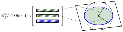
Figure 1: Illustration of $\mathbb{R}_{\leq r}^{m\times n}\cap\mathrm{Ob}(m,n)$ with $(m,n,r)=(3,4,2)$. Given a matrix $X\in\mathrm{Ob}(3,4)$, if the first two rows in the unit sphere span a plane, then the rank constraint $\operatorname{rank}(X)\leq 2$ confines the third row in the intersection of this plane with the sphere.

Graph similarity measuring.

In chemical structure comparison, biological data analysis, and web searching, measuring the similarity of two graphs is a fundamental task. Given $X\in\mathbb{R}^{m\times n}$ of which an entry evaluates the connection between two nodes in different graphs, Blondel et al. blondel2004measuresimilarity (Blo+04) proposed an iterative process to measure the desired node-to-node similarity. Furthermore, to explore the low-rank structure of the similarity matrix and to reduce the computational cost, Cason et al. cason2013iterative (CAVD13) proposed the measuring problem as follows,

$$\min_{X\in\mathbb{R}^{m\times n}} -\mathrm{tr}(X^{\top}\mathcal{L}\circ\mathcal{L}(X))$$ (1.2)

$$\mathrm{s.\,t.} \operatorname{rank}(X)\leq r,$$

$$\|X\|^{2}_{\mathrm{F}}-1=0,$$

where $\mathcal{L}:\mathbb{R}^{m\times n}\to\mathbb{R}^{m\times n}$ is a linear operator and $\|\cdot\|_{\mathrm{F}}$ denotes the Frobenius norm. Problem (1.2) falls into the scope of (P) with $h(X)=\|X\|^{2}_{\mathrm{F}}-1$ and the associated $\mathcal{H}=\mathrm{S}_{\mathrm{F}}(m,n):=\{X\in\mathbb{R}^{m\times n}:\,\|X\|^{2}_{\mathrm{F}}=1\}$.

Low-rank semidefinite programming (SDP).

Applications across various fields can be addressed by the semidefinite program,

$$\min\ \left\langle{C,Y}\right\rangle,\quad\ \mathrm{s.\,t.}\ Y\in\mathrm{Sym}(n),\,Y\succeq 0,\,\mathcal{L}(Y)=b,$$ (1.3)

where $\mathrm{Sym}(n)$ is the set of $n\times n$ symmetric matrices, $\mathcal{L}:\mathbb{R}^{n\times n}\to\mathbb{R}^{q}$ is a linear operator, and $b\in\mathbb{R}^{q}$. As shown in pataki1998lowranksolution (Pat98), a low-rank solution for (1.3) exists when the feasible region is compact. Therefore, we can employ the Burer–Monteiro factorization $Y=XX^{\top}$ burer2003BM (BM03) and impose a rank constraint on (1.3), resulting in an instance of (P),

$$\min_{X\in\mathbb{R}^{n\times n}} \langle C,XX^{\top}\rangle$$ (1.4)

$$\mathrm{s.\,t.} \operatorname{rank}(X)\leq r,$$

$$\mathcal{L}(XX^{\top})-b=0.$$

Under the conditions given in journee2010conesdp (Jou+10, BVB16), the set $\mathcal{H}=\{X\in\mathbb{R}^{n\times n}:\mathcal{L}(XX^{\top})=b\}$ is a smooth manifold. Several specific examples were considered including the oblique manifold $\mathrm{Ob}(n,n)$ goemans1995maxcutsdp (GW95), the unit Frobenius sphere $\mathrm{S}_{\mathrm{F}}(n,n)$ journee2010conesdp (Jou+10), and the stacked Stiefel manifold $\mathrm{St}(n,p)^{k}:=\{[X_{1}~X_{2}\cdots X_{k}]^{\top}\in\mathbb{R}^{kp\times n}:X_{j}\in\mathrm{St}(n,p)\text{ for }j=1,\ldots,k\}$ boumal2015blockdiagonal (Bou15), where the Stiefel manifold is defined by $\mathrm{St}(n,p):=\{X\in\mathbb{R}^{n\times p}:X^{\top}X=I_{p}\}$, and $I_{p}$ is the identity matrix of size $p\times p$.

Model reduction of Markov processes.

Numerous systems rely on Markov processes as the basic model, where each event’s probability depends only on the previous state. However, a large state space $\mathcal{S}=\{s_{1},s_{2},\ldots,s_{n}\}$, usually appearing in complicated systems, confines the identification of the Markov model $\mathrm{P}\in\mathbb{R}^{\left|{\mathcal{S}}\right|\times\left|{\mathcal{S}}\right|}$ in which an entry $\mathrm{P}(s,s^{\prime})$ represents the probability of the transition from state $s$ to state $s^{\prime}$. Therefore, we can resort to the low-rank property of the Markov process to reduce system complexity and enable tractable computations. Additionally, since the probability matrix consists of nonnegative real numbers, with each row summing to one, it is reasonable to represent $\mathrm{P}$ using the Hadamard parameterization li2023simplexHadamard (LMY23), $X\odot X,\,X\in\mathrm{Ob}(\left|{\mathcal{S}}\right|,\left|{\mathcal{S}}\right|)$. Consequently, imposing a rank constraint on $X$, we propose the following model to find reduced-dimension representations of Markov processes,

$$\min_{X\in\mathbb{R}^{\left|{\mathcal{S}}\right|\times\left|{\mathcal{S}}\right|}} \frac{1}{2}\|X\odot X-\hat{\mathrm{P}}\|^{2}_{\mathrm{F}}$$ (1.5)

$$\mathrm{s.\,t.} \operatorname{rank}(X)\leq r,$$

$$\operatorname{diag}(XX^{\top})-{\bf 1}=0,$$

where $\hat{\mathrm{P}}$ is an empirical estimate of the ground-truth $\mathrm{P}$. Formulation (1.5) provides fresh insights on identifying low-rankness in Markov processes, which will aid in extracting state features and thus facilitate various downstream tasks including state abstraction and reinforcement learning abel2018stateabstrac (Abe+18).

Reinforcement learning (RL).

To make sequential decisions in Markov processes, RL is an effective framework, which aims for the optimal policy maximizing the expected cumulative reward. Specifically, with $\mathcal{A}$ representing the action space, a policy $\pi\in\mathbb{R}^{\left|{\mathcal{S}}\right|\times\left|{\mathcal{A}}\right|}$ serves as an action selection rule, i.e., $\pi(s,a)$ gives the probability of performing action $a$ at state $s$. Moreover, in a Markov decision process (MDP), a state-action pair $(s,a)\in\mathcal{S}\times\mathcal{A}$ incurs a reward $r(s,a)$ and transitions to state $s^{\prime}\in\mathcal{S}$ with probability $\mathrm{P}_{\mathrm{d}}(s,a,s^{\prime})$, where the tensor $\mathrm{P}_{\mathrm{d}}\in\mathbb{R}^{\left|{\mathcal{S}}\right|\times\left|{\mathcal{A}}\right|\times\left|{\mathcal{S}}\right|}$ denotes the transition dynamics. Consequently, given $\mu$ as the initial state distribution and $\gamma\in(0,1)$ as the discount factor, the central task of RL is to maximize the objective $J(\pi):=\mathbb{E}[\sum_{t=0}^{\infty}\gamma^{t}r(s_{t},a_{t})\ |\ s_{0}\sim\mu,\pi]$. However, the optimization problem suffers from the curse of dimensionality when the state space $\mathcal{S}$ and the action space $\mathcal{A}$ are large sutton2018RL (SB18). To alleviate this, exploiting the low-rank structure in RL is an advisable approach. Specifically, recognizing that a policy is inherently a probability matrix, we adopt the Hadamard parameterization $\pi(X):=X\odot X,\,X\in\mathrm{Ob}(\left|{\mathcal{S}}\right|,\left|{\mathcal{A}}\right|)$, introduce a low-rank requirement on the variable $X$, and thus propose the following low-rank formulation for reinforcement learning,

$$\min_{X\in\mathbb{R}^{\left|{\mathcal{S}}\right|\times\left|{\mathcal{A}}\right|}} -J(\pi(X))$$ (1.6)

$$\mathrm{s.\,t.} \operatorname{rank}(X)\leq r,$$

$$\operatorname{diag}(XX^{\top})-{\bf 1}=0.$$

Neural network training.

Recent success in deep learning has witnessed the critical role of neural network architectures in both training efficiency and inference performance. Among various designs, two principles receive increasing attention. Typically, one is weight normalization, which expresses the weight matrix $W\in\mathbb{R}^{m\times n}$ by $W=(g{\bm{1}}^{\top})\odot X$ with $g\in\mathbb{R}^{m}$ and $X\in\mathrm{Ob}(m,n)$. Therefore, each row of $X$ encodes the direction, while $g$ is responsible for the scaling. It is reported that such a separation enhances training stability salimans2016WN (SK16). Meanwhile, another principle, namely low-rank compression, harnesses the inherent low-rankness of large-scale network weights, effectively circumventing parameter redundancy and preserving decent generalization idelbayev2020lowrankcompress (ICP20). Integrating the two principles—weight normalization and low-rank compression—presents an enlightening avenue for further development. Specifically, for the $i$-th layer in a neural network, we train the normalized weight $X_{i}$ subject to the low-rank constraint, together with scale parameters $g_{i}$, leading to the following training model,

$$\min_{\{X_{i},g_{i}\}_{i=1}^{l}} f(\{X_{i},g_{i}\}_{i=1}^{l})$$ (1.7)

$$\mathrm{s.\,t.} \operatorname{rank}(X_{i})\leq r_{i},$$

$$\operatorname{diag}(X_{i}X_{i}^{\top})-{\bf 1}=0,\ \text{for}\ i=1,2,\ldots,l,$$

where $f$ is the loss function and $l$ is the number of layers.

1.2 Motivation and related work

Apart from the aforementioned real-world applications, many problems exhibit the structure of low-rankness and orthogonal invariance. However, a unified framework to address problem (P) is lacking, which essentially suffers from three pains.

1. The optimality conditions of problem (P) remain unexplored, largely due to the involved geometry of the coupled constraints. This unawareness poses an impediment to defining stationarity measures, thereby hindering the development of algorithms.

2. The feasible region inherits the nonsmoothness of $\mathbb{R}_{\leq r}^{m\times n}$, which gives rise to the undesirable phenomenon: there exist feasible sequences along which the stationarity measures tend to zero, but with limit points non-stationary levin2023remedy (LKB23).

3. Projections onto the coupled feasible set $\mathbb{R}_{\leq r}^{m\times n}\cap\mathcal{H}$ are unclear for general $\mathcal{H}$, making it intractable to translate existing techniques in low-rank optimization, such as the projected gradient descent framework adopted by schneider2015Lojaconvergence (SU15, OGA22, OW24).

Optimality conditions.

Research on optimality conditions gains momentum in low-rank optimization, where the variational geometry, including tangent and normal cones to the feasible set, plays a pivotal role. Typically, several kinds of cones—the Mordukhovich normal cone luke2013Mordukhovich (Luk13), the Bouligand tangent cone cason2013iterative (CAVD13, SU15), and the Clarke tangent cone and the corresponding normal cone hosseini2019MordukhovichClarke (HLU19, LSX19)—to the bounded-rank set $\mathbb{R}_{\leq r}^{m\times n}$ have been well studied.

However, an additional constraint set $\mathcal{C}$ coupled with $\mathbb{R}_{\leq r}^{m\times n}$ renders the geometry of the feasible region more complicated. Specifically, when $m=n$ and $\mathcal{C}=\mathrm{Sym}(n)$, Tam et al. tam2017sparsesdp (Tam17) derived the Mordukhovich normal cone to $\mathbb{R}^{n\times n}_{\leq r}\cap\mathcal{C}$; and the Fréchet normal cones were formulated in li2020jotaspectral (LXZ20) when $\mathcal{C}$ is the intersection of $\mathrm{Sym}(n)$ with the closed unit Frobenius ball, the symmetric box or the spectrahedron. In essence, the above results stem from the symmetry of $\mathcal{C}$, which coincide with the preimages of some permutation-invariant sets $\mathcal{C}_{\mathrm{p}}\subseteq\mathbb{R}^{n}$ under the eigenvalue map. This observation reduces the low-rankness of matrices in $\mathcal{C}$ to the sparsity of vectors in $\mathcal{C}_{\mathrm{p}}$. Therefore, computing the normal cone to $\{v\in\mathbb{R}^{n}:\|v\|_{0}\leq r\}\cap\mathcal{C}_{\mathrm{p}}$ by (pan2017restrictedLICQ, PLX17, Proposition 3.2) and applying (lewis1996groupinvariance, Lew96, Theorem 8.3) recover the results in tam2017sparsesdp (Tam17, LXZ20), where $\|\cdot\|_{0}$ denotes the cardinality of a vector. It is worth noting that these developments require the matrix variable to be square and symmetric; but when $m\neq n$ breaks the symmetry, existing results on sparsity optimization pan2017restrictedLICQ (PLX17) no longer apply, which necessitates analysis tailored for the geometry of the coupled feasible region.

Recently, Li and Luo li2023normalboundedaffine (LL23) characterized the normal cone to $\mathbb{R}_{\leq r}^{m\times n}\cap\mathcal{C}$ with $\mathcal{C}$ as an affine manifold. More relevantly, a closed-form expression of the tangent cone to $\mathbb{R}_{\leq r}^{m\times n}\cap\mathrm{S}_{\mathrm{F}}(m,n)$ was given in cason2013iterative (CAVD13), which turns out to be a special instance of the feasible region in problem (P).

Optimization on bounded-rank matrices.

In general, finding a global minimizer of a function solely subject to the bounded-rank constraint is NP-hard gillis2011NPlowrank (GG11). Existing literature schneider2015Lojaconvergence (SU15, LKB23, OA23) reveals that it remains possible to compute a (first-order) B-stationary point, a zero of the B-stationarity measure—norm of the projection of negative gradient onto the Bouligand tangent cone to $\mathbb{R}_{\leq r}^{m\times n}$. However, the nonsmooth and nonconvex nature of the bounded-rank set introduces the main obstacles. Typically, the apocalypse exists, which characterizes the sequence of points with B-stationarity measures converging to zero, but limit points not B-stationary levin2023remedy (LKB23). A line of algorithms is developed for the optimization on bounded-rank matrices, and they are categorized into three groups.

The first group is based on the projected gradient descent (PGD) framework, i.e., updating the iterate along an appropriate direction and then projecting it onto the bounded-rank set, which amounts to computing a truncated singular value decomposition (SVD) of a matrix. The PGD method in olikier2024PGD (OW24) has recently been proven to accumulate at B-stationary points. However, the well-known $\mathrm{P^{2}GD}$ schneider2015Lojaconvergence (SU15), additionally projecting negative gradient onto the tangent cone as the search direction, can result in the apocalypse; an explicit example was given in levin2023remedy (LKB23). To resolve this, Olikier et al. olikier2022P2GDR (OGA22) introduced a rank-adaptive strategy and obtained a modification $\mathrm{P^{2}GDR}$.

The second group evolves around the retraction-free principle. In detail, search directions are chosen from the so-called restricted tangent cone to $\mathbb{R}_{\leq r}^{m\times n}$ (see olikier2023RFDR (OA23)) such that updates are performed along straight lines, and thus the algorithm gets rid of expensive projections onto the bounded-rank set. The original retraction-free descent (RFD) method schneider2015Lojaconvergence (SU15) may encounter the apocalypse, and the variant RFDR olikier2023RFDR (OA23) equipped with a rank reduction mechanism is guaranteed with the convergence to B-stationary points. Recently, Olikier and Absil olikier2024ERFDR (OA24) proposed a more efficient version named ERFDR, which preserves the benign convergence property of RFDR.

The third group resorts to the parameterization of the bounded-rank set, which constructs a smooth manifold $\mathcal{M}$ and an associated mapping $\phi$ such that $\phi(\mathcal{M})=\mathbb{R}_{\leq r}^{m\times n}$. Subsequently, the original problem on the bounded-rank set can be reformulated as minimizing $\bar{f}:=f\circ\phi$ over $\mathcal{M}$, a Riemannian optimization problem. For instance, the LR lift park2018findingLR (Par+18, HLB20) uses $\phi(L,R)=LR^{\top}$ to factorize the low-rank matrix. Levin et al. levin2024effectlift (LKB24) proposed the parameterization $\phi(U,S,V)=USV^{\top}$ with symmetric $S$ and orthogonal $U$ and $V$. Moreover, viewing the bounded-rank set as the determinantal variety harris1992algebraic (Har92), Khrulkov and Ivanoseledts khrulkov2018desingularization (KO18) derived the desingularization, which is a modified version of the classical Room–Kempf procedure room1938 (Roo38, Kem73), and its geometry was further explored in a recent work rebjock2024boundedrank (RB24). A benefit of these parameterizations is the ability to circumvent the apocalypse; see levin2024effectlift (LKB24).

Translating the existing methods to address problem (P) appears challenging. In general, the PGD-based method stagnates due to the unknown projection onto the coupled feasible set. The retraction-free technique relies on the specific structure of $\mathbb{R}_{\leq r}^{m\times n}$ while the additional constraint $\mathcal{H}$ distorts the landscape, presenting obstacles to promoting the technique. Moreover, finding a parameterization for $\mathbb{R}_{\leq r}^{m\times n}\cap\mathcal{H}$ requires new insights, and in this scenario, the equivalence between the reformulated problem and the original problem is worth further investigation.

1.3 Contributions

In this paper, we develop a space-decoupling framework by taking advantage of the geometry of the bounded-rank set and the extra orthogonally invariant constraints. The space-decoupling principle features the following aspects.

General properties of the orthogonally invariant mapping $h$ are studied, which turn out to be closely related to rank information of the matrix variable. Specifically, Assumption 1 reveals that $\mathcal{H}$—the level set of $h$—is a smooth manifold, and we show that $h$ also induces a series of manifolds $\mathcal{H}^{s}$ embedded in lower-dimensional spaces $\mathbb{R}^{m\times s}$ ($s=1,2,\ldots,n$). Notably, these $\mathcal{H}^{s}$ inherit the geometric structure from $\mathcal{H}$, and the tangent space to $\mathcal{H}$ at $X$ can be decoupled into a tangent space to $\mathcal{H}^{s}$ and the space orthogonal to $X$ (Proposition 3). The results build up a connection between $\mathbb{R}_{\leq r}^{m\times n}$ and $\mathcal{H}$, paving the way for investigating $\mathbb{R}_{\leq r}^{m\times n}\cap\mathcal{H}$.

We give a closed-form expression for the tangent cone to the coupled feasible set (Theorem 3.1), which essentially unveils the intersection rule—the tangent (resp. normal) cone to $\mathbb{R}_{\leq r}^{m\times n}\cap\mathcal{H}$ can be decomposed as the intersection (resp. direct sum) of tangent (resp. normal) cones to each of them, i.e.,

$$\mathrm{T}_{X}\left({\mathbb{R}_{\leq r}^{m\times n}\cap\mathcal{H}}\right) =\mathrm{T}_{X}\mathbb{R}_{\leq r}^{m\times n}\cap\mathrm{T}_{X}\mathcal{H},$$

$$\mathrm{N}_{X}\left({\mathbb{R}_{\leq r}^{m\times n}\cap\mathcal{H}}\right) =\mathrm{N}_{X}\mathbb{R}_{\leq r}^{m\times n}\oplus\mathrm{N}_{X}\mathcal{H}.$$

Moreover, the optimality conditions for (P) are developed.

Viewing the Grassmann manifold as embedded in $\mathrm{Sym}(n)$, i.e., $\mathrm{Gr}(n,s):=\{G\in\mathrm{Sym}(n):G^{2}=G,\,\operatorname{rank}(G)=s\}$, we propose the following space-decoupling parameterization,

$$\mathcal{M}_{h}:=\left\{(X,G)\in\mathbb{R}^{m\times n}\times\mathrm{Gr}(n,n-r):XG=0,\ h(X)=0\right\}$$

with the smooth mapping $\phi:\mathbb{R}^{m\times n}\times\mathrm{Sym}(n)\to\mathbb{R}^{m\times n}:(X,G)\mapsto X$ satisfying $\phi(\mathcal{M}_{h})=\mathbb{R}_{\leq r}^{m\times n}\cap\mathcal{H}$. We prove that the set $\mathcal{M}_{h}$ is a smooth manifold (Theorem 4.1), and thus reformulate the original nonsmooth coupled-constrained optimization problem as a smooth Riemannian optimization problem,

$$\min_{(X,G)\in\mathcal{M}_{h}}\bar{f}(X,G):=f\circ\phi(X,G). {\mathcal{M}_{h}}$$ (P-)

Specifically, an element $(X,G)$ in $\mathcal{M}_{h}$ has two coordinates, with $X$ subject to the orthogonally invariant constraints and $G$ encodes the rank information. In this manner, the parameterization decouples the intertwined constraints into two spaces; see Fig. 2 for an illustrative diagram.

Figure 2: Illustration of optimization via the space-decoupling parameterization.

To facilitate Riemannian optimization methods, we provide Riemannian derivatives, retractions, and vector transports on $\mathcal{M}_{h}$. It reveals that implementing Riemannian algorithms on $\mathcal{M}_{h}$ is painless if the geometry of $\mathcal{H}$ is understood a prior. Moreover, we identify the equivalence between the reformulated and the original optimization problems (Theorem 5.1): if $(X,G)$ is a second-order stationary point for (P-${\mathcal{M}_{h}}$) then $X=\phi(X,G)$ is a first-order stationary point for (P); and when $\operatorname{rank}(X)=r$, the first-stationarity of $(X,G)$ for (P-${\mathcal{M}_{h}}$) concludes the first-stationarity of $X$ for (P). Convergence guarantees for the algorithms on $\mathcal{M}_{h}$ are also provided.

The effectiveness and efficiency of the proposed framework are validated by fruitful numerical experiments across applications discussed in section 1.1. Note that the proposed models—(1.5) for Markov process reduction, (1.6) for low-rank reinforcement learning, and (1.7) for deep learning—exhibit good performance and thus contribute to their respective fields. In practice, Riemannian algorithms generate a sequence $\{(X_{k},G_{k})\}$ on $\mathcal{M}_{h}$, ensuring that $\{X_{k}\}$ satisfies the constraints of (P). This fact is favorable not only to the early stopping of an algorithm when a feasible solution is required but also to some specific problems (e.g., (1.6)) where the objective cannot be defined outside of the feasible region.

1.4 Notation

Let $\mathbb{R}^{m\times n}_{s}=\{X\in\mathbb{R}^{m\times n}:\operatorname{rank}(X)=s\}$ be the set of fixed-rank matrices, and $\mathrm{Skew}(n):=\{\Omega\in\mathbb{R}^{n\times n}:\,\Omega^{\top}=-\Omega\}$ be the set of skew-symmetric matrices. The symmetric part of a square matrix is defined by $\mathrm{sym}(M):=\frac{1}{2}(M+M^{\top})$. Given a smooth manifold $\mathcal{X}$, $\mathrm{T}\mathcal{X}$ denotes the tangent bundle, and $\mathrm{T}_{X}\mathcal{X}$ denotes the tangent space at $X\in\mathcal{X}$. Given a mapping $F:\mathcal{X}_{1}\to\mathcal{X}_{2}$ between two manifolds, $\mathrm{D}F_{X}:\mathrm{T}_{X}\mathcal{X}_{1}\to\mathrm{T}_{F(X)}\mathcal{X}_{2}$ denotes the differential of $F$ at $X\in\mathcal{X}_{1}$. Given a matrix $V\in\mathrm{St}(n,r)$, $V_{\bot}$ is an orthonormal completion of it in the sense of $[V\ V_{\bot}]\in\mathcal{O}(n)$. The standard inner product in an Euclidean space is given by $\left\langle{X_{1},X_{2}}\right\rangle:=\mathrm{tr}(X_{1}^{\top}X_{2})$. Let $\mathcal{P}_{\mathcal{X}}$ denote the projection onto the set $\mathcal{X}$.

1.5 Organization

In section 2, we investigate the general properties of the orthogonally invariant mapping $h$ and the associated level set $\mathcal{H}$. The tangent and normal cones to the coupled feasible region are identified, and the optimality conditions are also formulated in section 3. Section 4 proposes the space-decoupling parameterization $\mathcal{M}_{h}$ and its Riemannian geometry. In section 5, we specify the Riemannian derivatives, retractions, and vector transports on $\mathcal{M}_{h}$, analyze the equivalence between (P-${\mathcal{M}_{h}}$) and (P), and provide the convergence guarantees for Riemannian algorithms. Section 6 reports the numerical performance of the proposed framework. Finally, we draw the conclusion in section 7.

2 Properties of the orthogonally invariant mapping

This section uncovers the connection between the orthogonal invariance of the mapping $h$ and the rank information of the variable $X$, and thus bridges the geometry of $\mathcal{H}$ and $\mathbb{R}_{\leq r}^{m\times n}$.

The Bouligand tangent cone to a set $\mathcal{X}$ at a point $X\in\mathcal{X}$ is

$$\mathrm{T}_{X}\mathcal{X}:=\left\{\eta=\lim_{k\rightarrow\infty}\frac{\left(X_{k}-X\right)}{t_{k}}:\ X_{k}\in\mathcal{X},t_{k}>0\ \text{for all}\,\,k,\lim_{k\rightarrow\infty}t_{k}=0\right\}.$$

A vector $\eta\in\mathrm{T}_{X}\mathcal{X}$ is derivable if it admits a curve $\gamma(t)$ on $\mathcal{X}$ with $\gamma(0)=X$ and $\gamma^{\prime}(0)=\eta$, and the set $\mathcal{X}$ is geometrically derivable at $X$ if any vector in $\mathrm{T}_{X}\mathcal{X}$ is derivable. Taking the polar operation on $\mathrm{T}_{X}\mathcal{X}$ introduces the Fréchet normal cone, $\mathrm{N}_{X}\mathcal{X}:=\left({\mathrm{T}_{X}\mathcal{X}}\right)^{\circ}$. Specifically, if $\mathcal{X}$ is a smooth manifold, the tangent (resp. normal) cone reduces to a vector space, i.e., the tangent (resp. normal) space.

2.1 Geometry of $\mathcal{H}$

The full-rankness of $h$ in Assumption 1 implies that the level set $\mathcal{H}$ is a smooth manifold embedded in $\mathbb{R}^{m\times n}$; see (lee2012manifolds, Lee12, Corollary 5.14). Moreover, the orthogonal invariance of $h$ sheds light on the fact that the tangent space $\mathrm{T}_{X}\mathcal{H}$ contains a subspace that is independent of the choice of $h$; see the following proposition.

Proposition 1

Given $X\in\mathcal{H}$ with $\operatorname{rank}{(X)}=s$ and the SVD $X=U\varSigma V^{\top}$, it holds that

$$\mathcal{K}_{X}:=\left\{{U\varSigma\Omega V^{\top}+BV_{\bot}^{\top}:\,\Omega\in\mathrm{Skew}(s),\,B\in\mathbb{R}^{m\times(n-s)}}\right\}\subseteq\mathrm{T}_{X}\mathcal{H}.$$ (2.1)

Proof

The fact $\mathrm{T}_{X}\mathcal{H}=\operatorname{ker}(\mathrm{D}h_{X})$ shifts the focus to prove $\mathcal{K}_{X}\subseteq\operatorname{ker}(\mathrm{D}h_{X})$. Notice that $\mathcal{K}_{X}$ is a linear space and any $\eta\in\mathcal{K}_{X}$ can be expressed in the form of $\eta=\eta_{1}+\eta_{2}$ where $\eta_{1}=U\varSigma\Omega V^{\top}+UB_{1}V_{\bot}^{\top}$ and $\eta_{2}=U_{\bot}B_{2}V_{\bot}^{\top}$ with $\Omega\in\mathrm{Skew}\left({s}\right),\,B_{1}\in\mathbb{R}^{s\times\left({n-s}\right)}$, and $B_{2}\in\mathbb{R}^{\left({m-s}\right)\times\left({n-s}\right)}$.

We first validate $\eta_{1}\in\operatorname{ker}(\mathrm{D}h_{X})$. In view of the orthogonal invariance of $h$, the mapping $F:\mathrm{St}(n,s)\rightarrow\mathbb{R}^{q}:\,\tilde{V}\mapsto h(U\varSigma\tilde{V}^{\top})$ is constant since $F(\tilde{V})=h(U\varSigma\tilde{V}^{\top})=h(XQ_{V}Q_{\tilde{V}}^{\top})=h(X)$ where $Q_{V}:=[{V}\,\,{V}_{\bot}]\in\mathcal{O}(n)$ and $Q_{\tilde{V}}:=[\tilde{V}\,\,\tilde{V}_{\bot}]\in\mathcal{O}(n)$. Therefore, the differential $\mathrm{D}F_{\tilde{V}}\equiv 0$ for all $\tilde{V}\in\mathrm{St}(n,s)$ including $V$. Taking into account the tangent space $\mathrm{T}_{{V}}\mathrm{St}(n,s)$ (see (absil2008optimization, Abs08, §3.5)) and given ${\xi}=-V\Omega+V_{\bot}B_{1}^{\top}\varSigma^{-1}\in\mathrm{T}_{{V}}\mathrm{St}(n,s)$, it holds that $\mathrm{D}{h}_{X}[\eta_{1}]=\mathrm{D}{h}_{X}[U\varSigma{\xi}^{\top}]=\frac{\mathrm{d}}{\mathrm{d}t}h(X+tU\varSigma{\xi}^{\top})\big{|}_{t=0}=\frac{\mathrm{d}}{\mathrm{d}t}F(V+t{\xi})\big{|}_{t=0}=\mathrm{D}F_{{V}}[{\xi}]=0$.

Due to the orthogonal invariance of $h$, it is direct to obtain $h(X+t\eta_{2})=h((X+t\eta_{2})Q)=h(X-t\eta_{2})$ for $t\in\mathbb{R}$ with $Q=[{V}\,-\!{V}_{\bot}]\in\mathcal{O}(n)$. Thus, it implies $\mathrm{D}h_{X}[\eta_{2}]=\frac{\mathrm{d}}{\mathrm{d}t}h\left(X+t\eta_{2}\right)\big{|}_{t=0}=0$.

The following corollary reveals that any element orthogonal to $X$ falls into $\mathrm{T}_{X}\mathcal{H}$, which plays an important role in subsequent developments.

Corollary 1

Given $X\in\mathcal{H}$, if $Y\in\mathbb{R}^{m\times n}$ satisfies $XY^{\top}=0$, it holds that $Y\in\mathrm{T}_{X}\mathcal{H}=\operatorname{ker}(\mathrm{D}h_{X})$.

Proof

The SVD of $X=U\varSigma V$ and $XY^{\top}=0$ imply that $Y=BV_{\bot}^{\top}$, which is in the subspace $\mathcal{K}_{X}\subseteq\mathrm{T}_{X}\mathcal{H}$ from Proposition 1.

Proposition 1 demonstrates that for any orthogonally invariant $h$, there is a subset $\mathcal{K}_{X}\subseteq\mathrm{T}_{X}\mathcal{H}$. Taking the polar operation on both sides yields $\mathrm{N}_{X}\mathcal{H}=\left({\mathrm{T}_{X}\mathcal{H}}\right)^{\circ}\subseteq\mathcal{K}_{X}^{\circ}$, which leads to the following lemma.

Lemma 1

Given $X\in\mathcal{H}$ with $\operatorname{rank}{(X)}=s$ and the SVD $X=U\varSigma V^{\top}$, it holds that

$$\mathrm{N}_{X}\mathcal{H}\subseteq\mathcal{K}_{X}^{\circ}=\left\{AX:\ A\in\mathbb{R}^{m\times m},\ U^{\top}AU\in\mathrm{Sym}(s)\right\}.$$ (2.2)

Proof

It suffices to identify $\mathcal{K}_{X}^{\circ}$, which is the orthonormal completion of the linear space $\mathcal{K}_{X}$. Specifically, any $\eta\in\mathbb{R}^{m\times n}$ can be expressed in the form of $\eta=AX+\tilde{A}V_{\bot}^{\top}$ with $A\in\mathbb{R}^{m\times m}$ and $\tilde{A}\in\mathbb{R}^{m\times\left(n-s\right)}$. It follows from $\eta\in\mathcal{K}_{X}^{\circ}$ and the expression of $\mathcal{K}_{X}$ in (2.1) that $\langle AX+\tilde{A}V_{\bot}^{\top},U\varSigma\Omega V^{\top}+BV_{\bot}^{\top}\rangle=0$ for all $\Omega\in\mathrm{Skew}(s)$ and $B\in\mathbb{R}^{m\times(n-s)}$, reducing to ${\langle AU\varSigma,U\varSigma\Omega\rangle+\langle\tilde{A},B\rangle=0}$. Consequently, the arbitrariness of $\Omega$ and $B$ implies $U^{\top}AU\in\mathrm{Sym}(s)$ and $\tilde{A}=0$.

Note that the developed properties of $\mathcal{H}$ extract the rank of $X$ via the singular value decomposition, and thus link the orthogonal invariance of $h$ to the rank information.

2.2 Inheritance principle

Based on the above results, we demonstrate that the properties of $h$ can be inherited from $\mathbb{R}^{m\times n}$ to lower-dimensional spaces. For $s=1,2,\ldots,n$, we define a sequence of natural embeddings $i^{s}:\,\mathbb{R}^{m\times s}\rightarrow\mathbb{R}^{m\times n}:\,H\mapsto[H\ 0^{m\times\left({n-s}\right)}]$, the associated mappings $h^{s}:=h\circ i^{s}$, and the level sets

$$\mathcal{H}^{s}:=\left\{{H\in\mathbb{R}^{m\times s}:h^{s}(H)=0}\right\}.$$

Given $X\in\mathbb{R}^{m\times n}$. The developments of this subsection rely on a decomposition $X=HV^{\top}$ with $H\in\mathbb{R}^{m\times s}$ and $V\in\mathrm{St}(n,s)$, which is always achievable in practice; e.g., singular value decomposition and QR factorization. Subsequently, $h$ and $h^{s}$ are connected via the values and differentials.

Lemma 2

Given $X\in\mathbb{R}^{m\times n}$ with a decomposition $X=HV^{\top}$ where $H\in\mathbb{R}^{m\times s}$ and $V\in\mathrm{St}(n,s)$, it follows that

$$h(X)=h^{s}(H)\quad\text{and}\quad\mathrm{D}h_{X}[KV^{\top}]=\mathrm{D}h^{s}_{H}[K]\quad\text{for all}\ K\in\mathbb{R}^{m\times s}.$$

Moreover, $X\in\mathcal{H}$ if and only if $H\in\mathcal{H}^{s}$.

Proof

Let $Q=[V\,\,V_{\bot}]\in\mathcal{O}(n)$. It follows from the orthogonal invariance of $h$ and $XQ=[H\,\,0^{m\times(n-s)}]$ that $h(X)=h(XQ)=h^{s}(H)$. Moreover, $h^{s}=h\circ i^{s}$ implies that $\mathrm{D}h^{s}_{H}[K]=\mathrm{D}h_{i^{s}(H)}[i^{s}(K)]=\mathrm{D}h_{XQ}[KV^{\top}Q]=\frac{\mathrm{d}}{\mathrm{d}t}h(XQ+tKV^{\top}Q)\big{|}_{t=0}=\frac{\mathrm{d}}{\mathrm{d}t}h(X+tKV^{\top})\big{|}_{t=0}=\mathrm{D}h_{X}[KV^{\top}]$.

Lemma 2 indicates that $h^{s}$ is also orthogonally invariant, which inspires us to generalize the property from $\mathcal{H}$ to $\mathcal{H}^{s}$. The following proposition shows $\mathcal{H}^{s}$ is a smooth manifold embedded in a lower-dimensional space.

Proposition 2

If $\mathcal{H}^{s}$ is nonempty, then it is an embedded submanifold in $\mathbb{R}^{m\times s}$ of dimension $(ms-q)$.

Proof

We aim to show $\mathrm{D}h^{s}$ is full-rank in the level set $\mathcal{H}^{s}$. Using Corollary 1, we find $\{\left[{0^{m\times{s}}\,\,C}\right]:C\in\mathbb{R}^{m\times\left({n-s}\right)}\}\subseteq\operatorname{ker}(\mathrm{D}h_{i^{s}(H)})$ for $H\in\mathcal{H}^{s}$. This observation, together with the full-rankness of $\mathrm{D}h$, reveals that any $b\in\mathbb{R}^{q}$ admits a preimage $\eta$ in the form of $\eta=[\eta^{s}\,\,0^{m\times(n-s)}]\in\mathbb{R}^{m\times n}$, and thus $b=\mathrm{D}h_{i^{s}({H})}[\eta]=\mathrm{D}h^{s}_{H}[\eta^{s}]$. The arbitrariness of $H\in\mathcal{H}^{s}$ and $b\in\mathbb{R}^{q}$ implies $\mathrm{D}h^{s}$ has the full rank $q$ in $\mathcal{H}^{s}$. At last, we apply (lee2012manifolds, Lee12, Corollary 5.14) to arrive at the conclusion.

In succession, we show the relationship between the geometry of $\mathcal{H}$ and $\mathcal{H}^{s}$.

Proposition 3

Given $X\in\mathbb{R}^{m\times n}$ with a decomposition $X=HV^{\top}$ where $H\in\mathbb{R}^{m\times s}$ and $V\in\mathrm{St}(n,s)$, it holds that

$$\mathrm{T}_{X}\mathcal{H}= \left\{{KV^{\top}+BV^{\top}_{\bot}:\ K\in\mathrm{T}_{H}\mathcal{H}^{s},\,B\in\mathbb{R}^{m\times(n-s)}}\right\}$$ (2.3)

$$= \left({\mathrm{T}_{H}\mathcal{H}^{s}}\right)V^{\top}\oplus\left({\mathbb{R}^{m\times(n-s)}}\right)V^{\top}_{\bot},$$ (2.4)

where $\oplus$ denotes the direct sum. Moreover,

$$\mathrm{N}_{X}\mathcal{H}=\left\{{NV^{\top}:\ N\in\mathrm{N}_{H}\mathcal{H}^{s}}\right\}=\left({\mathrm{N}_{H}\mathcal{H}^{s}}\right)V^{\top}.$$ (2.5)

Proof

By Lemma 2, we have $\mathrm{D}h_{X}[KV^{\top}]=\mathrm{D}h^{s}_{H}[K]=0$ for $K\in\mathrm{T}_{H}\mathcal{H}^{s}$, which implies $KV^{\top}\in\mathrm{T}_{X}\mathcal{H}$, and thus $\left({\mathrm{T}_{H}\mathcal{H}^{s}}\right)V^{\top}\subseteq\mathrm{T}_{X}\mathcal{H}$. Combining this result with $\{BV^{\top}_{\bot}:\ B\in\mathbb{R}^{m\times(n-s)}\}\subseteq\mathrm{T}_{X}\mathcal{H}$ revealed by (2.1), we conclude the “$\supseteq$” part of the equality in (2.3). Moreover, the dimension of the space on the right side of (2.3) is $\operatorname{dim}(\mathcal{H}^{s})+\operatorname{dim}(\mathbb{R}^{m\times(n-s)})=(ms-q)+m(n-s)=mn-q$, which coincides with $\operatorname{dim}(\mathrm{T}_{X}\mathcal{H})$. Therefore, we confirm the equality in (2.3). Taking the orthogonal complement on both sides leads to $\mathrm{N}_{X}\mathcal{H}=\left({\mathrm{N}_{H}\mathcal{H}^{s}}\right)V^{\top}$.

Proposition 3 decomposes $\mathrm{T}_{X}\mathcal{H}$ into two components: one originating from the tangent space to $\mathcal{H}^{s}$ and the other orthogonal to $X$. As a byproduct, it is straightforward from (2.4) that

$$\mathrm{T}_{H}\mathcal{H}^{s}=\left({\mathrm{T}_{X}\mathcal{H}}\right)V.$$

In other words, the geometry of $\mathcal{H}$ enlightens that of $\mathcal{H}^{s}$.

Consequently, computing the projection of $E\in\mathbb{R}^{m\times n}$ onto $\mathrm{T}_{X}\mathcal{H}$ reduces to the following optimization problem,

$$\operatorname*{arg\,min}_{K\in\mathrm{T}_{H}\mathcal{H}^{s},\,B\in\mathbb{R}^{m\times(n-s)}}\|E-(KV^{\top}+BV^{\top}_{\bot})\|_{\mathrm{F}}^{2}=\|EV-K\|_{\mathrm{F}}^{2}+\|{EV_{\bot}-B}\|_{\mathrm{F}}^{2}.$$

Collecting the solution $K^{*}=\mathcal{P}_{\mathrm{T}_{H}\mathcal{H}^{s}}(EV),\,B^{*}=EV_{\bot}$ yields

$$\mathcal{P}_{\mathrm{T}_{X}\mathcal{H}}(E)=\mathcal{P}_{\mathrm{T}_{H}\mathcal{H}^{s}}(EV)V^{\top}+EV_{\bot}V_{\bot}^{\top}.$$ (2.6)

3 Optimality conditions

In this section, we explore the geometry of $\mathbb{R}_{s}^{m\times n}\cap\mathcal{H}$, and then employ the results to identify the tangent and normal cones to $\mathbb{R}_{\leq r}^{m\times n}\cap\mathcal{H}$. Consequently, the optimality conditions for problem (P) are derived.

The geometry of low-rank sets is well developed; see vandereycken2013lowrankcompletion (Van13, SU15). As a fixed-rank layer of $\mathbb{R}_{\leq r}^{m\times n}$, $\mathbb{R}_{s}^{m\times n}$ is indeed an analytic manifold. Given $X\in\mathbb{R}_{s}^{m\times n}$ with the singular value decomposition $X=U\varSigma V^{\top}$, the tangent and normal spaces are outlined below,

$$\mathrm{T}_{X}\mathbb{R}_{s}^{m\times n}=\left\{{\left[U\,\,U_{\bot}\right]\left[\begin{matrix}\mathbb{R}^{s\times s}&\mathbb{R}^{s\times\left(n-s\right)}\\ \mathbb{R}^{\left(m-s\right)\times s}&0^{\left(m-s\right)\times\left(n-s\right)}\\ \end{matrix}\right]\left[V\,\,V_{\bot}\right]^{\top}}\right\},$$ (3.1)

$$\mathrm{N}_{X}\mathbb{R}_{s}^{m\times n}=\left\{{\left[U\,\,U_{\bot}\right]\left[\begin{matrix}0^{s\times s}&0^{s\times\left(n-s\right)}\\ 0^{\left(m-s\right)\times s}&\mathbb{R}^{\left(m-s\right)\times\left(n-s\right)}\\ \end{matrix}\right]\left[V\,\,V_{\bot}\right]^{\top}}\right\}.$$ (3.2)

Assembling the layers $\mathbb{R}_{s}^{m\times n}\ (s=0,1,\ldots,r)$ yields the bounded-rank set $\mathbb{R}_{\leq r}^{m\times n}$, with its tangent and normal cones at $X$ formulated as follows,

$$\mathrm{T}_{X}\mathbb{R}_{\leq r}^{m\times n}=\mathrm{T}_{X}\mathbb{R}_{s}^{m\times n}+\left\{{N\in\mathrm{N}_{X}\mathbb{R}_{s}^{m\times n}:\ \operatorname{rank}\left({N}\right)\leq r-s}\right\},$$ (3.3)

$$\mathrm{N}_{X}\mathbb{R}_{\leq r}^{m\times n}=\begin{cases}\mathrm{N}_{X}\mathbb{R}_{s}^{m\times n},\,\,\quad if\,\,s=r,\\ \left\{0\right\},\,\,\quad\quad\quad\ \,if\,\,s<r.\end{cases}$$ (3.4)

Let $P_{W}:=WW^{\top}$. The projection of $E\in\mathbb{R}^{m\times n}$ onto $\mathrm{T}_{X}\mathbb{R}_{\leq r}^{m\times n}$ is given by

$$\mathcal{P}_{\mathrm{T}_{X}\mathbb{R}_{\leq r}^{m\times n}}(E)=EP_{V}+P_{U}EP_{V_{\bot}}+\mathcal{P}_{\mathbb{R}^{m\times n}_{r-s}}\left({P_{U_{\bot}}EP_{V_{\bot}}}\right).$$ (3.5)

3.1 Variational geometry

Armed with the properties of $\mathbb{R}_{\leq r}^{m\times n}$ and those of $\mathcal{H}$ obtained in section 2, we delve into the geometry of their intersection. To this end, we first revisit the basics for tangent and normal cones to the union (or intersection) of finite sets; see rockafellar2009variationalanalysis (RW09, Lee12).

• If $X\in\bigcup_{i=1}^{d}{\mathcal{X}_{i}}$, then it holds $\mathrm{T}_{X}(\bigcup\nolimits_{i=1}^{d}{\mathcal{X}_{i}})=\bigcup\nolimits_{i=1}^{d}\mathrm{T}_{X}\mathcal{X}_{i}$;

• If $X\in\mathcal{X}_{1}\cap\mathcal{X}_{2}$, then it holds

  $$\mathrm{T}_{X}\left({\mathcal{X}_{1}\cap\mathcal{X}_{2}}\right)\subseteq\mathrm{T}_{X}\mathcal{X}_{1}\cap\mathrm{T}_{X}\mathcal{X}_{2},\quad\text{and}\quad\ \mathrm{N}_{X}\left({\mathcal{X}_{1}\cap\mathcal{X}_{2}}\right)\supseteq\mathrm{N}_{X}\mathcal{X}_{1}+\mathrm{N}_{X}\mathcal{X}_{2};$$ (3.6)

• If both $\mathcal{X}_{1}$ and $\mathcal{X}_{2}$ are smooth manifolds and intersect transversally, i.e., for any $X\in\mathcal{X}_{1}\cap\mathcal{X}_{2}$, $\mathrm{T}_{X}{\mathcal{X}_{1}}+\mathrm{T}_{X}{\mathcal{X}_{2}}=\mathbb{R}^{m\times n},\ \text{or equivalently,}\ \mathrm{N}_{X}\mathcal{X}_{1}\cap\mathrm{N}_{X}\mathcal{X}_{2}=\{0\}$, then $\mathcal{X}_{1}\cap\mathcal{X}_{2}$ is also a smooth manifold with

  $$\mathrm{T}_{X}\left({\mathcal{X}_{1}\cap\mathcal{X}_{2}}\right)=\mathrm{T}_{X}\mathcal{X}_{1}\cap\mathrm{T}_{X}\mathcal{X}_{2},\quad\text{and}\quad\ \mathrm{N}_{X}\left({\mathcal{X}_{1}\cap\mathcal{X}_{2}}\right)=\mathrm{N}_{X}\mathcal{X}_{1}+\mathrm{N}_{X}\mathcal{X}_{2}.$$ (3.7)

Generally, studying the geometry of the constraints in problem (P) is hindered by the nonsmoothness of $\mathbb{R}_{\leq r}^{m\times n}$, for which the rule (3.7) fails. To circumvent this, we take advantage of the structure $\mathbb{R}_{\leq r}^{m\times n}=\bigcup_{s=0}^{r}\mathbb{R}_{s}^{m\times n}$, and turn to characterize $\mathrm{T}_{X}\mathbb{R}_{s}^{m\times n}\cap\mathrm{T}_{X}\mathcal{H}$ as the first step.

Proposition 4

For $s=0,1,\ldots,r$, given $X\in\mathbb{R}_{s}^{m\times n}\cap\mathcal{H}$ with the singular value decomposition $X=U\varSigma V^{\top}=HV^{\top}$ where $H=U\varSigma$, it holds that

$$\mathrm{T}_{X}\mathbb{R}_{s}^{m\times n}\cap\mathrm{T}_{X}\mathcal{H}=\left\{{KV^{\top}+UJV_{\bot}^{\top}:\ K\in\mathrm{T}_{H}\mathcal{H}^{s},\,J\in\mathbb{R}^{s\times(n-s)}}\right\}.$$ (3.8)

Proof

Given a tangent vector $\eta=KV^{\top}+UJV_{\bot}^{\top}\in\mathrm{T}_{X}\mathbb{R}_{s}^{m\times n}$ from (3.1). If additionally $\eta\in\mathrm{T}_{X}\mathcal{H}$, i.e., $\mathrm{D}h_{X}[KV^{\top}+UJV_{\bot}^{\top}]=0$, we have $\mathrm{D}h_{X}[KV^{\top}]=0$ since $UJV_{\bot}^{\top}\in\operatorname{ker}(\mathrm{D}h_{X})$ via Corollary 1. Applying Lemma 2 shows $K\in\operatorname{ker}(\mathrm{D}h^{s}_{H})=\mathrm{T}_{H}\mathcal{H}^{s}$, which concludes the “$\subseteq$” part in (3.8). Moreover, the “$\supseteq$” part results from the expressions (2.3) and (3.1).

In fact, if $\mathbb{R}_{s}^{m\times n}\cap\mathcal{H}$ is nonempty, then it is a smooth manifold. To see this, recall from Lemma 1 that an element in $\mathrm{N}_{X}\mathcal{H}$ has the form of $AX$ for some $A\in\mathbb{R}^{m\times m}$. If $AX$ also belongs to $\mathrm{N}_{X}\mathbb{R}_{s}^{m\times n}$, then from (3.2) identifying $\mathrm{N}_{X}\mathbb{R}_{s}^{m\times n}$, we can derive $AX=0$, and thus ${\mathrm{N}_{X}\mathbb{R}_{s}^{m\times n}\cap\mathrm{N}_{X}\mathcal{H}=\left\{{0}\right\}}$, which implies $\mathbb{R}_{s}^{m\times n}$ and $\mathcal{H}$ intersect transversally. Therefore, ${\mathbb{R}_{s}^{m\times n}\cap\mathcal{H}}$ is a smooth manifold with

$$\mathrm{T}_{X}\left({\mathbb{R}_{s}^{m\times n}\cap\mathcal{H}}\right)=\mathrm{T}_{X}\mathbb{R}_{s}^{m\times n}\cap\mathrm{T}_{X}\mathcal{H}.$$

In view of this fact, Proposition 4 indeed clarifies the calculation rule for the tangent space of $\mathbb{R}_{s}^{m\times n}\cap\mathcal{H}$, which plays a role in $\mathrm{T}_{X}\mathbb{R}_{\leq r}^{m\times n}\cap\mathrm{T}_{X}\mathcal{H}$, as stated by the following lemma.

Lemma 3

Given $X\in\mathbb{R}_{\leq r}^{m\times n}\cap\mathcal{H}$ with $\operatorname{rank}\left({X}\right)=s$, then it holds that

$$\mathrm{T}_{X}\mathbb{R}_{\leq r}^{m\times n}\cap\mathrm{T}_{X}\mathcal{H}=\mathrm{T}_{X}\mathbb{R}_{s}^{m\times n}\cap\mathrm{T}_{X}\mathcal{H}+\left\{{N\in\mathrm{N}_{X}\mathbb{R}_{s}^{m\times n}:\operatorname{rank}\left({N}\right)\leq r-s}\right\}.$$ (3.9)

Proof

Let $\mathrm{N}_{X}(r,s)=\{N\in\mathrm{N}_{X}\mathbb{R}_{s}^{m\times n}:\operatorname{rank}\left({N}\right)\leq r-s\}$. Incorporating formula (3.3), we have

$$\mathrm{T}_{X}\mathbb{R}_{\leq r}^{m\times n}\cap\mathrm{T}_{X}\mathcal{H}= \left({\mathrm{T}_{X}\mathbb{R}_{s}^{m\times n}+\mathrm{N}_{X}(r,s)}\right)\cap\mathrm{T}_{X}\mathcal{H}$$

$$= \ \mathrm{T}_{X}\mathbb{R}_{s}^{m\times n}\cap\mathrm{T}_{X}\mathcal{H}+\mathrm{N}_{X}(r,s),$$

where the second equality holds since $\mathrm{T}_{X}\mathcal{H}$ is a linear space and $\mathrm{N}_{X}(r,s)\subseteq\mathrm{N}_{X}\mathbb{R}_{s}^{m\times n}\subseteq\mathrm{T}_{X}\mathcal{H}$, as implied by Corollary 1 and expression (3.2).

We now proceed to derive the tangent cone of the feasible set.

Theorem 3.1 (Tangent cone)

Given $X\in\mathbb{R}_{\leq r}^{m\times n}\cap\mathcal{H}$ with $\operatorname{rank}\left({X}\right)=s$ and the singular value decomposition $X=U\varSigma V^{\top}=HV^{\top}$ where $H=U\varSigma$, it holds that

$$\mathrm{T}_{X}\left({\mathbb{R}_{\leq r}^{m\times n}\cap\mathcal{H}}\right)=\left\{\begin{array}[]{c}KV^{\top}+UJV_{\bot}^{\top}+U_{\bot}RV_{\bot}^{\top}:\ K\in\mathrm{T}_{H}\mathcal{H}^{s}\\ J\in\mathbb{R}^{s\times(n-s)},\ R\in\mathbb{R}^{(m-s)\times(n-s)},\ \operatorname{rank}(R)\leq r-s\\ \end{array}\right\}.$$ (3.10)

Moreover, $\mathbb{R}_{\leq r}^{m\times n}\cap\mathcal{H}$ is geometrically derivable at each of its points.

Proof

Notice that $\mathrm{T}_{X}(\mathbb{R}_{\leq r}^{m\times n}\cap\mathcal{H})\subseteq\mathrm{T}_{X}\mathbb{R}_{\leq r}^{m\times n}\cap\mathrm{T}_{X}\mathcal{H}$ holds true, directly following from (3.6). We then substitute (3.8) into (3.9) and verify that $\mathrm{T}_{X}\mathbb{R}_{\leq r}^{m\times n}\cap\mathrm{T}_{X}\mathcal{H}$ equals to the set on the right side of (3.10). Therefore, the “$\subseteq$” part of (3.10) is confirmed.

Conversely, given any $\eta$ belonging to the right side of (3.10), we aim to construct a smooth curve on $\mathbb{R}_{\leq r}^{m\times n}\cap\mathcal{H}$ passing through $X$ with the tangent direction $\eta$. Specifically, given any $\eta\in\mathbb{R}^{m\times n}$ belongs to the right side of (3.10), that is, $\eta=KV^{\top}+UJV_{\bot}^{\top}+U_{\bot}RV_{\bot}^{\top}$, for some $K\in\mathrm{T}_{H}\mathcal{H}^{s},\,J\in\mathbb{R}^{s\times(n-s)}$, and $R\in\mathbb{R}^{(m-s)\times(n-s)}$ with $\operatorname{rank}(R)\leq r-s$, which implies the matrix $R$ admits a decomposition as follows,

$$R=H_{R}V_{R}^{\top}\ \ \text{with}\ \ H_{R}\in\mathbb{R}^{(m-s)\times(r-s)}\ \ \text{and}\ \ V_{R}\in\mathrm{St}(n-s,r-s).$$ (3.11)

Expression (3.1) shows $\eta_{1}:=KV^{\top}+UJV_{\bot}^{\top}$ is a tangent vector to the analytic manifold $\mathbb{R}_{s}^{m\times n}$ at $X$, and thus there exists an analytic curve $\gamma(t)$ on $\mathbb{R}_{s}^{m\times n}$ with $\gamma(0)=X$ and $\gamma^{\prime}(0)=\eta_{1}$. Subsequently, (bunse1991analyticSVD, BG+91, Theorem 1) reveals that $\gamma(t)$ has an analytic singular value decomposition, i.e.,

$$\gamma(t)=\left[{U_{\gamma}(t)\ U_{\gamma\bot}(t)}\right]\left[\begin{matrix}\varSigma_{\gamma}\left(t\right)&0\\ 0&\varSigma_{\gamma\bot}\left(t\right)\\ \end{matrix}\right]\left[{V_{\gamma}(t)\ V_{\gamma\bot}(t)}\right]^{\top}.$$

Without loss of generality, suppose $U_{\gamma}(0)=U,\ \varSigma_{\gamma}(0)=\varSigma,\ \text{and}\ V_{\gamma}(0)=V$. In this way, we can find an interval $\left({-\varepsilon,+\varepsilon}\right)$ such that $\varSigma^{\gamma}_{\bot}(t)\equiv 0$, since $\operatorname{rank}(\gamma(t))\equiv s$ and $\operatorname{rank}(\varSigma^{\gamma}(0))=s$, which means $\gamma(t)=U_{\gamma}(t)\varSigma_{\gamma}(t)V^{\top}_{\gamma}(t)$.

Let $\rho_{\gamma}(t)=U_{\gamma}(t)\varSigma_{\gamma}(t)$ and consider the differential of $\gamma(t)$ at $t=0$,

$$\eta_{1}=\rho_{\gamma}^{\prime}(0)V^{\top}+U\varSigma{V_{\gamma}^{\prime\top}(0)}=\rho_{\gamma}^{\prime}(0)V^{\top}+U\varSigma\Omega V^{\top}+BV^{\top}_{\bot}\in\mathrm{T}_{X}\mathcal{H},$$

for some $\Omega\in\mathrm{Skew}(s)$ and $B\in\mathbb{R}^{m\times(n-s)}$ since $V_{\gamma}(t)\in\mathrm{St}(n,s)$. The component $U\varSigma\Omega V^{\top}+BV^{\top}_{\bot}\in\mathrm{T}_{X}\mathcal{H}$, as indicated by (2.1), yields $\rho_{\gamma}^{\prime}(0)V^{\top}\in\mathrm{T}_{X}\mathcal{H}$, and thus we have $\rho^{\prime}_{\gamma}(0)\in\mathrm{T}_{H}\mathcal{H}^{s}$ according to Proposition 3.

Moreover, note that for the embedded manifold $\mathcal{H}^{s}$ the projection $\mathcal{P}_{\mathcal{H}^{s}}$ is well-defined and smooth in a neighborhood of $H$ and its differential at $H$ coincides with $\mathcal{P}_{\mathrm{T}_{H}\mathcal{H}^{s}}$ (absil2012projectionlike, AM12, Lemma 4). Therefore, defining $\theta_{\gamma}\left(t\right):=\mathcal{P}_{\mathcal{H}^{s}}(\rho_{\gamma}(t))\in\mathbb{R}^{m\times s}$, we have

$$\eta_{1}=\theta_{\gamma}^{\prime}(0)V^{\top}+U\varSigma{V_{\gamma}^{\prime\top}(0)}.$$ (3.12)

We then view $\theta_{\gamma}(t)$ as a curve on $\mathcal{H}^{r}$ by considering the natural embedding $[\theta_{\gamma}(t)\ 0^{m\times(r-s)}]$, which concludes $[\theta^{\prime}_{\gamma}(0)\ 0^{m\times(r-s)}]\in\mathrm{T}_{[H\,0]}\mathcal{H}^{r}$. Additionally, Corollary 1 reveals that $[0^{m\times s}\ U_{\bot}H_{R}]\in\mathrm{T}_{[H\,0]}\mathcal{H}^{r}$, and thus the linear combination $[\theta^{\prime}_{\gamma}(0)\ \,U_{\bot}H_{R}]\in\mathrm{T}_{[H\,0]}\mathcal{H}^{r}$. Consequently, there exists a smooth curve $\beta(t):=\left[{\beta_{1}(t)\ \beta_{2}(t)}\right]\in\mathcal{H}^{r}$ such that

$$\left[{\beta_{1}(0)\ \beta_{2}(0)}\right]=\left[{H\ 0^{m\times(r-s)}}\right]\ \text{and}\ \left[{\beta^{\prime}_{1}(0)\ \beta^{\prime}_{2}(0)}\right]=\left[{\theta^{\prime}_{\gamma}(0)\ \,U_{\bot}H_{R}}\right].$$ (3.13)

Multiplying $\beta(t)$ by the transpose of $\left[{V_{\gamma}(t)\ V_{\gamma\bot}(t)V_{R}}\right]\in\mathrm{St}(n,r)$, we obtain

$$\alpha(t):=\beta(t)\left[{V_{\gamma}(t)\ V_{\gamma\bot}(t)V_{R}}\right]^{\top}=\beta_{1}(t)V^{\top}_{\gamma}(t)+\beta_{2}(t)V_{R}^{\top}V_{\gamma\bot}^{\top}(t),$$ (3.14)

which is a smooth curve on $\mathbb{R}_{\leq r}^{m\times n}\cap\mathcal{H}$. Consider the differential of $\alpha(t)$ at $t=0$,

$$\alpha^{\prime}(0)\overset{\phantom{(1)}}{=} \ \beta_{1}^{\prime}(0)V_{\gamma}^{\top}(0)+\beta_{1}(0)V_{\gamma}^{\prime\top}(0)+\beta_{2}^{\prime}(0)V_{R}^{\top}V_{\gamma\bot}^{\top}(0)+\beta_{2}(0)V_{R}^{\top}V_{\gamma\bot}^{\prime\top}(0)$$

$$\overset{(i)}{=} \ \theta^{\prime}_{\gamma}(0)V^{\top}+U\varSigma{V_{\gamma}^{\prime\top}(0)}+U_{\bot}H_{R}V^{\top}_{R}V_{\bot}^{\top}+0\cdot V_{R}^{\top}V_{\gamma\bot}^{\prime\top}(0)$$

$$\overset{(ii)}{=} \ \eta_{1}+U_{\bot}RV_{\bot}^{\top}$$

$$\overset{\phantom{(1)}}{=} \ \eta,$$

where substituting $\left[{V_{\gamma}(0)\ V_{\gamma\bot}(0)}\right]=\left[{V\ V_{\bot}}\right]$ and initial values (3.13) for $\beta(t)$ yields $(i)$, and $(ii)$ follows from equations (3.11) and (3.12).

Finally, we conclude that given any $\eta$ belonging to the right side of (3.10), there exists a smooth curve as (3.14) on $\mathbb{R}_{\leq r}^{m\times n}\cap\mathcal{H}$ passing through $X$ with the tangent direction $\eta$. Therefore, the “$\supseteq$” part in (3.10) holds true, and $\mathbb{R}_{\leq r}^{m\times n}\cap\mathcal{H}$ is geometrically derivable at $X$.

Although the proof of Theorem 3.1 is technical, it gives a clue that the orthogonal invariance of $h$ influences the space with respect to $V^{\top}$ in the tangent cone. By comparing expressions (3.3) and (3.10), we observe that the difference between the tangent cones to $\mathbb{R}_{\leq r}^{m\times n}$ and $\mathbb{R}_{\leq r}^{m\times n}\cap\mathcal{H}$ is reflected in the first term of

$$\eta=KV^{\top}+UJV_{\bot}^{\top}+U_{\bot}RV_{\bot}^{\top},$$

where $K\in\mathbb{R}^{m\times s}$ corresponds to $\mathrm{T}_{X}\mathbb{R}_{\leq r}^{m\times n}$ while $K$ is restricted to $\mathrm{T}_{H}\mathcal{H}^{s}$ for $\mathrm{T}_{X}(\mathbb{R}_{\leq r}^{m\times n}\cap\mathcal{H})$.

The expression (3.10) provides a closed-form characterization for the tangent cone $\mathrm{T}_{X}(\mathbb{R}_{\leq r}^{m\times n}\cap\mathcal{H})$, which recovers the tangent cone in (cason2013iterative, CAVD13, Theorem 6.1) when $\mathcal{H}=\mathrm{S}_{\mathrm{F}}(m,n)$. In addition, we can compute the projection onto the tangent cone as follows,

$$\mathcal{P}_{\mathrm{T}_{X}(\mathbb{R}_{\leq r}^{m\times n}\cap\mathcal{H})}(E)=\left({\mathcal{P}_{\mathrm{T}_{H}\mathcal{H}^{s}}\left({EV}\right)}\right)V^{\top}+P_{U}EP_{V_{\bot}}+\mathcal{P}_{\mathbb{R}^{m\times n}_{r-s}}\left({P_{U_{\bot}}EP_{V_{\bot}}}\right),$$ (3.15)

In essence, Theorem 3.1 points to the following calculation rules for tangent and normal cones.

Corollary 2 (Intersection rule)

Given $X\in\mathbb{R}_{\leq r}^{m\times n}\cap\mathcal{H}$. The tangent cone to $\mathbb{R}_{\leq r}^{m\times n}\cap\mathcal{H}$ equals to the intersection of tangent cones to $\mathbb{R}_{\leq r}^{m\times n}$ and $\mathcal{H}$, i.e.,

$$\mathrm{T}_{X}\left({\mathbb{R}_{\leq r}^{m\times n}\cap\mathcal{H}}\right)=\mathrm{T}_{X}\mathbb{R}_{\leq r}^{m\times n}\cap\mathrm{T}_{X}\mathcal{H}.$$ (3.16)

The normal cone to $\mathbb{R}_{\leq r}^{m\times n}\cap\mathcal{H}$ decomposes as the direct sum of two orthogonal spaces, i.e.,

$$\mathrm{N}_{X}\left({\mathbb{R}_{\leq r}^{m\times n}\cap\mathcal{H}}\right)=\mathrm{N}_{X}\mathbb{R}_{\leq r}^{m\times n}\oplus\mathrm{N}_{X}\mathcal{H}.$$ (3.17)

Proof

The intersection rule (3.16) comes from the proof of Theorem 3.1. To see the orthogonal decomposition (3.17), let $X\in\mathbb{R}_{s}^{m\times n}$ admit the singular value decomposition $X=U\varSigma V^{\top}=HV^{\top}$ where $H=U\varSigma$, and taking the polar operation on both sides on (3.10), we obtain

$$\mathrm{N}_{X}\left({\mathbb{R}_{\leq r}^{m\times n}\cap\mathcal{H}}\right)=\begin{cases}\mathrm{N}_{X}\mathbb{R}_{s}^{m\times n}\oplus\left({\mathrm{N}_{H}\mathcal{H}^{s}}\right)V^{\top},\ \ \text{if}\ s=r,\\ \left({\mathrm{N}_{H}\mathcal{H}^{s}}\right)V^{\top},\quad\quad\quad\quad\quad\ \ \ \text{if}\ s<r.\end{cases}$$ (3.18)

where the “$\oplus$” stems from $\mathrm{N}_{X}\mathbb{R}_{s}^{m\times n}=\{U_{\bot}BV^{\top}_{\bot}:\ B\in\mathbb{R}^{\left({m-s}\right)\times\left({n-s}\right)}\}$. Incorporating (2.5) and (3.4) into (3.18) gives (3.17).

Note that the normal cone to $\mathbb{R}_{\leq r}^{m\times n}\cap\mathcal{H}$ is indeed a linear space, as revealed by (3.17), and the projection onto it boils down to projections onto the two subspaces, i.e., $\mathcal{P}_{\mathrm{N}_{X}(\mathbb{R}_{\leq r}^{m\times n}\cap\mathcal{H})}(E)=\mathcal{P}_{\mathrm{N}_{X}\mathbb{R}_{\leq r}^{m\times n}}(E)+\mathcal{P}_{\mathrm{N}_{X}\mathcal{H}}(E)$.

3.2 First-order optimality

We investigate the first-order optimality conditions for (P), enriching the study of bounded-rank optimization and laying a foundation for the analysis in section 5.

Definition 1

A point $X\in\mathbb{R}_{\leq r}^{m\times n}\cap\mathcal{H}$ is called stationary for problem (P) if $\left\langle{\nabla f(X),\eta}\right\rangle\geq 0$ for all $\eta\in\mathrm{T}_{X}(\mathbb{R}_{\leq r}^{m\times n}\cap\mathcal{H})$, i.e., $-\nabla f(X)\in\mathrm{N}_{X}(\mathbb{R}_{\leq r}^{m\times n}\cap\mathcal{H})$, or equivalently, the projected negative gradient vanishes, i.e., ${\mathcal{P}_{\mathrm{T}_{X}(\mathbb{R}_{\leq r}^{m\times n}\cap\mathcal{H})}(-\nabla f(X))}=0$.

The stationary condition is necessary for $X$ to be locally optimal according to (rockafellar2009variationalanalysis, RW09, Theorem 6.12). In practice, we can evaluate the stationarity measure by incorporating $E=-\nabla f(X)$ into (3.15) once the geometry of $\mathcal{H}$ is known, which involves basic matrix operations. More specifically, when $r\ll\min\{m,n\}$, taking $P_{U_{\bot}}=I-UU^{\top}$ and $P_{V_{\bot}}=I-VV^{\top}$ is apt to computational efficiency. Furthermore, when the point of interest is not of rank $r$, by taking advantage of the structure of $\mathbb{R}_{\leq r}^{m\times n}\cap\mathcal{H}$, one can consider the following simplified stationarity measure.

Proposition 5

Given $X\in\mathbb{R}_{\leq r}^{m\times n}\cap\mathcal{H}$ with $\operatorname{rank}\left({X}\right)=s<r$ and the singular value decomposition $X=U\varSigma V^{\top}=HV^{\top}$ where $H=U\varSigma$. If $X$ is a stationary point of problem (P), then it holds that $-\nabla f(X)\in\mathrm{N}_{X}\mathcal{H}$.

Proof

Recalling Definition 1, (3.4) and (3.17) yields the result.

It is worth noting that Proposition 5 gives an insight into the landscape of (P): the optimality is only attributed to the geometry of $\mathcal{H}$ when a stationary point is of rank $s<r$. In addition, we observe that when $h$ reduces to the zero mapping, correspondingly $\mathcal{H}=\mathbb{R}^{m\times n}$ and $\mathrm{N}_{X}\mathcal{H}=\{0\}$, Proposition 5 recovers the results in (schneider2015Lojaconvergence, SU15, Corollary 3.4) for optimization on bounded-rank matrices.

4 A Space-decoupling parameterization

The developed geometry in section 3 enhances the theory of optimization on bounded-rank matrices. However, the nonsmooth structure of $\mathbb{R}_{\leq r}^{m\times n}\cap\mathcal{H}$ and the unclear projection onto it still pose impediments to addressing problem (P). To this end, borrowing the idea from the desingularization technique khrulkov2018desingularization (KO18, RB24), we propose to parametrize the feasible set by a smooth manifold. Specifically, we consider the following space-decoupling parametrization,

$$\mathcal{M}_{h}=\left\{(X,G)\in\mathbb{R}^{m\times n}\times\mathrm{Gr}(n,n-r):XG=0,\ h(X)=0\right\},$$ (4.1)

where the smooth mapping $\phi:\mathbb{R}^{m\times n}\times\mathrm{Sym}(n)\to\mathbb{R}^{m\times n}:(X,G)\mapsto X$ satisfies $\phi(\mathcal{M}_{h})=\mathbb{R}_{\leq r}^{m\times n}\cap\mathcal{H}$, and the Grassmann manifold $\mathrm{Gr}(n,s)=\{G\in\mathrm{Sym}(n):G^{2}=G,\,\operatorname{rank}(G)=s\}$ is an embedded submanifold in $\mathrm{Sym}(n)$ bendokat2024grassmann (BZA24). The parameterization $\mathcal{M}_{h}$ decouples the feasible region of (P) defined by two constraints into two spaces: the rank information $\operatorname{rank}(X)\leq r$ and the orthogonally invariant constraint $h(X)=0$ are encoded in $\mathrm{Gr}(n,n-r)$ and $\mathbb{R}^{m\times n}$, respectively.

4.1 Embedded geometry

In this subsection, we prove that $\mathcal{M}_{h}$ is an embedded submanifold in $\mathbb{R}^{m\times n}\times\mathrm{Gr}(n,n-r)$, and then characterize its tangent space. The rationale behind the proof is illustrated in Fig. 3.

Figure 3: Relationship among the manifolds and the embedded spaces, where $\pi$ is the quotient mapping induced by the group action of $\mathcal{O}(n-r)$.

Lemma 4

For $s=0,1,\ldots,n$, if the set $\mathcal{S}_{h}(s):=\{(X,W)\in\mathbb{R}^{m\times n}\times\mathrm{St}(n,s):XW=0,\ h(X)=0\}$ is nonempty, then it is a smooth embedded submanifold in $\mathbb{R}^{m\times n}\times\mathrm{St}(n,s)$ of dimension $m(n-s)+ns-\dim(\mathrm{Sym}(s))-q$.

Proof

Consider the mapping

$$F:\,\mathbb{R}^{m\times n}\times\mathrm{St}(n,s)\rightarrow\mathbb{R}^{m\times s}\times\mathbb{R}^{q}:\,(X,W)\mapsto(XW,h(X)).$$

Note that $\mathcal{S}_{h}(s)=F^{-1}(0)$, and the differential $\mathrm{D}F_{(X,W)}\left[{\eta,\zeta}\right]=(\eta W+X\zeta,\mathrm{D}h_{X}[\eta])$, for $\eta\in\mathbb{R}^{m\times n}$ and $\zeta\in\mathrm{T}_{W}\mathrm{St}(n,s)=\{W\Omega+W_{\bot}B:\,\Omega\in\mathrm{Skew}(s),B\in\mathbb{R}^{(n-s)\times s}\}$. We then show that $\mathrm{D}F$ is full-rank on $\mathcal{S}_{h}(s)$.

To this end, given a tangent vector $(A,a)\in\mathbb{R}^{m\times s}\times\mathbb{R}^{q}$, one can find an $\tilde{\eta}\in\mathbb{R}^{m\times n}$ such that $\mathrm{D}h_{X}\left[{\tilde{\eta}}\right]=a$ since $\mathrm{D}h_{X}$ is full-rank at $X\in\mathcal{H}$. Subsequently, by the orthogonality of $W$, choosing $\eta=\tilde{\eta}+(A-\tilde{\eta}W)W^{\top}$ and $\zeta=0$ yields ${\eta}W+X\zeta=A$. According to Corollary 1 and $X((A-\tilde{\eta}W)W^{\top})^{\top}=0$, it holds that $(A-\tilde{\eta}W)W^{\top}\in\operatorname{ker}(\mathrm{D}h_{X})$, and therefore $\mathrm{D}h_{X}[\eta]=\mathrm{D}h_{X}[\tilde{\eta}+(A-\tilde{\eta}W)W^{\top}]=\mathrm{D}h_{X}[\tilde{\eta}]=a$. Consequently, we obtain $\mathrm{D}F_{(X,W)}\left[{\eta,\zeta}\right]=\left({A,a}\right)$, which implies the differential $\mathrm{D}F_{(X,W)}$ is surjective. By the arbitrariness of $(X,W)\in\mathcal{S}_{h}(s)$, we conclude that $\mathrm{D}F$ is full-rank on $\mathcal{S}_{h}(s)=F^{-1}(0)$. It follows from (lee2012manifolds, Lee12, Corollary 5.14) that $\mathcal{S}_{h}(s)$ is an embedded submanifold of dimension $mn+\dim(\mathrm{St}(n,s))-(ms+q)$.

Notably, the orthogonal invariance of $h$ plays a crucial role in the above proof, which allows the constructed mapping $F$ to inherit the full-rankness from $h$, thereby ensuring $\mathcal{S}_{h}(s)$ is a smooth manifold.

Theorem 4.1

The set $\mathcal{M}_{h}$ is an embedded submanifold in $\mathbb{R}^{m\times n}\times\mathrm{Gr}(n,n-r)$ of dimension $(m+n-r)r-q$.

Proof

Taking $s=n-r$ in Lemma 4, we have $\mathcal{S}_{h}(n-r)$ as a smooth embedded submanifold in $\mathbb{R}^{m\times n}\times\mathrm{St}(n,n-r)$ of dimension $\left({mr+n(n-r)-\operatorname{dim}\mathrm{Sym}(n-r)-q}\right)$. Define the group action $\mathcal{O}(n-r)$ on $\mathcal{S}_{h}(n-r)$ as $Q\cdot(X,W):=(X,WQ)$, which is smooth, free (from the orthogonality of $W\in\mathrm{St}(n,n-r)$), and proper (from the compactness of $\mathcal{O}(n-r)$). It is deduced from (lee2012manifolds, Lee12, Theorem 21.10) that the quotient set $\mathcal{S}_{h}(n-r)/\mathcal{O}\left({n-r}\right)$ is a quotient manifold of dimension $(m+n-r)r-q$. Consider the smooth immersion $\iota:\mathcal{S}_{h}(n-r)/\mathcal{O}\left({n-r}\right)\rightarrow\mathcal{W}=\mathbb{R}^{m\times n}\times\mathrm{Gr}(n,n-r):\,(X,W)\mapsto(X,WW^{\top})$. In fact, $\iota$ is a homeomorphism onto $\iota\left({\mathcal{S}_{h}(n-r)/\mathcal{O}(n-r)}\right)=\mathcal{M}_{h}$, implying that it is a smooth embedding. Therefore, by (lee2012manifolds, Lee12, Proposition 5.2), $\mathcal{M}_{h}$ turns out to be an embedded submanifold in $\mathcal{W}$ of dimension $(m+n-r)r-q$.

Based on Theorem 4.1, viewing $\mathrm{Gr}(n,n-r)$ as an embedded submanifold in $\mathrm{Sym}(n)$ reveals that $\mathcal{M}_{h}$ is indeed an embedded submanifold in the Euclidean space $\mathbb{R}^{m\times n}\times\mathrm{Sym}(n)$.

Lemma 5

Given $(X,G)\in\mathcal{M}_{h}$, there exist $H\in\mathcal{H}^{r}$ and $V\in\mathrm{St}(n,r)$ such that $X=HV^{\top}$, $G=I-VV^{\top}$.

Proof

The projection matrix $G\in\mathrm{Gr}(n,n-r)$ can be expressed by $W\in\operatorname{St}(n,r)$ in the sense that $G=I-WW^{\top}$, and thus the orthogonality $XG=0$ implies $X=XWW^{\top}$. Substituting the decomposition $XW=HQ^{\top}$ with $H\in\mathbb{R}^{m\times r}$ and $Q\in\mathcal{O}(r)$, we obtain $X=HV^{\top}$ and $G=I-VV^{\top}$, where $V=WQ$. Furthermore, Lemma 2 yields $H\in\mathcal{H}^{r}$ since $X=HV^{\top}\in\mathcal{H}$.

Lemma 5 demonstrates that for any point $(X,G)$ in $\mathcal{M}_{h}$, we can find a representation $(H,V)$ from $\mathbb{R}^{m\times r}\times\mathrm{St}\left({n,r}\right)$ which satisfies $(X,G)=(HV^{\top},I-VV^{\top})$. In the next proposition, we identify the tangent space to $\mathcal{M}_{h}$.

Proposition 6 (Tangent space)

Given $(X,G)\in\mathcal{M}_{h}$ with the representation $(H,V)$, the tangent space to $\mathcal{M}_{h}$ at $(X,G)$ is expressed as follows,

$$\mathrm{T}_{(X,G)}\mathcal{M}_{h}=\big{\{}(KV^{\top}\!\!+HV_{p}^{\top},-V_{p}V^{\top}\!\!-VV_{p}^{\top})\!:K\in\mathrm{T}_{H}\mathcal{H}^{r},\,V_{p}\in\mathbb{R}^{n\times r},\,V^{\top}V_{p}=0\big{\}}.$$ (4.2)

Proof

As in Proposition 2, the set $\mathcal{H}^{r}$ is a manifold of dimension $(mr-q)$. Therefore, given any pair of tangent vectors $(K,V_{p})\in\mathrm{T}_{H}\mathcal{H}^{r}\times\mathrm{T}_{V}\mathrm{St}(n,r)$ with $V^{\top}V_{p}=0$, there exist smooth curves $H(t)\in\mathcal{H}^{r}$ and $V(t)\in\mathrm{St}(n,r)$ such that $H(0)=H,\ H^{\prime}(0)=K$ and $V(0)=V,\ V^{\prime}(0)=V_{p}$. Assembling these two curves produces $(X(t),G(t)):=(H(t)V^{\top}(t),I-V(t)V^{\top}(t))$ on $\mathcal{M}_{h}$, which satisfies $(X^{\prime}(0),P^{\prime}(0))=(KV^{\top}+HV_{p},-V_{p}V^{\top}-VV_{p}^{\top})$. This confirms the “$\supseteq$” part of (4.2). Moreover, note that the dimension of the linear space on the right side of (4.2) equals to $\operatorname{dim}\left({\mathcal{H}^{r}}\right)+\left({n-r}\right)r=\left({m+n-r}\right)r-q$, and it coincides with the dimension of $\mathcal{M}_{h}$ obtained in Theorem 4.1, which leads to the conclusion.

The expression (4.2) sheds light on representing the tangent space to $\mathcal{M}_{h}$ by lower-dimensional matrices. Specifically, given any $(\eta,\zeta)\in\mathrm{T}_{(X,G)}\mathcal{M}_{h}$, there exists $(K,V_{p})\in\mathrm{T}_{H}\mathcal{H}^{r}\times\mathbb{R}^{n\times r}$ with $V^{\top}V_{p}=0$ representing it in the sense that

$$(\eta,\zeta)=(KV^{\top}+HV_{p}^{\top},-V_{p}V^{\top}-VV_{p}^{\top}),$$ (4.3)

which results in a space complexity of $(m+n)r$.

4.2 Riemannian geometry

As an embedded submanifold, $\mathcal{M}_{h}$ naturally inherits the Riemannian metric from the ambient Euclidean space $\mathcal{E}:=\mathbb{R}^{m\times n}\times\mathrm{Sym}(n)$, i.e.,

$$\left<\cdot,\cdot\right>_{\omega}:\ \mathcal{E}\times\mathcal{E}\longrightarrow\mathbb{R}:\quad\left({(E_{1},Z_{1}),(E_{2},Z_{2})}\right)\longmapsto\left\langle{E_{1},E_{2}}\right\rangle+\omega\left\langle{Z_{1},Z_{2}}\right\rangle.$$ (4.4)

Note that the weight $\omega>0$, and the subscript $\omega$ will be omitted if there is no ambiguity.

Taking into account the representations—$(H,V)$, $(K_{1},V_{p,1})$ and $(K_{2},V_{p,2})$—for $(X,G)\in\mathcal{M}_{h}$ and $(\eta_{1},\zeta_{1}),\,(\eta_{2},\zeta_{2})\in\mathrm{T}_{(X,G)}\mathcal{M}_{h}$, the metric can be computed by

$$\left\langle{(\eta_{1},\zeta_{1}),(\eta_{2},\zeta_{2})}\right\rangle=\left\langle{K_{1},K_{2}}\right\rangle+\left\langle{V_{p,1},V_{p,2}M_{H,\omega}}\right\rangle,$$ (4.5)

where $M_{H,\omega}:=2\omega I+H^{\top}H$.

The following proposition gives the projection of $(E,Z)\in\mathcal{E}$ onto the tangent space.

Proposition 7

Given $(X,G)\in\mathcal{M}_{h}$ with the representation $(H,V)$, the projection of $(E,Z)\in\mathcal{E}$ onto $\mathrm{T}_{(X,G)}\mathcal{M}_{h}$ can be represented by

$$\bar{K}=\mathcal{P}_{\mathrm{T}_{H}\mathcal{H}^{r}}\left({EV}\right),\quad\quad\bar{V}_{p}=G(E^{\top}H-2\omega ZV)M_{H,\omega}^{-1}\,.$$ (4.6)

Proof

Computing the projection reduces to the following optimization problem,

$$\min_{K\in\mathrm{T}_{H}\mathcal{H}^{r},\,V^{\top}V_{p}=0}\,c(K,V_{p}):=\|E-(KV^{\top}+HV_{p}^{\top})\|_{\mathrm{F}}^{2}+\omega\|Z+V_{p}V^{\top}+VV^{\top}_{p}\|_{\mathrm{F}}^{2}.$$

Rearranging the expression of the cost function $c$, we have

$$c(K,V_{p})=\|E-KV^{\top}\|_{\mathrm{F}}^{2}-2\langle E,HV^{\top}_{p}\rangle+\|HV^{\top}_{p}\|_{\mathrm{F}}^{2}+\omega\|Z+V_{p}V^{\top}+VV^{\top}_{p}\|_{\mathrm{F}}^{2}.$$

It suffices to choose $\bar{K}=\mathcal{P}_{\mathrm{T}_{H}\mathcal{H}^{r}}(EV)$ to minimize the first term. Additionally, taking the partial derivative with respect to $V_{p}$ and letting it be orthogonal to the space $\{\tilde{V}_{p}\in\mathbb{R}^{n\times r}:\,{V}^{\top}\tilde{V}_{p}=0\}$, it holds that $G(-2E^{\top}H+2V_{p}H^{\top}H+4\omega(ZV+V_{p}))=0$, which reveals that the solution $\bar{V}_{p}=G(E^{\top}H-2\omega ZV)M^{-1}_{H,\omega}$.

5 Optimization on the manifold $\mathcal{M}_{h}$

By using the parameterization $(\mathcal{M}_{h},\phi)$ with $\phi(\mathcal{M}_{h})={\mathbb{R}_{\leq r}^{m\times n}\cap\mathcal{H}}$, we consider the minimization of $\bar{f}:=f\circ\phi$ on the manifold $\mathcal{M}_{h}$, and thus reformulates the nonsmooth constrained optimization problem (P) as the smooth Riemannian optimization problem (P-${\mathcal{M}_{h}}$)

$$\min_{(X,G)\in\mathcal{M}_{h}}\bar{f}(X,G):=f\circ\phi(X,G);$$

see Fig. 2 for illustration. Specifically, the two problems share the same optimal value, while the formulation (P-${\mathcal{M}_{h}}$) offers a smooth remedy for (P), allowing us to draw upon existing theoretical and algorithmic techniques on Riemannian optimization.

Riemannian optimization aims to solve problems on smooth manifolds by exploiting the Riemannian geometry of manifolds; see absil2008optimization (Abs08, Bou23) for an overview. To clarify the discussion, given a curve $\gamma(t)$ on a manifold, we adopt $\ddot{\gamma}(t)$ to denote extrinsic acceleration on the embedding Euclidean space, and $\gamma^{\prime\prime}(t)$ to denote intrinsic acceleration on the embedded Riemannian manifold boumal2023introduction (Bou23). For problem (P-${\mathcal{M}_{h}}$), a point $(X,G)\in\mathcal{M}_{h}$ is called first-order stationary if $\mathrm{D}\bar{f}_{(X,G)}[\eta,\zeta]=0$ for all $(\eta,\zeta)\in\mathrm{T}_{(X,G)}\mathcal{M}_{h}$; and called second-order stationary if it additionally satisfies ${(\bar{f}\circ\gamma)^{\prime\prime}(0)\geq 0}$ for all the curve $\gamma(t)$ on $\mathcal{M}_{h}$ with $\gamma(0)=(X,G)$.

In this section, we provide computations for the Riemannian derivatives, retractions, and vector transports, which serve as a cornerstone for implementing Riemannian optimization algorithms on $\mathcal{M}_{h}$. Subsequently, we unveil the relationship between stationary points of (P) and (P-${\mathcal{M}_{h}}$), and give the convergence properties.

5.1 Riemannian derivatives on $\mathcal{M}_{h}$

The developed geometry of $\mathcal{M}_{h}$ enables computing Riemannian gradients and Hessians, which assists in choosing appropriate directions in an algorithm. For clarity, we retain the symbol $\nabla$ to denote the Euclidean derivative. When referring to the Riemannian counterparts, we adopt an additional subscript, e.g., $\nabla_{\mathcal{M}_{h}}$ and $\nabla_{\mathcal{H}}$ for derivatives on $\mathcal{M}_{h}$ and $\mathcal{H}$, respectively. Furthermore, projection onto the tangent space $\mathrm{T}_{(X,G)}\mathcal{M}_{h}$ is abbreviated as $\mathcal{P}_{(X,G)}$.

Proposition 8 (Riemannian gradient)

Given $(X,G)\in\mathcal{M}_{h}$ with the representation $(H,V)$, the Riemannian gradient of $\bar{f}$, $\nabla_{\mathcal{M}_{h}}\bar{f}(X,G)$, can be represented by

$$\bar{K}=\mathcal{P}_{\mathrm{T}_{H}\mathcal{H}^{r}}\left({\nabla f(X)V}\right),\quad\quad\bar{V}_{p}=G\nabla f(X)^{\top}HM_{H,\omega}^{-1}\,.$$ (5.1)

Proof

It suffices to take $(E,Z)=\nabla\bar{f}(X,G)=(\nabla f(X),0)$ in Proposition 7.

An ensuing product is the first-order optimality condition of problem (P-${\mathcal{M}_{h}}$).

Corollary 3

Given $(X,G)\in\mathcal{M}_{h}$ with the representation $(H,V)$, then it is a first-order stationary point if and only if ${\nabla f(X)V}\in\mathrm{N}_{H}\mathcal{H}^{r}$ and $G\nabla f(X)^{\top}H=0$.

Proof

Letting $\bar{K}=0$ and $\bar{V}_{p}=0$ in Proposition 8 obtains the result.

Proposition 8 obtains a closed-form expression for $\nabla_{\mathcal{M}_{h}}\bar{f}$. In order to exploit second-order information, we delve into the calculation of the Riemannian Hessian $\nabla^{2}_{\mathcal{M}_{h}}\bar{f}$, which appears more involved. Specifically, given $(\eta,\zeta)\in\mathrm{T}_{(X,G)}\mathcal{M}_{h}$, it is formulated in (boumal2023introduction, Bou23, §5.11) that $\nabla^{2}_{\mathcal{M}_{h}}\bar{f}(X,G)[\eta,\zeta]$ can be decomposed into two terms:

$$\nabla^{2}_{\mathcal{M}_{h}}\bar{f}(X,G)[\eta,\zeta]=\mathcal{P}_{(X,G)}\left({\mathfrak{D}(\nabla\bar{f}(X,G))}\right)+\mathcal{P}_{(X,G)}\left({\nabla^{2}\bar{f}(X,G)[\eta,\zeta]}\right),$$ (5.2)

where the associated map $\mathfrak{D}$ is defined as

$$\mathfrak{D}:\quad\mathcal{E}\longrightarrow\mathcal{E}:\quad(E,Z)\longmapsto\mathrm{D}\left({(\tilde{X},\tilde{G})\mapsto\mathcal{P}_{(\tilde{X},\tilde{G})}(E,Z)}\right)(X,G)[\eta,\zeta].$$

After the detailed calculations, we obtain the following proposition for computing the Riemannian Hessian.

Proposition 9 (Riemannian Hessian)

Given $(X,G)\in\mathcal{M}_{h}$ and $(\eta,\zeta)\in\mathrm{T}_{(X,G)}\mathcal{M}_{h}$ with representations $(H,V)$ and $(K,V_{p})$, respectively, then $\nabla^{2}_{\mathcal{M}_{h}}\bar{f}(X,G)[\eta,\zeta]$ can be represented by

$$\bar{K}=\nabla^{2}_{\mathcal{H}}f(X)[\eta]V+\mathcal{P}_{\mathrm{T}_{H}{\mathcal{H}^{r}}}\left({W_{H,\omega}\nabla f(X)V_{p}}\right),$$ (5.3)

$$\bar{V}_{p}=G\left({-V_{p}[\mathcal{P}_{\mathrm{N}_{H}\mathcal{H}^{r}}(\nabla f(X)V)]^{\top}H+(\nabla^{2}f(X)[\eta])^{\top}H+\nabla f(X)^{\top}W_{H,\omega}K}\right)M^{-1}_{H,\omega},$$

where $W_{H,\omega}:=I-HM^{-1}_{H,\omega}H^{\top}$.

Proof

See Appendix A.

As revealed by (5.3), the Riemannian Hessian on $\mathcal{M}_{h}$ can be built from that on $\mathcal{H}$ and the Euclidean derivatives, along with basic matrix operations. Consequently, the second-order optimality condition for problem (P-${\mathcal{M}_{h}}$) is deduced.

Corollary 4

Given $(X,G)\in\mathcal{M}_{h}$ and $(\eta,\zeta)\in\mathrm{T}_{(X,G)}\mathcal{M}_{h}$ with representations $(H,V)$ and $(K,V_{p})$, respectively, then the second-order optimality condition is that for all $(\eta,\zeta)\in\mathrm{T}_{(X,G)}\mathcal{M}_{h}$

$$\begin{cases}{\nabla f(X)V}\in\mathrm{N}_{H}\mathcal{H}^{r},\ G\nabla f(X)^{\top}H=0,\\ \left\langle{\eta,\nabla^{2}_{\mathcal{H}}f(X)[\eta]}\right\rangle-\langle V_{p},V_{p}V^{\top}\nabla f(X)^{\top}H\rangle+2\left\langle{K,\nabla f(X)V_{p}}\right\rangle\geq 0.\end{cases}$$

Proof

Represent $\nabla^{2}_{\mathcal{M}_{h}}\bar{f}(X,G)[\eta,\zeta]$ with $(\bar{K},\bar{V}_{p})$ as in (5.3). Substituting $(K,V_{p})$ and $(\bar{K},\bar{V}_{p})$ into (4.5) yields

$$\left\langle{\!(\eta,\zeta),\nabla^{2}_{\mathcal{M}_{h}}\bar{f}(X,G)[\eta,\zeta]\!}\right\rangle\!= \left\langle{\!K,\nabla^{2}_{\mathcal{H}}f(X)[\eta]V+\mathcal{P}_{\mathrm{T}_{H}{\mathcal{H}^{r}}}((I-HM^{-1}_{H,\omega}H^{\top})\nabla f(X)V_{p})\!}\right\rangle$$

$$-\left\langle{V_{p},V_{p}[\mathcal{P}_{\mathrm{N}_{H}\mathcal{H}^{r}}(\nabla f(X)V)]^{\top}H}\right\rangle$$

$$+\left\langle{V_{p},{(\nabla^{2}f(X)[\eta])^{\top}H+\nabla f(X)^{\top}(I-HM^{-1}_{H,\omega}H^{\top})K}}\right\rangle$$

$$= \left\langle{\eta,\nabla^{2}_{\mathcal{H}}f(X)[\eta]}\right\rangle-\left\langle{V_{p},V_{p}V^{\top}\nabla f(X)^{\top}H}\right\rangle$$

$$+2\left\langle{K,(I-HM^{-1}_{H,\omega}H^{\top})\nabla f(X)V_{p}}\right\rangle.$$

Recalling the first-order optimality in Corollary 3, which implies $H^{\top}\nabla f(X)V_{p}=0$, and applying (boumal2023introduction, Bou23, Proposition 6.3) conclude the second-order optimality condition.

5.2 Retractions on $\mathcal{M}_{h}$

The next step is to investigate the retraction on $\mathcal{M}_{h}$, a geometric tool guiding the movement from the current point along a tangent vector. Specifically, a smooth mapping $\mathrm{R}:\mathrm{T}\mathcal{M}\rightarrow\mathcal{M}$, defined on the tangent bundle, is called a retraction on the manifold $\mathcal{M}$ if for any $X\in\mathcal{M},\xi\in\mathrm{T}_{Y}\mathcal{M}$, the curve $\gamma(t):=\mathrm{R}_{X}(t\xi)$ satisfies $\gamma(0)=X$ and $\gamma^{\prime}(0)=\xi$, where $\mathrm{R}_{X}$ denotes the restriction of $\mathrm{R}$ on $\mathrm{T}_{X}\mathcal{M}$.

Definition 2

Let $\mathcal{M}\subseteq\mathbb{R}^{m\times n}$ be a manifold with the property that if $X\in\mathcal{M}$, then $XQ\in\mathcal{M}$ for all $Q\in\mathcal{O}(n)$. The mapping $\mathrm{R}:\,\mathrm{T}\mathcal{M}\rightarrow\mathcal{M}$ is orthogonally homogeneous if $\mathrm{R}_{X}(\xi)Q=\mathrm{R}_{XQ}(\xi Q)$ for any $Q\in\mathcal{O}(n)$ and $(X,\xi)\in\mathrm{T}\mathcal{M}$.

The motivations for introducing this homogeneity are two-fold: 1) it generalizes the “consistency requirement” for retractions on the Stiefel manifold (see boumal2015Grassmann (BA15)). Specifically, note that both the Cayley transform nishimori2005cayley (NA05) and the polar retraction absil2008optimization (Abs08) are orthogonally homogeneous; 2) the projection-like retraction on $\mathcal{H}$ is orthogonally homogeneous, that is, $[\mathcal{P}_{\mathcal{H}}(X+\eta)]Q=\mathcal{P}_{\mathcal{H}}(XQ+\eta Q)$. Extending these spirits, we demonstrate that homogeneous retractions on $\mathrm{St}(n,r)$ and $\mathcal{H}^{r}$ can produce a retraction on $\mathcal{M}_{h}$.

Proposition 10 (First-order retraction)

Suppose $\mathrm{R}^{\mathrm{St}}:\,\mathrm{T}\mathrm{St}(n,r)\rightarrow\mathrm{St}(n,r)$ is a retraction on $\mathrm{St}(n,r)$ and $\mathrm{R}^{\mathcal{H}}:\,\mathrm{T}\mathcal{H}^{r}\rightarrow\mathcal{H}^{r}$ is a retraction on $\mathcal{H}^{r}$. If both $\mathrm{R}^{\mathrm{St}}$ and $\mathrm{R}^{\mathcal{H}}$ are orthogonally homogeneous, then the assembled mapping $\mathrm{R}$ defined as follows is a retraction on $\mathcal{M}_{h}$

$$\mathrm{R}_{(X,G)}(\eta,\zeta):=\left({\mathrm{R}^{\mathcal{H}}_{H}(K)(\mathrm{R}^{\mathrm{St}}_{V}(V_{p}))^{\top},I-\mathrm{R}^{\mathrm{St}}_{V}(V_{p})(\mathrm{R}^{\mathrm{St}}_{V}(V_{p}))^{\top}}\right),$$ (5.4)

where $(H,V)$ and $\left({K,V_{p}}\right)$ are representations of $(X,G)$ and $(\eta,\zeta)$, respectively.

Proof

First, we show that $\mathrm{R}_{(X,G)}$ is well-defined. Given another representation $\left({H_{0},V_{0}}\right)$, we have $\left({H_{0},V_{0}}\right)=(HQ,VQ)$ for some $Q\in\mathcal{O}(r)$ since $G=I-VV^{\top}=I-V_{0}V_{0}^{\top}\ \text{and}\ X=HV^{\top}=H_{0}V_{0}^{\top}$. Therefore, based on the representation $\left({H_{0},V_{0}}\right)$, the tangent vector $(\eta,\zeta)$ is parameterized by $(K_{0},V_{p,0})=(KQ,V_{p}Q)$, which together with the orthogonally homogeneous property of $\mathrm{R}^{\mathrm{St}}$ and $\mathrm{R}^{\mathcal{H}}$ leads to

$$\mathrm{R}^{\mathcal{H}}_{H}(K)(\mathrm{R}^{\mathrm{St}}_{V}(V_{p}))^{\top} =\mathrm{R}^{\mathcal{H}}_{H_{0}}(K_{0})(\mathrm{R}^{\mathrm{St}}_{V_{0}}(V_{p,0}))^{\top},$$

$$\mathrm{R}^{\mathrm{St}}_{V}(V_{p})(\mathrm{R}^{\mathrm{St}}_{V}(V_{p}))^{\top} =\mathrm{R}^{\mathrm{St}}_{V_{0}}(V_{p,0})(\mathrm{R}^{\mathrm{St}}_{V_{0}}(V_{p,0}))^{\top}.$$

This means the value of $\mathrm{R}_{(X,G)}(\eta,\zeta)$ is independent of the choice of representations, i.e., the retraction (5.4) is well-defined.

Next, consider the following curve

$$\gamma(t):=\mathrm{R}_{(X,G)}(t\eta,t\zeta)=\left({\mathrm{R}^{\mathcal{H}}_{H}(tK)(\mathrm{R}^{\mathrm{St}}_{V}(tV_{p}))^{\top},I-\mathrm{R}^{\mathrm{St}}_{V}(tV_{p})(\mathrm{R}^{\mathrm{St}}_{V}(tV_{p})^{\top}}\right).$$

It immediately holds that $\gamma(0)=(HV^{\top},I-VV^{\top})=(X,G)$. Regarding the first-order derivative, we derive $\gamma^{\prime}(0)=(KV^{\top}+HV^{\top}_{p},-V_{p}V^{\top}-VV_{p}^{\top})=(\eta,\zeta)$ since $\mathrm{R}^{\mathrm{St}}$ and $\mathrm{R}^{\mathcal{H}}$ are retractions on $\mathrm{St}(n,r)$ and $\mathcal{H}^{r}$ respectively. Therefore, we confirm that $\mathrm{R}$ defined in (5.4) is a retraction on $\mathcal{M}_{h}$.

Proposition 10 decouples the construction of the retraction on $\mathcal{M}_{h}$ into two components: $\mathrm{R}^{\mathrm{St}}$ and $\mathrm{R}^{\mathcal{H}}$, facilitating the implementation of first-order optimization algorithms on $\mathcal{M}_{h}$ such as the Riemannian gradient descent method.

Furthermore, to unlock the potential of second-order methods, e.g., the Riemannian Newton method and the Riemannian trust-region method, it is advantageous to explore the second-order retraction on $\mathcal{M}_{h}$. Specifically, a retraction $\mathrm{R}:\mathrm{T}\mathcal{M}\rightarrow\mathcal{M}$ on the manifold $\mathcal{M}$ is second-order if for any $X\in\mathcal{M},\ \xi\in\mathrm{T}_{Y}\mathcal{M}$, the curve $\gamma(t):=\mathrm{R}_{X}(t\xi)$ satisfies $\gamma^{\prime\prime}(0)=0$.

According to absil2012projectionlike (AM12), a second-order retraction can be built by taking a tangent step in the embedding Euclidean space and then projecting it onto the embedded manifold. Therefore, the space-decoupling structure of $\mathcal{M}_{h}$ encourages us to assign the retraction computation to projections onto $\mathcal{H}$ and $\mathrm{Gr}(n,n-r)$. However, directly applying respective projections to construct a retraction on $\mathcal{M}_{h}$ will break the relation $XG=0$ for $(X,G)\in\mathcal{M}_{h}$ in general, and as a result,

$$\left({\mathcal{P}_{\mathcal{H}}(X+\eta),\mathcal{P}_{\mathrm{Gr}(n,n-r)}(G+\zeta)}\right)\notin\mathcal{M}_{h}.$$

To circumvent this obstacle while preserving the benign properties of the projection, we exploit the specific structure of $\mathcal{H}$ and construct a second-order retraction tailored for $\mathcal{M}_{h}$.

Proposition 11 (Second-order retraction)

Given $(X,G)\in\mathcal{M}_{h}$ and tangent vector $(\eta,\zeta)\in\mathrm{T}_{(X,G)}\mathcal{M}_{h}$ with representations $(H,V)$ and $(K,V_{p})$. The mapping $\mathrm{R}$ defined as follows is a second-order retraction on $\mathcal{M}_{h}$,

$$\mathrm{R}_{(X,G)}\left({\eta,\zeta}\right):=\left({\left[{\mathcal{P}_{\mathcal{H}^{r}}\left({(X+\eta)W}\right)}\right]W^{\top},I-WW^{\top}}\right)\,\text{with}\ W=L(L^{\top}L)^{-\frac{1}{2}},$$ (5.5)

where $L=V+V_{p}(I-K^{\top}HM^{-1}_{H,\omega})$.

Proof

See Appendix B.

Proposition 11 demonstrates that combining the projection onto $\mathcal{H}^{r}$ and the polar retraction on $\mathrm{St}(n,r)$ produces a second-order retraction on $\mathcal{M}_{h}$. In practice, when the manifold $\mathcal{H}$ defined by $h$ is the oblique manifold or the Frobenius sphere, the projection $\mathcal{P}_{\mathcal{H}^{r}}$ corresponds to the row-wise normalization or the $\mathrm{F}$-norm normalization, respectively. For a general $h$, it admits a neighborhood around $H$ in which $\mathcal{P}_{\mathcal{H}^{r}}$ is well-defined and smooth; and thus the retraction (5.5) satisfies the local smoothness around the point $(X,G)$.

5.3 Vector transports on $\mathcal{M}_{h}$

Vector transport provides an approach for transporting tangent vectors from one tangent space to another. It enables the comparison of first-order information at distinct points on the manifold, and thus stands at the core of a series of algorithms, including the Riemannian BFGS method and the Riemannian conjugate gradient method.

Specifically, with $\mathrm{T}\mathcal{M}\oplus\mathrm{T}\mathcal{M}:=\{(X,\tilde{\xi},\xi):X\in\mathcal{M},\,\tilde{\xi},\xi\in\mathrm{T}_{X}\mathcal{M}\}$, a smooth mapping

$$\mathrm{T}\mathcal{M}\oplus\mathrm{T}\mathcal{M}\to\mathrm{T}\mathcal{M}:\,(X,\tilde{\xi},\xi)\mapsto\mathcal{T}_{\tilde{\xi}}(\xi),$$

is called a vector transport on the manifold $\mathcal{M}$ if there exists an associated retraction $\mathrm{R}$ such that $\mathcal{T}_{\tilde{\xi}}(\xi)\in\mathrm{T}_{\mathrm{R}_{X}(\tilde{\xi})}\mathcal{M}$ for any point $X\in\mathcal{M}$ and the tangent vectors $\tilde{\xi},\xi\in\mathrm{T}_{X}\mathcal{M}$; and it holds that $\mathcal{T}_{0}(\xi)=\xi$, and the mapping $\xi\mapsto\mathcal{T}_{\tilde{\xi}}(\xi)$ is linear. Note that a natural construction for embedded submanifolds is the projection-based transport, i.e., $\mathcal{T}_{\tilde{\xi}}(\xi):=\mathcal{P}_{\mathrm{R}_{X}(\tilde{\xi})}(\xi)$. Moreover, $\mathcal{T}$ is called isometric if

$$\big{\langle}{\mathcal{T}_{\tilde{\xi}}(\xi),\mathcal{T}_{\tilde{\xi}}(\xi)}\big{\rangle}_{\mathrm{R}_{X}(\tilde{\xi})}=\left\langle{\xi,\xi}\right\rangle_{X}\ \ \text{for any}\ \ (X,\tilde{\xi},\xi)\in\mathrm{T}\mathcal{M}\oplus\mathrm{T}\mathcal{M}.$$

A projection-based transport on $\mathcal{M}_{h}$ can be constructed as follows.

Proposition 12

Given a retraction $\mathrm{R}$ on $\mathcal{M}_{h}$, and $\left({(X,G),(\tilde{\eta},\tilde{\zeta}),(\eta,\zeta)}\right)\in\mathcal{M}_{h}\oplus\mathcal{M}_{h}$, $(H,V)$ and $(K,V_{p})$ are representations of $(X,G)$ and $(\eta,\zeta)$ respectively. The vector transport $\mathcal{T}_{(\tilde{\eta},\tilde{\zeta})}(\eta,\zeta)$ can be computed by

$$\bar{K}=\mathcal{P}_{\mathrm{T}_{\tilde{H}}\mathcal{H}^{r}}\left({KV^{\top}\tilde{V}+HV_{p}^{\top}\tilde{V}}\right),$$ (5.6)

$$\bar{V}_{p}=(I-\tilde{V}\tilde{V}^{\top})\left({VK^{\top}\tilde{H}+V_{p}H^{\top}\tilde{H}+2\omega(VV_{p}^{\top}\tilde{V}+V_{p}V^{\top}\tilde{V})}\right)M^{-1}_{\tilde{H},\omega},$$

where we use $(\tilde{H},\tilde{V})$ to represent $\mathrm{R}_{(X,G)}(\tilde{\eta},\tilde{\zeta})$.

Proof

Let $\tilde{\xi}=(\tilde{\eta},\tilde{\zeta})$, $\xi=(\eta,\zeta)$, and $(\tilde{X},\tilde{G})=\mathrm{R}_{(X,G)}(\tilde{\xi})$. It is revealed from (absil2008optimization, Abs08, section 8.1.3) that $\mathrm{R}$ is associated with the transport $\mathcal{T}$ by defining $\mathcal{T}_{\tilde{\xi}}(\xi)$ as the projection of $\xi$ onto the tangent space to $\mathcal{M}_{h}$ at $(\tilde{X},\tilde{G})$. To this end, we recover the tangent vector $\xi=(KV^{\top}+HV_{p}^{\top},-V_{p}V^{\top}-VV_{p}^{\top})$ and employ Proposition 7 to project it onto $\mathrm{T}_{(\tilde{X},\tilde{G})}\mathcal{M}_{h}$.

Thanks to the low-rank structure of $\mathcal{M}_{h}$, computing the vector transport (5.6) has a complexity of $O((m+n)r^{2})$. However, expression (5.6) still remains involved, as it requires the evaluation of several terms including $V^{\top}\tilde{V}$, $V_{p}^{\top}\tilde{V}$ and $H^{\top}\tilde{H}$. To circumvent this, we extend the “space-decoupling” spirit, and obtain a vector transport on $\mathcal{M}_{h}$.

In preparation, we introduce the following property resonating with Definition 2. Let $\mathcal{M}\subseteq\mathbb{R}^{m\times n}$ be a manifold with the property that if $X\in\mathcal{M}$, then $XQ\in\mathcal{M}$ for all $Q\in\mathcal{O}(n)$. Given a vector transport $\mathcal{T}$ on $\mathcal{M}$ and its associated retraction $\mathrm{R}$ which is orthogonally homogeneous, then they are said to be compatible if for any $Q\in\mathcal{O}(n)$, $X\in\mathcal{M}$, $\tilde{\xi},\xi\in\mathrm{T}_{X}\mathcal{M}$, and $\tilde{\xi}Q,\xi Q\in\mathrm{T}_{XQ}\mathcal{M}$, it holds that $\mathcal{T}_{\tilde{\xi}}(\xi)Q=\mathcal{T}_{\tilde{\xi}Q}(\xi Q)$. In fact, this compatibility requirement is commonly satisfied on the manifold defined as the level set of an orthogonally invariant mapping, e.g., the Stiefel manifold and the more general $\mathcal{H}$. For instance, given an orthogonally homogeneous retraction $\mathrm{R}$, it can be verified that $\mathcal{T}$ constructed as the projection-based transport, or via the differentiated retraction (see (absil2008optimization, Abs08, §8.1) for details) is compatible with $\mathrm{R}$.

Proposition 13 (Vector transport)

Suppose the orthogonally homogeneous retractions $\mathrm{R}^{\mathcal{H}}$ and $\mathrm{R}^{\mathrm{St}}$ are associated with their compatible vector transports $\mathcal{T}^{\mathcal{H}}$ and $\mathcal{T}^{\mathrm{St}}$, and the retraction $\mathrm{R}$ on $\mathcal{M}_{h}$ is given as in (5.4). For $\left({(X,G),(\tilde{\eta},\tilde{\zeta}),(\eta,\zeta)}\right)\in\mathcal{M}_{h}\oplus\mathcal{M}_{h}$, with representations $(H,V)$, $(\tilde{K},\tilde{V}_{p})$, and $(K,V_{p})$, respectively, let $\tilde{H}=\mathrm{R}^{\mathcal{H}}_{H}(\tilde{K})$ and $\tilde{V}=\mathrm{R}^{\mathrm{St}}_{V}(\tilde{V_{p}})$. Then, the vector transport $\mathcal{T}_{(\tilde{\eta},\tilde{\zeta})}(\eta,\zeta)$ on $\mathcal{M}_{h}$ can be built by

$$\bar{K}=\mathcal{T}^{\mathcal{H}}_{\tilde{K}}(K)\ \ \text{and}\ \ \bar{V}_{p}=(I-\tilde{V}\tilde{V}^{\top})\mathcal{T}^{\mathrm{St}}_{\tilde{V}_{p}}(V_{p}).$$ (5.7)

Proof

The compatibility requirement for $(\mathrm{R}^{\mathcal{H}},\mathcal{T}^{\mathcal{H}})$ and $(\mathrm{R}^{\mathrm{St}},\mathcal{T}^{\mathrm{St}})$ plays a role in checking that $\mathcal{T}$ is well-defined, with the proof analogous to the that of Proposition 10. To show $\mathcal{T}$ is a vector transport, Proposition 6 reveals that $(\bar{K},\bar{V}_{p})$ indeed gives a vector tangent to $\mathcal{M}_{h}$ at the point $\mathrm{R}_{(X,G)}(\tilde{\eta},\tilde{\zeta})$ represented by $(\tilde{H},\tilde{V})$. Moreover, fixing the direction $\tilde{\xi}:=(\tilde{\eta},\tilde{\zeta})$, the mapping $\xi\mapsto\mathcal{T}_{\tilde{\xi}}(\xi)$ is linear, and it reduces to the identity on $\mathrm{T}_{(X,G)}\mathcal{M}_{h}$ when $\tilde{\xi}=0$ by the definition (5.7).

Consequently, transporting vectors on $\mathcal{M}_{h}$ boils down to assembling transports on $\mathcal{H}^{r}$ and $\mathrm{St}(n,r)$. Interestingly, taking $V^{\top}\tilde{V}\approx I$, $V_{p}^{\top}\tilde{V}\approx 0$, and $H^{\top}\tilde{H}\approx\tilde{H}^{\top}\tilde{H}$, the expression (5.6) turns out to be

$$\bar{K}=\mathcal{P}_{\mathrm{T}_{\tilde{H}}\mathcal{H}^{r}}(K)\ \ \text{and}\ \ \bar{V}_{p}=(I-\tilde{V}\tilde{V}^{\top})(V_{p}),$$

which coincides with (5.7) when $\mathcal{T}^{\mathcal{H}}$ and $\mathcal{T}^{\mathrm{St}}$ are chosen as projection-based transports on the respective manifolds. In view of this, Proposition 13 indeed simplifies the tedious computation in (5.6), providing a decent construction of the vector transport on $\mathcal{M}_{h}$ via the “space-decoupling” principle.

More importantly, expression (5.7) inspires us to develop an isometric $\mathcal{T}$ on $\mathcal{M}_{h}$, which is crucial for theoretical analysis of the Riemannian methods ring2012RCG_BFGS (RW12). We begin by revisiting an isometric transport on the Stiefel manifold zhu2017stifelcayley (Zhu17). For $V\in\mathrm{St}(n,r)$ and $V_{p}\in\mathrm{T}_{V}\mathrm{St}(n,r)$, let $W(V,V_{p})=(I-\frac{1}{2}VV^{\top})V_{p}V^{\top}-VV_{p}^{\top}(I-\frac{1}{2}VV^{\top})$ and $\varPi(V,V_{p})=\left({I-\frac{1}{2}W(V,V_{p})}\right)^{-1}\left({I+\frac{1}{2}W(V,V_{p})}\right)$. The Cayley transform, which is an orthogonally homogeneous retraction on $\mathrm{St}(n,r)$, and its associated vector isometric transport are given by

$$\mathrm{R}^{\mathrm{St}}_{V}(V_{p}):=\varPi(V,V_{p})V\ \ \text{and}\ \ \mathcal{T}^{\mathrm{St}}_{\tilde{V}_{p}}(V_{p}):=\varPi(V,\tilde{V}_{p})V_{p}.$$ (5.8)

It can be verified that $\mathrm{R}^{\mathrm{St}}$ and $\mathcal{T}^{\mathrm{St}}$ are compatible.

Proposition 14

Suppose the orthogonally homogeneous retraction $\mathrm{R}^{\mathcal{H}}$ is associated with an isometric vector transport $\mathcal{T}^{\mathcal{H}}$ on $\mathcal{H}^{r}$, and they are compatible. For the element $\left({(X,G),(\tilde{\eta},\tilde{\zeta}),(\eta,\zeta)}\right)\in\mathcal{M}_{h}\oplus\mathcal{M}_{h}$, with representations $(H,V)$, $(\tilde{K},\tilde{V}_{p})$, and $(K,V_{p})$, respectively, let $\tilde{H}=\mathrm{R}^{\mathcal{H}}_{H}(\tilde{K})$ and $\tilde{V}=\mathrm{R}^{\mathrm{St}}_{V}(\tilde{V_{p}})$. Then, an isometric vector transport $\mathcal{T}_{(\tilde{\eta},\tilde{\zeta})}(\eta,\zeta)$ on $\mathcal{M}_{h}$ can be built by

$$\bar{K}=\mathcal{T}^{\mathcal{H}}_{\tilde{K}}(K)\ \ \text{and}\ \ \bar{V}_{p}=\mathcal{T}^{\mathrm{St}}_{\tilde{V}_{p}}(V_{p}M^{\frac{1}{2}}_{H,\omega})M_{\tilde{H},\omega}^{-\frac{1}{2}},$$ (5.9)

where the $(\mathrm{R}^{\mathrm{St}},\mathcal{T}^{\mathrm{St}})$ is given by (5.8).

Proof

Similar to Proposition 13, we can prove the constructed $\mathcal{T}$ is well-defined. Additionally, considering the Riemannian metric (4.5) on $\mathcal{M}_{h}$ leads to

$$\left\langle{\bar{K},\bar{K}}\right\rangle+\left\langle{\bar{V}_{p},\bar{V}_{p}M_{\tilde{H},\omega}}\right\rangle= \ \left\langle{\mathcal{T}^{\mathcal{H}}_{\tilde{K}}(K),\mathcal{T}^{\mathcal{H}}_{\tilde{K}}(K)}\right\rangle+\left\langle{\mathcal{T}^{\mathrm{St}}_{\tilde{V}_{p}}(V_{p}M^{\frac{1}{2}}_{H,\omega}),\mathcal{T}^{\mathrm{St}}_{\tilde{V}_{p}}(V_{p}M^{\frac{1}{2}}_{H,\omega})}\right\rangle$$

$$= \left\langle{K,K}\right\rangle+\left\langle{V_{p}M^{\frac{1}{2}}_{H,\omega},V_{p}M^{\frac{1}{2}}_{H,\omega}}\right\rangle$$

$$= \left\langle{K,K}\right\rangle+\left\langle{V_{p},V_{p}M_{H,\omega}}\right\rangle,$$

which implies the $\mathcal{T}$ is an isometric vector transport on $\mathcal{M}_{h}$.

In summary, we have provided important ingredients to tackle problem (P-${\mathcal{M}_{h}}$) via Riemannian optimization. Notably, if the geometry of $\mathcal{H}$, e.g., $\nabla_{\mathcal{H}}^{2}$ in (5.3) and $\mathcal{P}_{\mathcal{H}^{r}}$ in (5.5), is understood a prior, then implementing Riemannian optimization algorithms on $\mathcal{M}_{h}$ becomes convenient.

5.4 Relationship of stationary points

As pointed out in levin2024effectlift (LKB24), nonlinear parameterizations may introduce spurious stationary points, which means, in our context, the image of a stationary point for the reformulated problem (P-${\mathcal{M}_{h}}$) through the mapping $\phi$ is not stationary for the original problem (P). Therefore, to establish the equivalence between the two problems, it is worth investigating the relationships of their stationary points. We say that the parametrization $(\mathcal{M}_{h},\phi)$ satisfies “${k\Rightarrow 1}$” $(k=1,2)$ at $(X,G)$, if for any objective function $f$, $(X,G)$ being a $k$-th-order stationary point for problem (P-${\mathcal{M}_{h}}$) implies that $\phi(X,G)$ is a first-order stationary point for problem (P).

In the following theorem, we give an analysis for the “$k\Rightarrow 1$” property of $(\mathcal{M}_{h},\phi)$. Specifically, based on the developed geometry in Theorem 3.1, we verify the sufficient and necessary condition for “$1\Rightarrow 1$”, and then confirm that $(\mathcal{M}_{h},\phi)$ satisfies “$2\Rightarrow 1$”.

Theorem 5.1

The space-decoupling parameterization $(\mathcal{M}_{h},\phi)$ satisfies

1. “ $1\Rightarrow 1$” holds at $\left({X,G}\right)$ if and only if $\operatorname{rank}\left({X}\right)=r$;

2. “ $2\Rightarrow 1$” holds everywhere on $\mathcal{M}_{h}$.

Proof

Given $(X,G)\in\mathcal{M}_{h}$ with $\operatorname{rank}\left({X}\right)=s$ and the SVD $X=U\varSigma V^{\top}=HV^{\top}$ where $H=U\varSigma$.

(i) Consider the image of $\mathrm{T}_{(X,G)}\mathcal{M}_{h}$ under the mapping $\mathrm{D}\phi_{(X,G)}$, i.e.,

$$\operatorname{im}(\mathrm{D}\phi_{(X,G)}):= \ \mathrm{D}\phi_{(X,G)}[\mathrm{T}_{(X,G)}\mathcal{M}_{h}]$$

$$= \ \{KV^{\top}+HV_{p}^{\top}:K\in\mathrm{T}_{H}\mathcal{H}^{r},\,V_{p}\in\mathbb{R}^{n\times r},\,V^{\top}V_{p}=0\},$$ (5.10)

which results from (4.2). As revealed by (levin2024effectlift, LKB24, Theorem 2.4), $\operatorname{im}(\mathrm{D}\phi_{(X,G)})=\mathrm{T}_{X}(\mathbb{R}_{\leq r}^{m\times n}\cap\mathcal{H})$ is the sufficient and necessary condition for “$1\Rightarrow 1$”.

If $s=r$, Theorem 3.1 shows $\mathrm{T}_{X}(\mathbb{R}_{\leq r}^{m\times n}\cap\mathcal{H})=\{KV^{\top}+UJV_{\bot}^{\top}:\ K\in\mathrm{T}_{H}\mathcal{H}^{r},\ J\in\mathbb{R}^{r\times(n-r)}\}$. Comparing it with (5.10), we have $\operatorname{im}(\mathrm{D}\phi_{(X,G)})=\mathrm{T}_{X}(\mathbb{R}_{\leq r}^{m\times n}\cap\mathcal{H})$ since $H$ is full-rank in this case, and thus “$1\Rightarrow 1$” holds.

On the other hand, when $s<r$, the expression (3.10) implies the tangent cone to $\mathbb{R}_{\leq r}^{m\times n}\cap\mathcal{H}$ at $X$ is not a linear space, which concludes $\operatorname{im}(\mathrm{D}\phi_{(X,G)})\neq\mathrm{T}_{X}(\mathbb{R}_{\leq r}^{m\times n}\cap\mathcal{H})$, and thus “$1\Rightarrow 1$” fails.

(ii) Define a smooth mapping $l:\mathbb{R}^{m\times r}\times\mathbb{R}^{n\times r}\rightarrow\mathbb{R}^{q}\times\mathrm{Sym}(r):(\tilde{H},\tilde{V})\mapsto(h^{r}(\tilde{H}),\tilde{V}^{\top}\tilde{V}-I)$. We note that the embedded manifold $\mathcal{H}^{r}\times\mathrm{St}(n,r)=l^{-1}\{0\}\subseteq\mathbb{R}^{m\times r}\times\mathbb{R}^{n\times r}$ and consider the smooth mapping $\varphi:\mathcal{H}^{r}\times\mathrm{St}(n,r)\rightarrow\mathcal{M}_{h}:(\tilde{H},\tilde{V})\mapsto(\tilde{H}\tilde{V}^{\top},I-\tilde{V}\tilde{V}^{\top})$, which is a surjection onto $\mathcal{M}_{h}$. Subsequently, we introduce the composition ${\psi}:=\varphi\circ\phi$, and slightly abuse the notation of ${\psi}$ and its extension to the whole Euclidean spaces, i.e., ${\psi}:\,\mathbb{R}^{m\times r}\times\mathbb{R}^{n\times r}\rightarrow\mathbb{R}^{m\times n}:\,(\tilde{H},\tilde{V})\mapsto\tilde{H}\tilde{V}^{\top}$. We aim to show the “$2\Rightarrow 1$” property of $(\mathcal{H}^{r}\times\mathrm{St}(n,r),\psi)$, which implies the “$2\Rightarrow 1$” property of $(\mathcal{M}_{h},\phi)$, as supported by (levin2024effectlift, LKB24, Proposition 3.27).

Recall that the considered $X=HV^{\top}$ and let the tangent vector of the product manifold at the point $(H,V)$ be

$$v:=\left({K,\beta}\right)\in \ \mathrm{T}_{\left({H,V}\right)}\left({\mathcal{H}^{r}\times\mathrm{St}(n,r)}\right)$$

$$= \left\{{(\tilde{K},V\Omega+V_{\bot}\tilde{B}):\ \tilde{K}\in\mathrm{T}_{H}\mathcal{H}^{r},\Omega\in\mathrm{Skew}(r),\tilde{B}\in\mathbb{R}^{(n-r)\times r}}\right\}.$$ (5.11)

We then give the associated $u_{v}:=(u_{K},u_{\beta})\in\mathbb{R}^{m\times r}\times\mathbb{R}^{n\times r}$ such that $\mathrm{D}^{2}l_{(H,V)}[v,v]+\mathrm{D}l_{(H,V)}[u_{v}]=0$, which, by calculating the derivatives of $l$, can be specified as

$$(\mathrm{D}h^{r}_{H}[u_{K}],V^{\top}u_{\beta}+u_{\beta}^{\top}V)=-(D^{2}h^{r}_{H}[K,K],2\beta^{\top}\beta).$$ (5.12)

Subsequently, mappings $\mathrm{\bf L}_{(H,V)},\mathrm{\bf Q}_{(H,V)}:\,\mathrm{T}_{\left({H,V}\right)}\left({\mathcal{H}^{r}\times\mathrm{St}(n,r)}\right)\to\mathrm{T}_{X}(\mathbb{R}_{\leq r}^{m\times n}\cap\mathcal{H})$ are defined as follows,

$$\mathrm{\bf L}_{\left({H,V}\right)}(v):=\mathrm{D}{\psi}_{(H,V)}\left[{v}\right]=KV^{\top}+H\beta^{\top},$$ (5.13)

$$\mathrm{\bf Q}_{\left({H,V}\right)}(v):=\mathrm{D}^{2}{\psi}_{(H,V)}[v,v]+\mathrm{D}{\psi}_{(H,V)}[u_{v}]=2K\beta^{\top}+u_{K}V^{\top}+Hu_{\beta}^{\top},$$ (5.14)

for $(u_{K},u_{\beta})$ satisfying (5.12).

Next, we turn to prove the set

$$\mathcal{B}_{(H,V)}:=\bigcup_{\left({v_{i}}\right)_{i\geq 1}:\mathrm{\bf L}_{(H,V)}(v_{i})\to 0}\lim_{i\to\infty}\left({\mathrm{\bf Q}_{(H,V)}(v_{i})+\operatorname{im}(\mathrm{\bf L}_{(H,V)})}\right)$$ (5.15)

satisfies $\mathcal{B}_{(H,V)}^{\circ}\subseteq(\mathrm{T}_{X}(\mathbb{R}_{\leq r}^{m\times n}\cap\mathcal{H}))^{\circ}$, which is sufficient for the “$2\Rightarrow 1$” property of ${\psi}$ (levin2024effectlift, LKB24, Theorem 3.23).

Let $\operatorname{span}(M)$ denote the linear space spanned by the columns of the matrix $M$. We first note that $\operatorname{span}(H)$ admits an orthogonal basis $Q_{H}\in\mathbb{R}^{m\times s}$ since $\operatorname{rank}(H)=\operatorname{rank}(X)=s<r$, and correspondingly, $Q_{H_{\bot}}\in\mathbb{R}^{m\times(m-s)}$ denotes the orthogonal complement of $Q_{H}$. In this view, taking into account the definition (5.13) of $\mathrm{\bf L}_{(H,V)}$ and its domain (5.11) yields

$$\left\{{\tilde{K}V^{\top}+Q_{H}BV^{\top}_{\bot}:\ \tilde{K}\in\mathrm{T}_{H}\mathcal{H}^{r},B\in\mathbb{R}^{s\times(n-r)}}\right\}\subseteq\operatorname{im}\mathrm{\bf L}_{\left({H,V}\right)}.$$ (5.16)

Next, given arbitrary vectors $\theta$ and $w$ in $\operatorname{span}(Q_{H_{\bot}})$ and $\operatorname{span}(V_{\bot})$, respectively, we aim to construct a sequence $\{v_{\varepsilon}\}_{\epsilon>0}$ such that $\mathrm{\bf L}_{\left({H,V}\right)}\left({v_{\varepsilon}}\right)\to 0$ while $\mathrm{\bf Q}_{\left({H,V}\right)}(v_{\varepsilon})\to\theta w^{\top}$. To this end, choose a vector $z\in\mathbb{R}^{r}$ such that $\left\|{z}\right\|_{2}=1$ and $Hz=0$. Setting $v_{\varepsilon}=(K_{\varepsilon},\beta_{\varepsilon})=(\frac{\varepsilon}{2}\theta z^{\top},\frac{1}{\varepsilon}wz^{\top})\in\mathrm{T}_{(H,V)}(\mathcal{H}^{r}\times\mathrm{St}(n,r))$ for $\varepsilon>0$ produces

$$\mathrm{\bf L}_{\left({H,V}\right)}\left({v_{\varepsilon}}\right)=\frac{\varepsilon}{2}\theta z^{\top}V^{\top}+\frac{1}{\varepsilon}Hzw^{\top}=\frac{\varepsilon}{2}\theta z^{\top}V^{\top}\xlongrightarrow{\ \ \varepsilon\to 0\ \ }0.$$ (5.17)

Regarding the mapping $\mathrm{\bf Q}_{(H,V)}$, we incorporate $(K_{\varepsilon},\beta_{\varepsilon})$ on the right side of (5.12) to find an $u_{\varepsilon}:=(u_{K\varepsilon},u_{\beta\varepsilon})$ as a solution for the following equation

$$(\mathrm{D}h^{r}_{H}[u_{K\varepsilon}],V^{\top}u_{\beta\varepsilon}+u_{\beta\varepsilon}^{\top}V)=-(\mathrm{D}^{2}h^{r}_{H}[K_{\varepsilon},K_{\varepsilon}],2\beta_{\varepsilon}^{\top}\beta_{\varepsilon}).$$ (5.18)

Specifically when $\varepsilon=1$, there exits a a smooth curve $\gamma_{K1}(t)$ on $\mathcal{H}^{r}$ with $\gamma_{K1}(0)=H$ and $\gamma_{K1}^{\prime}(0)=K_{1}$. Twice differentiating $h^{r}(\gamma_{K1}(t))$ at $t=0$ yields $\mathrm{D}h^{r}_{H}[u_{K1}]+\mathrm{D}^{2}h^{r}_{H}[K_{1},K_{1}]=0$, where we take $u_{K1}=\ddot{\gamma}_{K1}(0)$. Additionally, let $u_{\beta 1}=\|w\|^{2}Vzz^{\top}$, and thus it follows that $V^{\top}u_{\beta 1}+u_{\beta 1}^{\top}V=-2\|w\|^{2}zz^{\top}=-2\beta_{1}^{\top}\beta_{1}$. Therefore, we obtain $u_{\varepsilon}=(u_{K\varepsilon},u_{\beta\varepsilon})=(\frac{\varepsilon^{2}}{4}u_{K1},\frac{2}{\varepsilon^{2}}u_{\beta 1})$ satisfying (5.18). Substituting the constructed $v_{\varepsilon}$ and $u_{\varepsilon}$ into (5.14) produces

$$\mathrm{\bf Q}_{\left({H,V}\right)}\left({v_{\varepsilon}}\right)=2K_{\varepsilon}\beta_{\varepsilon}^{\top}+u_{K\varepsilon}V^{\top}+Hu_{\beta\varepsilon}^{\top}=\theta w^{\top}+\frac{\varepsilon^{2}}{4}u_{K1}V^{\top}\xrightarrow{\ \varepsilon\to 0\ }\theta w^{\top}.$$ (5.19)

Combining (5.17) with (5.19), we conclude that for any $\theta\in\operatorname{span}\left({Q_{H_{\bot}}}\right)$ and $w\in\operatorname{span}\left({V_{\bot}}\right)$, there exist $\left\{{v_{\varepsilon}}\right\}_{\varepsilon>0}$ and associated $\left\{{u_{\varepsilon}}\right\}_{\varepsilon>0}$ such that

$$\lim_{\varepsilon\to 0}\mathrm{\bf L}_{\left({H,V}\right)}\left({v_{\varepsilon}}\right)=0.\ \ \text{and}\ \ \lim_{\varepsilon\to 0}\left({\mathrm{\bf Q}_{\left({H,V}\right)}(v_{\varepsilon})+\operatorname{im}\mathrm{\bf L}_{\left({H,V}\right)}}\right)=\theta w^{\top}+\operatorname{im}\mathrm{\bf L}_{\left({H,V}\right)}.$$

Therefore, taking the above result and the estimation (5.16) into the definition (5.15) of $\mathcal{B}_{\left({H,V}\right)}$ reveals the following set

$$\mathcal{A}_{\left({H,V}\right)}:=\bigg{\{} \tilde{K}V^{\top}+Q_{H}BV^{\top}_{\bot}+\theta w^{\top}:\ \tilde{K}\in\mathrm{T}_{H}\mathcal{H}^{r},$$ (5.20)

$$B\in\mathbb{R}^{s\times(n-r)},\,\theta\in\operatorname{span}\left({Q_{H_{\bot}}}\right),\,w\in\operatorname{span}\left({V_{\bot}}\right)\bigg{\}}$$

satisfies $\mathcal{A}_{(H,V)}\subseteq\mathcal{B}_{(H,V)}$. Given any $Y\in\mathrm{T}_{X}\mathcal{H}$, Proposition 3 implies $YV\in\mathrm{T}_{H}\mathcal{H}^{r}$, and we have the following decomposition of $Y$ according to the orthogonality of $[V\,\,V_{\bot}]$ and $[Q_{H}\,\,Q_{H_{\bot}}]$,

$$Y=(YV)V^{\top}+Q_{H}(Q_{H}^{\top}Y{V_{\bot}})V^{\top}_{\bot}+Q_{H_{\bot}}(Q_{H_{\bot}}^{\top}Y{V_{\bot}})V^{\top}_{\bot}.$$

Comparing the above expression with (5.20) reveals $Y\in\operatorname{conv}(\mathcal{A}_{(H,W)})$, where $\operatorname{conv}(\cdot)$ denotes the convex hull of a set. By the arbitrariness of $Y\in\mathrm{T}_{X}\mathcal{H}$, it holds that $\mathrm{T}_{X}\mathcal{H}\subseteq\operatorname{conv}(\mathcal{A}_{(H,W)})$. Consequently,

$$\mathcal{B}_{\left({H,V}\right)}^{\circ}\subseteq\mathcal{A}_{\left({H,V}\right)}^{\circ}=\left({\operatorname{conv}(\mathcal{A}_{(H,V)})}\right)^{\circ}\subseteq(\mathrm{T}_{X}\mathcal{H})^{\circ}\subseteq(\mathrm{T}_{X}(\mathbb{R}_{\leq r}^{m\times n}\cap\mathcal{H}))^{\circ},$$

where the last “$\subseteq$” comes from (3.17).

Theorem 5.1 relates the landscapes of the proposed problem (P-${\mathcal{M}_{h}}$) and the original problem (P). The result shows that finding a second-order stationary point for (P-${\mathcal{M}_{h}}$) is sufficient to obtain a first-order stationary point for (P). Specifically, when the point of interest is of rank $r$, the first-order stationarity for (P-${\mathcal{M}_{h}}$) is adequate.

5.5 Convergence properties

This subsection develops the convergence results for Riemannian algorithms on the proposed $\mathcal{M}_{h}$. Specifically, monotone algorithms admit at least one accumulation point, and more importantly, iterates generated by second-order algorithms can find first-order stationary points for problem (P), which illustrates that the proposed parameterization $(\mathcal{M}_{h},\phi)$ circumvents the undesirable apocalypse.

First, we show that $\mathcal{M}_{h}$ is complete and $\phi$ is proper.

Proposition 15

The manifold $\mathcal{M}_{h}$ is complete.

Proof

The closeness of $\mathbb{R}_{\leq r}^{m\times n}\cap\mathcal{H}$ and the continuity of $\phi$ show that $\mathcal{M}_{h}=\phi^{-1}(\mathbb{R}_{\leq r}^{m\times n}\cap\mathcal{H})$ is closed in $\mathcal{E}=\mathbb{R}^{m\times n}\times\mathrm{Sym}(n)$. Therefore, endowed with the Riemannian metric (4.4), $\mathcal{M}_{h}$ is a closed submanifold of the Euclidean space $\mathcal{E}$, which reveals the completeness of $\mathcal{M}_{h}$.

Proposition 16

The mapping $\phi$ is proper, i.e., the preimage of any compact set $\mathcal{C}\subseteq\mathbb{R}_{\leq r}^{m\times n}\cap\mathcal{H}$ is compact.

Proof

By the continuity of $\phi$, the preimage $\phi^{-1}(\mathcal{C})$ is a closed subset of $\mathcal{C}\times\mathrm{Gr}(n,n-r)$ which is compact in $\mathbb{R}^{m\times n}\times\mathbb{R}^{n\times n}$. Therefore, $\phi^{-1}(\mathcal{C})$ is also compact.

Proposition 16 reveals that the reformulated problem (P-${\mathcal{M}_{h}}$) preserves the compactness of the sublevel sets, that is, for any $c\in\mathbb{R}$, if $f^{-1}((-\infty,c])$ is compact, then $\bar{f}^{-1}((-\infty,c])=\phi^{-1}\circ f^{-1}((-\infty,c])$ is also compact.

Subsequently, we can derive the general convergence results for algorithms on $\mathcal{M}_{h}$ as follows.

Theorem 5.2

Given an initialization $(X_{0},G_{0})\in\mathcal{M}_{h}$ with the sublevel set $\{X:\,f(X)\leq f(X_{0})\}$ being compact, the sequence $\{(X_{k},G_{k})\}$ generated by any monotone algorithms, i.e., $\bar{f}(X_{k+1},G_{k+1})\leq\bar{f}(X_{k},G_{k})$ has at least one accumulation point. Moreover, if the accumulation point $(X^{*},G^{*})$ is second-order stationary for $\eqref{eq:G}$, then $X^{*}$ is first-order stationary for (P).

Proof

By the monotone property, the sequence lies in the set $\{(X,G):\,\bar{f}(X,G)\leq\bar{f}(X_{0},G_{0})\}$, which is compact due to the compactness of $\{X:\,f(X)\leq f(X_{0})\}$. Therefore, the sequence admits at least one accumulation point. Additionally, applying Theorem 5.1 implies $X^{*}$ is first-order stationary for (P).

6 Numerical experiments

Recasting the coupled-constrained problem (P) into the Riemannian optimization problem (P-${\mathcal{M}_{h}}$), we aim to numerically validate the performance of Riemannian algorithms on the proposed manifold $\mathcal{M}_{h}$.

Specifically, we solve (P-${\mathcal{M}_{h}}$) using the Riemannian gradient descent (RGD) and Riemannian trust-region (RTR) methods to obtain $x\in\mathcal{M}_{h}$, and then map it to $X=\phi(x)\in\mathbb{R}_{\leq r}^{m\times n}\cap\mathcal{H}$ as a solution for (P). In the implementations, RGD utilizes the first-order retraction (5.4) with $\mathrm{R}^{\mathrm{St}}$ as the polar retraction on Stiefel manifold, and RTR employs the second-order retraction (5.5). For experiments in sections 6.1-6.4, algorithms on $\mathcal{M}_{h}$ are abbreviated in the fashion of “$\mathcal{M}_{h}$-RGD” and “$\mathcal{M}_{h}$-RTR”; while for reinforcement learning and deep learning experiments (sections 6.5 and 6.6), our approach is named with task-specific terms to additionally identify the contributions to the modeling for respective applications.

The experiments are produced on a workstation that consists of two Intel(R) Xeon(R) Gold 6330 CPUs (at $2.00$GHz$\times 28$, $42$M Cache), 512GB RAM, and one NVIDIA A800 (80GB memory) GPU. The reinforcement learning and deep learning experiments (sections 6.5 and 6.6) run in Python (Release 3.8.10) on the GPU, while all other experiments (sections 6.1-6.4) are carried out in MATLAB (Release 7.9.0) on the CPUs, adopting the Manopt toolbox boumal2014manopt (Bou+14). The codes of the proposed framework are available at https://github.com/UCAS-YanYang.

6.1 Low-rank approximation of spherical data

In this experiment, we test RGD and RTR on the proposed $\mathcal{M}_{h}$ with the associated $h(X)=XX^{\top}-{\bm{1}}$ to approximate data points on the sphere. Reformulating (1.1) and additionally introducing a sampling scheme for broader applicability, we concentrate on the following model

$$\min_{x\in\mathcal{M}_{h}}\ \ \ \bar{f}(x):=\frac{1}{2}\left\|{\mathcal{P}_{\Omega}(\phi(x)-A)}\right\|_{\mathrm{F}}^{2},$$ (6.1)

where $A\in\mathrm{Ob}(m,n)$ represents $m$ data points in $\mathbb{R}^{n}$, $\Omega\subseteq\{1,2,\ldots,m\}\times\{1,2,\ldots,n\}$ is an index set, and $\mathcal{P}_{\Omega}$ is the projection operator onto $\Omega$, i.e., $\mathcal{P}_{\Omega}(X)(i,j)=X(i,j)$ if $(i,j)\in\Omega$, otherwise $\mathcal{P}_{\Omega}(X)(i,j)=0$. The sampling rate is defined by $p=|\Omega|/mn$. Given the rank $r^{*}$, we generate a synthetic low-rank data matrix $A\in\mathrm{Ob}(m,n)$ by $A=\mathcal{P}_{\mathrm{Ob}(m,r^{*})}(U^{*}\varSigma^{*})(V^{*})^{\top}$, where $U^{*}\in\mathrm{St}(m,r^{*}),\,V^{*}\in\mathrm{St}(n,r^{*})$ are sampled from the standard normal distribution $\mathcal{N}(0,1)$ and then orthogonalized by the QR factorization; and the nonzero elements of the diagonal matrix $\varSigma^{*}\in\mathbb{R}^{r^{*}\times r^{*}}$ are sampled from the standard uniform distribution on $(0,1)$. We configure the experiment by $(m,n)=(5000,6000)$ and $r^{*}=6$, and test algorithms with rank parameters $r\geq r^{*}$. For the initial guess $x_{0}\in\mathcal{M}_{h}$ represented by $(H_{0},V_{0})$, the orthogonal component $V_{0}$ is generated in the same manner as $V^{*}$, while $H_{0}$ is initialized as $H_{0}=\mathcal{P}_{\mathrm{Ob}(m,n)}(\tilde{H}_{0})$, where $\tilde{H}_{0}$ is sampled from $\mathcal{N}(0,1)$ when $r=r^{*}$, and is constructed by randomly selecting $r$ columns from $A$ when $r>r^{*}$.

We examine the performance of Riemannian algorithms with varying metric parameters $\omega$ in (4.4), and the algorithm is terminated if 1) the Riemannian gradient satisfies $\|\nabla_{\mathcal{M}_{h}}\bar{f}(x_{k})\|\leq 10^{-13}$; 2) it reaches the maximum iteration $500$; 3) runtime exceeds $200$ seconds. The performance of algorithms is assessed by the test error ${\|\mathcal{P}_{\varGamma}(\phi(x)-A)\|_{\mathrm{F}}}/{\|\mathcal{P}_{\varGamma}(A)\|_{\mathrm{F}}}$ with the test set $\varGamma$ ($|\varGamma|=|\Omega|$).

​​​

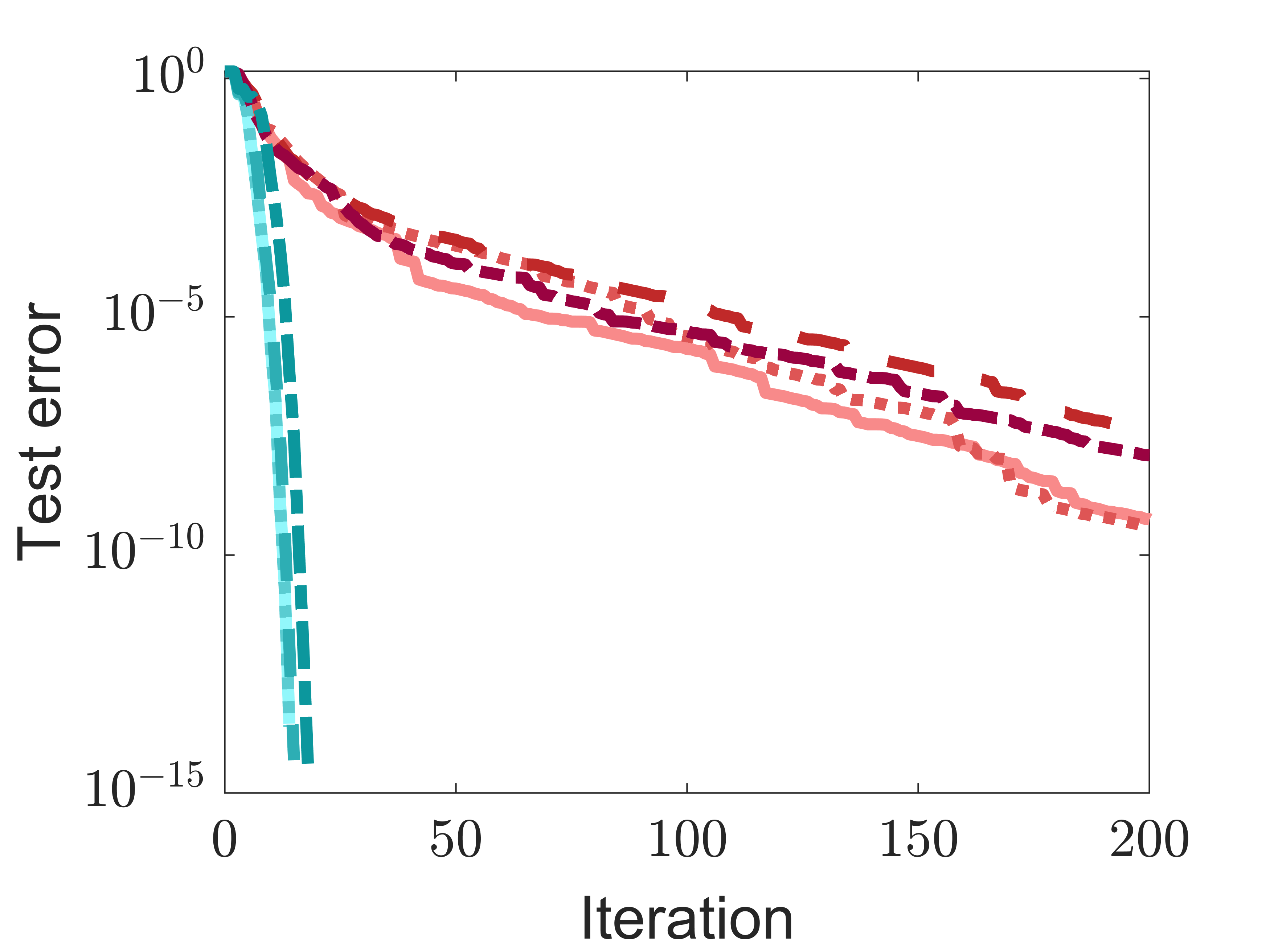
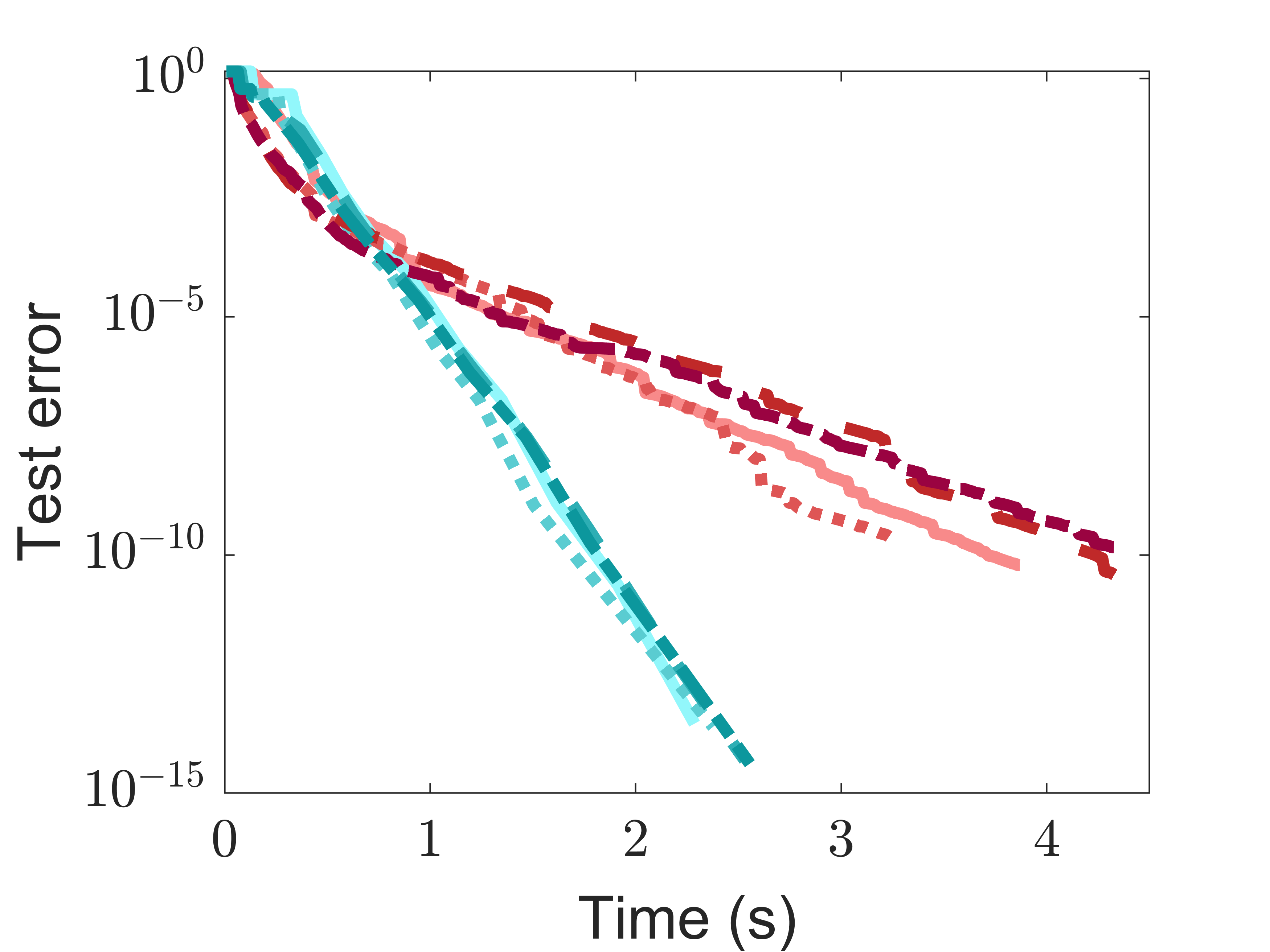
Figure 4: Spherical data fitting problem with the sampling rate $p=0.01$ and the unbiased rank parameter $r=r^{*}=6$.

Test with unbiased rank parameter. The algorithms are evaluated under the unbiased rank parameter $r=r^{*}$. Test errors with the sampling rate $p=0.01$ are reported in Fig. 4. Both RGD and RTR methods show robustness concerning the parameter $\omega$ by successfully recovering the underlying low-rank matrix $A\in\mathrm{Ob}(m,n)$, as evidenced by the test errors.

Test with over-estimated rank parameter. The algorithms are evaluated under over-estimated rank parameters $r=7,8,9,10>r^{*}$ and the sampling rate $p=0.1$. After conducting initial tests, we observe that $\omega=0.5$ for RGD and $\omega=10$ for RTR provide robust performance, for which they will serve as the default settings for all the remaining experiments across this paper. Table 1 reveals that the algorithms reconstruct the true data matrix $A$ across all the selected rank parameters.

Table 1: Spherical data fitting problem with the sampling rate $p=0.1$ and over-estimated rank parameters $r=7,8,9,10>r^{*}$.

Algorithm	$r=7$		$r=8$		$r=9$		$r=10$
	Test err.	Time	Test err.	Time	Test err.	Time	Test err.	Time
$\mathcal{M}_{h}$-RGD	${4.88}\mathrm{e}{-12}$	$11.87$	${5.12}\mathrm{e}{-13}$	$6.55$	${1.11}\mathrm{e}{-12}$	$8.13$	${4.16}\mathrm{e}{-12}$	$16.98$
$\mathcal{M}_{h}$-RTR	${3.34}\mathrm{e}{-15}$	$14.93$	${5.27}\mathrm{e}{-15}$	$8.74$	${5.81}\mathrm{e}{-15}$	$7.19$	${2.14}\mathrm{e}{-15}$	$\phantom{0}7.68$

6.2 Low-rank approximation of graph similarity matrices

Given two graphs $G_{A}$ and $G_{B}$ with $m$ and $n$ nodes, respectively, we denote their adjacency matrices as $A\in\mathbb{R}^{m\times m}$ and $B\in\mathbb{R}^{n\times n}$. For $G_{A}$, $A(i,j)=1$ indicates the existence of an edge from node $i$ to node $j$, while $A(i,j)=0$ otherwise. Moreover, the sets of children and parents of node $i$ in $G_{A}$ are denoted by $C_{A}(i)$ and $P_{A}(i)$, respectively. The same notation applies for the graph $G_{B}$. Adopting a matrix $X\in\mathrm{S}_{\mathrm{F}}(m,n)$ to estimate the similarity between $G_{A}$ and $G_{B}$, Blondel et al. blondel2004measuresimilarity (Blo+04) introduced a linear operator $\mathcal{L}:\,\mathbb{R}^{m\times n}\to\mathbb{R}^{m\times n}$ defined by

$$[\mathcal{L}(X)](i,j):=\sum_{\begin{subarray}{c}s\in C_{A}(i)\\ t\in C_{B}(j)\end{subarray}}A(s,t)+\sum_{\begin{subarray}{c}s\in P_{A}(i)\\ t\in P_{B}(j)\end{subarray}}A(s,t),$$

for $i=1,2,\ldots,m$ and $j=1,2,\ldots,n$, which aggregates the similarity between the neighbors of node $i$ in $G_{A}$ and the neighbors of node $j$ in $G_{B}$. It was proved that the iterates generated by

$$X_{k+1}=\frac{\mathcal{L}(X_{k})}{\|\mathcal{L}(X_{k})\|_{\mathrm{F}}}$$ (6.2)

accumulate at the final similarity matrix $X^{*}$. Afterward, Cason et al. cason2013iterative (CAVD13) showed that solving problem (1.2) yields a matrix of rank at most $r$ to approximate the similarity between $G_{A}$ and $G_{B}$.

In light of the developments in this paper, we address the following problem,

$$\min_{x\in\mathcal{M}_{h}}\ \ -\mathrm{tr}\left({\phi(x)^{\top}\mathcal{L}\circ\mathcal{L}(\phi(x))}\right),$$ (6.3)

with the rank parameter $r$ and the associated manifold $\mathcal{H}=\mathrm{S}_{\mathrm{F}}(m,n)$; and then map the solution $x\in\mathcal{M}_{h}$ to $\phi(x)\in\mathbb{R}^{m\times n}$ as the approximate similarity matrix.

We carry out RGD and RTR on the proposed $\mathcal{M}_{h}$, and implement the “Iterative method” cason2013iterative (CAVD13) by ourselves as the compared method. We initialize $x_{0}\in\mathcal{M}_{h}$ for our methods and $X_{0}\in\mathbb{R}^{m\times n}$ for the “Iterative method” such that $\phi(x_{0})=X_{0}={{\bm{1}}_{m}{\bm{1}}^{\top}_{n}}/{\|{\bm{1}}_{m}{\bm{1}}^{\top}_{n}\|_{\mathrm{F}}}$, where the subscript denotes the length of the all-one vector. The performance is assessed based on the relative errors, ${\|\phi(x)-X^{*}\|_{\mathrm{F}}}/{\|X^{*}\|_{\mathrm{F}}}$ and ${\|X-X^{*}\|_{\mathrm{F}}}/{\|X^{*}\|_{\mathrm{F}}}$, where $X^{*}$, as the ground-truth similarity matrix, is obtained by applying the update rule (6.2) iteratively. The algorithm is terminated if the relative error achieves $10^{-6}$ or the iteration exceeds $200$. We consider two scenarios: the solution $X^{*}$ is low-rank or full-rank.

Test on low-rank solution. We construct $G_{A}$ of $m=2000$ vertices, which form a single cycle with all the edges oriented in the same direction. The graph $G_{B}$ is generated following the binomial random graph model where each edge is included in the graph with the probability $p=0.0005$. In this manner, the similarity matrix $X^{*}$ has the rank $r^{*}=1$, as proved by blondel2004measuresimilarity (Blo+04). We test the method with various rank parameters $r=1,10,50,100$. The results in Fig.  5 show that our method, which is proposed for solving the general problem (P), successfully recovers the true similarity matrix across all settings, exhibiting robustness to the rank parameter. Furthermore, its performance is comparable to the “Iterative method”.

Figure 5: Graph similarity measuring problem when the solution is low-rank. Left: test with the unbiased rank parameter $r=r^{*}=1$; Right: test with over-estimated rank parameters $r=10,50,100>r^{*}$.

Test on full-rank solution. We set $m=n$ and generate both $G_{A}$ and $G_{B}$ following the binomial random graph model with $p=10/m$, which means the average number of outgoing edges of a node is $10$. It is observed from Table 2 that the solution $X^{*}$ is full-rank. Numerical results of “$\mathcal{M}_{h}$-RTR” are presented for various problem dimensions and rank parameters. Specifically, given a small rank $r$, the method produces a decent low-rank approximation of $X^{*}$, and it recovers the true similarity matrix effectively as $r$ approaches the full rank.

Table 2: Graph similarity measuring problem when the solution is full-rank.

Dimension $m$	$r=10\%\times m$		$r=50\%\times m$		$r=75\%\times m$		$r=100\%\times m$
	Rel. err.	Iter.	Rel. err.	Iter.	Rel. err.	Iter.	Rel. err.	Iter.
$200$	${7.82}\mathrm{e}{-7}$	$38$	${1.25}\mathrm{e}{-7}$	$31$	${4.76}\mathrm{e}{-8}$	$26$	${1.43}\mathrm{e}{-11}$	$4$
$400$	${8.23}\mathrm{e}{-7}$	$32$	${1.85}\mathrm{e}{-7}$	$30$	${5.92}\mathrm{e}{-8}$	$26$	${1.07}\mathrm{e}{-11}$	$5$
$600$	${7.61}\mathrm{e}{-8}$	$39$	${5.73}\mathrm{e}{-7}$	$27$	${3.12}\mathrm{e}{-7}$	$28$	${8.71}\mathrm{e}{-12}$	$5$
$800$	${4.82}\mathrm{e}{-7}$	$37$	${5.79}\mathrm{e}{-7}$	$28$	${1.45}\mathrm{e}{-7}$	$21$	${9.31}\mathrm{e}{-12}$	$5$
$1000$	${9.98}\mathrm{e}{-7}$	$37$	${7.13}\mathrm{e}{-7}$	$31$	${3.85}\mathrm{e}{-7}$	$28$	${8.02}\mathrm{e}{-12}$	$5$

6.3 Synchronization problem

Synchronization refers to the problem of determining absolute rotations in $\mathrm{SO}(3):=\{R\in\mathcal{O}(3):\,\det(R)=1\}$ with respect to a shared coordinate system, employing the relative rotation measurements. Concretely, given $n$ cameras and a set of relative rotations $\{\hat{R}_{ij}:(i,j)\in\mathscr{E}\}$, the element $\hat{R}_{ij}$ measures the orientation difference between the $i$-th and $j$-th cameras sharing overlapping view fields. The objective is to reconstruct the absolute rotations $\{R_{i}\}_{i=1}^{n}$ defining the individual orientations of the cameras such that $\hat{R}_{ij}\approx R_{j}R_{i}^{\top}$.

The synchronization problem enjoys an SDP relaxation wang2013rotationsynchronization (WS13), and in view of the reformulation (1.4) in this paper, we consider

$$\min_{x\in\mathcal{M}_{h}}\bar{f}(x)=\langle C,\phi(x)\phi(x)^{\top}\rangle,$$ (6.4)

where the associated $\mathcal{H}=\mathrm{St}(3n,3)^{n}$, the rank parameter for $\mathcal{M}_{h}$ is $r=3$, and the measurement matrix $C\in\mathbb{R}^{3n\times 3n}$ is defined by $C_{ij}=\hat{R}_{ij}^{\top}$ for $(i,j)\in\mathscr{E}$, and $C_{ij}=0$ otherwise. To recover rotations $\{R_{i}\}_{i=1}^{n}$ from the solution $x\in\mathcal{M}_{h}$ of problem (6.4), we utilize the representation $(H,V)$. In detail, noticing that $H=[H^{1}\,H^{2}\,\ldots\,H^{n}]^{\top}\in\mathrm{St}(3n,3)$, which implies all the $3\times 3$ blocks $H^{i}$ are orthogonal, we can extract them as the desired rotations, i.e., letting $R_{i}=(H^{i})^{\top}$, provided their determinants are positive. Note that $\mathrm{SO}(3)$ is a connected component of $\mathcal{O}(3)$ and the adopted retractions on $\mathcal{M}_{h}$ are continuous. Therefore, algorithms on $\mathcal{M}_{h}$ initialized with $H^{i}\in\mathrm{SO}(3)$ $(i=1,2,\ldots,n)$ will always generate iterates $x_{k}$ capable of producing $n$ rotations.

The “Stanford bunny” and the “Spotted cow” datasets are employed for our test; see Fig. 6. In preparation, we randomly generate $360$ camera positions around the original mesh. For each camera, points in the visible portion are sampled to simulate point cloud scanning. Running the automatic Iterative Closest Point algorithm rusinkiewicz2001ICP (RL01), we obtain $1858$ and $1883$ relative rotations for “Stanford bunny” and “Spotted cow”, respectively. The algorithm “$\mathcal{M}_{h}$-RTR” with $\omega=10$ is carried out and it is terminated if the Riemannian gradient satisfies $\|\nabla_{\mathcal{M}_{h}}\bar{f}(x_{k})\|\leq 10^{-13}$. For the initial guess $x_{0}\in\mathcal{M}_{h}$ represented by $(H_{0},V_{0})$, $H_{0}=[H^{1}_{0}\,H^{2}_{0}\,\ldots\,H^{n}_{0}]^{\top}$ is generated by randomly sampling $H^{i}_{0}$ on $\mathrm{SO}(3)$, and $V_{0}$ is randomly generated on $\mathrm{St}(3n,3)$.

The reconstructed point clouds of the two 3D models are visualized in Fig. 6, and the errors are quantified in Fig. 7. The results demonstrate decent reconstruction quality both visually and numerically, validating the effectiveness of the proposed approach on $\mathcal{M}_{h}$ for solving problem (6.4).

​​​​​​​​

​​​​

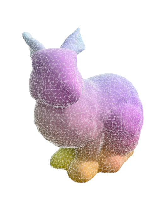
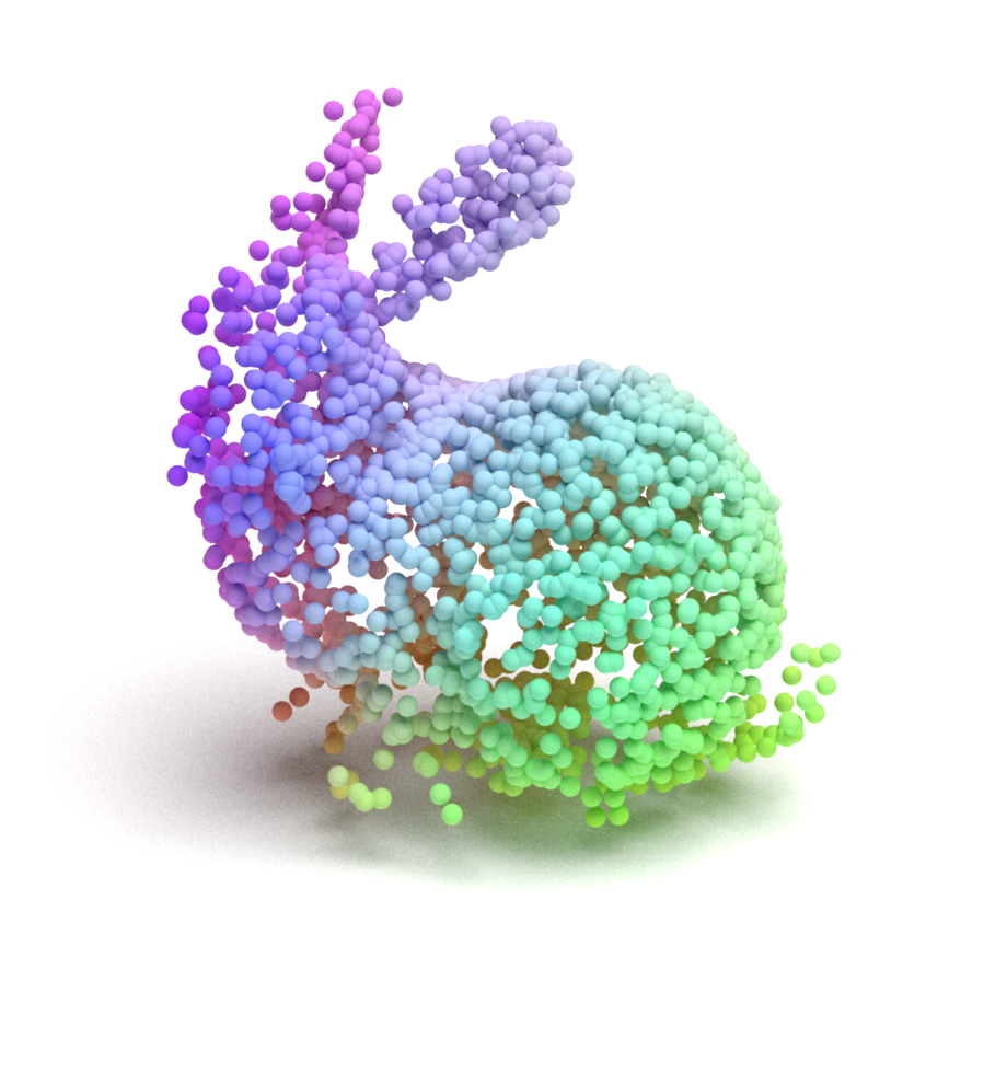
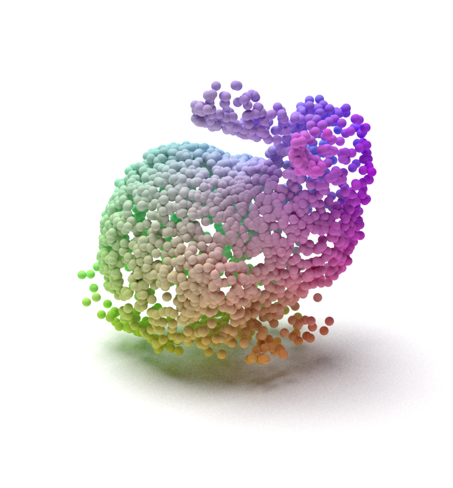
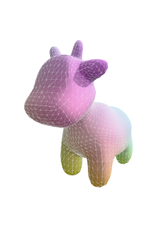
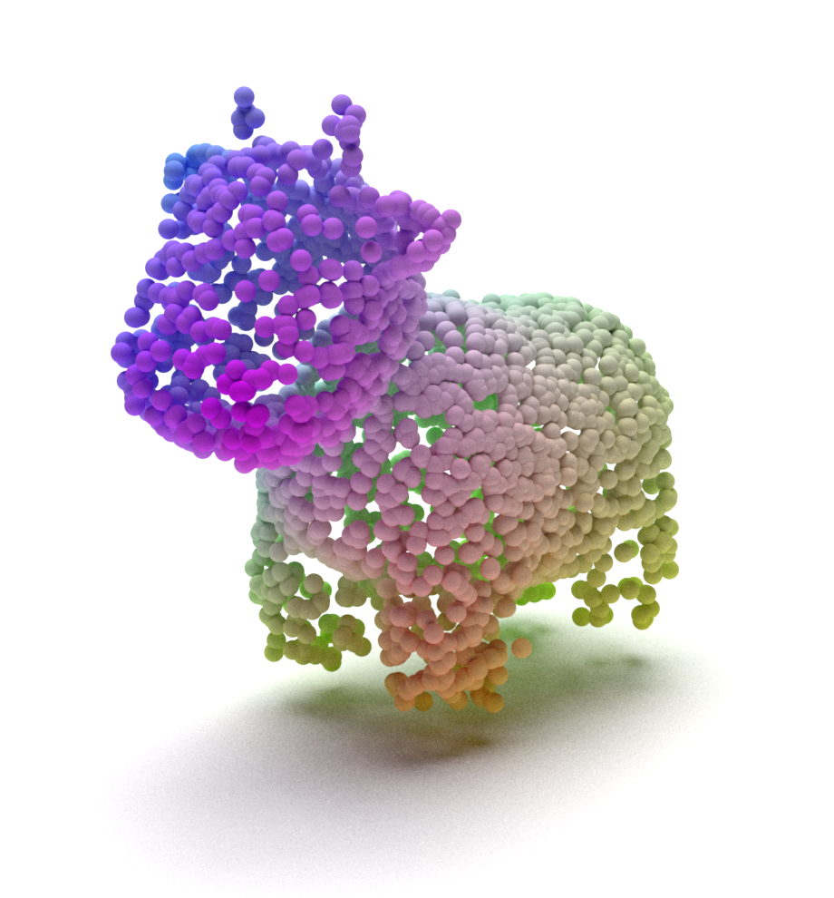
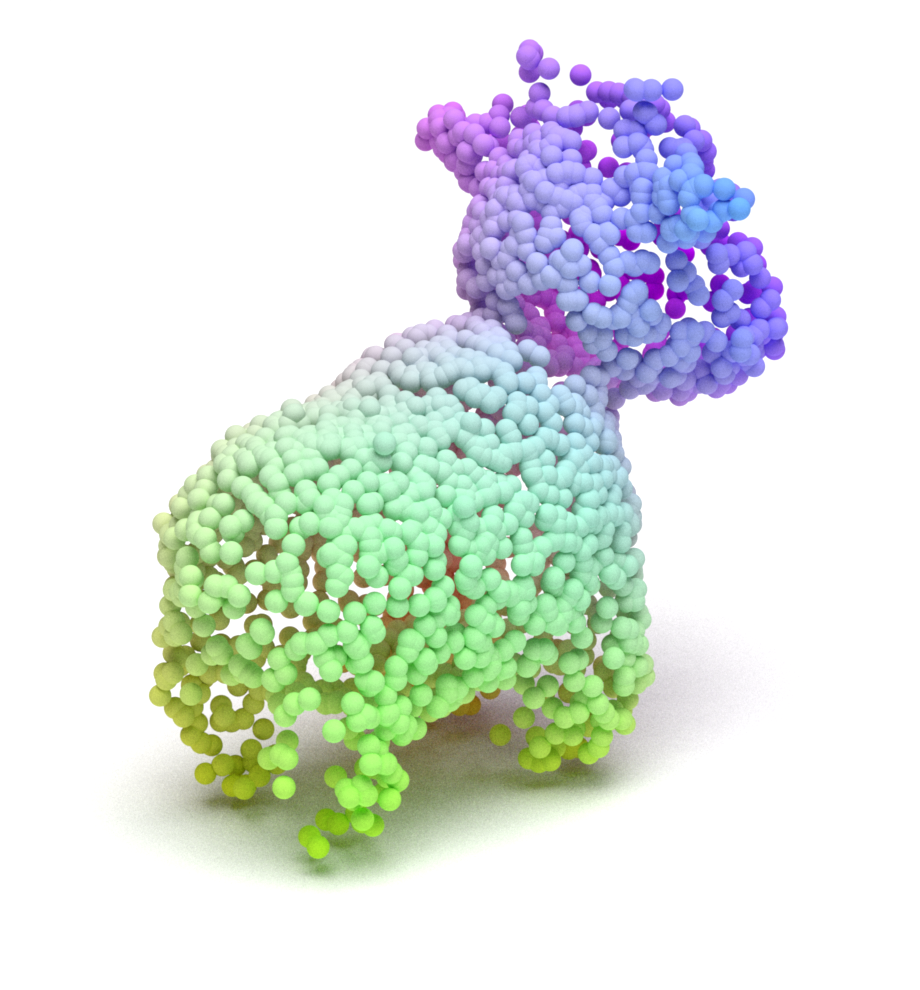
Figure 6: Visualization of “Stanford bunny” and “Spotted cow” in the synchronization problem. Left: original meshes; Middle: front view of the reconstructed point clouds; Right: back view of the reconstructed point clouds.

Figure 7: Reconstructed errors in the synchronization problem, which are evaluated by $\|R_{i}R_{j}^{\top}-\hat{R}_{ij}\|_{\mathrm{F}}$ for $(i,j)$ pairs. The measurements are sparse since only around $1800$ relative rotations are provided for $360$ three-dimensional scans.

6.4 State compression of a city-wide Markov process

we consider the following problem with the associated $\mathcal{H}=\mathrm{Ob}(\left|{\mathcal{S}}\right|,\left|{\mathcal{S}}\right|)$,

$$\min_{x\in\mathcal{M}_{h}}\ \ \frac{1}{2}\|\phi(x)\odot\phi(x)-\hat{\mathrm{P}}\|^{2}_{\mathrm{F}}$$ (6.5)

as a parameterized counterpart of (1.5), to examine the low-rankness of the Manhattan transportation network. The experiment is based on a real-life dataset of $1.1\times 10^{7}$ NYC Yellow cab trips in January 2016 TLC2017 ((TL17), where each entry includes the pick-up and drop-off locations of one trip. We assume that taxi transitions are nearly memoryless and, therefore, characterize the transportation dynamics as a Markov process. In this view, the map is discretized such that locations in the same grid cell are aggregated into a single state, and the recorded trips are seen as transitions between states.

The grid is of the size $0.001^{\circ}\times 0.001^{\circ}$, and states falling outside the region of $80.07^{\circ}\mathrm{W}$ to $60.92^{\circ}\mathrm{W}$ and $30.69^{\circ}\mathrm{N}$ to $50.85^{\circ}\mathrm{N}$ or those with an occurrence frequency below $10^{-4}$ are excluded. Consequently, we collect $2017$ valid states $\mathcal{S}=\{1,2,\ldots,{2017}\}$, and about $7.5\times 10^{6}$ transition indexed by $\left({s^{\text{pickup}}_{t},s^{\text{dropoff}}_{t}}\right)$ with $t=1,2,\ldots,T$. The empirical probability matrix is constructed by

$$\hat{\mathrm{P}}(i,j)=\frac{\sum_{t=1}^{T}\mathbb{I}\left({s^{\text{pickup}}_{t}=i,s^{\text{dropoff}}_{t}=j}\right)}{\sum_{t}^{T}\mathbb{I}\left({s^{\text{pickup}}_{t}=i}\right)},\ \ \text{for}\ \ i,j\in\mathcal{S},$$

where $\mathbb{I}$ is the indicator function of an event, $1$ for happening and $0$ for otherwise.

We implement “$\mathcal{M}_{h}$-RGD” with $\omega=0.5$ to address (6.5), running for $K=500$ iterations to obtain $x_{K}$ represented by $(H_{K},V_{K})\in\mathrm{Ob}(m,r)\times\mathrm{St}(n,r)$. Each row of $H_{K}$ is then treated as a feature vector corresponding to a state, and the MATLAB function kmeans is used to cluster $\mathcal{S}$ based on these features, where the number of clusters is set equal to the rank parameter $r$. In Fig. 8, the clustering results are visualized via Google Maps, showing that the partition based on our approach agrees well with the geometry of this region.

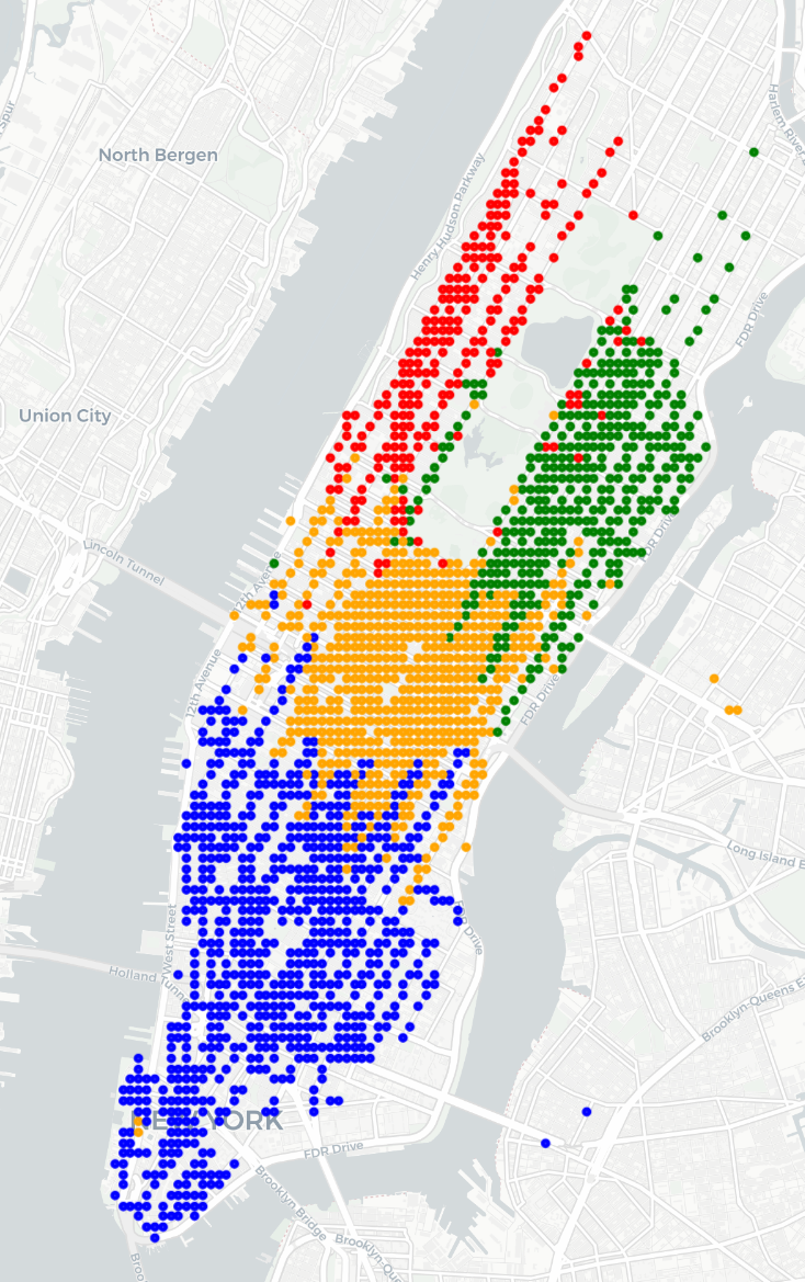
$r=4$

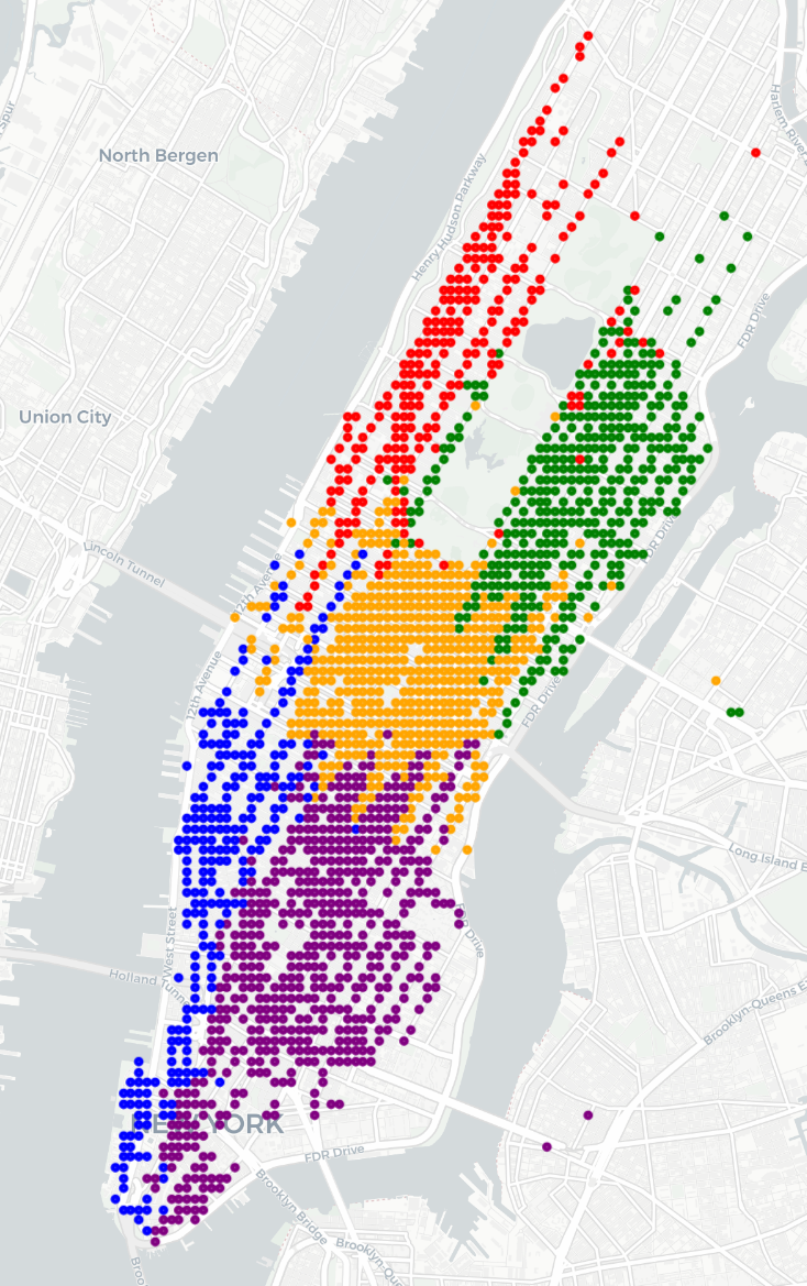
$r=5$

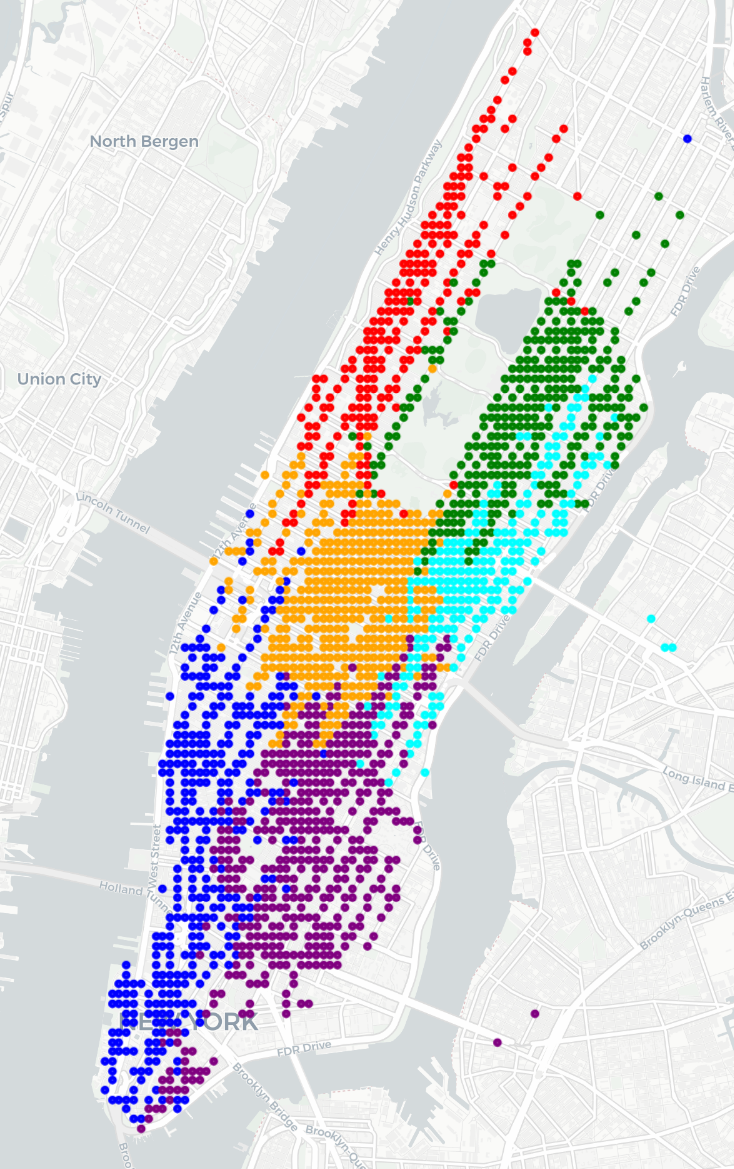
$r=6$

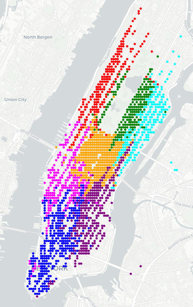
$r=7$

Figure 8: State compression of the Markov process: partition of the Manhattan transportation network.

6.5 Low-rank reinforcement learning

Recalling the proposed model (1.6), we next turn to the following problem

$$\min_{x\in\mathcal{M}_{h}}-J(\pi(\phi(x))),$$ (6.6)

which seeks an optimal low-rank policy. In this problem, $\mathcal{M}_{h}$ is the associated parameterization of $\mathbb{R}_{\leq r}^{\left|{\mathcal{S}}\right|\times\left|{\mathcal{A}}\right|}\cap\mathrm{Ob}(\left|{\mathcal{S}}\right|,\left|{\mathcal{A}}\right|)$. The policy gradient $\nabla J$ can be derived via existing RL theory sutton2018RL (SB18), and its Riemannian counterpart on $\mathcal{M}_{h}$ follows from the formula (5.1). Implementing RGD to solve (6.6) is thus termed the low-rank Riemannian policy gradient (LRRPG) method.

We compare the proposed LRRPG with Q-learning and REINFORCE sutton2018RL (SB18), both of which address RL tasks without exploiting low-rank structures in the environment. Specifically, REINFORCE updates the policy $\pi\in\mathbb{R}^{\left|{\mathcal{S}}\right|\times\left|{\mathcal{A}}\right|}$ based on the policy gradient. Moreover, Q-learning maintains a variable $Q\in\mathbb{R}^{\left|{\mathcal{S}}\right|\times\left|{\mathcal{A}}\right|}$ to estimate the optimal expected accumulative reward conditioned on state-action pairs, and then recover the policy by greedily picking the action with the maximal reward in each state. As summarized in Table 3, LRRPG requires far fewer parameters than the compared methods, thereby mitigating both the memory and computational burdens.

We test on two RL environments of the toolkit OpenAI Gym brockman2016Gym (Bro+16)—“pendulum” and “mountain car”—illustrated in Fig. 9. The evaluation is based on the timestep, which counts the agent’s interaction with the environment, and we report the cumulative reward and the episode’s length as performance metrics. In the implementation, the learning rates for each algorithm are optimally chosen from $\{5\times 10^{i}\mid i=-3,-2,-1,0,1\}$ in “pendulum” and $\{3\times 10^{i}\mid i=-4,-3,-2,-1,0\}$ in “mountain car”. Further details and numerical results are discussed below.

Figure 9: Illustration of RL environments. Left: a pendulum attached at one end to a fixed point, with the other end being free; Right: a car stuck in the sinusoidal valley, with the flag on top of the right hill being the destination.

Pendulum. In this scenario, the agent endeavors to keep an inverted pendulum upright by applying torque to its free end. The problem has two continuous state coordinates (angle and angular velocity) and one continuous action coordinate (torque), necessitating discretization of the state and action spaces. Specifically, by uniformly discretizing the Cartesian product of state coordinates, we generate a finite state space containing $\left|{\mathcal{S}}\right|=2121$ elements. Similar discretization on the action coordinate yields $\left|{\mathcal{A}}\right|=41$. Moreover, a multi-objective $\text{reward}=-(\text{angle}^{2}+0.1\times\text{velocity}^{2}+0.001\times\text{torque}^{2})$ is used, which promotes the pendulum to be upright and encourages small exerted action. The discount factor is set to $\gamma=0.9$. The episode is truncated if the pendulum deviates far away from the upright position, and the maximal episodic life is $100$ timesteps. We adopt the learning rate of $0.05$ for REINFORCE and Q-learning, and $0.005$ for LRRPG.

Parameter efficiency and convergence curves are reported in Table 3 and Fig. 10, showing that in this case, LRRPG achieves the optimal reward and the maximal balanced time faster than REINFORCE. Additionally, the performance of LRRPG is on par with the baseline Q-learning. Increasing the rank enhances initial training, but the influence on the final result is small.

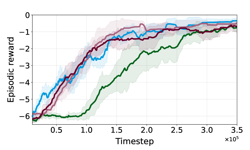
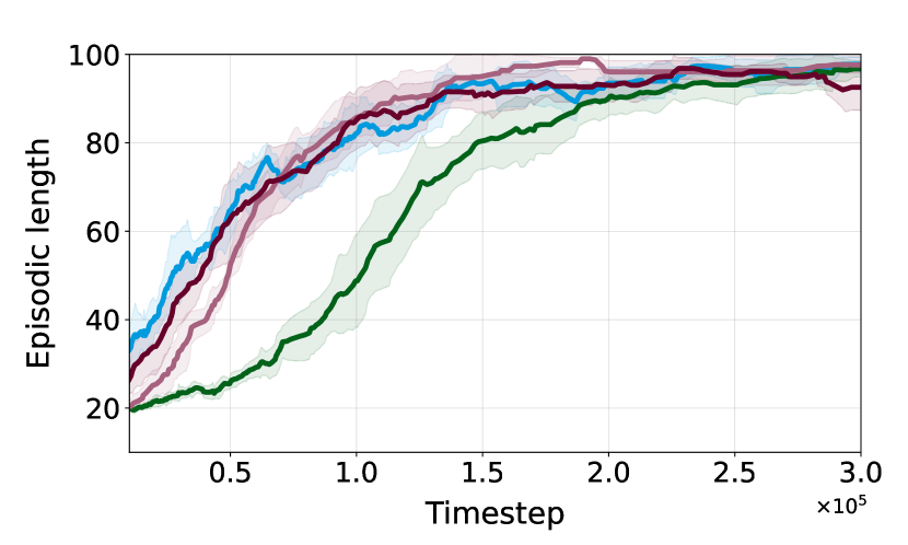
Figure 10: Comparison of the RL algorithms in “pendulum”. The running average over 10 consecutive episodes is adopted for the presentation, and results are averaged over $10$ seeds. A longer episodic length suggests that the agent is more proficient at balancing the pendulum.

Table 3: Parameter efficiency of the proposed method across two environments. The ratio of storage is defined as $\rho_{\textit{storage}}:=\text{Parameters}/\left|{\mathcal{S}}\right|\left|{\mathcal{A}}\right|$. Episodic rewards are averaged over $10$ runs. The results are reported after $0.3$M and $12$M timesteps in the “pendulum” and “mountain car”, respectively.

Algorithm	Pendulum			Mountain car
	Parameters	$\rho_{\text{storage}}$	Reward	Parameters	$\rho_{\textit{storage}}$	Reward
REINFORCE	$86,961$	$1.00$	$-0.94$	$582,096$	$1.00$	$96.99$
Q-learning	$86,961$	$1.00$	$-0.75$	$582,096$	$1.00$	$83.95$
LRRPG ($r=5$)	$10,810$	$0.12$	$-0.73$	$\phantom{0}15,485$	$0.03$	$88.31$
LRRPG ($r=10$)	$21,620$	$0.25$	$-0.58$	$\phantom{0}30,970$	$0.05$	$86.44$
LRRPG ($r=15$)	$32,430$	$0.37$	$-0.83$	$\phantom{0}46,455$	$0.08$	$78.23$

Mountain car. In this environment, the decision process involves applying an appropriate directional force to help the car, initially stuck at the bottom of the valley, reach the goal state on top of the right mountain. A negative reward of $-0.1\times\text{force}^{2}$ is received at each timestep to penalize for taking actions of large magnitude. As an incentive, a positive reward of $+100$ will be added if the car reaches the goal. We discretize the original continuous state and action spaces to obtain finite ones with $\left|{\mathcal{S}}\right|=2896$ and $\left|{\mathcal{S}}\right|=201$. The discount factor is set to $\gamma=0.99$, and the maximal episodic life is $1000$ timesteps. The learning rates are chosen as $0.3$ for Q-learning, $0.03$ for REINFORCE, and $0.0003$ for LRRPG.

Although the low-rank method slightly lowers the final reward, it significantly improves storage efficiency while maintaining overall performance comparable to Q-learning and REINFORCE, as illustrated by Fig. 11. Specifically, with ${r=5}$, LRRPG uses parameters amounting to only $2.66\%$ of the environment size $\left|{\mathcal{S}}\right|\times\left|{\mathcal{A}}\right|$, yet it still learns a low-rank policy that successfully drives the car to the mountaintop; see Table 3 for detailed comparison across different rank parameters.

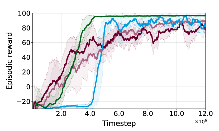
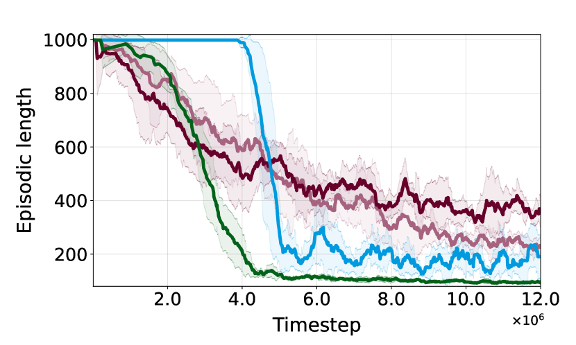
Figure 11: Comparison of the RL algorithms in “mountain car”. The running average over 10 consecutive episodes is adopted for the presentation, and results are averaged over $10$ seeds. Shorter episodes mean the agent drives the car to its destination faster.

6.6 Low-rank neural network with weight normalization

To validate the effectiveness of combining the weight normalization technique (WN) and low-rank compression (LR) on neural networks, we solve the following parameterized version of (1.7),

$$\min_{x_{i}\in\mathcal{M}_{h_{i}},\,g_{i}}\ f(\{\phi(x_{i}),g_{i}\}_{i=1}^{l}).$$ (6.7)

The proposed approach is tested on two benchmark classification datasets, MNIST lecun1998mnist (LeC+98) and CIFAR-10 krizhevsky2009CIFAR (Kri09).

Table 4: Neural network training with different parameterizations.

Model​​​	​​​Weight norm.​​​	​​Low rank​	​Net. param.​	Search space​	Remark
Vanilla​​	-	-	$\{W_{i}\}$	$\mathbb{R}^{m_{i}\times n_{i}}$	-
WN	✓	-	$\{X_{i},g_{i}\}$	$\mathrm{Ob}(m_{i},n_{i})\!\times\!\mathbb{R}^{m_{i}}$	-
LR	-	✓	$\{x_{i},g_{i}\}$	$\mathcal{M}_{h_{i}}\!\times\!\mathbb{R}^{m_{i}}\!\!\!$	$h_{i}(\cdot)\equiv 0$
WN+LR​​​	✓	✓	$\{x_{i},g_{i}\}$	$\mathcal{M}_{h_{i}}\times\mathbb{R}^{m_{i}}$	$h_{i}(X_{i})=X_{i}X_{i}^{\top}\!-\!\mathbf{1}$

To assess the respective contributions of WN and LR, as well as their combined effect, we conduct an ablation study that compares the baseline neural network, the network with WN, the network with LR, and the network incorporating both WN and LR. These four models employ different parameterizations of the neural network, as presented in Table 4. Note that if only the low-rank compression is imposed, the model resembles (6.7), but the search space simplifies to $\mathcal{M}_{h_{i}}$ with the associated mapping $h_{i}(\cdot)\equiv 0$. In the implementation, we use the stochastic (Riemannian) gradient descent method in the corresponding search space, assisted with an appropriate momentum. Implementation details and hyper-parameter specifications are provided in Appendix C.

Numerical outcomes are reported in Fig. 12 and Table 5, where the metric flops is defined as floating point operations. Regarding the fully parameterized models, the results verify that imposing WN enhances the performance over the vanilla network. As a counterpart, for the low-rank models, “WN+LR” achieves faster convergence on MNIST and delivers higher accuracy on CIFAR-10 than “LR”. Moreover, as shown in Table 5, although the proposed “WN+LR” trades a small amount of accuracy when classifying CIFAR-10, it offers considerable parameter efficiency and inference acceleration compared to fully parameterized models. In conclusion, the findings reveal that combining weight normalization and low-rank compression presents a promising direction for designing neural networks.

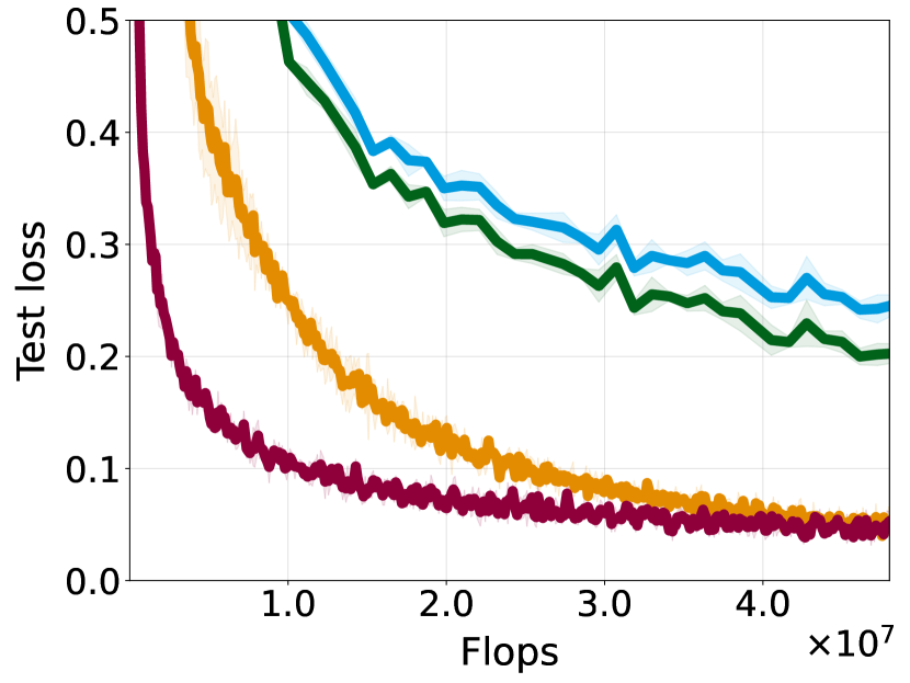
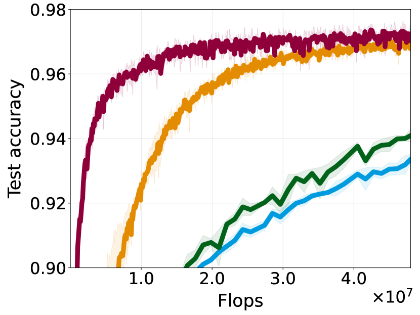
Figure 12: Comparison of the network models on MNIST classification.

Table 5: Comparison among the network models on CIFAR-10 classification. Reported metrics include the number of parameters, storage ratio, flops per inference and their ratio, and the top-1 training/test accuracy.

Algorithm	Parameters	$\rho_{\textit{storage}}$	Infer. flops	$\rho_{\textit{infer}}$	Train. acc. ($\%$)	Test acc. ($\%$)
CNN (vanilla)	$2.62$M	$1.00$	$565.50$M	$1.00$	$\phantom{0}96.67$	$87.80$
CNN (WN)	$2.62$M	$1.00$	$565.50$M	$1.00$	$100.00$	$90.31$
CNN (LR)	$0.38$M	$0.14$	$179.02$M	$0.32$	$\phantom{0}90.01$	$83.07$
CNN (WN+LR)	$0.38$M	$0.14$	$179.02$M	$0.32$	$\phantom{0}95.39$	$87.30$

7 Conclusions and perspectives

In this paper, we propose a space-decoupling framework for optimization problems on bounded-rank matrices with orthogonally invariant constraints. Specifically, we identify the tangent and normal cones of the coupled feasible set. Then, a smooth space-decoupling parametrization $\mathcal{M}_{h}$ is introduced, which reformulates the original nonsmooth problem into a smooth Riemannian optimization problem. Geometric tools for implementing Riemannian algorithms are developed, and our analysis demonstrates the equivalence between the reformulated and original problems. We conclude by offering several comments and outlining potential future directions inspired by this work.

Generalization from right to left invariance. The proposed space-decoupling framework rests on the right orthogonally invariant property of $h$, i.e., $h(XQ)=h(X)$ for all $Q\in\mathcal{O}(n)$. In essence, all results can be generalized to the case when $h(QX)=h(X)$ following from a parallel analysis. For example, the focused decomposition shifts from $X=HV^{\top}$ to $X=UH$, and the constraint in the definition of $\mathcal{M}_{h}$ (see (4.1)) is reversed from $XG=0$ to $GX=0$.

Discussion on the blanket assumption. The smoothness assumption for the mapping $h:\,\mathbb{R}^{m\times n}\rightarrow\mathbb{R}^{q}$ can be relaxed to twice continuous differentiability, while all the corresponding results in this paper remain valid. In fact, the full-rank condition in Assumption 1 corresponds to the linear independence constraint qualification (LICQ) for the constraint $h(X)=0$.

Another parameterization for the feasible region. It is worth noting that by defining the mapping $\psi:\mathbb{R}^{m\times r}\times\mathbb{R}^{n\times r}:(H,V)\mapsto HV^{\top}$, we can derive an alternative parameterization $(\mathcal{H}^{r}\times\mathrm{St}(n,r),\psi)$ in the sense that $\psi(\mathcal{H}^{r}\times\mathrm{St}(n,r))=\mathbb{R}_{\leq r}^{m\times n}\cap\mathcal{H}$, and thus obtain an reformulated problem on $\mathcal{H}^{r}\times\mathrm{St}(n,r)$. Essentially, the equivalence between this Riemannian problem with the original problem (P) has been implied by the proof of Theorem 5.1—similar “$k\Rightarrow 1$” ($k=1,2$) conditions hold true. The construction of geometric tools on the new parameterization mirrors the study of $\mathcal{M}_{h}$, which builds on the theoretical results developed in sections 2 and 3.

Extension of geometric methods on the bounded-rank variety. Theorem 3.1 provides a closed-form characterization for the tangent cone to $\mathbb{R}_{\leq r}^{m\times n}\cap\mathcal{H}$, which exhibits a parallel structure as that to $\mathbb{R}_{\leq r}^{m\times n}$. Notably, $\mathrm{T}_{X}\mathbb{R}_{\leq r}^{m\times n}$ plays a pivotal role in existing retraction-free algorithms schneider2015Lojaconvergence (SU15, OA23, OA24) and the rank-adaptive mechanism gao2022Rieadap (GA22) for optimization on the bounded-rank set. Therefore, these techniques have the potential to be adapted to tackle problem (P), based on the results developed in this work.

Appendix A Riemannian Hessian on $\mathcal{M}_{h}$

In this section, we present the computation of the Riemannian Hessian on $\mathcal{M}_{h}$. The following corollaries will facilitate the computations in Proposition 9.

Corollary 5

Given $X\in\mathbb{R}^{m\times n}$ with a decomposition $X=HV^{\top}$ where $H\in\mathbb{R}^{m\times s}$ and $V\in\mathrm{St}(n,s)$, it holds that, for any $E\in\mathbb{R}^{m\times n}$ and $Y\in\mathbb{R}^{m\times s}$,

$$\mathcal{P}_{\mathrm{T}_{X}\mathcal{H}}(EVV^{\top}) =\mathcal{P}_{\mathrm{T}_{X}\mathcal{H}}(E)VV^{\top},$$ (A.1)

$$\mathcal{P}_{\mathrm{T}_{X}\mathcal{H}}(YV^{\top}) =\left[{\mathcal{P}_{\mathrm{T}_{H}\mathcal{H}^{s}}\left({Y}\right)}\right]V^{\top}.$$ (A.2)

Proof

Applying (2.6) gives the first equality. Moreover, taking $E=YV^{\top}$ in (2.6) confirms the second equality.

According to the computation of the Riemannian Hessian in (5.2), with $(H,V)$ representing $(X,G)\in\mathcal{M}_{h}$, we outline the subsequent quantities associated with $X$,

$$\begin{array}[]{ll}a_{0}(X)=\left({2\omega I+XX^{\top}}\right)^{-1},&\ \ a_{1}(X)=XX^{\top}a_{0}(X),\\ a_{2}(X)=a_{0}(X)X,&\ \ a_{3}(X)=X^{\top}X(2\omega I+X^{\top}X)^{-1}.\end{array}$$ (A.3)

Equivalently, these quantities can be computed via the representation $(H,V)$.

$$\begin{array}[]{ll}a_{0}(X):=\left({2\omega I+HH^{\top}}\right)^{-1},&\ \ a_{1}(X):=HM_{H,\omega}^{-1}H^{\top},\\ a_{2}(X):=HM_{H,\omega}^{-1}V^{\top},&\ \ a_{3}(X):=VM_{H,\omega}^{-1}V^{\top}+\frac{1}{2\omega}(I-VV^{\top}).\end{array}$$ (A.4)

To give $\nabla^{2}_{\mathcal{M}_{h}}\bar{f}(X,G)[\eta,\zeta]$ explicitly, we need to identify $\mathfrak{D}(E,Z)$ as the first step.

Lemma 6

Given $(X,G)\in\mathcal{M}_{h}$ and $(\eta,\zeta)\in\mathrm{T}_{(X,G)}\mathcal{M}_{h}$ with representations $(H,V)$ and $(K,V_{p})$, respectively, we denote $\mathcal{P}_{(X,G)}(E,Z)=(P_{1},P_{2})$ and $\mathfrak{D}(E,Z)=(D_{1},D_{2})$. Then, they can be computed as follows,

$$\begin{cases}P_{1}=\mathcal{P}_{\mathrm{T}_{X}\mathcal{H}}\left({E(I-G)}\right)+a_{1}(X)EG-2\omega a_{2}(X)ZG,\\ P_{2}=2\mathrm{sym}\left({-GE^{\top}a_{2}(X)+2\omega GZa_{3}(X)-GZG}\right),\end{cases}$$

$$\begin{cases}D_{1}=\mathrm{D}\left({\tilde{X}\mapsto\mathcal{P}_{\mathrm{T}_{\tilde{X}}\mathcal{H}}(E(I-G))}\right)(X)[\eta]-\mathcal{P}_{\mathrm{T}_{X}\mathcal{H}}(E\zeta)\\ \quad\quad\,\,\,\,+\,\mathrm{D}a_{1}(X)[\eta]EG+a_{1}(X)E\zeta-2\omega\mathrm{D}a_{2}(X)[\eta]ZG-2\omega a_{2}(X)Z\zeta,\\ D_{2}=2\mathrm{sym}\big{(}-\zeta E^{\top}a_{2}(X)-GE^{\top}\mathrm{D}a_{2}(X)[\eta]+2\omega\zeta Za_{3}(X)\\ \quad\quad\quad\quad\quad\ \ +2\omega GZ\mathrm{D}a_{3}(X)[\eta]-\zeta ZG-GZ\zeta\big{)}.\end{cases}$$

Proof

Incorporate the projection (4.6) into the formula (4.3),

$$P_{1}= \ \mathcal{P}_{\mathrm{T}_{H}\mathcal{H}^{r}}(EV)V^{\top}+HM_{H,\omega}^{-1}(H^{\top}E-2\omega V^{\top}Z)G$$

$$\overset{(i)}{=} \ \mathcal{P}_{\mathrm{T}_{X}\mathcal{H}}\left({E(I-G)}\right)+a_{1}(X)EG-2\omega a_{2}(X)ZG,$$

$$P_{2}= -2\mathrm{sym}\left({G(E^{\top}H-2\omega ZV)M_{H,\omega}^{-1}V^{\top}}\right)$$

$$\overset{(ii)}{=} \ 2\mathrm{sym}\left({-GE^{\top}a_{2}(X)+2\omega GZa_{3}(X)-GZG}\right),$$

where $(i),(ii)$ come from (A.2) and (A.4). Subsequently, taking the derivatives of $P_{i}$ with respect to $(X,G)$ along $(\eta,\zeta)$ yields $D_{i}\,(i=1,2)$.

Finally, we give the proof of Proposition 9 as follows.

Proof

The rule (5.2) guides us to calculate $\mathfrak{D}(\nabla\bar{f}(X,G))$ and $\nabla^{2}\bar{f}(X,G)[\eta,\zeta]$, and then project the sum of them onto $\mathrm{T}_{(X,G)}\mathcal{M}_{h}$ to derive $\nabla^{2}_{\mathcal{M}_{h}}\bar{f}(X,G)[\eta,\zeta]$. To begin with, we conduct the following computations,

$$\mathrm{D}a_{0}(X)[\eta]= -a_{0}(X)(\eta X^{\top}+X\eta^{\top})a_{0}(X),$$ (A.5)

$$\mathrm{D}a_{1}(X)[\eta]= \left({\eta X^{\top}+X\eta^{\top}}\right)a_{0}(X)+XX^{\top}\mathrm{D}a_{0}(X)[\eta],$$

$$\mathrm{D}a_{2}(X)[\eta]= \ \mathrm{D}a_{0}(X)[\eta]X+a_{0}(X)\eta.$$

Taking $(E,Z)=\nabla\bar{f}(X,G)=(\nabla f(X),0)$ in Lemma 6, we obtain $\mathfrak{D}(\nabla\bar{f}(X,G))$ by

$$D_{1}= \ \mathrm{D}\left({\tilde{X}\mapsto\mathcal{P}_{\mathrm{T}_{\tilde{X}}\mathcal{H}}(\nabla f(X)(I-G))}\right)(X)[\eta]-\mathcal{P}_{\mathrm{T}_{X}\mathcal{H}}(\nabla f(X)\zeta)$$

$$+\mathrm{D}a_{1}(X)[\eta]\nabla f(X)G+a_{1}(X)\nabla f(X)\zeta,$$

$$D_{2}= \ 2\mathrm{sym}\left({-\zeta\nabla f(X)^{\top}a_{2}(X)-G\nabla f(X)^{\top}\mathrm{D}a_{2}(X)[\eta]}\right).$$

Additionally, note that $\nabla^{2}\bar{f}(X,G)[\eta,\zeta]=\left({\nabla^{2}f(X)[\eta],0}\right)$. Through the lens of (5.2), it suffices to set $(E,Z)=(D_{1}+\nabla^{2}f(X)[\eta],D_{2})$ in (4.6) to get the representation of $\nabla^{2}_{\mathcal{M}_{h}}\bar{f}(X,G)[\eta,\zeta]$. In detail,

$$\bar{K}=\mathcal{P}_{\mathrm{T}_{H}\mathcal{H}^{r}}\left({\left({D_{1}+\nabla^{2}f(X)[\eta]}\right)V}\right)=\left[{\mathcal{P}_{\mathrm{T}_{X}\mathcal{H}}\left({\left({D_{1}+\nabla^{2}f(X)[\eta]}\right)VV^{\top}}\right)}\right]V,$$ (A.6)

which results from $V\in\mathrm{St}(n,r)$ and (A.2). To simplify the computation, consider the curves $H(t)\in\mathcal{H}^{r}$ and $V(t)\in\mathrm{St}(n,r)$ satisfying $H(0)=H,\,H^{\prime}(0)=K$ and $V(0)=V,\,V^{\prime}(0)=V_{p}$. Moreover, we turn to the differential of the curve $Y(t):=\mathcal{P}_{\mathrm{T}_{\tilde{X}(t)}\mathcal{H}}(\nabla f(X)V(t)V(t)^{\top})$ at $t=0$, where $\tilde{X}(t):=H(t)V^{\top}(t)$. In fact, by (A.1), we have

$$Y(t)=\mathcal{P}_{\mathrm{T}_{\tilde{X}(t)}\mathcal{H}}(\nabla f(X)V(t)V(t)^{\top})=\mathcal{P}_{\mathrm{T}_{\tilde{X}(t)}\mathcal{H}}(\nabla f(X))V(t)V(t)^{\top},$$

and thus the differential can be computed from the following two ways,

$$Y^{\prime}(0)=\mathrm{D}\left({\tilde{X}\mapsto\mathcal{P}_{\mathrm{T}_{\tilde{X}}\mathcal{H}}(\nabla f(X)VV^{\top})}\right)(X)[\eta]-\mathcal{P}_{\mathrm{T}_{{X}}\mathcal{H}}(\nabla f(X)\zeta)$$ (A.7)

$$Y^{\prime}(0)=\mathrm{D}\left({\tilde{X}\mapsto\mathcal{P}_{\mathrm{T}_{\tilde{X}}\mathcal{H}}(\nabla f(X))}\right)(X)[\eta]VV^{\top}-\mathcal{P}_{\mathrm{T}_{{X}}\mathcal{H}}(\nabla f(X))\zeta$$ (A.8)

Comparing the above two expressions, applying Proposition 3, and considering the Riemannian Hessian of $X\mapsto f(X)$ on $\mathcal{H}$, we find

$$\,\mathcal{P}_{\mathrm{T}_{X}\mathcal{H}}\left({\left[{\mathrm{D}\left({\tilde{X}\mapsto\mathcal{P}_{\mathrm{T}_{\tilde{X}}\mathcal{H}}(\nabla f(X)VV^{\top})}\right)(X)[\eta]+\nabla^{2}f(X)[\eta]}\right]VV^{\top}}\right)$$

$$= \ \mathcal{P}_{\mathrm{T}_{X}\mathcal{H}}\left({{\mathrm{D}\left({\tilde{X}\mapsto\mathcal{P}_{\mathrm{T}_{\tilde{X}}\mathcal{H}}(\nabla f(X))}\right)(X)[\eta]+\nabla^{2}f(X)[\eta]}}\right)VV^{\top}$$

$$= \ \nabla^{2}_{\mathcal{H}}f(X)[\eta]VV^{\top}.$$ (A.9)

Substituting the expression of $D_{1}$, the result (A.9), and $\zeta=-V_{p}V^{\top}-VV^{\top}_{p}$ into (A.6), we obtain

$$\bar{K}=\nabla^{2}_{\mathcal{H}}f(X)[\eta]V+\mathcal{P}_{\mathrm{T}_{H}{\mathcal{H}^{r}}}\left({\nabla f(X)V_{p}-a_{1}(X)\nabla f(X)V_{p}}\right),$$

and expand $a_{1}(X)$ to achieve the expression of $\bar{K}$ in (5.3).

By (4.6), we next address the term

$$\bar{V}_{p}=\ G\left({(D_{1}+\nabla^{2}f(X)[\eta])^{\top}H-2\omega D_{2}V}\right)M^{-1}_{H,\omega}.$$ (A.10)

According to expressions (A.7) and (A.8), it follows that

$$\mathrm{D}\left({\tilde{X}\mapsto\mathcal{P}_{\mathrm{T}_{\tilde{X}}\mathcal{H}}(\nabla f(X)VV^{\top}}\right)(X)[\eta]G= \left({\mathcal{P}_{\mathrm{T}_{{X}}\mathcal{H}}(\nabla f(X)\zeta)-\mathcal{P}_{\mathrm{T}_{{X}}\mathcal{H}}(\nabla f(X))\zeta}\right)G$$

$$= \left({-\nabla f(X)VV^{\top}_{p}+\mathcal{P}_{\mathrm{T}_{{X}}\mathcal{H}}(\nabla f(X))VV^{\top}_{p}}\right)G$$

$$= -\mathcal{P}_{\mathrm{N}_{H}\mathcal{H}^{r}}(\nabla f(X)V)V^{\top}_{p},$$ (A.11)

where the second and last equalities hold from $\mathcal{P}_{\mathrm{T}_{X}\mathcal{H}}(\nabla f(X)\zeta)G=-\nabla f(X)VV_{p}^{\top}$ and Proposition 3, respectively. Substituting the expressions of $D_{1}$, $D_{2}$, and (A.11) into (A.10) yields

$$\bar{V}_{p}{=} -GV_{p}[\mathcal{P}_{\mathrm{N}_{H}\mathcal{H}^{r}}(\nabla f(X)V)]^{\top}HM^{-1}_{H,\omega}+G\nabla f(X)^{\top}\left({\mathrm{D}a_{1}(X)[\eta]H+2\omega Da_{2}(X)[\eta]V}\right)M^{-1}_{H,\omega}$$

$$+G(\nabla^{2}f(X)[\eta])^{\top}HM^{-1}_{H,\omega}+G\zeta\nabla f(X)^{\top}\left({a_{1}(X)H-H+2\omega a_{2}(X)V}\right)M^{-1}_{H,\omega}$$

$${=} -GV_{p}[\mathcal{P}_{\mathrm{N}_{H}\mathcal{H}^{r}}(\nabla f(X)V)]^{\top}HM^{-1}_{H,\omega}+G\nabla f(X)^{\top}(I-HM^{-1}_{H,\omega}H^{\top})KM^{-1}_{H,\omega}$$

$$+G(\nabla^{2}f(X)[\eta])^{\top}HM^{-1}_{H,\omega},$$

where we employ (A.3), (A.4) and (A.5) to get the last equality.

Appendix B Proof of Proposition 11

Proof

The first step is to verify the map $\mathrm{R}$ is well-defined. To see this, we consider another representation $\left({H_{0},V_{0}}\right)$ for $(X,G)$ and denote the induced quantities with a zero in the subscript. The proof of Proposition 10 shows $\left({H_{0},V_{0}}\right)=(HQ,VQ)$ and $(K_{0},V_{p,0})=(KQ,V_{p}Q)$ for some $Q\in\mathcal{O}(r)$. Similarly, it holds that $L_{0}=LQ$ and $W_{0}=WQ$, due to the constructions of $L$ and $W$. Consequently, the value of $\mathrm{R}_{(X,G)}(\eta,\zeta)$ is independent of the choice of representations since $[\mathcal{P}_{\mathcal{H}^{r}}\left({(X+\eta)W}\right)]W^{\top}=[\mathcal{P}_{\mathcal{H}^{r}}\left({(X+\eta)W_{0}}\right)]W_{0}^{\top}$ and $WW^{\top}=W_{0}W_{0}^{\top}$.

Now, it remains to show $\mathrm{R}$ is second-order, for which we outline the following curves in preparation,

$$L(t):=V+tV_{p}-t^{2}V_{p}K^{\top}HM^{-1}_{H,\omega},\ Z(t):=(L(t)^{\top}L(t))^{-1/2},\ W(t):=L(t)Z(t),$$

$$\beta(t):=(X+t\eta)W(t),\ X(t):=\left[{\mathcal{P}_{\mathcal{H}^{r}}\left({\beta(t)}\right)}\right]W(t)^{\top},\ G(t):=I-W(t)W(t)^{\top},$$

$$\gamma(t):=\left({X(t),G(t)}\right)=\mathrm{R}_{(X,G)}(t\eta,t\zeta).$$

Take the derivative on both sides of the equation $Z(t)^{2}=(L(t)^{\top}L(t))^{-1}$,

$$Z^{\prime}(t)Z(t)+Z(t)Z^{\prime}(t)=-Z(t)^{2}\left({L^{\prime}(t)^{\top}L(t)+L(t)^{\top}L^{\prime}(t)}\right)Z(t)^{2}.$$ (B.1)

Setting $t=0$ and substituting $Z(0)=I,\,L(0)^{\top}L^{\prime}(0)=0$ lead to $Z^{\prime}(0)=0$. Identifying the differential of $\mathcal{P}_{\mathcal{H}^{r}}$ at $H$ as $\mathcal{P}_{\mathrm{T}_{H}\mathcal{H}^{r}}$ (see (absil2012projectionlike, AM12, Lemma 4)) gives

$$X^{\prime}(0)=\mathcal{P}_{\mathrm{T}_{H}\mathcal{H}^{r}}(\beta^{\prime}(0))W(0)^{\top}+\mathcal{P}_{\mathcal{H}^{r}}(H)W^{\prime}(0)^{\top}=KV^{\top}+HV_{p}^{\top}.$$

By evaluating the equality $G^{\prime}(t)=-W^{\prime}(t)W(t)^{\top}-W(t)W^{\prime}(t)^{\top}$ at $t=0$, we have

$$\begin{cases}\gamma(0)=(X(0),G(0))=(X,G),\\ \gamma^{\prime}(0)=\left({X^{\prime}(0),G^{\prime}(0)}\right)=\left({KV^{\top}+HV^{\top}_{p},-V_{p}V^{\top}-VV^{\top}_{p}}\right)=(\eta,\zeta),\end{cases}$$

which verifies $\mathrm{R}$ is a retraction. To proceed, define the curve $\alpha(t):=\mathcal{P}_{\mathcal{H}^{r}}(\beta(t))$ to be the projection of $\beta(t)$ onto $\mathcal{H}^{r}$, and the operator $\mathcal{P}(t)$ to be the projection onto $\mathrm{T}_{\alpha(t)}\mathcal{H}^{r}$, which turns out to be a smooth and linear operator. Notice that $\beta(t)-\alpha(t)$ is orthogonal to $\mathrm{T}_{\alpha(t)}\mathcal{H}^{r}$, i.e., $\mathcal{P}(t)(\beta(t)-\alpha(t))=0$. Differentiate this equation twice,

$$\ddot{\mathcal{P}}(t)(\beta(t)-\alpha(t))+2\mathcal{P}^{\prime}(t)(\beta^{\prime}(t)-\alpha^{\prime}(t))+\mathcal{P}(t)(\ddot{\beta}(t)-\ddot{\alpha}(t))=0.$$

The observation $\alpha(0)=\beta(0)=H$ and $\alpha^{\prime}(0)=\beta^{\prime}(0)=K$ gives

$$\mathcal{P}_{\mathrm{T}_{H}\mathcal{H}^{r}}(\ddot{\alpha}(0))=\mathcal{P}_{\mathrm{T}_{H}\mathcal{H}^{r}}(\ddot{\beta}(0)).$$ (B.2)

Subsequently, we differentiate (B.1) at $t=0$ to obtain $\ddot{Z}(0)=-V_{p}^{\top}V_{p}$ and

$$\ddot{W}(0)=\ddot{L}(0)Z(0)+2L^{\prime}(0)Z^{\prime}(0)+L(0)\ddot{Z}(0)=-2V_{p}K^{\top}HM^{-1}_{H,\omega}-VV_{p}^{\top}V_{p}.$$

Then the focus moves to the second-order extrinsic derivatives of $X(t)$ and $G(t)$,​​​​

$$\ddot{X}(t)= \ \ddot{\alpha}(t)W(t)^{\top}+2\alpha^{\prime}(t)W^{\prime}(t)^{\top}+\alpha(t)\ddot{W}(t)^{\top}=\ddot{\alpha}(0)V^{\top}+2KV_{p}^{\top}+H\ddot{W}(0)^{\top},$$

$$\ddot{G}(t)= -\ddot{W}(t)W(t)^{\top}-2W^{\prime}(t)W^{\prime}(t)^{\top}-W(t)\ddot{W}(t)^{\top}$$

$$= \ 2V_{p}K^{\top}HM^{-1}_{H,\omega}V^{\top}+2VM^{-1}_{H,\omega}H^{\top}KV^{\top}_{p}+2VV_{p}^{\top}V_{p}V^{\top}-2V_{p}V^{\top}_{p}.$$

To see $\mathcal{P}_{(X,G)}(\ddot{X}(0),\ddot{G}(0))$, we invoke (4.6) with $(E,Z)=(\ddot{X}(0),\ddot{G}(0))$,

$$\bar{K}=\mathcal{P}_{\mathrm{T}_{H}\mathcal{H}^{r}}\left({\ddot{X}(0)V}\right)=\mathcal{P}_{\mathrm{T}_{H}\mathcal{H}^{r}}\left({\ddot{\beta}(0)+H\ddot{W}(0)^{\top}V}\right),$$

where the equality comes from (B.2). Employing the equation $\ddot{\beta}(t)=2\eta W^{\prime}(t)+X\ddot{W}(t)$ and recalling the expression of $\ddot{W}(0)$ produce

$$\ddot{\beta}(0)+H\ddot{W}(0)^{\top}V=2\eta W^{\prime}(0)+X\ddot{W}(0)+H\ddot{W}(0)^{\top}V=0,$$

which means $\bar{K}=0$. Regarding $\bar{V}_{p}$, it follows from the rule (4.6) that

$$\bar{V}_{p}= \ G\left({\ddot{X}(0)^{\top}H-2\omega\ddot{G}(0)V}\right)M^{-1}_{H,\omega}$$

$$= \ G\left({2V_{p}K^{\top}H+\ddot{W}(0)H^{\top}H-4\omega V_{p}K^{\top}HM^{-1}_{H,\omega}}\right)M^{-1}_{H,\omega}$$

$$= \ 2V_{p}K^{\top}H\left({I-M^{-1}_{H,\omega}H^{\top}H-2\omega M^{-1}_{H,\omega}}\right)M^{-1}_{H,\omega}$$

$$= \ 0.$$

Consequently, $\gamma^{\prime\prime}(0)\!=\!\mathcal{P}_{(X,G)}(\ddot{X}(0),\ddot{G}(0))\!=\!0$ implies $\mathrm{R}$ is a second-order retraction.

Appendix C Implementation details of deep learning tasks

In this section, we introduce the implementation details and hyper-parameter specifications for the numerical experiments in section 6.6.

Classification task on MNIST. The MNIST dataset consists of grayscale images of handwritten digits from zero to nine, with $60,000$ images for training and $10,000$ images for testing. To classify input images, a multi-layer perception (MLP) is chosen as the baseline network architecture, with a ReLU appended to each linear layer. Specifically, the vanilla network has three layers, where the hidden layers contain $256$ and $64$ neurons, respectively, and the output layer contains $10$ neurons. For the models incorporating low-rank compression, we outline the rank configuration in Table 6. Across all the implementations, a batch size of $256$, a learning rate of $0.01$, and a momentum of $0.9$ are adopted.

Table 6: Network architectures for classification tasks and the rank configuration for the models incorporating low-rank compression, where “-” means the original layer is retained without compression.

Layer	Shape	Rank
MLP
linear1-ReLU	$784\times 256$	16
linear2-ReLU	$256\times 64$	8
linear3-ReLU	$64\times 10$	-
CNN
conv1-ReLU	$\phantom{00}3\times 128\times 3\times 3$	-
conv2-ReLU	$128\times 128\times 3\times 3$	-
conv3-ReLU	$128\times 128\times 3\times 3$	$32$
MAX-pooling layer	$3\times 3$	-
conv4-ReLU	$128\times 256\times 3\times 3$	$32$
conv5-ReLU	$256\times 256\times 3\times 3$	$16$
conv6-ReLU	$256\times 256\times 3\times 3$	$16$
MAX-pooling layer	$3\times 3$	-
conv7-ReLU	$256\times 320\times 3\times 3$	$16$
conv8-ReLU	$320\times 320\times 3\times 3$	$16$
conv9-ReLU	$320\times 10\times 1\times 1$	-
Average pooling layer	$5\times 5$	-

Classification task on CIFAR-10. The CIFAR-10 collection features a total of $60,000$ color images sized at $32\times 32$ pixels ($50,000$ for training and $10,000$ for testing), spanning ten different categories. We use a convolutional neural network (CNN) as the baseline, with the architecture detailed in Table 6. Note that a convolutional layer with $c_{in}$ input channels, $c_{out}$ output channels, and $d\times d$ spatial resolution has $c_{in}\times c_{out}\times d\times d$ parameters, and thus it can be viewed as a linear layer with the weight matrix sized at $c_{out}\times c_{in}d^{2}$ applied to appropriately reshaped input volumes. In this manner, a rank-$r$ approximation decomposes the weight into two smaller matrices of sizes $c_{out}\times r$ and $r\times c_{in}d^{2}$, respectively, and they work as two sequential convolutional layers: the first of the shape $r\times c_{in}\times d\times d$, followed by the second of the shape $c_{out}\times r\times 1\times 1$.

We train all the models for $200$ epochs with a batch size of $128$, utilizing a linear decay schedule to adjust the learning rate. Based on the top-1 test accuracy, we choose the optimal hyper-parameters via grid search with the following grid specifications: initial learning rates in $\{0.001+k\times 0.0005:\,k=0,1,\ldots,20\}$, final learning rates in $\{0.001,0.0001,0.00001\}$, weight decay in $\{0.01,0.001,0.0001\}$, and momentum in $\{0.90,0.95,0.98,0.99\}$.

References

- (1) David Abel, Dilip Arumugam, Lucas Lehnert and Michael Littman “State abstractions for lifelong reinforcement learning” In International Conference on Machine Learning, 2018, pp. 10–19 PMLR
- (2) P.-A. Absil “Optimization algorithms on matrix manifolds” Princeton University Press, 2008
- (3) P.-A. Absil and Jérôme Malick “Projection-like retractions on matrix manifolds” In SIAM Journal on Optimization 22.1 SIAM, 2012, pp. 135–158
- (4) Nicolas Boumal and P.-A. Absil “Low-rank matrix completion via preconditioned optimization on the Grassmann manifold” In Linear Algebra and its Applications 475 Elsevier, 2015, pp. 200–239
- (5) Angelika Bunse-Gerstner, Ralph Byers, Volker Mehrmann and Nancy K Nichols “Numerical computation of an analytic singular value decomposition of a matrix valued function” In Numerische Mathematik 60 Springer, 1991, pp. 1–39
- (6) Vincent D Blondel et al. “A measure of similarity between graph vertices: applications to synonym extraction and web searching” In SIAM review 46.4 SIAM, 2004, pp. 647–666
- (7) Samuel Burer and Renato DC Monteiro “A nonlinear programming algorithm for solving semidefinite programs via low-rank factorization” In Mathematical programming 95.2 Springer, 2003, pp. 329–357
- (8) Nicolas Boumal, Bamdev Mishra, P.-A. Absil and Rodolphe Sepulchre “Manopt, a Matlab toolbox for optimization on manifolds” In The Journal of Machine Learning Research 15.1 JMLR. org, 2014, pp. 1455–1459
- (9) Nicolas Boumal “A Riemannian low-rank method for optimization over semidefinite matrices with block-diagonal constraints” In arXiv preprint arXiv:1506.00575, 2015
- (10) Nicolas Boumal “An introduction to optimization on smooth manifolds” Cambridge University Press, 2023
- (11) Greg Brockman et al. “OpenAI Gym” In arXiv preprint arXiv:1606.01540, 2016
- (12) Nicolas Boumal, Vlad Voroninski and Afonso Bandeira “The non-convex Burer-Monteiro approach works on smooth semidefinite programs” In Advances in Neural Information Processing Systems 29, 2016
- (13) Thomas Bendokat, Ralf Zimmermann and P.-A. Absil “A Grassmann manifold handbook: basic geometry and computational aspects” In Advances in Computational Mathematics 50.1 Springer, 2024, pp. 6
- (14) Thomas P Cason, Pierre-Antoine Absil and Paul Van Dooren “Iterative methods for low rank approximation of graph similarity matrices” In Linear Algebra and its Applications 438.4 Elsevier, 2013, pp. 1863–1882
- (15) M Chu, Nicoletta Del Buono, Luciano Lopez and Tiziano Politi “On the low-rank approximation of data on the unit sphere” In SIAM Journal on Matrix Analysis and Applications 27.1 SIAM, 2005, pp. 46–60
- (16) Bin Gao and P.-A. Absil “A Riemannian rank-adaptive method for low-rank matrix completion” In Computational Optimization and Applications 81 Springer, 2022, pp. 67–90
- (17) Nicolas Gillis and François Glineur “Low-rank matrix approximation with weights or missing data is NP-hard” In SIAM Journal on Matrix Analysis and Applications 32.4 SIAM, 2011, pp. 1149–1165
- (18) Michel X Goemans and David P Williamson “Improved approximation algorithms for maximum cut and satisfiability problems using semidefinite programming” In Journal of the ACM (JACM) 42.6 ACM New York, NY, USA, 1995, pp. 1115–1145
- (19) Joe Harris “Algebraic geometry: a first course” Springer Science & Business Media, 1992
- (20) Wooseok Ha, Haoyang Liu and Rina Foygel Barber “An equivalence between critical points for rank constraints versus low-rank factorizations” In SIAM Journal on Optimization 30.4 SIAM, 2020, pp. 2927–2955
- (21) Seyedehsomayeh Hosseini, D Russell Luke and André Uschmajew “Tangent and normal cones for low-rank matrices” In Nonsmooth optimization and its applications Springer, 2019, pp. 45–53
- (22) Edward J Hu et al. “LoRA: low-rank adaptation of large language models” In International Conference on Learning Representations 2022, 2022
- (23) Yerlan Idelbayev and Miguel A Carreira-Perpinán “Low-rank compression of neural nets: learning the rank of each layer” In Proceedings of the IEEE/CVF Conference on Computer Vision and Pattern Recognition, 2020, pp. 8049–8059
- (24) Michel Journée, Francis Bach, P.-A. Absil and Rodolphe Sepulchre “Low-rank optimization on the cone of positive semidefinite matrices” In SIAM Journal on Optimization 20.5 SIAM, 2010, pp. 2327–2351
- (25) George Kempf “On the geometry of a theorem of Riemann” In Annals of Mathematics 98.1 JSTOR, 1973, pp. 178–185
- (26) Valentin Khrulkov and Ivan Oseledets “Desingularization of bounded-rank matrix sets” In SIAM Journal on Matrix Analysis and Applications 39.1 SIAM, 2018, pp. 451–471
- (27) A Krizhevsky “Learning multiple layers of features from tiny images” In Master’s thesis, University of Tront, 2009
- (28) Yann LeCun, Léon Bottou, Yoshua Bengio and Patrick Haffner “Gradient-based learning applied to document recognition” In Proceedings of the IEEE 86.11 Ieee, 1998, pp. 2278–2324
- (29) John M Lee “Smooth manifolds” Springer, 2012
- (30) Adrian S Lewis “Group invariance and convex matrix analysis” In SIAM Journal on Matrix Analysis and Applications 17.4 SIAM, 1996, pp. 927–949
- (31) Eitan Levin, Joe Kileel and Nicolas Boumal “Finding stationary points on bounded-rank matrices: A geometric hurdle and a smooth remedy” In Mathematical Programming 199.1 Springer, 2023, pp. 831–864
- (32) Eitan Levin, Joe Kileel and Nicolas Boumal “The effect of smooth parametrizations on nonconvex optimization landscapes” In Mathematical Programming Springer, 2024, pp. 1–49
- (33) Xinrong Li and Ziyan Luo “Normal cones intersection rule and optimality analysis for low-rank matrix optimization with affine manifolds” In SIAM Journal on Optimization 33.3 SIAM, 2023, pp. 1333–1360
- (34) Qiuwei Li, Daniel McKenzie and Wotao Yin “From the simplex to the sphere: faster constrained optimization using the Hadamard parametrization” In Information and Inference: A Journal of the IMA 12.3 Oxford University Press, 2023, pp. 1898–1937
- (35) Xin-Rong Li, Wen Song and Nai-Hua Xiu “Optimality conditions for rank-constrained matrix optimization” In Journal of the Operations Research Society of China 7 Springer, 2019, pp. 285–301
- (36) D Russell Luke “Prox-regularity of rank constraint sets and implications for algorithms” In Journal of Mathematical Imaging and Vision 47 Springer, 2013, pp. 231–238
- (37) Xinrong Li, Naihua Xiu and Shenglong Zhou “Matrix optimization over low-rank spectral sets: stationary points and local and global minimizers” In Journal of Optimization Theory and Applications 184 Springer, 2020, pp. 895–930
- (38) Ivan Markovsky “Structured low-rank approximation and its applications” In Automatica 44.4 Elsevier, 2008, pp. 891–909
- (39) Andrew D. McRae and Nicolas Boumal “Benign landscapes of low-dimensional relaxations for orthogonal synchronization on general graphs” In SIAM Journal on Optimization 34.2, 2024, pp. 1427–1454 DOI: 10.1137/23M1584642
- (40) Yasunori Nishimori and Shotaro Akaho “Learning algorithms utilizing quasi-geodesic flows on the Stiefel manifold” In Neurocomputing 67 Elsevier, 2005, pp. 106–135
- (41) Guillaume Olikier and P.-A. Absil “An apocalypse-free first-order low-rank optimization algorithm with at most one rank reduction attempt per iteration” In SIAM Journal on Matrix Analysis and Applications 44.3 SIAM, 2023, pp. 1421–1435
- (42) Guillaume Olikier and P.-A. Absil “Computing Bouligand stationary points efficiently in low-rank optimization” In arXiv preprint arXiv:2409.12298, 2024
- (43) Guillaume Olikier, Kyle A Gallivan and P.-A. Absil “An apocalypse-free first-order low-rank optimization algorithm” In arXiv preprint arXiv:2201.03962, 2022
- (44) Guillaume Olikier and Irène Waldspurger “Projected gradient descent accumulates at Bouligand stationary points” In arXiv preprint arXiv:2403.02530, 2024
- (45) Dohyung Park, Anastasios Kyrillidis, Constantine Caramanis and Sujay Sanghavi “Finding low-rank solutions via nonconvex matrix factorization, efficiently and provably” In SIAM Journal on Imaging Sciences 11.4 SIAM, 2018, pp. 2165–2204
- (46) Gábor Pataki “On the rank of extreme matrices in semidefinite programs and the multiplicity of optimal eigenvalues” In Mathematics of operations research 23.2 INFORMS, 1998, pp. 339–358
- (47) Lili Pan, Ziyan Luo and Naihua Xiu “Restricted Robinson constraint qualification and optimality for cardinality-constrained cone programming” In Journal of Optimization Theory and Applications 175 Springer, 2017, pp. 104–118
- (48) Quentin Rebjock and Nicolas Boumal “Optimization over bounded-rank matrices through a desingularization enables joint global and local guarantees” In arXiv preprint arXiv:2406.14211, 2024
- (49) Szymon Rusinkiewicz and Marc Levoy “Efficient variants of the ICP algorithm” In Proceedings third international conference on 3-D digital imaging and modeling, 2001, pp. 145–152 IEEE
- (50) Thomas Gerald Room “The geometry of determinantal loci” Cambridge University Press, 1938
- (51) R Tyrrell Rockafellar and Roger J-B Wets “Variational analysis” Springer Science & Business Media, 2009
- (52) Wolfgang Ring and Benedikt Wirth “Optimization methods on Riemannian manifolds and their application to shape space” In SIAM Journal on Optimization 22.2 SIAM, 2012, pp. 596–627
- (53) Richard S Sutton and Andrew G Barto “Reinforcement learning: an introduction” The MIT Press, Cambridge, 2018
- (54) Tim Salimans and Durk P Kingma “Weight normalization: a simple reparameterization to accelerate training of deep neural networks” In Advances in neural information processing systems 29, 2016
- (55) Reinhold Schneider and André Uschmajew “Convergence results for projected line-search methods on varieties of low-rank matrices via Łojasiewicz inequality” In SIAM Journal on Optimization 25.1 SIAM, 2015, pp. 622–646
- (56) Matthew K Tam “Regularity properties of non-negative sparsity sets” In Journal of Mathematical Analysis and Applications 447.2 Elsevier, 2017, pp. 758–777
- (57) New York City Taxi and Limousine Commission (TLC) “NYC Taxi and Limousine Commission trip record data”, 2017 URL: http://www.nyc.gov/html/tlc/html/about/trip_record_data.shtml
- (58) Bart Vandereycken “Low-rank matrix completion by Riemannian optimization” In SIAM Journal on Optimization 23.2 SIAM, 2013, pp. 1214–1236
- (59) Lanhui Wang and Amit Singer “Exact and stable recovery of rotations for robust synchronization” In Information and Inference: A Journal of the IMA 2.2 Oxford University Press, 2013, pp. 145–193
- (60) Xiaojing Zhu “A Riemannian conjugate gradient method for optimization on the Stiefel manifold” In Computational optimization and Applications 67 Springer, 2017, pp. 73–110
- (61) Ziwei Zhu, Xudong Li, Mengdi Wang and Anru Zhang “Learning Markov models via low-rank optimization” In Operations Research 70.4 INFORMS, 2022, pp. 2384–2398