Consistent spectral clustering in sparse
tensor block models

Abstract

High-order clustering aims to classify objects in multiway datasets that are prevalent in various fields such as bioinformatics, social network analysis, and recommendation systems. These tasks often involve data that is sparse and high-dimensional, presenting significant statistical and computational challenges. This paper introduces a tensor block model specifically designed for sparse integer-valued data tensors. We propose a simple spectral clustering algorithm augmented with a trimming step to mitigate noise fluctuations, and identify a density threshold that ensures the algorithm’s consistency. Our approach models sparsity using a sub-Poisson noise concentration framework, accommodating heavier than sub-Gaussian tails. Remarkably, this natural class of tensor block models is closed under aggregation across arbitrary modes. Consequently, we obtain a comprehensive framework for evaluating the tradeoff between signal loss and noise reduction during data aggregation. The analysis is based on a novel concentration bound for sparse random Gram matrices. The theoretical findings are illustrated through simulation experiments.

Keywords:

latent block model, stochastic block model, almost exact recovery, weak consistency, multiway clustering, higher-order network, hypergraph

1 Introduction

Multiway clustering is a statistical problem where an observed data array $\mathcal{Y}\in\mathbb{R}^{n_{1}\times\dots\times n_{d}}$ of order $d$ is analyzed by grouping (i.e., clustering) together similar entities $i_{k}=1,\dots,n_{k}$ corresponding to slices $\mathcal{Y}_{:\dots:i_{k}:\dots:}$ along some of the modes $k=1,\dots,d$. An example of a higher-order data is multitissue gene expression data [23, 32, 40], where the three modes correspond to individuals, genes and tissues. An important special case of a multiway array is a binary array with equal number of entities in each mode $\mathcal{Y}\in\{0,1\}^{n\times\dots\times n}$. Such an array can be seen as a hypergraph on $n$ nodes such that an entry $\mathcal{Y}(i_{1},\dots,i_{d})=1$ indicates the presence of a hyperedge between the nodes $i_{1},\dots,i_{d}$. In this context, $\mathcal{Y}$ is sometimes called an adjacency tensor. Hypergraphs have been used to model ternary relations between genes, which can be beneficial in revealing biological regulatory mechanisms [26].

The main objective is to determine when an underlying cluster structure can be recovered from data. In short, this paper introduces a spectral clustering algorithm, proves that the algorithm clusters correctly almost every entity assuming a statistical model, and develops the necessary random matrix theory to prove it.

The assumed statistical model is an integer-valued tensor block model $\mathcal{Y}=\mathcal{X}+\mathcal{E}\in\mathbb{Z}^{n_{1}\times\dots\times n_{d}}$, where $\mathcal{Y}$ is an observed $d$-way data array, $\mathcal{X}=\mathbb{E}\mathcal{Y}$ is a nonrandom signal array and $\mathcal{E}=\mathcal{Y}-\mathbb{E}\mathcal{Y}$ is a random noise array with independent entries. Each mode $k=1,\dots,d$ has a cluster structure represented by a cluster assignment functions $z_{k}\colon\{1,\dots,n_{k}\}\rightarrow\{1,\dots,r_{k}\}$ (cluster of $i_{k}$ along mode $k$ is $z_{k}(i_{k})$) so that the signal entries depend only on the clusters of the indices, i.e., $\mathcal{X}(i_{1},\dots,i_{d})=\rho\mathcal{S}(z_{1}(i_{1}),\dots,z_{d}(i_{d}))$ for some scaling parameter $\rho\in\mathbb{R}$ and a core array $\mathcal{S}\in[-1,1]^{r_{1}\times\dots\times r_{d}}$. The aim of multiway clustering is to recover $z_{k}$ up to permutation of cluster labels from the observation $\mathcal{Y}$. In this setting, we may consider the core array as fixed and $\rho$ may vary as the size of the data array increases. In the case of binary data, $\rho$ controls the expected number of ones in $\mathcal{Y}$ so that large values of $\rho$ correspond to dense tensor. The theoretical question of interest is to find how small $\rho$ can be for the recovery to be possible and computationally feasible.

As the main motivation comes from hypergraphs, the focus is mostly on binary arrays. However, the developed theory includes also other more general integer-valued distributions such as Poisson distributions. When analyzing tensor block models, this paper assumes independent entries in data array $\mathcal{Y}$. This simplifies many arguments, but excludes symmetric data tensors that satisfy $\mathcal{Y}(i_{1}\dots i_{d})=\mathcal{Y}(i_{\pi(1)}\dots i_{\pi(d)})$ for all permutation $\pi$ on $\{1,\dots,d\}$. Such tensors arise from undirected hypergraphs, for example.

This paper introduces a spectral clustering algorithm which flattens the data array into a wide $n_{k}\times\prod_{l\neq k}n_{l}$-matrix, after which it reduces the dimension of the row vectors from $\prod_{l\neq k}n_{l}$ to the number of clusters $r_{k}$ via singular value decomposition, and finally clusters the low-dimensional row vectors with a $k$-means clustering algorithm. The main contribution of this paper is showing weak consistency of this algorithm when the density parameter satisfies $\rho\gg(\prod_{l}n_{l})^{-1/2}$. Based on both simulations and theoretical results, this paper also argues without a rigorous proof that this algorithm fails for $\rho\ll(\prod_{l}n_{l})^{-1/2}$.

1.1 Related literature

Recent research on clustering high-order data has seen considerable attention, particularly in the study of hypergraphs [1, 5, 10, 16, 25, 27, 34, 35, 43], as well as temporal and multilayer networks [3, 28, 29, 31, 33, 36]. To ease the comparison, let us consider cubic arrays $n=n_{1}=\dots=n_{d}$. Zhang and Tan [43] recently showed that exact clustering of a $d$-uniform hypergraph is impossible for density parameter $\rho\leq c\frac{\log n}{n^{d-1}}$ with a sufficiently small constant $c$. Furthermore, they showed that fast exact clustering is possible under certain assumptions on the core array $\mathcal{S}$ for density parameter $\rho\geq C\frac{\log n}{n^{d-1}}$ with a sufficiently large constant $C$. Essentially, their algorithm reduces the higher-order array to a matrix by summing over higher-order modes to obtain an aggregate matrix with entries $Y(i,j)=\sum_{i_{3},\dots,i_{d}}\mathcal{Y}(i,j,i_{3},\dots,i_{d})$ counting the number of common hyperedges between pairs of nodes. After this reduction, the algorithm performs spectral clustering on $Y$. A downside of this algorithm is that the matrix $Y$ needs to be informative. If this assumption fails, i.e., if the matrix $Y$ is not informative, then the cluster structure cannot be inferred from $Y$.

This motivates to study when and how the cluster structure can be recovered from the data array when the cluster structure is unidentifiable from the aggregate matrix. In the context of multilayer networks, Lei and Lin [29] showed that an algorithm similar to the algorithm proposed in this paper is successful for $\rho\gg\frac{\log^{1/2}n}{n^{d/2}}$. Ke, Shi and Xia [25] proved an analogous result in hypergraph degree-corrected block models. We improve this bound by a factor of $\sqrt{\log n}$. This threshold is somewhat unexpected as it differs from $\frac{\log n}{n^{d-1}}$ substantially for $d\geq 3$ and raises the question what happens in regime $\frac{\log n}{n^{d-1}}\ll\rho\ll n^{-d/2}$. By relying on a conjecture, Lei, Zhang and Zhu [31] showed that every polynomial-time algorithm fails asymptotically for $\rho\leq\frac{1}{2n^{d/2}\log^{1.4}n}$. That is, there is a statistical-computational gap meaning that there is a regime for which it is possible to recover the clusters statistically, but not in a computationally feasible way.

A similar but sharper statistical-computational gap has been established for a subgaussian tensor block model in [21]. This suggests a similar phenomenon, that exact clustering is statistically possible for $\rho\geq C\frac{\log n}{n^{d-1}}$ with a sufficiently large constant $C$ and computationally feasible for $\rho\geq Cn^{-d/2}$ with a sufficiently large constant $C$.

1.2 Organization

This paper is structured as follows. Section 2 discusses the used tensor formalism and statistical model. Section 3 presents a spectral clustering algorithm and states the main theorem describing sufficient conditions for the consistency of the algorithm. Section 4 demonstrates the main results with numerical experiments. Section 5 discusses related literature. Finally, Section 6 gives an overview of the intermediate results needed to prove the main theorem. Technical arguments are postponed to Appendices A, B, C and D.

2 Tensor block model

2.1 Notation

Here $\mathbb{R}$ denotes the set of real numbers, $\mathbb{R}_{\geq 0}$ the set of nonnegative real numbers, $\mathbb{Z}$ the set of integers and $\mathbb{Z}_{\geq 0}$ the set of nonnegative integers. We denote $[n]=\{1,\dots,n\}$. The indicator of a statement $A$ is denoted by $\mathbb{I}\{A\}$, i.e., $\mathbb{I}\{A\}=1$ if $A$ is true and $\mathbb{I}\{A\}=0$ otherwise. The natural logarithm is denoted by $\log$. The minimum and maximum of $x,y\in\mathbb{R}$ are denoted by $x\wedge y$ and $x\vee y$ respectively. The positive part of $x\in\mathbb{R}$ is denoted by $(x)_{+}=x\vee 0$. Given nonnegative sequences $x_{n}$ and $y_{n}$, we write $x_{n}\ll y_{n}$ (or $x_{n}=o(y_{n})$) if $x_{n}/y_{n}\rightarrow 0$, and $x_{n}\lesssim y_{n}$ (or $x_{n}=\mathcal{O}(y_{n})$) if the sequence $x_{n}/y_{n}$ is bounded. We also write $x_{n}\asymp y_{n}$ (or $x_{n}=\Theta(y_{n})$) if $x_{n}\lesssim y_{n}$ and $y_{n}\lesssim x_{n}$, and $x_{n}\sim y_{n}$ to indicate $x_{n}/y_{n}\rightarrow 1$.

A tensor of order $d$ is an array $\mathcal{A}\in\mathbb{R}^{n_{1}\times\dots\times n_{d}}$, where the dimensions $k=1,\dots,d$ are called the modes of the tensor $\mathcal{A}$. A slice of a tensor $\mathcal{A}\in\mathbb{R}^{n_{1}\times\dots\times n_{d}}$ is denoted by $\mathcal{A}_{:\dots:i_{k}:\dots:}\in\mathbb{R}^{n_{1}\times\dots\times n_{k-1}\times n_{k+1}\times\dots n_{d}}$. In the case of matrices ($d=2$), $\mathcal{A}_{i:}$ denotes the $i$:th row vector and $\mathcal{A}_{:j}$ the $j$:th column vector of $\mathcal{A}$. The Frobenius norm of a tensor is denoted by $\lVert\mathcal{A}\rVert_{\rm F}=\sqrt{\sum_{i_{1},\dots,i_{d}}\mathcal{A}_{i_{1}\dots i_{d}}^{2}}$. The elementwise product of tensors $\mathcal{A},\mathcal{B}\in\mathbb{R}^{n_{1}\times\dots\times n_{d}}$ is denoted by $\mathcal{A}\odot\mathcal{B}$. The $2$-norm of a vector $u\in\mathbb{R}^{n}$ is denoted by $\lVert u\rVert=\sqrt{\sum_{i}u_{i}^{2}}$ and its $1$-norm is denoted by $\lVert u\rVert_{1}=\sum_{i}\lvert u_{i}\rvert$. The operator norm of a matrix $A\in\mathbb{R}^{n\times m}$ is denoted by $\lVert A\rVert_{\rm op}=\sup_{\lVert u\rVert\leq 1}\lVert Au\rVert$.

Following notation conventions of [13], the $k$-mode product of a tensor $\mathcal{A}\in\mathbb{R}^{n_{1}\times\dots\times n_{d}}$ by a matrix $B\in\mathbb{R}^{m\times n_{k}}$ is defined as a tensor $\mathcal{A}\times_{k}B\in\mathbb{R}^{n_{1}\times\dots\times n_{k-1}\times m\times n_{k+1}\times\dots\times n_{d}}$ with entries

$$(\mathcal{A}\times_{k}B)_{i_{1}\dots i_{k-1}ji_{k+1}\dots i_{d}}=\sum_{i_{k}}\mathcal{A}_{i_{1}\dots i_{d}}B_{ji_{k}}.$$

A Tucker decomposition of a tensor $\mathcal{A}\in\mathbb{R}^{n_{1}\times\dots\times n_{d}}$ is a product representation

$$\mathcal{A}=\mathcal{C}\times_{1}F^{(1)}\times_{2}\dots\times_{d}F^{(d)},\qquad\mathcal{A}_{i_{1},\dots,i_{d}}=\sum_{j_{1},\dots,j_{d}}\mathcal{C}_{j_{1},\dots,j_{d}}F_{i_{1}j_{1}}^{(1)}\dots F_{i_{d}j_{d}}^{(d)},$$

where $\mathcal{C}\in\mathbb{R}^{m_{1}\times\dots\times m_{d}}$ is called the core tensor and $F^{(k)}\in\mathbb{R}^{n_{k}\times m_{k}}$ are called factor matrices. In the literature as in [13], the matrices $F^{(k)}$ are sometimes assumed to have orthonormal columns ($(F^{(k)})^{T}F^{(k)}=I$), which is not assumed in this work.

The $k$-matricization of a tensor $\mathcal{A}\in\mathbb{R}^{n_{1}\times\dots\times n_{d}}$ is defined as a matrix $\operatorname{\textup{mat}}_{k}(\mathcal{A})\in\mathbb{R}^{n_{k}\times\frac{n_{1}\cdots n_{d}}{n_{k}}}$ so that the row index gives the index of the $k$:th mode and the column index gives the rest. More formally, the entries of a matricized tensor are given by $\operatorname{\textup{mat}}_{k}(\mathcal{A})_{i_{k}j(i_{1},\dots,i_{k-1},i_{k+1},\dots,i_{d})}=\mathcal{A}_{i_{1},\dots,i_{d}}$, where $j\colon[n_{1}]\times\dots\times[n_{k-1}]\times[n_{k+1}]\times\dots\times[n_{d}]\rightarrow[n_{1}\cdots n_{d}/n_{k}]$ is some bijective enumeration map depending on the chosen convention. A possible convention is the lexicographic order, i.e.,

$$\mathcal{A}_{i_{1},\dots,i_{d}}=\operatorname{\textup{mat}}_{1}(\mathcal{A})_{i_{1},i_{2}+n_{2}(i_{3}-1)+\dots+n_{2}\dots n_{d-1}(i_{d}-1)}.$$

As stated in [13], the $k$-mode product can be seen as the matrix product via $\operatorname{\textup{mat}}_{k}(\mathcal{A}\times_{k}B)=B\operatorname{\textup{mat}}_{k}\mathcal{A}$, successive products can be calculated as $(\mathcal{A}\times_{k}B)\times_{k}C=\mathcal{A}\times_{k}CB$ and $(\mathcal{A}\times_{k}B)\times_{l}C=(\mathcal{A}\times_{l}C)\times_{k}B$ for $k\neq l$.

2.2 Statistical model

Definition 2.1.

The tensor block model (TBM) is a statistical model where the entries of an observed data tensor $\mathcal{Y}\in\mathbb{R}^{n_{1}\times\cdots\times n_{d}}$ are independent and

$$\mathbb{E}\mathcal{Y}_{i_{1},\dots,i_{d}}\ =\ \rho\mathcal{S}_{z_{1}(i_{1}),\dots,z_{d}(i_{d})},$$

where $\rho\geq 0$ is the density, $\mathcal{S}\in[-1,1]^{r_{1}\times\cdots\times r_{d}}$ is the normalized core tensor, and $z_{1}\in[n_{1}]^{r_{1}}$, …, $z_{d}\in[n_{d}]^{r_{d}}$ are the cluster membership vectors. Here we say that $\mathcal{Y}$ is a sample from $\operatorname{TBM}(\rho,\mathcal{S},z_{1},\dots,z_{d})$. In this model $\mathcal{X}=\mathbb{E}\mathcal{Y}$ is called the signal tensor, and $\mathcal{E}=\mathcal{Y}-\mathbb{E}\mathcal{Y}$ the noise tensor. We say that the cluster (also known as the community or the block) of $i_{k}\in[n_{k}]$ along mode $k$ is $l_{k}$ if $z_{k}(i_{k})=l_{k}$.

In this work, we are interested in large and sparse TBMs. A large TBM is a sequence of TBMs indexed by $\nu=1,2,\dots$ so that the order $d$ is fixed and the data tensor grows according to $n_{1,\nu}\cdots n_{d,\nu}\rightarrow\infty$ as $\nu\rightarrow\infty$. A sequence of integer-valued TBMs (i.e., $\mathcal{Y}_{\nu}\in\mathbb{Z}^{n_{1,\nu}\times\cdots\times n_{d,\nu}}$) is considered sparse if $\max_{i_{1},\dots,i_{d}}\mathbb{E}\lvert\mathcal{Y}_{\nu,i_{1}\dots i_{d}}\rvert\rightarrow 0$ as $\nu\rightarrow\infty$.

In a TBM, the main objective is to recover the underlying cluster structure $(z_{1},\dots,z_{d})$ from the data $\mathcal{Y}$. Figure 1 illustrates this statistical problem. The loss of an estimated cluster structure is measured with a misclassification rate defined as follows.

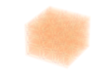
(a) $\mathcal{X}$

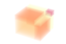
(b) Clustered $\mathcal{X}$

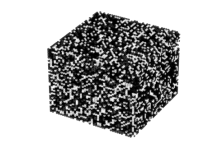
(c) $\mathcal{Y}$

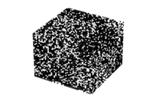
(d) Clustered $\mathcal{Y}$

Figure 1: In this example, the data tensor $\mathcal{Y}$ is a $40\times 40\times 40$-binary tensor and the underlying signal $\mathcal{X}$ has a symmetric core tensor $\mathcal{S}$ and the cluster structures are the same in every mode ($z_{1}=z_{2}=z_{3}$). Black dots represent value $1$, and zeros are not drawn.

Definition 2.2.

Given a labeling function $z\colon[n]\rightarrow[r]$ and an estimate $\hat{z}\colon[n]\rightarrow[r]$, the misclassification rate is defined as

$$\begin{split}\ell(z,\hat{z})&=\min_{\textup{permutation }\pi:[r]\rightarrow[r]}\frac{1}{n}\sum_{i=1}^{n}\mathbb{I}\{\pi(\hat{z}(i))\neq z(i)\}.\end{split}$$

An estimator $Y\mapsto\hat{z}(Y)$ is said to be weakly consistent if $\ell(z_{\nu},\hat{z}(Y_{\nu}))\rightarrow 0$ in probability as $\nu\rightarrow\infty$. An estimator $Y\mapsto\hat{z}(Y)$ is said to be strongly consistent if $\ell(z_{\nu},\hat{z}(Y_{\nu}))=0$ with high probability as $\nu\rightarrow\infty$.

From now on, we usually omit the index $\nu$ used in Definition 2.2. That is, instead of writing $x_{\nu}\gg y_{\nu}$ we may write $x\gg y$. Weak consistency is indicated by $\mathbb{P}(\ell(z,\hat{z})\geq\varepsilon)\rightarrow 0$ for all $\varepsilon>0$, and strong consistency is indicated by $\mathbb{P}(\ell(z,\hat{z})=0)\rightarrow 1$.

To control the amount of noise, the separation of clusters, and the amount of data per cluster, we will often assume the following.

Assumption 2.1 (MGF bound).

An integrable random variable $X$ is said to satisfy the MGF bound with variance proxy $\sigma^{2}\geq 0$ if

$$\mathbb{E}e^{\lambda(X-\mathbb{E}X)}\leq e^{\sigma^{2}(e^{\lvert\lambda\rvert}-1-\lvert\lambda\rvert)}\qquad\text{for all }\lambda\in\mathbb{R}.$$ (2.1)

Assumption 2.2 (Separation).

The clusters of $\operatorname{TBM}(\rho,\mathcal{S},z_{1},\dots,z_{d})$ are said to be separated along mode $k$, if there exists a constant $\delta_{k}>0$ (not depending on $\nu$) such that $\min_{l\neq l^{\prime}}\frac{\lVert(\operatorname{\textup{mat}}_{k}\mathcal{S})_{l:}-(\operatorname{\textup{mat}}_{k}\mathcal{S})_{l^{\prime}:}\rVert^{2}}{r_{1}\cdots r_{d}/r_{k}}\geq\delta_{k}^{2}$. The number $\delta_{k}$ is called a separation of mode $k$.

Assumption 2.3 (Balanced clusters).

A TBM with membership vectors $z_{k}$ is said to have balanced clusters if $\lvert z_{k}^{-1}\{l_{k}\}\rvert\asymp n_{k}/r_{k}$ for all $l_{k}$ and $k$. Then a constant $\alpha\in(0,1)$ (not depending on $\nu$) satisfying $\lvert z_{k}^{-1}\{l_{k}\}\rvert\geq\alpha n_{k}/r_{k}$ for all $l_{k}$ and $k$ is called a cluster balance coefficient.

Assumption 2.1 is stronger than the subexponential assumption but weaker than the subgaussian assumption. For example, Poisson distributions satisfy Assumption 2.1 but have heavier than Gaussian tails. For more details about what kind of random variables satisfy the MGF bound, see Lemma D.1. We refer to [39] for further details on subexponential and subgaussian distributions.

The term variance proxy is motivated by the fact that $\textup{Var}(X)\leq\sigma^{2}$ for every random variable $X$ satisfying Assumption 2.1. This follows from writing inequality (2.1) with Taylor series $1+\frac{\lambda^{2}\textup{Var}(X)}{2}+\mathcal{O}(\lambda^{3})\leq e^{\sigma^{2}\lambda^{2}/2+\mathcal{O}(\lambda^{3})}=1+\frac{\sigma^{2}\lambda^{2}}{2}+\mathcal{O}(\lambda^{3})$.

Example 2.1 (Bernoulli TBM).

Consider a TBM with Bernoulli distributed data entries $\mathcal{Y}_{i_{1}\dots i_{d}}\overset{d}{=}\operatorname{\textup{Ber}}(\mathcal{X}_{i_{1}\dots i_{d}})$ and a core tensor $\rho\mathcal{S}$, where $\rho\in[0,1]$ is a scalar controlling sparsity and $\mathcal{S}\in[0,1]^{r_{1}\times\dots\times r_{d}}$. Then the data entries have variances $\textup{Var}(\mathcal{Y}_{i_{1}\dots i_{d}})=\rho\mathcal{S}_{z_{1}(i_{1})\dots z_{d}(i_{d})}(1-\rho\mathcal{S}_{z_{1}(i_{1})\dots z_{d}(i_{d})})\leq\rho$ and the noise satisfies Assumption 2.1 with variance proxy $\rho$ (Lemma D.1:(ii)).

Example 2.2 (Poisson TBM).

Consider a TBM with Poisson distributed data entries $\mathcal{Y}_{i_{1}\dots i_{d}}\overset{d}{=}\operatorname{\textup{Poi}}(\mathcal{X}_{i_{1}\dots i_{d}})$ and a core tensor $\rho\mathcal{S}$, where $\rho\in[0,1]$ is a scalar controlling sparsity and $\mathcal{S}\in[0,1]^{r_{1}\times\dots\times r_{d}}$. Then the data entries have variances $\textup{Var}(\mathcal{Y}_{i_{1}\dots i_{d}})=\rho\mathcal{S}_{z_{1}(i_{1})\dots z_{d}(i_{d})}\leq\rho$ and the noise satisfies Assumption 2.1 with variance proxy $\rho$ (Lemma D.1:(vi)).

3 Main results

3.1 Algorithm

Algorithm 1 represents a spectral clustering algorithm for recovering a latent cluster structure along mode $k$. To estimate the cluster membership vectors of all modes, it may be run $d$ times, once for each mode.

input: Data tensor $\mathcal{Y}\in\mathbb{R}^{n_{1}\times\dots\times n_{d}}$, mode $k$, number of clusters $r_{k}$, trimming threshold $C_{\rm trim}\rho^{2}$, relaxation constant $Q>1$

output: Cluster membership vector $\hat{z}_{k}\colon[n_{k}]\rightarrow[r_{k}]$

Set $A$ to be the Gram matrix $(\operatorname{\textup{mat}}_{k}\mathcal{Y})(\operatorname{\textup{mat}}_{k}\mathcal{Y})^{T}$ with zeroed diagonal

Set $A_{ij}\leftarrow 0$ if $\sum_{j^{\prime},k:j^{\prime}\neq i}\lvert(\operatorname{\textup{mat}}_{k}\mathcal{Y})_{ik}(\operatorname{\textup{mat}}_{k}\mathcal{Y})_{j^{\prime}k}\rvert\geq C_{\rm trim}\rho^{2}n_{1}\cdots n_{d}$ or $\sum_{i^{\prime},k:i^{\prime}\neq j}\lvert(\operatorname{\textup{mat}}_{k}\mathcal{Y})_{i^{\prime}k}(\operatorname{\textup{mat}}_{k}\mathcal{Y})_{jk}\rvert\geq C_{\rm trim}\rho^{2}n_{1}\cdots n_{d}$

Compute the best rank-$r_{k}$ approximation $A=\hat{U}\hat{\Lambda}\hat{U}^{T}+\hat{U}_{\perp}\hat{\Lambda}_{\perp}\hat{U}_{\perp}^{T}\approx\hat{U}\hat{\Lambda}\hat{U}^{T}$, where $\hat{\Lambda}$ contains the $r_{k}$ largest eigenvalues in absolute value

Cluster the rows of $\hat{U}\hat{\Lambda}$ into $r_{k}$ clusters by finding a labeling function $\hat{z}_{k}$ and centroids $\hat{\theta}_{1},\dots,\hat{\theta}_{r_{k}}\in\mathbb{R}^{r_{k}}$ satisfying

$$\sum_{j}\lVert(\hat{U}\hat{\Lambda})_{j:}-\hat{\theta}_{\hat{z}_{j}}\rVert^{2}\leq Q\min_{\breve{z},\breve{\theta}}\sum_{j}\lVert(\hat{U}\hat{\Lambda})_{j:}-\breve{\theta}_{\breve{z}_{j}}\rVert^{2}$$

for example with $k$-means++ [2]

Algorithm 1 Hollow spectral clustering

To motivate Algorithm 1, consider a sample $\mathcal{Y}$ from $\operatorname{TBM}(\rho,\mathcal{S},z_{1},\dots,z_{d})$ (Definition 2.1). Define membership matrices $Z^{(k)}\in\{0,1\}^{n_{k}\times r_{k}}$ by $Z_{i_{k}j_{k}}^{(k)}=\mathbb{I}(z_{k}(i_{k})=j_{k})$ for each mode $k=1,\dots,d$. That is, $Z_{i_{k}j_{k}}^{(k)}$ indicates whether or not the cluster of the index $i_{k}$ along the mode $k$ is $j_{k}$. Then the signal tensor admits a Tucker decomposition

$$\mathcal{X}=\rho\mathcal{S}\times_{1}Z^{(1)}\times_{2}\dots\times_{d}Z^{(d)}.$$

From linear algebraic perspective, clustering amounts to inferring a low-rank Tucker decomposition from a perturbed data tensor. This motivates to estimate $\mathcal{X}$ by approximating $\mathcal{Y}$ with a low-rank Tucker decomposition, i.e., to minimize the distance

$$\lVert\mathcal{Y}-\breve{\mathcal{S}}\times_{1}\breve{U}^{(1)}\times_{2}\dots\times_{d}\breve{U}^{(d)}\rVert_{\rm F},$$ (3.1)

where the matrices $\breve{U}^{(k)}\in\mathbb{R}^{n_{k}\times r_{k}}$ are imposed to have orthonormal columns and $\breve{\mathcal{S}}\in\mathbb{R}^{r_{1}\times\dots\times r_{d}}$ is a tensor. Unfortunately, minimizing (3.1) is known to be NP-hard in general, already when the core dimensions are ones [22]. Nonetheless, fast algorithms have been developed to approximately minimize (3.1). These include higher-order singular value decomposition (HOSVD) [13], higher-order orthogonal iteration (HOOI) [14] and simple variations of these such as sequentially truncated HOSVD [38]. These are based on observing that the matricization $\operatorname{\textup{mat}}_{k}\mathcal{Y}$ is a noisy version of its expectation

$$\operatorname{\textup{mat}}_{k}\mathcal{X}\ =\ Z^{(k)}\operatorname{\textup{mat}}_{k}\left(\rho\mathcal{S}\times_{1}Z^{(1)}\times_{2}\dots\times_{k-1}Z^{(k-1)}\times_{k+1}Z^{(k+1)}\times_{k+2}\dots\times_{d}Z^{(d)}\right)$$

that has rank at most $r_{k}$. This motivates to estimate $\operatorname{\textup{mat}}_{k}\mathcal{X}$ with a rank-$r_{k}$ approximation of $\operatorname{\textup{mat}}_{k}\mathcal{Y}$, or alternatively, estimate $(\operatorname{\textup{mat}}_{k}\mathcal{X})(\operatorname{\textup{mat}}_{k}\mathcal{X})^{T}$ with a rank-$r_{k}$ approximation of $(\operatorname{\textup{mat}}_{k}\mathcal{Y})(\operatorname{\textup{mat}}_{k}\mathcal{Y})^{T}$. HOSVD repeats this rank approximation over each mode and HOOI iterates this type of computation multiple times. Algorithm 1, in turn, essentially does this rank approximation only once before the final clustering step. Although simple, this step is crucial for HOSVD as it provides the very first initialization.

After dimension reduction, Algorithm 1 clusters the low-dimensional vectors by solving $k$-means minimization task quasi-optimally. Exact minimization is known to be NP-hard in general [15], but quasi-optimal solutions can be found with fast implementations such as $k$-means++ with quasi-optimality constant $\mathcal{O}(\log r)$, where $r$ is the number of clusters [2]. Since $k$-means++ is a randomized algorithm, it is guaranteed to be quasi-optimal only in expectation rather than always.

Two key differences distinguish Algorithm 1 from standard spectral clustering. First, the diagonal entries of the Gram matrix $(\operatorname{\textup{mat}}_{k}\mathcal{Y})(\operatorname{\textup{mat}}_{k}\mathcal{Y})^{T}$ are zeroed giving a hollow Gram matrix. This modification has been considered already in [29]. Second, the obtained hollow Gram matrix is trimmed by removing carefully selected rows and columns. In the case of nonnegative data, those with too large $L_{1}$-norms are selected.

3.2 Consistency

The following theorem presents the main result of the paper. It confirms the weak consistency of Algorithm 1 for data sampled from a sparse integer-valued TBM (Definition 2.1).

Theorem 3.1 (Weak consistency).

Let $\mathcal{Y}\in\mathbb{Z}^{n_{1}\times\dots\times n_{d}}$ be a sample from $\operatorname{TBM}(\rho,\mathcal{S},z_{1},\dots,z_{d})$ with fixed $d$. Assume that the entries of the noise tensor $\mathcal{E}$ satisfy the MGF bound with variance proxy $\rho$ (Assumption 2.1) and $\mathbb{E}\lvert\mathcal{E}_{i_{1}\dots i_{d}}\rvert\leq\rho$. Assume also separated clusters along mode $k$ with separation $\delta>0$ (Assumption 2.2) and balanced clusters with cluster balance coefficient $\alpha$ (Assumption 2.3). Consider parameter regime

$$\frac{r_{k}^{3/2}}{\sqrt{n_{1}\cdots n_{d}}}\vee\frac{n_{k}\log n_{k}}{n_{1}\cdots n_{d}}\ll\rho\ll n_{k}^{-1}(n_{1}\cdots n_{d}/n_{k})^{-\varepsilon}$$ (3.2)

for some constant $\varepsilon>0$ and $r_{k}\ll n_{k}^{2/3}$. Then there exists a constant $C$ such that if $C_{\rm trim}\geq C\vee\varepsilon^{-1}$, then the estimated cluster membership vector $\hat{z}_{k}$ given by Algorithm 1 on mode $k$ is weakly consistent. Furthermore, the probability bound

$$\begin{split}&\mathbb{P}\left(\ell(z_{k},\hat{z}_{k})\geq s+CQ\left(\frac{r_{k}}{\alpha^{d-\frac{1}{2}}\delta^{2}}\left(\frac{1\vee\varepsilon^{-3}+C_{\rm trim}}{\sqrt{n_{1}\cdots n_{d}}\rho}+\frac{1}{n_{k}}\right)\right)^{2}\right)\\ &\leq\frac{1}{s}\left(\sqrt{C_{\rm trim}}e^{-n_{1}\cdots n_{d}\rho^{2}}+3n_{k}^{-1}\right)+Cn_{k}^{-1}e^{-1\vee\varepsilon^{-1}}\end{split}$$

holds eventually, when $s$ is chosen to satisfy $e^{-n_{1}\cdots n_{d}\rho^{2}}+n_{k}^{-1}\ll s\ll r_{k}^{-1}$.

Under extra assumptions $n_{1}=\dots=n_{d}=n$ and $r_{k}\asymp 1$, Condition (3.2) is equivalent to $d\geq 3$ and $n^{-d/2}\ll\rho\ll n^{-1-\varepsilon(d-1)}$.

3.3 Aggregation

High-order data is commonly analyzed by aggregating the data tensor into a lower-order data tensor. Theorem 3.2 shows that an aggregated TBM is also a TBM and the variance proxy of the noise entries scales accordingly. As a consequence, Corollary 3.3 shows that aggregating is beneficial for sparse data as long as the signal tensor remains well separated.

Theorem 3.2 (Aggregation).

Let $\mathcal{Y}\in\mathbb{Z}^{n_{1}\times\dots\times n_{d}}$ be a sample from $\operatorname{TBM}(\rho,\mathcal{S},z_{1},\dots,z_{d})$. Assume that the entries of the noise tensor $\mathcal{E}$ satisfy the MGF bound with variance proxy $\rho$ (Assumption 2.1) and $\mathbb{E}\lvert\mathcal{E}_{i_{1}\dots i_{d}}\rvert\leq\rho$. Then an aggregate data tensor $\mathcal{Y}^{\prime}\in\mathbb{Z}^{n_{1}\times\dots\times n_{d^{\prime}}}$ with entries $\mathcal{Y}_{i_{1}\dots i_{d^{\prime}}}^{\prime}=\sum_{i_{d^{\prime}+1},\dots,i_{d}}\mathcal{Y}_{i_{1}\dots i_{d}}$ is a sample from $\operatorname{TBM}(\rho^{\prime},\mathcal{S}^{\prime},z_{1},\dots,z_{d^{\prime}})$ with density $\rho^{\prime}=n_{d^{\prime}+1}\cdots n_{d}\rho$ and normalized core tensor $\mathcal{S}_{j_{1}\dots j_{d^{\prime}}}^{\prime}=\frac{1}{n_{d^{\prime}+1}\cdots n_{d}}\sum_{i_{d^{\prime}+1},\dots,i_{d}}\mathcal{S}_{j_{1}\dots j_{d^{\prime}}z_{d^{\prime}+1}(i_{d^{\prime}+1})\dots z_{d}(i_{d})}$. Furthermore, the entries of the noise tensor satisfy the MGF bound with variance proxy $\rho^{\prime}$ and $\mathbb{E}\lvert\mathcal{E}_{i_{1}\dots i_{d^{\prime}}}^{\prime}\rvert\leq\rho^{\prime}$.

Proof.

The MGF bound is a direct consequence of Lemma D.1:(iii). By the triangle inequality, $\mathbb{E}\lvert\mathcal{E}_{i_{1}\dots i_{d^{\prime}}}^{\prime}\rvert=\mathbb{E}\lvert\sum_{i_{d^{\prime}+1},\dots,i_{d}}\mathcal{E}_{i_{1}\dots i_{d}}\rvert\leq n_{d^{\prime}+1}\cdots n_{d}\rho$. ∎

Corollary 3.3 (Weak consistency in Aggregated TBM).

Let $\mathcal{Y}\in\mathbb{Z}^{n_{1}\times\dots\times n_{d}}$ be a sample from $\operatorname{TBM}(\rho,\mathcal{S},z_{1},\dots,z_{d})$ fixed $d$. Assume that the entries of the noise tensor $\mathcal{E}$ satisfy the MGF bound with variance proxy $\rho$ (Assumption 2.1) and $\mathbb{E}\lvert\mathcal{E}_{i_{1}\dots i_{d}}\rvert\leq\rho$. Let $\mathcal{Y}^{\prime}\in\mathbb{Z}^{n_{1}\times\dots\times n_{d^{\prime}}}$ be an aggregated data tensor as in Theorem 3.2 and assume that it has separated clusters along mode $k$ (Assumption 2.2) and balanced clusters (Assumption 2.3). Consider parameter regime

$$\frac{r_{k}^{3/2}}{\sqrt{n_{1}\cdots n_{d^{\prime}}}n_{d^{\prime}+1}\cdots n_{d}}\vee\frac{n_{k}\log n_{k}}{n_{1}\cdots n_{d}}\ll\rho\ll\frac{1}{n_{k}n_{d^{\prime}+1}\cdots n_{d}(n_{1}\dots n_{d^{\prime}}/n_{k})^{\varepsilon}}$$ (3.3)

for some constant $\varepsilon>0$ and $r_{k}\ll n_{k}^{2/3}$. Then there exists a constant $C$ such that if $C_{\rm trim}\geq C\vee\varepsilon^{-1}$, then Algorithm 1 applied to mode $k$ of $\mathcal{Y}^{\prime}$ is weakly consistent.

Proof.

The claim follows from Theorem 3.1 which is applicable by Theorem 3.2. ∎

Example 3.1.

Under extra assumptions $n_{1}=\dots=n_{d}=n$ and $r_{k}\asymp 1$, condition (3.3) is equivalent to $n^{-(d-d^{\prime}/2)}\ll\rho\ll n^{-(1+d-d^{\prime})-\varepsilon(d^{\prime}-1)}$, where the lower bound is orders of magnitude smaller than $n^{-d/2}$ for the nonaggregated model in Theorem 3.1. That is, aggregating allows to handle much sparser data as it improves the density threshold by a factor $n^{-1/2}$ per aggregated mode. However, Assumption 2.2 for an aggregated TBM is stronger as it considers separation in $\mathcal{S}^{\prime}$.

4 Numerical experiments

This section presents numerical experiments to demonstrate the performance of Algorithm 1 in various sparsity regimes.

4.1 Setup

We focus on third-order tensors. The signal tensor is chosen to be symmetric so that the mode chosen for matricization does not matter. That is, the normalized core tensor $\mathcal{S}\in\mathbb{R}^{2\times 2\times 2}$ is symmetric, the observation tensor is a cube $\mathcal{Y}\in\mathbb{Z}^{n\times n\times n}$, and every mode has the same membership vector $z\in\{1,2\}^{n}$. The number of clusters is fixed to $r=2$ for visualization purposes, as the low-dimensional projections are then $2$-dimensional. The two clusters are equal sized and have constant degrees, i.e.,

$$\mathbb{E}\sum_{i_{2}i_{3}}\mathcal{Y}_{i_{1}i_{2}i_{3}}=\sum_{i_{2}i_{3}}\rho\mathcal{S}_{z(i_{1})z(i_{2})z(i_{3})}=\frac{n^{2}\rho}{4}\sum_{s,t}\mathcal{S}_{z(i_{1})st}$$

is independent of $z(i_{1})$. This implies that aggregating the data into an order-$1$ tensor loses information. Similar to hypergraphs, the data tensor is assumed to be binary $\mathcal{Y}\in\{0,1\}^{n\times n\times n}$ so that all entries are independent Bernoulli random variables (see Example 2.1). In a single experiment, the normalized core tensor $\mathcal{S}$ is fixed, and the unnormalized core tensor is $\rho\mathcal{S}$, where $\rho$ is allowed to vary. Now, the model can be written as

$$\mathcal{Y}_{i_{1}i_{2}i_{3}}\overset{d}{=}\operatorname{Ber}(\rho\mathcal{S}_{z(i_{1})z(i_{2})z(i_{3})}).$$

We investigate two instances of the normalized core tensor $\mathcal{S}$, one with informative aggregation and one with noninformative. Recall that aggregating one mode yields $\operatorname{TBM}(\rho^{\prime},\mathcal{S}^{\prime},z,z)$ with a density parameter $\rho^{\prime}=n\rho$ and a normalized core tensor $\mathcal{S}_{l_{1}l_{2}}^{\prime}=\frac{1}{n}\sum_{i_{3}}\mathcal{S}_{l_{1}l_{2}z(i_{3})}=\frac{1}{2}(\mathcal{S}_{l_{1}l_{2}1}+\mathcal{S}_{l_{1}l_{2}2})$ (Theorem 3.2). By writing $\mathcal{S}=\begin{bmatrix}\mathcal{S}_{::1}&\mathcal{S}_{::2}\end{bmatrix}$, the two considered normalized core tensors and their aggregated versions are

$$\mathcal{S}_{\rm informative}=\begin{bmatrix}1&0&0&0\\ 0&0&0&1\end{bmatrix}, \mathcal{S}_{\rm noninformative}=\begin{bmatrix}1&0&0&1\\ 0&1&1&0\end{bmatrix},$$

$$\mathcal{S}_{\rm informative}=\begin{bmatrix}1/2&0\\ 0&1/2\end{bmatrix}, \mathcal{S}_{\rm noninformative}^{\prime}=\begin{bmatrix}1/2&1/2\\ 1/2&1/2\end{bmatrix}.$$

These are visualized in Figure 2.

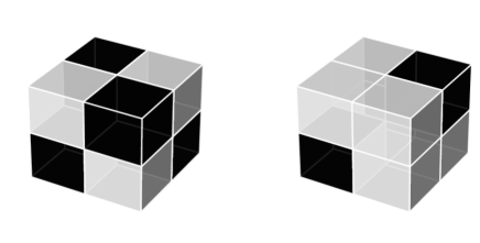
Figure 2: Symmetric core tensors $\mathcal{S}$ used in simulation experiments. Threeway $2\times 2\times 2$ arrays are represented as cubes, where black color corresponds to value $1$ and white color corresponds to value $0$. The cube on the left depicts the core tensor with a noninformative aggregate matrix and the cube on the right with an informative aggregate matrix.

Different algorithms are tested for various pairs $(n,\rho)$ and the proportion of correctly clustered nodes is recorded. Since the phase transition is expected to be at $\rho=Cn^{-\gamma}$ for some constant $C$ and exponent $\gamma$ depending on the algorithm, in logarithmic coordinates, this corresponds to a linear equation $\log\rho=C-\gamma\log n$ with slope $-\gamma$. Hence, the algorithms are tested on a grid of pairs $(n,\rho)$, where values of $n$ and $\rho$ are spaced logarithmically. Then, a line is fitted in logarithmic coordinates to estimate the phase transition and this is compared to the theoretical line. In detail, the phase transition line is estimated via logistic regression by first predicting whether the proportion of correctly clustered nodes is sufficiently high (e.g. $0.9$) given $(\log n,\log\rho)$ and then the learned decision boundary is used as the estimate for the phase transition line. Although this might not be an optimal estimator of the phase transition line, visually this produces meaningful results. A line with theoretical slope $-\gamma$ is drawn to visualize how well the simulated phase transition line fits to the theory.

The following four algorithms are compared.

1. Hollow SVD (Algorithm 1 with a known parameter $\rho$ and a trimming constant $C_{\rm trim}=3$). By Theorem 3.1, we expect the phase transition line to have $\gamma=1.5$.

2. SVD. A simple spectral clustering which is otherwise the same as Algorithm 1 but without trimming and diagonal masking. We expect the phase transition line to have $\gamma\approx 1.33$. Namely, the diagonal entries of the data Gram matrix $(\operatorname{\textup{mat}}_{1}\mathcal{Y})(\operatorname{\textup{mat}}_{1}\mathcal{Y})^{T}$ have standard deviations

   $$\begin{split}\operatorname{\textup{SD}}(((\operatorname{\textup{mat}}_{1}\mathcal{Y})(\operatorname{\textup{mat}}_{1}\mathcal{Y})^{T})_{i_{1}i_{1}})&=\operatorname{\textup{SD}}\left(\sum_{i_{2},i_{3}}\mathcal{Y}_{i_{1}i_{2}i_{3}}^{2}\right)=\sqrt{\sum_{i_{2},i_{3}}\textup{Var}(\mathcal{Y}_{i_{1}i_{2}i_{3}}^{2})}\overset{\mathcal{Y}_{i_{1}i_{2}i_{3}}^{2}=\mathcal{Y}_{i_{1}i_{2}i_{3}}}{\asymp}n\sqrt{\rho},\end{split}$$

   which dominate the operator norm of the signal Gram matrix

   $$\begin{split}\lVert(\operatorname{\textup{mat}}_{1}\mathcal{X})(\operatorname{\textup{mat}}_{1}\mathcal{X})^{T}\rVert_{\rm op}&\overset{(*)}{\asymp}\lVert(\operatorname{\textup{mat}}_{1}\mathcal{X})(\operatorname{\textup{mat}}_{1}\mathcal{X})^{T}\rVert_{\rm F}=\sqrt{\sum_{i_{1},i_{1}^{\prime}}\left(\sum_{i_{2},i_{3}}\mathcal{X}_{i_{1}i_{2}i_{3}}\mathcal{X}_{i_{1}^{\prime}i_{2}i_{3}}\right)^{2}}\asymp n^{3}\rho^{2},\end{split}$$

   when $\rho\ll n^{-4/3}$. Here $(*)$ follows from the fact that the operator norm and Frobenius norm of low-rank matrices are comparable, see for example Corollary 2.4.3 and Problem P2.4.7 in [20].

3. HSC. A simplification of the high-order spectral clustering (HSC) proposed in [21]. First, HSC calculates a low-rank approximation of the data tensor with HOSVD [13] and essentially one iteration of HOOI [14]. In our simplification, HOSVD matricizes the data tensor and calculates its SVD only once since as the underlying signal tensor is symmetric. This will slightly speed up the computations. Then the algorithm clusters the first mode of the low-rank tensor with $k$-means++. Since HSC is initialized with a simple rank-approximation (via eigenvalue decomposition of $(\operatorname{\textup{mat}}_{1}\mathcal{Y})(\operatorname{\textup{mat}}_{1}\mathcal{Y})^{T}$), it is expected not to improve $\gamma$. That is, we expect $\gamma\approx 1.33$.

4. Aggregate SVD. Spectral clustering from an aggregate matrix, which is a simplified version of an algorithm proposed in [43]. In this experiment, the algorithm computes the aggregate matrix $A_{ij}=\sum_{k}\mathcal{Y}_{ijk}$, removes rows and columns with too large $L_{1}$ norms (trimming threshold $C_{\rm trim}n^{2}\rho$ with $C_{\rm trim}=3$), calculates the best rank-$2$ approximation, and then clusters the rows with $k$-means++ [2]. In the original paper, the data tensor is symmetric and hence there are small differences in calculating $A$. Furthermore, the actual clustering step is not implemented with $k$-means++ and there is a final refinement step, but morally these algorithms are the same. We expect the phase transition line to have $\gamma=2$ if the aggregate matrix is informative.

4.2 Results

Figure 3 shows a comparison of the four algorithms when the aggregate matrix is not informative. As expected, spectral clustering on the aggregate matrix gives poor results, whereas the other three algorithms show a clear phase transition. The observed phase transition is in line with the expected phase transition. The refining steps in HSC do not improve the exponent $\gamma$ compared to the plain SVD, but they do improve the clustering performance significantly. Although the estimated $\gamma$-exponents differ from the expected exponents slightly, they would be hard to distinguish from the expected exponents visually.

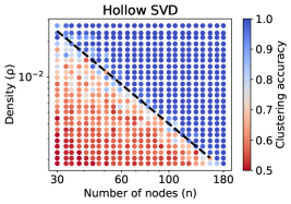
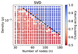
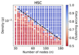
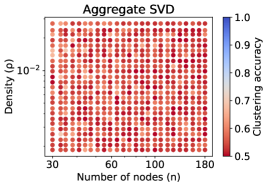
Figure 3: Comparison of the four algorithms when the aggregate matrix is not informative. The number of nodes varies logarithmically between $30$ and $180$, and the sparsity parameter varies logarithmically between $0.00185$ and $0.02722$. The dashed black line is the fitted phase transition line with theoretical slope ($\gamma_{\rm Hollow\ SVD}=1.5$, $\gamma_{\rm SVD}=1.33$, $\gamma_{\rm HSC}=1.33$). The estimated slopes given by logistic regression are $\hat{\gamma}_{\rm Hollow\ SVD}=1.43$, $\hat{\gamma}_{\rm SVD}=1.29$ and $\hat{\gamma}_{\rm HSC}=1.26$.

Figure 4 shows a comparison of the four algorithms when the aggregate matrix is informative. As expected, spectral clustering on the aggregate matrix gives the best results. The observed phase transition is in line with the expected phase transition. Although the estimated $\gamma$-exponents differ from the expected exponents slightly, they would be hard to distinguish from the expected exponents visually.

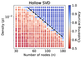
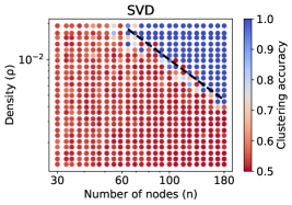
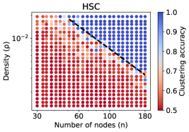
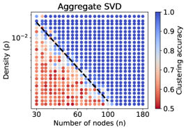
Figure 4: Comparison of the four algorithms when the aggregate matrix is informative. The number of nodes varies logarithmically between $30$ and $180$, and the sparsity parameter varies logarithmically between $0.00131$ and $0.01925$. The dashed black line is the fitted phase transition line with theoretical slope ($\gamma_{\rm Hollow\ SVD}=1.5$, $\gamma_{\rm SVD}\approx 1.33$, $\gamma_{\rm HSC}\approx 1.33$, $\gamma_{\rm Aggregate\ SVD}=2$). The estimated slopes given by logistic regression are $\hat{\gamma}_{\rm Hollow\ SVD}=1.43$, $\hat{\gamma}_{\rm SVD}=1.31$, $\hat{\gamma}_{\rm HSC}=1.24$ and $\hat{\gamma}_{\rm Aggregate\ SVD}=2.00$.

4.3 HSC initialization

Previous simulations demonstrate that HSC does not improve the exponent $\gamma$ of its initialization algorithm. This subsection studies visually, how HSC depends on its initialization algorithm, and how it is possible that for some pairs of $n$ and $\rho$, the initialization algorithm does not cluster the nodes successfully while HSC does.

Similar to the experiment with a noninformative aggregate matrix, we consider a symmetric normalized core tensor

$$\mathcal{S}=\begin{bmatrix}1&0.5&0.5&1\\ 0.5&1&1&0.5\end{bmatrix}.$$

The only difference is that the entries with value $0$ have been changed to the value $0.5$. If the entries were zero, then any two row vectors of $\operatorname{\textup{mat}}_{k}\mathcal{Y}$ from different clusters would be orthogonal. This, in turn, usually makes the projected row vectors to lie on two orthogonal lines representing different clusters, and the projected row vectors would overlap with each other in the visualization. Furthermore, when testing HSC, the initialization algorithm is changed from simple SVD to the proposed hollow SVD, because without any trimming step near the phase transition, there would be “outliers” with significantly larger norms, which would force the visualizations to focus on the outliers.

Figure 5 shows the obtained projections from the initialization algorithm (hollow SVD) and HSC for four different sparsity parameters. As the sparsity parameter decreases, the clusters merge in the projections. It may occur that the initialization provides somewhat meaningful projections, but the $k$-means algorithm cannot detect the clusters. However, such initialization might be informative enough for HSC to improve the projection and cluster the vectors. However, as expected, once the initialization is dominated by noise, HSC cannot cluster the vectors.

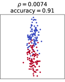
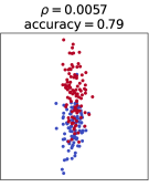
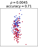
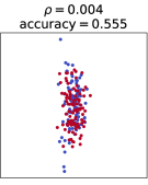
(a) Hollow SVD

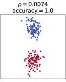
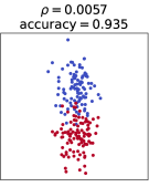
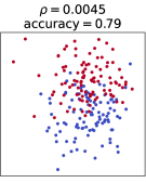
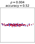
(b) Hollow HSC

Figure 5: Projected observations with (a) hollow SVD and (b) HSC initialized with hollow SVD. The number of nodes is fixed to $n=200$ and the sparsity parameter $\rho$ is varied around the phase transition. Sparsity decreases from left to right. Accuracy ($1-\ell$) of $k$-means clustering is also recorded.

5 Discussion

5.1 Clustering

This section discusses related theoretical research on multiway clustering with emphasis on recent developments on hypergraphs, and temporal and multilayer networks.

Zhang and Tan [43] considered clustering of a $d$-uniform hypergraph on $n$ nodes, which is comparable to a TBM of order $d$ with Bernoulli distributed entries. The nodes have a fixed prior distribution over clusters and the signal is assumed to have a core tensor $\rho\mathcal{S}$ with fixed $\mathcal{S}$. They show that strong consistency is impossible, when $\rho\leq c\frac{\log n}{n^{d-1}}$ for sufficiently small constant $c$. Furthermore, they showed that a spectral clustering algorithm applied to an aggregate matrix $A_{i_{1}i_{2}}=\sum_{i_{3}\dots i_{d}}\mathcal{Y}_{i_{1}\dots i_{d}}$ achieves strong consistency for $\rho\geq C\frac{\log n}{n^{d-1}}$ for sufficiently large constant $C$, assuming that $\mathbb{E}A$ is informative (see [43] for further details on the constants $c,C$). The matrix $A$ can be considered as an adjacency matrix since for a symmetric tensor $\mathcal{Y}$ with $\mathcal{Y}_{i_{1}\dots i_{d}}=0$ whenever $i_{k}=i_{l}$ for some $k\neq l$ (undirected $d$-uniform hypergraph), $A$ is a symmetric matrix with upper-diagonal entries

$$\begin{split}A_{i_{1}i_{2}}&=\sum_{i_{3},\dots,i_{d}}\mathcal{Y}_{i_{1}\dots i_{d}}=(d-2)!\sum_{i_{3}<\dots<i_{d}}\mathcal{Y}_{i_{1}\dots i_{d}}=(d-2)!\sum_{\text{hyperedge }e}\mathbb{I}\{\{i_{1},i_{2}\}\subset e\},\qquad i_{1}<i_{2}.\end{split}$$

That is, up to a multiplicative constant (which for $d\leq 3$ is simply $1$), $A_{i_{1}i_{2}}$ counts the number of common hyperedges between nodes $i_{1}$ and $i_{2}$. Visually, this is equivalent to transforming a hypergraph to a (weighted) graph such that every hyperedge $\{i_{1},\dots,i_{d}\}$ contributes to an edge $\{j_{1},j_{2}\}\subset\{i_{1},\dots,i_{d}\}$, $j_{1}\neq j_{2}$. Stephan and Zhu [35] showed that a spectral clustering algorithm based on nonbacktracking walks on a hypergraph achieves weak reconstruction (i.e., is better than clustering every node to the largest cluster), if $\rho\gtrsim n^{1-d}$ and $\mathbb{E}A$ is informative. However, these results do not address the case when $\mathbb{E}A$ is not informative. Figure 1 visualizes an example of a tensor, for which the adjacency matrix would not be informative.

There has been research on multiway clustering with a noninformative adjacency matrix $A$. Lei, Chen and Lynch [28] analyzed an undirected multilayer network model, which can be formulated as a TBM with $\mathcal{Y}\in\{0,1\}^{m\times n\times n}$ with no cluster structure on the first mode (or $z_{1}(i)=i$, i.e., every index forms one cluster) and identical cluster structures on the second and third modes $z_{2}=z_{3}=z$, $r_{2}=r_{3}=r$. Each slice $\mathcal{Y}_{i::}$ corresponds to a symmetric adjacency matrix of an undirected network layer in a multilayer network. They consider a clustering algorithm solving a least-squares problem

$$(\hat{Z},\hat{\mathcal{S}})=\operatorname*{\textup{arg\,min}}_{\breve{Z},\ \breve{\mathcal{S}}}\lVert\mathcal{Y}-\mathcal{S}\times_{2}\breve{Z}\times_{3}\breve{Z}\rVert_{\rm F}^{2}$$

with a membership matrix $\breve{Z}\in\{0,1\}^{n\times r}$ and a core tensor $\breve{S}\in[0,1]^{m\times r\times r}$. They did not give an algorithm finding an exact or provably approximate solution, but they did provide an algorithm trying to solve the optimization problem. They showed that $\hat{Z}$ achieves weak consistency, when $\rho\gg\frac{\log^{3/2}n}{nm^{1/2}}$. Lei and Lin [29] analyzed a similar problem and proposed an algorithm similar to Algorithm 1. Specifically, their algorithm masks out the diagonal (which they call debiasing or bias adjusting) but it does not remove the nodes with too large $L_{1}$-norms. Their algorithm is guaranteed to be weakly consistent for $\rho\gg\frac{\log^{1/2}(n+m)}{nm^{1/2}}$. Ke, Shi and Xia [25] proved an analogous result for hypergraph degree-corrected block models. Su, Guo, Chang and Yang [36] extended these results and ideas to directed multilayer networks. The proof requires a matrix concentration inequality based on classical matrix Bernstein’s inequalities (see for example [37]). However, matrix Bernstein’s inequalities, which may be based on a deep theorem by Lieb depending on the proof, suffer from a logarithmic factor leading to the threshold $\frac{\log^{1/2}(n+m)}{nm^{1/2}}$ instead of $\frac{1}{nm^{1/2}}$.

Lei, Zhang and Zhu [31] studied computational and information theoretical limits of the multilayer network model corresponding to a TBM with $\mathcal{Y}\in\{0,1\}^{m\times n\times n}$ with no cluster structure on the first mode. They showed that weak consistency is impossible for $\rho\ll\frac{1}{nm}$ and the maximum likelihood estimator is weakly consistent for $\rho\gg\frac{1}{nm}$. Furthermore, based on a conjecture, they showed that a polynomial-time algorithm cannot be weakly consistent for $\rho\leq\frac{1}{2nm^{1/2}\log^{1.4}n}$. Kunisky [27] studied the impossibility of detecting a presence of a cluster structure in symmetric tensors with low coordinate degree functions (LCDF). LCDFs are arbitrary linear combinations of functions depending on at most $D$ entries of a vector, in our case the data tensor. Here the coordinate degree $D$ is argued to roughly correspond to algorithms requiring computation time $e^{\Theta(D)}$. Although the developed theory is more general, in the our special case Theorem 1.13 states that the detection task is impossible if $\rho\leq cn^{-\frac{d}{2}}D^{-\frac{d-2}{2}}$ for a sufficiently small constant $c$ and $D\leq cn$. Since polynomial-time algorithms correspond to $D\asymp\ln n$, the threshold corresponds roughly to $\rho\leq cn^{-\frac{d}{2}}\log^{-\frac{d-2}{2}}n$. Moreover, Kunisky showed that the detection task becomes easier when an aggregated tensor remains informative, each aggregated mode decreasing the density threshold by $n^{-\frac{1}{2}}$. This agrees with our Corollary 3.3.

Similar but slightly sharper computational gaps have been established in subgaussian noise. Han, Luo, Wang, and Zhang [21] analyzed multiway clustering on a TBM with subgaussian noise. Their algorithm is initialized with a slightly refined version of a HOSVD algorithm, which involves calculating eigenvalue decompositions of $(\operatorname{\textup{mat}}_{k}\mathcal{Y})(\operatorname{\textup{mat}}_{k}\mathcal{Y})^{T}$ without removing the diagonals or rows and columns with too large $L_{1}$-norms. They showed that HOSVD-based of initialization is weakly consistent for $\rho^{2}/\sigma^{2}\gg n^{-d/2}$, where $\sigma$ is the largest subgaussian norm of $\mathcal{E}_{i_{1}\dots i_{d}}$ (i.e., $\sigma^{2}$ is the largest variance proxy). When HOSVD-based initialization is given to an iterative higher-order Lloyd algorithm, they showed that the clustering is strongly consistent if $\rho^{2}/\sigma^{2}\geq Cn^{-d/2}$ for sufficiently large constant $C$. Furthermore, they show that strong consistency is not achievable for $\rho^{2}/\sigma^{2}\leq cn^{1-d}$ with a small enough constant $c$ while Wang and Zeng [41] show that maximum likelihood estimator is strongly consistent for $\rho^{2}/\sigma^{2}\geq Cn^{1-d}$ with a sufficiently large constant $C$. Notice that this threshold is similar to Theorem 3.1, namely both $\sigma^{2}$ and $\rho$ are an upper bounds of the variance of the data entries and setting $\sigma^{2}=\rho$ yields the same weak consistency condition $\rho\gg n^{-d/2}$. However, subgaussian analysis with Bernoulli distributed entries does not give $\sigma^{2}\asymp\rho$ but

$$\sigma^{2}=\frac{1-2\rho}{2\log\frac{1-\rho}{\rho}}\sim\frac{1}{2\log\frac{1}{\rho}}$$

as $\rho\rightarrow 0$ by Theorem 2.1 in [6]. For example, by setting $\rho=n^{-\gamma}$ with fixed $\gamma$ gives $\sigma^{2}\asymp\log^{-1}n$ which is substantially larger than $\rho=n^{-\gamma}$. Nonetheless, it seems that the analogous statistical-computational gap $\frac{\log n}{n^{d-1}}\lesssim\rho\ll\frac{1}{n^{d/2}}$ is present in clustering a binary TBM.

5.2 Random matrix norm bounds

Proving matrix concentration inequalities for a sparse Bernoulli matrix is more involved than for a subgaussian matrix. Kahn and Szemerédi [19] bound the second largest eigenvalue of an adjacency matrix of a random regular graph (random graphs with constant degree) and Feige and Ofek [18] repeat the same arguments for Erdős–Rényi graphs (symmetric adjacency matrix with lower diagonal having independent and identically distributed entries). Lei and Rinaldo [30] extend Feige’s and Ofek’s argument to bound the operator norm of a centered symmetric binary matrices with independent but possibly not identically distributed entries. With this they are able to show consistency of a spectral clustering algorithm under a stochastic block model, which is similar to a TBM with $d=2$. Chien, Lin, and Wang [9] extend this further to a centered adjacency matrix of a hypergraph stochastic block model (similar to binary TBM) to show strong consistency of a spectral clustering algorithm. Zhang and Tan [43] relax some parametric assumptions made in [9]. We also apply the proof techniques developed in [19] and [18].

In the context of clustering multilayer networks, Lei, Chen and Lynch [28] adapt Feige’s and Ofek’s argument to tensor setting. Lei and Lin [29] consider alternative approach by applying matrix concentration inequality based on classical matrix Bernstein’s inequalities (see for example [37]). However, matrix Bernstein’s inequalities, which may be based on a deep theorem by Lieb depending on the proof, suffer from a logarithmic factor making the matrix bounds slightly suboptimal.

In the case of subgaussian TBM, Han, Luo, Wang, and Zhang [21] approach by analyzing concentration of a singular subspace of a possibly wide random matrix (i.e., a vector subspace spanned by the first $r$ right or left singular vectors corresponding to the $r$ largest singular values of a random matrix). For this purpose, the classical Davis–Kahan–Wedin theorem is insufficient as it provides a common error bound for both left and right singular subspaces. Hence, they rely on more sophisticated perturbation bounds developed by Cai and Zhang [7] providing different bounds for left and right singular subspaces which is relevant for particularly tall and wide matrices. The probabilistic analysis is based on $\varepsilon$-nets and Hanson–Wright inequality (see for example Chapter 6 in [39]).

6 Proofs

This section presents the proof of the main theorem (Theorem 3.1) in three subsections. Section 6.1 analyzes spectral clustering with deterministic error bounds, Section 6.2 studies concentration of sparse matrices and Section 6.3 proves the main theorem. As the analysis of matrix concentration is quite involved, the detailed proofs of Section 6.2 are postponed to the appendix.

6.1 Deterministic analysis

The following theorem states that a low-rank approximation of a data matrix allows efficient clustering, when the noise level measured with operator norm is sufficiently small. The proof is similar to the proofs of Lemma 4 in [43], Theorem 3 in [21], Lemma 5.3 in [30], and Theorem 2.2 in [24]. However, [43], [21] and [24] included this step into consistency theorems involving statistical models not appropriate for our purposes and [30] is restricted to clustering from square matrices.

Theorem 6.1.

Let $X\in\mathbb{R}^{n\times m}$ be a matrix with $r$ distinct rows represented by $X_{i:}=S_{z(i):}$, where $S\in\mathbb{R}^{r\times m}$ and $z\in[r]^{n}$. Let $Y\in\mathbb{R}^{n\times m}$ be another matrix and $\hat{X}$ be its best rank-$r$ approximation. Let $\hat{z}$ be the output of a quasi-optimal $k$-means clustering algorithm applied to the rows of $\hat{X}$, i.e., find a labeling function $\hat{z}\colon[n]\rightarrow[r]$ and centroids $\hat{\theta}_{1},\dots,\hat{\theta}_{r}\in\mathbb{R}^{m}$ satisfying

$$\sum_{j}\lVert\hat{X}_{j:}-\hat{\theta}_{\hat{z}_{j}}\rVert^{2}\leq Q\min_{\breve{z},\breve{\theta}}\sum_{j}\lVert\hat{X}_{j:}-\breve{\theta}_{\breve{z}_{j}}\rVert^{2}$$

with some relaxation parameter $Q>1$. Assume that $\lvert z^{-1}\{k\}\rvert>128Q\frac{r\lVert Y-X\rVert_{\rm op}^{2}}{\Delta^{2}}$ for all $k$, where $\Delta=\min\{\lVert X_{i:}-X_{j:}\rVert\mid X_{i:}\neq X_{j:}\}$. Then the misclassification rate (recall Definition 2.2) has an upper bound

$$\ell(z,\hat{z})\leq 128Q\frac{r\lVert Y-X\rVert_{\rm op}^{2}}{n\Delta^{2}}.$$

Proof.

Define $E=Y-X$. Calculate a singular value decomposition $Y=\hat{U}\hat{\Sigma}\hat{V}^{T}+\hat{U}_{\perp}\hat{\Sigma}_{\perp}\hat{V}_{\perp}^{T}$ and define $\hat{X}=\hat{U}\hat{\Sigma}\hat{V}^{T}$, which is the best $r$-rank approximation of $Y$ (in statistical applications $\hat{X}$ is used to estimate $X$). Since the rank of $\hat{X}$ is at most $r$ and the rank of $X$ is at most $r$, the rank of their difference $\hat{X}-X$ is at most $2r$ (every vector $u$ of the image of $\hat{X}-X$ can be written as $u=u_{1}+u_{2}$, where $u_{1}\in\operatorname{im}\hat{X}$ is in an $r$-dimensional subspace and $u_{2}\in\operatorname{im}X$ is in another $r$-dimensional subspace). By Corollary 2.4.3 in [20], the Frobenius norm and the operator norm of the rank-$2r$ matrix $\hat{X}-X$ are comparable according $\lVert\hat{X}-X\rVert_{\rm F}^{2}\leq 2r\lVert\hat{X}-X\rVert_{\rm op}^{2}$. Now by the Eckart–Young–Mirsky theorem [17] and Weyl’s inequality [42], we have

$$\begin{split}\lVert\hat{X}-X\rVert_{\rm F}^{2}&\leq 2r\lVert\hat{X}-X\rVert_{\rm op}^{2}\leq 2r(\lVert\hat{X}-Y\rVert_{\rm op}+\lVert E\rVert_{\rm op})^{2}\overset{\rm EYM}{\leq}2r(\sigma_{r+1}(Y)+\lVert E\rVert_{\rm op})^{2}\\ &\overset{\rm Weyl}{\leq}2r(\sigma_{r+1}(X)+\lVert E\rVert_{\rm op}+\lVert E\rVert_{\rm op})^{2}\leq 8r\lVert E\rVert_{\rm op}^{2}.\\ \end{split}$$

This shows that the estimate $\hat{X}$ is close to $X$ in Frobenius norm. Denote the estimated clusters by $\hat{z}_{j}\in[r]$, $j=1,\dots,n$ and their centers by $\hat{\theta}_{k}\in\mathbb{R}^{m}$, $k=1,\dots,r$. By quasi-optimality, we have

$$\begin{split}\sum_{j}\lVert\hat{X}_{j:}-\hat{\theta}_{\hat{z}_{j}}\rVert^{2}&\leq Q\min_{\breve{z},\breve{\theta}}\sum_{j}\lVert\hat{X}_{j:}-\breve{\theta}_{\breve{z}_{j}}\rVert^{2}\leq Q\sum_{j}\lVert\hat{X}_{j:}-X_{j:}\rVert^{2}=Q\lVert\hat{X}-X\rVert_{\rm F}^{2}\leq 8Qr\lVert E\rVert^{2}.\end{split}$$

This shows that the row vectors of the estimate $\hat{X}$ are close to the estimated cluster means on average. Now we can estimate the distances between the true cluster means (rows of $S$) and the estimated cluster means ($\hat{\theta}_{\hat{z}_{j}}$):

$$\begin{split}\sum_{j}\lVert X_{j:}-\hat{\theta}_{\hat{z}_{j}}\rVert^{2}&\leq 2\sum_{j}\lVert X_{j:}-\hat{X}_{j:}\rVert^{2}+\lVert\hat{X}_{j:}-\hat{\theta}_{\hat{z}_{j}}\rVert^{2}\leq 32Qr\lVert E\rVert^{2}.\\ \end{split}$$

For any $t>0$, Markov’s inequality (with respect to the counting measure) gives

$$\begin{split}\lvert\{j\mid\lVert\hat{\theta}_{\hat{z}_{j}}-X_{j}\rVert^{2}\geq t^{2}\}\rvert&\leq\frac{\sum_{j}\lVert\hat{\theta}_{\hat{z}_{j}}-X_{j}\rVert^{2}}{t^{2}}\leq\frac{32Qr\lVert E\rVert^{2}}{t^{2}}.\end{split}$$

Consider the set $A=\{j\in[n]\mid\lVert\hat{\theta}_{\hat{z}_{j}}-X_{j}\rVert<t\}$. If $z_{i}\neq z_{j}$ for $i,j\in A$, then

$$\begin{split}\lVert\hat{\theta}_{\hat{z}_{i}}-S_{z_{j}}\rVert&\geq\lVert S_{z_{i}}-S_{z_{j}}\rVert-\lVert S_{z_{i}}-\hat{\theta}_{\hat{z}_{i}}\rVert>\Delta-t.\end{split}$$

If $z_{i}=z_{j}$ for some $i,j\in A$, then $\lVert\hat{\theta}_{\hat{z}_{i}}-S_{z_{j}}\rVert<t$. Consider $t$ satisfying $\Delta-t=t$, or equivalently, $t=\Delta/2$. Previous calculation shows, that for every $i,j\in A$, $z_{i}=z_{j}$ if and only if $\lVert\hat{\theta}_{\hat{z}_{i}}-S_{z_{j}}\rVert<\Delta/2$. This gives a well-defined mapping $\pi:\hat{z}(A)\rightarrow[r]$, $\pi(\hat{z}_{i})=z_{i}$ (if $\hat{z}_{i}=\hat{z}_{j}$, then $\lVert\hat{\theta}_{\hat{z}_{i}}-S_{z_{j}}\rVert<\Delta/2$ and hence $z_{i}=z_{j}$). However, $\pi$ is not bijective in general, when balanced cluster sizes are not assumed.

If $z|_{A}:A\rightarrow[r]$ is not a surjection, i.e., there exists $k\in[r]$ such that $z_{i}\neq k$ for every $i\in A$, then $z^{-1}\{k\}\subset A^{c}$, $\lvert z^{-1}\{k\}\rvert\leq\lvert A^{c}\rvert$. This is a contradiction if we assume that $\frac{32Qr\lVert E\rVert_{\rm op}^{2}}{t^{2}}<\lvert z^{-1}\{k\}\rvert$ for every $k$. Under this assumption, $z|_{A}$ is surjective and hence $\pi:\hat{z}(A)\rightarrow[r]$ is surjective (if $k\in[r]$, there exists $i\in A$ such that $k=z_{i}=\pi(\hat{z}_{i})$). The surjectivity of $\pi$ gives $\lvert\hat{z}(A)\rvert\geq\lvert[r]\rvert=r$ implying $\hat{z}(A)=[r]$ and making $\pi$ a bijection. The bound for the misclassification rate follows now from the estimate $\ell(z,\hat{z})\leq\lvert A^{c}\rvert/n$ ∎

As Theorem 6.1 shows, clustering from a low-rank approximation works well when the operator norm of the noise matrix is sufficiently small and the clusters are sufficiently separated in the signal. The following result (Lemma 6.2) addresses the latter issue by estimating the separation of clusters $\Delta$ in Theorem 6.1 under Assumptions 2.3 and 2.2. The former issue is addressed in Section 6.2.

Lemma 6.2.

Consider a TBM with a signal tensor $\mathcal{X}$. Assume separated clusters along mode $k$ with separation $\delta>0$ (Assumption 2.2) and balanced clusters with cluster balance coefficient $\alpha$ (Assumption 2.3). Then

$$\min_{i,j:z_{i}\neq z_{j}}\lVert((\operatorname{\textup{mat}}_{k}\mathcal{X})(\operatorname{\textup{mat}}_{k}\mathcal{X})^{T})_{i:}-((\operatorname{\textup{mat}}_{k}\mathcal{X})(\operatorname{\textup{mat}}_{k}\mathcal{X})^{T})_{j:}\rVert\geq\frac{\alpha^{d-\frac{1}{2}}}{\sqrt{2}}\frac{\delta^{2}}{\sqrt{n_{k}r_{k}}}n_{1}\cdots n_{d}\rho^{2}.$$

Proof.

Fix $k\in[d]$ and let $i_{k},i_{k}^{\prime}\in[n_{k}]$ be entities from different clusters $z_{k}(i_{k})\neq z_{k}(i_{k}^{\prime})$. Denote $l_{-k}=(l_{1},\dots,l_{k-1},l_{k+1},\dots,l_{d})\in[r_{1}\dots r_{d}/r_{k}]$ and $j_{-k}=(j_{1},\dots,j_{k-1},j_{k+1},\dots,j_{d})\in[n_{1}\cdots n_{d}/n_{k}]$. Define a diagonal matrix $D\in\mathbb{R}^{\frac{r_{1}\dots r_{d}}{r_{k}}\times\frac{r_{1}\dots r_{d}}{r_{k}}}$ with nonnegative diagonal entries $D_{l_{-k}l_{-k}}=\frac{\lvert z_{1}^{-1}\{l_{1}\}\rvert\cdots\lvert z_{d}^{-1}\{l_{d}\}\rvert}{\lvert z_{k}^{-1}\{l_{k}\}\rvert}$. Now

$$\begin{split}&\lVert((\operatorname{\textup{mat}}_{k}\mathcal{X})(\operatorname{\textup{mat}}_{k}\mathcal{X})^{T})_{i_{k}:}-((\operatorname{\textup{mat}}_{k}\mathcal{X})(\operatorname{\textup{mat}}_{k}\mathcal{X})^{T})_{i_{k}^{\prime}:}\rVert^{2}\\ &=\sum_{j_{k}}\left(\sum_{j_{-k}}((\operatorname{\textup{mat}}_{k}\mathcal{X})_{i_{k}j_{-k}}-(\operatorname{\textup{mat}}_{k}\mathcal{X})_{i_{k}^{\prime}j_{-k}}))(\operatorname{\textup{mat}}_{k}\mathcal{X})_{j_{k}j_{-k}}\right)^{2}\\ &=\rho^{4}\sum_{l_{k}}\lvert z_{k}^{-1}\{l_{k}\}\rvert\Bigg{(}\sum_{l_{-k}}\lvert z_{1}^{-1}\{l_{1}\}\rvert\dots\lvert z_{k-1}^{-1}\{l_{k-1}\}\rvert\lvert z_{k+1}^{-1}\{l_{k+1}\}\rvert\dots\lvert z_{d}^{-1}\{l_{d}\}\rvert\\ &\quad\times((\operatorname{\textup{mat}}_{k}\mathcal{S})_{z_{k}(i_{k}),l_{-k}}-(\operatorname{\textup{mat}}_{k}\mathcal{S})_{z_{k}(i_{k}^{\prime}),l_{-k}})(\operatorname{\textup{mat}}_{k}\mathcal{S})_{l_{k},l_{-k}}\Bigg{)}^{2}.\\ \end{split}$$

By balanced clusters with cluster balance coefficient $\alpha>0$ (Assumption 2.3) , the last term is bounded from below by

$$\begin{split}&\geq\frac{\rho^{4}\alpha n_{k}}{r_{k}}\sum_{l_{k}}\Bigg{(}\sum_{l_{-k}}D_{l_{-k}l_{-k}}((\operatorname{\textup{mat}}_{k}\mathcal{S})_{z_{k}(i_{k}),l_{-k}}-(\operatorname{\textup{mat}}_{k}\mathcal{S})_{z_{k}(i_{k}^{\prime}),l_{-k}})(\operatorname{\textup{mat}}_{k}\mathcal{S})_{l_{k},l_{-k}}\Bigg{)}^{2}\\ &=\frac{\rho^{4}\alpha n_{k}}{r_{k}}\lVert((\operatorname{\textup{mat}}_{k}\mathcal{S})D(\operatorname{\textup{mat}}_{k}\mathcal{S})^{T})_{z_{k}(i_{k}):}-((\operatorname{\textup{mat}}_{k}\mathcal{S})D(\operatorname{\textup{mat}}_{k}\mathcal{S})^{T})_{z_{k}(i_{k}^{\prime}):}\rVert^{2}.\end{split}$$

Next, we observe that for any matrix $A$ and indices $i\neq i^{\prime}$, Cauchy–Schwarz inequality gives

$$\begin{split}\lVert A_{i:}-A_{i^{\prime}:}\rVert^{2}&=\lVert(e_{i}-e_{i^{\prime}})^{T}A\rVert^{2}=(e_{i}-e_{i^{\prime}})^{T}AA^{T}(e_{i}-e_{i^{\prime}})\\ &\leq\sqrt{2}\lVert(e_{i}-e_{i^{\prime}})^{T}AA^{T}\rVert=\sqrt{2}\lVert(AA^{T})_{i:}-(AA^{T})_{i^{\prime}:}\rVert.\end{split}$$

Applying this inequality to matrix $(\operatorname{\textup{mat}}_{k}\mathcal{S})\sqrt{D}$ gives now a lower bound

$$\begin{split}&\lVert((\operatorname{\textup{mat}}_{k}\mathcal{X})(\operatorname{\textup{mat}}_{k}\mathcal{X})^{T})_{i_{k}:}-((\operatorname{\textup{mat}}_{k}\mathcal{X})(\operatorname{\textup{mat}}_{k}\mathcal{X})^{T})_{i_{k}^{\prime}:}\rVert^{2}\\ &\geq\frac{\rho^{4}\alpha n_{k}}{2r_{k}}\lVert((\operatorname{\textup{mat}}_{k}\mathcal{S})\sqrt{D})_{z_{k}(i_{k}):}-((\operatorname{\textup{mat}}_{k}\mathcal{S})\sqrt{D})_{z_{k}(i_{k}^{\prime}):}\rVert^{4}\\ &\geq\frac{\rho^{4}\alpha n_{k}}{2r_{k}}\left(\prod_{k^{\prime}\neq k}\frac{\alpha n_{k^{\prime}}}{r_{k^{\prime}}}\right)^{2}\lVert(\operatorname{\textup{mat}}_{k}\mathcal{S})_{z_{k}(i_{k}):}-(\operatorname{\textup{mat}}_{k}\mathcal{S})_{z_{k}(i_{k}^{\prime}):}\rVert^{4}.\end{split}$$

By Assumption 2.2, we obtain

$$\lVert((\operatorname{\textup{mat}}_{k}\mathcal{X})(\operatorname{\textup{mat}}_{k}\mathcal{X})^{T})_{i_{k}:}-((\operatorname{\textup{mat}}_{k}\mathcal{X})(\operatorname{\textup{mat}}_{k}\mathcal{X})^{T})_{i_{k}^{\prime}:}\rVert\geq\frac{\alpha^{d-\frac{1}{2}}}{\sqrt{2}}\frac{\delta^{2}}{\sqrt{n_{k}r_{k}}}n_{1}\cdots n_{d}\rho^{2}.$$

∎

6.2 Sparse matrices

Theorem 6.3 bounds the operator norm of a random matrix, from which rows and columns with too large $L_{1}$-norms are removed. This result along with its proof is a mild generalization of Theorem 1.2 in [18]. Namely, we relax the assumption of binary entries to Assumption 2.1. In a similar spirit, Theorem 6.4 analyzes concentration of a trimmed product $XX^{T}$, where the entries of the random matrix $X\in\mathbb{Z}^{n\times m}$ are independent and centered. The focus is only on the off-diagonal entries, because the diagonal and off-diagonal entries concentrate at different rates. The proof is based on decoupling and an observation that the entries of $XX^{T}$ are nearly independent, eventually allowing us to apply Theorem 6.3. This argument, however, relies on having a sufficiently sparse matrix $X$. Finally, Lemma 6.5 asserts that only a small fraction of rows and columns are removed.

Theorem 6.3.

Let $X\in\mathbb{R}^{n\times m}$ be a random matrix with independent centered entries ($\mathbb{E}X_{ij}=0$) satisfying the MGF bound with variance proxy $\sigma^{2}$ (Assumption 2.1). Define a trimmed version of the matrix as

$$X_{ij}^{\prime}=\begin{cases}X_{ij},&\lVert X_{i:}\rVert_{1}\vee\lVert X_{:j}\rVert_{1}\leq C_{\rm trim}(n\vee m)\sigma^{2},\\ 0,&\text{otherwise}.\end{cases}$$

Then for all $t\geq 1$,

$$\mathbb{P}\left(\lVert X^{\prime}\rVert_{\rm op}\geq(28t+8.09C_{\rm trim}+417)\sqrt{(n\vee m)\sigma^{2}}\right)\ \leq\ 2(e(n\vee m))^{-2t}.$$

Proof.

See Appendix A. ∎

Theorem 6.4.

Let $X\in\mathbb{Z}^{n\times m}$, $n\leq m$ be a random matrix with independent entries satisfying the MGF bound with variance proxy $\sigma^{2}$ (Assumption 2.1) and $\mathbb{E}\lvert X_{ij}\rvert\leq\sigma^{2}$. Furthermore, assume that $8\log en\leq m\sigma^{2}$, $n\sigma^{2}\leq 6^{-1}e^{-2}$ imposing $m\geq 48e^{2}n\log en$. Define a mask $M=11^{T}-I\in\mathbb{R}^{n\times n}$ and a trimming mask $N$ as

$$N_{ij}=\mathbb{I}\left\{\sum_{j^{\prime},k}\lvert X_{ik}X_{j^{\prime}k}\rvert M_{ij^{\prime}}\vee\sum_{i^{\prime},k}\lvert X_{i^{\prime}k}X_{jk}\rvert M_{i^{\prime}j}\leq C_{\rm trim}nm\sigma^{4}\right\}.$$

Then there exists an absolute constant $C$ such that

$$\begin{split}&\mathbb{P}\left(\lVert((XX^{T})\odot M-\mathbb{E}X\mathbb{E}X^{T})\odot N\rVert\geq C(t+C_{\rm trim})\sqrt{nm}\sigma^{2}+m\sigma^{4}\right)\leq Cn^{-1}e^{-t^{1/3}}\end{split}$$

for all

$$t\geq C\left(1\vee\frac{\log^{3}m}{\log^{3}(1/6en\sigma^{2})}\right).$$

Proof.

See Appendix C. ∎

In particular, if $n\sigma^{2}\lesssim m^{-c}$ for some arbitrarily small constant $c$, then $\lVert((XX^{T})\odot M-\mathbb{E}X\mathbb{E}X^{T})\odot N\rVert\lesssim\sqrt{nm}\sigma^{2}+m\sigma^{4}$ with high probability as $n\rightarrow\infty$, and if $n\sigma^{2}\lesssim 1$, then $\lVert((XX^{T})\odot M-\mathbb{E}X\mathbb{E}X^{T})\odot N\rVert\lesssim\log^{3}(m)\sqrt{nm}\sigma^{2}+m\sigma^{4}$ with high probability as $n\rightarrow\infty$.

Lemma 6.5.

Let $X\in\mathbb{Z}^{n\times m}$, $n\leq m$ be a random matrix with independent entries satisfying the MGF bound with variance proxy $\sigma^{2}$ (Assumption 2.1) and $\mathbb{E}\lvert X_{ij}\rvert\leq\sigma^{2}$. Furthermore, assume that $8\log en\leq m\sigma^{2}$, $n\sigma^{2}\leq 6^{-1}e^{-2}$ imposing $m\geq 48e^{2}n\log en$. Define a mask $M=11^{T}-I\in\mathbb{R}^{n\times n}$. Then

$$\begin{split}&\mathbb{P}\left(\frac{1}{n}\sum_{i=1}^{n}\mathbb{I}\left\{\sum_{j^{\prime},k}\lvert X_{ik}X_{j^{\prime}k}\rvert M_{ij^{\prime}}\geq(4+2t)nm\sigma^{4}\right\}\geq s\right)\\ &\leq\frac{1}{s}\left(\sqrt{t}\exp\left(-\frac{\sqrt{t}nm\sigma^{4}}{10\sqrt{6}}\right)+3n^{-\sqrt{t}/2\sqrt{6}}\right)\end{split}$$

for all $s>0$ and

$$t\geq 24\vee\frac{24\log^{2}m}{\log^{2}(1/6en\sigma^{2})}.$$

Proof.

See Appendix C. ∎

In particular, if $nm\sigma^{4}\rightarrow\infty$ and $n\rightarrow\infty$, then one can choose $s\rightarrow 0$ to approach zero sufficiently slowly to obtain a high-probability event.

6.3 Proof of Theorem 3.1

First, notice that the inequalities $8\log en_{k}\leq\frac{n_{1}\cdots n_{d}\rho}{n_{k}}$ and $n_{k}\rho\leq 6^{-1}e^{-2}$ needed in Theorem 6.4 and Lemma 6.5 hold eventually. Define a diagonal-resetting mask $M\in\mathbb{R}^{n_{k}\times n_{k}}$ and a trimming mask $N\in\mathbb{R}^{n_{k}\times n_{k}}$ by $M_{ij}=\mathbb{I}\{i\neq j\}$ and

$$N_{ij}\ =\ \mathbb{I}\left\{\sum_{j^{\prime},l:j^{\prime}\neq i}\lvert(\operatorname{\textup{mat}}_{k}\mathcal{Y})_{il}(\operatorname{\textup{mat}}_{k}\mathcal{Y})_{j^{\prime}l}\rvert\vee\sum_{i^{\prime},l:i^{\prime}\neq j}\lvert(\operatorname{\textup{mat}}_{k}\mathcal{Y})_{i^{\prime}l}(\operatorname{\textup{mat}}_{k}\mathcal{Y})_{jl}\rvert\leq C_{\rm trim}n_{1}\cdots n_{d}\rho^{2}\right\}.$$

By Lemma 6.5, there exists an absolute constant $C_{1}$ such that setting $C_{\rm trim}\geq C_{1}(1\vee\varepsilon^{-2})$ gives

$$\begin{split}&\mathbb{P}\left(\frac{1}{n_{k}}\sum_{i=1}^{n_{k}}\mathbb{I}\left\{\sum_{j^{\prime},l:j^{\prime}\neq i}\lvert(\operatorname{\textup{mat}}_{k}\mathcal{Y})_{il}(\operatorname{\textup{mat}}_{k}\mathcal{Y})_{j^{\prime}l}\rvert\geq C_{\rm trim}n_{1}\cdots n_{d}\rho^{2}\right\}\geq s\right)\\ &\leq\frac{1}{s}\left(\sqrt{C_{\rm trim}}e^{-n_{1}\cdots n_{d}\rho^{2}}+3n_{k}^{-1}\right).\end{split}$$

By Theorem 6.4, there exists an absolute constant $C_{2}$ such that

$$\begin{split}&\mathbb{P}\left(\lVert((\operatorname{\textup{mat}}_{k}\mathcal{Y})(\operatorname{\textup{mat}}_{k}\mathcal{Y})^{T}\odot M-(\operatorname{\textup{mat}}_{k}\mathcal{X})(\operatorname{\textup{mat}}_{k}\mathcal{X})^{T})\odot N\rVert_{\rm op}\geq u\right)\\ &\leq C_{2}n_{k}^{-1}e^{-t^{1/3}}\quad\text{for all }t\geq 1\vee\varepsilon^{-3},\end{split}$$

where

$$u=C_{2}(t+C_{\rm trim})\sqrt{n_{1}\cdots n_{d}}\rho+\frac{n_{1}\cdots n_{d}\rho^{2}}{n_{k}}.$$

Choose $s$ so that $n_{k}s\ll\alpha n_{k}/r_{k}\leq\min_{l}\lvert z_{k}^{-1}\{l\}\rvert$ to ensure that eventually every cluster is present also after masking with $N$. More specifically, we may choose $e^{-n_{1}\cdots n_{d}\rho^{2}}+n_{k}^{-1}\ll s\ll r_{k}^{-1}$ since $r_{k}e^{-n_{1}\cdots n_{d}\rho^{2}}\leq\frac{r_{k}^{3}}{n_{1}\cdots n_{d}\rho^{2}}\ll 1$ and $\frac{r_{k}}{n_{k}}\ll n_{k}^{\frac{2}{3}-1}\ll 1$. Define

$$\Delta=\min_{i_{k},i_{k}^{\prime}:z_{k}(i)\neq z_{k}(i^{\prime})}\lVert((\operatorname{\textup{mat}}_{k}\mathcal{X})(\operatorname{\textup{mat}}_{k}\mathcal{X})^{T})_{i_{k}:}-((\operatorname{\textup{mat}}_{k}\mathcal{X})(\operatorname{\textup{mat}}_{k}\mathcal{X})^{T})_{i_{k}^{\prime}:}\rVert.$$

By Theorem 6.1, there exists an absolute constant $C_{3}$ such that

$$\begin{split}&\mathbb{P}\left(\ell(z_{k},\hat{z}_{k})\geq s+C_{3}Q\frac{r_{k}u^{2}}{n_{k}\Delta^{2}}\right)\\ &\leq\mathbb{P}\left(\frac{1}{n_{k}}\sum_{i=1}^{n_{k}}\mathbb{I}\left\{\sum_{j^{\prime},l:j^{\prime}\neq i}\lvert(\operatorname{\textup{mat}}_{k}\mathcal{Y})_{il}(\operatorname{\textup{mat}}_{k}\mathcal{Y})_{j^{\prime}l}\rvert\geq C_{\rm trim}n_{1}\cdots n_{d}\rho^{2}\right\}\geq s\right)\\ &\quad+\mathbb{P}\left(\lVert((\operatorname{\textup{mat}}_{k}\mathcal{Y})(\operatorname{\textup{mat}}_{k}\mathcal{Y})^{T}\odot M-(\operatorname{\textup{mat}}_{k}\mathcal{X})(\operatorname{\textup{mat}}_{k}\mathcal{X})^{T})\odot N\rVert_{\rm op}\geq u\right)\\ &\leq\frac{1}{s}\left(\sqrt{C_{\rm trim}}e^{-n_{1}\cdots n_{d}\rho^{2}}+3n_{k}^{-1}\right)+C_{2}n_{k}^{-1}e^{-t^{1/3}}\end{split}$$

when $\min_{l}\lvert z_{k}^{-1}\{l\}\rvert\geq C_{3}Q\frac{r_{k}u^{2}}{\Delta^{2}}$. By Lemma 6.2, there exists a constant $C_{4}$ such that $\Delta\geq\frac{C_{4}\alpha^{d-\frac{1}{2}}\delta^{2}}{\sqrt{n_{k}r_{k}}}n_{1}\cdots n_{d}\rho^{2}$. Now

$$\begin{split}\frac{\sqrt{r_{k}}u}{\sqrt{n_{k}}\Delta}&\leq\frac{C_{2}(t+C_{\rm trim})\sqrt{n_{1}\cdots n_{d}}\rho+\frac{n_{1}\cdots n_{d}\rho^{2}}{n_{k}}}{\frac{C_{4}\alpha^{d-\frac{1}{2}}\delta^{2}}{r_{k}}n_{1}\cdots n_{d}\rho^{2}}\\ &=\frac{r_{k}}{C_{4}\alpha^{d-\frac{1}{2}}\delta^{2}}\left(\frac{C_{2}(t+C_{\rm trim})}{\sqrt{n_{1}\cdots n_{d}}\rho}+\frac{1}{n_{k}}\right).\end{split}$$

Now $\min_{l}\lvert z_{k}^{-1}\{l\}\rvert\geq C_{3}Q\frac{r_{k}u^{2}}{\Delta^{2}}$ holds eventually by assumptions $\rho\gg r_{k}^{3/2}(n_{1}\cdots n_{d})^{-1/2}$ and $n_{k}\gg r_{k}^{3/2}$, namely

$$\begin{split}\frac{\min_{l}\lvert z_{k}^{-1}\{l\}\rvert}{C_{3}Q\frac{r_{k}u^{2}}{\Delta^{2}}}&\geq\frac{\frac{\alpha n_{k}}{r_{k}}}{C_{3}Qn_{k}\left(\frac{r_{k}}{C_{4}\alpha^{d-\frac{1}{2}}\delta^{2}}\left(\frac{C_{2}(t+C_{\rm trim})}{\sqrt{n_{1}\cdots n_{d}}\rho}+\frac{1}{n_{k}}\right)\right)^{2}}\\ &=\left(\frac{C_{3}Qr_{k}^{3}}{C_{4}^{2}\alpha^{2d-1}\delta^{4}\alpha}\left(\frac{C_{2}(t+C_{\rm trim})}{\sqrt{n_{1}\cdots n_{d}}\rho}+\frac{1}{n_{k}}\right)^{2}\right)^{-1}\gg 1.\end{split}$$

Set $t=1\vee\varepsilon^{-3}$ to be a constant. Recall $e^{-n_{1}\cdots n_{d}\rho^{2}}+n_{k}^{-1}\ll s\ll r_{k}^{-1}$. Now we have

$$\begin{split}&\mathbb{P}\left(\ell(z_{k},\hat{z}_{k})\geq\underbrace{s+C_{3}Q\left(\frac{r_{k}}{C_{4}\alpha^{d-\frac{1}{2}}\delta^{2}}\left(\frac{C_{2}(t+C_{\rm trim})}{\sqrt{n_{1}\cdots n_{d}}\rho}+\frac{1}{n_{k}}\right)\right)^{2}}_{\ll 1}\right)\\ &\leq\underbrace{\frac{1}{s}\left(\sqrt{C_{\rm trim}}e^{-n_{1}\cdots n_{d}\rho^{2}}+3n_{k}^{-1}\right)+C_{2}n_{k}^{-1}e^{-t^{1/3}}}_{\ll 1},\end{split}$$

that is, $\ell(z_{k},\hat{z}_{k})\rightarrow 0$ in probability. This concludes the proof of Theorem 3.1. ∎

Acknowledgment

We thank Bogumił Kamiński and Paul Van Dooren for stimulating discussions and helpful comments.

Appendix A Proof of Theorem 6.3

Lemma A.1 asserts that in many cases, the largest $L_{1}$-norms of rows of a random matrix can be bounded with high probability. Furthermore, in a boundary case, almost every row can be bounded with high probability. Although it is not needed to prove Theorem 6.3, Lemma A.1 shows that only a small fraction of rows and columns are removed in Theorem 6.3 to obtain the desired norm bound. Lemma A.1 is also needed to prove Theorem 6.4. Lemma A.2 is used to prove Theorem 6.3 bounding the operator norm of a random matrix, from which rows and columns with too large $L_{1}$-norms are removed. The proofs mainly follow [18], which focuses on Bernoulli distributed entries (random graphs). The proof technique originates from [19], where an analogous result is given for random regular graphs.

Lemma A.1.

Let $X\in\mathbb{R}^{n\times m}$ be a random matrix with independent centered entries satisfying the MGF bound with variance proxy $\sigma^{2}$ (Assumption 2.1). Define centered $L_{1}$-norms $S_{i}=\sum_{j=1}^{m}(\lvert X_{ij}\rvert-\mathbb{E}\lvert X_{ij}\rvert)$. Then for any $t\geq 0$, we have

$$\begin{split}\mathbb{P}\left(\sum_{i=1}^{n}\mathbb{I}\left\{S_{i}\geq(1+t)m\sigma^{2}\right\}\geq\frac{en}{e^{m\sigma^{2}/8}}\right)&\leq\exp\left(-\frac{enm\sigma^{2}}{8e^{m\sigma^{2}/8}}t\right)\\ &\leq(en)^{-t},\qquad m\sigma^{2}\leq 8\log en,\\ \mathbb{P}\left(\max_{i=1,\dots,n}\left\{S_{i}\geq(1+t)\sqrt{8m\sigma^{2}\log en}\right\}\right)&\leq(en)^{-t},\qquad m\sigma^{2}\geq 8\log en.\end{split}$$

That is, if $m\sigma^{2}\geq 8\log en$, then the largest $L_{1}$-norm is bounded by $\max_{i}\lVert X_{i:}\rVert_{1}\leq\max_{i}\mathbb{E}\lVert X_{i:}\rVert_{1}+C\sqrt{m\sigma^{2}\log en}$ with high probability as $n\rightarrow\infty$, and if $1\ll m\sigma^{2}\leq 8\log en$, then the fraction of “large” $L_{1}$-norms $\frac{1}{n}\sum_{i=1}^{n}\mathbb{I}\left\{\lVert X_{i:}\rVert_{1}\geq\mathbb{E}\lVert X_{i:}\rVert_{1}+2m\sigma^{2}\right\}\ll 1$ tends to zero with high probability as $n\rightarrow\infty$, and if $C\leq m\sigma^{2}\leq 8\log en$ for some constant $C$, then the fraction of “large” $L_{1}$-norms $\frac{1}{n}\sum_{i=1}^{n}\mathbb{I}\left\{\lVert X_{i:}\rVert_{1}\geq\mathbb{E}\lVert X_{i:}\rVert_{1}+2m\sigma^{2}\right\}\leq e^{1-C/8}$ is at most of constant order with high probability as $n\rightarrow\infty$, but by setting $C$ large enough, this fraction can be made arbitrarily small. Under an extra assumption $\mathbb{E}\lvert X_{ij}\rvert\lesssim\sigma^{2}$, we have $\mathbb{E}\lVert X_{i:}\rVert_{1}\lesssim m\sigma^{2}$ and the $L_{1}$-norm bounds are in the order of $m\sigma^{2}$.

Proof.

By Lemma D.1:(v), we have $\mathbb{E}e^{\lambda(\lvert X_{ij}\rvert-\mathbb{E}\lvert X_{ij}\rvert)}\leq e^{2\sigma^{2}(e^{\lambda}-1-\lambda)}$ for all $\lambda\geq 0$. By independence, $\mathbb{E}e^{\lambda S_{i}}=\mathbb{E}e^{\lambda\sum_{j}(\lvert X_{ij}\rvert-\mathbb{E}\lvert X_{ij}\rvert)}=\prod_{j}\mathbb{E}e^{\lambda(\lvert X_{ij}\rvert-\mathbb{E}\lvert X_{ij}\rvert)}\leq e^{2m\sigma^{2}(e^{\lambda}-1-\lambda)}$ for all $\lambda\geq 0$. Assume that $k\geq\sum_{i}\mathbb{P}(S_{i}\geq t)$. By Bennett’s inequality (D.1) and Bernstein’s inequality (D.3) in Lemma D.2, we have

$$\begin{split}\mathbb{P}\left(\sum_{i=1}^{n}\mathbb{I}\left\{S_{i}\geq t\right\}\geq k\right)&=\mathbb{P}\left(\sum_{i=1}^{n}\left(\mathbb{I}\left\{S_{i}\geq t\right\}-\mathbb{P}\left\{S_{i}\geq t\right\}\right)\geq k-\sum_{i=1}^{n}\mathbb{P}\left\{S_{i}\geq t\right\}\right)\\ &\overset{\eqref{eq:Bennett}}{\leq}e^{-\sum_{i=1}^{n}\mathbb{P}\left\{S_{i}\geq t\right\}}\left(\frac{e\sum_{i=1}^{n}\mathbb{P}\left\{S_{i}\geq t\right\}}{k}\right)^{k}\\ &\overset{(*)}{\leq}\left(\frac{e\sum_{i=1}^{n}\mathbb{P}\left\{S_{i}\geq t\right\}}{k}\right)^{k}\\ &\overset{\eqref{eq:Bernstein2}}{\leq}\left(\frac{en}{k}\exp\left(-\left(\frac{t^{2}}{8m\sigma^{2}}\wedge\frac{3t}{4}\right)\right)\right)^{k}\\ &=\exp\left(k\left(\log\frac{en}{k}-\left(\frac{t^{2}}{8m\sigma^{2}}\wedge\frac{3t}{4}\right)\right)\right).\\ \end{split}$$

Now

$$\mathbb{P}\left(\sum_{i=1}^{n}\mathbb{I}\left\{S_{i}\geq(1+t)\left(\sqrt{8m\sigma^{2}\log\frac{en}{k}}\vee\frac{4\log\frac{en}{k}}{3}\right)\right\}\geq k\right)\leq\exp\left(-k\log\left(\frac{en}{k}\right)t\right).$$

Notice that the assumption $k\geq\sum_{i}\mathbb{P}(S_{i}\geq t)$ is needed for valid argumentation, but it can be seen in $(*)$ that the probability upper bound becomes greater than one and hence trivial, when $k<\sum_{i}\mathbb{P}(S_{i}\geq t)$. Therefore, the assumption $k\geq\sum_{i}\mathbb{P}(S_{i}\geq t)$ does not need to be considered further. Notice also, that the function $k\mapsto k\log\frac{en}{k}$ is increasing for $1\leq k\leq n$ since it has a nonnegative derivative $\log\frac{en}{k}-1=\log\frac{n}{k}\geq 0$. Furthermore, since it is impossible for a sum of $n$ indicators to exceed $n$, we have

$$\mathbb{P}\left(\sum_{i=1}^{n}\mathbb{I}\left\{S_{i}\geq(1+t)\left(\sqrt{8m\sigma^{2}\log\frac{en}{k}}\vee\frac{4\log\frac{en}{k}}{3}\right)\right\}\geq k\right)\leq(en)^{-t}$$

for all $k\geq 1$. Choose $k=1\vee\frac{en}{e^{m\sigma^{2}/8}}$ so that if $m\sigma^{2}\leq 8\log en$, then $k=\frac{en}{e^{m\sigma^{2}/8}}$ and

$$\begin{split}\sqrt{8m\sigma^{2}\log\frac{en}{k}}\vee\frac{4\log\frac{en}{k}}{3}&=m\sigma^{2}\vee\frac{m\sigma^{2}}{6}=m\sigma^{2},\\ \mathbb{P}\left(\sum_{i=1}^{n}\mathbb{I}\left\{S_{i}\geq(1+t)m\sigma^{2}\right\}\geq\frac{en}{e^{m\sigma^{2}/8}}\right)&\leq\exp\left(-\frac{enm\sigma^{2}}{8e^{m\sigma^{2}/8}}t\right)\leq(en)^{-t},\end{split}$$

and if $m\sigma^{2}\geq 8\log en$, then $k=1$ and

$$\begin{split}\sqrt{8m\sigma^{2}\log\frac{en}{k}}\vee\frac{4\log\frac{en}{k}}{3}&=\sqrt{8m\sigma^{2}\log en}\vee\frac{4\log en}{3}\\ &\leq\sqrt{8m\sigma^{2}\log en}\vee\frac{4}{3}\sqrt{\frac{m\sigma^{2}\log en}{8}}\\ &=\sqrt{8m\sigma^{2}\log en},\\ \mathbb{P}\left(\bigcup_{i=1}^{n}\left\{S_{i}\geq(1+t)\sqrt{8m\sigma^{2}\log en}\right\}\right)&=\mathbb{P}\left(\sum_{i=1}^{n}\mathbb{I}\left\{S_{i}\geq(1+t)\sqrt{8m\sigma^{2}\log en}\right\}\geq 1\right)\\ &\leq(en)^{-t}.\end{split}$$

∎

The following lemma in its original form [18] bounds sums of the form $\sum_{i\in S}\sum_{j\in T}\lvert X_{ij}\rvert$, where $X\in\mathbb{R}^{n\times m}$ is a random matrix and $S\subset[n]$ and $T\subset[m]$. When $X$ corresponds to an adjacency matrix of a graph, then this sum counts the number of (directed) edges from the vertex set $S$ to the vertex set $T$. However, here the statement is modified to draw a clearer connection to the operator norm $\lVert X\rVert_{\rm op}=\sup_{\lVert u\rVert,\lVert v\rVert\leq 1}\sum_{i,j}u_{i}v_{j}X_{ij}$.

Lemma A.2.

Let $X\in\mathbb{R}^{n\times m}$ be a random matrix with independent centered entries ($\mathbb{E}X_{ij}=0$) satisfying $\mathbb{E}e^{\lambda X_{ij}}\leq e^{\sigma^{2}(e^{\lvert\lambda\rvert}-1-\lvert\lambda\rvert)}$ for all $\lambda\in\mathbb{R}$. For subsets $S\subset[n]$ and $T\subset[m]$, define $X(S,T)=\max\{\sum_{i\in S}\sum_{j\in T}u_{i}v_{j}X_{ij}\mid u_{i},v_{j}\in\{-1,+1\}\}$ and a function $C_{\sigma^{2}}(t)=e^{-\sigma^{2}}\left(\frac{e\sigma^{2}}{\sigma^{2}+t}\right)^{\sigma^{2}+t}$. Then

$$\begin{split}&\mathbb{P}\left(\bigcup_{S,T}\left\{-\log C_{\lvert S\rvert\lvert T\rvert\sigma^{2}}(X(S,T))\geq(1+t)\left(\lvert S\rvert\log\left(\frac{2en}{\lvert S\rvert}\right)+\lvert T\rvert\log\left(\frac{2em}{\lvert T\rvert}\right)\right)\right\}\right)\\ &\leq(e^{2}nm)^{-t},\qquad t\geq 1,\end{split}$$

where $S\subset[n]$ and $T\subset[m]$ are nonempty index sets.

Proof.

If $\emptyset\neq S\subset[n]$, $u\in\{\pm 1\}^{S}$, $\emptyset\neq T\subset[m]$ and $v\in\{\pm 1\}^{T}$, then Lemma D.1:(iii) gives moment condition $\mathbb{E}\exp(\lambda\sum_{i\in S,j\in T}u_{i}v_{j}X_{ij})\leq e^{\lvert S\rvert\lvert T\rvert\sigma^{2}(e^{\lvert\lambda\rvert}-1-\lvert\lambda\rvert)}$ for all $\lambda\in\mathbb{R}$. For any $t_{kl}\geq 0$ indexed by $k=1,\dots,n$ and $l=1,\dots,m$, applying the union bound, Bennett’s inequality (D.1) and the inequality $\binom{n}{k}\leq\left(\frac{en}{k}\right)^{k}$ gives

$$\begin{split}\mathbb{P}\left(\bigcup_{S,T}\left\{X(S,T)\geq t_{\lvert S\rvert,\lvert T\rvert}\right\}\right)&=\mathbb{P}\left(\bigcup_{S,T}\bigcup_{u\in\{\pm 1\}^{S},v\in\{\pm 1\}^{T}}\left\{\sum_{i\in S}\sum_{j\in T}u_{i}v_{j}X_{ij}\geq t_{\lvert S\rvert,\lvert T\rvert}\right\}\right)\\ &\leq\sum_{S,T}\sum_{u\in\{\pm 1\}^{S},v\in\{\pm 1\}^{T}}\mathbb{P}\left(\sum_{i\in S}\sum_{j\in T}u_{i}v_{j}X_{ij}\geq t_{\lvert S\rvert,\lvert T\rvert}\right)\\ &=\sum_{k=1}^{n}\sum_{l=1}^{m}\sum_{S\in\binom{[n]}{k}}\sum_{T\in\binom{[m]}{l}}\sum_{u\in\{\pm 1\}^{S}}\sum_{v\in\{\pm 1\}^{T}}\mathbb{P}\left(\sum_{i\in S}\sum_{j\in T}u_{i}v_{j}X_{ij}\geq t_{kl}\right)\\ &\leq\sum_{k=1}^{n}\sum_{l=1}^{m}\binom{n}{k}\binom{m}{l}2^{k}2^{l}\underbrace{e^{-kl\sigma^{2}}\left(\frac{ekl\sigma^{2}}{kl\sigma^{2}+t_{kl}}\right)^{kl\sigma^{2}+t_{kl}}}_{C_{kl\sigma^{2}}(t_{kl})}\\ &\leq\sum_{k=1}^{n}\sum_{l=1}^{m}\left(\frac{2en}{k}\right)^{k}\left(\frac{2em}{l}\right)^{l}C_{kl\sigma^{2}}(t_{kl}).\end{split}$$

Let us fix $t\geq 1$. Since the bound $C_{kl\sigma^{2}}:[0,\infty)\rightarrow[0,1]$ is a continuous function starting from $1$ and decreasing to $0$ in the limit, we can find $t_{kl}>0$ such that $C_{kl\sigma^{2}}(t_{kl})=\left(\left(\frac{2en}{k}\right)^{k}\left(\frac{2em}{l}\right)^{l}\right)^{-(1+t)}$. Since the bound $C_{kl\sigma^{2}}$ is a strictly decreasing function, we have an equivalence $X(S,T)\geq t_{kl}\Longleftrightarrow C_{kl\sigma^{2}}(X(S,T))\leq C_{kl\sigma^{2}}(t_{kl})$ (notice that $X(S,T)\geq 0$ is always nonnegative, because whenever $u^{T}Xv<0$, we have $(-u)^{T}Xv>0$). Therefore

$$\begin{split}&\mathbb{P}\left(\bigcup_{S,T}\left\{-\log C_{\lvert S\rvert\lvert T\rvert\sigma^{2}}(X(S,T))\geq(1+t)\left(\lvert S\rvert\log\left(\frac{2en}{\lvert S\rvert}\right)+\lvert T\rvert\log\left(\frac{2em}{\lvert T\rvert}\right)\right)\right\}\right)\\ &=\mathbb{P}\left(\bigcup_{S,T}\left\{-\log C_{\lvert S\rvert\lvert T\rvert\sigma^{2}}(X(S,T))\geq-\log C_{\lvert S\rvert\lvert T\rvert\sigma^{2}}(t_{\lvert S\rvert,\lvert T\rvert})\right\}\right)\\ &\leq\sum_{k=1}^{n}\sum_{l=1}^{m}\left(\frac{2en}{k}\right)^{k}\left(\frac{2em}{l}\right)^{l}C_{kl\sigma^{2}}(t_{kl})\\ &=\sum_{k=1}^{n}\left(\frac{k}{2en}\right)^{kt}\sum_{l=1}^{m}\left(\frac{l}{2em}\right)^{lt}.\end{split}$$

Since $x\mapsto(x/2en)^{x}=\exp(x\log(x/2en))$ is decreasing for $1\leq x\leq n$ (the derivative of $x\mapsto x\log(x/2en)$ is nonpositive $\log(x/2en)+1=\log(x/2n)\leq 0$), we may estimate $\left(\frac{k}{2en}\right)^{kt}\leq\left(\frac{2}{2en}\right)^{2t}$ for $2\leq k\leq n$ yielding

$$\begin{split}\sum_{k=1}^{n}\left(\frac{k}{2en}\right)^{kt}&\leq\left(\frac{1}{2en}\right)^{t}+(n-1)_{+}\left(\frac{2}{2en}\right)^{2t}\\ &\overset{t\geq 1}{\leq}\frac{2^{-t}}{(en)^{t}}+n\frac{1}{(en)^{1+t}}\\ &=\frac{2^{-t}+e^{-1}}{(en)^{t}}\\ &\leq\frac{1}{(en)^{t}}.\end{split}$$

Hence,

$$\begin{split}\sum_{k=1}^{n}\left(\frac{k}{2en}\right)^{kt}\sum_{l=1}^{m}\left(\frac{l}{2em}\right)^{lt}&\leq\frac{1}{(e^{2}nm)^{t}}\end{split}$$

and the claim follows. ∎

Proof of Theorem 6.3.

Since the operator norm of a submatrix is less than the operator norm of the whole matrix, without loss of generality, we may assume that $n=m$ (the smaller dimension can be extended to the larger dimension by filling with zero-entries, which does not affect the claimed bound of $\lVert X\rVert_{\rm op}$ nor the probability bound). The proof is divided into several parts. The first part discusses the general idea and the proof task, and the remaining parts consist of completing the tasks.

Discretization. Let $0<\varepsilon<1/2$ and $\mathbb{S}_{\varepsilon}^{\prime}$ be an $\varepsilon$-net of the $n-1$-dimensional unit sphere $\mathbb{S}^{n-1}$ of size $\lvert\mathbb{S}_{\varepsilon}^{\prime}\rvert\leq(2\varepsilon^{-1}+1)^{n}$ (Corollary 4.2.13 in [39]). Define a new $\varepsilon$-net

$$\mathbb{S}_{\varepsilon}=\{(s_{1}u_{1},\dots,s_{n}u_{n})\mid u\in\mathbb{S}_{\varepsilon}^{\prime},s\in\{1,-1\}^{n}\}\supset\mathbb{S}_{\varepsilon}^{\prime}$$

so that $\lvert\mathbb{S}_{\varepsilon}\rvert\leq 2^{n}\cdot(2\varepsilon^{-1}+1)^{n}=(4\varepsilon^{-1}+2)^{n}$ and whenever $(u_{1},\dots,u_{n})\in\mathbb{S}_{\varepsilon}$, also $(u_{1},\dots,-u_{i},\dots,u_{n})\in\mathbb{S}_{\varepsilon}$. Define a constant $C_{\varepsilon}=2\log(4\varepsilon^{-1}+2)$ (so that $\lvert\mathbb{S}_{\varepsilon}\times\mathbb{S}_{\varepsilon}\rvert\leq e^{C_{\varepsilon}n}$). By Exercise 4.4.3 in [39], we have

$$\lVert X^{\prime}\rVert\leq\frac{1}{1-2\varepsilon}\max_{u,v\in\mathbb{S}_{\varepsilon}}u^{T}X^{\prime}v=\frac{1}{1-2\varepsilon}\max_{u,v\in\mathbb{S}_{\varepsilon}}\sum_{i,j}u_{i}v_{j}X_{ij}^{\prime}.$$

Applying a Chernoff bound directly on sums $\sum_{i,j}u_{i}v_{j}X_{ij}^{\prime}$ will work sufficiently well only when $\lvert u_{i}v_{j}\rvert$ is sufficiently small (proven later). Hence, the proof also needs another argument for heavier terms.

Discretize $(0,1]$ into bins by fixing any sequences $1=a_{1}\geq a_{2}\geq\dots$ and $1=b_{1}\geq b_{2}\geq\dots$ to be used as bin boundaries. Let $u,v\in B^{n}$ be vectors with at most unit length. Let us bin the values into sets $S_{k}=\{i\mid\lvert u_{i}\rvert\in(a_{k+1},a_{k}]\}$, $a_{1}=1$ of size $s_{k}=\lvert S_{k}\rvert$ and $T_{l}=\{j\mid\lvert v_{j}\rvert\in(b_{l+1},b_{l}]\}$, $b_{1}=1$ of size $t_{l}=\lvert T_{l}\rvert$. This is analogous to histograms, where the entries of the vectors correspond to the data, $S_{k}$ and $T_{l}$ are the bins with endpoints $a_{k}$ and $b_{l}$ and frequencies/counts $s_{k}$ and $t_{l}$. Let us emphasize that $s_{k}$ and $S_{k}$ depend on the vector $u$ and similarly, $t_{l}$ and $T_{l}$ depend on the vector $v$, although this dependence is not written out explicitly. The endpoints $a_{k},b_{l}$, in turn, are fixed and do not depend on the vectors. Now

$$\begin{split}\sum_{i,j}u_{i}v_{j}X_{ij}^{\prime}&=\sum_{k,l}\sum_{i\in S_{k},j\in T_{l}}u_{i}v_{j}X_{ij}^{\prime}\leq\sum_{k,l}a_{k}b_{l}\underbrace{\max_{x\in\{\pm 1\}^{S_{k}},y\in\{\pm 1\}^{T_{l}}}\sum_{i\in S_{k},j\in T_{l}}x_{i}y_{j}X_{ij}^{\prime}}_{X^{\prime}(S_{k},T_{l})}\\ &=\sum_{k,l}a_{k}b_{l}X^{\prime}(S_{k},T_{l}).\end{split}$$ (A.1)

The intuition is, that $X^{\prime}(S_{k},T_{l})$ concentrates better for larger bins $S_{k}$ and $T_{l}$. From this point of view, bins should be chosen as large as possible. However, the larger the bins, the more information about the distribution of the values of $u$ and $v$ is lost. From this point of view, bins should be chosen as small as possible. It turns out that preserving information about the norms is important:

$$\sum_{k}s_{k}a_{k}^{2}=\sum_{k}\sum_{i\in S_{k}}u_{i}^{2}\frac{a_{k}^{2}}{u_{i}^{2}}\leq\sup_{k}\frac{a_{k}^{2}}{a_{k+1}^{2}}\sum_{i}u_{i}^{2}=\sup_{k}\frac{a_{k}^{2}}{a_{k+1}^{2}}.$$

That is, larger ratios $\frac{a_{k}}{a_{k+1}}$ preserve the norm worse. This indicates that $a_{k}$ can decrease at most geometrically/exponentially with a common ratio $a=\sup_{k}a_{k}/a_{k+1}$, and thus geometrically/exponentially decreasing intervals might be the optimal choice (in [18], the ratio was chosen to be $a=2$). Thus, choose $a_{k}=a^{1-k}$ to get $\sum_{k}s_{k}a_{k}^{2}\leq a^{2}$. Similarly, define $b_{k}=b^{1-k}$ for some $b>1$.

By combining these two ideas, we arrive at

$$\begin{split}\lVert X^{\prime}\rVert_{\rm op}&\leq\frac{1}{1-2\varepsilon}\max_{u,v\in\mathbb{S}_{\varepsilon}}\sum_{i,j}u_{i}v_{j}X_{ij}^{\prime}\\ &=\frac{1}{1-2\varepsilon}\max_{u,v\in\mathbb{S}_{\varepsilon}}\left(\sum_{(k,l)\in L}\sum_{i\in S_{k},j\in T_{l}}u_{i}v_{j}X_{ij}^{\prime}+\sum_{(k,l)\notin L}\sum_{i\in S_{k},j\in T_{l}}u_{i}v_{j}X_{ij}^{\prime}\right)\\ &\leq\frac{1}{1-2\varepsilon}\left(\max_{u,v\in\mathbb{S}_{\varepsilon}}\sum_{(k,l)\in L}\sum_{i\in S_{k},j\in T_{l}}u_{i}v_{j}X_{ij}+\max_{u,v\in\mathbb{S}_{\varepsilon}}\sum_{(k,l)\notin L}a_{k}b_{l}X^{\prime}(S_{k},T_{l})\right),\end{split}$$

where $L$ is a set of indices called light couples (defined later). Here, the last inequality follows from the symmetry condition of the $\varepsilon$-net $\mathbb{S}_{\varepsilon}$. Namely, although it may be that $0=u_{i}v_{j}X_{ij}^{\prime}>u_{i}v_{j}X_{ij}$, we do have

$$\begin{split}&\max_{u,v\in\mathbb{S}_{\varepsilon}}\sum_{(k,l)\in L}\sum_{i\in S_{k},j\in T_{l}}u_{i}v_{j}X_{ij}^{\prime}\\ &=\max_{u,v\in\mathbb{S}_{\varepsilon}}\sum_{i}u_{i}\mathbb{I}(X_{i:}^{\prime}\neq 0)\sum_{j:\exists(k,l)\in L:i\in S_{k},j\in T_{l}}v_{j}X_{ij}\mathbb{I}(X_{:j}^{\prime}\neq 0)\\ &\leq\max_{u,v\in\mathbb{S}_{\varepsilon}}\sum_{i}\left\lvert u_{i}\sum_{j:\exists(k,l)\in L:i\in S_{k},j\in T_{l}}v_{j}X_{ij}\mathbb{I}(X_{:j}^{\prime}\neq 0)\right\rvert\\ &=\max_{u,v\in\mathbb{S}_{\varepsilon}}\sum_{i}u_{i}\sum_{j:\exists(k,l)\in L:i\in S_{k},j\in T_{l}}v_{j}X_{ij}\mathbb{I}(X_{:j}^{\prime}\neq 0)\\ &=\max_{u,v\in\mathbb{S}_{\varepsilon}}\sum_{j}v_{j}\mathbb{I}(X_{:j}^{\prime}\neq 0)\sum_{i:\exists(k,l)\in L:i\in S_{k},j\in T_{l}}u_{i}X_{ij}\\ &\leq\max_{u,v\in\mathbb{S}_{\varepsilon}}\sum_{j}\left\lvert v_{j}\sum_{i:\exists(k,l)\in L:i\in S_{k},j\in T_{l}}u_{i}X_{ij}\right\rvert\\ &=\max_{u,v\in\mathbb{S}_{\varepsilon}}\sum_{j}v_{j}\sum_{i:\exists(k,l)\in L:i\in S_{k},j\in T_{l}}u_{i}X_{ij}\\ &=\max_{u,v\in\mathbb{S}_{\varepsilon}}\sum_{(k,l)\in L}\sum_{i\in S_{k},j\in T_{l}}u_{i}v_{j}X_{ij}.\\ \end{split}$$

When needed, we may also bound $X^{\prime}(S,T)\leq X(S,T)$. Motivated by Bennett’s inequality (D.1), define a function $C_{\sigma^{2}}(t)=e^{-\sigma^{2}}\left(\frac{e\sigma^{2}}{\sigma^{2}+t}\right)^{\sigma^{2}+t}$ (recall the upper bound $C_{\sigma^{2}}(t)\leq\left(\frac{e\sigma^{2}}{t}\right)^{t}$) and events

$$\begin{split}E_{1}&=\bigcup_{S,T}\left\{-\log C_{\lvert S\rvert\lvert T\rvert\sigma^{2}}(X(S,T))\geq(1+t)\left(\lvert S\rvert\log\left(\frac{2en}{\lvert S\rvert}\right)+\lvert T\rvert\log\left(\frac{2en}{\lvert T\rvert}\right)\right)\right\}\\ &\supset\bigcup_{S,T}\left\{X(S,T)\log\frac{X(S,T)}{e\lvert S\rvert\lvert T\rvert\sigma^{2}}\geq(1+t)\left(\lvert S\rvert\log\left(\frac{2en}{\lvert S\rvert}\right)+\lvert T\rvert\log\left(\frac{2en}{\lvert T\rvert}\right)\right)\right\},\end{split}$$

$$\begin{split}E_{2}&=\bigcup_{u,v\in\mathbb{S}_{\varepsilon}}\left\{\sum_{(k,l)\in L}\sum_{i\in S_{k},j\in T_{l}}u_{i}v_{j}X_{ij}\geq(1+t)C_{L}\sqrt{n\sigma^{2}}\right\},\\ E&=E_{1}\cup E_{2}.\end{split}$$

It remains to prove the desired upper bound for $\lVert X^{\prime}\rVert_{\rm op}$ by bounding the sums $\sum_{(k,l)\in L}\sum_{i\in S_{k},j\in T_{l}}u_{i}v_{j}X_{ij}$ and $\sum_{(k,l)\notin L}a_{k}b_{l}X(S_{k},T_{l})$ under $E^{c}$.

1. Light couples. Define the set of light couples as $L=\{(k,l)\mid a_{k}b_{l}\leq\tau\}$ for some threshold value $\tau>0$. By Lemma D.1:(iii), we have

$$\begin{split}\mathbb{E}\left(\exp\left(\lambda\sum_{(k,l)\in L}\sum_{i\in S_{k},j\in T_{l}}\underbrace{\frac{u_{i}v_{j}}{\tau}}_{\in[-1,1]}X_{ij}\right)\right)&\leq\exp\left(\sum_{(k,l)\in L}\sum_{i\in S_{k},j\in T_{l}}\frac{u_{i}^{2}v_{j}^{2}\sigma^{2}}{\tau^{2}}(e^{\lvert\lambda\rvert}-1-\lvert\lambda\rvert)\right)\\ &\leq\exp\left(\frac{\sigma^{2}}{\tau^{2}}(e^{\lvert\lambda\rvert}-1-\lvert\lambda\rvert)\right).\end{split}$$

For any $t\geq 3\sigma^{2}/\tau$, Bernstein’s inequality (D.3) gives

$$\begin{split}\mathbb{P}\left(\bigcup_{u,v\in\mathbb{S}_{\varepsilon}}\left\{\sum_{(k,l)\in L}\sum_{i\in S_{k},j\in T_{l}}u_{i}v_{j}X_{ij}\geq t\right\}\right)&\leq\sum_{u,v\in\mathbb{S}_{\varepsilon}}\mathbb{P}\left(\sum_{(k,l)\in L}\sum_{i\in S_{k},j\in T_{l}}\frac{u_{i}v_{j}}{\tau}X_{ij}\geq\frac{t}{\tau}\right)\\ &\leq\sum_{u,v\in\mathbb{S}_{\varepsilon}}\exp\left(-\left(\frac{(t/\tau)^{2}}{4\sigma^{2}/\tau^{2}}\wedge\frac{3(t/\tau)}{4}\right)\right)\\ &\leq\exp\left(C_{\varepsilon}n-\frac{t}{4}\left(\frac{t}{\sigma^{2}}\wedge\frac{3}{\tau}\right)\right)\\ &\overset{t\geq 3\sigma^{2}/\tau}{=}\exp\left(C_{\varepsilon}n-\frac{3t}{4\tau}\right)\end{split}$$

Choose $\tau$ such that when the condition $t\geq 3\sigma^{2}/\tau$ holds as equality, then the probability bound becomes trivial, that is, $0=C_{\varepsilon}n-9\sigma^{2}/4\tau^{2}$, or equivalently, $\tau=\sqrt{\frac{9\sigma^{2}}{4C_{\varepsilon}n}}=\frac{3\sigma}{2\sqrt{C_{\varepsilon}n}}$. Now $\frac{3\sigma^{2}}{\tau}=2\sqrt{C_{\varepsilon}n\sigma^{2}}$ and

$$\begin{split}\mathbb{P}(E_{2})&=\mathbb{P}\left(\bigcup_{u,v\in\mathbb{S}_{\varepsilon}}\left\{\sum_{(k,l)\in L}\sum_{i\in S_{k},j\in T_{l}}u_{i}v_{j}X_{ij}\geq(1+t)2\sqrt{C_{\varepsilon}n\sigma^{2}}\right\}\right)\\ &\leq\exp\left(-tC_{\varepsilon}n\right).\\ \end{split}$$

In summary, by defining a constant $C_{\rm L}=2\sqrt{C_{\varepsilon}}$, a threshold parameter $\tau=\frac{3\sigma}{C_{\rm L}\sqrt{n}}$ and the set of light couples $L=\{(k,l)\mid a_{k}b_{l}\leq\tau\}$, we have an upper bound $\sum_{(k,l)\in L}\sum_{i\in S_{k},j\in T_{l}}u_{i}v_{j}X_{ij}\leq(1+t)C_{\rm L}\sqrt{n\sigma^{2}}$ in $E_{2}^{c}$ and $\mathbb{P}(E_{2})\leq e^{-C_{\varepsilon}nt}$.

2. Bounded $L_{1}$-norm. Define the first set of heavy couples as $H_{1}=\{(k,l)\notin L\mid\frac{a_{k}}{b_{l}}\geq\sqrt{n\sigma^{2}}\text{ or }\frac{b_{l}}{a_{k}}\geq\sqrt{n\sigma^{2}}\}$. Then

$$\begin{split}\sum_{k,l:\frac{a_{k}}{b_{l}}\geq\sqrt{n\sigma^{2}}}a_{k}b_{l}X^{\prime}(S_{k},T_{l})&\leq\frac{1}{\sqrt{n\sigma^{2}}}\sum_{k,l:\frac{a_{k}}{b_{l}}\geq\sqrt{n\sigma^{2}}}a_{k}^{2}\sum_{i\in S_{k},j\in T_{l}}\lvert X_{ij}^{\prime}\rvert\\ &\leq\frac{1}{\sqrt{n\sigma^{2}}}\sum_{k}a_{k}^{2}\sum_{i\in S_{k},j}\lvert X_{ij}^{\prime}\rvert\\ &\leq\frac{1}{\sqrt{n\sigma^{2}}}\sum_{k}a_{k}^{2}s_{k}\max_{i}\lVert X_{i:}^{\prime}\rVert_{1}\\ &\leq\frac{a^{2}}{\sqrt{n\sigma^{2}}}\max_{i}\lVert X_{i:}^{\prime}\rVert_{1}\\ &\leq C_{\rm trim}a^{2}\sqrt{n\sigma^{2}}.\end{split}$$

Hence,

$$\begin{split}\sum_{(k,l)\in H_{1}}a_{k}b_{l}X^{\prime}(S_{k},T_{l})&\leq C_{\rm trim}(a^{2}+b^{2})\sqrt{n\sigma^{2}}.\end{split}$$

3. Successful concentration. Define the second set of heavy couples $H_{2}=\{(k,l)\notin L\cup H_{1}\mid X(S_{k},T_{l})\leq e^{2}\frac{\sigma^{2}}{\tau}s_{k}t_{l}a_{k}b_{l}\}$ (recall from light couples that $\tau=\frac{3\sigma}{C_{\rm L}\sqrt{n}}$). This is weaker assumption than a well-behaved concentration $X(S_{k},T_{l})\leq\sigma^{2}e^{2}s_{k}t_{l}$, namely in $L^{c}$, we have $a_{k}b_{l}\geq\tau$ and consequently $\sigma^{2}e^{2}s_{k}t_{l}\leq e^{2}\frac{\sigma^{2}}{\tau}s_{k}t_{l}a_{k}b_{l}$. Now

$$\begin{split}\sum_{(k,l)\in H_{2}}a_{k}b_{l}X(S_{k},T_{l})&\leq e^{2}\frac{\sigma^{2}}{\tau}\sum_{(k,l)\in H_{2}}a_{k}^{2}s_{k}b_{l}^{2}t_{l}\\ &\leq e^{2}a^{2}b^{2}\frac{\sigma^{2}}{\tau}\\ &=\frac{C_{\rm L}e^{2}a^{2}b^{2}}{3}\sqrt{n\sigma^{2}}.\end{split}$$

4. Geometric sum. In $H_{2}^{c}$, we have $X(S_{k},T_{l})\geq\sigma^{2}e^{2}s_{k}t_{l}$. Therefore $\log\frac{X(S_{k},T_{l})}{es_{k}t_{l}\sigma^{2}}\geq 1$ is positive and condition $E_{1}^{c}$ can be written as

$$E_{1}^{c}\subset\bigcap_{(k,l)\in H_{2}^{c}}\left\{X(S_{k},T_{l})\leq\frac{1+t}{\log\frac{X(S_{k},T_{l})}{es_{k}t_{l}\sigma^{2}}}\left(s_{k}\log\left(\frac{2en}{s_{k}}\right)+t_{l}\log\left(\frac{2en}{t_{l}}\right)\right)\right\}.$$

Under $E_{1}^{c}$, we have

$$\begin{split}\sum_{k,l}a_{k}b_{l}X(S_{k},T_{l})&\leq(1+t)\left(\sum_{k,l}a_{k}b_{l}\frac{s_{k}\log\frac{2en}{s_{k}}}{\log\frac{X(S_{k},T_{l})}{es_{k}t_{l}\sigma^{2}}}+\sum_{k,l}a_{k}b_{l}\frac{t_{l}\log\frac{2en}{t_{l}}}{\log\frac{X(S_{k},T_{l})}{es_{k}t_{l}\mu}}\right)\\ &\leq(1+t)\left(\sum_{k,l}a_{k}b_{l}s_{k}\log\frac{2en}{s_{k}}+\sum_{k,l}a_{k}b_{l}t_{l}\log\frac{2en}{t_{l}}\right).\end{split}$$

By symmetry, it suffices to bound only the first sum; the second sum can be bounded with similar arguments. By geometric summation formula, we have

$$\begin{split}\sum_{k,l}s_{k}a_{k}b_{l}\frac{\log\frac{2en}{s_{k}}}{\log\frac{X(S_{k},T_{l})}{es_{k}t_{l}\sigma^{2}}}&=\sum_{k}s_{k}a_{k}^{2}\sum_{l}\frac{b_{l}}{a_{k}}\frac{\log\frac{2en}{s_{k}}}{\log\frac{X(S_{k},T_{l})}{es_{k}t_{l}\sigma^{2}}}\\ &\leq\sum_{k}s_{k}a_{k}^{2}\left(\frac{\log\frac{2en}{s_{k}}}{a_{k}\min_{l}\log\frac{X(S_{k},T_{l})}{es_{k}t_{l}\sigma^{2}}}\sum_{l}b_{l}\right)\\ &\leq\frac{a^{2}}{1-b^{-1}}\max_{k,l}\frac{b_{l}\log\frac{2en}{s_{k}}}{a_{k}\min_{l}\log\frac{X(S_{k},T_{l})}{es_{k}t_{l}\sigma^{2}}}.\end{split}$$

It remains to bound the terms of the geometric sums. By assuming $\log\frac{2en}{s_{k}}\leq C_{\rm H3}\log\frac{X(S_{k},T_{l})}{es_{k}t_{l}\sigma^{2}}$ and $H_{1}^{c}$, we have $\frac{b_{l}}{a_{k}}\leq\sqrt{n\sigma^{2}}$ (assumption $H_{1}^{c}$) and consequently the desired upper bound $\frac{b_{l}\log\frac{2en}{s_{k}}}{a_{k}\min_{l}\log\frac{X(S_{k},T_{l})}{es_{k}t_{l}\sigma^{2}}}\leq C_{\rm H3}\sqrt{n\sigma^{2}}$. Here the value of the constant $C_{\rm H3}$ will play an important role later, so it will be fixed then.

Let us study other ways of bounding the terms of the geometric sum by assuming now $\log\frac{2en}{s_{k}}\geq C_{\rm H3}\log\frac{X(S_{k},T_{l})}{es_{k}t_{l}\sigma^{2}}$. By combining this with assumption $(k,l)\notin H_{2}^{c}$, that is, $X(S_{k},T_{l})\geq e^{2}s_{k}t_{l}a_{k}b_{l}\frac{\sigma^{2}}{\tau}$, we get

$$\begin{split}&\left(\frac{2en}{s_{k}}\right)^{\frac{1}{C_{\rm H3}}}\geq\frac{e^{2}s_{k}t_{l}a_{k}b_{l}\sigma^{2}}{es_{k}t_{l}\sigma^{2}\tau}=\frac{ea_{k}b_{l}}{\tau}\\ &\Longrightarrow\ b_{l}\leq\frac{\tau}{ea_{k}}\left(\frac{2en}{s_{k}}\right)^{\frac{1}{C_{\rm H3}}}\\ &\Longrightarrow\ b_{l}\frac{\log\frac{2en}{s_{k}}}{a_{k}}\leq\frac{\tau}{ea_{k}^{2}}\left(\frac{2en}{s_{k}}\right)^{\frac{1}{C_{\rm H3}}}\log\frac{2en}{s_{k}}.\end{split}$$

To obtain the desired bound for the geometric sum, we assume

$$\begin{split}&\frac{\tau}{ea_{k}^{2}}\left(\frac{2en}{s_{k}}\right)^{\frac{1}{C_{\rm H3}}}\log\frac{2en}{s_{k}}\leq C_{\rm H3}\sqrt{n\sigma^{2}}\\ &\Longleftrightarrow\ \left(\frac{2en}{s_{k}}\right)^{\frac{1}{C_{\rm H3}}}\log\frac{2en}{s_{k}}\leq\frac{C_{\rm H3}ea_{k}^{2}\sqrt{n\sigma^{2}}}{\tau}=\frac{C_{\rm H3}C_{\rm L}ea_{k}^{2}n}{3}.\end{split}$$

In summary, by defining the third set of heavy couples as

$$H_{3}=\left\{(k,l)\ \Bigg{|}\ \begin{array}[]{lr}(k,l)\notin L\cup H_{1}\cup H_{2},\\ \log\frac{2en}{s_{k}}\leq C_{\rm H3}\log\frac{X(S_{k},T_{l})}{es_{k}t_{l}\sigma^{2}}\quad\text{or}&\left(\frac{2en}{s_{k}}\right)^{\frac{1}{C_{\rm H3}}}\log\frac{2en}{s_{k}}\leq\frac{C_{\rm H3}C_{\rm L}e}{3}a_{k}^{2}n,\\ \log\frac{2en}{t_{l}}\leq C_{\rm H3}\log\frac{X(S_{k},T_{l})}{es_{k}t_{l}\sigma^{2}}\quad\text{or}&\left(\frac{2en}{t_{l}}\right)^{\frac{1}{C_{\rm H3}}}\log\frac{2en}{t_{l}}\leq\frac{C_{\rm H3}C_{\rm L}e}{3}b_{l}^{2}n\end{array}\right\},$$

we have $\sum_{(k,l)\in H_{3}}a_{k}b_{l}X(S_{k},T_{l})\leq(1+t)\left(\frac{a^{2}}{1-b^{-1}}+\frac{b^{2}}{1-a^{-1}}\right)C_{\rm H3}\sqrt{n\sigma^{2}}$.

5. Remaining heavy couples. Let us consider the remaining couples $(k,l)\notin L\cup H_{1}\cup H_{2}\cup H_{3}$. Without loss of generality, since $(k,l)\notin H_{3}$, we may assume that $\log\frac{2en}{s_{k}}\geq C_{\rm H3}\log\frac{X(S_{k},T_{l})}{es_{k}t_{l}\sigma^{2}}$ and

$$\begin{split}\frac{C_{\rm H3}C_{\rm L}e}{3}a_{k}^{2}n&\leq\left(\frac{2en}{s_{k}}\right)^{\frac{1}{C_{\rm H3}}}\log\frac{2en}{s_{k}}\\ &=\left(\frac{2en}{s_{k}}\right)^{\frac{1}{C_{\rm H3}}}\left(C_{\rm H4}\log\left(\frac{2en}{s_{k}}\right)^{\frac{1}{C_{\rm H4}}}\right)\\ &\leq C_{\rm H4}\left(\frac{2en}{s_{k}}\right)^{\frac{1}{C_{\rm H3}}+\frac{1}{C_{\rm H4}}},\\ \left(\frac{2en}{s_{k}}\right)^{1-\frac{1}{C_{\rm H3}}-\frac{1}{C_{\rm H4}}}&\leq\frac{3C_{\rm H4}}{C_{\rm H3}C_{\rm L}ea_{k}^{2}n}\frac{2en}{s_{k}}\\ &\leq\frac{6C_{\rm H4}}{C_{\rm H3}C_{\rm L}}\frac{1}{s_{k}a_{k}^{2}}.\end{split}$$

By setting $1-C_{\rm H3}^{-1}-C_{\rm H4}^{-1}=C_{\rm H3}^{-1}$, that is, $C_{\rm H4}=\frac{1}{1-2C_{\rm H3}^{-1}}=\frac{C_{\rm H3}}{C_{\rm H3}-2}$ (as for example $C_{\rm H3}=C_{\rm H4}=3$) we have

$$\begin{split}\sum_{k,l}a_{k}b_{l}X(S_{k},T_{l})&\overset{H_{3}^{c}}{\leq}\sum_{k,l}a_{k}b_{l}es_{k}t_{l}\sigma^{2}\left(\frac{2en}{s_{k}}\right)^{\frac{1}{C_{\rm H3}}}\\ &\overset{H_{3}^{c}}{\leq}\frac{6eC_{\rm H4}}{C_{\rm H3}C_{\rm L}}\sigma^{2}\sum_{k,l}a_{k}b_{l}s_{k}t_{l}\frac{1}{s_{k}a_{k}^{2}}\\ &=\frac{6eC_{\rm H4}}{C_{\rm H3}C_{\rm L}}\sigma^{2}\sum_{l}b_{l}^{2}t_{l}\sum_{k}\frac{1}{a_{k}b_{l}}\\ &\overset{L^{c}}{\leq}\frac{6eC_{\rm H4}}{C_{\rm H3}C_{\rm L}}\sigma^{2}b^{2}\frac{\tau^{-1}}{1-a^{-1}}\\ &=\frac{2eC_{\rm H4}b^{2}}{C_{\rm H3}(1-a^{-1})}\sqrt{n\sigma^{2}}.\\ \end{split}$$

In summary, by defining the fourth set of heavy couples as $H_{4}=(L\cup H_{1}\cup H_{2}\cup H_{3})^{c}$ and a constant $C_{\rm H4}=\frac{C_{\rm H3}}{C_{\rm H3}-2}$, we have

$$\sum_{(k,l)\in H_{4}}a_{k}b_{l}X(S_{k},T_{l})\leq\left(\frac{a^{2}}{1-b^{-1}}+\frac{b^{2}}{1-a^{-1}}\right)\frac{2eC_{\rm H4}}{C_{\rm H3}}\sqrt{n\sigma^{2}}.$$

Summary. Under $E^{c}$, we have

$$\begin{split}\lVert X^{\prime}\rVert_{\rm op}&\leq\frac{1}{1-2\varepsilon}\left(\max_{u,v\in\mathbb{S}_{\varepsilon}}\sum_{(k,l)\in L}\sum_{i\in S_{k},j\in T_{l}}u_{i}v_{j}X_{ij}+\max_{u,v\in\mathbb{S}_{\varepsilon}}\sum_{(k,l)\notin L}a_{k}b_{l}X^{\prime}(S_{k},T_{l})\right)\\ &\leq\frac{1}{1-2\varepsilon}\bigg{(}\underbrace{(1+t)C_{\rm L}\sqrt{n\sigma^{2}}}_{L}+\underbrace{C_{\rm trim}(a^{2}+b^{2})\sqrt{n\sigma^{2}}}_{H_{1}}+\underbrace{\frac{C_{\rm L}e^{2}a^{2}b^{2}}{3}\sqrt{n\sigma^{2}}}_{H_{2}}\\ &\quad+\underbrace{(1+t)\left(\frac{a^{2}}{1-b^{-1}}+\frac{b^{2}}{1-a^{-1}}\right)C_{\rm H3}\sqrt{n\sigma^{2}}}_{H_{3}}\\ &\quad+\underbrace{\left(\frac{a^{2}}{1-b^{-1}}+\frac{b^{2}}{1-a^{-1}}\right)\frac{2eC_{\rm H4}}{C_{\rm H3}}\sqrt{n\sigma^{2}}}_{H_{4}}\bigg{)}\\ &=\frac{1}{1-2\varepsilon}\bigg{(}(1+t)C_{\rm L}+C_{\rm trim}(a^{2}+b^{2})+\frac{C_{\rm L}e^{2}a^{2}b^{2}}{3}\\ &\quad+\left(\frac{a^{2}}{1-b^{-1}}+\frac{b^{2}}{1-a^{-1}}\right)\left((1+t)C_{\rm H3}+\frac{2e}{C_{\rm H3}-2}\right)\bigg{)}\sqrt{n\sigma^{2}}\\ &\overset{\begin{subarray}{c}a=b=2,\\ C_{\rm H3}=C_{\rm H4}=3\end{subarray}}{=}\frac{1}{1-2\varepsilon}\bigg{(}(1+t)2\sqrt{C_{\varepsilon}}+8C_{\rm trim}+\frac{32e^{2}\sqrt{C_{\varepsilon}}}{3}\\ &\quad+16\left(3(1+t)+2e\right)\bigg{)}\sqrt{n\sigma^{2}}\\ &=\frac{1}{1-2\varepsilon}\left((2\sqrt{C_{\varepsilon}}+48)t+8C_{\rm trim}+\left(2+\frac{32e^{2}}{3}\right)\sqrt{C_{\varepsilon}}+48+32e\right)\sqrt{n\sigma^{2}}\\ &=\frac{1}{1-2\varepsilon}\bigg{(}\left(2\sqrt{2\log(4\varepsilon^{-1}+2)}+48\right)t+8C_{\rm trim}\\ &\quad+\left(2+\frac{32e^{2}}{3}\right)\sqrt{2\log(4\varepsilon^{-1}+2)}+48+32e\bigg{)}\sqrt{n\sigma^{2}}\\ &\overset{\varepsilon=0.05}{\leq}(56t+8.09C_{\rm trim}+417)\sqrt{n\sigma^{2}}.\end{split}$$

With Lemma A.2, we obtain a tail bound

$$\begin{split}&\mathbb{P}(\lVert X^{\prime}\rVert_{\rm op}\geq(56t+8.09C_{\rm trim}+417)\sqrt{n\sigma^{2}})\\ &\leq\mathbb{P}(E_{1}\cup E_{2})\\ &\overset{\text{Lemma }\ref{lem:submatrix sums}}{\leq}\exp(-t\log(e^{2}n^{2}))+\exp(-tC_{\varepsilon}n)\\ &\leq 2\exp(-t(C_{\varepsilon}n\wedge 2\log en)).\end{split}$$

To further simplify the probability bound, we notice that with an inequality $2\log en=2(1+\log n)\leq 2e^{\log n}=2n\leq C_{\varepsilon}n$, we have $C_{\varepsilon}n\wedge 2\log en=2\log en$. ∎

Appendix B Proof of Lemma B.1

Lemma B.1 provides a specialized norm bound needed in a small part of an argument in Appendix C. The proof is based on a chaining argument developed in [12].

Lemma B.1.

Let $X\in\mathbb{R}^{n\times m}$ be a random matrix with independent centered entries satisfying the MGF bound with variance proxy $\sigma^{2}$ (Assumption 2.1) and let $A\in\mathbb{R}^{n\times m}$ be a deterministic matrix with uniformly bounded entries $A_{ij}\leq\sigma^{2}$. Then

$$\mathbb{P}\left(\lVert AX^{T}\rVert_{\rm F}\geq 34(1+t)n\sigma^{2}\left(\sqrt{m\sigma^{2}}\vee\frac{2}{3}\right)\right)\leq\frac{n}{(en)^{t}},\qquad t\geq 1.$$

Especially, if $m\sigma^{2}\gtrsim 1$, then $\lVert AX^{T}\rVert_{\rm F}\lesssim n\sigma^{2}\sqrt{m\sigma^{2}}$ with high probability.

Proof.

Discretization. For a vector $\lVert u\rVert\leq 1$, define sets $S_{k}=\{i\mid 2^{-k-1}<\lvert u_{i}\rvert\leq 2^{-k}\}$, $k=0,\dots,K-1$, $S_{K}=\{i\mid\lvert u_{i}\rvert\leq 2^{-K}\}$ of size $s_{k}=\lvert S_{k}\rvert$ and values $a_{k}=2^{-k}\geq\max\{\lvert u_{i}\rvert\mid i\in S_{k}\}$. Then

$$\begin{split}s_{k}a_{k}^{2}&=\sum_{i\in S_{k}}\frac{a_{k}^{2}}{u_{i}^{2}}u_{i}^{2}\leq 4\sum_{i\in S_{k}}u_{i}^{2}\leq 4,\qquad k<K,\\ s_{K}a_{K}^{2}&\leq n4^{-K}.\end{split}$$

Choose $K=\lfloor\frac{\log n}{\log 4}\rfloor$ so that also $s_{K}a_{K}^{2}\leq n4^{-K}\leq 4$ and $n/4\leq 4^{K}\leq n$. This implies $s_{k}\leq 4a_{k}^{-2}=4^{k+1}$ for all $k$ and

$$\sum_{k=0}^{K}s_{k}a_{k}^{2}=\sum_{k=0}^{K}\sum_{i\in S_{k}}a_{k}^{2}\leq s_{K}a_{K}^{2}+4\sum_{k=0}^{K-1}\sum_{i\in S_{k}}u_{i}^{2}\leq 4+4\leq 8.$$

Now for any vector $x\in\mathbb{R}^{n}$, we have

$$\sum_{i}x_{i}u_{i}=\sum_{k}\sum_{i\in S_{k}}x_{i}u_{i}\leq\sum_{k}a_{k}\underbrace{\max_{v\in\{-1,1\}^{S_{k}}}\sum_{i\in S_{k}}x_{i}v_{i}}_{=x(S_{k})}=\sum_{k}a_{k}x(S_{k}).$$

Since $\lVert x\rVert=\sup_{\lVert u\rVert\leq 1}\sum_{i}x_{i}u_{i}$, we have

$$\lVert x\rVert\leq\max_{S_{0},\dots,S_{K}}\sum_{k}a_{k}x(S_{k})$$ (B.1)

where $S_{0},\dots,S_{K}\subset[n]$ are assumed to satisfy $\sum_{k}s_{k}a_{k}^{2}\leq 8$, $s_{k}a_{k}^{2}\leq 4$.

Bounding $(AX^{T})_{i:}(S)$. For any nonempty subset $S\subset[n]$, we have

$$(AX^{T})_{i:}(S)=\max_{u\in\{-1,+1\}^{S}}\sum_{j}\sum_{i^{\prime}\in S}A_{ij}X_{i^{\prime}j}u_{i^{\prime}},$$

where $\sum_{j}\sum_{i^{\prime}\in S}A_{ij}X_{i^{\prime}j}u_{i^{\prime}}$ is a sum of independent random variables. By Bernstein’s inequality (D.3), we have a tail bound

$$\begin{split}\mathbb{P}\left(\bigcup_{i=1}^{n}\bigcup_{\emptyset\neq S\subset[n]}\left\{(AX^{T})_{i:}(S)\geq t_{\lvert S\rvert}\right\}\right)&\leq\sum_{i=1}^{n}\sum_{s=1}^{n}\sum_{S\in\binom{[n]}{s}}\sum_{v\in\{-1,+1\}^{S}}\mathbb{P}\left(\sum_{i^{\prime}\in S}\sum_{j=1}^{m}\underbrace{v_{i^{\prime}}\frac{A_{ij}}{\sigma^{2}}}_{\in[-1,1]}X_{i^{\prime}j}\geq\frac{t_{s}}{\sigma^{2}}\right)\\ &\leq n\sum_{s=1}^{n}\binom{n}{s}2^{s}\exp\left(-\left(\frac{(t_{s}/\sigma^{2})^{2}}{4ms\sigma^{2}}\wedge\frac{3(t_{s}/\sigma^{2})}{4}\right)\right)\\ &\leq n\sum_{s=1}^{n}\exp\left(s\log\frac{2en}{s}-\left(\frac{t_{s}^{2}}{4ms\sigma^{6}}\wedge\frac{3t_{s}}{4\sigma^{2}}\right)\right).\end{split}$$

Now $t_{s}=\sqrt{4ms^{2}\sigma^{6}\log\frac{2en}{s}}\vee\frac{4\sigma^{2}s\log\frac{2en}{s}}{3}$ satisfies $s\log\frac{2en}{s}=\frac{t_{s}^{2}}{4ms\sigma^{6}}\wedge\frac{3t_{s}}{4\sigma^{2}}$ so that

$$\begin{split}\mathbb{P}\left(\bigcup_{i=1}^{n}\bigcup_{\emptyset\neq S\subset[n]}\left\{(AX^{T})_{i:}(S)\geq(1+t)t_{s}\right\}\right)&\leq n\sum_{s=1}^{n}\exp\left(s\log\frac{2en}{s}-(1+t)\left(\frac{t_{s}^{2}}{4ms\sigma^{6}}\wedge\frac{3t_{s}}{4\sigma^{2}}\right)\right)\\ &=n\sum_{s=1}^{n}\exp\left(-ts\log\frac{2en}{s}\right)\\ &=n\sum_{s=1}^{n}\left(\frac{s}{2en}\right)^{ts}\\ &\overset{(*)}{\leq}n\left(\left(\frac{1}{2en}\right)^{t}+(n-1)\left(\frac{2}{2en}\right)^{2t}\right)\\ &\overset{t\geq 1}{\leq}n\left(\frac{1}{2}\left(\frac{1}{en}\right)^{t}+(n-1)\left(\frac{1}{en}\right)^{1+t}\right)\\ &\leq n\left(\frac{1}{2}\left(\frac{1}{en}\right)^{t}+\frac{1}{e}\left(\frac{1}{en}\right)^{t}\right)\\ &\leq\frac{n}{(en)^{t}},\end{split}$$

where inequality $(*)$ holds, because the function $s\mapsto\left(\frac{s}{2en}\right)^{s}$ is decreasing (the derivative of its logarithm $s\log\frac{s}{2en}$ is negative $\log\frac{s}{2en}+1=\log\frac{s}{2n}$, $s\leq n$).

Norm bound. Define a rare event

$$E=\bigcup_{i=1}^{n}\bigcup_{\emptyset\neq S\subset[n]}\left\{(AX^{T})_{i:}(S)\geq(1+t)t_{\lvert S\rvert}\right\}.$$

The aim is to bound the norms of the row vectors $\lVert(AX^{T})_{i:}\rVert$ under a high-probability event $E^{c}$. When $E^{c}$ holds, inequality (B.1) gives

$$\begin{split}\lVert AX^{T}\rVert_{\rm F}&=\sqrt{\sum_{i=1}^{n}\lVert(AX^{T})_{i:}\rVert^{2}}\\ &\leq\sqrt{n}\max_{i}\max_{S_{0},\dots,S_{K}}\sum_{k}a_{k}(AX^{T})_{i:}(S_{k})\\ &\leq\sqrt{n}\max_{S_{0},\dots,S_{K}}(1+t)\sum_{k}a_{k}t_{s_{k}}.\end{split}$$

Evaluating $t_{s_{k}}=\sqrt{4ms_{k}^{2}\sigma^{6}\log\frac{2en}{s_{k}}}\vee\frac{4\sigma^{2}s_{k}\log\frac{2en}{s_{k}}}{3}$ gives an upper bound

$$\begin{split}\lVert AX^{T}\rVert_{\rm F}&=(1+t)\sqrt{n}\max_{S_{0},\dots,S_{K}}\left(\sum_{k}\left(\sqrt{4ms_{k}^{2}\sigma^{6}\log\frac{2en}{s_{k}}}\vee\frac{4\sigma^{2}s_{k}\log\frac{2en}{s_{k}}}{3}\right)a_{k}\right)\\ &\leq 2(1+t)\sqrt{n}\sigma^{2}\max_{S_{0},\dots,S_{K}}\left(\sum_{k}\left(\sqrt{m\sigma^{2}}\vee\frac{2}{3}\right)a_{k}s_{k}\log\frac{2en}{s_{k}}\right)\\ &=2(1+t)\sqrt{n}\sigma^{2}\left(\sqrt{m\sigma^{2}}\vee\frac{2}{3}\right)\max_{S_{0},\dots,S_{K}}\sum_{k}a_{k}s_{k}\log\frac{2en}{s_{k}}.\end{split}$$

The above sum is estimated by recognizing it as an inner product $\langle x,y\rangle=\sum_{k}s_{k}x_{k}y_{k}$, namely now Cauchy–Schwarz inequality and subadditivity of the square root yield

$$\begin{split}\sum_{k=0}^{K}s_{k}a_{k}\log\frac{2en}{s_{k}}&\leq\sqrt{\sum_{k=0}^{K}s_{k}a_{k}^{2}}\sqrt{\sum_{k=0}^{K}s_{k}\log^{2}\frac{2en}{s_{k}}}\\ &\leq\sqrt{8}\sqrt{\sum_{k=0}^{K}s_{k}\log^{2}\frac{4e^{2}n}{s_{k}}}\\ &\overset{(*)}{\leq}\sqrt{8}\sqrt{\sum_{k=0}^{K}4^{k+1}\log^{2}\frac{4e^{2}n}{4^{k+1}}}\\ &\leq\sqrt{32}\sum_{k=0}^{K}2^{k}\log\frac{e^{2}n}{4^{k}}\\ &=\sqrt{32}\left(\log(e^{2}n)\sum_{k=0}^{K}2^{k}-\log(4)\sum_{k=0}^{K}k2^{k}\right),\end{split}$$

where the inequality $(*)$ follows from increasingness of a function $s\mapsto s\log^{2}\frac{4e^{2}n}{s}$ as it has a nonnegative derivative $\log^{2}\frac{4e^{2}n}{s}-2\log\frac{4e^{2}n}{s}=(\log\frac{4e^{2}n}{s})\log\frac{4n}{s}\geq 0$ for $s\leq 4n$. With a help of Wolfram, the last term is equal to

$$\begin{split}\sqrt{32}\left(\log(e^{2}n)(2^{K+1}-1)-\log(4)2(2^{K}K-2^{K}+1)\right).\end{split}$$

Hence, we conclude that

$$\begin{split}\sum_{k=0}^{K}s_{k}a_{k}\log\frac{2en}{s_{k}}&\leq 2^{K+1}\sqrt{32}\left(\log(e^{2}n)-\log(4)(K-1)\right)\\ &=2^{K+1}\sqrt{32}\log\frac{e^{2}n}{4^{K-1}}\\ &=2^{K+1}\sqrt{32}\log\frac{4e^{2}n}{4^{K}}\\ &\overset{(**)}{\leq}2\sqrt{32n}\log\frac{4e^{2}n}{n}\\ &=2\sqrt{32n}\log(4e^{2}),\end{split}$$

where the inequality $(**)$ follows from increasingness of a function $s\mapsto s\log\frac{4e^{2}n}{s^{2}}$ as it has a nonnegative derivative $\log\frac{16e^{2}n}{s^{2}}-2=\log\frac{16n}{s^{2}}\geq 0$ for $s\leq\sqrt{n}$.

Summary. Combining these results gives that the high-probability event $E^{c}$ implies

$$\begin{split}\lVert AX^{T}\rVert_{\rm F}&\leq 2(1+t)\sqrt{n}\sigma^{2}\left(\sqrt{m\sigma^{2}}\vee\frac{2}{3}\right)2\sqrt{32n}\log(4e^{2})\\ &=16\sqrt{2}\log(4e^{2})(1+t)n\sigma^{2}\left(\sqrt{m\sigma^{2}}\vee\frac{2}{3}\right)\\ &\leq 34(1+t)n\sigma^{2}\left(\sqrt{m\sigma^{2}}\vee\frac{2}{3}\right).\\ \end{split}$$

∎

Notice that in previous lemma, if $\lvert A_{ij}\rvert=\textup{Var}(X_{ij})=\sigma^{2}$, then the variance of a single entry of $AX^{T}$ is $\textup{Var}((AX^{T})_{ij})=m\sigma^{6}$ and the expected squared Frobenius norm is $\mathbb{E}\lVert AX^{T}\rVert_{\rm F}^{2}=n^{2}\sigma^{4}m\sigma^{2}$, which makes the high-probability bound rate-optimal.

Appendix C Proof of Theorem 6.4

This appendix analyzes concentration of a product $XX^{T}$, where the entries of the random matrix $X\in\mathbb{R}^{n\times m}$ are independent and centered. The focus is only on the off-diagonal entries, because the diagonal and off-diagonal entries concentrate at different rates, as the following simple lemma suggests.

Lemma C.1.

Let $X\in\mathbb{R}^{n\times m}$, $m\geq n$ be a random matrix with independent centered Bernoulli-distributed entries $X_{ij}\overset{d}{=}\operatorname{\textup{Ber}}(p)-p$. Define a mask $M=11^{T}-I\in\mathbb{R}^{n\times n}$ and denote elementwise matrix product by $\odot$ so that $XX^{T}=(XX^{T})\odot I+(XX^{T})\odot M$. Then

$$\begin{split}\sqrt{\mathbb{E}\lVert(XX^{T})\odot I\rVert_{\rm op}^{2}}&\geq\operatorname{\textup{SD}}((XX^{T})_{ii})=\sqrt{mp(1-p)(1-2p)^{2}},\\ \sqrt{\mathbb{E}\lVert(XX^{T})\odot M\rVert_{\rm op}^{2}}&\geq\sqrt{\mathbb{E}\lVert((XX^{T})\odot M)_{i:}\rVert^{2}}=\sqrt{(n-1)m}p(1-p).\\ \end{split}$$

Proof.

The first inequality follows from $\mathbb{E}\lVert(XX^{T})\odot I\rVert_{\rm op}^{2}=\mathbb{E}\max_{i}\lvert(XX^{T})_{ii}\rvert^{2}\geq\mathbb{E}(XX^{T})_{ii}^{2}\geq\textup{Var}((XX^{T})_{ii})=m\textup{Var}(X_{ij}^{2})$, where the variance follows from an elementary calculation

$$\begin{split}\textup{Var}(X_{ij}^{2})&=\mathbb{E}X_{ij}^{4}-(\mathbb{E}X_{ij}^{2})^{2}\\ &=p(1-p)^{4}+(1-p)(-p)^{4}-p^{2}(1-p)^{2}\\ &=p(1-p)((1-p)^{3}+p^{3}-p+p^{2})\\ &=p(1-p)(1-4p+4p^{2})\\ &=p(1-p)(1-2p)^{2}.\end{split}$$

For the second statement, first notice that the matrix $(XX^{T})\odot M$ is centered, namely the diagonal entries are zero and for $i\neq i^{\prime}$, we have

$$\mathbb{E}((XX^{T})\odot M)_{ii^{\prime}}=\mathbb{E}\sum_{j}X_{ij}X_{ji^{\prime}}^{T}=\sum_{j}\mathbb{E}X_{ij}X_{i^{\prime}j}=\sum_{j}\mathbb{E}X_{ij}\mathbb{E}X_{i^{\prime}j}=0.$$

Therefore,

$$\begin{split}\mathbb{E}\lVert(XX^{T})\odot M\rVert_{\rm op}^{2}&\geq\mathbb{E}\lVert((XX^{T})\odot M)_{i:}\rVert^{2}\\ &=\mathbb{E}\sum_{i^{\prime}}((XX^{T})\odot M)_{ii^{\prime}}^{2}\\ &=\sum_{i^{\prime}:i^{\prime}\neq i}\textup{Var}((XX^{T})_{ii^{\prime}})\\ &=\sum_{i^{\prime}:i^{\prime}\neq i}\textup{Var}\left(\sum_{j}X_{ij}X_{i^{\prime}j}\right)\\ &=\sum_{i^{\prime}:i^{\prime}\neq i}\sum_{j}\textup{Var}\left(X_{ij}X_{i^{\prime}j}\right)\\ &=\sum_{i^{\prime}:i^{\prime}\neq i}\sum_{j}\mathbb{E}(X_{ij}^{2}X_{i^{\prime}j}^{2})\\ &=\sum_{i^{\prime}:i^{\prime}\neq i}\sum_{j}\mathbb{E}X_{ij}^{2}\mathbb{E}X_{i^{\prime}j}^{2}\\ &=(n-1)mp^{2}(1-p)^{2}.\end{split}$$

∎

This suggests that $XX^{T}-\mathbb{E}XX^{T}$ consists of two parts, a diagonal and an off-diagonal part. For small $p\ll 1$, we expect the norm of the diagonal to be of order $\sqrt{mp}$ and the norm of the off-diagonal to be of order $\sqrt{nm}p$. If this holds, then the diagonal dominates the off-diagonal, when $\sqrt{mp}\gg\sqrt{nm}p$, or equivalently, $p\ll n^{-1}$. When we consider square matrices $m=n$, we rarely consider $p\ll n^{-1}$, but when $m\gg n$, we may be interested in the regime $p\ll n^{-1}$ and this phenomenon will become significant. The rest of this subsection aims at proving that the off-diagonal part is bounded from above by $\mathcal{O}(\sqrt{nm}p)$, or in a slightly more general setting, $\mathcal{O}(\sqrt{nm}\sigma^{2})$.

Lemma C.2 bounds a product $X_{1}X_{2}^{T}$ of two independent matrices $X_{1},X_{2}$ with independent entries. The key observation is that the entries of $X_{1}X_{2}^{T}$ are conditionally independent entries given $X_{2}$, when $X_{2}$ is sufficiently sparse. This allows us to apply Theorem 6.3. Lemma C.3 applies a well-known decoupling technique (see for example Chapter 6 in [39]) to analyze a product $(X-\mathbb{E}X)X^{T}$ as if $X$ and $X^{T}$ were independent. The decoupling technique applies to expectations of convex functions of $(X-\mathbb{E}X)X^{T}$ which is then converted to a tail bound in the proof. Theorem 6.4 finally bounds off-diagonal part of the Gram matrix $XX^{T}$. The desired norm bound is obtained by removing certain rows and columns, and Lemma 6.5 asserts that only a few rows and columns are removed. The bound presented here is derived with a simple application of Markov’s inequality, and consequently the bound is worse than the bound in Lemma A.1.

Lemma C.2.

Let $X_{1}\in\mathbb{R}^{n_{1}\times m},X_{2}\in\mathbb{Z}^{n_{2}\times m}$ be independent random matrices with independent entries, $n=n_{1}+n_{2}\leq m$. Assume that $X_{1}$ is centered and its entries satisfy the MGF bound with variance proxy $\sigma^{2}$ (Assumption 2.1) and $\mathbb{E}\lvert(X_{1})_{ij}\rvert\leq\sigma^{2}$. For the other matrix, assume that the entries of $X_{2}$ satisfy the MGF bound with variance proxy $\sigma^{2}$ and $\mathbb{E}\lvert(X_{2})_{ij}\rvert\leq\sigma^{2}$. Furthermore, assume that $8\log en\leq m\sigma^{2}$, $n\sigma^{2}\leq 3^{-1}e^{-2}$ imposing $m\geq 24e^{2}n\log en$. Define a product matrix $Y=X_{1}X_{2}^{T}\in\mathbb{R}^{n_{1}\times n_{2}}$ and its trimmed version $Y^{\prime}$ as

$$Y_{ij}^{\prime}=\begin{cases}Y_{ij},&\sum_{j^{\prime},k}\lvert(X_{1})_{ik}(X_{2})_{j^{\prime}k}\rvert\vee\sum_{i^{\prime},k}\lvert(X_{1})_{i^{\prime}k}(X_{2})_{jk}\rvert\leq C_{\rm trim}nm\sigma^{4},\\ 0,&\text{otherwise}.\end{cases}$$

1. Then

   $$\begin{split}\mathbb{P}\left(\sum_{j,l}\lvert(X_{1})_{il}(X_{2})_{jl}\rvert\geq tnm\sigma^{4}\right)&\leq\frac{\sqrt{t}}{\sqrt{6}}\exp\left(-\frac{\sqrt{t}nm\sigma^{4}}{40\sqrt{6}}\right)+2n^{-\sqrt{t}/2\sqrt{6}}\end{split}$$

   for all

   $$t\geq 24\vee\frac{24\log^{2}m}{\log^{2}(1/3en\sigma^{2})}.$$

2. There exists an absolute constant $C$ such that

   $$\mathbb{P}\left(\lVert Y^{\prime}\rVert_{\rm op}\geq C\left(t+C_{\rm trim}\right)\sqrt{nm}\sigma^{2}\right)\leq 8n^{-1}e^{-t^{1/3}/4}$$

   for all

   $$t\geq 5^{3/2}\vee\frac{512\log^{3}m}{\log^{3}(1/3en\sigma^{2})}.$$

   In particular, if $n\sigma^{2}\lesssim m^{-c}$ for some arbitrarily small constant $c$, then $\lVert Y^{\prime}\rVert_{\rm op}\lesssim\sqrt{nm}\sigma^{2}$ with high probability as $n\rightarrow\infty$, and if $n\sigma^{2}\lesssim 1$, then $\lVert Y^{\prime}\rVert_{\rm op}\lesssim\log^{3}(m)\sqrt{nm}\sigma^{2}$ with high probability as $n\rightarrow\infty$.

Proof.

Denote $n=n_{1}+n_{2}$. Decompose the integer matrix as $X_{2}=\sum_{k=1}^{\infty}X_{2}^{(k)}$, where matrices $X_{2}^{(k)}$ are defined recursively by

$$X_{2}^{(k)}=\operatorname*{\textup{arg\,min}}_{X\in\{0,\pm 1\}^{n_{2}\times m}:\max_{j}\lVert X_{:j}\rVert_{1}\leq 1}\sum_{ij}\left\lvert\left(X_{2}-\left(X+\sum_{k^{\prime}=1}^{k-1}X_{2}^{(k^{\prime})}\right)\right)_{ij}\right\rvert,\qquad k\geq 1$$

with arbitrary tie breaks as there might not be unique minimizers. As an example of such a decomposition, consider the following small integer matrix

$$\begin{bmatrix}3&-2&1\\ 0&0&-1\\ 0&1&0\end{bmatrix}=\begin{bmatrix}1&-1&1\\ 0&0&0\\ 0&0&0\end{bmatrix}+\begin{bmatrix}1&-1&0\\ 0&0&-1\\ 0&0&0\end{bmatrix}+\begin{bmatrix}1&0&0\\ 0&0&0\\ 0&1&0\end{bmatrix}.$$

That is, the components are matrices with entries being in $\{-1,0,1\}$, each column having at most one nonzero entry and the $k$:th component picks “the $k$:th one of each column” if it exists. Since each column has at most one nonzero entry, the supports of the rows of $X_{2}^{(k)}$ are disjoint.

Notice that the summands are eventually zero matrices as each entry of $X_{2}$ is finite almost surely. Let $K_{\rm max}$ denote the number of nonzero components (which is random as $X_{2}$ is random). By Lemma D.1:(v), we have

$$\mathbb{E}e^{\lambda(\lvert X_{2}(i,j)-\mathbb{E}X_{2}(i,j)\rvert-\mathbb{E}\lvert X_{2}(i,j)-\mathbb{E}X_{2}(i,j)\rvert)}\leq e^{2\sigma^{2}(e^{\lambda}-1-\lambda)}\leq e^{3\sigma^{2}(e^{\lambda}-1-\lambda)}\quad\text{for all }\lambda\geq 0$$

and consequently

$$\mathbb{E}e^{\lambda\sum_{i}(\lvert X_{2}(i,j)-\mathbb{E}X_{2}(i,j)\rvert-\mathbb{E}\lvert X_{2}(i,j)-\mathbb{E}X_{2}(i,j)\rvert)}\leq\mathbb{E}e^{3n_{2}\sigma^{2}(e^{\lambda}-1-\lambda)}\quad\text{for all }\lambda\geq 0.$$

Now for any $k_{\rm max}\geq 3n_{2}\sigma^{2}$, Bennett’s inequality (D.1) gives a tail bound

$$\begin{split}&\mathbb{P}\left(K_{\rm max}\geq k_{\rm max}\right)\\ &=\mathbb{P}\left(\bigcup_{j=1}^{m}\left\{\sum_{i=1}^{n_{2}}\lvert X_{2}(i,j)\rvert\geq k_{\rm max}\right\}\right)\\ &\leq\sum_{j=1}^{m}\mathbb{P}\left(\sum_{i=1}^{n_{2}}\lvert X_{2}(i,j)-\mathbb{E}X_{2}(i,j)\rvert+\lvert\mathbb{E}X_{2}(i,j)\rvert\geq k_{\rm max}\right)\\ &\leq\sum_{j=1}^{m}\mathbb{P}\bigg{(}\sum_{i=1}^{n_{2}}\lvert X_{2}(i,j)-\mathbb{E}X_{2}(i,j)\rvert-\mathbb{E}\lvert X_{2}(i,j)-\mathbb{E}X_{2}(i,j)\rvert\geq k_{\rm max}\\ &\quad-\sum_{i=1}^{n_{2}}\lvert\mathbb{E}X_{2}(i,j)\rvert+\mathbb{E}\lvert X_{2}(i,j)-\mathbb{E}X_{2}(i,j)\rvert\bigg{)}\\ &\leq\sum_{j=1}^{m}\mathbb{P}\bigg{(}\sum_{i=1}^{n_{2}}\lvert X_{2}(i,j)-\mathbb{E}X_{2}(i,j)\rvert-\mathbb{E}\lvert X_{2}(i,j)-\mathbb{E}X_{2}(i,j)\rvert\geq k_{\rm max}-3n_{2}\sigma^{2}\bigg{)}\\ &\overset{\eqref{eq:Bennett}}{\leq}me^{-3n_{2}\sigma^{2}}\left(\frac{e3n_{2}\sigma^{2}}{3n_{2}\sigma^{2}+k_{\rm max}-3n_{2}\sigma^{2}}\right)^{3n_{2}\sigma^{2}+k_{\rm max}-3n_{2}\sigma^{2}}\\ &=m\left(\frac{3en_{2}\sigma^{2}}{k_{\rm max}}\right)^{k_{\rm max}}.\end{split}$$

The resulting upper bound holds also for $0<k_{\rm max}\leq 3n_{2}\sigma^{2}$ as the upper bound becomes trivial.

Conditioned on $X_{2}$, the product $Y^{(k)}=X_{1}(X_{2}^{(k)})^{T}$ consists of independent entries (since the rows of $X_{2}^{(k)}$ have disjoint supports) and by Lemma D.1:(iii), they satisfy the moment condition

$$\begin{split}\mathbb{E}\left(e^{\lambda Y_{ij}^{(k)}}|X_{2}\right)&=\mathbb{E}\left(e^{\lambda(X_{1}(X_{2}^{(k)})^{T})_{ij}}|X_{2}\right)\\ &\leq\exp\left(\lVert(X_{2}^{(k)})_{j:}\rVert_{1}\sigma^{2}(e^{\lvert\lambda\rvert}-1-\lvert\lambda\rvert)\right)\\ &\leq\exp\left(\max_{j^{\prime}}\lVert(X_{2})_{j^{\prime}:}\rVert_{1}\sigma^{2}(e^{\lvert\lambda\rvert}-1-\lvert\lambda\rvert)\right)\end{split}$$

for all $\lambda\in\mathbb{R}$. Conditioned on $X_{2}$, the sum $\sum_{l:\exists j:(X_{2}^{(k)})_{jl}\neq 0}\lvert(X_{1})_{il}\rvert$ consists of at most $\sum_{j,l}\lvert(X_{2}^{(k)})_{jl}\rvert\leq n\max_{j}\lVert(X_{2}^{(k)})_{j:}\rVert_{1}$ independent random variables satisfying $\mathbb{E}e^{\lambda(\lvert(X_{1})_{il}\rvert-\mathbb{E}\lvert(X_{1})_{il}\rvert)}\leq e^{2\sigma^{2}(e^{\lambda}-1-\lambda)}$ for all $\lambda\geq 0$ (Lemma D.1:(v)). Hence,

$$\begin{split}&\mathbb{E}\left(\exp\left(\lambda\sum_{l:\exists j:(X_{2}^{(k)})_{jl}\neq 0}\lvert(X_{1})_{il}\rvert-\mathbb{E}\lvert(X_{1})_{il}\rvert\right)\mid X_{2}\right)\\ &\leq\exp\left(2n\max_{j^{\prime}}\lVert(X_{2})_{j^{\prime}:}\rVert_{1}\sigma^{2}(e^{\lambda}-1-\lambda)\right)\end{split}$$

for all $\lambda\geq 0$. The next objective is to bound $\max_{j^{\prime}}\lVert(X_{2})_{j^{\prime}:}\rVert_{1}$.

For any $t\geq 1$, assumptions $\mathbb{E}\lvert(X_{2})_{ij}\rvert\leq\sigma^{2}$ and $8\log en\leq m\sigma^{2}$ and Lemma A.1 give a tail bound

$$\begin{split}&\mathbb{P}\left(\max_{j}\lVert(X_{2})_{j:}\rVert_{1}\geq 5tm\sigma^{2}\right)\\ &\leq\mathbb{P}\left(\max_{j}\lVert(X_{2}-\mathbb{E}X_{2})_{j:}\rVert_{1}+\lVert(\mathbb{E}X_{2})_{j:}\rVert_{1}\geq 5tm\sigma^{2}\right)\\ &\leq\mathbb{P}\left(\max_{j}\lVert(X_{2}-\mathbb{E}X_{2})_{j:}\rVert_{1}\geq 4tm\sigma^{2}\right)\\ &\leq\mathbb{P}\left(\bigcup_{j}\left\{\lVert(X_{2}-\mathbb{E}X_{2})_{j:}\rVert_{1}\geq\mathbb{E}\lVert(X_{2}-\mathbb{E}X_{2})_{j:}\rVert_{1}+(1+t)\sqrt{8m\sigma^{2}\log en}\right\}\right)\\ &\overset{\eqref{lem:row L1 bound}}{\leq}(en)^{-t}.\end{split}$$

That is, under a high-probability event $\bigcap_{i}\{\lVert(X_{2})_{j:}\rVert_{1}<5tm\sigma^{2}\}$, we have the moment conditions

$$\mathbb{E}\left(e^{\lambda Y_{ij}^{(k)}}\mid X_{2}\right)\leq\exp\left(5tm\sigma^{4}(e^{\lvert\lambda\rvert}-1-\lvert\lambda\rvert)\right)$$

for all $\lambda\in\mathbb{R}$ and

$$\mathbb{E}\left(\exp\left(\lambda\sum_{l:\exists j:(X_{2}^{(k)})_{jl}\neq 0}\lvert(X_{1})_{il}\rvert-\mathbb{E}\lvert(X_{1})_{il}\rvert\right)\mid X_{2}\right)\leq\exp\left(10tnm\sigma^{4}(e^{\lambda}-1-\lambda)\right)$$

for all $\lambda\geq 0$.

(i) For any $t\geq 1$, Bernstein’s inequality (D.3) gives

$$\begin{split}&\mathbb{P}\left(\sum_{j,l}\lvert(X_{1})_{il}(X_{2})_{jl}\rvert\geq 6k_{\rm max}tnm\sigma^{4}\right)\\ &\leq\sum_{k\leq k_{\rm max}}\mathbb{P}\bigg{(}\sum_{j,l}\lvert(X_{1})_{il}(X_{2}^{(k)})_{jl}\rvert\geq 6tnm\sigma^{4},\ \max_{i}\lVert(X_{2})_{i:}\rVert_{1}<5tm\sigma^{2},\ K_{\rm max}<k_{\rm max}\bigg{)}\\ &\quad+\mathbb{P}\left(\max_{i}\lVert(X_{2})_{i:}\rVert_{1}\geq 5tm\sigma^{2}\right)+\mathbb{P}\left(K_{\rm max}\geq k_{\rm max}\right)\\ &\leq\sum_{k\leq k_{\rm max}}\mathbb{P}\bigg{(}\sum_{j,l:(X_{2}^{(k)})_{jl}\neq 0}\lvert(X_{1})_{il}\rvert\geq 6tnm\sigma^{4},\ \max_{i}\lVert(X_{2})_{i:}\rVert_{1}<5tm\sigma^{2}\bigg{)}\\ &\quad+(en)^{-t}+m\left(\frac{3e\sigma^{2}}{k_{\rm max}}\right)^{k_{\rm max}}\\ &\leq\sum_{k\leq k_{\rm max}}\mathbb{E}\bigg{[}\mathbb{P}\bigg{(}\sum_{l:\exists j:(X_{2}^{(k)})_{jl}\neq 0}\lvert(X_{1})_{il}\rvert\geq\mathbb{E}\bigg{[}\sum_{l:\exists j:(X_{2}^{(k)})_{jl}\neq 0}\lvert(X_{1})_{il}\rvert\mid X_{2}\bigg{]}+tnm\sigma^{4}\mid X_{2}\bigg{)}\\ &\quad\times\mathbb{I}\left\{\max_{i}\lVert(X_{2})_{i:}\rVert_{1}<5tm\sigma^{2}\right\}\bigg{]}+(en)^{-t}+m\left(\frac{3en\sigma^{2}}{k_{\rm max}}\right)^{k_{\rm max}}n^{-k_{\rm max}}\\ &\overset{\eqref{eq:Bernstein2}}{\leq}k_{\rm max}\exp\left(-\left(\frac{t^{2}n^{2}m^{2}\sigma^{8}}{4\cdot 10tnm\sigma^{4}}\wedge\frac{3tnm\sigma^{4}}{4}\right)\right)+(en)^{-t}+m\left(\frac{3en\sigma^{2}}{k_{\rm max}}\right)^{k_{\rm max}}n^{-k_{\rm max}}\\ &=k_{\rm max}\exp\left(-\frac{tnm\sigma^{4}}{40}\right)+(en)^{-t}+\exp\left(\log m-k_{\rm max}\log\frac{k_{\rm max}}{3en\sigma^{2}}\right)n^{-k_{\rm max}}.\end{split}$$

By choosing $k_{\rm max}=\lfloor t\rfloor\geq 2\vee\frac{2\log m}{\log(1/3en\sigma^{2})}$ so that $\frac{t}{2}\leq t-1\leq k_{\rm max}\leq t$ and $t\geq 6en\sigma^{2}$ (recall the assumption $n\sigma^{2}\leq 3^{-1}e^{-2}\leq(3e)^{-1}$), we obtain

$$\begin{split}&\mathbb{P}\left(\lVert Y_{:1}\rVert_{1}\geq 6t^{2}nm\sigma^{4}\right)\\ &\leq t\exp\left(-\frac{tnm\sigma^{4}}{40}\right)+(en)^{-t}+\exp\left(\log m-\frac{t}{2}\log\frac{t}{6en\sigma^{2}}\right)n^{-t/2}\\ &\leq t\exp\left(-\frac{tnm\sigma^{4}}{40}\right)+(en)^{-t}+\exp\left(\log m-\frac{t}{2}\log\frac{1}{3en\sigma^{2}}\right)n^{-t/2}\\ &\leq t\exp\left(-\frac{tnm\sigma^{4}}{40}\right)+2n^{-t/2}\\ &=\frac{\sqrt{6t^{2}}}{\sqrt{6}}\exp\left(-\frac{\sqrt{6t^{2}}nm\sigma^{4}}{40\sqrt{6}}\right)+2n^{-\sqrt{6t^{2}}/2\sqrt{6}}.\\ \end{split}$$

The claim follows by writing the assumption on $t$ as $6t^{2}\geq 24\vee\frac{24\log^{2}m}{\log^{2}(1/3en\sigma^{2})}$.

(ii) Notice that the trimming constant in Theorem 6.3 differs from $C_{\rm trim}$. Namely, the trimming constant in the theorem has to be chosen to satisfy $\lVert Y_{i:}^{(k)}\rVert_{1}\vee\lVert Y_{:j}^{(k)}\rVert_{1}\leq C_{\rm trim}^{\prime}n(5tm\sigma^{4})$ for indices $i,j$ that are not masked out. Comparing this to trimming with $C_{\rm trim}$ gives $C_{\rm trim}=5tC_{\rm trim}^{\prime}$ since

$$\begin{split}\lVert Y_{i:}^{(k)}\rVert_{1}&=\sum_{j=1}^{n_{2}}\lvert Y_{ij}^{(k)}\rvert=\sum_{j=1}^{n_{2}}\left\lvert\sum_{l=1}^{m}(X_{1})_{il}(X_{2}^{(k)})_{jl}\right\rvert\leq\sum_{j=1}^{n_{2}}\sum_{l=1}^{m}\lvert(X_{1})_{il}(X_{2})_{jl}\rvert\leq C_{\rm trim}nm\sigma^{4},\\ \lVert Y_{:j}^{(k)}\rVert_{1}&=\sum_{i=1}^{n_{1}}\lvert Y_{ij}^{(k)}\rvert=\sum_{i=1}^{n_{1}}\left\lvert\sum_{l=1}^{m}(X_{1})_{il}(X_{2}^{(k)})_{jl}\right\rvert\leq\sum_{i=1}^{n_{1}}\sum_{l=1}^{m}\lvert(X_{1})_{il}(X_{2})_{jl}\rvert\leq C_{\rm trim}nm\sigma^{4}.\\ \end{split}$$

By Theorem 6.3, there exists a constant $C$ such that for all $t\geq 5$, we have a tail bound

$$\begin{split}&\mathbb{P}\left(\lVert Y^{\prime}\rVert_{\rm op}\geq Ck_{\rm max}\left(t+\frac{C_{\rm trim}}{\sqrt{5t}}\right)\sqrt{nm}\sigma^{2}\right)\\ &\leq\mathbb{P}\left(\lVert Y^{\prime}\rVert_{\rm op}\geq Ck_{\rm max}\left(t+\frac{C_{\rm trim}}{\sqrt{5t}}\right)\sqrt{nm}\sigma^{2},K_{\rm max}\leq k_{\rm max},\max_{i}\lVert(X_{2})_{i:}\rVert_{1}\leq 5tm\sigma^{2}\right)\\ &\quad+\mathbb{P}\left(K_{\rm max}\geq k_{\rm max}\right)+\mathbb{P}\left(\max_{i}\lVert(X_{2})_{i:}\rVert_{1}\geq 5tm\sigma^{2}\right)\\ &\leq\mathbb{E}\Bigg{[}\mathbb{P}\left(\bigcup_{k=1}^{k_{\rm max}}\left\{\lVert(Y^{(k)})^{\prime}\rVert_{\rm op}\geq C\left(\sqrt{\frac{t}{5}}+\frac{C_{\rm trim}}{5t}\right)\sqrt{n(5tm\sigma^{4})}\right\}\mid X_{2}\right)\\ &\quad\times\mathbb{I}\left\{\bigcap_{i}\{\lVert(X_{2})_{i:}\rVert_{1}<5tm\sigma^{2}\}\right\}\Bigg{]}+m\left(\frac{3en_{2}\sigma^{2}}{k_{\rm max}}\right)^{k_{\rm max}}+(en)^{-t}\\ &\leq 2k_{\rm max}(en)^{-2\sqrt{t/5}}+m\left(\frac{3en_{2}\sigma^{2}}{k_{\rm max}}\right)^{k_{\rm max}}+(en)^{-t}\\ &\leq 3k_{\rm max}(en)^{-2\sqrt{t/5}}+m\left(\frac{3en_{2}\sigma^{2}}{k_{\rm max}}\right)^{k_{\rm max}}.\end{split}$$

By choosing $k_{\rm max}=\lfloor\sqrt{t}\rfloor\geq\sqrt{5}\vee\frac{8\log m}{\log(1/3en\sigma^{2})}\geq 2\vee\frac{8\log m}{\log(1/3en\sigma^{2})}$ so that $\frac{\sqrt{t}}{2}\leq\sqrt{t}-1\leq k_{\rm max}\leq\sqrt{t}$ and $\sqrt{t}\geq 6e^{2}n\sigma^{2}$ (recall the assumption $n\sigma^{2}\leq 3^{-1}e^{-2}$), we obtain

$$\begin{split}&\mathbb{P}\left(\lVert Y^{\prime}\rVert_{\rm op}\geq C\left(t^{3/2}+\frac{C_{\rm trim}}{\sqrt{5}}\right)\sqrt{nm}\sigma^{2}\right)\\ &\leq 3\sqrt{t}(en)^{-2\sqrt{t/5}}+m\left(\frac{6en\sigma^{2}}{\sqrt{t}}\right)^{\sqrt{t}/2}\\ &\leq 3\sqrt{5}n^{-2\sqrt{t/5}}\sqrt{\frac{t}{5}}e^{-2\sqrt{t/5}}+e^{\log m-\frac{\sqrt{t}}{4}\log\frac{1}{3en\sigma^{2}}-\frac{\sqrt{t}}{4}}\\ &\leq 3\sqrt{5}n^{-2}e^{-\sqrt{t/5}}+m^{-1}e^{-\sqrt{t}/4}\\ &\leq\frac{3\sqrt{5}+1}{n}e^{-\sqrt{t}/4}\\ &\leq\frac{8}{n}e^{-(t^{3/2})^{1/3}/4}.\end{split}$$

The claim follows by writing the assumption on $t$ as $t^{3/2}\geq 5^{3/2}\vee\frac{8^{3}\log^{3}m}{\log^{3}(1/3en\sigma^{2})}$. ∎

Lemma C.3 (Decoupling).

Let $X\in\mathbb{Z}^{n\times m}$ be a random matrix with independent integer-valued entries that satisfy Assumption 2.1 with variance proxy $\sigma^{2}$ and $\mathbb{E}\lvert X_{ij}\rvert\leq\sigma^{2}$. Furthermore, assume that $4\log en\leq m\sigma^{2}$, $n\sigma^{2}\leq 6^{-1}e^{-2}$, imposing $m\geq 24e^{2}n\log en$. Define a mask $M=11^{T}-I\in\mathbb{R}^{n\times n}$, product matrix $Y=((X-\mathbb{E}X)X^{T})\odot M\in\mathbb{R}^{n\times n}$, trimming mask $N\in\mathbb{R}^{n\times n}$ as

$$N_{ij}=\mathbb{I}\left\{\sum_{j^{\prime},k}\lvert(X_{ik}-\mathbb{E}X_{ik})X_{j^{\prime}k}\rvert M_{ij^{\prime}}\vee\sum_{i^{\prime},k}\lvert(X_{i^{\prime}k}-\mathbb{E}X_{i^{\prime}k})X_{jk}\rvert M_{i^{\prime}j}\leq C_{\rm trim}nm\sigma^{4}\right\}$$

and a trimmed product $Y^{\prime}=Y\odot N$. Then there exists an absolute constant $C$ such that

$$\mathbb{P}\left(\lVert Y^{\prime}\rVert_{\rm op}\geq C(t+C_{\rm trim})\sqrt{nm}\sigma^{2}\right)\leq Cn^{-1}e^{-t^{1/3}}$$

for all

$$t\geq C\left(1\vee\frac{\log^{3}m}{\log^{3}(1/6en\sigma^{2})}\right).$$

In particular, if $n\sigma^{2}\lesssim m^{-c}$ for some arbitrarily small constant $c$, then $\lVert Y^{\prime}\rVert_{\rm op}\lesssim\sqrt{nm}\sigma^{2}$ with high probability as $n\rightarrow\infty$, and if $n\sigma^{2}\lesssim 1$, then $\lVert Y^{\prime}\rVert_{\rm op}\lesssim\log^{3}(m)\sqrt{nm}\sigma^{2}$ with high probability as $n\rightarrow\infty$.

Proof.

Let $\delta_{i}=\operatorname{\textup{Ber}}(1/2)$, $i=1\dots n$ be independent Bernoulli random variables and define disjoint random index sets $I=\{i\mid\delta_{i}=1\}$ and $I^{c}=\{i\mid\delta_{i}=0\}$. Define a random submatrix $X_{I:}$ with the convention $(X_{I:})_{ij}=X_{ij}\mathbb{I}\{i\in I\}=\delta_{i}X_{ij}$ so that $X_{I:}$ and $X$ have the same dimensions. Define also $X_{I^{c}:}$ similarly. For any $i\neq j$, we have elementwise equalities

$$\begin{split}((X-\mathbb{E}X)X^{T})_{ij}&=4\mathbb{E}_{I}\delta_{i}(1-\delta_{j})((X-\mathbb{E}X)X^{T})_{ij}\\ &=4\mathbb{E}_{I}\sum_{k}\delta_{i}(X-\mathbb{E}X)_{ik}(1-\delta_{j})X_{jk}\\ &=4\mathbb{E}_{I}\sum_{k}(X_{I:}-\mathbb{E}X_{I:})_{ik}(X_{I^{c}:})_{jk}\\ &=4\mathbb{E}_{I}((X_{I:}-\mathbb{E}X_{I:})(X_{I^{c}:})^{T})_{ij}.\end{split}$$

On the diagonal, we have $((X_{I:}-\mathbb{E}X_{I:})(X_{I^{c}:})^{T})_{ii}=0$, that is, $((X-\mathbb{E}X)X^{T})\odot M=4\mathbb{E}_{I}(X_{I:}-\mathbb{E}X_{I:})(X_{I^{c}:})^{T}$. Since operator norm is a convex function in the space of matrices, Jensen’s inequality gives

$$\lVert((X-\mathbb{E}X)X^{T})\odot M\odot N\rVert_{\rm op}\leq 4\mathbb{E}_{I}\lVert(X_{I:}-\mathbb{E}X_{I:})(X_{I^{c}:})^{T}\rVert_{\rm op}.$$

Similarly, for any convex and nondecreasing function $f:\mathbb{R}_{\geq 0}\rightarrow\mathbb{R}_{\geq 0}$, Jensen’s inequality gives

$$\begin{split}\mathbb{E}f\left(\lVert((X-\mathbb{E}X)X^{T})\odot M\odot N\rVert_{\rm op}\right)&=\mathbb{E}f\left(\lVert 4\mathbb{E}_{I}((X_{I:}-\mathbb{E}X_{I:})X_{I^{c}:}^{T})\odot N\rVert_{\rm op}\right)\\ &\leq\mathbb{E}_{I}\mathbb{E}f\left(4\lVert((X_{I:}-\mathbb{E}X_{I:})X_{I^{c}:}^{T})\odot N\rVert_{\rm op}\right).\end{split}$$

The interchange of the order of the expectations $\mathbb{E}$ and $\mathbb{E}_{I}$ is justified most evidently when $\mathbb{E}_{I}=2^{-n}\sum_{I\subset[n]}$ is written as a finite sum. The gain of this argument is the independence of the submatrices $X_{I:}$ and $X_{I^{c}:}$. Namely, now Lemma C.2 can be applied to the product $(X_{I:}-\mathbb{E}X_{I:})X_{I^{c}:}^{T}$ with variance proxy $2\sigma^{2}$ (the number $2$ is needed to have $\mathbb{E}\lvert(X_{I:}-\mathbb{E}X_{I:})_{ij}\rvert\leq 2\sigma^{2}$). Consequently, the trimming constant in Lemma C.2 becomes $C_{\rm trim}^{\prime}=C_{\rm trim}/2$. Define $Z=\left(\frac{\lVert Y^{\prime}\rVert}{8C\sqrt{nm}\sigma^{2}}-C_{\rm trim}^{\prime}-\left(5^{3/2}\vee\frac{512\log^{3}m}{\log^{3}(1/6en\sigma^{2})}\right)\right)_{+}$, where $C$ is the universal constant from Lemma C.2:(ii). Since $f(x)=(x-1)_{+}^{p}$ is a nondecreasing convex function $f:\mathbb{R}_{\geq 0}\rightarrow\mathbb{R}_{\geq 0}$ for $p\geq 1$, by Lemma C.2, the absolute moments of $Z$ can be estimated from above as

$$\begin{split}&\mathbb{E}Z^{p}\\ &\leq\mathbb{E}_{I}\mathbb{E}\left(\frac{4\lVert((X_{I:}-\mathbb{E}X_{I:})X_{I^{c}:}^{T})\odot N\rVert}{8C\sqrt{nm}\sigma^{2}}-C_{\rm trim}^{\prime}-\left(5^{3/2}\vee\frac{512\log^{3}m}{\log^{3}(1/6en\sigma^{2})}\right)\right)_{+}^{p}\\ &=\mathbb{E}_{I}\int_{0}^{\infty}pt^{p-1}\mathbb{P}\left(\frac{\lVert((X_{I:}-\mathbb{E}X_{I:})X_{I^{c}:}^{T})\odot N\rVert}{C\sqrt{nm}2\sigma^{2}}\geq\left(5^{3/2}\vee\frac{512\log^{3}m}{\log^{3}(1/3en2\sigma^{2})}\right)+t+C_{\rm trim}^{\prime}\right)\,\mathrm{d}t\\ &\overset{\text{Lemma }\ref{lem:product of centered and integer matrices}}{\leq}8n^{-1}\int_{0}^{\infty}pt^{p-1}e^{-t^{1/3}/4}\,\mathrm{d}t\\ &=8n^{-1}p4^{3(p-1)}\int_{0}^{\infty}u^{3(p-1)}e^{-u}3\cdot 4^{3}u^{2}\,\mathrm{d}u\\ &=8n^{-1}4^{3p}3p\Gamma(3p)\\ &=8n^{-1}4^{3p}\Gamma(3p+1)\end{split}$$

for any $p\geq 1$. For $1/3\leq p\leq 1$, this argument does not work as $x\mapsto x^{p}$ is not convex. Now for any $\lvert\lambda\rvert<4^{-1}$, geometric summation formula gives

$$\begin{split}\mathbb{E}\left(e^{\lambda Z^{1/3}}-\sum_{k=0}^{2}\frac{\lambda^{k}Z^{k/3}}{k!}\right)&=\sum_{k=3}^{\infty}\frac{\lambda^{k}}{k!}\mathbb{E}Z^{k/3}\\ &\leq 8n^{-1}\sum_{k=3}^{\infty}\frac{\lambda^{k}}{k!}4^{k}\Gamma(k+1)\\ &=8n^{-1}\sum_{k=3}^{\infty}(4\lambda)^{k}\\ &=8n^{-1}\frac{(4\lambda)^{3}}{1-4\lambda}.\end{split}$$

By Markov’s inequality, this gives a tail bound

$$\begin{split}\mathbb{P}(Z\geq t)&\leq\mathbb{P}\left(\sum_{k=3}^{\infty}\frac{\lambda^{k}}{k!}Z^{k/3}\geq\sum_{k=3}^{\infty}\frac{\lambda^{k}}{k!}t^{k/3}\right)\\ &\leq 8n^{-1}\frac{(4\lambda)^{3}}{1-4\lambda}\left(\sum_{k=3}^{\infty}\frac{\lambda^{k}}{k!}t^{k/3}\right)^{-1}.\end{split}$$

To simplify the upper bound, let us study the relation between the series $\sum_{k=3}^{\infty}\frac{x^{k}}{k!}$ and the exponential function $e^{x}$. Denote the Taylor polynomials of the exponential function by $p_{k}(x)=\sum_{i=0}^{k}\frac{x^{i}}{i!}$. Since the derivatives of the polynomials satisfy $p_{k+1}^{\prime}=p_{k}$, for any $x\geq 0$ and $k\geq 1$, we have

$$\frac{\mathrm{d}}{\mathrm{d}x}\frac{e^{x}}{p_{k}(x)}=\frac{e^{x}p_{k}(x)-e^{x}p_{k}^{\prime}(x)}{p_{k}(x)^{2}}=\frac{(p_{k}(x)-p_{k-1}(x))e^{x}}{p_{k}(x)^{2}}=\frac{x^{k}e^{x}}{k!p_{k}(x)^{2}}\geq 0.$$

This implies that $e^{x}/p_{k}(x)\geq e^{x_{0}}/p_{k}(x_{0})$ or $p_{k}(x)\leq\frac{p_{k}(x_{0})}{e^{x_{0}}}e^{x}$, whenever $x\geq x_{0}\geq 0$. Therefore, for any $t\geq t_{0}$, we have

$$\begin{split}\left(\sum_{k=3}^{\infty}\frac{\lambda^{k}}{k!}t^{k/3}\right)^{-1}&=(e^{\lambda t^{1/3}}-p_{2}(\lambda t^{1/3}))^{-1}\leq\left(e^{\lambda t^{1/3}}-\frac{p_{2}(\lambda t_{0}^{1/3})}{e^{\lambda t_{0}^{1/3}}}e^{\lambda t^{1/3}}\right)^{-1}\\ &=\left(1-\frac{p_{2}(\lambda t_{0}^{1/3})}{e^{\lambda t_{0}^{1/3}}}\right)^{-1}e^{-\lambda t^{1/3}}.\end{split}$$

Now

$$\begin{split}\mathbb{P}(Z\geq t)&\overset{\begin{subarray}{c}\lambda=8^{-1},\\ t_{0}=\lambda^{-3}\end{subarray}}{\leq}16\cdot 2^{-3}n^{-1}\left(1-\frac{p_{2}(1)}{e}\right)^{-1}e^{-t^{1/3}/8}\\ &\leq 25n^{-1}e^{-t^{1/3}/8},\qquad t\geq 8^{3}=512.\end{split}$$

The claim follows now from

$$\begin{split}\{Z\geq t\}&=\left\{\lVert Y^{\prime}\rVert\geq 8C\left(\left(5^{3/2}\vee\frac{512\log^{3}m}{\log^{3}(1/6en\sigma^{2})}\right)+t+C_{\rm trim}^{\prime}\right)\sqrt{nm}\sigma^{2}\right\}\\ &\supset\{\lVert Y^{\prime}\rVert\geq 8C(2t+C_{\rm trim}^{\prime})\sqrt{nm}\sigma^{2}\}\\ &\supset\{\lVert Y^{\prime}\rVert\geq 16C(t+C_{\rm trim})\sqrt{nm}\sigma^{2}\},\end{split}$$

when $t\geq 5^{3/2}\vee\frac{512\log^{3}m}{\log^{3}(1/6en\sigma^{2})}$. ∎

Proof of Theorem 6.4.

Let $t\geq 0$. Since $\mathbb{E}\lvert X_{ij}-\mathbb{E}X_{ij}\rvert\leq 2\mathbb{E}\lvert X_{ij}\rvert\leq 2\sigma^{2}$ and $m\sigma^{2}\geq 8\log en$, applying Lemma A.1 gives

$$\begin{split}\mathbb{P}\left(\bigcup_{i=1}^{n}\left\{\lVert(X-\mathbb{E}X)_{i:}\rVert_{1}\geq 2m\sigma^{2}+(1+t)\sqrt{8m\sigma^{2}\log en}\right\}\right)&\leq(en)^{-t}.\end{split}$$

Under a high-probability event $\bigcap_{i=1}^{n}\left\{\lVert(X-\mathbb{E}X)_{i:}\rVert_{1}<2m\sigma^{2}+(1+t)\sqrt{8m\sigma^{2}\log en}\right\}$, we have

$$\begin{split}\sum_{j,k}\lvert(X-\mathbb{E}X)_{ik}X_{jk}\rvert M_{ij}N_{ij}&\leq\sum_{j,k}\lvert X_{ik}X_{jk}\rvert M_{ij}N_{ij}+\sum_{j,k}\lvert(\mathbb{E}X_{ik})(X-\mathbb{E}X)_{jk}\rvert M_{ij}N_{ij}\\ &\quad+\sum_{j,k}\lvert(\mathbb{E}X)_{ik}(\mathbb{E}X)_{jk}\rvert M_{ij}N_{ij}\\ &\leq C_{\rm trim}nm\sigma^{4}+\sum_{j,k}\lvert(\mathbb{E}X_{ik})(X-\mathbb{E}X)_{jk}\rvert+nm\sigma^{4}\\ &\leq(1+C_{\rm trim})nm\sigma^{4}+n\sigma^{2}\max_{j}\lVert(X-\mathbb{E}X)_{j:}\rVert_{1}\\ &\leq\left(3+C_{\rm trim}+(1+t)\sqrt{\frac{8\log en}{m\sigma^{2}}}\right)nm\sigma^{4}.\\ \end{split}$$

and similarly

$$\begin{split}\sum_{i,k}\lvert(X-\mathbb{E}X)_{ik}X_{jk}\rvert M_{ij}N_{ij}&\leq\sum_{i,k}\lvert X_{ik}X_{jk}\rvert M_{ij}N_{ij}+\sum_{i,k}\lvert(\mathbb{E}X_{ik})(X-\mathbb{E}X)_{jk}\rvert M_{ij}N_{ij}\\ &\quad+\sum_{i,k}\lvert(\mathbb{E}X)_{ik}(\mathbb{E}X)_{jk}\rvert M_{ij}N_{ij}\\ &\leq C_{\rm trim}nm\sigma^{4}+\sum_{i,k}\lvert(\mathbb{E}X_{ik})(X-\mathbb{E}X)_{jk}\rvert+nm\sigma^{4}\\ &\leq(1+C_{\rm trim})nm\sigma^{4}+n\sigma^{2}\max_{j}\lVert(X-\mathbb{E}X)_{j:}\rVert_{1}\\ &\leq\left(3+C_{\rm trim}+(1+t)\sqrt{\frac{8\log en}{m\sigma^{2}}}\right)nm\sigma^{4}.\\ \end{split}$$

In the following calculation, constant $C$ is allowed to vary from line to line. By Lemma C.3 and Lemma B.1, with probability of at least $1-Cn^{-1}e^{-t^{1/3}}-(en)^{-t}-n(en)^{-t}\geq 1-Cn^{-1}e^{-t^{1/3}}$, triangle inequality gives

$$\begin{split}&\lVert((XX^{T})\odot M-\mathbb{E}X\mathbb{E}X^{T})\odot N\rVert_{\rm op}\\ &\leq\lVert((X-\mathbb{E}X)X^{T})\odot M\odot N\rVert_{\rm op}+\lVert((\mathbb{E}X)(X-\mathbb{E}X)^{T})\odot M\odot N\rVert_{\rm op}\\ &\quad+\lVert(\mathbb{E}X\mathbb{E}X^{T})\odot I\odot N\rVert_{\rm op}\\ &\overset{\text{Lemma }\ref{lem:Decoupling}}{\leq}C\left(t+3+C_{\rm trim}+(1+t)\sqrt{\frac{8\log en}{m\sigma^{2}}}\right)\sqrt{nm}\sigma^{2}\\ &\quad+\lVert((\mathbb{E}X)(X-\mathbb{E}X)^{T})\odot M\rVert_{\rm F}+m\sigma^{4}\\ &\leq C(t+C_{\rm trim})\sqrt{nm}\sigma^{2}+\lVert(\mathbb{E}X)(X-\mathbb{E}X)^{T}\rVert_{\rm F}+m\sigma^{4}\\ &\overset{\text{Lemma }\ref{lem:AX^T bound}}{\leq}C(t+C_{\rm trim})\sqrt{nm}\sigma^{2}+Ctn\sigma^{2}\sqrt{m\sigma^{2}}+m\sigma^{4}\\ &\overset{n\sigma^{2}\leq 6^{-1}e^{-2}}{\leq}C(t+C_{\rm trim})\sqrt{nm}\sigma^{2}+m\sigma^{4}.\end{split}$$

∎

Proof of Lemma 6.5.

Let $t\geq 0$. Since $\mathbb{E}\lvert X_{ij}-\mathbb{E}X_{ij}\rvert\leq 2\mathbb{E}\lvert X_{ij}\rvert\leq 2\sigma^{2}$ and $m\sigma^{2}\geq 8\log en$, applying Lemma A.1 gives

$$\begin{split}&\mathbb{P}\left(\bigcup_{i=1}^{n}\left\{\lVert(X-\mathbb{E}X)_{i:}\rVert_{1}\geq 2m\sigma^{2}+(1+t)m\sigma^{2}\right\}\right)\\ &\leq\mathbb{P}\left(\bigcup_{i=1}^{n}\left\{\lVert(X-\mathbb{E}X)_{i:}\rVert_{1}\geq 2m\sigma^{2}+(1+t)\sqrt{8m\sigma^{2}\log en}\right\}\right)\\ &\leq(en)^{-t}.\end{split}$$

Under a high-probability event $\bigcap_{i=1}^{n}\left\{\lVert(X-\mathbb{E}X)_{i:}\rVert_{1}<(3+t)m\sigma^{2}\right\}$, we have

$$\begin{split}\sum_{j^{\prime},k}\lvert(\mathbb{E}X_{ik})(X-\mathbb{E}X)_{j^{\prime}k}\rvert M_{ij^{\prime}}&\leq\sum_{j=1}^{n}\sum_{k=1}^{m}\lvert\mathbb{E}X_{ik}\rvert\lvert X_{jk}-\mathbb{E}X_{jk}\rvert\\ &\leq n\sigma^{2}\max_{j}\lVert(X-\mathbb{E}X)_{j:}\rVert_{1}\\ &\leq(3+t)nm\sigma^{4}.\\ \end{split}$$

Suppose $t\geq 24\vee\frac{24\log^{2}m}{\log^{2}(1/6en\sigma^{2})}$. By triangle inequality and Lemma C.2:(i) (with $2\sigma^{2}$), we obtain

$$\begin{split}\sum_{j^{\prime},k}\lvert X_{ik}X_{j^{\prime}k}\rvert M_{ij^{\prime}}&\leq\sum_{j^{\prime},k}\lvert(X-\mathbb{E}X)_{ik}X_{j^{\prime}k}\rvert M_{ij^{\prime}}+\sum_{j^{\prime},k}\lvert(\mathbb{E}X_{ik})(X-\mathbb{E}X)_{j^{\prime}k}\rvert M_{ij^{\prime}}\\ &\quad+\sum_{j^{\prime},k}\lvert(\mathbb{E}X_{ik})(\mathbb{E}X_{j^{\prime}k})\rvert\\ &\leq 4tnm\sigma^{4}+(3+t)nm\sigma^{4}+nm\sigma^{4}\\ &=(4+5t)nm\sigma^{4}\\ \end{split}$$

with probability of at least

$$1-(en)^{-t}-\frac{\sqrt{t}}{\sqrt{6}}\exp\left(-\frac{\sqrt{t}nm\sigma^{4}}{10\sqrt{6}}\right)-2n^{-\sqrt{t}/2\sqrt{6}}\geq 1-\sqrt{t}\exp\left(-\frac{\sqrt{t}nm\sigma^{4}}{10\sqrt{6}}\right)-3n^{-\sqrt{t}/2\sqrt{6}}.$$

The claim follows from Markov’s inequality. ∎

Appendix D Bennett’s inequality

This subsection studies the concentration of a sum of independent random variables satisfying Assumption 2.1. Lemma D.1 shows ways to construct random variables satisfying the assumption and Lemma D.2 collects well-known tail bounds for such random variables.

Lemma D.1.

1. If $X\in[0,1]$ almost surely, then $X$ satisfies Condition (2.1) with variance proxy $\mathbb{E}X$.

2. If $X\in[-1,1]$ almost surely and $\mathbb{E}X=0$, then $X$ satisfies Condition (2.1) with variance proxy $\mathbb{E}X^{2}$.

3. If $X_{1},X_{2}$ are independent random variables satisfying Condition (2.1) with variance proxies $\sigma_{1}^{2},\sigma_{2}^{2}$ respectively and $a_{1},a_{2}\in[-1,1]$, then $X=a_{1}X_{1}+a_{2}X_{2}$ satisfies Condition (2.1) with variance proxy $a_{1}^{2}\sigma_{1}^{2}+a_{2}^{2}\sigma_{2}^{2}$.

4. If $X$ is a centered random variable satisfying Condition (2.1) with variance proxy $\sigma^{2}$ and $\xi$ is a random variable independent of $X$ satisfying $\lvert\xi\rvert\leq 1$ almost surely, then their product $\xi X$ satisfies Condition (2.1) with variance proxy $\sigma^{2}$.

5. If $X$ satisfies Condition (2.1) with variance proxy $\sigma^{2}$, then $\lvert X-\mathbb{E}X\rvert$ satisfies the condition with variance proxy $2\sigma^{2}$ at least for $\lambda\geq 0$, that is,

   $$\mathbb{E}e^{\lambda(\lvert X-\mathbb{E}X\rvert-\mathbb{E}\lvert X-\mathbb{E}X\rvert)}\leq e^{2\sigma^{2}(e^{\lambda}-1-\lambda)}\qquad\text{for all }\lambda\geq 0.$$

6. If a random variable $X$ has a binomial or a Poisson distribution, then it satisfies Condition (2.1) with variance proxy $\mathbb{E}X$.

Proof of Lemma D.1.

1. Let $X\in[0,1]$ be a bounded nonnegative random variable. By convexity of the exponential function (linear interpolation of convex function $t\mapsto e^{t}$ between points $(0,e^{0})$ and $(\lambda,e^{\lambda})$), we have

   $$\begin{split}\mathbb{E}e^{\lambda(X-\mathbb{E}X)}&=e^{-\lambda\mathbb{E}X}\mathbb{E}e^{(1-X)\cdot 0+X\cdot\lambda}\leq e^{-\lambda\mathbb{E}X}\mathbb{E}((1-X)e^{0}+Xe^{\lambda})\\ &=e^{-\lambda\mathbb{E}X}(1-\mathbb{E}X+\mathbb{E}Xe^{\lambda})=e^{-\lambda\mathbb{E}X}(1+\mathbb{E}X(e^{\lambda}-1))\\ &\overset{(*)}{\leq}e^{-\lambda\mathbb{E}X}e^{\mathbb{E}X(e^{\lambda}-1)}=e^{\mathbb{E}X(e^{\lambda}-1-\lambda)}.\end{split}$$

   Here the second inequality (*) follows from the well-known inequality $1+x\leq e^{x}$. Since $e^{\lambda}-1-\lambda=\sum_{k=2}^{\infty}\frac{\lambda^{k}}{k!}\leq\sum_{k=2}^{\infty}\frac{\lvert\lambda\rvert^{k}}{k!}=e^{\lvert\lambda\rvert}-1-\lvert\lambda\rvert$, random variable $X$ satisfies Condition (2.1) with variance proxy $\mathbb{E}X$.

2. If $X\in[-1,1]$ is a bounded centered random variable, then

   $$\begin{split}\mathbb{E}e^{\lambda X}&=1+\sum_{k=2}^{\infty}\frac{\lambda^{k}\mathbb{E}X^{k}}{k!}\leq 1+\sum_{k=2}^{\infty}\frac{\lvert\lambda\rvert^{k}\mathbb{E}X^{2}}{k!}\\ &=1+\mathbb{E}X^{2}(e^{\lvert\lambda\rvert}-1-\lvert\lambda\rvert)\leq e^{\mathbb{E}X^{2}(e^{\lvert\lambda\rvert}-1-\lvert\lambda\rvert)}.\end{split}$$

3. If $X_{1},X_{2}$ are independent and satisfy Condition (2.1) with variance proxies $\sigma_{1}^{2}$ and $\sigma_{2}^{2}$ respectively and $\lvert a_{1}\rvert,\lvert a_{2}\rvert\leq 1$, then

   $$\begin{split}\mathbb{E}e^{\lambda((a_{1}X_{1}+a_{2}X_{2})-\mathbb{E}(a_{1}X_{1}+a_{2}X_{2}))}&=\mathbb{E}e^{a_{1}\lambda(X_{1}-\mathbb{E}X_{1})}\mathbb{E}e^{a_{2}\lambda(X_{2}-\mathbb{E}X_{2})}\\ &\leq e^{\sigma_{1}^{2}(e^{\lvert a_{1}\lambda\rvert}-1-\lvert a_{1}\lambda\rvert)}e^{\sigma_{2}^{2}(e^{\lvert a_{2}\lambda\rvert}-1-\lvert a_{2}\lambda\rvert)}\\ &\overset{(*)}{\leq}e^{a_{1}^{2}\sigma_{1}^{2}(e^{\lvert\lambda\rvert}-1-\lvert\lambda\rvert)}e^{a_{2}^{2}\sigma_{2}^{2}(e^{\lvert\lambda\rvert}-1-\lvert\lambda\rvert)}\\ &=e^{(a_{1}^{2}\sigma_{1}^{2}+a_{2}^{2}\sigma_{2}^{2})(e^{\lvert\lambda\rvert}-1-\lvert\lambda\rvert)},\end{split}$$

   where inequality (*) follows from

   $$e^{\lvert a_{i}\lambda\rvert}-1-\lvert a_{i}\lambda\rvert=\sum_{k=2}^{\infty}\frac{\lvert a_{i}\lambda\rvert^{k}}{k!}\overset{\lvert a_{i}\rvert\leq 1}{\leq}\sum_{k=2}^{\infty}\frac{a_{i}^{2}\lvert\lambda\rvert^{k}}{k!}=a_{i}^{2}(e^{\lvert\lambda\rvert}-1-\lvert\lambda\rvert).$$

   This shows that $a_{1}X_{1}+a_{2}X_{2}$ satisfies Condition (2.1) with variance proxy $a_{1}^{2}\sigma_{1}^{2}+a_{2}^{2}\sigma_{2}^{2}$.

4. If $X$ is a centered random variable satisfying Condition (2.1) with variance proxy $\sigma^{2}$ and $\xi$ is a random variable independent of $X$ satisfying $\lvert\xi\rvert\leq 1$ almost surely, then their product $\xi X$ satisfies $\mathbb{E}\xi X=\mathbb{E}\xi\mathbb{E}X=0$ and

   $$\begin{split}\mathbb{E}e^{\lambda\xi X}&=\mathbb{E}\mathbb{E}(e^{\lambda\xi X}\mid\xi)\leq\mathbb{E}e^{\sigma^{2}(e^{\lvert\lambda\xi\rvert}-1-\lvert\lambda\xi\rvert)}\leq e^{\sigma^{2}(e^{\lvert\lambda\rvert}-1-\lvert\lambda\rvert)}.\end{split}$$

5. If $X$ is a centered random variable satisfying Condition (2.1) with variance proxy $\sigma^{2}$, then for any $\lambda\geq 0$, we have

   $$\begin{split}\mathbb{E}e^{\lambda(\lvert X\rvert-\mathbb{E}\lvert X\rvert)}&=e^{-\lambda\mathbb{E}\lvert X\rvert}\left(\underbrace{1+\lambda\mathbb{E}\lvert X\rvert}_{\leq e^{\lambda\mathbb{E}\lvert X\rvert}}+\mathbb{E}(e^{\lambda\lvert X\rvert}-1-\lambda\lvert X\rvert)\right)\\ &\leq 1+\underbrace{e^{-\lambda\mathbb{E}\lvert X\rvert}}_{\leq 1}\mathbb{E}\underbrace{(e^{\lambda X}-1-\lambda X)}_{\geq 0}\vee\underbrace{(e^{-\lambda X}-1+\lambda X)}_{\geq 0}\\ &\leq 1+1\cdot\mathbb{E}(e^{\lambda X}-1-\lambda X)+(e^{-\lambda X}-1+\lambda X)\\ &\leq-1+\mathbb{E}e^{\lambda X}+\mathbb{E}e^{-\lambda X}\leq-1+2e^{\sigma^{2}(e^{\lambda}-1-\lambda)}\leq e^{2\sigma^{2}(e^{\lambda}-1-\lambda)}.\end{split}$$

6. By part (i), the statement holds for Bernoulli-variables. By part (iii), the statement holds for binomially distributed variables as they can be represented as sums of independent and identically distributed Bernoulli-variables. If $X$ is Poisson-distributed, then

   $$\begin{split}\mathbb{E}e^{\lambda(X-\mathbb{E}X)}&=e^{-\lambda\mathbb{E}X}\mathbb{E}e^{\lambda X}=e^{-\lambda\mathbb{E}X}\sum_{k=0}^{\infty}\frac{(\mathbb{E}X)^{k}}{k!}e^{-\mathbb{E}X}e^{\lambda k}\\ &=e^{-(1+\lambda)\mathbb{E}X}\sum_{k=0}^{\infty}\frac{(\mathbb{E}Xe^{\lambda})^{k}}{k!}=e^{-(1+\lambda)\mathbb{E}X}e^{\mathbb{E}Xe^{\lambda}}\\ &=e^{\mathbb{E}X(e^{\lambda}-1-\lambda)}\leq e^{\mathbb{E}X(e^{\lvert\lambda\rvert}-1-\lvert\lambda\rvert)}.\end{split}$$

∎

In this context, a concentration inequality known as Bernstein’s inequality can be formulated as follows.

Lemma D.2.

Let $X$ be a random variable satisfying $\mathbb{E}e^{\lambda X}\leq e^{\sigma^{2}(e^{\lambda}-1-\lambda)}$ for all $\lambda\geq 0$. Then for all $t\geq 0$, its tail probability has upper bounds

$$\mathbb{P}\left(X\geq t\right) \leq e^{-\sigma^{2}}\left(\frac{e\sigma^{2}}{\sigma^{2}+t}\right)^{\sigma^{2}+t}$$ (D.1)

$$\leq\exp\left(-\frac{t^{2}/2}{\sigma^{2}+t/3}\right)$$ (D.2)

$$\leq\exp\left(-\left(\frac{t^{2}}{4\sigma^{2}}\wedge\frac{3t}{4}\right)\right).$$ (D.3)

Inequality (D.1) is known as Bennett’s inequality [4] and inequalities (D.2) and (D.3) are known as Bernstein’s inequalities. The general method of using moment generating functions to derive the probability tail bounds is often attributed to Chernoff [8] or Cramér [11].

Proof of Lemma D.2.

Markov’s inequality gives

$$\begin{split}\mathbb{P}(X\geq t)&=\inf_{\lambda\geq 0}\mathbb{P}(e^{\lambda X}\geq e^{\lambda t})\leq\inf_{\lambda\geq 0}e^{-\lambda t}\mathbb{E}e^{\lambda X}\leq\exp\left(\inf_{\lambda\geq 0}\left(-\lambda t+\sigma^{2}(e^{\lambda}-1-\lambda)\right)\right).\end{split}$$

Bennett’s inequality (D.1) follows from optimizing the infimum by setting $\lambda=\log(1+t/\sigma^{2})$, namely now

$$\begin{split}\mathbb{P}(X\geq t)&\leq\exp\left(\inf_{\lambda\geq 0}\left(-\lambda t+\sigma^{2}(e^{\lambda}-1-\lambda)\right)\right)\\ &\overset{\lambda=\log(1+t/\sigma^{2})}{=}\left(1+\frac{t}{\sigma^{2}}\right)^{-t}\exp\left(\sigma^{2}\left(1+\frac{t}{\sigma^{2}}-1-\log\left(1+\frac{t}{\sigma^{2}}\right)\right)\right)\\ &=\left(1+\frac{t}{\sigma^{2}}\right)^{-\sigma^{2}-t}e^{t}=\left(\frac{\sigma^{2}}{\sigma^{2}+t}\right)^{\sigma^{2}+t}e^{t}=e^{-\sigma^{2}}\left(\frac{e\sigma^{2}}{\sigma^{2}+t}\right)^{\sigma^{2}+t}.\end{split}$$

Bernstein’s inequality (D.2) follows from

$$e^{\lambda}-1-\lambda=\sum_{k=2}^{\infty}\frac{\lambda^{k}}{k!}\leq\sum_{k=2}^{\infty}\frac{\lambda^{k}}{2\cdot 3^{k-2}}=\frac{\lambda^{2}}{2}\sum_{k=0}^{\infty}\frac{\lambda^{k}}{3^{k}}=\frac{\lambda^{2}/2}{1-\lambda/3}\qquad 0\leq\lambda<3,$$

namely now

$$\begin{split}e^{-\sigma^{2}}\left(\frac{e\sigma^{2}}{\sigma^{2}+t}\right)^{\sigma^{2}+t}&=\exp\left(\inf_{\lambda\geq 0}\left(-\lambda t+\sigma^{2}(e^{\lambda}-1-\lambda)\right)\right)\\ &\leq\exp\left(\inf_{\lambda\geq 0}\left(-\lambda t+\frac{\sigma^{2}\lambda^{2}/2}{1-\lambda/3}\right)\right)\end{split}$$

and the tail bound can be derived in similar spirit (Exercise 2.8.5 and Exercise 2.8.6. in [39]). Inequality (D.3) simply follows from

$$\exp\left(-\frac{t^{2}/2}{\sigma^{2}+t/3}\right)\leq\exp\left(-\frac{t^{2}/2}{(2\sigma^{2})\vee(2t/3)}\right)=\exp\left(-\left(\frac{t^{2}}{4\sigma^{2}}\wedge\frac{3t}{4}\right)\right).$$

∎

To apply the most practical but weakest form of Bernstein’s inequality, the following simple lemma is sometimes useful.

Lemma D.3.

If $f,g:\mathbb{R}_{\geq 0}\rightarrow\mathbb{R}_{\geq 0}$ are strictly increasing bijections, then $f\wedge g$ is a strictly increasing bijection with an inverse given by $(f\wedge g)^{-1}=f^{-1}\vee g^{-1}$.

Proof.

If $0\leq x_{1}<x_{2}$, then $f(x_{1})<f(x_{2})$ and $g(x_{1})<g(x_{2})$ giving $f(x_{1})\wedge g(x_{1})\leq f(x_{1})<f(x_{2})$ and $f(x_{1})\wedge g(x_{1})\leq g(x_{1})<g(x_{2})$, that is, $f(x_{1})\wedge g(x_{1})<f(x_{2})\wedge g(x_{2})$ and $f\wedge g$ is strictly increasing.

Suppose $f(x)\wedge g(x)=y$. Then either $f(x)=y$ or $g(x)=y$ and hence $f^{-1}(y)=x$ or $g^{-1}(y)=x$. If $f(x)\geq g(x)=y$, then $f^{-1}(y)\leq x=g^{-1}(y)$ (since $f$ is increasing) and hence $x=f^{-1}(y)\vee g^{-1}(y)$. Similarly, if $y=f(x)\leq g(x)$, then $g^{-1}(y)\leq x=f^{-1}(y)$ (since $g$ is increasing) and hence $x=f^{-1}(y)\vee g^{-1}(y)$. This shows that $x=f^{-1}(y)\vee g^{-1}(y)$. ∎

In Bernstein’s inequality (D.3), choose $f(t)=t^{2}/4\sigma^{2}$ and $g(t)=3t/4$. To find a specific $t$ for which the probability bound attains some given value $e^{-s}$, solve $s=f(t)\wedge g(t)$ by

$$t=f^{-1}(s)\vee g^{-1}(s)=\sqrt{4\sigma^{2}s}\vee\frac{4s}{3}.$$

That is, solve both $s=f(t)$ and $s=g(t)$ and then choose the maximum of the solutions.

In Lemma D.2, Bernstein’s inequalities show that the probability tends to zero, if $t\gg\sigma\vee 1$, which might not be easily visible from Bennett’s inequality, although it is the sharpest. Bennett’s inequality does show, however, that the probability tends to zero, if $t\gg\sigma^{2}$. This conclusion is beneficial, if $\sigma^{2}$ is particularly small. In that case, the first inequality may be estimated further to a more practical form

$$\mathbb{P}(X\geq t)\leq\left(\frac{e\sigma^{2}}{t}\right)^{t}=\exp\left(-t\log\frac{t}{e\sigma^{2}}\right).$$

This is justified at least when $e\sigma^{2}\leq\sigma^{2}+t$, but in the case $e\sigma^{2}\geq\sigma^{2}+t\geq t$ this further approximation gives a trivial upper bound for the probability, because probabilities are always between $0$ and $1$. Notice, that when $t\gg\sigma^{2}$, the tail probability decreases more rapidly than given by Bernstein’s inequalities (D.2) and (D.3).

Bernstein’s inequality is usually presented in the following form.

Corollary D.4.

Let $X_{1},\dots,X_{n}$ be independent centered ($\mathbb{E}X_{i}=0$) random variables and $\lvert X_{i}\rvert\leq K$ almost surely. Then

$$\mathbb{P}\left(\sum_{i=1}^{n}X_{i}\geq t\right)\leq\exp\left(-\frac{t^{2}/2}{\sum_{i=1}^{n}\mathbb{E}X_{i}^{2}+\frac{Kt}{3}}\right).$$

Proof of Corollary D.4.

Since $\lvert K^{-1}X_{i}\rvert\leq 1$ almost surely, Lemma D.1:(ii) gives the moment condition $\mathbb{E}e^{\lambda K^{-1}X_{i}}\leq e^{K^{-2}\mathbb{E}X_{i}^{2}(e^{\lvert\lambda\rvert}-1-\lvert\lambda\rvert)}$. Since the random variables $K^{-1}X_{i}$ are independent, Lemma D.1:(iii) gives $\mathbb{E}e^{\lambda\sum_{i}K^{-1}X_{i}}\leq e^{\sum_{i}K^{-2}\mathbb{E}X_{i}^{2}(e^{\lvert\lambda\rvert}-1-\lvert\lambda\rvert)}$. Now the claim follows from Bernstein’s inequality (D.2), namely

$$\begin{split}\mathbb{P}\left(\sum_{i=1}^{n}X_{i}\geq t\right)&=\mathbb{P}\left(\sum_{i=1}^{n}K^{-1}X_{i}\geq K^{-1}t\right)\leq\exp\left(-\frac{(K^{-1}t)^{2}/2}{\sum_{i=1}^{n}K^{-2}\mathbb{E}X_{i}^{2}+\frac{K^{-1}t}{3}}\right)\\ &=\exp\left(-\frac{t^{2}/2}{\sum_{i=1}^{n}\mathbb{E}X_{i}^{2}+\frac{tK}{3}}\right).\end{split}$$

∎

References

- [1] Kalle Alaluusua, Konstantin Avrachenkov, Vinay B.. Kumar and Lasse Leskelä “Multilayer hypergraph clustering using the aggregate similarity matrix” In Algorithms and Models for the Web Graph (WAW), 2023, pp. 83–98
- [2] David Arthur and Sergei Vassilvitskii “k-means++: the advantages of careful seeding” In Proceedings of the Eighteenth Annual ACM-SIAM Symposium on Discrete Algorithms (SODA ’07), 2007, pp. 1027–1035
- [3] Konstantin Avrachenkov, Maximilien Dreveton and Lasse Leskelä “Community recovery in non-binary and temporal stochastic block models” In arXiv:2008.04790, 2022
- [4] George Bennett “Probability Inequalities for the Sum of Independent Random Variables” In Journal of the American Statistical Association 57.297 Taylor & Francis, 1962, pp. 33–45
- [5] Luca Brusa and Catherine Matias “Model-based clustering in simple hypergraphs through a stochastic blockmodel” In Scandinavian Journal of Statistics 51.4, 2024, pp. 1661–1684
- [6] V Buldygin and K Moskvichova “The sub-Gaussian norm of a binary random variable” In Theory of Probability and Mathematical Statistics 86, 2013, pp. 33–49
- [7] T. Cai and Anru Zhang “Rate-Optimal Perturbation Bounds for Singular Subspaces with Applications to High-Dimensional Statistics” In Annals of Statistics 46.1 Institute of Mathematical Statistics, 2018, pp. 60–89
- [8] Herman Chernoff “A Measure of Asymptotic Efficiency for Tests of a Hypothesis Based on the sum of Observations” In Annals of Mathematical Statistics 23.4 Institute of Mathematical Statistics, 1952, pp. 493–507
- [9] I Eli Chien, Chung-Yi Lin and I-Hsiang Wang “On the Minimax Misclassification Ratio of Hypergraph Community Detection” In IEEE Transactions on Information Theory 65.12, 2019, pp. 8095–8118
- [10] Philip Chodrow, Nicole Eikmeier and Jamie Haddock “Nonbacktracking Spectral Clustering of Nonuniform Hypergraphs” In SIAM Journal on Mathematics of Data Science 5.2, 2023, pp. 251–279
- [11] Harald Cramér “Sur un nouveau théorème-limite de la théorie des probabilités” In Colloque consacré à la théorie des probabilités 736, Actualités Scientifiques et Industrielles Hermann, Paris, 1938, pp. 2–23
- [12] Guozheng Dai, Zhonggen Su and Hanchao Wang “Tail Bounds on the Spectral Norm of Sub-Exponential Random Matrices” In arXiv:2212.07600, 2022
- [13] Lieven De Lathauwer, Bart De Moor and Joos Vandewalle “A Multilinear Singular Value Decomposition” In SIAM Journal on Matrix Analysis and Applications 21.4 SIAM, 2000, pp. 1253–1278
- [14] Lieven De Lathauwer, Bart De Moor and Joos Vandewalle “On the Best Rank-1 and Rank-( , ,. . .,) Approximation of Higher-Order Tensors” In SIAM Journal on Matrix Analysis and Applications 21.4 SIAM, 2000, pp. 1324–1342
- [15] Petros Drineas, Alan Frieze, Ravi Kannan, Santosh Vempala and Vishwanathan Vinay “Clustering Large Graphs via the Singular Value Decomposition” In Machine learning 56 Springer, 2004, pp. 9–33
- [16] Ioana Dumitriu, Haixiao Wang and Yizhe Zhu “Partial recovery and weak consistency in the non-uniform hypergraph stochastic block model” In Combinatorics, Probability and Computing 34.1, 2025, pp. 1–51
- [17] Carl Eckart and Gale Young “The approximation of one matrix by another of lower rank” In Psychometrika 1.3 Springer, 1936, pp. 211–218
- [18] Uriel Feige and Eran Ofek “Spectral techniques applied to sparse random graphs” In Random Structures & Algorithms 27.2, 2005, pp. 251–275
- [19] J. Friedman, J. Kahn and E. Szemerédi “On the second eigenvalue of random regular graphs” In Proceedings of the Twenty-First Annual ACM Symposium on Theory of Computing (STOC ’89) Seattle, Washington, USA: Association for Computing Machinery, 1989, pp. 587–598
- [20] Gene H Golub and Charles F Van Loan “Matrix Computations” JHU press, 2013
- [21] Rungang Han, Yuetian Luo, Miaoyan Wang and Anru R. Zhang “Exact Clustering in Tensor Block Model: Statistical Optimality and Computational Limit” In Journal of the Royal Statistical Society Series B: Statistical Methodology 84.5, 2022, pp. 1666–1698
- [22] Christopher J Hillar and Lek-Heng Lim “Most tensor problems are NP-hard” In Journal of the ACM 60.6 ACM New York, NY, USA, 2013, pp. 1–39
- [23] Victoria Hore, Ana Viñuela, Alfonso Buil, Julian Knight, Mark I McCarthy, Kerrin Small and Jonathan Marchini “Tensor decomposition for multiple-tissue gene expression experiments” In Nature Genetics 48.9 Nature Publishing Group US New York, 2016, pp. 1094–1100
- [24] Jiashun Jin “Fast community detection by score” In Annals of Statistics 43.1 Institute of Mathematical Statistics, 2015, pp. 57–89
- [25] Zheng Tracy Ke, Feng Shi and Dong Xia “Community Detection for Hypergraph Networks via Regularized Tensor Power Iteration” In arXiv:1909.06503, 2019
- [26] Yunchuan Kong and Tianwei Yu “A hypergraph-based method for large-scale dynamic correlation study at the transcriptomic scale” In BMC Genomics 20.397, 2019
- [27] Dmitriy Kunisky “Low coordinate degree algorithms II: Categorical signals and generalized stochastic block models” In arXiv:2412.21155, 2024
- [28] Jing Lei, Kehui Chen and Brian Lynch “Consistent community detection in multi-layer network data” In Biometrika 107.1 Oxford University Press, 2020, pp. 61–73
- [29] Jing Lei and Kevin Z Lin “Bias-Adjusted Spectral Clustering in Multi-Layer Stochastic Block Models” In Journal of the American Statistical Association 118.544 Taylor & Francis, 2023, pp. 2433–2445
- [30] Jing Lei and Alessandro Rinaldo “Consistency of spectral clustering in stochastic block models” In Annals of Statistics 43.1 Institute of Mathematical Statistics, 2015, pp. 215–237
- [31] Jing Lei, Anru R. Zhang and Zihan Zhu “Computational and statistical thresholds in multi-layer stochastic block models” In Annals of Statistics 52.5 Institute of Mathematical Statistics, 2024, pp. 2431–2455
- [32] Marta Melé, Pedro G Ferreira, Ferran Reverter, David S DeLuca, Jean Monlong, Michael Sammeth, Taylor R Young, Jakob M Goldmann, Dmitri D Pervouchine, Timothy J Sullivan, Rory Johnson, Ayellet V Segrè, Sarah Djebali, Anastasia Niarchou, The GTEx Consortium, Fred A Wright, Tuuli Lappalainen, Miquel Calvo, Gad Getz, Emmanouil T Dermitzakis, Kristin G Ardlie and Roderic Guigó “The human transcriptome across tissues and individuals” In Science 348.6235 American Association for the Advancement of Science, 2015, pp. 660–665
- [33] Subhadeep Paul and Yuguo Chen “Spectral and matrix factorization methods for consistent community detection in multi-layer networks” In Annals of Statistics 48.1 Institute of Mathematical Statistics, 2020, pp. 230–250
- [34] Nicolò Ruggeri, Martina Contisciani, Federico Battiston and Caterina De Bacco “Community detection in large hypergraphs” In Science Advances 9.28, 2023, pp. eadg9159
- [35] Ludovic Stephan and Yizhe Zhu “Sparse random hypergraphs: non-backtracking spectra and community detection” In Information and Inference: A Journal of the IMA 13.1, 2024, pp. iaae004
- [36] Wenqing Su, Xiao Guo, Xiangyu Chang and Ying Yang “Spectral co-clustering in multi-layer directed networks” In Computational Statistics & Data Analysis 198, 2024, pp. 107987
- [37] Joel A Tropp “User-Friendly Tail Bounds for Sums of Random Matrices” In Foundations of Computational Mathematics 12 Springer, 2012, pp. 389–434
- [38] Nick Vannieuwenhoven, Raf Vandebril and Karl Meerbergen “A New Truncation Strategy for the Higher-Order Singular Value Decomposition” In SIAM Journal on Scientific Computing 34.2 SIAM, 2012, pp. 1027–1052
- [39] Roman Vershynin “High-Dimensional Probability: An Introduction with Applications in Data Science”, Cambridge Series in Statistical and Probabilistic Mathematics Cambridge University Press, 2018
- [40] Miaoyan Wang, Jonathan Fischer and Yun S Song “Three-way clustering of multi-tissue multi-individual gene expression data using semi-nonnegative tensor decomposition” In Annals of Applied Statistics 13.2 NIH Public Access, 2019, pp. 1103–1127
- [41] Miaoyan Wang and Yuchen Zeng “Multiway clustering via tensor block models” In Advances in Neural Information Processing Systems (NeurIPS) 32 Curran Associates, Inc., 2019
- [42] Hermann Weyl “Das asymptotische Verteilungsgesetz der Eigenwerte linearer partieller Differentialgleichungen (mit einer Anwendung auf die Theorie der Hohlraumstrahlung)” In Mathematische Annalen 71.4 Springer, 1912, pp. 441–479
- [43] Qiaosheng Zhang and Vincent Y.. Tan “Exact Recovery in the General Hypergraph Stochastic Block Model” In IEEE Transactions on Information Theory 69.1, 2023, pp. 453–471