Theory of the kinetic helicity effect on turbulent diffusion of magnetic and scalar fields

Abstract

Kinetic helicity is a fundamental characteristics of astrophysical turbulent flows. It is not only responsible for the generation of large-scale magnetic fields in the Sun, stars, and spiral galaxies, but it also affects turbulent diffusion resulting in the dissipation of large-scale magnetic fields. Using the path integral approach for random helical velocity fields with a finite correlation time and large Reynolds numbers, we show that turbulent magnetic diffusion is reduced by the kinetic helicity, while the turbulent diffusivity of a passive scalar is enhanced by the helicity. The latter can explain the results of recent numerical simulations for forced helical turbulence. One of the crucial reasons for the difference between the kinetic helicity effect on magnetic and scalar fields is related to the helicity dependence of the correlation time of a turbulent velocity field.

1 Introduction

The evolution of solar and Galactic large-scale magnetic fields can be understood in terms of mean-field dynamo theory applying various analytical methods (see, e.g., Moffatt, 1978; Parker, 1979; Krause & Rädler, 1980; Zeldovich et al., 1983; Ruzmaikin et al., 1988; Rüdiger et al., 2013; Moffatt & Dormy, 2019; Rogachevskii, 2021; Shukurov & Subramanian, 2022). Helical motions emerge in inhomogeneous or density stratified turbulence, give rise to an $\alpha$ effect, and produce large-scale dynamo action in combination with a non-uniform (differential) rotation, while turbulent magnetic diffusion limits the growth rate of the field.

It has recently been shown using direct numerical simulations (DNS) (Brandenburg et al., 2017) that helical turbulent motions of the plasma affect not only the $\alpha$ effect, but also the turbulent magnetic diffusion. In particular, the kinetic helicity $H_{\rm u}=\langle{\bm{u}}\cdot{\bm{\omega}}\rangle$ was found to lower the turbulent magnetic diffusion coefficient $\eta_{{}_{\rm t}}$, where ${\bm{u}}$ and ${\bm{\omega}}$ are fluctuations of velocity and vorticity, and angular brackets denote ensemble averaging.

Using the renormalization group approach in the limit of low magnetic Reynolds numbers, it has been recently shown by Mizerski (2023) that the decrease of the turbulent magnetic diffusion coefficient in comparison with that for a non-helical random flow is of the order of ${\rm Rm}^{2}(H_{\rm u}\tau_{\rm c})^{2}/\langle{\bm{u}}^{2}\rangle$, where ${\rm Rm}=\tau_{\rm c}\,\langle{\bm{u}}^{2}\rangle/\eta$ is the magnetic Reynolds number, $\eta$ is the magnetic diffusion caused by an electrical conductivity of the plasma, and $\tau_{\rm c}$ is the turbulent correlation time. Early theoretical predictions by Nicklaus & Stix (1988) demonstrated the opposite effect where the turbulent magnetic diffusion coefficient increases with kinetic helicity—in contradiction to the subsequent numerical results of Brandenburg et al. (2017). Various helicity effects on different characteristics of turbulence are discussed in the recent review by Pouquet & Yokoi (2022).

In the present study, we apply the path-integral approach (see, e.g., Dittrich et al., 1984; Kleeorin et al., 2002; Elperin et al., 2000, 2001) for a random helical velocity field with a finite correlation time for large fluid and magnetic Reynolds numbers. We derive equations for the mean magnetic field and the mean scalar field (e.g., the mean particle number density). We have shown that the turbulent magnetic diffusion coefficient decreases because of the kinetic helicity. On the other hand, the kinetic helicity increases turbulent diffusion coefficient of the scalar field. Both effects are of the order of $(H_{\rm u}\tau_{\rm c})^{2}/\langle{\bm{u}}^{2}\rangle$.

To derive the mean-field equations for the magnetic and scalar fields, we use an exact solution of the governing equations (i.e., the induction equation for the magnetic field and the convection–diffusion equation for the scalar field) in the form of a functional integral for an arbitrary velocity field. The microscopic diffusion can be described by a Wiener random process, and the functional integral implies an averaging over the Wiener random process. The used form of the exact solution of the governing equations allows us to separate the averaging over the Wiener random process and a random velocity field. The derived mean-field equations for the magnetic and scalar fields are generally integro-differential equations. However, when the characteristic scale of variation of the mean fields is much larger than the correlation length of a random velocity field, second-order equations (in spatial variables) are recovered for the mean fields.

For the derivation of the mean-field equations, we consider a random helical velocity field with a small yet finite constant renewal time. Thus, we apply a model with two random processes: the Wiener random process which describes the microscopic diffusion and the random velocity field between the renewals. This model reproduces important features of some real turbulent flows. For instance, the interstellar turbulence which is driven by supernovae explosions, loses memory in the instants of explosions (see, e.g., Zeldovich et al., 1990; Lamburt et al., 2000). Between the renewals, the velocity field can be random with its intrinsic statistics. To obtain a statistically stationary random velocity field, we assume that the velocity fields between renewals have the same statistics.

This paper is organized as follows. In Section 2 we outline the governing equations and the procedure of the derivation of the equation for the mean magnetic field. In Section 3 we derive the equation for the turbulent magnetic diffusion coefficient. For comparison with the magnetic case, we derive the mean-field equation for the particle number density in Section 4 and obtain an expression for the turbulent diffusion coefficient. In Section 5 we compare the theoretical predictions with the results of the direct numerical simulations. Finally, we draw conclusions in Section 6.

2 Governing equations

The magnetic field ${\bm{B}}(t,{\bm{r}})$ is determined by the induction equation

$${\partial{\bm{B}}\over\partial t}+({\bm{u}}\cdot\mbox{\boldmath$\bm{\nabla}$}){\bm{B}}=({\bm{B}}\cdot\mbox{\boldmath$\bm{\nabla}$}){\bm{u}}+\eta\Delta{\bm{B}},$$ (1)

where ${\bm{u}}$ is a random velocity field. For simplicity, we consider an incompressible velocity field. Below we derive the equation for the mean magnetic field in a random helical velocity field with a finite correlation time for large fluid and magnetic Reynolds numbers.

Following a previously developed method (Dittrich et al., 1984; Kleeorin et al., 2002), we use an exact solution of Equation (1) with an initial condition ${\bm{B}}(t=s,{\bm{x}})={\bm{B}}(s,{\bm{x}})$ in the form of the Feynman-Kac formula:

$$B_{i}(t,{\bm{x}})=\Big{\langle}G_{ij}(t,s,\mbox{\boldmath$\xi$}(t,s))\,B_{j}(s,\mbox{\boldmath$\xi$}(t,s))\Big{\rangle}_{\mbox{\boldmath$\xi$}},$$ (2)

where the function $G_{ij}(t,s,\mbox{\boldmath$\xi$})$ is determined by

$${dG_{ij}(t,s,\mbox{\boldmath$\xi$})\over ds}=N_{ik}\,G_{kj}(t,s,\mbox{\boldmath$\xi$}),$$ (3)

$N_{ij}=\nabla_{j}u_{i}$ is the velocity gradient matrix, $\,\mbox{\boldmath$\tilde{\xi}$}=\mbox{\boldmath$\xi$}-{\bm{x}}$, and $\langle...\rangle_{\mbox{\boldmath$\xi$}}$ denotes averaging over the Wiener paths

$$\mbox{\boldmath$\xi$}(t,s)={\bm{x}}-\int_{0}^{t-s}{\bm{u}}[t-\mu,\mbox{\boldmath$\xi$}(t,\mu)]\,d\mu+\sqrt{2\eta}\,{\mbox{\boldmath$\rm w$}}(t-s).$$

(4)

Here ${\mbox{\boldmath$\rm w$}}(t)$ is a Wiener random process defined by the properties $\langle{\mbox{\boldmath$\rm w$}}(t)\rangle_{{}_{\mbox{\boldmath$\rm w$}}}=0$, and $\langle{\rm w}_{i}(t+\tau){\rm w}_{j}(t)\rangle_{{}_{\mbox{\boldmath$\rm w$}}}=\tau\delta_{ij}$, and $\langle\dots\rangle_{{}_{\mbox{\boldmath$\rm w$}}}$ denotes averaging over the statistics of the Wiener process. We use the Fourier transform defined as

$${\bm{B}}(t,\mbox{\boldmath$\xi$})=\int\exp(i\mbox{\boldmath$\xi$}\cdot{\bm{q}}){\bm{B}}(s,{\bm{q}})\,d{\bm{q}}.$$ (5)

Substituting Equation (5) into Equation (2), we obtain

$$B_{i}(s,{\bm{x}}) = \int\Big{\langle}G_{ij}(t,s,\mbox{\boldmath$\xi$}(t,s))\,\exp[i\mbox{\boldmath$\tilde{\xi}$}\cdot{\bm{q}}]\,B_{j}(s,{\bm{q}})\Big{\rangle}_{\mbox{\boldmath$\xi$}}$$ (6)

$$\times\exp(i{\bm{q}}\cdot{\bm{x}})\,d{\bm{q}}\;.$$

In Equation (6) we expand the function $\exp[i\mbox{\boldmath$\tilde{\xi}$}\cdot{\bm{q}}]$ in a Taylor series at ${\bm{q}}=0,$ i.e., $\exp[i\mbox{\boldmath$\tilde{\xi}$}\cdot{\bm{q}}]=\sum_{k=0}^{\infty}(1/k!)(i\mbox{\boldmath$\tilde{\xi}$}\cdot{\bm{q}})^{k}$. Using the identity $(i{\bm{q}})^{k}\exp[i{\bm{x}}\cdot{\bm{q}}]=\mbox{\boldmath$\nabla$}^{k}\exp[i{\bm{x}}\cdot{\bm{q}}]$ and Equation (6), we arrive at the expression

$$B_{i}(t,{\bm{x}}) = \biggl{\langle}G_{ij}(t,s,\mbox{\boldmath$\xi$})\biggl{[}\sum_{k=0}^{\infty}{(\mbox{\boldmath$\tilde{\xi}$}\cdot\mbox{\boldmath$\nabla$})^{k}\over k!}\biggr{]}\biggr{\rangle}_{\mbox{\boldmath$\xi$}}$$ (7)

$$\times\int B_{j}(s,{\bm{q}})\exp(i{\bm{q}}\cdot{\bm{x}})\,d{\bm{q}}.$$

The inverse Fourier transform implies that $B_{j}(s,{\bm{x}})=\int B_{j}(s,{\bm{q}})\exp(i{\bm{q}}\cdot{\bm{x}})\,d{\bm{q}}$, so that Equation (7) can be rewritten as

$$B_{i}(t,{\bm{x}})=\Big{\langle}G_{ij}(t,\mbox{\boldmath$\xi$})\,\exp(\mbox{\boldmath$\tilde{\xi}$}\cdot\mbox{\boldmath$\nabla$})\Big{\rangle}_{\mbox{\boldmath$\xi$}}B_{j}(s,{\bm{x}}).$$ (8)

Equation (5) can be formally regarded as an inverse Fourier transform of the function $B_{i}(t,\mbox{\boldmath$\xi$})$. However, $\xi$ is the Wiener path which is not a standard spatial variable. On the other hand, Equation (8) was also derived in Appendix A of Kleeorin et al. (2002) applying a more rigorous method; see also Dittrich et al. (1984). In this derivation the Cameron-Martin-Girsanov theorem was used.

3 Mean-field equations for the magnetic field

In this section we derive mean-field equation for a magnetic field using a random helical velocity field with a small yet finite constant renewal time. These results can be also generalized for a random renewal time (see, e.g., Lamburt et al., 2000; Kleeorin et al., 2002; Elperin et al., 2001). Assume that in the intervals $\ldots(-\tau,0];(0,\tau];(\tau,2\tau];\ldots$ the velocity fields are statistically independent and have the same statistics. This implies that the velocity field looses memory at the prescribed instants $t=k\tau$, where $k=0,\pm 1,\pm 2,\ldots.$ This velocity field cannot be considered as a stationary (in statistical sense) field for small times $\sim\tau$, however, it behaves like a stationary field for $t\gg\tau$.

The velocity fields before and after renewal are assumed to be statistically independent. We use this assumption to decouple averaging into averaging over two time intervals. In particular, the function $G_{ij}(t,\mbox{\boldmath$\xi$})$ in Equation (8) is determined by the velocity field after the renewal, while the magnetic field $B_{j}(s,{\bm{x}})$ is determined by the velocity field before renewal.

In Equation (8) we specify instants $t=(m+1)\tau$ and $s=m\tau$, and average it over random velocity field, which yield the equation for the mean magnetic field $\overline{\bm{B}}$ as

$$\overline{B}_{i}[(m+1)\tau,{\bm{x}}]=P_{ij}(\tau,{\bm{x}},i\mbox{\boldmath$\nabla$})\,\overline{B}_{j}(m\tau,{\bm{x}}),$$ (9)

where $\overline{B}_{i}[(m+1)\tau,{\bm{x}}]=\langle B_{i}((m+1)\tau,{\bm{x}})\rangle_{\bm{u}}$, $\overline{B}_{j}(m\tau,{\bm{x}})=\langle B_{j}(m\tau,{\bm{x}})\rangle_{\bm{u}}$, and

$$P_{ij}(\tau,{\bm{x}},i\mbox{\boldmath$\nabla$})=\langle\langle G_{ij}(\tau,\mbox{\boldmath$\xi$})\,\exp[\mbox{\boldmath$\tilde{\xi}$}\cdot\mbox{\boldmath$\nabla$}]\rangle_{\mbox{\boldmath$\xi$}}\rangle_{\bm{u}}.$$ (10)

Here the time $s=m\tau$ is the last renewal time before $t=(m+1)\tau$ and $t-s=\tau$. Averaging of the functions $G_{ij}(\tau,\mbox{\boldmath$\xi$})\,\exp[\mbox{\boldmath$\tilde{\xi}$}(\tau)\cdot\mbox{\boldmath$\nabla$}]$ and $B_{j}(m\tau,{\bm{x}})$ over random velocity field $\langle...\rangle_{\bm{u}}$ can be decoupled into the product of averages since $B_{j}(m\tau,{\bm{x}})$ and $G_{ij}(\tau,\mbox{\boldmath$\xi$})\,\exp[\mbox{\boldmath$\tilde{\xi}$}(\tau)\cdot\mbox{\boldmath$\nabla$}]$ are statistically independent. Indeed, the field $B_{j}(m\tau,{\bm{x}})$ is determined in the time interval $(-\infty,m\tau],$ whereas the function $G_{ij}(\tau,\mbox{\boldmath$\xi$})\,\exp[\mbox{\boldmath$\tilde{\xi}$}(\tau)\cdot\mbox{\boldmath$\nabla$}]$ is defined on the interval $(m\tau,(m+1)\tau].$ Due to a renewal, the velocity field as well as its functionals $B_{j}(m\tau,{\bm{x}})$ and $G_{ij}(\tau,\mbox{\boldmath$\xi$})\,\exp[\mbox{\boldmath$\tilde{\xi}$}(\tau)\cdot\mbox{\boldmath$\nabla$}]$ in these two time intervals are statistically independent (see Dittrich et al., 1984; Kleeorin et al., 2002, for details).

Considering a very small renewal time and expanding into Taylor series the functions $G_{ij}(\mu,\mbox{\boldmath$\xi$})$ and $\exp[\mbox{\boldmath$\tilde{\xi}$}(\mu)\cdot\mbox{\boldmath$\nabla$}]$ entering in $P_{ij}(\mu,{\bm{x}},i\mbox{\boldmath$\nabla$})$ (see Equation (10)), we obtain

$$P_{ij}(\mu,{\bm{x}},i\mbox{\boldmath$\nabla$})=\Big{\langle}\Big{\langle}\Big{(}\delta_{ij}+\mu N_{ij}+{\mu^{2}\over 4}N_{ik}N_{kj}+...\Big{)}$$

$$\;\times\Big{(}1+\tilde{\xi}_{m}\nabla_{m}+{1\over 2}\tilde{\xi}_{m}\tilde{\xi}_{n}\nabla_{m}\nabla_{n}+...\Big{)}\Big{\rangle}_{\mbox{\boldmath$\xi$}}\Big{\rangle}_{\bm{u}}.$$ (11)

Here we take into account that the solution of Equation (3) can be written as

$$G_{ij}(\mu)=\delta_{ij}+\int_{0}^{\mu}N_{ij}(\mu^{\prime})\,d\mu^{\prime}$$

$$\quad+{1\over 2}\int_{0}^{\mu}N_{ik}(\mu^{\prime})\,d\mu^{\prime}\,\int_{0}^{\mu^{\prime}}N_{kj}(\mu^{\prime\prime})\,d\mu^{\prime\prime}+...$$ (12)

We consider a random incompressible velocity field with a Gaussian statistics. We also consider a homogeneous turbulence with the large fluid and magnetic Reynolds numbers. Therefore, the operator $P_{ij}(\mu,{\bm{x}},i\mbox{\boldmath$\nabla$})$ is given by

$$P_{ij}(\mu,{\bm{x}},i\mbox{\boldmath$\nabla$})=\delta_{ij}+\mu\langle\langle\tilde{\xi}_{m}N_{ij}\rangle_{\mbox{\boldmath$\xi$}}\rangle_{\bm{u}}\nabla_{m}$$

$$\;+\biggl{\{}{1\over 2}\delta_{ij}\langle\langle\tilde{\xi}_{m}\tilde{\xi}_{n}\rangle_{\mbox{\boldmath$\xi$}}\rangle_{\bm{u}}+{\mu^{2}\over 8}\Big{[}\langle\langle\tilde{\xi}_{m}N_{ik}\rangle_{\mbox{\boldmath$\xi$}}\rangle_{\bm{u}}\langle\langle\tilde{\xi}_{n}N_{kj}\rangle_{\mbox{\boldmath$\xi$}}\rangle_{\bm{u}}$$

$$\;+\langle\langle\tilde{\xi}_{m}N_{kj}\rangle_{\mbox{\boldmath$\xi$}}\rangle_{\bm{u}}\,\langle\langle\tilde{\xi}_{n}N_{ik}\rangle_{\mbox{\boldmath$\xi$}}\rangle_{\bm{u}}\Big{]}\biggr{\}}\nabla_{m}\nabla_{n}+...,$$ (13)

where we keep only non-zero correlation functions. Now we determine the correlation function $\langle\langle\tilde{\xi}_{m}\tilde{\xi}_{n}\rangle_{\mbox{\boldmath$\xi$}}\rangle_{\bm{u}}$ for small $\mu$ as

$$\langle\langle\tilde{\xi}_{m}\tilde{\xi}_{n}\rangle_{\mbox{\boldmath$\xi$}}\rangle_{\bm{u}} = \mu^{2}\langle u_{m}u_{n}\rangle+{\mu^{4}\over 4}\langle u_{s}\nabla_{p}u_{n}\rangle\,\langle u_{p}\nabla_{s}u_{m}\rangle$$ (14)

$$+2\eta\langle{\rm w}_{m}{\rm w}_{n}\rangle_{{}_{\mbox{\boldmath$\rm w$}}},$$

where we neglected terms $\sim{\rm O}(\mu^{5})$ and hereafter we denote $\langle...\rangle$ as the averaging over statistics of random velocity field.

To determine the correlation function $\langle u_{i}\nabla_{p}u_{j}\rangle$, we use a model for the second moment $\langle u_{i}({\bm{k}})u_{j}(-{\bm{k}})\rangle$ of isotropic homogeneous incompressible and helical turbulence in Fourier space in the following form:

$$\langle u_{i}({\bm{k}})u_{j}(-{\bm{k}})\rangle = {E_{u}(k)\over 8\pi k^{2}}\biggl{[}\Big{(}\delta_{ij}-{k_{i}\,k_{j}\over k^{2}}\Big{)}\langle{\bm{u}}^{2}\rangle$$ (15)

$$\;-{{\rm i}\over k^{2}}\,\varepsilon_{ijp}\,k_{p}\,\langle{\bm{u}}\cdot{\bm{\omega}}\rangle\biggr{]},$$

where ${\bm{\omega}}=\mbox{\boldmath$\nabla$}{\bm{\times}}\,{\bm{u}}$ is the vorticity, $\delta_{ij}$ is the Kronecker fully symmetric unit tensor, $\varepsilon_{ijp}$ is the Levy-Civita fully antisymmetric unit tensor, $\langle{\bm{u}}\cdot{\bm{\omega}}\rangle$ is the kinetic helicity, the energy spectrum function is $E_{u}(k)=(2/3)\,k_{0}^{-1}\,(k/k_{0})^{-5/3}$ in the inertial range of turbulence $k_{0}\leq k\leq k_{\nu}$, the wave number $k_{0}=1/\ell_{0}$, the length $\ell_{0}$ is the integral scale of turbulence, the wave number $k_{\nu}=\ell_{\nu}^{-1}$, the length $\ell_{\nu}=\ell_{0}{\rm Re}^{-3/4}$ is the Kolmogorov (viscous) scale. After integration in the Fourier space we obtain that the correlation function $\langle u_{i}u_{j}\rangle$ in the physical space is $\langle u_{i}u_{j}\rangle=\langle{\bm{u}}^{2}\rangle\,\delta_{ij}/3$. Using Equation (15), after integration in the Fourier space, we arrive at the following expression:

$$\langle u_{i}\nabla_{p}u_{j}\rangle=-{1\over 6}\varepsilon_{ijp}\,\langle{\bm{u}}\cdot{\bm{\omega}}\rangle.$$ (16)

Using Equations (14) and (16), we obtain that the correlation function $\langle\langle\tilde{\xi}_{m}\tilde{\xi}_{n}\rangle_{\mbox{\boldmath$\xi$}}\rangle_{\bm{u}}$ is given by

$$\langle\langle\tilde{\xi}_{m}\tilde{\xi}_{n}\rangle_{\mbox{\boldmath$\xi$}}\rangle_{\bm{u}} = \mu\delta_{mn}\biggl{[}{\mu\over 3}\biggl{(}\langle{\bm{u}}^{2}\rangle-{\mu^{2}\over 24}\langle{\bm{u}}\cdot{\bm{\omega}}\rangle^{2}\biggr{)}+2\eta\biggr{]}.$$

In a similar way, we obtain that the correlation function $\langle\langle\tilde{\xi}_{i}N_{jp}\rangle_{\mbox{\boldmath$\xi$}}\rangle_{\bm{u}}$ is given by

$$\langle\langle\tilde{\xi}_{i}N_{jp}\rangle_{\mbox{\boldmath$\xi$}}\rangle_{\bm{u}}=-\mu\langle u_{i}\nabla_{p}u_{j}\rangle={\mu\over 6}\varepsilon_{ijp}\,\langle{\bm{u}}\cdot{\bm{\omega}}\rangle.$$ (18)

Since $\partial\overline{\bm{B}}/\partial t=\lim\limits_{\mu\to 0}[\overline{B}_{i}((m+1)\mu,{\bm{x}})-\overline{B}_{i}(m\mu,{\bm{x}})]/\mu$, Equations (13)–(14) and (16)–(18) yield the mean-field equation:

$${\partial\overline{\bm{B}}(t,{\bm{x}})\over\partial t}=\alpha{\bm{\nabla}}\times\overline{\bm{B}}+(\eta+\eta_{\mathrm{t}})\Delta\overline{\bm{B}},$$ (19)

where the turbulent magnetic diffusion coefficient is given by

$$\eta_{\mathrm{t}}={\tau_{\rm c}\over 3}\left(\langle{\bm{u}}^{2}\rangle-{\tau_{\rm c}^{2}\over 3}\,\langle{\bm{u}}\cdot{\bm{\omega}}\rangle^{2}\right).$$ (20)

In the derivation of Equations (19)–(20), we take into account that $\lim\limits_{\mu\to 0}(\mu\langle{\bm{u}}\cdot{\bm{\omega}}\rangle)=2\tau_{\rm c}\,\langle{\bm{u}}\cdot{\bm{\omega}}\rangle$ and $\lim\limits_{\mu\to 0}(\mu\langle{\bm{u}}^{2}\rangle)=2\tau_{\rm c}\,\langle{\bm{u}}^{2}\rangle$. Here we also use that ${\rm div}\overline{\bm{B}}=0$ and $\varepsilon_{ijp}\,\varepsilon_{mnp}=\delta_{im}\delta_{jn}-\delta_{in}\delta_{jm}$.

It has been demonstrated by DNS (Brandenburg et al., 2025), that the correlation time of turbulent velocity field depends on the kinetic helicity It follows from Equation (20) that

$${\eta_{\mathrm{t}}(H_{\rm u})\over\eta_{\mathrm{t}}(0)}={\tau_{\rm c}(H_{\rm u})\over\tau_{0}}\left(1-{\tau_{\rm c}^{2}(H_{\rm u})\over 3}\,{H_{\rm u}^{2}\over\langle{\bm{u}}^{2}\rangle}\right),$$ (21)

where $H_{\rm u}=\langle{\bm{u}}\cdot{\bm{\omega}}\rangle$, $\eta_{\mathrm{t}}(0)=\eta_{\mathrm{t}}(H_{\rm u}=0)$ and $\tau_{0}=\tau_{\rm c}(H_{\rm u}=0)$.

We assume that

$$\tau_{\rm c}(H_{\rm u})=\tau_{0}\,(1+\epsilon_{\rm f}^{\zeta}),$$ (22)

where $\epsilon_{\rm f}=\langle{\bm{u}}\cdot{\bm{\omega}}\rangle\ell_{0}/\langle{\bm{u}}^{2}\rangle$ is the normalized kinetic helicity. Therefore, the turbulent magnetic diffusion coefficient is

$$\eta_{\mathrm{t}}=\eta_{\mathrm{t}}(0)\,\left[1+\epsilon_{\rm f}^{\zeta}-{\epsilon_{\rm f}^{2}\over 3}\,\left(1+\epsilon_{\rm f}^{\zeta}\right)^{3}\right].$$ (23)

The assumption (22) has recently been supported by the direct numerical simulations of forced turbulence (Brandenburg et al., 2025), where $\zeta=4$ is an exponent in Equation (22). This implies that the derivative of the turbulent magnetic diffusion coefficient is

$${{\rm d}\eta_{\mathrm{t}}\over{\rm d}\epsilon_{\rm f}}=4\eta_{\mathrm{t}}(0)\,\epsilon_{\rm f}^{3}\,\left[1-{1+7\epsilon_{\rm f}^{4}\over 6\epsilon_{\rm f}^{2}}\,\left(1+\epsilon_{\rm f}^{4}\right)^{2}\right].$$ (24)

The derivative ${\rm d}\eta_{\mathrm{t}}/{\rm d}\epsilon_{\rm f}$ is negative for $\epsilon_{\rm f}\leq 1$. Therefore, the turbulent magnetic diffusion coefficient is reduced by the kinetic helicity (see Section 5).

4 Mean-field equation for particle number density

The evolution of the number density $n(t,{\bm{r}})$ of small particles advected by a random incompressible fluid flow is determined by the following convection–diffusion equation

$${\partial n\over\partial t}+{\bm{u}}\cdot{\bm{\nabla}}n=\kappa\Delta n,$$ (25)

where ${\bm{u}}$ is a random velocity field of the particles which they acquire in a random fluid velocity field and $\kappa$ is the coefficient of molecular (Brownian) diffusion. Following to the method described in Sections 2–3 (see also Elperin et al., 2000, 2001), we derive the mean-field equation for the particle number density. We use an exact solution of Equation (25) with an initial condition $n(t=s,{\bm{x}})=n(s,{\bm{x}})$ in the form of the Feynman-Kac formula:

$$n(t,{\bm{x}})=\Big{\langle}n(s,\mbox{\boldmath$\xi$}(t,s))\Big{\rangle}_{\mbox{\boldmath$\xi$}},$$ (26)

where $\langle...\rangle_{\mbox{\boldmath$\xi$}}$ implies the averaging over the Wiener paths:

$$\mbox{\boldmath$\xi$}(t,s)={\bm{x}}-\int_{0}^{t-s}{\bm{u}}[t-\mu,\mbox{\boldmath$\xi$}(t,\mu)]\,d\mu+\sqrt{2\kappa}\,{\mbox{\boldmath$\rm w$}}(t-s).$$

(27)

We assume that

$$n(t,\mbox{\boldmath$\xi$})=\int\exp(i\mbox{\boldmath$\xi$}\cdot{\bm{q}})n(s,{\bm{q}})\,d{\bm{q}}.$$ (28)

Substituting Equation (28) into Equation (26), we obtain

$$n(s,{\bm{x}}) = \int\Big{\langle}\exp[i\mbox{\boldmath$\tilde{\xi}$}\cdot{\bm{q}}]\,n(s,{\bm{q}})\Big{\rangle}_{\mbox{\boldmath$\xi$}}\exp(i{\bm{q}}\cdot{\bm{x}})\,d{\bm{q}}.$$

In Equation (LABEL:PS4) we expand the function $\exp[i\mbox{\boldmath$\tilde{\xi}$}\cdot{\bm{q}}]$ in Taylor series at ${\bm{q}}=0$ and use the identity $(i{\bm{q}})^{k}\exp[i{\bm{x}}\cdot{\bm{q}}]=\mbox{\boldmath$\nabla$}^{k}\exp[i{\bm{x}}\cdot{\bm{q}}]$, which yields

$$n(t,{\bm{x}}) = \biggl{\langle}\biggl{[}\sum_{k=0}^{\infty}{(\mbox{\boldmath$\tilde{\xi}$}\cdot\mbox{\boldmath$\nabla$})^{k}\over k!}\biggr{]}\biggr{\rangle}_{\mbox{\boldmath$\xi$}}\int n(s,{\bm{q}})\exp(i{\bm{q}}\cdot{\bm{x}})\,d{\bm{q}}.$$

Applying the inverse Fourier transform $n(s,{\bm{x}})=\int n(s,{\bm{q}})\exp(i{\bm{q}}\cdot{\bm{x}})\,d{\bm{q}}$, we obtain

$$n(t,{\bm{x}})=\Big{\langle}\exp(\mbox{\boldmath$\tilde{\xi}$}\cdot\mbox{\boldmath$\nabla$})\Big{\rangle}_{\mbox{\boldmath$\xi$}}n(s,{\bm{x}}).$$ (31)

Equation (31) has been also derived applying a more rigorous method in Appendix A of Elperin et al. (2000). In this derivation the Cameron-Martin-Girsanov theorem is applied.

To derive mean-field equation for a particle number density, we consider a random velocity field with a finite constant renewal time. In Equation (31) we specify instants $t=(m+1)\tau$ and $s=m\tau$, and average this equation over a random velocity field. This yields the mean-field equation for the particle number density as

$$\overline{n}[(m+1)\tau,{\bm{x}}]=P(\tau,{\bm{x}},i\mbox{\boldmath$\nabla$})\,\overline{n}(m\tau,{\bm{x}}),$$ (32)

where $\overline{n}[(m+1)\tau,{\bm{x}}]=\langle n((m+1)\tau,{\bm{x}})\rangle_{\bm{u}}$, $\overline{n}(m\tau,{\bm{x}})=\langle n(m\tau,{\bm{x}})\rangle_{\bm{u}}$, and

$$P(\tau,{\bm{x}},i\mbox{\boldmath$\nabla$})=\langle\langle\exp[\mbox{\boldmath$\tilde{\xi}$}\cdot\mbox{\boldmath$\nabla$}]\rangle_{\mbox{\boldmath$\xi$}}\rangle_{\bm{u}}.$$ (33)

We consider a random velocity field with a Gaussian statistics and with large fluid Reynolds numbers and large Peclet numbers. For a small renewal time, expanding the function $\exp[\mbox{\boldmath$\tilde{\xi}$}(\tau)\cdot\mbox{\boldmath$\nabla$}]$ into Taylor series, we obtain

$$P(\mu,{\bm{x}},i\mbox{\boldmath$\nabla$})=1+{1\over 2}\langle\langle\tilde{\xi}_{m}\tilde{\xi}_{n}\rangle_{\mbox{\boldmath$\xi$}}\rangle_{\bm{u}}\nabla_{m}\nabla_{n}+...,$$ (34)

where

$$\langle\langle\tilde{\xi}_{m}\tilde{\xi}_{n}\rangle_{\mbox{\boldmath$\xi$}}\rangle_{\bm{u}} = \mu\delta_{mn}\biggl{[}{\mu\over 3}\biggl{(}\langle{\bm{u}}^{2}\rangle-{\mu^{2}\over 24}\langle{\bm{u}}\cdot{\bm{\omega}}\rangle^{2}\biggr{)}+2\kappa\biggr{]}.$$

Since $\partial\overline{n}/\partial t=\lim\limits_{\mu\to 0}[\overline{n}((m+1)\mu,{\bm{x}})-\overline{n}(m\mu,{\bm{x}})]/\mu$, Equations (32), (34) and (LABEL:PNM17) yield the mean-field equation for the particle number density $\overline{n}(t,{\bm{x}})$ as

$${\partial\overline{n}(t,{\bm{x}})\over\partial t}=(\kappa+\kappa_{\mathrm{t}})\Delta\overline{n},$$ (36)

where the turbulent diffusion coefficient is given by

$$\kappa_{\mathrm{t}}={\tau_{\rm c}\over 3}\left(\langle{\bm{u}}^{2}\rangle-{\tau_{\rm c}^{2}\over 6}\,\langle{\bm{u}}\cdot{\bm{\omega}}\rangle^{2}\right).$$ (37)

It follows from Equation (37) that

$${\kappa_{\mathrm{t}}(H_{\rm u})\over\kappa_{\mathrm{t}}(0)}={\tau_{\rm c}(H_{\rm u})\over\tau_{0}}\left(1-{\tau_{\rm c}^{2}(H_{\rm u})\over 6}\,{H_{\rm u}^{2}\over\langle{\bm{u}}^{2}\rangle}\right),$$ (38)

where $\kappa_{\mathrm{t}}(0)=\kappa_{\mathrm{t}}(H_{\rm u}=0)$ and $\tau_{0}=\tau_{\rm c}(H_{\rm u}=0)$. Since $\tau_{\rm c}(H_{\rm u})/\tau_{0}=1+\epsilon_{\rm f}^{\zeta}$ [see Equation (22)], the turbulent diffusion coefficient is

$$\kappa_{\mathrm{t}}=\kappa_{\mathrm{t}}(0)\,\left[1+\epsilon_{\rm f}^{\zeta}-{\epsilon_{\rm f}^{2}\over 6}\,\left(1+\epsilon_{\rm f}^{\zeta}\right)^{3}\right].$$ (39)

According to numerical simulations by Brandenburg et al. (2025), $\zeta=4$, so that the derivative of the turbulent diffusion coefficient for scalar field is

$${{\rm d}\kappa_{\mathrm{t}}\over{\rm d}\epsilon_{\rm f}}=4\kappa_{\mathrm{t}}(0)\,\epsilon_{\rm f}^{3}\,\left[1-{1+7\epsilon_{\rm f}^{4}\over 12\epsilon_{\rm f}^{2}}\,\left(1+\epsilon_{\rm f}^{4}\right)^{2}\right].$$ (40)

This implies that the derivative ${\rm d}\kappa_{\mathrm{t}}/{\rm d}\epsilon_{\rm f}$ is positive (since $\epsilon_{\rm f}\leq 1$). Therefore, the turbulent diffusion coefficient for the scalar field is enhanced by the kinetic helicity (see Section 5).

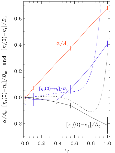
Figure 1: Dependencies of $\alpha$ (red solid line), $\eta_{\mathrm{t}}(0)-\eta_{\mathrm{t}}$ (blue solid line) and $\kappa_{\mathrm{t}}(0)-\kappa_{\mathrm{t}}$ (black solid line) on the fraction $\epsilon_{\rm f}$ of the kinetic helicity, where $\eta_{\mathrm{t}}(0)=\eta_{\mathrm{t}}(\epsilon_{\rm f}=0)$ and $\kappa_{\mathrm{t}}(0)=\kappa_{\mathrm{t}}(\epsilon_{\rm f}=0)$. Here $\alpha$ is normalized by $A_{0}=u_{\rm rms}/3$, and turbulent diffusion coefficients are normalized by $D_{0}=u_{\rm rms}/3k_{\rm f}$, where $k_{\rm f}$ is the forcing wavenumber. The dashed and dotted blue and black curves give the expressions $(1+\epsilon_{\rm f}^{4})^{3}\epsilon_{\rm f}^{2}/3-\epsilon_{\rm f}^{4}$ and $(1+\epsilon_{\rm f}^{4})^{3}\epsilon_{\rm f}^{2}/6-\epsilon_{\rm f}^{4}$ from Equations (23) and (39), respectively. The theoretical results for $\epsilon_{\mathrm{f}}\gtrsim 0.85$ are shown as dotted lines, because they may not be reliable.

5 Comparisons with numerical results

As in Brandenburg et al. (2025), we compute a turbulent velocity field by solving the fully compressible momentum equation with an isothermal equation of state. In the papers by Brandenburg et al. (2017) and Brandenburg et al. (2025), only fully helical cases were compared with the nonhelical cases. Here, we also compute cases with intermediate kinetic helicities of the forcing. This is accomplished by adding a fraction $\sigma ik_{p}\epsilon_{ijp}f_{j}$ to the nonhelical forcing function $f_{i}$. The fractional helicity is then $\epsilon_{\rm f}=2\sigma/(1+\sigma^{2})$.

We compute the turbulent transport coefficient $\alpha$, $\eta_{\mathrm{t}}$, and $\kappa_{\mathrm{t}}$ in Equations (19) and (36) from the turbulent velocity field discussed above. We use the test-field method (Schrinner et al., 2005, 2007; Brandenburg, 2005; Brandenburg et al., 2008), where we solve numerically the equations for the fluctuating magnetic and passive scalar fields. These are nonlinear inhomogeneous equations, in which the product of the mean magnetic and passive scalar fields act as an inhomogeneous source term. Thus, the test-field equations are different from the original evolution equations, which are homogeneous. Moreover, the mean magnetic and passive scalar fields are not solutions to these equations, but consist of a set of mutually orthogonal fields that are called test fields. They are constructed such that we can compute the desired transport coefficient exactly and not as a fit or by some regression method (Brandenburg & Sokoloff, 2002; Simard et al., 2016; Bendre et al., 2024).

The resulting turbulent transport coefficients depend on time and one or two space coordinates (here only on $z$, in addition to $t$). We are usually interested in their averaged values. To determine error bars, we also compute averages for any one third of the full time series. The results are plotted in Figure 1. As in Brandenburg et al. (2025), we present our results for $\alpha$, $\eta_{\mathrm{t}}$, and $\kappa_{\mathrm{t}}$ in normalized form and divide $\alpha$ by $A_{0}=u_{\mathrm{rms}}/3$ and $\eta_{\mathrm{t}}$ and $\kappa_{\mathrm{t}}$ by $D_{0}=u_{\mathrm{rms}}/3k_{\mathrm{f}}$. Note that $\eta_{\mathrm{t}}(0)=\kappa_{\mathrm{t}}(0)=D_{0}$.

We see that $\alpha$ increases approximately linearly with $\epsilon_{\mathrm{f}}$. For $\eta_{\mathrm{t}}$ and $\kappa_{\mathrm{t}}$, it is convenient to plot the differences from the nonhelical values, $\eta_{\mathrm{t}}(0)$ and $\kappa_{\mathrm{t}}(0)$, respectively. We see that for both functions, the differences are small when $\epsilon_{\mathrm{f}}\lesssim 0.4$, and then depart from zero in opposite directions. This is also predicted by the theory. For $\epsilon_{\mathrm{f}}\gtrsim 0.85$, however, there are major departures between our theory and the simulations of Brandenburg et al. (2025) for $\epsilon_{\mathrm{f}}=1$. Note that the simulations (Brandenburg et al., 2025) predict similar results both for passive scalars using the test-field method and for active scalars based on the decay of an initial entropy perturbation.

The strong dependence of the theoretical results from Equations (23) and (39) involving high powers of $\epsilon_{\mathrm{f}}$ is related to the following reasons. The main contributions to the difference in turbulent diffusion coefficients for helical and non-helical turbulence come from the fourth-order moments of a random velocity field. The second reason for the high powers of $\epsilon_{\mathrm{f}}$ in turbulent diffusion coefficients is related to the strong dependence of the correlation time of a random velocity field on $\epsilon_{\mathrm{f}}$ found in simulations (Brandenburg et al., 2025). The difference between the theoretical predictions and the simulations (Brandenburg et al., 2025) for $1\geq\epsilon_{\mathrm{f}}>0.85$ is related to the theory being based on the assumptions: (i) the contributions of higher than fourth-order moments of a random velocity field are neglected; (ii) it is assumed that the velocity field has Gaussian statistics; and (iii) we use a model of a random velocity field with renovations.

6 Discussion

One of the main effects of astrophysical turbulent flows is a strong increase of the diffusion of the large-scale magnetic and scalar fields, which can be characterized in terms of the effective (turbulent) diffusion coefficients. The latter effect decreases the growth rates of the mean-field dynamo instability and various clustering instabilities related to scalar fields.

In the present study, we have developed a theory which explains the nontrivial behavior of turbulent diffusion coefficients of the large-scale magnetic and scalar fields as functions of the kinetic helicity. These effects have been recently discovered by direct numerical simulations (Brandenburg et al., 2017, 2025), which show that turbulent magnetic diffusion decreases with increasing kinetic helicity while turbulent diffusion of passive scalars increases with the helicity. The main contribution to these effects comes from the fourth-order correlation function of the turbulent velocity field. This is the reason why widely used methods like the quasi-linear approach [the first-order smoothing approximation (FOSA) or the second-order correlation approximation (SOCA)] as well as the various $\tau$ approaches and the direct interaction approximation (DIA) cannot describe these effects.

In the present study, we have applied the path-integral approach for random flows with a finite correlation time and for large Reynolds and Péclet numbers. We have assumed that the velocity field has Gaussian statistics, which allows us to represent the fourth-order moments of the turbulent velocity field as a product of second-order moments. A crucial role in the understanding of these effects is played by the kinetic helicity effect on the turbulent correlation time, which increases with increasing helicity. The results of the theory developed here are in agreement with the numerical results of Brandenburg et al. (2017, 2025).

References

- Bendre et al. (2024) Bendre, A. B., Schober, J., Dhang, P., & Subramanian, K. 2024, MNRAS, 530, 3964, doi: 10.1093/mnras/stae1100
- Brandenburg (2005) Brandenburg, A. 2005, Astron. Nachr., 326, 787, doi: 10.1002/asna.200510414
- Brandenburg et al. (2025) Brandenburg, A., Käpylä, P. J., Rogachevskii, I., & Yokoi, N. 2025, ApJ, submitted, arXiv:2501.08879
- Brandenburg et al. (2008) Brandenburg, A., Rädler, K.-H., & Schrinner, M. 2008, A&A, 482, 739, doi: 10.1051/0004-6361:200809365
- Brandenburg et al. (2017) Brandenburg, A., Schober, J., & Rogachevskii, I. 2017, Astron. Nachr., 338, 790, doi: 10.1002/asna.201713384
- Brandenburg & Sokoloff (2002) Brandenburg, A., & Sokoloff, D. 2002, Geophysical and Astrophysical Fluid Dynamics, 96, 319, doi: 10.1080/03091920290032974
- Dittrich et al. (1984) Dittrich, P., Molchanov, S. A., Sokolov, D. D., & Ruzmaikin, A. A. 1984, Astron. Nachr., 305, 119, doi: 10.1002/asna.2113050305
- Elperin et al. (2000) Elperin, T., Kleeorin, N., Rogachevskii, I., & Sokoloff, D. 2000, Phys. Rev. E, 61, 2617, doi: 10.1103/PhysRevE.61.2617
- Elperin et al. (2001) —. 2001, Phys. Rev. E, 64, 026304, doi: 10.1103/PhysRevE.64.026304
- Kleeorin et al. (2002) Kleeorin, N., Rogachevskii, I., & Sokoloff, D. 2002, Phys. Rev. E, 65, 036303, doi: 10.1103/PhysRevE.65.036303
- Krause & Rädler (1980) Krause, F., & Rädler, K.-H. 1980, Mean-Field Magnetohydrodynamics and Dynamo Theory (Oxford: Pergamon Press)
- Lamburt et al. (2000) Lamburt, V. G., Sokoloff, D. D., & Tutubalin, V. N. 2000, Astron. Rep., 44, 659, doi: 10.1134/1.1312962
- Mizerski (2023) Mizerski, K. A. 2023, Phys. Rev. E, 107, 055205, doi: 10.1103/PhysRevE.107.055205
- Moffatt (1978) Moffatt, H. K. 1978, Magnetic Field Generation in Electrically Conducting Fluids (Cambridge: Cambridge University Press)
- Moffatt & Dormy (2019) Moffatt, H. K., & Dormy, E. 2019, Self-Exciting Fluid Dynamos (Cambridge Univ. Press, Cambridge), doi: 10.1017/9781107588691
- Nicklaus & Stix (1988) Nicklaus, B., & Stix, M. 1988, Geophys. Astrophys. Fluid Dynam., 43, 149, doi: 10.1080/03091928808213623
- Parker (1979) Parker, E. N. 1979, Cosmical Magnetic Fields: Their Origin and Their Activity (Oxford: Clarendon Press)
- Pouquet & Yokoi (2022) Pouquet, A., & Yokoi, N. 2022, Phil. Trans. Roy. Soc. Lond. Ser. A, 380, 20210087, doi: 10.1098/rsta.2021.0087
- Rogachevskii (2021) Rogachevskii, I. 2021, Introduction to turbulent transport of particles, temperature and magnetic fields: analytical methods for physicists and engineers (Cambridge University Press), doi: 10.1063/5.0188732,2024
- Rüdiger et al. (2013) Rüdiger, G., Kitchatinov, L. L., & Hollerbach, R. 2013, Magnetic Processes in Astrophysics: Theory, Simulations, Experiments (John Wiley and Sons, Weinheim), doi: 10.1002/9783527648924
- Ruzmaikin et al. (1988) Ruzmaikin, A., Shukurov, A., & Sokoloff, D. 1988, Magnetic Fields of Galaxies (Dordrecht: Kluwer)
- Schrinner et al. (2005) Schrinner, M., Rädler, K.-H., Schmitt, D., Rheinhardt, M., & Christensen, U. 2005, Astron. Nachr., 326, 245, doi: 10.1002/asna.200410384
- Schrinner et al. (2007) Schrinner, M., Rädler, K.-H., Schmitt, D., Rheinhardt, M., & Christensen, U. R. 2007, Geophys. Astrophys. Fluid Dynam., 101, 81, doi: 10.1080/03091920701345707
- Shukurov & Subramanian (2022) Shukurov, A., & Subramanian, K. 2022, Astrophysical Magnetic Fields: From Galaxies to the Early Universe (Cambridge: Cambridge University Press)
- Simard et al. (2016) Simard, C., Charbonneau, P., & Dubé, C. 2016, Advances in Space Research, 58, 1522, doi: 10.1016/j.asr.2016.03.041
- Zeldovich et al. (1990) Zeldovich, Y. B., Ruzmaikin, A. A., & Sokoloff, D. D. 1990, The Almighty Chance (Singapore: World Scientific)
- Zeldovich et al. (1983) Zeldovich, Ya. B., Ruzmaikin, A. A., & Sokoloff, D. D. 1983, Magnetic Fields in Astrophysics (New York: Gordon and Breach)