Inference for generalized additive mixed models via penalized marginal likelihood

Abstract

Existing methods for fitting generalized additive mixed models to longitudinal repeated measures data rely on Laplace-approximate marginal likelihood for estimation of variance components and smoothing penalty parameters. This is thought to be appropriate due to the Laplace approximation being established as an appropriate tool for smoothing penalty parameter estimation in spline models and the well-known connection between penalized regression and random effects. This paper argues that the Laplace approximation is sometimes not sufficiently accurate for smoothing parameter estimation in generalized additive mixed models leading to estimates that exhibit increasing bias and decreasing confidence interval coverage as more groups are sampled. A novel estimation strategy based on penalizing an adaptive quadrature approximate marginal likelihood is proposed that solves this problem and leads to estimates exhibiting the correct statistical properties.

1 Introduction

A generalized additive mixed model for a response $y=(y_{1}^{\rm{T}},\ldots,y_{m}^{\rm{T}})^{\rm{T}}\in\mathbb{R}^{n}$ where each $y_{i}=(y_{i1},\ldots,y_{in_{i}})^{\rm{T}}\in\mathbb{R}^{n_{i}}$ with $n=n_{1}+\cdots+n_{m}$ is:

$$y_{ij}|u_{i}\overset{ind}{\sim}\Psi\{\mu(x_{ij},u_{i})\},\ \mu(x,u)=\sum_{s=1}^{p}f_{s}(x_{s})+u,\ u_{i}\overset{iid}{\sim}N\left(0,\sigma^{2}\right).$$ (1)

Here $x_{ij}\in\mathbb{R}^{p}$ for $i=1,\ldots,m,j=1,\ldots,n_{i}$, $u_{i}\in\mathbb{R}$, and $\Psi$ is a distribution having suitably smooth density $\psi$. The random effects $u_{i},i=1,\ldots,m$ induce dependence between observations $y_{ij},y_{il}$ in the same group. The unknown smooth functions $f_{1},\ldots,f_{p}$ allow the mean to depend on the covariates in a nonlinear manner and are represented by the basis expansions

$$f_{s}(x)=\sum_{l=1}^{d_{s}}b_{ls}(x)\beta_{ls},$$

where $b_{ls}$ is the $l$th cubic B-spline basis function for function $f_{s}$ on a knot sequence of appropriate length, and $\beta_{ls}$ is the corresponding spline weight to be estimated from the data. The full vector of $d=d_{1}+\cdots+d_{p}$ unknown spline weights is $\beta=(\beta_{1}^{\rm{T}},\ldots,\beta_{p}^{\rm{T}})^{\rm{T}}\in\mathbb{R}^{d}$ where $\beta_{s}=(\beta_{s1},\ldots,\beta_{sd_{s}})^{\rm{T}}$. Estimation of $\beta$ and prediction of $u$ is based on minimizing the negative penalized log-likelihood,

$$\mathcal{L}(u,\beta;y,\theta) =\sum_{i=1}^{m}\mathcal{L}_{i}(u_{i},\beta;y,\theta)+\mathcal{P}(\beta,\lambda),$$ (2)

$$=-\sum_{i=1}^{m}\left[\sum_{j=1}^{n_{i}}\log\psi\{y_{ij};\mu(x_{ij},u_{i})\}+\log g(u_{i};\sigma)\right]+\sum_{s=1}^{p}\left[\frac{\lambda_{s}}{2}\int\left\{f^{\prime\prime}_{s}(x)\right\}^{2}dx-\log\lambda_{s}\right],$$ (3)

(Wood, 2011; Wood et al., 2013), where $\theta=(\sigma,\lambda_{1},\ldots,\lambda_{p})^{\rm{T}}\in\mathbb{R}^{p+1}$ contains the random effect variance and smoothing penalty parameters, both of which must be estimated, and $g(u;\sigma)$ is the density of $u\sim\text{N}(0,\sigma^{2})$. A connection between penalized smoothing and random effects models is observed by writing the penalty as a quadratic form in $\beta$,

$$\int\left\{f^{\prime\prime}_{s}(x)\right\}^{2}dx=\beta_{s}^{\rm{T}}S_{s}\beta_{s},\ \left(S_{s}\right)_{lr}=\int b^{\prime\prime}_{ls}(x)b^{\prime\prime}_{rs}(x)dx,\ \text{dim}(S_{s})=d_{s},\ \text{rank}(S_{s})=d_{s}-2,$$

and hence interpreting it as an improper Gaussian prior on $\beta$ with precision matrix $S_{\lambda}=\text{blockdiag}(\lambda_{1}S_{1},\ldots,\lambda_{p}S_{p})$. It follows that $\exp\{-\mathcal{P}(\beta,\lambda)\}$ is proportional to a (low rank) Gaussian density with precision matrix $S_{\lambda}$, and hence $\mathcal{L}$ is a negative joint log-likelihood of $u,\beta$. Interpreting the penalized smooths as random effects leads to inference for $\theta$ based on minimizing the negative marginal log-likelihood (Wood, 2011),

$$\mathcal{M}(\theta;y)=-\log\int\exp\left\{-\mathcal{L}(u,\beta;y,\theta)\right\}dud\beta,$$ (4)

so $\widehat{\theta}=\text{argmin }\mathcal{M}(\theta;y)$. However, when $\Psi$ is not a Gaussian distribution, the integral (4) is intractable and $\widehat{\theta}$ cannot be calculated. Instead, inference is based on minimizing some approximation to $\mathcal{M}$. Current methods in the literature (Wood et al., 2013) and in software (package mgcv, Wood 2011 and package gamm4, Wood and Scheipl 2020) employ the Laplace approximation for this purpose,

$$\widetilde{\mathcal{M}}_{LA}(\theta;y)=-\frac{m+d}{2}\log(2\pi)+\frac{1}{2}\log\det\{H(\theta)\}-\mathcal{L}\{\widehat{u}(\theta),\widehat{\beta}(\theta);y,\theta\},$$ (5)

where $\widehat{u}(\theta)=\text{argmin}_{u}\mathcal{L}(u,\beta;y,\theta)$, $\widehat{\beta}(\theta)=\text{argmin}_{\beta}\mathcal{L}(u,\beta;y,\theta)$, and $H(\theta)$ is the Hessian of $\mathcal{L}$ with respect to $u,\beta$ at $\widehat{u}(\theta),\widehat{\beta}(\theta)$ for given $\theta$. While the Laplace approximation is known to be acceptable for smoothing penalty parameter estimation in spline models without group-specific random effects (Kauermann et al., 2009), it is often not sufficiently accurate for variance component estimation in generalized linear mixed models with group-specific random effects (Joe, 2008; Kim et al., 2013; Stringer, 2025; Bilodeau et al., 2025). The use of the Laplace approximation for variance in generalized additive mixed models has not been directly investigated, but these analyses for the linear case suggest that it may not be appropriate. To see the potential problem, observe that the marginal likelihood factors in the following manner:

$$\exp\left\{-\mathcal{M}(\theta;y)\right\}=\int\left[\prod_{i=1}^{m}\int\exp\left\{-\mathcal{L}_{i}(u_{i},\beta;y,\theta)\right\}du_{i}\right]\exp\left\{-\mathcal{P}(\beta,\lambda)\right\}d\beta.$$ (6)

Inspection of (6) reveals that the $du$ integral in (4) factors over $u_{1},\ldots,u_{m}$ due to their assumed independence. However, $m\to\infty$ is required for consistency of $\widehat{\theta}$, which is in turn required for consistency of $\widehat{\beta}$. For generalized linear mixed models Ogden (2017) gives a thorough analysis of lower bounds and argues that $m$ cannot grow too fast compared to $n_{\text{min}}$ if consistent estimates are desired. Figure 3 in section 3 shows the coverage of confidence intervals for $f$ decreasing as $m$ is increased in a simulated example, illustrating the practical failure of the Laplace approximation. Bilodeau et al. (2025); Stringer (2025) show futher simulations and provide a stochastic upper bound on the error in using adaptive Gaussian quadrature to fit generalized linear mixed models which shows that using this more accurate integral approximation mitigates the problem. Unfortunately, in generalized additive mixed models, while adaptive quadrature could be applied to each one-dimensional $du_{i}$ integral, the dimension of the $d\beta$ integral is too large for this technique to be computationally feasible.

2 A two-stage approach to inference in generalized additive mixed models

We propose to ignore dependence between the observations for the purposes of smoothing parameter estimation, which we address using a standard generalized additive model fit by Laplace-approximate marginal likelihood or restricted marginal likelihood. We then propose to fit a generalized linear mixed model with a fixed penalty for $\beta$, using the estimated smoothing parameters from the first step. This follows the common practice of ignoring uncertainty in the estimation of $\lambda_{1},\ldots,\lambda_{p}$, but adequately captures the uncertainty in $\beta$ and hence $f$, leading to confidence intervals whose coverages appear to attain the nominal level as $m\to\infty$.

First consider the generalized additive model,

$$y_{ij}\overset{ind}{\sim}\Psi\{\mu(x_{ij})\},\ \mu(x)=\sum_{s=1}^{p}f_{s}(x_{s}),$$ (7)

which is Eq. (1) with $\sigma=0$. This model is fit by employing the Laplace-approximate marginal or restricted marginal likelihood method of Wood (2011) through the mgcv package. Let $\widehat{\lambda}=(\widehat{\lambda}_{1},\ldots,\widehat{\lambda}_{p})^{\rm{T}}$ be the estimated smoothing parameters obtained in this manner, and let $S_{\widehat{\lambda}}=\text{blockdiag}(\widehat{\lambda}_{1}S_{1},\ldots,\widehat{\lambda}_{p}S_{p})$. Let $z\in Q(k)\subset\mathbb{R}^{+}\cup\{0\}$ be the points and $w_{k}:Q(k)\to\mathbb{R}^{+}$ the weights from a Gauss-Hermite quadrature rule of order $k$ (Bilodeau et al., 2024, Eqs. 3 and 4), $\widehat{u}_{i}\equiv\widehat{u}_{i}(\sigma,\beta)=\text{argmin}_{u}\mathcal{L}_{i}(u,\beta;y,\sigma,\widehat{\lambda})$, and $h_{ii}\equiv h_{ii}(\sigma,\beta)=\partial^{2}_{u^{2}}\mathcal{L}_{i}\{u(\sigma,\beta),\beta;y,\sigma,\widehat{\lambda}\}$. We propose the following penalized approximate log-marginal likelihood for estimating $\sigma,\beta$:

$$\exp\left\{-\widetilde{\mathcal{M}}_{k}(\sigma,\beta)\right\}=\left[\prod_{i=1}^{m}h_{ii}^{-1/2}\sum_{z\in Q(k)}w_{k}(z)\mathcal{L}_{i}\{\widehat{u}_{i}+z\cdot h_{ii}^{-1/2},\beta;y,\lambda\}\right]\exp\left\{-\mathcal{P}(\beta,\widehat{\lambda})\right\}.$$ (8)

We estimate $(\widehat{\sigma},\widehat{\beta})^{\rm{T}}=\text{argmin }\widetilde{\mathcal{M}}_{k}(\sigma,\beta)$ and form Wald confidence intervals for $\beta$ using standard errors obtained as the appropriate diagonal elements of the inverse Hessian of $\widetilde{\mathcal{M}}_{k}(\widehat{\sigma},\widehat{\beta})$.

The accuracy of the approximation (8) is determined by the order of the quadrature rule, $k\in\mathbb{N}$. In generalized linear and non-linear mixed models, Bilodeau et al. (2025) show that under assumptions on the model that include the exponential family, for any $\varepsilon>0$ if $m=n_{min}^{q}$ for some $q>0$ then the relative approximation error is $O_{p}[R_{n}n_{min}^{-\{r(k)+1\}/2+\varepsilon}]$ where $r(k)=\lfloor(k+2)/3\rfloor$ and $R_{n}=m^{1/2}$ or $(mn)^{1/2}$ is the parameter-dependent rate of convergence of the maximum likelihood estimator based on the exact marginal likelihood (Jiang et al., 2022). For fixed $\beta$ this result is expected to apply here without modification, since all that is changed is the addition of the $\exp\{-\mathcal{P}(\beta,\widehat{\lambda})\}$ term which does not depend on $m,n$. The practical implication, as discussed by Bilodeau et al. (2025), is that $k$ can always be chosen high enough for a given set of data such that the sampling error in $y$ dominates the numerical error in the integral approximation, rendering inferences indistinguishable from those that would be obtained if the exact marginal likelihood could be calculated.

3 Empirical Analysis

A simulation study was conducted to (a) illustrate the inadequacy of Eq. (5) for inferences in the generalized additive mixed model (1), and (b) provide empirical evidence of the adequacy of the proposed penalized marginal likelihood given by Eq. (8) for these inferences. Code for reproducing these results is available at https://github.com/awstringer1/gamm-paper-code.

Computation of $(\widehat{\sigma},\widehat{\beta})^{\rm{T}}$ is by gradient-based quasi-Newton optimization. Stringer (2025) provides an algorithm for computing the exact gradient of $\widetilde{\mathcal{M}}_{k}(\sigma,\beta)$ without the $\mathcal{P}(\beta,\widehat{\lambda})$ term. The gradient of that term with respect to $\beta$ is trivial to obtain and computation therefore proceeds via the appropriate minor modification to the method and software of Stringer (2025). The Laplace-approximate generalized additive mixed model was implemented using the Template Model Builder (Kristensen et al., 2016, R package TMB) and the generalized additive model is fit using the R package mgcv (Wood, 2011).

Replicate sets of data with equal-sized groups were generated from model (1) with $p=1,f(x)=\sin(2\pi x),\sigma=1$, and varying $m,n$. To each of the simulated data sets, the model (1) was fit using (a) a standard generalized additive model that ignores dependence in $y$ (GAM), (b) the existing method by minimizing $\widetilde{\mathcal{M}}_{LA}(\theta;y)$ (GAMM), and (c) the new penalized marginal likelihood method described in section 2, with $k=9$ quadrature points (PML). The bias in $f$ and $\sigma$ are reported and the average across-the-function coverage in $f$ is compared to the nominal value of $95\%$. To make the reported mean coverage percentages accurate to within roughly 1 decimal place, $1,000$ simulated data sets were generated.

The results are shown in Figures 1 – 3. Figure 1 shows that all three approaches are successful at point estimation of $f$, having zero average empirical bias for all values of $m$ and $n$ considered. Figure 3 shows empirical coverages. The generalized additive model has empirical coverage that drops substantially as both $m$ and $n$ are increased, which is expected as this model incorrectly ignores dependence in $y$. The Laplace-approximate generalized additive mixed model captures dependence in $y$, but still has empirical coverage that decreases as $m$ is increased. In contrast to the generalized additive model, this behaviour is less severe when $n$ is larger. The explanation is that this behaviour is due to the inadequacy of the Laplace approximation due to the factoring of the marginal likelihood into a product of $m$ integrals with each integrand depending on $n$ data points. As $n$ is increased, each of the $m$ Laplace approximations become more accurate but as $m$ is increased, errors multiply and the approximation to the whole likelihood becomes less accurate. The same phenomenon is reported by Stringer (2025) and Bilodeau et al. (2025), the latter of which offers a rigorous theoretical explanation. In contrast, the penalized marginal likelihood approach exhibits nominal average coverage for all values of $m$ and $n$ tried, since it relies on an appropriately accurate approximation to the marginal likelihood and incorporates appropriate penalization of $\beta$. Finally, Figure 2 shows empirical bias for estimation of $\sigma$ from the generalized additive mixed model and penalized marginal likelihood. The generalized additive model sets $\sigma=0$ so does not return an estimate. The generalized additive mixed model shows bias converging to a nonzero value as $m$ is increased for both values of $n$, with the effect less severe for larger $n$. The penalized marginal likelihood again corrects this behaviour with empirical bias converging to zero as $m$ is increased, and smaller bias for larger $n$.

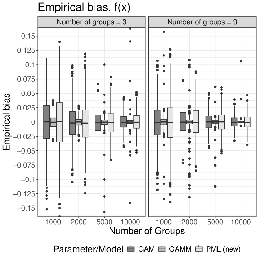
Figure 1: Empirical bias in estimated $f$ across $1,000$ simulations. Despite the GAM ignoring dependence and the GAMM using an insufficiently accurate approximation to the marginal likelihood, all three methods exhibit zero average bias, with decreasing variability as either more or larger groups are obtained.

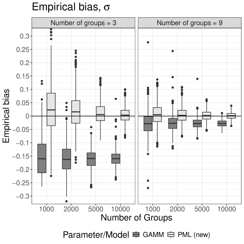
Figure 2: Empirical bias in estimated $\sigma$ across $1,000$ simulations. The GAM does not estimate $\sigma$. The GAMM uses an insufficiently accurate Laplace approximation for inference, and shows substantial bias which appears to converge to a nonzero value for increasing $m$; the effect is weaker for larger $n$. The new PML approach exhibits the correct behaviour of bias converging to zero as $m$ increases.

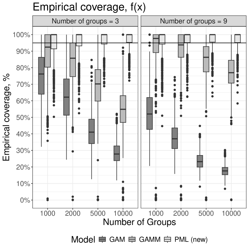
Figure 3: Empirical coverage in estimated $f(x)$ across $1,000$ simulations. The GAM ignores dependence and exhibits decreasing coverage as the number of groups, $m$, increases. The GAMM accounts for dependence but uses an insufficiently accurate Laplace approximation for inference, and exhibits decreasing coverage for increasing $m$; the effect is weaker for larger $n$. The new PML approach exhibits nominal coverage for all values of $m$ and $n$.

References

- Bilodeau et al. (2024) Bilodeau, B., A. Stringer, and Y. Tang (2024). Stochastic convergence rates and applications of adaptive quadrature in bayesian inference. Journal of the American Statistical Association 119(545), 690–700.
- Bilodeau et al. (2025) Bilodeau, B., A. Stringer, and Y. Tang (2025+). Asymptotics of numerical integration for two-level mixed models. Submitted.
- Jiang et al. (2022) Jiang, J., M. P. Wand, and A. Bhaskaran (2022). Usable and precise asymptotics for generalized linear mixed model analysis and design. Journal of the Royal Statistical Society Series B: Statistical Methodology 84(1), 55–82.
- Joe (2008) Joe, H. (2008). Accuracy of Laplace Approximation for Discrete Response Mixed Models. Computational Statistics and Data Analysis 52, 5066–5074.
- Kauermann et al. (2009) Kauermann, G., T. Krivobokova, and L. Fahrmeir (2009). Some asymptotic results on generalized penalized spline smoothing. Journal of the Royal Statistical Society Series B: Statistical Methodology 71(2), 487–503.
- Kim et al. (2013) Kim, Y., Y.-K. Choi, and S. Emery (2013). Logistic regression with multiple random effects: A simulation study of estimation methods and statistical packages. The American Statistician 67(3), 171–182.
- Kristensen et al. (2016) Kristensen, K., A. Nielson, C. W. Berg, H. Skaug, and B. M. Bell (2016). TMB: automatic differentiation and Laplace approximation. Journal of statistical software 70(5).
- Ogden (2017) Ogden, H. (2017). On asymptotic validity of naive inference with an approximate likelihood. Biometrika 104(1).
- Stringer (2025) Stringer, A. (2025). Exact gradient evaluation for adaptive quadrature approximate marginal likelihood in mixed models for grouped data. Statistics and Computing 35(4).
- Wood (2011) Wood, S. (2011). Fast stable restricted maximum likelihood and marginal likelihood estimation of semiparametric generalized linear models. Journal of the Royal Statistical Society, Series B (Statistical Methodology) 73(1), 3 – 36.
- Wood and Scheipl (2020) Wood, S. and F. Scheipl (2020). gamm4: Generalized Additive Mixed Models using ’mgcv’ and ’lme4’. R package version 0.2-6.
- Wood et al. (2013) Wood, S., F. Scheipl, and J. Faraway (2013). Straightforward intermediate rank tensor product smoothing in mixed models. Statistics and Computing 23, 341–360.