Ab initio modeling of single-photon detection in superconducting nanowires

Abstract

Using a kinetic equation approach and Density Functional Theory, we model the nonequilibrium quasiparticle and phonon dynamics of a thin superconducting film under optical irradiation ab initio. We extend this model to develop a theory for the detection of single photons in superconducting nanowires. In doing so, we create a framework for exploring new superconducting materials for enhanced device performance beyond the state-of-the-art. Though we focus in this study on superconducting nanowire single-photon detectors, these methods are general, and they can be extended to model other superconducting devices, including transition-edge sensors, microwave resonators, and superconducting qubits. Our methods effectively integrate ab initio materials modeling with models of nonequilibrium superconductivity to perform practical modeling of superconducting devices, providing a comprehensive approach that connects fundamental theory with device-level applications.

The success of the Migdal-Eliashberg theory has illustrated the importance of considering the full-bandwidth electron-phonon coupling spectrum to describe conventional superconductivity [1, 2, 3]. This theory not only provides insights into equilibrium superconductivity but also lays the foundation for understanding nonequilibrium phenomena, where the electron-phonon coupling determines the evolution of the quasiparticle and phonon distributions. These distributions, in turn, influence the modification of the transport properties of a material when subjected to external perturbations, such as radiation absorption or heating [4, 5, 6, 7]. However, obtaining the full-bandwidth electron-phonon coupling spectrum for arbitrary materials has historically been difficult. Thus, studies of the nonequilibrium dynamics of superconductors typically rely on approximating the phonon system with a Debye model [7, 8, 9]. This approximation, which assumes a linear dispersion for the phonons, is generally inadequate for capturing realistic electron-phonon coupling. Therefore, this approximation can only provide qualitative predictions and cannot be used to describe general nonequilibrium superconductivity.

This limitation of the Debye model is a critical issue for device modeling, as nonequilibrium dynamics are central to the operation of many superconducting devices. One such device is the superconducting nanowire single-photon detector (SNSPD), which has earned widespread recognition due to its exceptional performance characteristics, including near-unity internal single-photon detection efficiency [10, 11, 12], single-photon sensitivity in the visible to mid-infrared wavelengths [13, 14], ultra-low dark-count rates [15, 16], and sub-$3\text{\,}\mathrm{ps}$ timing jitter [17]. However, applications including dark-matter search, biomedical imaging, particle detection, and space communication can benefit considerably from improvements in the operating temperature and wavelength sensitivity of these detectors. This possibility has led to a significant effort to explore new materials for SNSPDs [18, 19, 20, 21], and engineer existing SNSPD material platforms for enhanced device performance [17, 12, 14]. To direct this effort, a precise understanding of the physical mechanism underpinning photon detection in SNSPDs is required. This need has led the photon detection process to be the subject of intense study for the last two decades [22, 23, 24, 25, 26, 27, 28, 29, 30]. For this reason, we direct our efforts in this work towards developing a model for photon detection in superconducting nanowires.

To this end, several phenomenological models of photon detection in superconducting nanowires have been proposed; however, these models are generally unsatisfactory for describing arbitrary SNSPD geometries and materials. Prior work has demonstrated the crucial role of quasiparticle and phonon interactions in the initial stages of photon detection [25, 26, 28, 30, 31], but only a limited number of studies have attempted to model these interactions directly [25, 28, 30]. Moreover, studies incorporating these interactions have relied on a Debye model and consequently have neglected the effect of realistic electron-phonon coupling.

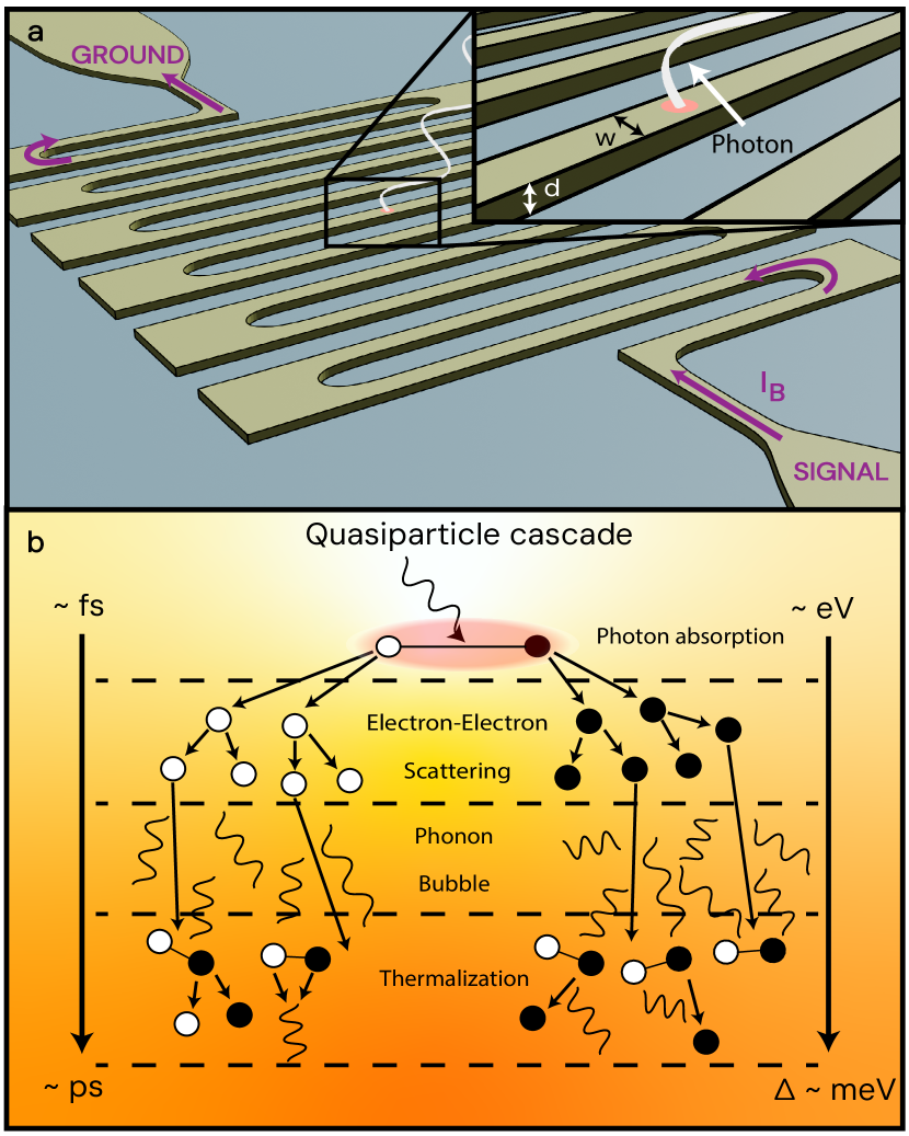
Figure 1: High-level overview of the superconducting nanowire single-photon detector (SNSPD) detection mechanism. (a) Typical SNSPD geometry, consisting of a thin ($d\sim\xi_{\mathrm{c}}$) narrow ($w\ll\Lambda$) superconducting wire that is patterned in a meander to increase the active area of the detector. The device is single-photon sensitive when a bias current $I_{\mathrm{B}}$ near the critical current of the wire is applied. (b) Microscopic picture of SNSPD detection. A photon is absorbed generating an excited quasiparticle consisting of an electron-hole pair. The relaxation of this quasiparticle triggers an energy-relaxation cascade and the generation of a phonon bubble. The resulting quasiparticles and phonons scatter and break pairs, locally suppressing the superconductivity and weakening the barrier so that quantum and thermal fluctuations can fully destroy the superconductivity across the strip. Due to the bias current, this normal strip produces a nonzero voltage across the terminals of the device which is read out as a detection event.

To overcome these limitations, we develop an ab initio model to quantitatively predict the microscopic response of a thin narrow superconducting wire to external perturbation. To do so, we employ recent advances in ab initio materials modeling within the framework of Density Functional Perturbation Theory (DFPT) that have made it possible to accurately calculate the full-bandwidth electron-phonon coupling for a wide range of conventional superconductors [32, 33]. The result is a model that can predict nonequilibrium quasiparticle and phonon dynamics in a conventional superconductor, which is of interest for developing and studying superconducting detectors [28, 30], microwave resonators [34], and quasiparticle poisoning of qubits [35, 36]. In this work, we apply this model to describe a film irradiated by optical photons and describe the photon-detection mechanism of SNSPDs. We then predict the wavelength sensitivity of an SNSPD by determining the detection current $I_{\mathrm{det}}$, defined as the current at which the internal detection efficiency of an SNSPD saturates for a given photon wavelength and device temperature, and compare our results to experimental data. We focus on niobium nitride ($\mathrm{NbN}$) due to its relevance as a material for SNSPD fabrication; however, the methods outlined here are suitable to describe any conventional isotropic superconductor and can be generalized to incorporate anisotropy [4]. We also emphasize that as an ab initio theory, the predictions of this model are based on first-principles calculations of the material’s properties and can be made with no experimental input.

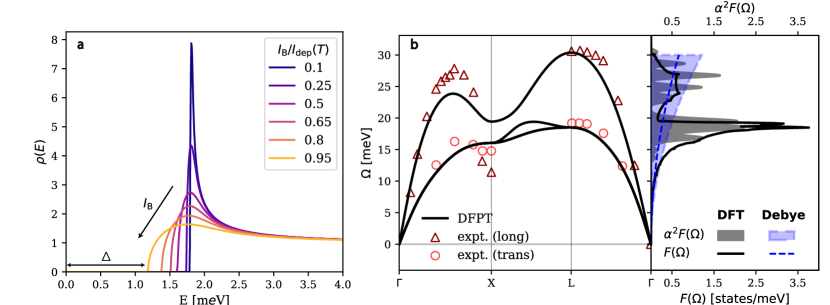
Figure 2: (a) Normalized quasiparticle density of states $\rho(E)$ for $\delta$-$\mathrm{NbN}$ with $T_{\mathrm{c}}=10\,\mathrm{K}$ and different ratios of the bias current normalized to the depairing current $I_{\mathrm{B}}/I_{\mathrm{dep}}(T)$. (b) Acoustic phonon modes for $\delta$-$\mathrm{NbN}$ calculated using Density Functional Perturbation Theory compared to experimental data for the longitudinal and transverse modes [37]. The corresponding Eliashberg spectral function $\alpha^{2}F(\Omega)$ (solid grey) and phonon density of states $F(\Omega)$ (black) are displayed on the right compared to the Debye approximation (dashed and solid blue).

For this study, we consider a typical SNSPD geometry, consisting of a thin, narrow superconducting film that has absorbed a single optical photon while carrying a nonzero bias current $I_{\mathrm{B}}$. As depicted in Fig. 1a, such a film is characterized by a thickness on the order of the superconducting coherence length $d\sim\xi_{\mathrm{c}}=\sqrt{\hbar D/|\Delta|}$ and width much smaller than the Pearl length $w\ll\Lambda=2\lambda_{\mathrm{L}}^{2}/d$, where $\lambda_{\mathrm{L}}$ is the London penetration depth ($\lambda_{\mathrm{L}}=\sqrt{\hbar\rho_{\rm{N}}/\mu_{0}\pi|\Delta|}$), $\rho_{\rm{N}}$ is the normal state resistivity ($\rho_{\mathrm{N}}=1/2e^{2}DN(0)$), $e$ is the electron charge, $N(0)$ is the single-spin electron density of states at the Fermi energy $E_{\mathrm{F}}$, $\mu_{0}$ is the permeability of free-space, $\hbar$ is the reduced Planck constant, $D$ is the electronic diffusion coefficient ($D=v_{\mathrm{F}}l_{e}/3$), $v_{\rm F}$ is the Fermi velocity, $l_{e}$ is the electron mean-free path, and $|\Delta|$ is the magnitude of the superconducting order parameter and equal to the leading-edge gap. In general, $|\Delta|$ is a function of temperature $T$, $I_{\mathrm{B}}$, and position $\mathbf{r}$. As discussed later, we will adopt the BCS limit for numerical calculations.

We begin by discussing the initial quasiparticle cascade caused by photon absorption in a superconducting film. We then connect these results to the mesoscopic dynamics of the superconducting order parameter. When a photon is absorbed in the superconducting film, a single quasiparticle is excited with an energy $E_{\lambda}\gg|\Delta|$ as displayed in Fig. 1b. The resulting nonequilibrium dynamics can be described by a set of kinetic equations for the quasiparticle $f(E)$ and phonon $n(\Omega)$ distribution functions, which for an isotropic material are

$$\frac{df(E)}{dt}= -\frac{2\pi}{\hbar}\int_{0}^{\infty}d\Omega\,\alpha^{2}F(\Omega)\rho(E+\Omega)K_{\mathrm{ph}-e}(E,\Omega)$$ (1a)

$$-\frac{2\pi}{\hbar}\int_{0}^{E-|\Delta|}d\Omega\,\alpha^{2}F(\Omega)\rho(E-\Omega)K_{e-\mathrm{ph}}(E,\Omega)$$

$$-\frac{2\pi}{\hbar}\int_{E+|\Delta|}^{\infty}d\Omega\,\alpha^{2}F(\Omega)\rho(\Omega-E)K_{\mathrm{R}}(E,\Omega)$$

and

$$\frac{dn(\Omega)}{dt} =-\frac{8\pi}{\hbar}\frac{N(0)}{N}\int_{|\Delta|}^{\infty}d\!E\int_{|\Delta|}^{\infty}d\!E^{\prime}\,\alpha^{2}(\Omega)\rho(E)\rho(E^{\prime})$$ (1b)

$$\times\Bigg{[}K_{\mathrm{S}}(E,E^{\prime},\Omega)\delta(E+\Omega-E^{\prime})$$

$$+K_{\mathrm{B}}(E,E^{\prime},\Omega)\delta(E+E^{\prime}-\Omega)\Bigg{]}-\frac{n(\Omega)-n^{\mathrm{eq}}(\Omega)}{\tau_{\mathrm{esc}}},$$

where the integral kernels $K_{i}$ are functions of $f(E)$ and $n(\Omega)$ and are defined in the Appendix. $K_{\mathrm{ph}-e}(E,\Omega)$ ($K_{e-\mathrm{ph}}(E,\Omega)$) describes the quasiparticle scattering due to the absorption (emission) of a phonon, while $K_{\mathrm{R}}(E,\Omega)$ represents the quasiparticle recombination process. $K_{\mathrm{S}}(E,E^{\prime},\Omega)$ captures the phonon scattering process, and $K_{\mathrm{B}}(E,E^{\prime},\Omega)$ describes the phonon pair-breaking process. Here, $N$ is the number of ions per unit volume, and $\rho(E)$ is the normalized quasiparticle density of states [7]. For a film in the dirty limit, characterized by $l_{e}\ll\xi_{\mathrm{c}}$, $\rho(E)$ can be calculated for a finite bias current $I_{\mathrm{B}}$ by solving the Usadel equation as detailed in the Appendix. The solutions to the Usadel equaton for $\rho(E)$ are displayed in Fig. 2a. The superconducting order parameter $\Delta$ satisfies

$$|\Delta|=\lambda\int_{|\Delta|}^{\infty}d\!E\,R(E,\Delta)[1-2f(E)],$$ (2)

where $\lambda=2\int_{0}^{\infty}d\Omega\alpha^{2}F(\Omega)/\Omega$ is the electron-phonon coupling parameter and $R(E,\Delta)$ is a spectral function defined in the Appendix [7, 28]. The final term of Eq. (1b) models phonon exchange with the substrate, where $n^{\mathrm{eq}}(\Omega)$ is the usual Bose-Einstein distribution and $\tau_{\mathrm{esc}}$ is the characteristic time for phonon escape to the substrate. To simplify calculations, we ignore the energy dependence of $\tau_{\mathrm{esc}}$.

In Eqs. (1a) and (1b), the quasiparticle and phonon interaction probabilities are described by the Eliashberg spectral function $\alpha^{2}F(\Omega)$ and the phonon density of states $F(\Omega)$. In general, $\alpha^{2}F(\Omega)$ and $F(\Omega)$ can be obtained experimentally through electron-tunneling and inelastic neutron-scattering measurements, respectively. However, with DFPT, we can computationally obtain these quantities ab initio for a wide range of conventional superconductors including superconducting alloys and anisotropic materials [32, 38], circumventing the need for experimental data. In Fig. 2b, we display the calculated acoustic phonon dispersion for the $\delta$-NbN phase within the harmonic approximation and experimental data obtained via neutron scattering for $\delta$-NbN_0.93, as reported in Ref. [37]. Notably, the agreement is strong for the acoustic branches, which exhibit the strongest electron-phonon coupling, underscoring the validity of our theoretical approach. Details of the DFPT calculations are contained in the Appendix.

$\alpha^{2}F(\Omega)$ and $F(\Omega)$ for $\mathrm{NbN}$ are also displayed alongside the Debye model, where a quadratic frequency dependence is assumed with $\alpha^{2}F(\Omega)=\lambda\Omega^{2}/\Omega_{\mathrm{D}}^{2}$ and $F(\Omega)=9\Omega^{2}/\Omega_{\mathrm{D}}^{3}$ for $\Omega<\Omega_{\mathrm{D}}$ and zero otherwise, where $\Omega_{\mathrm{D}}$ is the Debye frequency [7, 9]. This comparison clearly shows that the structure of $\alpha^{2}F(\Omega)$ and $F(\Omega)$ is neglected when the Debye model is used. Given the importance of these quantities in determining the interaction probabilities, one must consider their precise forms to make quantitative predictions of the nonequilibrium quasiparticle and phonon dynamics.

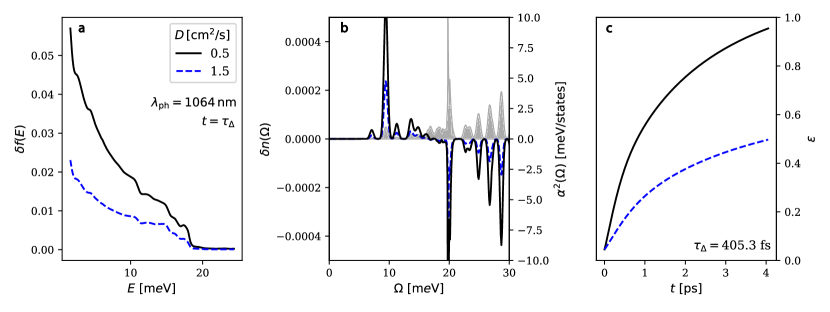
Figure 3: (a) Nonequilibrium excess quasiparticle $\delta\!f(E)$ and (b) excess phonon $\delta\!n(\Omega)$ distribution generated by the absorption of a photon with wavelength $\lambda_{\mathrm{ph}}=1064\,\mathrm{nm}$ at $t=\tau_{\Delta}$ for $\mathrm{NbN}$ with electronic diffusion coefficients of $D=1.5\,\mathrm{cm^{2}/s}$ and $D=0.5\,\mathrm{cm^{2}/s}$. (c) Quasiparticle-induced suppression parameter $\varepsilon(t)$. A value of $\varepsilon=0$ implies no suppression of $\Delta$.

Turning to the initial interactions of the optically excited quasiparticle, the lifetime of a quasiparticle of energy $\sim E_{\lambda}$ is extremely short relative to the timescale of variations of the superconducting order parameter $\tau_{\Delta}=\hbar/|\Delta|$ [39, 40]. Thus, the subsequent interactions are practically instantaneous from the perspective of $\Delta$. Initially, quasiparticle relaxation occurs primarily through electron-electron scattering and the emission of secondary electrons. These electrons quickly reach energies on the order of $\Omega_{\mathrm{D}}$, where relaxation via acoustic-phonon emission dominates [7, 40]. These emitted phonons possess short mean-free paths and contribute to pair-breaking. Hence, the initial distribution for Eqs. (1a) and (1b) is well approximated by a phonon-bubble initial condition [28]. These dynamics are illustrated in Fig. 1b.

To determine the phonon-bubble initial condition, we use Eq. (1b) and approximate the initial excess quasiparticle distribution $\delta\!f(E)=f(E)-f^{\mathrm{eq}}(E)$ as a delta function centered at $E_{\lambda}$, which gives that the initial phonon population is $n_{0}(\Omega)=\beta(E_{\lambda})\alpha^{2}(\Omega)$ [7], where the parameter $\beta(E_{\lambda})$ ensures that the initial energy of the phonon system is equal to the photon energy. $n_{0}(\Omega)$ and an equilibrium quasiparticle (Fermi-Dirac) distribution $f^{\mathrm{eq}}(E)$ characterize the phonon bubble. Eqs. (1a) and (1b) with the phonon-bubble initial condition then provide the subsequent quasiparticle and phonon dynamics that result from absorption of a photon.

In Fig. 3a and Fig. 3b, numerical solutions to Eqs. (1a) and (1b) for two different electronic diffusion coefficients $D$ are displayed. In these calculations, material parameters consistent with $\mathrm{NbN}$, and SNSPD geometries, were used [41], with $N(0)=15\,e\mathrm{V}^{-1}\mathrm{nm}^{-3}$, $N=50\,\mathrm{nm^{-3}}$, $|\Delta_{0}|\equiv|\Delta(I_{\rm{B}}=0,T=0)|=1.81\,\mathrm{m}e\mathrm{V}$, $T_{\mathrm{c}}=10\,\mathrm{K}$, and $d=5\,\mathrm{nm}$. $D=1.5\,\mathrm{cm^{2}/s}$ is typical of epitaxial $\mathrm{NbN}$ [41], while $D=0.5\,\mathrm{cm^{2}/s}$ is typical of polycrystalline $\mathrm{NbN}$ [28]. These material parameters can also be obtained ab initio from DFT rather than from experimental data [42, 3]. In our solutions, we found that for $0.5I_{\mathrm{dep}}\leq I_{\mathrm{B}}\leq 0.9I_{\mathrm{dep}}$, where $I_{\mathrm{dep}}$ is the depairing current, there was not a strong dependence of the generated quasiparticle population on $I_{\mathrm{B}}$. Hence, we set $I_{\mathrm{B}}=0.5I_{\mathrm{dep}}$, which incorporates the effect of smearing in $\rho(E)$ while also preserving the generality of the results to polycrystalline devices with switching currents on the order of $0.5I_{\mathrm{dep}}$. For smaller $D$, corresponding to greater disorder, $\alpha^{2}F(\Omega)$ is smeared; however, we do not expect this effect to have a significant impact on our results and thus we neglect it. In our solutions, we assume that the photon’s energy is initially distributed uniformly in a cylindrical volume of $V_{\mathrm{init}}=\pi\xi_{\rm{c}}^{2}d$ and $|\Delta(I_{\mathrm{B}},T)|$ is constant for the timescales of interest ($t\lesssim\tau_{\Delta}$). Further details regarding the numerical methods and validation are discussed in the Appendix and Supplemental Information.

By inserting $\delta\!f(E)$ into Eq. (2) we calculate the quasiparticle-induced suppression parameter

$$\varepsilon(t)=2\int_{|\Delta|}^{\infty}d\!E\,\frac{R(E,\Delta)}{|\Delta|}\delta\!f(E),$$ (3)

which characterizes the suppression of $|\Delta|$ and is displayed in Fig. 3c. The full Migdal-Eliashberg self-consistency equations on the real-frequency axis along with the strong-coupling Usadel equation could be used instead of the BCS self-consistency equation Eq. (2); however, the resulting complexity and effort to solve these equations would have been significant and beyond the scope of the current work. This approximation limits the quantitative accuracy of our model.

Fig. 3c illustrates that in dirtier materials with a smaller $D$, a larger nonequilibrium quasiparticle population is generated within $V_{\rm{init}}$, resulting in a more significant suppression of $|\Delta|$ in the initial stages following photon absorption. These results are consistent with the argument that a larger $D$ leads to more stringent requirements on the detector’s geometry to maintain photon sensitivity, e.g. reducing the film thickness and/or wire width [43].

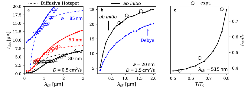
Figure 4: Comparison of the ab initio model (solid lines) against the phenomenological diffusive hotspot model [22, 31] (dashed lines) and experimental data (large open markers) [44, 45, 43]. (a) Determination of the detection current $I_{\mathrm{det}}$ for a given photon wavelength $\lambda_{\mathrm{ph}}$ and wire widths of $w=30\,\rm{nm},\,50\,\rm{nm},$ and $85\,\rm{nm}$ with $D=0.5\,\mathrm{cm^{2}/s}$ compared to the experimental data of Ref. [44]. A value of $\eta=0.2$ for the diffusive hotspot model gives the best fit (See Ref. [31] for a definition of $\eta$). (b) $I_{\mathrm{det}}$ as a function of $\lambda_{\mathrm{ph}}$ for $w=20\,\mathrm{nm}$ and parameters consistent with the material used in the experimental data of Ref. [43]. Results using both the full-bandwidth electron-phonon coupling (ab initio) and Debye models are displayed. (c) Ab initio predictions of $I_{\mathrm{det}}$ as a function of the reduced temperature $T/T_{\mathrm{c}}$ for $\lambda_{\mathrm{ph}}=515\,\rm{nm}$ compared to experimental data for the temperature-dependence of $\mathrm{NbTiN}$ from Ref. [45]. Since the data in this figure is not for $\mathrm{NbN}$, only qualitative agreement of the temperature dependence is expected. Calculations from the ab initio model are in arbitrary units.

We define the thermalization time of the quasiparticle and phonon system $\tau_{\mathrm{th}}$ by fitting the numerical solution for $\varepsilon(t)$ to an exponential $\varepsilon(t)=\varepsilon_{t\rightarrow\infty}(1-e^{-t/\tau_{\mathrm{th}}})$. For $\mathrm{NbN}$ at $T/T_{\rm{c}}=0.2$ with an electronic diffusion coefficient of $D=0.5\,\mathrm{cm^{2}/s}$ we find $\tau_{\mathrm{th}}=1.4\,\mathrm{ps}$ and for $D=1.5\,\mathrm{cm^{2}/s}$ we find $\tau_{\mathrm{th}}=1.8\,\mathrm{ps}$ for $\lambda_{\mathrm{ph}}=1064\,\mathrm{nm}$. That $\tau_{\mathrm{th}}>\tau_{\Delta}=405.3\,\mathrm{fs}$ is consistent with the results obtained by Vodolazov with the Debye model [28]; however, with the Debye model it is found that, for $D=0.5\,\mathrm{cm^{2}/s}$, $\tau_{\mathrm{th}}\approx 1.5\tau_{\Delta}$, whereas with the full-bandwidth electron-phonon coupling, we find $\tau_{\mathrm{th}}\approx 4\tau_{\Delta}$. The larger value of $\tau_{\mathrm{th}}$ obtained with the full-bandwidth electron-phonon coupling is in better agreement with experimental data [40]. We also note that $\tau_{\mathrm{th}}>\tau_{\Delta}$ implies that the local electron and phonon temperatures are still evolving when the region of suppressed superconductivity has diffused beyond $V_{\mathrm{init}}$. Hence, caution must be exercised when assuming there exists a well-defined electron and phonon temperature in $\mathrm{NbN}$ during the early stages of the quasiparticle cascade.

The microscopic treatment above is only suitable to account for the local suppression of superconductivity within $V_{\mathrm{init}}$ for $t\leq\tau_{\Delta}$. To determine if the suppression is sufficient to create a normal strip across the film, we must examine the dynamics of $\Delta$ across the full two-dimensional film and account for quantum fluctuations. These fluctuations are critical, as experimental and theoretical evidence suggests that detection in SNSPDs is assisted by vortex motion or phase-slippage [27]. In this picture, the suppression of superconductivity induced by the photon lowers the barrier for a $2\pi$-phase-slip of the superconducting order parameter. Several processes can lead to phase-slip events in nanowires, including (1) the passage of a single vortex across the wire; (2) a quantum or thermally activated phase-slip; or (3) a vortex/anti-vortex pair that unbinds due to the Magnus force from $I_{\mathrm{B}}$. We refer to these processes collectively as phase-slip events. Once a phase-slip event occurs, Joule heating due to the nonzero $I_{\mathrm{B}}$ can lead to thermal runaway, destroying superconductivity across the strip and resulting in a voltage spike corresponding to a detection event.

Phase-slip dynamics are naturally captured by the time-dependent Ginzburg-Landau (TDGL) equation

$$\frac{u}{\sqrt{1+\gamma^{2}|\psi|^{2}}} \left(\frac{\partial}{\partial t}+i\mu+\frac{1}{2}\gamma^{2}\frac{\partial|\psi|^{2}}{\partial t}\right)\psi=$$ (4)

$$\xi^{2}(\nabla-2ie\mathbf{A})^{2}\psi+(\alpha-|\psi|^{2})\psi,$$

where we have used dimensionless units with $u=\pi^{4}/14\zeta(3)=5.79$, $\gamma=10$, the normalized superconducting order parameter $\psi=\Delta/|\Delta_{0}|$, and the electric scalar potential $\mu(\mathbf{r},t)$ which satisfies a Poisson equation [46]. The parameter $\alpha(\mathbf{r},t)=(1-T/T_{\mathrm{c}}-\varepsilon(\mathbf{r},t))/(1-T/T_{\mathrm{c}})$ models the photon-induced suppression of $\psi$ at position $\mathbf{r}$ and time $t$ ($\alpha=1$ at equilibrium), where $\varepsilon(\mathbf{r},t)$ is calculated from the microscopic dynamics using Eq. (3). Here, we assume that the hotspot grows isotropically with a time-dependent radius $|\mathbf{r}(t)|=\sqrt{Dt}$. A more rigorous treatment of quasiparticle and phonon diffusion, along with solving Eqs. (1a) and (1b) self-consistently with Eq. (2), would significantly improve the accuracy for wires with larger $w$, which possess longer latency times between absorption and detection. The generalized TDGL equation with Usadel corrections for the supercurrent density $j_{\mathrm{S}}$ and $\Delta$ can also be used in place of Eq. (4) to improve validity at lower temperatures and large deviations from equilibrium [28]. However, as we will see shortly, the present model is sufficient to obtain reasonable quantitative accuracy.

We solve Eq. (4) with the Python package pyTDGL [47]. In these simulations, for each photon wavelength $\lambda_{\mathrm{ph}}$, we varied $I_{\mathrm{B}}$ while checking if the voltage arising from the formation of a normal strip across the wire exceeded a threshold and the phase difference across the terminals of the device exceeded $2\pi$. The current at which these criteria were met was determined to be the detection current $I_{\mathrm{det}}$. Note that since we perform the simulation over a coarse grid of bias currents, some quantization error is introduced. We restricted our simulation time to $t<15\,\mathrm{ps}$ for the wires with $w=30\,\rm{nm}$ and $w=50\,\rm{nm}$ and $t<25\,\mathrm{ps}$ for $w=85\,\rm{nm}$ to account for the longer latency between photon absorption and detection. For the epitaxial detector, where diffusion was much faster, with $w=20\,\rm{nm}$ the simulation time was restricted to $t<5\,\rm{ps}$. Further details on obtaining the numerical solutions to Eq. (4) are included in the Supplemental Information.

In Fig. 4, we show the resulting dependence of $I_{\mathrm{det}}$ on $\lambda_{\mathrm{ph}}$. We compare our calculations against the phenomenological diffusive normal-core model [22, 31] and experimental data from Ref. [44, 43]. We also compare the temperature dependence of $I_{\mathrm{det}}$ with the experimental data of Ref. [45]. However, the data of Ref. [45] is for $\mathrm{NbTiN}$ and should only be checked for qualitative agreement. In our calculations, we assumed $D=0.5\,\mathrm{cm^{2}/s}$ for the polycrystalline detectors in Ref. [44] and $D=1.5\,\mathrm{cm^{2}/s}$ for the epitaxial detector of Ref. [43]. In both cases, we set $\tau_{\mathrm{esc}}=10\,\mathrm{ps}$. We observe that the qualitative behavior of the ab initio model is similar to the experimental data and there is reasonable quantitative agreement with the results of Ref. [43] and [44]. In Fig. 4b, it can also be seen that the predictions of the ab initio model improve significantly over the predictions of the Debye model. We emphasize that our model achieves this improved quantitative agreement without the use of any free parameters, which affirms the merit of our approach. We thus propose that the methods here can be used to design the next generation of SNSPDs, exploring new materials and geometries to extend the wavelength sensitivity and other device metrics to new regimes.

We anticipate incorporating thermal equations for the electron and phonon temperatures and a circuit model to account for Joule heating, the kinetic inductance of the film, and the external circuitry will further improve the quantitative accuracy. These additional equations are most relevant in the presence of a small shunt resistance or small $I_{\mathrm{B}}$, where these processes may play a role in the initial phase slip and in initiating a state of thermal runaway, such as at shorter $\lambda_{\mathrm{ph}}$ for $w=$30\text{\,}\mathrm{nm}$$ and $D=0.5\,\mathrm{cm^{2}/s}$ as in Fig. 4a. Thermal fluctuations can also be incorporated into Eq. (4) to allow for the determination of the internal detection efficiency below $I_{\mathrm{det}}$ and the prediction of dark count rates [48, 49]. Finally, the optical absorption efficiency can also be calculated [50] and integrated with our model. It would then be possible to construct an end-to-end model going from the crystal structure of a material to its system detection efficiency, consisting of the product of the optical absorption efficiency and internal detection efficiency calculated by our model, and the resulting voltage spike and macroscopic dynamics by incorporating a circuit model [29].

In summary, we have demonstrated a framework for modeling the performance of superconducting devices ab initio. To illustrate the effectiveness of our approach, we apply our model to describe superconducting nanowire single-photon detectors, with $\mathrm{NbN}$ as the material platform of choice due to its relevance as a material for superconducting devices. However, the methods discussed here can easily be extended to other devices and materials. With the existing difficulties in the fabrication and engineering of superconductors with novel structures or difficult materials, these methods can inform the future direction for designing superconducting devices for enhanced performance.

I acknowledgements

The authors thank Rohit Prasankumar and Jason Allmaras for their helpful discussions. This work was funded in part by the Defense Sciences Office (DSO) of the Defense Advanced Research Projects Agency (DARPA). AS acknowledges support from the NSF GRFP, RF acknowledges support from the Alan McWhorter fellowship, and EB acknowledges support from the NSF GRFP. MS and CH acknowledge support from Intellectual Ventures Property Holdings and usage of computational resources of the dCluster of the Graz University of Technology.

II Appendix

II.1 Numerical solutions to the kinetic equations

The kernel functions in Eqs. (1a) and (1b) of the main text are given by

$$K_{ph-\mathrm{e}}(E,\Omega) =\left(1-\frac{\Delta^{2}}{E(E+\Omega)}\right)\{f(E)[1-f(E+\Omega)]n(\Omega)-f(E+\Omega)[1-f(E)][n(\Omega)+1]\}$$ (5a)

$$K_{e-\mathrm{ph}}(E,\Omega) =\left(1-\frac{\Delta^{2}}{E(E-\Omega)}\right)\{f(E)[1-f(E-\Omega)][n(\Omega)+1]-[1-f(E)]f(E-\Omega)n(\Omega)\}$$ (5b)

$$K_{\mathrm{R}}(E,\Omega)=\left(1+\frac{\Delta^{2}}{E(\Omega-E)}\right)\{f(E)f(\Omega-E)[n(\Omega)+1]-[1-f(E)][1-f(\Omega-E)]n(\Omega)\}$$ (5c)

$$K_{\mathrm{S}}(E,E^{\prime},\Omega)=\left(1-\frac{\Delta^{2}}{EE^{\prime}}\right)\{f(E)[1-f(E^{\prime})]n(\Omega)-f(E^{\prime})[1-f(E)][n(\Omega)+1]\}$$ (5d)

$$K_{\mathrm{B}}(E,E^{\prime},\Omega)=\frac{1}{2}\left(1+\frac{\Delta^{2}}{EE^{\prime}}\right)\{[1-f(E)][1-f(E^{\prime})]n(\Omega)-f(E)f(E^{\prime})[n(\Omega)+1]\}.$$ (5e)

Numerical solutions to Eq. (1a), (1b), (5a-e) were obtained with a forward Euler scheme, where the integrals were evaluated numerically at each timestep. For each timestep, it was checked that energy was conserved within 0.1% of the starting energy for $t\leq\tau_{\Delta}$ when $\tau_{\mathrm{esc}}=\infty$. In most of our simulations, this error criteria was often exceeded by orders of magnitude. Further details and examples of the time evolution of $\delta\!f(E)$ and $\delta\!n(\Omega)$ are included in the Supplemental Information. Details of the mesh sizes and inputs used in pyTDGL can also be found in the Supplemental Information.

II.2 Quasiparticle density of states

The normalized quasiparticle density of states for a superconducting film in the dirty limit is given by $\rho(E)=\mathrm{Re}\{\cos\Theta(E)\}$, where $\Theta(E)$ can be obtained from the Usadel equation on the imaginary-frequency axis

$$\hbar D\nabla^{2}\Theta(\vec{\mathbf{r}},i\omega_{n})+2|\Delta(\vec{\mathbf{r}})|\cos\Theta(\vec{\mathbf{r}},i\omega_{n})$$ (6)

$$-\left(2\hbar\omega_{n}+\frac{D}{\hbar}q^{2}\cos\Theta(\vec{\mathbf{r}},i\omega_{n})\right)\sin\Theta(\vec{\mathbf{r}},i\omega_{n})=0$$

and performing an analytical continuation to the real-frequency axis $i\omega_{n}\rightarrow E+i0^{+}$. For a uniform film, the spatial dependence of $\Theta$ and $|\Delta|$ can be ignored, there are no boundary conditions, and the diffusive term $\hbar D\nabla^{2}\Theta(\vec{\mathbf{r}},i\omega_{n})$ is zero. The order parameter $|\Delta|$ satisfies the BCS self-consistency equation

$$|\Delta|\ln\left(\frac{T}{T_{{\rm c}}}\right)+2\pi k_{\mathrm{B}}T\sum_{\omega_{n}\geq 0}\left(\frac{|\Delta|}{\hbar\omega_{n}}-\sin\Theta(i\omega_{n})\right)=0,$$ (7)

where $k_{\mathrm{B}}$ is the Boltzmann constant, $T_{\mathrm{c}}$ is the critical temperature, $\omega_{n}=\pi T(2n+1)k_{\rm{B}}/\hbar$ is the $n$-th Matsubara frequency, and $\Theta(i\omega_{n})$ is the pairing-angle parametrization of the Nambu-Gor’kov Green’s function [51, 52]. The superfluid momentum $q$ is related to the supercurrent density via

$$j_{\mathrm{S}}=\frac{I_{\mathrm{B}}}{wd} =\frac{2\pi k_{\mathrm{B}}T}{|e|}\sigma_{0}q\sum_{n=0}^{\infty}\sin^{2}\Theta(i\omega_{n}),$$ (8)

where $\sigma_{0}=1/\rho_{\mathrm{N}}$ is the Drude conductivity. We define the spectral function

$$R(E,\Delta)=\mathrm{Im}\{\sin\Theta(E)\}$$ (9)

from the main text.

Equations 6 and 7 are solved simultaneously with a left-preconditioned Newton-Krylov method [53]. The preconditioner is constructed from the Jacobian of equations 6 and 7 assuming a BCS ($q=0$) solution. The infinite Matsubara sum in equation 7 is approximated with a quadrature rule for sums [54].

II.3 Density Functional Theory calculations

We employed the Quantum Espresso code [55] to compute the structural, electronic, and harmonic phonon properties of bulk NbN using first-principles DFPT. The exchange-correlation functional was described by the Perdew-Burke-Ernzerhof (PBE) [56] version of the generalized gradient approximation (GGA) in combination with optimized norm-conserving Vanderbilt pseudopotentials [57, 58]. The convergence threshold for the self-consistent field was set to $10^{-10}$ Ry for the energy difference between consecutive electronic steps and structural relaxations were performed until the forces on each atom were less than $10^{-6}$ Ry/Å. A plane-wave kinetic energy cutoff of 80 Ry was used, along with an $18\times 18\times 18$ k-point grid and a Methfessel-Paxton smearing [59] of 0.3 Ry to sample the Brillouin zone for self-consistent calculations. Such a large electronic smearing is needed to avoid imaginary frequencies in the harmonic DFPT calculation of phonon properties, as disorder, impurities, and anharmonic effects are not accounted for. As can be appreciated in Fig. 2, the calculated phonon dispersion compares well to experimental data [37].

For phonon calculations, we employed a $6\times 6\times 6$ q-point grid and a threshold of self-consistency of $10^{-14}$ Ry to obtain the dynamical matrices within the harmonic approximation. To interpolate the electronic and phononic properties onto finer grids, we utilized the Electron-Phonon Wannier (EPW) code [33] using Nb $s,p,d$ and N $p$ orbitals as starting projections for the Wannierization. Specifically, interpolation to fine grids of $30\times 30\times 30$ for both electrons and phonons was performed to obtain isotropic Eliashberg spectral functions $\alpha^{2}F(\Omega)$.

References

- Eliashberg [1960] G. Eliashberg, Sov. Phys. JETP 11, 696 (1960).
- Allen and Dynes [1975] P. B. Allen and R. C. Dynes, Phys. Rev. B 12, 905 (1975).
- Pellegrini and Sanna [2024] C. Pellegrini and A. Sanna, Nature Reviews Physics 6, 509 (2024).
- Prange [1964] R. E. Prange, Physical Review 134, A566 (1964).
- Eliashberg [1970] G. M. Eliashberg, JETP Lett. (USSR) (Engl. Transl.); (United States) 11 (1970).
- Eliashberg [1972] G. Eliashberg, Sov Phys JETP 34, 668 (1972).
- Chang and Scalapino [1977] J.-J. Chang and D. J. Scalapino, Physical Review B 15, 2651 (1977).
- Ashby and Rickayzen [1981] J. V. Ashby and G. Rickayzen, Journal of Physics F: Metal Physics 11, 2595 (1981).
- Goldie and Withington [2012] D. Goldie and S. Withington, Superconductor Science and Technology 26, 015004 (2012).
- Marsili et al. [2013] F. Marsili, V. B. Verma, J. A. Stern, S. Harrington, A. E. Lita, T. Gerrits, I. Vayshenker, B. Baek, M. D. Shaw, R. P. Mirin, and S. W. Nam, Nature Photonics 7, 210 (2013), publisher: Nature Publishing Group.
- Reddy et al. [2020] D. V. Reddy, R. R. Nerem, S. W. Nam, R. P. Mirin, and V. B. Verma, Optica 7, 1649 (2020), publisher: Optica Publishing Group.
- Chang et al. [2021] J. Chang, J. W. N. Los, J. O. Tenorio-Pearl, N. Noordzij, R. Gourgues, A. Guardiani, J. R. Zichi, S. F. Pereira, H. P. Urbach, V. Zwiller, S. N. Dorenbos, and I. Esmaeil Zadeh, APL Photonics 6, 036114 (2021).
- Verma et al. [2021] V. B. Verma, B. Korzh, A. B. Walter, A. E. Lita, R. M. Briggs, M. Colangelo, Y. Zhai, E. E. Wollman, A. D. Beyer, J. P. Allmaras, H. Vora, D. Zhu, E. Schmidt, A. G. Kozorezov, K. K. Berggren, R. P. Mirin, S. W. Nam, and M. D. Shaw, APL Photonics 6, 056101 (2021).
- Taylor et al. [2023] G. G. Taylor, A. B. Walter, B. Korzh, B. Bumble, S. R. Patel, J. P. Allmaras, A. D. Beyer, R. O’Brient, M. D. Shaw, and E. E. Wollman, Optica 10, 1672 (2023).
- Hochberg et al. [2019] Y. Hochberg, I. Charaev, S.-W. Nam, V. Verma, M. Colangelo, and K. K. Berggren, Phys. Rev. Lett. 123, 151802 (2019).
- Hochberg [2022] Y. Hochberg, Physical Review D 106, 10.1103/PhysRevD.106.112005 (2022).
- Korzh et al. [2020] B. Korzh, Q.-Y. Zhao, J. P. Allmaras, S. Frasca, T. M. Autry, E. A. Bersin, A. D. Beyer, R. M. Briggs, B. Bumble, M. Colangelo, G. M. Crouch, A. E. Dane, T. Gerrits, A. E. Lita, F. Marsili, G. Moody, C. Peña, E. Ramirez, J. D. Rezac, N. Sinclair, M. J. Stevens, A. E. Velasco, V. B. Verma, E. E. Wollman, S. Xie, D. Zhu, P. D. Hale, M. Spiropulu, K. L. Silverman, R. P. Mirin, S. W. Nam, A. G. Kozorezov, M. D. Shaw, and K. K. Berggren, Nature Photonics 14, 250 (2020), publisher: Nature Publishing Group.
- Charaev et al. [2024] I. Charaev, E. K. Batson, S. Cherednichenko, K. Reidy, V. Drakinskiy, Y. Yu, S. Lara-Avila, J. D. Thomsen, M. Colangelo, F. Incalza, K. Ilin, A. Schilling, and K. K. Berggren, Nature Communications 15, 3973 (2024), publisher: Nature Publishing Group.
- Cherednichenko et al. [2021] S. Cherednichenko, N. Acharya, E. Novoselov, and V. Drakinskiy, Superconductor Science and Technology 34, 044001 (2021), publisher: IOP Publishing.
- Arpaia [2017] R. Arpaia, Physical Review B 96, 10.1103/PhysRevB.96.064525 (2017).
- Charaev et al. [2023] I. Charaev, D. A. Bandurin, A. T. Bollinger, I. Y. Phinney, I. Drozdov, M. Colangelo, B. A. Butters, T. Taniguchi, K. Watanabe, X. He, O. Medeiros, I. Božović, P. Jarillo-Herrero, and K. K. Berggren, Nature Nanotechnology 18, 343 (2023), publisher: Nature Publishing Group.
- Semenov et al. [2001] A. D. Semenov, G. N. Gol’tsman, and A. A. Korneev, Physica C: Superconductivity 351, 349 (2001).
- Semenov et al. [1995] A. D. Semenov, R. S. Nebosis, Y. P. Gousev, M. A. Heusinger, and K. F. Renk, Phys. Rev. B 52, 581 (1995).
- Yang et al. [2007] J. K. W. Yang, A. J. Kerman, E. A. Dauler, V. Anant, K. M. Rosfjord, and K. K. Berggren, IEEE Transactions on Applied Superconductivity 17, 581 (2007).
- Kozorezov et al. [2007] A. G. Kozorezov, J. K. Wigmore, D. Martin, P. Verhoeve, and A. Peacock, Phys. Rev. B 75, 094513 (2007).
- Kozorezov et al. [2000] A. G. Kozorezov, A. F. Volkov, J. K. Wigmore, A. Peacock, A. Poelaert, and R. den Hartog, Phys. Rev. B 61, 11807 (2000).
- Engel et al. [2015] A. Engel, J. J. Renema, K. Il’in, and A. Semenov, Superconductor Science and Technology 28, 114003 (2015).
- Vodolazov [2017] D. Vodolazov, Physical Review Applied 7, 10.1103/PhysRevApplied.7.034014 (2017).
- Berggren et al. [2018] K. K. Berggren, Q.-Y. Zhao, N. Abebe, M. Chen, P. Ravindran, A. McCaughan, and J. C. Bardin, Superconductor Science and Technology 31, 055010 (2018).
- Allmaras [2020] J. P. Allmaras, Modeling and development of superconducting nanowire single-photon detectors (California Institute of Technology, 2020).
- Semenov [2021] A. D. Semenov, Superconductor Science and Technology 34, 054002 (2021).
- Lucrezi et al. [2024] R. Lucrezi, P. P. Ferreira, S. Hajinazar, H. Mori, H. Paudyal, E. R. Margine, and C. Heil, Communications Physics 7, 33 (2024).
- Lee et al. [2023] H. Lee, S. Poncé, K. Bushick, S. Hajinazar, J. Lafuente-Bartolome, J. Leveillee, C. Lian, J.-M. Lihm, F. Macheda, H. Mori, et al., npj Computational Materials 9, 156 (2023).
- Budoyo et al. [2016] R. Budoyo, J. B. Hertzberg, C. Ballard, K. Voigt, Z. Kim, J. Anderson, C. Lobb, and F. Wellstood, Physical Review B 93, 024514 (2016).
- Liu et al. [2024] C. H. Liu, D. C. Harrison, S. Patel, C. D. Wilen, O. Rafferty, A. Shearrow, A. Ballard, V. Iaia, J. Ku, B. L. T. Plourde, and R. McDermott, Phys. Rev. Lett. 132, 017001 (2024).
- Benevides et al. [2024] R. Benevides, M. Drimmer, G. Bisson, F. Adinolfi, U. v. Lüpke, H. M. Doeleman, G. Catelani, and Y. Chu, Phys. Rev. Lett. 133, 060602 (2024).
- Christensen et al. [1979] A. Christensen, O. Dietrich, W. Kress, W. Teuchert, and R. Currat, Solid State Communications 31, 795 (1979).
- Ferreira et al. [2024] P. Ferreira, R. Lucrezi, I. Guilhon, M. Marques, L. Teles, C. Heil, and L. Eleno, Materials Today Physics 48, 101547 (2024).
- Kaplan et al. [1976] S. B. Kaplan, C. Chi, D. Langenberg, J.-J. Chang, S. Jafarey, and D. Scalapino, Physical Review B 14, 4854 (1976).
- Il’in et al. [1998] K. S. Il’in, I. I. Milostnaya, A. A. Verevkin, G. N. Gol’tsman, E. M. Gershenzon, and R. Sobolewski, Applied Physics Letters 73, 3938 (1998), https://pubs.aip.org/aip/apl/article-pdf/73/26/3938/18538627/3938_1_online.pdf .
- Chockalingam et al. [2008] S. P. Chockalingam, M. Chand, J. Jesudasan, V. Tripathi, and P. Raychaudhuri, Phys. Rev. B 77, 214503 (2008).
- Giustino [2014] F. Giustino, Materials modelling using density functional theory: properties and predictions (Oxford University Press, 2014).
- Cheng et al. [2020] R. Cheng, J. Wright, H. G. Xing, D. Jena, and H. X. Tang, Applied Physics Letters 117, 132601 (2020), https://pubs.aip.org/aip/apl/article-pdf/doi/10.1063/5.0018818/14539879/132601_1_online.pdf .
- Marsili et al. [2012] F. Marsili, F. Bellei, F. Najafi, A. E. Dane, E. A. Dauler, R. J. Molnar, and K. K. Berggren, Nano letters 12, 4799 (2012).
- Gourgues et al. [2019] R. Gourgues, J. W. N. Los, J. Zichi, J. Chang, N. Kalhor, G. Bulgarini, S. N. Dorenbos, V. Zwiller, and I. E. Zadeh, Opt. Express 27, 24601 (2019).
- Kramer and Watts-Tobin [1978] L. Kramer and R. J. Watts-Tobin, Phys. Rev. Lett. 40, 1041 (1978).
- Bishop-Van Horn [2023] L. Bishop-Van Horn, Comput. Phys. Commun. 291, 108799 (2023).
- Salvoni et al. [2022] D. Salvoni, M. Ejrnaes, A. Gaggero, F. Mattioli, F. Martini, H. Ahmad, L. Di Palma, R. Satariano, X. Yang, L. You, F. Tafuri, G. Pepe, D. Massarotti, D. Montemurro, and L. Parlato, Phys. Rev. Appl. 18, 014006 (2022).
- Bartolf et al. [2010] H. Bartolf, A. Engel, A. Schilling, K. Il’in, M. Siegel, H.-W. Hübers, and A. Semenov, Phys. Rev. B 81, 024502 (2010).
- Sunter and Berggren [2018] K. A. Sunter and K. K. Berggren, Appl. Opt. 57, 4872 (2018).
- Usadel [1970] K. D. Usadel, Physical Review Letters 25, 507 (1970).
- Rammer [1987] J. Rammer, Phys. Rev. B 36, 5665 (1987).
- [53] D. A. Knoll and D. E. Keyes, Journal of Computational Physics 193, 357.
- [54] H. Monien, Explicit Methods in Number Theory 12, 1809.
- Giannozzi et al. [2017] P. Giannozzi, O. Andreussi, T. Brumme, O. Bunau, M. B. Nardelli, M. Calandra, R. Car, C. Cavazzoni, D. Ceresoli, M. Cococcioni, et al., Journal of physics: Condensed matter 29, 465901 (2017).
- Perdew et al. [1996] J. P. Perdew, K. Burke, and M. Ernzerhof, Physical review letters 77, 3865 (1996).
- Schlipf and Gygi [2015] M. Schlipf and F. Gygi, Computer Physics Communications 196, 36 (2015).
- Hamann [2013] D. Hamann, Physical Review B—Condensed Matter and Materials Physics 88, 085117 (2013).
- Methfessel and Paxton [1989] M. Methfessel and A. Paxton, physical review B 40, 3616 (1989).