Fast Iterative and Task-Specific Imputation with Online Learning

Abstract

Missing feature values are a significant hurdle for downstream machine-learning tasks such as classification and regression. However, they are pervasive in multiple real-life use cases, for instance, in drug discovery research. Moreover, imputation methods might be time-consuming and offer few guarantees on the imputation quality, especially for not-missing-at-random mechanisms. We propose an imputation approach named F3I based on the iterative improvement of a K-nearest neighbor imputation that learns the weights for each neighbor of a data point, optimizing for the most likely distribution of points over data points. This algorithm can also be jointly trained with a downstream task on the imputed values. We provide a theoretical analysis of the imputation quality by F3I for several types of missing mechanisms. We also demonstrate the performance of F3I on both synthetic data sets and real-life drug repurposing and handwritten-digit recognition data.

1 Introduction

Most machine-learning approaches assume full access to the features of the input data points. However, missing values might arise due to the incompleteness of public databases or measurement errors. Research on the imputation of missing values and inference on possibly missing data is motivated by the fact that naive approaches would not fare well. Indeed, ignoring samples with missing values might lead to severe data loss and meaningless downstream models, for classification or regression. On the other hand, replacing missing values with zeroes (or any “simple” univariate approach such as taking the mean or the median) can considerably distort the distribution of data values, as there is a more significant weight on the default value for missing entries, and then perhaps bias the training of a downstream model for classification or regression tasks. However, multivariate approaches are often time-consuming and prohibitive for high-dimensional data sets, as in biology and medicine.

The literature often distinguishes three main categories of missingness mechanisms (Rubin, 1976) depending on the relationship between the probability $p^{\text{miss}}$ of a missing value and the data. The simplest one is Missing-Completely-At-Random (MCAR), where that probability is independent of the data. This can be applied when the measurement tools fail at some probability regardless of the analyzed data. The second, more complex, setting is Missing-At-Random (MAR), where $p^{\text{miss}}$ only depends on the observed (not missing) data. An example of MAR is when male patients drop out more often from a clinical study than female patients. Finally, the Missing-Not-At-Random setting (MNAR), where $p^{\text{miss}}$ depends on both the observed and missing data, is widely regarded as the most challenging setting for analysis because the actual values might not be identifiable.

2 Related Work

As previously mentioned, the fastest approaches to imputation are often univariate because they are simple operations applied feature-wise to a data set. For instance, the missing value for a feature corresponding to a column of the data matrix might be replaced by the mean or the median of all non-missing values or even by zeroes in that column. Yet, such naive approaches might severely distort the distribution of values (Le Morvan & Varoquaux, 2024). That fact opened the path to multiple multivariate methods, such as MICE (van Buuren & Groothuis-Oudshoorn, 2011), MissForest (Stekhoven & Bühlmann, 2012), MIDAS (Seu et al., 2022), Optimal Transport-based algorithms (Muzellec et al., 2020), matrix factorizations (Mazumder et al., 2010), penalized logistic regression methods (van Loon et al., 2024), Bayesian network-based approaches (for instance, MIWAE (Mattei & Frellsen, 2019) for MAR mechanisms, and its MNAR counterpart not-MIWAE (Ipsen et al., 2021)) and K-nearest-neighbor (KNN) imputations (Troyanskaya et al., 2001). Some recent works also provide a pipeline for the automated finetuning and refinement of imputers, such as MIRACLE (Kyono et al., 2021) or HyperImpute (Jarrett et al., 2022). Among all of those methods, MissForest (Stekhoven & Bühlmann, 2012) and sometimes KNN imputation are often reported as the best-performing approaches imputation-wise (Emmanuel et al., 2021; Joel et al., 2024). However, as the number of features increases, so does the computation time, making most of those approaches untractable on practical data sets, for instance, in biology, where the feature set might represent genes that are approximately $20,000$ in humans.

Methods developed for multivariate time-series data might also be adapted to single-timepoint data sets, for instance, Conditional Score-based Diffusion Models (CDSI) (Tashiro et al., 2021), methods using Generative Adversarial Networks (Luo et al., 2018; Yoon et al., 2018) or Last Observation Carried Forward (LOCF), where the last non-missing value is duplicated until the next non-missing time point. However, we restrict our study to single-timepoint data.

Moreover, many published imputation methods come without any guarantee on the quality of the imputation or often on the more straightforward settings such as MCAR (Mazumder et al., 2010) and MAR (Śmieja et al., 2018); with a few exceptions such as (Tang et al., 2003; Mohan et al., 2018; Sportisse et al., 2020) for pure imputation tasks, and NeuMiss networks (Le Morvan et al., 2020), which tackle a classification task in the presence of missing values. However, the MCAR and MAR settings are usually not applicable to real-life data, and (Tang et al., 2003; Mohan et al., 2018; Sportisse et al., 2020) rely on an assumption of data generation through low-rank or linear random models instead of simpler data distributions.

Notwithstanding, nearest-neighbor imputers are known to be performant in practice and relatively fast (Seu et al., 2022; Joel et al., 2024), at the price of some distortion in high-dimensional data sets (Beretta & Santaniello, 2016). This observation led us to consider an improvement of a nearest-neighbor imputation that preserves the data distribution even in larger dimensions while remaining computationally fast.

Algorithm 1 Imputation improvement model Impute$(\cdot;\bm{\alpha},Z)$

 Input: Guess for a sample $\bm{x}\in\mathbb{R}^{F}$, missing indicator for that sample $\bm{m}\in\{0,1\}^{F}$

 Parameters: Number of neighbors $K$, weights $\bm{\alpha}\in\triangle_{K}$, reference set $Z=\{\bm{z}^{0},\bm{z}^{1},\dots,\bm{z}^{N^{\prime}}\}\subset\mathbb{R}^{F}$, $N^{\prime}\geq K$

 Output: Improved guess $\widetilde{\bm{x}}\in\mathbb{R}^{F}$

 # Neighbor indices by increasing Chebychev distance

 # $\overset{1,2,\dots,K}{\arg\,\min}_{j\leq N}$ selects the $K$ elements in $1,2,\dots,N$

 # with smallest values (with a k-d tree for instance)

 $(n_{1},n_{2},\dots,n_{K})\leftarrow\overset{1,2,\dots,K}{\arg\,\min}_{j\leq N}\max_{f\leq F}|x_{f}-z^{j}_{f}|$

 $\widetilde{x}_{f}\leftarrow\sum_{k\leq K}\alpha_{k}z^{n_{k}}_{f}$ for any $f\leq F$, $m^{f}=1$

2.1 Contributions

In Section 3, we describe a simple algorithm named Fast Iterative Improvement for Imputation (F3I) based on the automatically guided improvement of a nearest-neighbor imputer. F3I combines two ingredients: a novel objective function for preserving data distribution during imputation and a fast routine to optimize that function by drawing a parallel with the problem of expert advice in online learning (Cesa-Bianchi & Lugosi, 2006; De Rooij et al., 2014; Lattimore & Szepesvári, 2020). This algorithm theoretically guarantees imputation quality in some MCAR, MAR, and MNAR settings, listed in Section 4. Furthermore, as described in Section 5, this imputation can also be combined with a downstream task to increase the performance, as noted by other authors, both empirically (Le Morvan et al., 2021; Le Morvan & Varoquaux, 2024; Vo et al., 2024) and on a theoretical level (Le Morvan et al., 2021; Ayme et al., 2023, 2024). Finally, we illustrate the performance of F3I compared to other baselines on synthetic and real-life data sets for drug repurposing and handwritten-digit recognition in Section 6.

2.2 Notation

In the remainder of the paper, we denote $v$ a scalar, $\bm{v}$ a vector and $V$ a matrix. $\bm{v}^{i}$ is the $i^{th}$ column and $\bm{v}_{j}$ is the $j^{th}$ row of matrix $V$, and $v^{j}_{i}$ is the coefficient at position $(i,j)$ in $V$ for $i,j>0$. For any $K\geq 2$, $\triangle_{K}\triangleq\{\bm{p}\in[0,1]^{K}\mid\sum_{k\leq K}p_{k}=1\}$ is the simplex of dimension $K$. Finally, we denote the initial data matrix with missing values $X\in(\mathbb{R}\cup\{\texttt{NaN}\})^{N\times F}$, where $N$ is the number of samples and $F$ the number of features, and $X^{\star}\in\mathbb{R}^{N\times F}$ the full (unavailable) data matrix. Finally, we introduce $m^{f}_{i}\in\{0,1\}$, the random variable that indicates whether the value at position $(i,f)$ is missing in the input data matrix, where $m^{f}_{i}=1$ means it is missing.

3 Fast Iterative Improvement for Imputation

The key idea is that we would like to replace missing values in $X$ with the corresponding most probable real numbers by iteratively applying a “good” combination of values in the data set, starting from a simple guess obtained through K-nearest neighbor imputation. For each value $x^{f}_{i}$, we are looking to fit the weights $\bm{\alpha}=(\alpha_{1},\alpha_{2},\dots,\alpha_{K})$ of a convex combination of the $K$ closest neighbors of $\bm{x}_{i}$ in some reference set $Z\in\mathbb{R}^{N^{\prime}\times F}$ $\bm{z}_{i(1)},\bm{z}_{i(2)},\dots,\bm{z}_{i(K)}$. The neighbors are ordered by their increasing Chebychev distance to $\bm{x}_{i}$, which is empirically less noisy than the Euclidean distance. We denote that imputation improvement model $\texttt{Impute}(\bm{x}_{i};\bm{\alpha},Z)$, which is fully described in Algorithm 1. When the reference set is obvious, we define $\bm{x}(\bm{\alpha})\triangleq\texttt{Impute}(\bm{x};\bm{\alpha},Z)$.

3.1 Theoretical Assumptions

In this section, we state assumptions about the data generation procedure to derive theoretical guarantees from our algorithm. In practice, the algorithm can also be applied to real-life data, as we will demonstrate in our empirical study. First, we assume that each value in the full data matrix is drawn iid from a fixed-variance Gaussian distribution.

Assumption 3.1.

One dimensional-Gaussian data distributions. There exist $\bm{\mu}\in\mathbb{R}^{F}$ and $\sigma>0$ such that, for any sample $i\leq N$ and any feature $f\leq F$, $(x^{\star})^{f}_{i}\sim_{\text{iid}}\mathcal{N}(\mu_{f},\sigma^{2})\;.$

The random indicator variables $m^{f}_{i}$ are then independently drawn according to the missingness mechanism with probability $p^{\text{miss}}$. If $m^{f}_{i}=1$, then the coefficient at position $(i,f)$ $x^{f}_{i}$ in $X$ is unavailable, otherwise, $x^{f}_{i}=(x^{\star})^{f}_{i}$. We will provide an analysis of our algorithm for three types of missingness mechanisms.

Assumption 3.2.

MCAR mechanism: Bernouilli distribution. The random indicator variables for missing values $m^{f}_{i}$ are drawn iid from $\mathcal{B}(p^{\text{miss}}(\bm{x}))$, where $p^{\text{miss}}(\bm{x})\in(0,1)$ is a constant value for any $\bm{x}$.

Assumption 3.3.

MAR mechanism. We assume a subset $\mathcal{F}_{o}$ of size $F_{o}<F$ features is always observed. We denote $(x^{\star})^{\text{$\mid$ obs}}_{i}\triangleq(x^{\star}_{i}[f])_{f\in\mathcal{F}_{o}}$. Then there exist a function $p^{\text{miss}}$, $\forall\bm{x}\in\mathbb{R}^{F_{o}}$, $\mathbb{P}(m^{f}_{i}=1\mid(x^{\star})^{\text{$\mid$ obs}}_{i}=\bm{x})=p^{\text{miss}}(\bm{x})\;.$

Assumption 3.4.

MNAR mechanism: Gaussian self-masking (Assumption $4$ from Le Morvan et al. (2020)). The probability of event $\{m^{f}_{i}=1\}$ depends on $(x^{\star})^{f}_{i}$: $\exists K_{f}\in(0,1),\ \forall x\in\mathbb{R}$, $\mathbb{P}(m^{f}_{i}=1\mid(x^{\star})^{f}_{i}=x)=K_{f}e^{-\frac{1}{\sigma^{2}}(x-\mu_{f})^{2}}=p^{\text{miss}}(\bm{x})\;.$

The full data generation procedure is formally described in Algorithm 3 in the Appendix. We denote the corresponding distribution of points $\mathcal{D}\triangleq\mathcal{N}(\bm{\mu},\sigma^{2}\text{I}_{d})\otimes p^{\text{miss}}$, where the missingness mechanism is applied to points drawn from $\mathcal{N}(\bm{\mu},\sigma^{2}\text{I}_{d})$. We also want to ensure that there are exactly $K$ neighbors for the initial simple guesses and that we know a (constant) upper bound on the norm of any feature vectors.

Assumption 3.5.

Number of neighbors $K$. In the remainder of the paper, if $\{i\leq N\mid m^{f}_{i}=0\}$ is the set of data point indices for which the feature $f$ is not missing, then $K\leq\min_{f\leq F}|\{i\leq N\mid m^{f}_{i}=0\}|$. Without a loss of generality, $\min_{f\leq F}|\{i\leq N\mid m^{f}_{i}=0\}|\geq 2$ (otherwise, we can ignore the corresponding feature).

Assumption 3.6.

Upper bound on any of the $(\|\bm{x}_{i}\|^{2}_{2})_{i\leq n}$. We assume a constant $S>0$ exists, such that for any $i\leq N$, $\|\bm{x}_{i}\|^{2}_{2}\leq S$ (ignoring potential missing values). Up to renormalization, we assume that $S=1$. Moreover, the initial imputation step (the “simple guess”) preserves that condition, meaning that for any $i\leq N$ and $t\geq 0$, $\|\bm{x}^{t}_{i}\|^{2}_{2}\leq S$, where $X^{0}$ is the imputed data matrix with the initial imputation step, and $X^{t}$ for $t\geq 1$ is obtained through Algorithm 1.

Remark 3.7.

Assumption 3.6 can hold. Indeed, Assumption 3.6 is satisfied by the K-nearest neighbor imputation with uniform weights, where the imputed value equals the mean of all feature-wise values from the $K$ neighbors.

The goal of our algorithm F3I is to determine the proper weights in a nearest-neighbor imputation in a data-driven way that preserves the data distribution. But how do we define that property?

3.2 Objective Function For Imputing Missing Values

Ideally, if we had access to the true distribution on feature vectors (according to Assumption 3.1, to $\bm{\mu}$ and $\sigma$), we would like to set the weights $\bm{\alpha}\in\triangle_{K}$, the simplex of dimension $K$, such that the following quantity is maximized

$$\mathbb{E}_{\bm{x}\sim\mathcal{D}}\left[\mathds{1}(\Phi_{\bm{\mu},\sigma}(\texttt{Impute}\big{(}\bm{x}^{0};\bm{\alpha},Z))>\Phi_{\bm{\mu},\sigma}(\bm{x}^{0})\big{)}\right]\;,$$

where $\bm{x}^{0}\in\mathbb{R}^{F}$ is an initial guess on the missing values in $\bm{x}\in(\mathbb{R}\cup\{\texttt{NA}\})^{F}$, and $\Phi_{\bm{\mu},\sigma}(\bm{x})\triangleq e^{-\|\bm{x}-\bm{\mu}\|/(4\sigma^{2})}$. That is, we want to choose $\bm{\alpha}$ so that the imputed values are more probable than the current guesses. Considering a full data set of $N$ $F$-dimensional points $Z=\{(\bm{x}^{0})_{1},(\bm{x}^{0})_{2},\dots,(\bm{x}^{0})_{N}\}\subset\mathbb{R}^{F}$ of initial guesses on the missing values in $X$ and approximating the true distribution by a density kernel $D_{0}$ on $Z$, we would like to maximize $\delta\left(D_{0}((\bm{x}^{0})_{i}(\bm{\alpha}))>D_{0}((\bm{x}^{0})_{i})\right)$ for each sample $\bm{x}_{i}$, $i\leq N$, where $\delta$ is the Kronecker symbol. That quantity can be approximated by

$$\max\left(0,\frac{D_{0}((\bm{x}^{0})_{i}(\bm{\alpha}))}{D_{0}((\bm{x}^{0})_{i})}-1\right)\approx\log\left(\frac{D_{0}((\bm{x}^{0})_{i}(\bm{\alpha}))}{D_{0}((\bm{x}^{0})_{i})}\right)\;,$$

To restrict overfitting, we can add a $\ell_{2}$-regularization on the parameter $\bm{\alpha}$. If we consider a Gaussian kernel on the reference set $Z$, then $D_{0}$ is defined as $D_{0}:\bm{x}\in\mathbb{R}^{F}\mapsto\frac{1}{N}\sum_{j\leq N}(\sqrt{2\pi}h)^{-F}\exp(-\|\bm{x}-(\bm{x}^{0})_{j}\|^{2}_{2}/(4h))$. Finally, we define for any $\bm{\alpha}\in\triangle_{K}$, data matrix $X\in\mathbb{R}^{N\times F}$ and regularization factor $\eta\geq 0$ the function

$$G:\bm{\alpha},X\mapsto\frac{1}{N}\sum_{i\leq N}\log\frac{D_{0}(\bm{x}_{i}(\bm{\alpha}))}{D_{0}(\bm{x}_{i})}-\eta\|\bm{\alpha}\|^{2}_{2}\;.$$

An intuitive interpretation of $G$ is that if $G(\bm{\alpha},X)\leq 0$, then the imputed points with $\bm{\alpha}$ are, on average, less probable than the previous imputations. We now show that $G$ can be maximized through standard optimization techniques. The full proofs are located in Appendix A, only the corresponding statements are reported here. First, the following proposition directly stems from the definition of $G$.

Proposition 3.8.

Continuity, derivability of $G$. $G$ is continuous and infinitely derivable w.r.t. $\bm{\alpha}\in\triangle_{K}$.

A second less obvious result is that there always exists a bandwidth value $h$ in the definition of the Gaussian kernel in $D_{0}$ such that $G$ is also strictly concave in $\bm{\alpha}$. The proof in Appendix A yields a value $h_{0}>0$ such that for any $h\geq h_{0}$, the Hessian matrix of $G$ is negative definite.

Proposition 3.9.

Strict concavity of $G$ in $\bm{\alpha}$. Assume that $\eta<4K$. Then there exists $h_{0}>0$ such that for all $h\geq h_{0}$, $G$ is strictly concave in $\bm{\alpha}$.

The condition $\eta<4K$ is not restrictive, as $\eta$ is the $\ell_{2}$-regularization factor and $K\geq 2$ is the number of neighbors. A practical value of $h$ can be computed by explicitly finding the smallest positive root of a specific cubic equation, for instance, by using Cardano’s method (Cardano et al., 1968). Hence, $G$ is a function that can be maximized with classical convex optimization techniques. Finally, another interesting property of G is the smoothness of its gradient.

Proposition 3.10.

Lipschitz continuity of $\nabla_{\bm{\alpha}}G(\cdot,X)$ for any X. For any X, there exists $H>0$ such that $\nabla_{\bm{\alpha}}G(\cdot,X)$ is $H$-Lipschitz continuous with respect to $\bm{\alpha}$.

Moreover, imputation through the $\bm{\alpha}$ maximizing $G(\cdot,X)$ does not require performing a regression on a subset of the data set, for example, by hiding some of the available values. This is an important property, as, in some cases, the number of available values is smaller than the total number of elements in the data matrix by several orders of magnitude, like in the collaborative filtering setting (Koren et al., 2021).

3.3 Fast Maximization of the Objective Function

Based on function $G$, an approach to imputation consists of first imputing the missing values with K-nearest neighbors (K-NN) with uniform weights (Troyanskaya et al., 2001), and then recursively improving the imputed values by finetuning the weights in convex combinations of neighbors. Note that those neighbors might change for the same initial sample $\bm{x}_{i}$ across iterations since the imputed values in that point are modified. At iteration $s$, the optimal weight vector $\bm{\alpha}^{s}$ is the solution to the maximization problem of $G(\cdot,X^{s-1})$, where $X^{s-1}$ is the data matrix with the imputed values obtained at the previous iteration. The neighbors among the reference set (which are the initial K-NN-imputed points) are obtained with a single k-d tree (Bentley, 1975), which also performs fast density estimations.

However, solving a full convex optimization problem at each iteration might be time-consuming. Similarly to prior works in other research fields (Degenne et al., 2020), we advocate for learning the optimal weight vector on the fly by resorting to an online learner. We draw a parallel between the problem of finding the optimal weight vector in a K-nearest neighbor imputation and the problem of expert advice with K experts in online learning. The underlying idea is that we would like to put more credence on the $k^{\text{th}}$ closest neighbor if it allows us to improve the probability of the imputed values. This analogy permits the leverage of powerful online learners from the literature, for instance, AdaHedge (De Rooij et al., 2014) or EXP$3$ (Auer et al., 2002), to obtain theoretical guarantees while having a computationally fast imputation.

Those two ingredients are the keys to our main contribution F3I, described in Algorithm 2. A normalization step (for instance, with the $\ell_{2}$ norm) can be applied before the initial imputation step and inversed before returning the final data matrix to minimize bias induced by varying feature value ranges. For the sake of readability, we did not add that normalization in the pseudocode of F3I.

Algorithm 2 Fast Iterative Improvement for Imputation

 Input: Data $X\in(\mathbb{R}\cup\{\texttt{N/A}\})^{N\times F}$

 Parameters: Maximum budget $T>0$, number of neighbors $K\geq 2$, regularization factor $\eta>0$

 Output: Imputed data $\widehat{X}\in\mathbb{R}^{N\times F}$

 $X^{0}\leftarrow\texttt{KNN\_imputer}$($X$, weights=$\frac{1}{K}\textbf{1}_{K}$)

 Build a k-d tree $\mathcal{T}$ on $Z=\{(\bm{x}^{0})_{1},(\bm{x}^{0})_{2},\dots,(\bm{x}^{0})_{N}\}$

  # Initialize the AdaHedge learner

 $\mathcal{L}\leftarrow(0,0,\dots,0)\in\mathbb{R}^{K}$

 for $t=1,\dots,T$ do

   # Get the predicted weight vector

  $\bm{\alpha}^{t}\leftarrow\mathcal{L}$

  # Apply Algorithm 1

  $\bm{x}_{i}^{t}\leftarrow\texttt{Impute}((\bm{x}^{t-1})_{i};\bm{\alpha}^{t},Z)$ for all $i\leq N$

  # Update the online learner

  Update $\mathcal{L}$ with the loss $-\langle\bm{\alpha}^{t},\ \nabla_{\bm{\alpha}}G(\bm{\alpha}^{t},X^{t-1})\rangle$

  # Early stopping criterion

  if $G(\bm{\alpha}^{t},X^{t-1})\leq 0$ then

   break

  end if

 end for

 $\widehat{X}\leftarrow X^{t}$ if $t=T$, $X^{t-1}$ otherwise

What’s the intuition behind the loss used to update the online learner? As we want to maximize function $G(\cdot,X^{s-1})$ at iteration $s$, we set as the (possibly non-positive) “loss” for the $k^{\text{th}}$ weight, associated with the $k^{\text{th}}$ closest neighbor, $-\alpha^{t}_{k}\frac{\partial G}{\partial\alpha_{k}}(\bm{\alpha}^{t},X^{s-1})$: the more $G(\bm{\alpha},X^{s-1})$ increases as $\alpha_{k}$ increases, the more weight we would like to put on the $k^{\text{th}}$ closest neighbor.

3.4 Comparison to Optimal Transport for Imputation

Authors in Muzellec et al. (2020) leverage optimal transport (OT) to define a loss function based on Sinkhorn divergences for imputation. This loss function, like $G$, aims at quantifying the gap in data distribution between any two random batches of samples from the data matrix and can also be iteratively minimized through a gradient descent approach. The imputation is performed feature-wise. However, this approach requires the input of several parameters, among which $t_{\text{max}}$, the budget for the number of improvements, which is always fully exhausted (contrary to F3I where an early stopping criterion exists); $m$ the size of the randomly sampled batches and $K$ the number of batches which are evaluated. Moreover, contrary to F3I, the OT imputer does not provide theoretical guarantees on the imputation quality.

3.5 Out-of-Sample Imputation

For a new sample $\bm{x}\in(\mathbb{R}\cup\{\texttt{N/A}\})^{F}$, is there a way not to re-run the full F3I procedure? If we assume that the new sample comes from the data set, the simplest idea is to apply on $\bm{x}$ the initial imputer and successively Algorithm 1 with the weight vector $\bm{\alpha}^{t}$, where $t$ is the final step of F3I. However, this out-of-sample imputation loses the theoretical guarantees that we describe in the next section.

4 Theoretical guarantees of F3I

In a nutshell, F3I iteratively improves the imputed values by changing the weight vectors that combine the K neighbors among the naively imputed points for each sample. One of the most common metrics to evaluate the imputation quality is the Mean Squared Error (MSE) on the imputed values.

Definition 4.1.

Mean squared error. We define the mean squared error as

$$\mathcal{L}^{\text{MSE}}(X^{t},X^{\star})\triangleq\frac{1}{N}\sum_{i\leq N}\frac{1}{F}\sum_{f\leq F}((x^{t})^{f}_{i}-(x^{\star})^{f}_{i})^{2}\;.$$

The root-mean-squared error (RMSE) is then defined as $\mathcal{L}^{\text{RMSE}}(X^{t},X^{\star})\triangleq\sqrt{\mathcal{L}^{\text{MSE}}(X^{t},X^{\star})}$.

Note that F3I (and all of the baselines that we consider) does not get access to the ground truth values and does not need to compute the mean squared error during training. However, we can still derive useful properties of F3I on the MSE. Imputation by convex combinations is theoretically supported by the following bounds when the data distribution of true values is Gaussian (Assumption 3.1) and one of the missingness mechanisms mentioned at the start of the section (Assumptions 3.2-3.4). The full proofs and expression of the upper bound are shown in Appendix B.

Theorem 4.2.

Bounds in high probability and in expectation on the MSE for F3I. Under Assumptions 3.1-3.6, if $X^{t}$ is any imputed matrix at iteration $t\geq 1$, $X^{\star}$ is the corresponding full (unavailable in practice) matrix, w.h.p. $1-1/N$,

$$\mathcal{L}^{\text{MSE}}(X^{t},X^{\star})\leq\mathcal{O}((\sigma^{\text{miss}})^{2}+\ln N/F)\;,$$

where $\sigma^{\text{miss}}$ is linked to the variance of the data distribution and depends on the missingness mechanism.

In particular, this theorem means that the imputation quality decreases with the variance in the data, which is what we expect, as convex imputations would hardly be able to generate outlier data points. Of course, those results only hold in the case of independently identically distributed Gaussian data and the three missingness mechanisms we mentioned at the start of the section.

The other imputation quality measure is the data distribution preservation, which we quantify with function $G$. However, function $G$ feature the Gaussian kernel density $D_{0}$ estimated on the naively imputed points $\{(\bm{x}^{0})_{1},\dots,(\bm{x}^{0})_{N}\}$. What we would want to optimize for is the “true” probability density $D_{\star}$ computed on the ground truth values $\{(\bm{x}^{\star})_{1},\dots,(\bm{x}^{\star})_{N}\}$ which are of course unavailable at all times. Then we introduce function $G_{\star}:\bm{\alpha},X\mapsto\frac{1}{N}\sum_{i\leq N}\log D_{\star}(\bm{x}_{i}(\bm{\alpha}))/D_{\star}(\bm{x}_{i})-\eta\|\bm{\alpha}\|^{2}_{2}$. We measure the imputation quality by the improvement in the probability of imputed points across iterations, that is, $\sum_{s=1}^{t}G_{\star}(\bm{\alpha}^{s},X^{s-1})$, where $X^{s}\triangleq(\bm{x}^{s-1}_{i}(\bm{\alpha}^{s}))_{i\leq N}$ for $s\geq 1$ and $X^{0}$ is the data matrix imputed by the initial KNN imputer. Note that this quantity features a telescoping series and is then equivalent to comparing the final imputed values at time $t$ and the initial values at $t=0$.

Proposition 4.3.

Iterative improvement from $X^{0}$ until $X^{t}$. For $G_{\circ}\in\{G,G_{\star}\}$, for any data matrix $X\in(\mathbb{R}\cup\{\texttt{NaN}\})^{N\times F}$ and $(\bm{\alpha}^{s})_{s\leq t}\in(\triangle_{K})^{t}$, $\sum_{s=1}^{t}G_{\circ}(\bm{\alpha}^{s},X^{s-1})$ is equal to

$$\frac{1}{N}\sum_{i\leq N}\log\frac{D_{\circ}((\bm{x}^{t})_{i}(\bm{\alpha}^{t}))}{D_{\circ}((\bm{x}^{0})_{i})}-\eta\sum_{s=1}^{t}\|\bm{\alpha}^{s}\|^{2}_{2}\;.$$

We compare this improvement with the imputation with the one incurred by the weight vector which a posteriori maximizes the probability of imputed points for all previous iterations up to $t$, that is,

$$\mathcal{R}(t)\triangleq\max_{\bm{\alpha}\in\triangle_{K}}\sum_{s=1}^{t}G_{\star}(\bm{\alpha},X^{s-1})-G_{\star}(\bm{\alpha}^{s},X^{s-1})\;.$$

In the online learning community, this measure is akin to the cumulative regret for the loss function $-G_{\star}$.  In F3I, we use a so-called no-regret learner named AdaHedge (De Rooij et al., 2014) to predict the weight vector at each iteration.

Definition 4.4.

No-regret learners. A learner $\mathcal{L}$ over $\triangle_{K}$ is no-regret if for $t\geq 1$ and any sequence of bounded gains $\{g_{s}(\bm{\alpha})\}_{s\leq t}$ for any $\bm{\alpha}\in\triangle_{K}$, there exists $C\in\mathbb{R}^{+*}$ such that, if $\bm{\alpha}$ is the prediction of $\mathcal{L}$ at iteration $s\leq t$, then $\max_{\bm{\alpha}\in\triangle_{K}}\sum_{s=1}^{t}g_{s}(\bm{\alpha})-g_{s}(\bm{\alpha}^{s})\leq C\sqrt{t}$.

We denote $C^{\text{AH}}_{G}=\mathcal{O}(\sqrt{\log(K)})$ the constant associated with the regret bound incurred by AdaHedge on the objective function $G$. Combined with an upper bound on the difference between $G_{\star}$ and $G$ in high probability, we obtain the following upper bound on the imputation quality for F3I.

Theorem 4.5.

High-probability upper bound on the imputation quality for F3I. Under Assumptions 3.1-3.6, for any initial matrix $X\in(\mathbb{R}\cup\{\texttt{N/A}\})^{N\times F}$, w.h.p. $1-1/N$,

$$\mathcal{R}(t) \leq C^{\text{AH}}_{G}\sqrt{t}+H^{\text{miss}}h^{-1}t\;,$$

where $H^{\text{miss}}=\mathcal{O}(F+\ln N)$ is another value which depends on the missingness mechanism and the initial imputation algorithm and $h$ is chosen to guarantee that $G$ is concave in its first argument (Proposition 3.9).

Proof.

The full proof is in Appendix C. Applying the regret bound associated with AdaHedge (Lemma 2 in Appendix) leads to an upper bound on quantity $\max_{\bm{\alpha}\in\triangle_{K}}\sum_{s=1}^{t}g_{s}(\bm{\alpha})-g_{s}(\bm{\alpha}^{s})$ which correspond to the difference in gain between the a posteriori optimal weight vector $\bm{\alpha}$ and the weight vectors predicted in F3I $\bm{\alpha}^{s}$, $s\leq t$, using the gain $g_{s}:\bm{\alpha}\mapsto\bm{\alpha}^{\intercal}\nabla_{\bm{\alpha}}G(\bm{\alpha}^{s},X^{s-1})$ at iteration $s$. We denote $\widehat{\mathcal{R}}(\bm{\alpha},t)\triangleq\sum_{s=1}^{t}G(\bm{\alpha},X^{s-1})-G(\bm{\alpha}^{s},X^{s-1})$ for any $\bm{\alpha}\in\triangle_{K}$. Using the gradient trick on the concave function $G$, for any $\bm{\alpha}\in\triangle_{K}$

$$\widehat{\mathcal{R}}(\bm{\alpha},t)\leq\max_{\bm{\alpha}\in\triangle_{K}}\sum_{s=1}^{t}(\bm{\alpha}-\bm{\alpha}^{s})^{\intercal}\nabla_{\bm{\alpha}}G(\bm{\alpha}^{s},X^{s-1})\;.$$

Finally, we derive a high probability upper bound on $|G_{\star}(\bm{\alpha},X^{\prime})-G(\bm{\alpha},X^{\prime})|$ for any $\bm{\alpha}\in\triangle_{K}$ and $X^{\prime}\in\mathbb{R}^{N\times F}$. We show that it suffices to find an upper bound $H^{\text{miss}}$ with high probability $1-1/N$ on $\max_{i\leq N}\|(\bm{x}^{0})_{i}-(\bm{x}^{\star})_{i}\|^{2}_{2}$, which is the norm of a random vector with independent, zero-mean subgaussian coordinates, which allows us to use Bernstein’s inequality (Corollary E.6 with $\delta=1/N$). Subsequently, we show that for all $\bm{x}\in\mathbb{R}^{d}$, $|\log(D_{0}(\bm{x})/D_{\star}(\bm{x}))|\leq H^{\text{miss}}/(4h)$ with probability $1-1/N$. Finally, the definitions of $G_{0}$ and $G_{\star}$ allow us to derive the second term of the sum in the upper bound. ∎

The last term in $\mathcal{O}(t)$ comes from the approximation in $\mathcal{O}(1)$ made between $G$ and $G_{\star}$ (Corollary E.5) at each round of F3I. Removing that linear term would perhaps require supplementary steps in F3I, for instance, considering $D_{t}$ which is the density computed on points $\{(\bm{x}^{t})_{1},(\bm{x}^{t})_{2},\dots,(\bm{x}^{t})_{N}\}$ at iteration $t$ instead of $D_{0}$.

5 Downstream Task-Specific Imputation

As noticed by several prior works (Le Morvan et al., 2021; Le Morvan & Varoquaux, 2024; Vo et al., 2024), a good imputation quality does not necessarily go hand in hand with an improved performance in a downstream task run on the imputed data set, e.g., for classification (Le Morvan et al., 2021), regression (Ayme et al., 2023), or structure learning (Vo et al., 2024). That might explain why, in some cases, data sets imputed with naive constant imputations that are known to distort the initial data distribution might yield better performance metrics than those with more sophisticated approaches (Le Morvan & Varoquaux, 2024). In this section, we propose a generic approach that optimizes both for an imputation task and a specific downstream task, by learning the optimal (convex) imputation pattern for some model parameters.

Assuming that there is a convex, differentiable pointwise loss function $\ell$ for the downstream task, we now consider the maximization problem $\max_{\bm{\alpha}\in\triangle_{K}}\mathcal{G}(\bm{\alpha},X;\beta)$ on $X\in\mathbb{R}^{N\times F}$ with respect to $\bm{\alpha}$, where

$$\mathcal{G}(\bm{\alpha},X;\beta)\triangleq(1-\beta)G(\bm{\alpha},X)-\frac{\beta}{N}\sum_{i\leq N}\ell(\bm{x}_{i}(\bm{\alpha}))\;,$$ (1)

where $\beta\in[0,1]$ is a positive regularization parameter related to the importance of the downstream task. As reported in many papers on multi-task learning (Chen et al., 2018; Yu et al., 2020; Liu et al., 2021), simply replacing the gradient of G in the loss of the AdaHedge learner in F3I by the (weighted) sum of the gradient of G and $\ell$ might lead to optimization issues, for instance, stalling update due to orthogonal gradients.

A recent method named PCGrad (Yu et al., 2020) performs gradient surgery during training. In particular, PCGrad allows us to obtain theoretical guarantees on the performance of the training if the (weighted) sum $-\mathcal{G}$ of the two loss functions to optimize is convex and $L$-Lipschitz continuous with $L>0$ and if both $\ell$ and $-G$ are convex and differentiable (Yu et al., 2020, Theorems 1-2). $-G$ is convex by Proposition 3.9 and differentiable by Proposition 3.8. Naturally, if $\nabla\ell$ is itself Lipschitz continuous with a positive Lipschitz constant, Proposition 3.10 implies that this condition is verified for the objective function in Equation (1). A simple example of such a loss function is the pointwise log loss $\ell(\bm{x})=-y\log C_{\bm{\omega}}(\bm{x})$ for the binary classification task, where $y$ is the true class in $\{0,1\}$ for sample $\bm{x}$ and $C_{\bm{\omega}}:\bm{x}\mapsto 1/(1+\exp(-\bm{\omega}^{\intercal}\bm{x}))$ is the sigmoid function of parameter $\bm{\omega}$. Related proofs are in Appendix D.

Then, we modify F3I by changing the loss fed to the AdaHedge learner $\mathcal{L}$ in Line 10 in Algorithm 2. At iteration $s$, instead of using the loss $g_{s}(\bm{\alpha})\triangleq-\left\langle\bm{\alpha},\nabla_{\bm{\alpha}}G(\bm{\alpha}^{s},X^{s-1})\right\rangle$, we consider $\overline{g}_{s}(\bm{\alpha})\triangleq-\langle\bm{\alpha},\mathcal{L}(\bm{\alpha},X^{s-1})\rangle$, where $\mathcal{L}(\bm{\alpha},X^{s-1})$ is equal to

$$(1-\beta)\nabla_{\bm{\alpha}}G^{\text{PC}}(\bm{\alpha}^{s},X^{s-1})-\frac{\beta}{N}\sum_{i\leq N}\nabla_{\bm{\alpha}}\ell^{\text{PC}}((\bm{x}^{s-1})_{i}(\bm{\alpha}^{s}))\rangle\;,$$ (2)

and $\nabla_{\bm{\alpha}}G^{\text{PC}}$ and $\nabla_{\bm{\alpha}}\ell^{\text{PC}}$ are the gradient function of $G$ and $\ell$ with respect to their first argument corrected by the PCGrad procedure (Yu et al., 2020, Algorithm 1). We call PCGrad-F3I this joint training version of F3I.

Under the conditions laid in the statement of Theorem $2$ in Yu et al. (2020), at any iteration $s\leq t$, if $(\bm{\alpha}^{s})^{\text{PC}}$ and $\bm{\alpha}^{s}$ are respectively the parameters obtained after applying one PCGrad or a regular AdaHedge update to $\bm{\alpha}^{s-1}$, then $\mathcal{G}((\bm{\alpha}^{s})^{\text{PC}},X^{s-1};\beta)\geq\mathcal{G}(\bm{\alpha}^{s},X^{s-1};\beta)$. That is,

Theorem 5.1.

High-probability upper bound on the joint imputation-downstream task performance. Under Assumptions 3.1-3.6, for any initial matrix $X\in(\mathbb{R}\cup\{\texttt{N/A}\})^{N\times F}$, convex pointwise loss $\ell$ such that $\nabla\ell$ is Lipschitz-continuous, and $\beta\in[0,1]$, under the conditions mentioned in Theorem $2$ from (Yu et al., 2020), w.h.p. $1-1/N$

$$\max_{\bm{\alpha}\in\triangle_{K}}\sum_{s=1}^{t}\mathcal{G}(\bm{\alpha},X^{s-1};\beta)-\mathcal{G}(\bm{\alpha}^{s},X^{s-1};\beta)$$

$$\leq C^{\text{AH}}_{(G,\ell)}\sqrt{t}+(1-\beta)H^{\text{miss}}h^{-1}t\;,$$

where $H^{\text{miss}}=\mathcal{O}(F+\ln N)$ depends on the missingness mechanism and $C^{\text{AH}}_{(G,\ell)}$ is the constant related to AdaHedge being applied with gains $\overline{g}_{s}(\cdot)$.

For $\beta=1$, this bound matches Theorem 4.5, and for $\beta=1$, this is the classical AdaHedge regret bound (Theorem $8$ in De Rooij et al. (2014)) with loss $\ell$.

6 Experimental study

This section compares our algorithmic contributions F3I and PCGrad-F3I to baselines for imputation and joint imputation-binary classification tasks on drug repurposing and handwritten-digit recognition data. In Appendix F, we also empirically validate our theoretical results (Theorems 4.2, 4.5 and 5.1) and test the imputation and classification performance on synthetic data sets that comply with Assumptions 3.1-3.6, for all missingness mechanisms. However, we restrict this section to the empirical validation of the single and joint imputation tasks for real-life data due to space constraints. Hyperparameter values are reported in Table 2. More details (including the computational resources, the numerical considerations, and an analysis of the complexity of imputation steps in F3I) can be found in Appendix F.

6.1 Single imputation task: drug repurposing data

Drug repurposing aims to pair diseases and drugs based on their chemical, biological, and physical features. However, those features might be missing due to the incompleteness of medical databases or to a lack or failure of measurement. We consider five public drug repurposing data sets of varying sizes (see Table 7 in Appendix F.2) without missing values. We add missing values with a MNAR Gaussian self-masking mechanism (Assumption 3.4). We run each imputation method $100$ times on the drug and the disease feature matrix with different random seeds. Note that the position of the missing values is the same across runs.

We considered as baselines the imputation by the mean value, the MissForest algorithm (Stekhoven & Bühlmann, 2012), K-nearest neighbor (KNN) imputation with uniform weights and distance-proportional weights, where the weight is inversely proportional to the distance to the neighbor (Troyanskaya et al., 2001), an Optimal Transport-based imputer (Muzellec et al., 2020) and finally not-MIWAE (Ipsen et al., 2021).

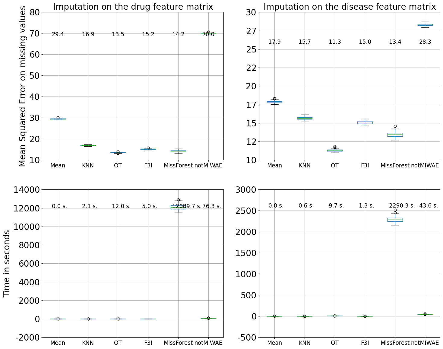
Figure 22: Imputation of missing values in the drug (left) and disease (right) feature matrices for F3I and its baselines in the Cdataset drug repurposing data set (Luo et al., 2016). The first row shows boxplots of mean-squared errors (MSE) across each algorithm’s $100$ iterations (with different random seeds). In contrast, the second row displays the runtimes (in seconds) across iterations for the imputation step. The average value of MSE and runtime is displayed above each corresponding boxplot. Abbreviations: OT: Optimal Transport-based imputer (Muzellec et al., 2020), KNN: KNN imputer with distance-associated weights (Troyanskaya et al., 2001), Mean: imputation by the feature-wise mean value.

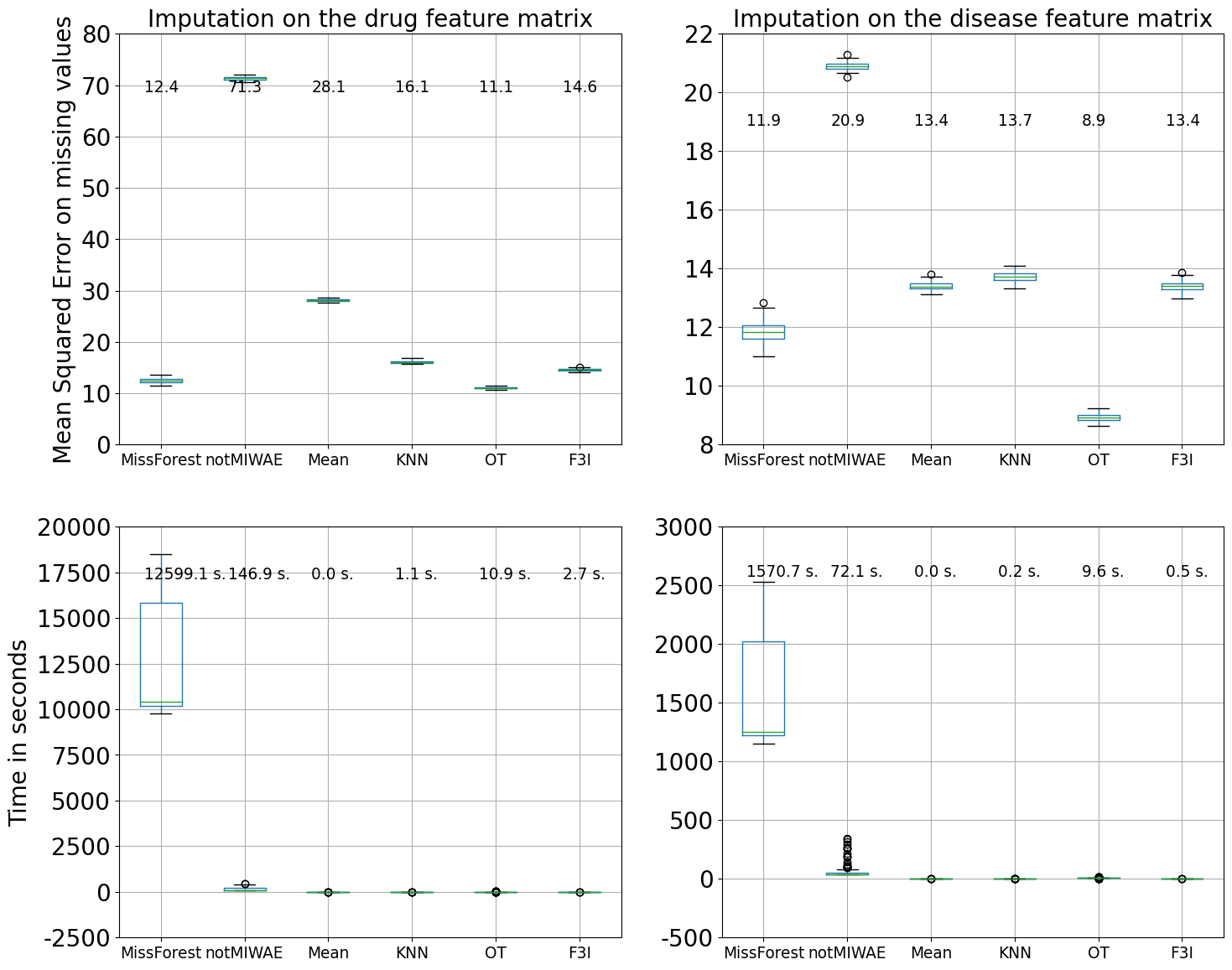
Figure 24: Imputation of missing values in the drug (left) and disease (right) feature matrices for F3I and its baselines in the Gottlieb drug repurposing data set (Luo et al., 2016). The first row shows boxplots of mean-squared errors (MSE) across each algorithm’s $100$ iterations (with different random seeds). In contrast, the second row displays the runtimes (in seconds) across iterations for the imputation step. The average value of MSE and runtime is displayed above each corresponding boxplot. Abbreviations: OT: Optimal Transport-based imputer (Muzellec et al., 2020), KNN: KNN imputer with distance-associated weights (Troyanskaya et al., 2001), Mean: imputation by the feature-wise mean value.

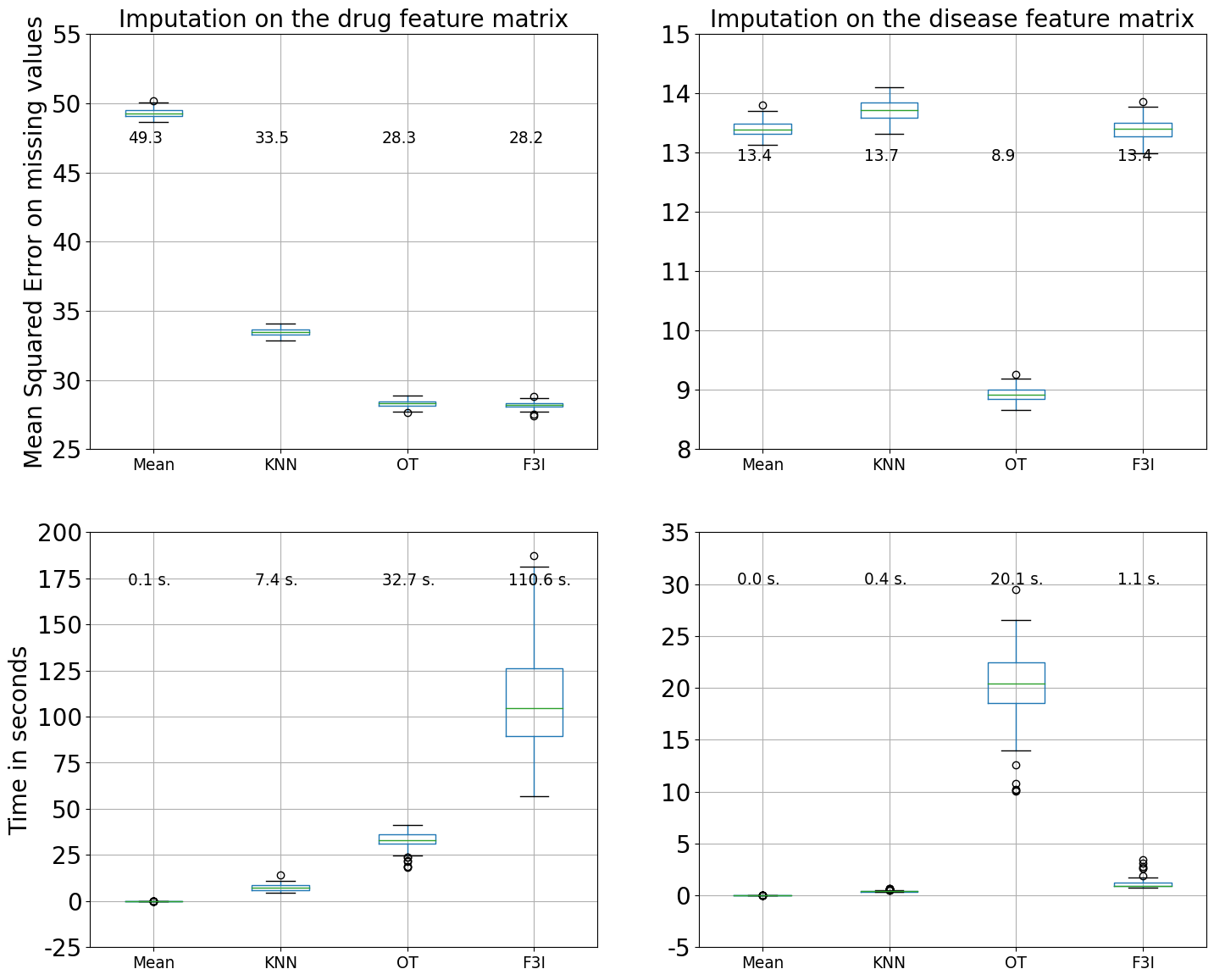
Figure 25: Imputation of missing values in the drug (left) and disease (right) feature matrices for F3I and its baselines in the PREDICT-Gottlieb drug repurposing data set (Gao et al., 2022). The first row shows boxplots of mean-squared errors (MSE) across each algorithm’s $100$ iterations (with different random seeds). In contrast, the second row displays the runtimes (in seconds) across iterations for the imputation step. The average value of MSE and runtime is displayed above each corresponding boxplot. Abbreviations: OT: Optimal Transport-based imputer (Muzellec et al., 2020), KNN: KNN imputer with distance-associated weights (Troyanskaya et al., 2001), Mean: imputation by the feature-wise mean value.

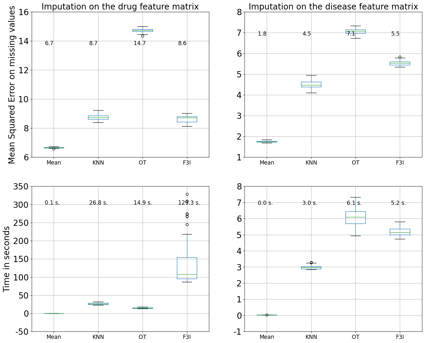
Figure 26: Imputation of missing values in the drug (left) and disease (right) feature matrices for F3I and its baselines in the TRANSCRIPT drug repurposing data set (Réda, 2023b), restricted to the $9,000$ features with highest variance across samples. The first row shows boxplots of mean-squared errors (MSE) across each algorithm’s $100$ iterations (with different random seeds). In contrast, the second row displays the runtimes (in seconds) across iterations for the imputation step. The average value of MSE and runtime is displayed above each corresponding boxplot.

We first notice that MissForest (Stekhoven & Bühlmann, 2012) and not-MIWAE (Ipsen et al., 2021) are too resource-consuming to be run on the largest data sets (see in Appendix F.2). Figure 1 reports the boxplots of mean squared errors and runtimes for drug and disease matrices in the DNdataset drug repurposing set. The full set of figures is located in Appendix F.2 (Figures 22-26).

Overall, F3I can perform on par or sometimes superior to the state-of-the-art while remaining computationally efficient, even on the largest data sets for drug repurposing. Computational efficacy is crucial for applying imputation methods to real-life data sets.

6.2 Joint imputation-classification task: MNIST data

We implement the joint imputation-classification training with the log-loss function and sigmoid classifier $\ell(\bm{x})\triangleq-y\log C_{\bm{\omega}}(\bm{x})$ mentioned in Section 5, where $y\in\{0,1\}$ is the binary class associated with sample $\bm{x}\in\mathbb{R}^{F}$. To implement PCGrad-F3I, we chain the imputation phase by F3I with an MLP classifier, which returns logits. At time $t$, the imputation part applies at a fixed set of parameters $\bm{\omega}^{t}$ with the learner losses defined in Equation (2).

We compare the performance of PCGrad-F3I with adding a NeuMiss block (Le Morvan et al., 2020) or performing an imputation by the mean (“Mean”) before the classifier. The NeuMiss block features linear layers alternating with multiplications by the missingness pattern. Similarly to PCGrad-F3I, we chain those blocks (a shared-weights NeuMiss block (Le Morvan et al., 2021) or imputation by the mean) with an MLP, which returns logits.

The criterion for training the models is the log loss, and we split the samples into training ($70\%$), validation ($20\%$), and testing ($10\%$) sets, where the former two sets are used for training the MLP, and the performance metrics are computed on the latter set. We consider the classical Area Under the Curve (AUC) on the test set (hidden during training) as the performance metric for the binary classification task. Further experimental details can be found in Appendix F.

We consider the MNIST dataset (LeCun et al., 1998), which comprises grayscale images of $25\times 25$ pixels of handwritten digits. We restrict our study to images annotated with class 0 or 1 to get a binary classification problem. We remove pixels at random with probability $50\%$ using a MCAR mechanism, and we run the MLP with the following hyperparameters: MLP depth: 5 layers, number of epochs: 10. We run PCGradF3I with $\beta=0.142$, $T=30$, $K=19$ and $\eta=0.023$. Those hyperparameters were fine-tuned by the approach described in Appendix F.2.

Table 1 displays the numerical results across $100$ iterations (different random seeds). The empirical performance of PCGrad-F3I on classification tasks is superior to NeuMiss (Le Morvan et al., 2020) or applying a mean imputation before the prediction. This might be explained by the fact that, for this classification of images, a good imputation quality is crucial and is the most informative of the ground truth class. See Figure 2 for comparing the imputation performed by Mean and PCGradF3I. As more and more pixels are missing, the mean imputation struggles to preserve the correct shapes, whereas PCGradF3I retrieves them successfully.

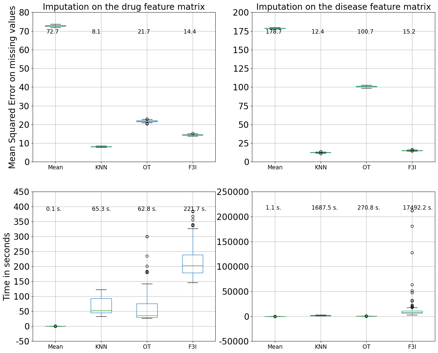
Figure 1: Imputation of missing values in the drug (left) and disease (right) feature matrices for F3I and its baselines in the DNdataset drug repurposing data set (Gao et al., 2022). Average values are reported at the top of each corresponding boxplot. Abbreviations: OT: Optimal Transport-based imputer (Muzellec et al., 2020), KNN: KNN imputer with distance-associated weights (Troyanskaya et al., 2001), Mean: imputation by the feature-wise average.

Table 1: Area Under the Curve (AUC) values (average $\pm$ standard deviation) in the testing subset in MNIST, which is hidden during the training phase, for $100$ iterations.

Algorithm	AUC on held-out set
Mean	0.640 $\pm$0.180
NeuMiss	0.989 $\pm$0.069
PCGradF3I (ours)	0.990 $\pm$0.094

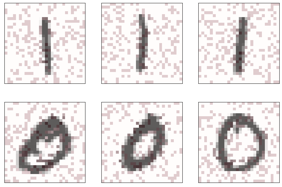
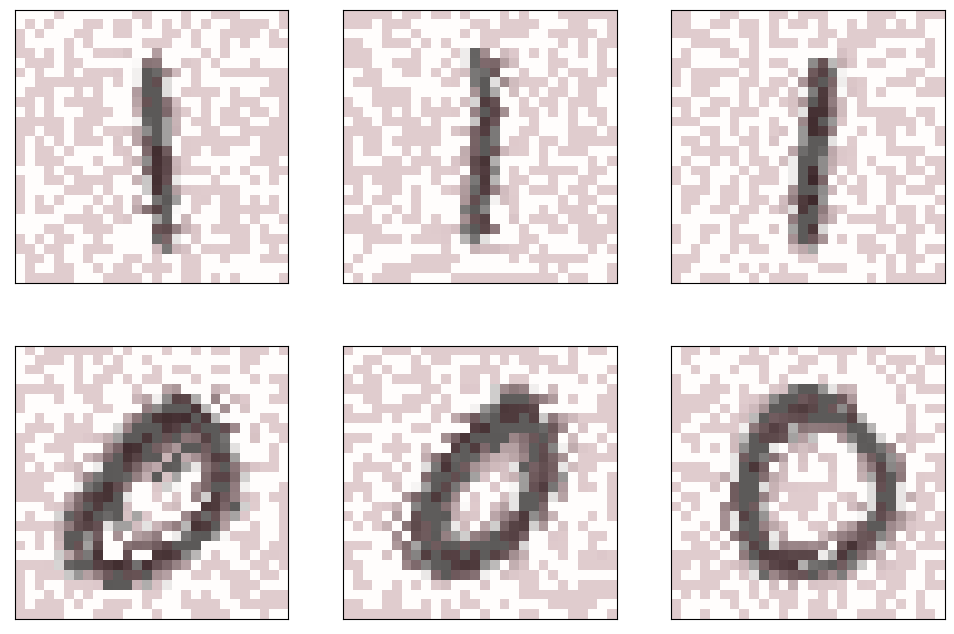
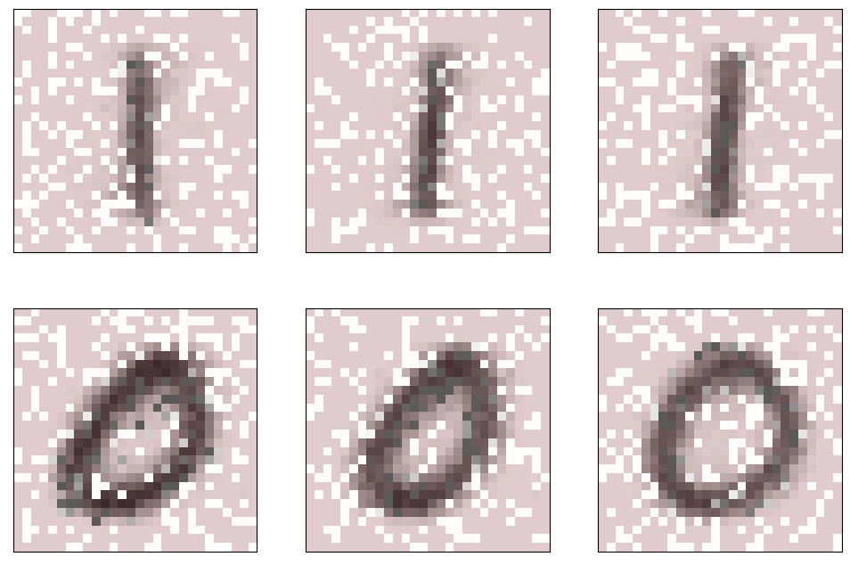
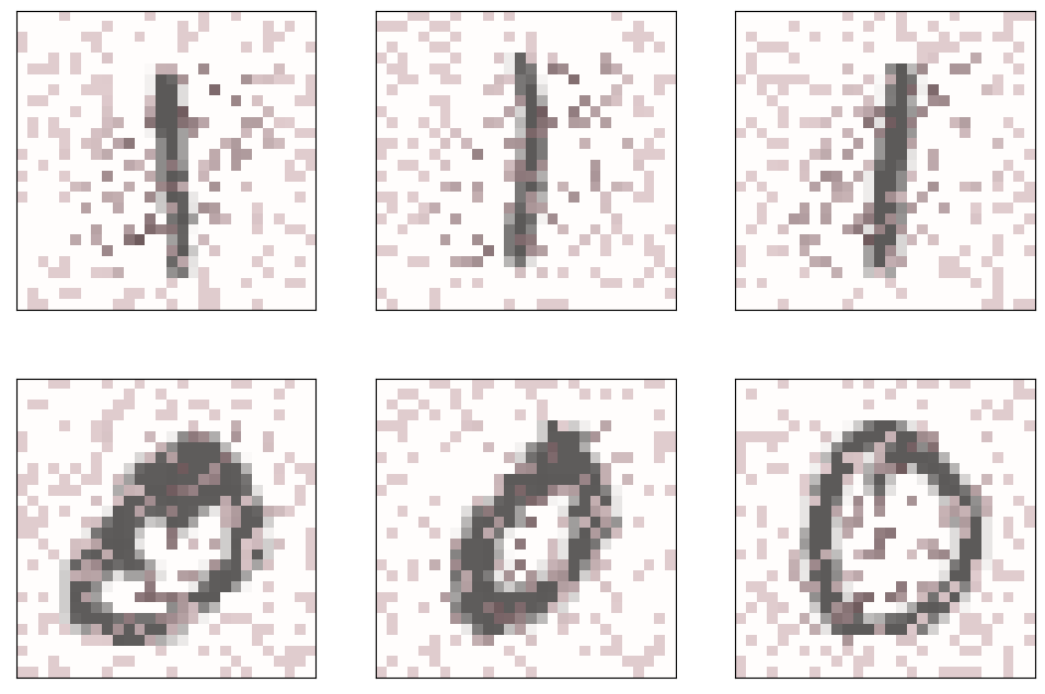
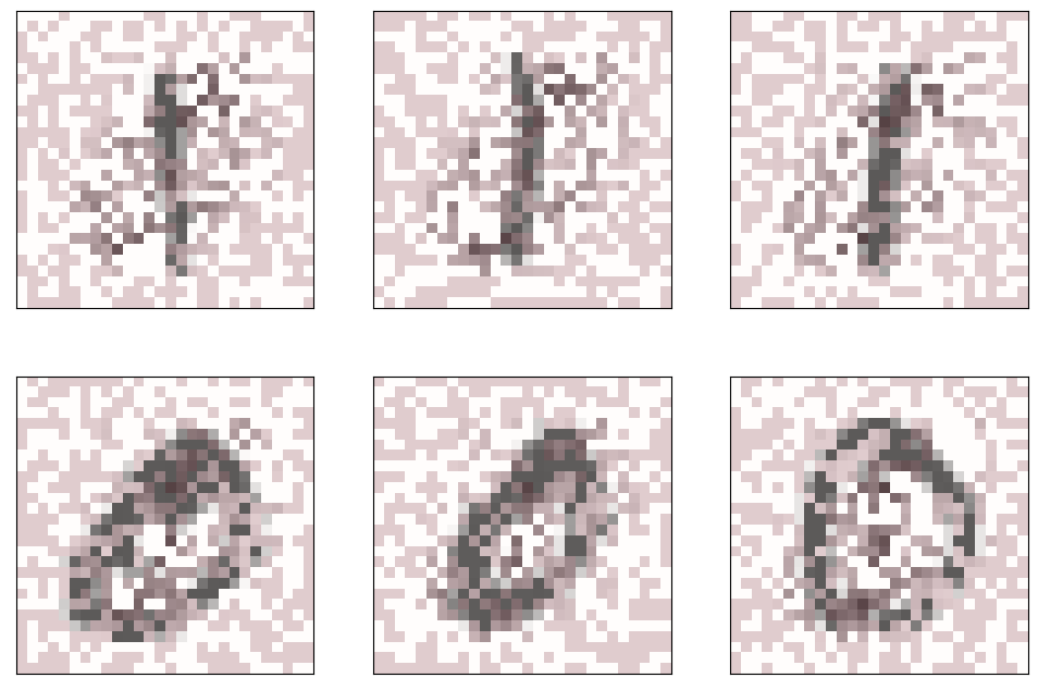
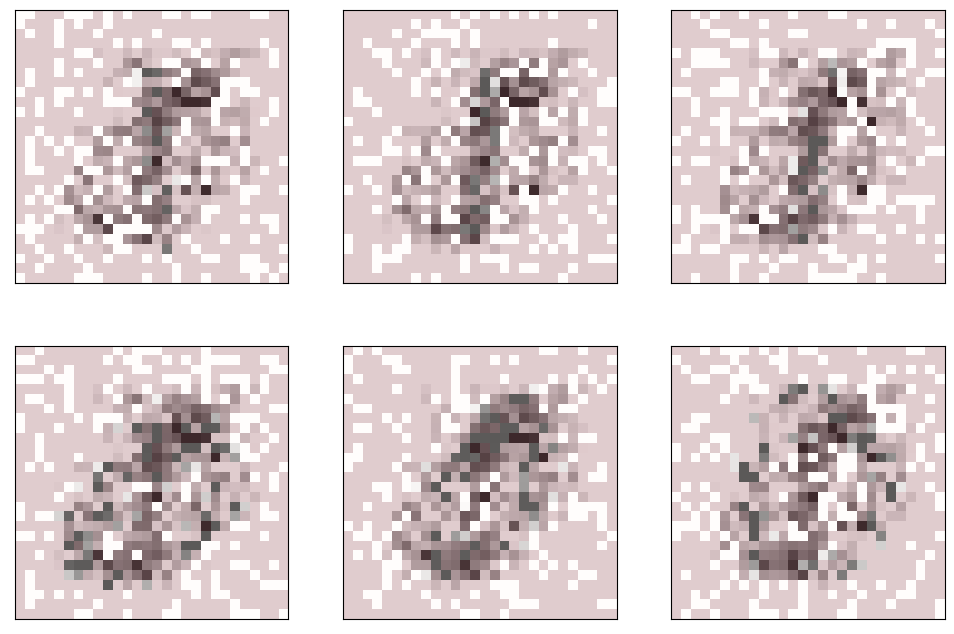
Figure 2: Imputed grayscale images by F3I (first two rows) or mean imputation (last two rows) for the first $6$ samples (trained on the first 600 samples of MNIST with the selected hyperparameters) with MCAR-missing pixels, with missingness frequencies in $\{25\%,50\%,75\%\}$. Columns 1 to 3 correspond to $p^{\text{miss}}=25\%$, columns 4 to 6 to $p^{\text{miss}}=50\%$, and columns 7 to 9 to $p^{\text{miss}}=75\%$. Positions of red pixels represent missing pixels during the training phase which are imputed by either F3I or mean imputation.

7 Discussion

This paper introduces an online algorithm named F3I which iteratively improves a K-nearest neighbor imputation by fine-tuning the weights corresponding to each of the $K$ closest neighbors. Interestingly, this algorithm does not need to train by hiding some of the available values, and can be jointly trained with a downstream task depending on whether the end goal is a good imputation quality or a good downstream performance. Empirically, this algorithm remains computationally tractable even under a large number of features. The experimental code and the implementation of F3I (and PCGrad-F3I) are provided as supplementary material. However, there are a few limitations for F3I. First, the K-nearest neighbor imputation is costly when the number of samples is very large. Second, F3I can only be used on continuous variables, and, finally, the theoretical guarantees derived in Theorems 4.2-4.5 only hold for one-dimensional Gaussian data.

The approach combining online learning and density ratio estimation is a simple idea that could be improved further, notably to perhaps remove the linear term in the number of iterations in Theorem 4.5. In particular, the density ratio estimation step might benefit from the classifier-based approach developed in BORE (Tiao et al., 2021), in particular in the version of F3I where a k-d tree would be rebuilt at every iteration to consider density $D_{t}$ on points $\{(\bm{x}^{t})_{1},\dots,(\bm{x}^{t})_{N}\}$ instead of the density estimated on naively imputed points.

Impact Statement

This paper presents work whose goal is to advance the field of Machine Learning. There are many potential societal consequences of our work, none which we feel must be specifically highlighted here.

Appendix A Properties of the objective function G

Proposition A.1.

Continuity and derivability of $G$ (Proposition 3.8). $G$ is continuous and infinitely derivable with respect to $\bm{\alpha}\in\triangle_{K}$.

Proof.

$G$ is a composition and sum of indefinitely derivable functions on their respective domains, which are compatible: $\log$ on $\mathbb{R}^{+*}$, $\exp$ on $\mathbb{R}$ of image domain $\mathbb{R}^{+*}$, $\|\cdot\|_{2}$ and the linear imputation model (Algorithm 1) on $\mathbb{R}$ with image domain $\mathbb{R}$. ∎

Proposition A.2.

Strict concavity of $G$ in $\bm{\alpha}$ (Proposition 3.9). Assume that $\eta<4KN$. Then there exists $h_{0}>0$ such that for all $h\geq h_{0}$, $G$ is strictly concave in $\bm{\alpha}$.

We aim to show that a value of $h_{0}$ always exists such that, for $h\geq 0$, the Hessian matrix of $G$ with respect to $\bm{\alpha}$ is negative (semi-)definite. First, we compute the Hessian matrix of $G$.

Lemma A.3.

Gradient of $G$ with respect to $\bm{\alpha}$. The gradient $\nabla_{\bm{\alpha}}G(\bm{\alpha},X)\in\mathbb{R}^{K}$ at $\bm{\alpha}\in\mathbb{R}^{K}$ and fixed $X\in\mathbb{R}^{N\times F}$ is

$$\nabla_{\bm{\alpha}}G(\bm{\alpha},X)=-\sum_{i\leq N}\frac{D_{0}(\bm{x}_{i}(\bm{\alpha}))^{-1}}{2hN^{2}(\sqrt{2\pi}h)^{F}}\left(\sum_{j\leq N}e^{-\frac{1}{4h}\|\bm{x}_{i}(\bm{\alpha})-(\bm{x}^{0})_{j}\|^{2}_{2}}\left(\bm{x}_{i}(\bm{\alpha})-(\bm{x}^{0})_{j}\right)\right)^{\intercal}\widetilde{Z}^{n_{i}}-2\eta\bm{\alpha}\;,$$

where $n^{i}\triangleq(n^{i}_{1},n^{i}_{2},\dots,n^{i}_{K})$ is the set of indices of the K-nearest neighbors of $\bm{x}_{i}$ among the reference set $Z=\{(\bm{x}^{0})_{1},(\bm{x}^{0})_{2},\dots,(\bm{x}^{0})_{N}\}$, $\widetilde{Z}^{n_{i}}\in\mathbb{R}^{F\times K}$ where the $k^{\text{th}}$ column of $\widetilde{Z}^{n_{i}}$ is defined as $(\widetilde{\bm{z}}^{n_{i}})^{f}_{k}=0$ if $m^{f}_{i}=0$, $(\widetilde{z}^{n_{i}})^{f}_{k}=(x^{0})^{f}_{n^{i}_{k}}$ otherwise. That is, $(\widetilde{\bm{z}}^{n_{i}})_{k}$ is equal to the $k^{\text{th}}$ closest neighbor of $\bm{x}_{i}$ (by increasing order of distance) on missing coordinates of $\bm{x}_{i}$, and equal to zero otherwise.

Proof.

The gradient of $G$ at $\bm{\alpha}\in\triangle_{K}$ for a fixed $X\in\mathbb{R}^{N\times F}$ is

$$\nabla_{\bm{\alpha}}G(\bm{\alpha},X) = \sum_{i\leq N}\frac{D_{0}(\bm{x}_{i}(\bm{\alpha}))^{-1}}{N}\nabla_{\bm{\alpha}}D_{0}(\bm{x}_{i}(\bm{\alpha}))-0-2\eta\bm{\alpha}$$

$$\nabla_{\bm{\alpha}}D_{0}(\bm{x}_{i}(\bm{\alpha})) = -\frac{1}{4hN(\sqrt{2\pi}h)^{F}}\sum_{j\leq N}e^{-\frac{1}{4h}\|\bm{x}_{i}(\bm{\alpha})-(\bm{x}^{0})_{j}\|^{2}_{2}}\nabla_{\bm{\alpha}}\|\bm{x}_{i}(\bm{\alpha})-(\bm{x}^{0})_{j}\|^{2}_{2}$$

$$\nabla_{\bm{\alpha}}\|\bm{x}_{i}(\bm{\alpha})-(\bm{x}^{0})_{j}\|^{2}_{2} = 2\left(\bm{x}_{i}(\bm{\alpha})-(\bm{x}^{0})_{j}\right)\nabla_{\bm{\alpha}}\bm{x}_{i}(\bm{\alpha})\text{ and }\nabla_{\bm{\alpha}}\bm{x}_{i}(\bm{\alpha})=\widetilde{Z}^{n_{i}}\;.$$

∎

Lemma A.4.

Hessian matrix of $G$ with respect to $\bm{\alpha}$. Let us denote for any $i,j\leq N$ and $\bm{\alpha}\in\triangle_{K}$

• $u^{ij}_{\bm{\alpha}}\triangleq e^{-\frac{1}{4h}\|\bm{x}_{i}(\bm{\alpha})-(\bm{x}^{0})_{j}\|^{2}_{2}}$ and $U^{i}_{\bm{\alpha}}\triangleq\sum_{j\leq N}u^{ij}_{\bm{\alpha}}=N(\sqrt{2\pi}h)^{F}D_{0}(\bm{x}_{i}(\bm{\alpha}))$,

• $S^{i}_{\bm{\alpha}}\triangleq\sum_{j\leq N}u^{ij}_{\bm{\alpha}}(\bm{x}_{i}(\bm{\alpha})-(\bm{x}^{0})_{j})$ and $T^{i}_{\bm{\alpha}}\triangleq\sum_{j\leq N}u^{ij}_{\bm{\alpha}}(\|\bm{x}_{i}(\bm{\alpha})-(\bm{x}^{0})_{j}\|^{2}_{2}-2h)$.

Then the coefficient at position $(k,q)$ of Hessian matrix $\nabla^{2}_{\bm{\alpha}}G(\bm{\alpha},X)\in\mathbb{R}^{K\times K}$ at $\bm{\alpha}$ and fixed X is

$$\frac{\partial^{2}G(\bm{\alpha},X)}{\partial\alpha_{k}\partial\alpha_{q}} = \sum_{i\leq N}\left(\frac{T^{i}_{\bm{\alpha}}}{NU^{i}_{\bm{\alpha}}}-\frac{(S^{i}_{\bm{\alpha}})^{\intercal}S^{i}_{\bm{\alpha}}}{4h^{2}(U^{i}_{\bm{\alpha}})^{2}}\right)(\widetilde{\bm{z}}^{n_{i}})_{q}^{\intercal}(\widetilde{\bm{z}}^{n_{i}})_{k}-\eta\delta(q=k)\;.$$

Proof.

According to Lemma A.3, for any $k\leq K$

$$\frac{\partial G(\bm{\alpha},X)}{\partial\alpha_{k}}=-\sum_{i\leq N}\frac{D_{0}(\bm{x}_{i}(\bm{\alpha}))^{-1}}{2hN^{2}(\sqrt{2\pi}h)^{F}}(S^{i}_{\bm{\alpha}})^{\intercal}(\widetilde{\bm{z}}^{n_{i}})_{k}-2\eta\alpha_{k}\;.$$

This implies that

$$\frac{\partial^{2}G(\bm{\alpha},X)}{\partial\alpha_{k}\partial\alpha_{q}}+2\eta\delta(q=k) = \sum_{i\leq N}\frac{-D_{0}(\bm{x}_{i}(\bm{\alpha}))^{-1}}{2hN^{2}(\sqrt{2\pi}h)^{F}}\Big{(}\left(\frac{\partial S^{i}_{\bm{\alpha}}}{\partial\alpha_{q}}\right)^{\intercal}(\widetilde{\bm{z}}^{n_{i}})_{k}$$

$$-\frac{(S^{i}_{\bm{\alpha}})^{\intercal}(\widetilde{\bm{z}}^{n_{i}})_{k}}{D_{0}(\bm{x}_{i}(\bm{\alpha}))}\frac{\partial D_{0}(\bm{x}_{i}(\bm{\alpha}))}{\partial\alpha_{q}}\Big{)}$$

And then

$$\frac{\partial S^{i}_{\bm{\alpha}}}{\partial\alpha_{q}} = \frac{-1}{4h}\sum_{j\leq N}e^{-\frac{1}{4h}\|\bm{x}_{i}(\bm{\alpha})-(\bm{x}^{0})_{j}\|^{2}_{2}}\Big{(}\frac{\partial\|\bm{x}_{i}(\bm{\alpha})-(\bm{x}^{0})_{j}\|^{2}_{2}}{\partial\alpha_{q}}\Big{)}^{\intercal}(\bm{x}_{i}(\bm{\alpha})-(\bm{x}^{0})_{j})$$

$$+ \sum_{j\leq N}e^{-\frac{1}{4h}\|\bm{x}_{i}(\bm{\alpha})-(\bm{x}^{0})_{j}\|^{2}_{2}}\frac{\partial\bm{x}_{i}(\bm{\alpha})}{\partial\alpha_{q}}$$

$$= \frac{-1}{2h}\sum_{j\leq N}e^{-\frac{1}{4h}\|\bm{x}_{i}(\bm{\alpha})-(\bm{x}^{0})_{j}\|^{2}_{2}}(\widetilde{\bm{z}}^{n_{i}})^{\intercal}_{q}(\bm{x}_{i}(\bm{\alpha})-(\bm{x}^{0})_{j})^{\intercal}\left(\bm{x}_{i}(\bm{\alpha})-(\bm{x}^{0})_{j}\right)$$

$$+ \sum_{j\leq N}e^{-\frac{1}{4h}\|\bm{x}_{i}(\bm{\alpha})-(\bm{x}^{0})_{j}\|^{2}_{2}}(\widetilde{\bm{z}}^{n_{i}})^{\intercal}_{q}$$

That is,

$$\frac{\partial S^{i}_{\bm{\alpha}}}{\partial\alpha_{q}} = (\widetilde{\bm{z}}^{n_{i}})^{\intercal}_{q}\underbrace{\left(\sum_{j\leq N}e^{-\frac{1}{4h}\|\bm{x}_{i}(\bm{\alpha})-(\bm{x}^{0})_{j}\|^{2}_{2}}\Big{(}1-(2h)^{-1}\|\bm{x}_{i}(\bm{\alpha})-(\bm{x}^{0})_{j}\|^{2}_{2}\Big{)}\right)}_{=-2hT^{i}_{\bm{\alpha}}}$$

$$\frac{\partial D_{0}(\bm{x}_{i}(\bm{\alpha}))}{\partial\alpha_{q}} = -\frac{(S^{i}_{\bm{\alpha}})^{\intercal}(\widetilde{\bm{z}}^{n_{i}})_{q}}{2hN(\sqrt{2\pi}h)^{F}}\text{ according to Lemma~\ref{lem:gradient_G}}\;.$$

Moreover, since $S^{i}_{\bm{\alpha}},(\widetilde{\bm{z}}^{n_{i}})_{k}\in\mathbb{R}^{F}$ for any $k\leq K$

$$(S^{i}_{\bm{\alpha}})^{\intercal}(\widetilde{\bm{z}}^{n_{i}})_{k}(S^{i}_{\bm{\alpha}})^{\intercal}(\widetilde{\bm{z}}^{n_{i}})_{q}=\underbrace{(S^{i}_{\bm{\alpha}})^{\intercal}(\widetilde{\bm{z}}^{n_{i}})_{q}}_{=(\widetilde{\bm{z}}^{n_{i}})_{q}^{\intercal}S^{i}_{\bm{\alpha}}}(S^{i}_{\bm{\alpha}})^{\intercal}(\widetilde{z}^{n^{i}})_{k}=(\widetilde{\bm{z}}^{n_{i}})_{q}^{\intercal}(S^{i}_{\bm{\alpha}})^{\intercal}S^{i}_{\bm{\alpha}}(\widetilde{\bm{z}}^{n_{i}})_{k}\;.$$

∎

Then, to show that $G$ is (strictly) concave, it is enough to show that the Hessian matrix $\nabla^{2}_{\bm{\alpha}}G(\bm{\alpha},X)$ is negative semi-definite (or definite). We assume that $\eta<4S^{2}K=4K$ (using Assumption 3.6), which is the case for most realistic settings.

Proof.

Let us denote $\bm{x}^{ij}_{\bm{\alpha}}\triangleq x^{i}_{\bm{\alpha}}-(\bm{x}^{0})_{j}$ for any $i,j\leq N$. Then

$$\frac{T^{i}_{\bm{\alpha}}}{NU^{i}_{\bm{\alpha}}}-\frac{(S^{i}_{\bm{\alpha}})^{\intercal}S^{i}_{\bm{\alpha}}}{4h^{2}(U^{i}_{\bm{\alpha}})^{2}} = \frac{T^{i}_{\bm{\alpha}}}{NU^{i}_{\bm{\alpha}}}-\frac{1}{4h^{2}}\left(\sum_{j,j^{\prime}\leq N}\frac{u^{ij}_{\bm{\alpha}}}{U^{i}_{\bm{\alpha}}}\frac{u^{ij^{\prime}}_{\bm{\alpha}}}{U^{i}_{\bm{\alpha}}}(\bm{x}^{ij}_{\bm{\alpha}})^{\intercal}\bm{x}^{ij^{\prime}}_{\bm{\alpha}}\right)\;.$$ (3)

Now consider $(\bm{x}^{ij}_{\bm{\alpha}})^{\intercal}\bm{x}^{ij^{\prime}}_{\bm{\alpha}}=\langle\bm{x}_{i}(\bm{\alpha})-(\bm{x}^{0})_{j},\ \bm{x}_{i}(\bm{\alpha})-(\bm{x}^{0})_{j^{\prime}}\rangle$. From the triangle equality, we have, for all $j,j^{\prime}\leq N$

$$\langle\bm{x}_{i}(\bm{\alpha})-(\bm{x}^{0})_{j},\ \bm{x}_{i}(\bm{\alpha})-(\bm{x}^{0})_{j^{\prime}}\rangle=\frac{1}{2}(\|\bm{x}_{i}(\bm{\alpha})-(\bm{x}^{0})_{j}\|^{2}_{2}+\|\bm{x}_{i}(\bm{\alpha})-(\bm{x}^{0})_{j^{\prime}}\|^{2}_{2}-\|(\bm{x}^{0})_{j}-(\bm{x}^{0})_{j^{\prime}}\|^{2}_{2})\;.$$

We plug this inequality into Equation (3)

$$\frac{T^{i}_{\bm{\alpha}}}{NU^{i}_{\bm{\alpha}}}-\frac{(S^{i}_{\bm{\alpha}})^{\intercal}S^{i}_{\bm{\alpha}}}{4h^{2}(U^{i}_{\bm{\alpha}})^{2}} =\frac{T^{i}_{\bm{\alpha}}}{NU^{i}_{\bm{\alpha}}}+\frac{1}{8h^{2}}\sum_{j,j^{\prime}\leq N}\frac{u^{ij}_{\bm{\alpha}}}{U^{i}_{\bm{\alpha}}}\frac{u^{ij^{\prime}}_{\bm{\alpha}}}{U^{i}_{\bm{\alpha}}}\|(\bm{x}^{0})_{j}-(\bm{x}^{0})_{j^{\prime}}\|^{2}_{2}$$

$$-\underbrace{\frac{1}{8h^{2}}\sum_{j,j^{\prime}\leq N}\frac{u^{ij}_{\alpha}}{U^{i}_{\alpha}}\frac{u^{ij^{\prime}}_{\alpha}}{U^{i}_{\alpha}}(\|\bm{x}_{i}(\bm{\alpha})-(\bm{x}^{0})_{j}\|^{2}_{2}+\|\bm{x}_{i}(\bm{\alpha})-(\bm{x}^{0})_{j^{\prime}}\|^{2}_{2})}_{\geq 0}$$

$$\leq\frac{T^{i}_{\bm{\alpha}}}{NU^{i}_{\bm{\alpha}}}+\frac{1}{8h^{2}}\sum_{j,j^{\prime}\leq N}\frac{u^{ij}_{\bm{\alpha}}}{U^{i}_{\bm{\alpha}}}\frac{u^{ij^{\prime}}_{\bm{\alpha}}}{U^{i}_{\bm{\alpha}}}\|(\bm{x}^{0})_{j}-(\bm{x}^{0})_{j^{\prime}}\|^{2}_{2}\;.$$

Obviously $\frac{u^{ij}_{\bm{\alpha}}}{U^{i}_{\bm{\alpha}}}\leq 1$. Moreover, since Assumption 3.6 gives $\|(\bm{x}^{0})_{j}\|^{2}_{2}\leq S$ and $\|\bm{x}_{j}(\bm{\alpha})\|^{2}_{2}\leq S$ (using Jensen’s inequality) for any $j\leq N$,

$$\frac{T^{i}_{\bm{\alpha}}}{NU^{i}_{\bm{\alpha}}}-\frac{(S^{i}_{\bm{\alpha}})^{\intercal}S^{i}_{\bm{\alpha}}}{4h^{2}(U^{i}_{\bm{\alpha}})^{2}} \leq\frac{T^{i}_{\bm{\alpha}}}{NU^{i}_{\bm{\alpha}}}+\frac{2N^{2}S}{8h^{2}}=\frac{T^{i}_{\bm{\alpha}}}{NU^{i}_{\bm{\alpha}}}+\frac{N^{2}S}{4h^{2}}$$

$$=\sum_{j\leq N}\frac{u^{ij}_{\bm{\alpha}}}{NU^{i}_{\bm{\alpha}}}(\|\bm{x}^{i}(\bm{\alpha})-(\bm{x}^{0})_{j}\|^{2}_{2}-2h)+\frac{NS}{4h^{2}}$$

$$\leq\frac{1}{N}\sum_{j\leq N}\|\bm{x}^{i}(\bm{\alpha})-(\bm{x}^{0})_{j}\|^{2}_{2}-2h+\frac{N^{2}S}{4h^{2}}$$

$$\leq\frac{1}{N}\sum_{j\leq N}(\|\bm{x}^{i}(\bm{\alpha})||^{2}_{2}+\|(\bm{x}^{0})_{j}\|^{2}_{2})-2h+\frac{N^{2}S}{4h^{2}}$$

$$\leq 2S-2h+N^{2}S(4h^{2})^{-1}\;.$$

We set $C(h)\triangleq h^{-2}(-2h^{3}+2Sh^{2}+N^{2}S/4)$, and fix $\bm{v}\in\mathbb{R}^{K}$. Then

$$\bm{v}^{\intercal}\nabla^{2}_{\bm{\alpha}}G(\bm{\alpha},X)\bm{v} =-\eta\|\bm{v}\|^{2}_{2}+\sum_{i\leq N}\left(\frac{T^{i}_{\bm{\alpha}}}{NU^{i}_{\bm{\alpha}}}-\frac{(S^{i}_{\bm{\alpha}})^{\intercal}S^{i}_{\bm{\alpha}}}{4h^{2}(U^{i}_{\bm{\alpha}})^{2}}\right)(\bm{v}^{\intercal}(\widetilde{Z}^{n_{i}})^{\intercal}\widetilde{Z}^{n_{i}}\bm{v})$$

$$\leq-\eta\|\bm{v}\|^{2}_{2}+C(h)\sum_{i\leq N}\|\widetilde{Z}^{n_{i}}\bm{v}\|^{2}_{2}$$

so, using Technical lemma 1 (proven below),

$$\bm{v}^{\intercal}\nabla^{2}_{\bm{\alpha}}G(\bm{\alpha},X)\bm{v}\leq\|\bm{v}\|^{2}_{2}(2KSC(h)-\eta)=\|\bm{v}\|^{2}_{2}\times h^{-2}\left(-4KSh^{3}+(4S^{2}K-\eta)h^{2}+\frac{KN^{2}S^{2}}{2}\right)\;.$$

Then we choose $h>0$ such that $\bm{v}^{\intercal}\nabla^{2}_{\bm{\alpha}}G(\bm{\alpha},X)\bm{v}<0$. That is

$$-4KSh^{3}+(4S^{2}K-\eta)h^{2}+\frac{KN^{2}S^{2}}{2}<0\Leftrightarrow-2h^{3}+\frac{4S^{2}K-\eta}{2KS}h^{2}+\frac{N^{2}S}{4}<0\;.$$ (4)

Under the assumption of $\eta<4S^{2}K$, this is equivalent to analyzing the following cubic equation

$$-2h^{3}+bh^{2}+c=0\text{ where }b,c>0\;.$$

The cubic equation above admits three roots and at least one real root. We show that at least one real root is positive (thus, corresponds to a valid bandwidth). To show that there exists $h>0$ such that $-2h^{3}+bh^{2}+c<0$, it is enough to show that there exists $h^{\prime}\in\mathbb{R}$ such that on $[h^{\prime},+\inf)$, continuous and infinitely derivable function $x\mapsto-2x^{3}+bx^{2}+c$ is strictly decreasing. We have $\frac{\text{d}}{\text{d}h}(-2h^{3}+bh^{2}+c)=-6h^{2}+2bh$ with roots $0$ and $b/3$, and $\frac{\text{d}^{2}}{\text{d}^{2}h}(-2h^{3}+bh^{2}+c)=-12h+2b$, and then $-12\times 0+2b=2b>0$ and $-12\times\frac{b}{3}+2b=-2b<0$. The analysis of the behavior of $x\mapsto-2x^{3}+bx^{2}+c$ then shows that the condition is fulfilled for $h^{\prime}=b/3>0$.

Finally, the value of $h$ can be found through the known closed-form expressions of roots of the rightmost cubic polynomial in $h$ in Equation (4). ∎

Proposition A.5.

The gradient of $G(\cdot,X)$ for any $X\in\mathbb{R}^{N\times F}$ is Lipschitz-continuous (Proposition 3.10). There exists a positive constant $H$ such that

$$\|\nabla_{\bm{\alpha}}G(\bm{\alpha},X)-\nabla_{\bm{\alpha}}G(\bm{\alpha}^{\prime},X)\|_{2}\leq H\|\bm{\alpha}-\bm{\alpha}^{\prime}\|_{2}\;.$$

Proof.

According to Lemma A.3, and using notation from Lemma A.4, for any $X\in\mathbb{R}^{N\times F}$ and $\bm{\alpha}\in\triangle_{K}$

$$\nabla_{\bm{\alpha}}G(\bm{\alpha},X)=-\frac{1}{2hN}\sum_{i,j\leq N}\frac{u^{ij}_{\bm{\alpha}}}{U^{i}_{\bm{\alpha}}}\left(\bm{x}_{i}(\bm{\alpha})-(\bm{x}^{0})_{j}\right)^{\intercal}\widetilde{Z}^{n_{i}}-2\eta\bm{\alpha}\;.$$

Then for any $\bm{\alpha},\bm{\alpha}^{\prime}\in\triangle_{K}$

$$\|\nabla_{\bm{\alpha}}G(\bm{\alpha},X)-\nabla_{\bm{\alpha}}G(\bm{\alpha}^{\prime},X)\|_{2}$$

$$=\|-\frac{1}{2hN}\sum_{i,j\leq N}\Big{(}\frac{u^{ij}_{\bm{\alpha}}}{U^{i}_{\bm{\alpha}}}\left(\bm{x}_{i}(\bm{\alpha})-(\bm{x}^{0})_{j}\right)-\frac{u^{ij}_{\bm{\alpha}^{\prime}}}{U^{i}_{\bm{\alpha}^{\prime}}}\left(\bm{x}_{i}(\bm{\alpha}^{\prime})-(\bm{x}^{0})_{j}\right)\Big{)}^{\intercal}\widetilde{Z}^{n_{i}}-2\eta(\bm{\alpha}-\bm{\alpha}^{\prime})\|_{2}$$

$$\leq\frac{1}{2hN}\sum_{i\leq N}\|\sum_{j\leq N}\Big{(}\frac{u^{ij}_{\bm{\alpha}}}{U^{i}_{\bm{\alpha}}}\left(\bm{x}_{i}(\bm{\alpha})-(\bm{x}^{0})_{j}\right)-\frac{u^{ij}_{\bm{\alpha}^{\prime}}}{U^{i}_{\bm{\alpha}^{\prime}}}\left(\bm{x}_{i}(\bm{\alpha}^{\prime})-(\bm{x}^{0})_{j}\right)\Big{)}^{\intercal}\widetilde{Z}^{n_{i}}\|_{2}+2\eta\|\bm{\alpha}-\bm{\alpha}^{\prime}\|_{2}$$

$$\leq\frac{1}{2hN}\sum_{i\leq N}\|\sum_{j\leq N}\frac{u^{ij}_{\bm{\alpha}}}{U^{i}_{\bm{\alpha}}}\left(\bm{x}_{i}(\bm{\alpha})-(\bm{x}^{0})_{j}\right)-\frac{u^{ij}_{\bm{\alpha}^{\prime}}}{U^{i}_{\bm{\alpha}^{\prime}}}\left(\bm{x}_{i}(\bm{\alpha}^{\prime})-(\bm{x}^{0})_{j}\right)\|_{2}\sqrt{2KS}+2\eta\|\bm{\alpha}-\bm{\alpha}^{\prime}\|_{2}$$

(using the Cauchy-Schwartz inequality and Technical lemma 1)

$$=\frac{\sqrt{KS}}{\sqrt{2}hN}\sum_{i\leq N}\|\sum_{j\leq N}\frac{u^{ij}_{\bm{\alpha}}}{U^{i}_{\bm{\alpha}}}\bm{x}_{i}(\bm{\alpha})-\frac{u^{ij}_{\bm{\alpha}^{\prime}}}{U^{i}_{\bm{\alpha}^{\prime}}}\bm{x}_{i}(\bm{\alpha}^{\prime})+\Big{(}\frac{u^{ij}_{\bm{\alpha}^{\prime}}}{U^{i}_{\bm{\alpha}^{\prime}}}-\frac{u^{ij}_{\bm{\alpha}}}{U^{i}_{\bm{\alpha}}}\Big{)}(\bm{x}^{0})_{j}\|_{2}+2\eta\|\bm{\alpha}-\bm{\alpha}^{\prime}\|_{2}$$

$$=_{U^{i}_{\bm{\alpha}}=\sum_{j}u^{ij}_{\bm{\alpha}}}\frac{\sqrt{KS}}{\sqrt{2}hN}\sum_{i\leq N}\|\bm{x}_{i}(\bm{\alpha})-\bm{x}_{i}(\bm{\alpha}^{\prime})+\sum_{j\leq N}\Big{(}\frac{u^{ij}_{\bm{\alpha}^{\prime}}}{U^{i}_{\bm{\alpha}^{\prime}}}-\frac{u^{ij}_{\bm{\alpha}}}{U^{i}_{\bm{\alpha}}}\Big{)}(\bm{x}^{0})_{j}\|_{2}+2\eta\|\bm{\alpha}-\bm{\alpha}^{\prime}\|_{2}$$

$$\leq\frac{\sqrt{KS}}{\sqrt{2}hN}\sum_{i\leq N}\big{(}\sqrt{S}\|\bm{\alpha}-\bm{\alpha}^{\prime}\|_{2}+\|\sum_{j\leq N}\Big{(}\frac{u^{ij}_{\bm{\alpha}^{\prime}}}{U^{i}_{\bm{\alpha}^{\prime}}}-\frac{u^{ij}_{\bm{\alpha}}}{U^{i}_{\bm{\alpha}}}\Big{)}(\bm{x}^{0})_{j}\|_{2}\big{)}+2\eta\|\bm{\alpha}-\bm{\alpha}^{\prime}\|_{2}$$

$$\leq\frac{S\sqrt{K}}{\sqrt{2}hN}\sum_{i\leq N}\big{(}\|\bm{\alpha}-\bm{\alpha}^{\prime}\|_{2}+\sqrt{2F}\sqrt{\sum_{j\leq N}\Big{(}\frac{u^{ij}_{\bm{\alpha}^{\prime}}}{U^{i}_{\bm{\alpha}^{\prime}}}-\frac{u^{ij}_{\bm{\alpha}}}{U^{i}_{\bm{\alpha}}}\Big{)}^{2}}\big{)}+2\eta\|\bm{\alpha}-\bm{\alpha}^{\prime}\|_{2}\;,$$

(using Cauchy-Schwartz, Assumption 3.6, and $$\|X^{0}\|_{F}\leq\sqrt{2FS}$$)

All that remains is to show that $f_{i}:\bm{\alpha}\in\triangle_{K}\mapsto(\frac{u^{ij}_{\bm{\alpha}}}{U^{i}_{\bm{\alpha}}})_{j\leq N}\in\triangle_{N}$ (which is a bounded space) is Lipschitz-continuous in $\bm{\alpha}$. For starters, if all coordinates of $f_{i}$ $f_{i,j}:\bm{\alpha}\in\triangle_{K}\mapsto u^{ij}_{\bm{\alpha}}/U^{i}_{\bm{\alpha}}\in[0,1]$ are Lipschitz-continuous, each with constant $L_{j}$, then it is easy to show that $f_{i}$ is Lipschitz-continuous (always with respect to the $\ell_{2}$-norm) with constant $L=\sqrt{\sum_{j\leq N}L_{j}^{2}}$. Let’s consider now any $j\leq N$. For any pair of points $\bm{\alpha}_{1},\bm{\alpha}_{2}\in\triangle_{K}$, let’s introduce the linear path $\gamma:t\in[0,1]\mapsto t\bm{\alpha}_{1}+(1-t)\bm{\alpha}_{2}$. $f_{i,j}\circ\gamma$ is well-defined, continuous on the closed space $[0,1]$, differentiable on $(0,1)$, then by the mean-value theorem

$$f_{i,j}(\bm{\alpha}_{1})-f_{i,j}(\bm{\alpha}_{2})=f_{i,j}\circ\gamma(1)-f_{i,j}\circ\gamma(0)\leq\sup_{t^{\prime}\in[0,1]}\underbrace{\nabla_{t}f_{i,j}\circ\gamma(t^{\prime})}_{=(\nabla_{\bm{\alpha}}f_{i,j})(\gamma(t^{\prime}))^{\intercal}(\bm{\alpha}_{1}-\bm{\alpha}_{2})}(1-0)\;.$$

Meaning that, using the Cauchy-Schwartz inequality ‘

$$|f_{i,j}(\bm{\alpha}_{1})-f_{i,j}(\bm{\alpha}_{2})|\leq\|\sup_{t\in[0,1]}(\nabla_{\bm{\alpha}}f_{i,j})(\gamma(t))\|_{2}\|\bm{\alpha}_{1}-\bm{\alpha}_{2}\|_{2}\leq\underbrace{\|\sup_{\bm{\alpha}\in\triangle_{K}}\nabla_{\bm{\alpha}}f_{i,j}(\bm{\alpha})\|_{2}}_{=L_{j}}\|\bm{\alpha}_{1}-\bm{\alpha}_{2}\|_{2}\;.$$

Let’s show that the value of $L_{j}$ is bounded (we are not interested in finding the tightest value of $L_{j}$, simply that $L_{j}<\infty$). Then for any $\bm{\alpha}\in\triangle_{K}$

$$\nabla_{\bm{\alpha}}f_{i,j}(\bm{\alpha}) = \left(-\frac{u^{ij}_{\bm{\alpha}}}{2hU^{i}_{\bm{\alpha}}}(\bm{x}_{i}(\bm{\alpha})-(\bm{x}^{0})_{j})-\frac{u^{ij}_{\bm{\alpha}}}{(U^{i}_{\bm{\alpha}})^{2}}\sum_{\ell\leq N}\frac{-1}{2h}u^{i\ell}_{\bm{\alpha}}(\bm{x}_{i}(\bm{\alpha})-(\bm{x}^{0})_{\ell})\right)^{\intercal}\widetilde{Z}^{n_{i}}$$

$$= -\frac{u^{ij}_{\bm{\alpha}}}{2hU^{i}_{\bm{\alpha}}}\left((\bm{x}_{i}(\bm{\alpha})-(\bm{x}^{0})_{j})-\sum_{\ell\leq N}\frac{u^{i\ell}_{\bm{\alpha}}}{U^{i}_{\bm{\alpha}}}(\bm{x}_{i}(\bm{\alpha})-(\bm{x}^{0})_{\ell})\right)^{\intercal}\widetilde{Z}^{n_{i}}\;,$$

Using the Cauchy-Schwartz inequality and Technical lemma 1

$$\|\nabla_{\bm{\alpha}}f_{i,j}(\bm{\alpha})\|_{2} \leq \frac{1}{2h}\underbrace{\left|\frac{u^{ij}_{\bm{\alpha}}}{U^{i}_{\bm{\alpha}}}\right|}_{\leq 1}\left\|(\bm{x}_{i}(\bm{\alpha})-(\bm{x}^{0})_{j})-\sum_{\ell\leq N}\frac{u^{i\ell}_{\bm{\alpha}}}{U^{i}_{\bm{\alpha}}}(\bm{x}_{i}(\bm{\alpha})-(\bm{x}^{0})_{\ell})\right\|_{2}\sqrt{2KS}$$

Using the triangular inequality on the $$\ell_{2}$$-norm

$$\leq \frac{1}{2h}\left(\underbrace{\|\bm{x}_{i}(\bm{\alpha})-(\bm{x}^{0})_{j}\|_{2}}_{\leq\sqrt{2S}}+\sum_{\ell\leq N}\underbrace{\left|\frac{u^{i\ell}_{\bm{\alpha}}}{U^{i}_{\bm{\alpha}}}\right|}_{\leq 1}\underbrace{\|\bm{x}_{i}(\bm{\alpha})-(\bm{x}^{0})_{\ell}\|_{2}}_{\leq\sqrt{2S}}\right)\sqrt{2KS}$$

$$\leq \frac{1}{2h}(N+1)\sqrt{2S}\sqrt{2KS}=\frac{(N+1)}{h}S\sqrt{K}\;.$$

All in all, $f_{i,j}$ is $\frac{(N+1)}{h}S\sqrt{K}$-Lipschitz continuous in $\bm{\alpha}$ and then $f_{i}$ is $\frac{(N+1)}{h}S\sqrt{NK}$-Lipschitz continuous in $\bm{\alpha}$. Finally

$$\|\nabla_{\bm{\alpha}}G(\bm{\alpha},X)-\nabla_{\bm{\alpha}}G(\bm{\alpha}^{\prime},X)\|_{2} \leq \frac{S\sqrt{K}}{\sqrt{2}hN}\sum_{i\leq N}\big{(}\|\bm{\alpha}-\bm{\alpha}^{\prime}\|_{2}+\sqrt{2F}\|f_{i}(\bm{\alpha}^{\prime})-f_{i}(\bm{\alpha})\|_{2}\big{)}$$

$$+2\eta\|\bm{\alpha}-\bm{\alpha}^{\prime}\|_{2}$$

$$\leq \frac{S\sqrt{K}}{\sqrt{2}hN}\sum_{i\leq N}\big{(}1+\sqrt{2F}\frac{(N+1)}{h}S\sqrt{NK}\big{)}\|\bm{\alpha}-\bm{\alpha}^{\prime}\|_{2}$$

$$+2\eta\|\bm{\alpha}-\bm{\alpha}^{\prime}\|_{2}$$

$$\leq \underbrace{\left(\frac{S\sqrt{K}}{\sqrt{2}h}\big{(}1+\sqrt{2F}\frac{(N+1)}{h}S\sqrt{K}\big{)}+2\eta\right)}_{\triangleq H}\|\bm{\alpha}-\bm{\alpha}^{\prime}\|_{2}$$

Then $\nabla_{\bm{\alpha}}G(\bm{\alpha},X)$ is $H$-Lipschitz continuous in $\bm{\alpha}$ with respect to the $\ell_{2}$-norm. ∎

Appendix B Bounds on the mean squared error

We recall that the loss function associated with the mean squared error (MSE) is defined as the average of the MSE between each true sample and its corresponding imputed sample at iteration $t$ (Definition 4.1)

$$\mathcal{L}^{\text{MSE}}(X^{t},X^{\star})\triangleq\frac{1}{N}\sum_{i\leq N}\text{MSE}((\bm{x}^{t})_{i},(\bm{x}^{\star})_{i})=\frac{1}{N}\sum_{i\leq N}\frac{1}{F}\sum_{f\leq F}((x^{t})^{f}_{i}-(x^{\star})^{f}_{i})^{2}\;.$$

Theorem B.1.

Bounds in high probability and in expectation on the MSE for F3I (Theorem 4.2). Under Assumptions 3.1-3.6, if $X^{t}$ is any imputed matrix at iteration $t\geq 1$ (after the initial imputation step), $X^{\star}$ is the corresponding full (unavailable in practice) matrix

$$\mathcal{L}^{\text{MSE}}(X^{t},X^{\star})\leq C^{\text{miss}}/F\quad\text{ with high probability $1-1/N$},\text{ where }C^{\text{miss}}=\mathcal{O}((\sigma^{\text{miss}})^{2}F+\ln N)\;,$$

and $\sigma^{\text{miss}}$ is linked to the variance of the data distribution and depends on the missingness mechanism.

Proof.

First, we denote $\mathcal{N}(\bm{x},X^{0},k)$ the index of the $k^{\text{th}}$ nearest neighbor to vector $\bm{x}$ among the rows of $X^{0}$, that is, $\{(\bm{x}^{0})_{1},(\bm{x}^{0})_{2},\dots,(\bm{x}^{0})_{N}\}$. The selection of neighbors does not depend on $f$ after the initial imputation step at $t=0$. We recall that for any step $t\geq 1$, $(x^{t})^{f}_{i}\triangleq(x^{\star})^{f}_{i}$ if $m^{f}_{i}=0$, $\sum_{k\leq K}\alpha^{t}_{k}(x^{0})^{f}_{\mathcal{N}((\bm{x}^{t-1})_{i},X^{0},k)}$ otherwise. Then, for any $i\leq N$

$$\text{MSE}(\bm{x}^{t}_{i},\bm{x}^{\star}_{i}) = \frac{1}{F}\sum_{f\leq F}\Big{(}\sum_{k\leq K}\alpha^{t}_{k}(x^{0})^{f}_{\mathcal{N}(x^{t-1}_{i},X^{0},k)}-(x^{\star})^{f}_{i}\Big{)}^{2}$$

$$\leq \frac{1}{F}\sum_{k\leq K}\alpha^{t}_{k}\sum_{f\leq F}\Big{(}(x^{0})^{f}_{\mathcal{N}(x^{t-1}_{i},X^{0},k)}-(x^{\star})^{f}_{i}\Big{)}^{2}$$

(using Jensen’s inequality on convex function $$x\mapsto x^{2} \sum_{k\leq K}\alpha^{t}_{k}=1$$ and )

$$\leq \frac{1}{F}\sum_{k\leq K}\alpha^{t}_{k}\|(\bm{x}^{0})_{\mathcal{N}(x^{t-1}_{i},X^{0},k)}-(\bm{x}^{\star})_{i}\|^{2}_{2}\;.$$

Applying Corollary E.6 (proven below) with $\delta=1/N$ and using $\sum_{k\leq K}\alpha^{t}_{k}=1$ yields

$$\forall i\leq N,\quad\text{MSE}(\bm{x}^{t}_{i},\bm{x}^{\star}_{i})\leq\frac{1}{F}\times 1\times C^{\text{miss}}_{1/N^{3}}\quad\text{w.p.}\quad 1-1/N\;.$$

Then we conclude by noticing that $\mathcal{L}^{\text{MSE}}(X^{t},X^{\star})\leq\frac{N}{N}\frac{1}{F}C^{\text{miss}}_{1/N^{3}}\quad$ w.p. $\quad 1-1/N$. ∎

Appendix C Regret analysis of F3I

Theorem C.1.

High-probability upper bound on the imputation quality for F3I (Theorem 4.5). Under Assumptions 3.1-3.6, for any initial matrix $X\in(\mathbb{R}\cup\{\texttt{N/A}\})^{N\times F}$,

$$\max_{\bm{\alpha}\in\triangle_{K}}\sum_{s=1}^{t}G_{\star}(\bm{\alpha},X^{s-1})-G_{\star}(\bm{\alpha}^{s},X^{s-1}) \leq C^{\text{AH}}_{G}\sqrt{t}+H^{\text{miss}}h^{-1}t\;,$$

with probability $1-1/N$, where $H^{\text{miss}}=\mathcal{O}(F+\ln N)$ is another value which depends on the missingness mechanism and $h$ is chosen to guarantee that $G$ is concave in its first argument (Proposition 3.9). $C^{\text{AH}}_{G}=\mathcal{O}(\sqrt{\log(K)})$ is the constant associated with the regret bound on the gain in F3I incurred by AdaHedge.

Proof.

We set the gain in F3I to $g^{s}(\bm{\alpha})\triangleq\sum_{k\leq K}\alpha_{k}\frac{\partial G}{\partial\alpha_{k}}(\bm{\alpha}^{s},X^{s-1})$ for $s\leq t$ and $\bm{\alpha}\in\triangle_{K}$. We use the “gradient trick” to transfer the regret bound from a linear loss function to the convex loss $-G(\cdot,X^{t-1})$ for any $t\geq 1$, for all $\bm{\alpha},\bm{\alpha}^{s}\in\triangle_{K}$, $s\leq t$,

$$\sum_{s=1}^{t}G(\bm{\alpha},X^{s-1})-G(\bm{\alpha}^{s},X^{s-1})\leq\sum_{s=1}^{t}(\bm{\alpha}-\bm{\alpha}^{s})^{\intercal}\nabla_{\bm{\alpha}}G(\bm{\alpha}^{s},X^{s-1})\;.$$

and note that for any $\bm{\alpha}\in\triangle_{K}$,

$$\sum_{s=1}^{t}g^{s}(\bm{\alpha})-g^{s}(\bm{\alpha}^{s}) =\sum_{s=1}^{t}\bm{\alpha}^{\intercal}\nabla_{\bm{\alpha}}G(\bm{\alpha}^{s},X^{s-1})-(\bm{\alpha}^{s})^{\intercal}\nabla_{\bm{\alpha}}G(\bm{\alpha}^{s},X^{s-1})$$

$$=\sum_{s=1}^{t}(\bm{\alpha}-\bm{\alpha}^{s})^{\intercal}\nabla_{\bm{\alpha}}G(\bm{\alpha}^{s},X^{s-1})\>.$$

Then applying the regret bound of AdaHedge (Technical lemma 2, proven below) to that gain yields at time $t>1$ (rightmost term) and the gradient trick on the function $G$ which is concave in its first argument (leftmost term) with Proposition 3.9

$$\forall\bm{\alpha}\in\triangle_{K},\ \sum_{s=1}^{t}G(\bm{\alpha},X^{s-1})-G(\bm{\alpha}^{s},X^{s-1})\leq 2\delta_{t}\sqrt{t\log(K)}+16\delta_{t}\left(2+\frac{\log K}{3}\right)\;,$$ (5)

where $\delta_{t}\triangleq\max_{s\leq t}\left(\max_{k\leq K}\frac{\partial G}{\partial\alpha_{k}}(\bm{\alpha}^{s},X^{s-1})-\min_{q\leq K}\frac{\partial G}{\partial\alpha_{q}}(\bm{\alpha}^{s},X^{s-1})\right)$. Now we go from $G$ to $G_{\star}$ point-wise. Corollary E.6 with $\delta=1/N$ states that under Assumptions 3.1-3.6, there exists $C^{\text{miss}}_{1/N^{3}}=\mathcal{O}(F+\ln N)$ such that for any $i\leq N$, $\|(\bm{x}^{0})_{i}-(\bm{x}^{\star})_{i}\|^{2}_{2}\leq C^{\text{miss}}_{1/N^{3}}$ with probability $1-1/N$. By triangle inequality,

$$\forall\bm{x}\in\mathbb{R}^{F}\ \forall i\leq N,\ \|\bm{x}-(\bm{x}^{\star})_{i}\|^{2}_{2}-\|\bm{x}-(\bm{x}^{0})_{i}\|^{2}_{2}\leq\|(\bm{x}^{0})_{i}-(\bm{x}^{\star})_{i}\|^{2}_{2}\leq C^{\text{miss}}_{1/N^{3}}\text{ w.p. }1-1/N\;.$$

Then, with probability $1-1/N$,

$$\forall\bm{x}\in\mathbb{R}^{F}, \|\bm{x}-(\bm{x}^{\star})_{i}\|^{2}_{2} \leq\|\bm{x}-(\bm{x}^{0})_{i}\|^{2}_{2}+C^{\text{miss}}_{1/N^{3}}$$

$$\implies -\frac{1}{4h}\|\bm{x}-(\bm{x}^{\star})_{i}\|^{2}_{2} \geq-\frac{1}{4h}\|\bm{x}-(\bm{x}^{0})_{i}\|^{2}_{2}-\frac{C^{\text{miss}}_{1/N^{3}}}{4h}$$

$$\implies e^{-\frac{1}{4h}\|\bm{x}-(\bm{x}^{\star})_{i}\|^{2}_{2}} \geq e^{-\frac{C^{\text{miss}}_{1/N^{3}}}{4h}}e^{-\frac{1}{4h}\|\bm{x}-(\bm{x}^{0})_{i}\|^{2}_{2}}$$

$$\implies \sum_{i\leq N}e^{-\frac{1}{4h}\|\bm{x}-(\bm{x}^{\star})_{i}\|^{2}_{2}} \geq e^{-\frac{C^{\text{miss}}_{1/N^{3}}}{4h}}\sum_{i\leq N}e^{-\frac{1}{4h}\|\bm{x}-(\bm{x}^{0})_{i}\|^{2}_{2}}$$

$$\implies \log\left(\frac{\sum_{i\leq N}e^{-\frac{1}{4h}\|\bm{x}-(\bm{x}^{0})_{i}\|^{2}_{2}}}{\sum_{i\leq N}e^{-\frac{1}{4h}\|\bm{x}-(\bm{x}^{\star})_{i}\|^{2}_{2}}}\right)=\log\left(\frac{D_{0}(\bm{x})}{D_{\star}(\bm{x})}\right) \leq\frac{C^{\text{miss}}_{1/N^{3}}}{4h}\;.$$

Symmetrically (by switching the roles of $(\bm{x}^{\star})_{i}$ and $(\bm{x}^{0})_{i}$ in the previous inequalities), we obtain with probability $1-1/N$

$$\forall\bm{x}\in\mathbb{R}^{F},\ \log\left(\frac{D_{\star}(\bm{x})}{D_{0}(\bm{x})}\right) = -\log\left(\frac{D_{0}(\bm{x})}{D_{\star}(\bm{x})}\right)\leq C^{\text{miss}}_{1/N^{3}}/(4h)$$

$$\implies\Big{|}\log\left(\frac{D_{0}(\bm{x})}{D_{\star}(\bm{x})}\right)\Big{|} \leq C^{\text{miss}}_{1/N^{3}}/(4h)\;.$$

That is, for any $\bm{\alpha}\in\triangle_{K}$ and $X\in\mathbb{R}^{N\times F}$, with probability $1-1/N$

$$|(G-G_{\star})(\bm{\alpha},X)| =\frac{1}{N}\sum_{i\leq N}\log\left(\frac{D_{0}(\texttt{Impute}(\bm{x}_{i};\bm{\alpha}))}{D_{\star}(\texttt{Impute}(\bm{x}_{i};\bm{\alpha}))}\right)-\log\left(\frac{D_{0}(\bm{x}_{i})}{D_{\star}(\bm{x}_{i})}\right)\leq\frac{C^{\text{miss}}_{1/N^{3}}}{2h}\;.$$ (6)

Finally, we combine Equations (5)-(6) to obtain for any $\bm{\alpha}\in\triangle_{K}$, with probability $1-1/N$

$$\sum_{s=1}^{t}G_{\star}(\bm{\alpha},X^{s-1})-G_{\star}(\bm{\alpha}^{s},X^{s-1})\leq\frac{C^{\text{miss}}_{1/N^{3}}}{h}t+\underbrace{2\delta_{t}\sqrt{t\log(K)}+16\delta_{t}\left(2+\frac{\log K}{3}\right)}_{=C^{\text{AH}}_{G}\sqrt{t}}\;.$$

∎

Appendix D Joint training on a downstream task

Lemma D.1.

Any loss $\ell$ with a Lipschitz continuous gradient allows the use of PCGrad (Yu et al., 2020) combined with F3I. If $\nabla\ell$ is $L$-Lipschitz continuous with a finite $L>0$ with respect to its single argument, then for any matrix $X\in\mathbb{R}^{N\times F}$, $\bm{\alpha}\mapsto\nabla_{\bm{\alpha}}\Big{(}(1-\beta)G(\bm{\alpha},X)-\frac{\beta}{N}\sum_{i\leq N}\ell(\texttt{Impute}(\bm{x}^{i},\bm{\alpha}))\Big{)}$ is also Lipschitz continuous with a positive finite constant.

Proof.

Note that Proposition 3.10 establishes that the gradient of $G$ with respect to $\bm{\alpha}$ is $H$-Lipschitz continuous with $H>0$. Then for all $\bm{\alpha},\bm{\alpha}^{\prime}\in\triangle_{K}$

$$\left\|\nabla_{\bm{\alpha}}\Big{(}(1-\beta)G(\bm{\alpha},X)+\frac{\beta}{N}\sum_{i\leq N}\ell(\bm{x}_{i}(\bm{\alpha}))-\bigg{(}(1-\beta)G(\bm{\alpha}^{\prime},X)+\frac{\beta}{N}\sum_{i\leq N}\ell(\bm{x}_{i}(\bm{\alpha}^{\prime}))\bigg{)}\Big{)}\right\|_{2}$$

$$\leq (1-\beta)\left\|\nabla_{\bm{\alpha}}G(\bm{\alpha},X)-\nabla_{\bm{\alpha}}G(\bm{\alpha}^{\prime},X)\right\|_{2}+\frac{\beta}{N}\sum_{i\leq N}\left\|\nabla_{\bm{\alpha}}\ell(\bm{x}_{i}(\bm{\alpha}))-\nabla_{\bm{\alpha}}\ell(\bm{x}_{i}(\bm{\alpha}^{\prime}))\right\|_{2}$$

$$\leq H(1-\beta)\|\bm{\alpha}-\bm{\alpha}^{\prime}\|_{2}+\frac{L\beta}{N}\sum_{i\leq N}\|\bm{x}_{i}(\bm{\alpha})-\bm{x}_{i}(\bm{\alpha}^{\prime})\|_{2}$$

$$\leq (H(1-\beta)-L\beta\sqrt{KS})\|\bm{\alpha}-\bm{\alpha}^{\prime}\|_{2}\;.$$

The last step holds because of the fact that, for any $i\leq N$, if $\mathcal{N}(\bm{x}_{i},X^{0},k)$ is the index of the $k^{\text{th}}$ nearest neighbor of $\bm{x}_{i}$ among $\{(\bm{x}^{0})_{1},\dots,(\bm{x}^{0})_{N}\}\subseteq\mathbb{R}^{F}$ and $\bm{x}_{i}^{\mathcal{M}_{i}}$ is the vector restricted to columns $f$ such that $x^{f}_{i}$ is missing

$$\|\bm{x}_{i}(\bm{\alpha})-\bm{x}_{i}(\bm{\alpha}^{\prime})\|^{2}_{2} = \Big{\|}\sum_{k\leq K}(\alpha_{k}-\alpha^{\prime}_{k})(\bm{x}^{0})^{\mathcal{M}_{i}}_{\mathcal{N}(\bm{x}_{i},X^{0},k)}\Big{\|}^{2}_{2}$$

$$= \sum_{f\in\mathcal{M}_{i}}\Big{(}\sum_{k\leq K}(\alpha_{k}-\alpha^{\prime}_{k})(x^{0})^{f}_{\mathcal{N}(x_{i},X^{0},k)}\Big{)}^{2}$$

$$= \sum_{f\in\mathcal{M}_{i}}\langle\bm{\alpha}-\bm{\alpha}^{\prime},[(x^{0})^{f}_{\mathcal{N}(\bm{x}_{i},X^{0},1)},...,(x^{0})^{f}_{\mathcal{N}(\bm{x}_{i},X^{0},K)}]^{\intercal}\rangle^{2}$$

$$\leq \|\bm{\alpha}-\bm{\alpha}^{\prime}\|^{2}_{2}\sum_{f\in\mathcal{M}_{i}}\|[(x^{0})^{f}_{\mathcal{N}(\bm{x}_{i},X^{0},1)},...,(x^{0})^{f}_{\mathcal{N}(\bm{x}_{i},X^{0},K)}]^{\intercal}\|^{2}_{2}$$

$$= \|\bm{\alpha}-\bm{\alpha}^{\prime}\|^{2}_{2}\sum_{f\in\mathcal{M}_{i}}\sum_{k\leq K}((x^{0})^{f}_{\mathcal{N}(\bm{x}_{i},X^{0},k)})^{2}$$

$$\leq \|\bm{\alpha}-\bm{\alpha}^{\prime}\|^{2}_{2}\sum_{k\leq K}\sum_{f\leq F}((x^{0})^{f}_{\mathcal{N}(\bm{x}_{i},X^{0},k)})^{2}$$

$$= \|\bm{\alpha}-\bm{\alpha}^{\prime}\|^{2}_{2}\sum_{k\leq K}\|(\bm{x}^{0})_{\mathcal{N}(\bm{x}_{i},X^{0},k)}\|^{2}_{2}$$

$$\leq \|\bm{\alpha}-\bm{\alpha}^{\prime}\|^{2}_{2}KS\text{ using Assumption~\ref{as:ub_norm} }\;.$$

The first inequality is obtained by applying the Cauchy-Schwartz inequality $|\mathcal{M}_{i}|$ times, since the selection of neighbors does not depend on $\bm{\alpha}$. Note that $(x_{i}(\bm{\alpha}))^{f}=(x_{i}(\bm{\alpha}^{\prime}))^{f}$ for any $f\not\in\mathcal{M}_{i}$. ∎

Example 1.

A simple example of a convex loss function $\ell$ with a Lipschitz-continuous gradient function. The pointwise log loss $\ell(\bm{x})=-y\log C_{\bm{\omega}}(\bm{x})$ for the binary classification task is convex and such that $\nabla_{\bm{x}}\ell$ is Lipschitz continuous, where $y$ is the true class in $\{0,1\}$ for sample $\bm{x}$ and $C_{\bm{\omega}}:\bm{x}\mapsto 1/(1+\exp(-\bm{\omega}^{\intercal}\bm{x}))$ is the sigmoid function of parameter $\bm{\omega}$.

Proof.

$\ell$ is continuous and twice differentiable on $\mathbb{R}^{F}$. Knowing that $\nabla_{\bm{x}}C_{\bm{\omega}}(\bm{x})=C_{\bm{\omega}}(\bm{x})(1-C_{\bm{\omega}}(\bm{x}))\bm{\omega}^{\intercal}$, the Hessian matrix of $\ell$ in its single argument is

$$\forall\bm{x}\in\mathbb{R}^{F}\ \forall y\in\{0,1\},\ \nabla^{2}_{\bm{x}}\ell(\bm{x})=yC_{\bm{\omega}}(\bm{x})(1-C_{\bm{\omega}}(\bm{x}))\bm{\omega}\bm{\omega}^{\intercal}\;.$$

In particular, it is easy to see that $\ell$ is convex, because for any $\bm{v}\in\mathbb{R}^{F}$,

$$\bm{v}^{\intercal}\nabla^{2}_{\bm{x}}\ell(\bm{x})\bm{v}=\underbrace{yC_{\bm{\omega}}(\bm{x})(1-C_{\bm{\omega}}(\bm{x}))}_{\geq 0}(\bm{v}^{\intercal}\bm{\omega})^{2}\geq 0\;.$$

Then for any $\bm{x}\in\mathbb{R}^{F}$ and $y\in\{0,1\}$,

$$\|\nabla^{2}_{\bm{x}}\ell(\bm{x})\|^{2}_{F} = \underbrace{yC_{\bm{\omega}}(\bm{x})(1-C_{\bm{\omega}}(\bm{x}))}_{\leq 1\times 1/4}\sum_{f,f^{\prime}\leq F}(\omega^{f})^{2}\leq\frac{1}{4}\|\bm{\omega}\|^{2}_{F}\;.$$

Similarly to the proof of Proposition A.5, proving that $\nabla_{\bm{x}}\ell$ is Lipschitz continuous in each of its $F$ coordinates will be enough to prove that $\nabla_{\bm{x}}\ell$ is Lipschitz continuous as well. For any pair of points $\bm{x}_{1},\bm{x}_{2}\in\mathbb{R}^{F}$, we introduce the linear path $\gamma^{\prime}:t\in[0,1]\mapsto t\bm{x}_{1}+(1-t)\bm{x}_{2}$. For any $f\leq F$, $t\in[0,1]\mapsto\big{(}\nabla_{\bm{x}}\ell(\gamma^{\prime}(t))\big{)}^{f}\in\mathbb{R}$ is well-defined, continous on the closed space $[0,1]$, differentiable on $(0,1)$. Then applying the mean value theorem to this function yields

$$|\big{(}\nabla_{\bm{x}}\ell(\bm{x}_{1})\big{)}^{f}-\big{(}\nabla_{\bm{x}}\ell(\bm{x}_{2})\big{)}^{f}| \leq\|\sup_{\bm{x}\in\mathbb{R}^{F}}\big{(}\nabla^{2}_{\bm{x}}\ell(\bm{x})\big{)}^{f}\|_{2}\|\bm{x}_{1}-\bm{x}_{2}\|_{2}\leq\frac{\|\bm{\omega}\|_{2}}{2}\|\bm{x}_{1}-\bm{x}_{2}\|_{2}\;.$$

Then $\nabla_{\bm{x}}\ell$ is Lipschitz-continuous with constant $\sqrt{\sum_{f\leq F}\frac{1}{4}\|\bm{\omega}\|^{2}_{2}}=\frac{\|\bm{\omega}\|^{2}_{F}}{2}>0$. ∎

Theorem D.2.

High-probability upper bound on the joint imputation-downstream task performance (Theorem 5.1).Under Assumptions 3.1-3.6, for any initial matrix $X\in(\mathbb{R}\cup\{\texttt{N/A}\})^{N\times F}$, convex pointwise loss $\ell$ such that $\nabla\ell$ is Lipschitz-continuous, and $\beta\in[0,1]$, under the conditions mentioned in Theorem $2$ from (Yu et al., 2020)

$$\max_{\bm{\alpha}\in\triangle_{K}}\sum_{s=1}^{t}(1-\beta)\Big{(}G_{\star}(\bm{\alpha},X^{s-1})-G_{\star}(\bm{\alpha}^{s},X^{s-1})\Big{)}-\frac{\beta}{N}\sum_{i\leq N}\Big{(}\ell((\bm{x}^{s-1})_{i}(\bm{\alpha}))-\ell((\bm{x}^{s-1})_{i}(\bm{\alpha}^{s}))\Big{)}$$

$$\leq C^{\text{AH}}_{(G,\ell)}\sqrt{t}+(1-\beta)H^{\text{miss}}h^{-1}t\;,$$

with probability $1-1/N\in(0,1)$, where $H^{\text{miss}}=\mathcal{O}(F+\ln N)$ depends on the missingness mechanism and $C^{\text{AH}}_{(G,\ell)}$ is the constant related to AdaHedge being applied with gains $\overline{g}_{s}(\cdot)$.

Proof.

Similarly to the proof of Theorem 4.5, the application of the AdaHedge regret bound (Technical lemma 2), and the gradient trick on the concave function $(1-\beta)G(\cdot,X)+\beta\ell(\cdot)$

$$\sum_{s=1}^{t}(1-\beta)\Big{(}G(\bm{\alpha}^{\text{PC}},X^{s-1})-G((\bm{\alpha}^{s})^{\text{PC}},X^{s-1})\Big{)}+\frac{\beta}{N}\sum_{i\leq N}\Big{(}\ell((\bm{x}^{s-1})_{i}(\bm{\alpha}^{s})^{\text{PC}})-\ell((\bm{x}^{s-1})_{i}(\bm{\alpha}^{\text{PC}}))\Big{)}$$

$$\leq C^{\text{AH}}_{(G,\ell)}\sqrt{t}\;,$$

where $\bm{\alpha}^{\text{PC}}$ and $(\bm{\alpha}^{s})^{\text{PC}}$ are the parameters updated with PCGrad (Yu et al., 2020). Assuming the three conditions in Theorem $2$ from (Yu et al., 2020) are all satisfied, which only depend on functions $G$ and $\ell$, then for $\bm{\theta}\in\{\bm{\alpha},\bm{\alpha}^{s}\}$

$$(1-\beta)G(\bm{\theta},X^{s-1})-\frac{\beta}{N}\sum_{i\leq N}\ell((\bm{x}^{s-1})_{i}(\bm{\theta}))\leq(1-\beta)G(\bm{\theta}^{\text{PC}},X^{s-1})-\frac{\beta}{N}\sum_{i\leq N}\ell((\bm{x}^{s-1})_{i}(\bm{\theta}^{\text{PC}}))\;.$$

Finally, we apply the pointwise approximation in high probability of $G_{\star}$ by $G$ (Corollary E.6 for $\delta=1/N$) that yields for any $\bm{\alpha}\in\triangle_{K}$

$$\sum_{s=1}^{t}(1-\beta)\Big{(}G_{\star}(\bm{\alpha},X^{s-1})-G_{\star}(\bm{\alpha}^{s},X^{s-1})\Big{)}+\frac{\beta}{N}\sum_{i\leq N}\Big{(}\ell((\bm{x}^{s-1})_{i}(\bm{\alpha}^{s}))-\ell((\bm{x}^{s-1})_{i}(\bm{\alpha}))\Big{)}$$

$$\leq C^{\text{AH}}_{(G,\ell)}\sqrt{t}+(1-\beta)C^{\text{miss}}_{1/N^{3}}h^{-1}t\;.$$

∎

To implement PCGrad-F3I, we also need to compute $\nabla_{\bm{\alpha}}\ell((\bm{x}^{s-1})_{i}(\bm{\alpha}^{s}))$ at each iteration $s$ for each point $i$. By the chain rule,

$$\nabla_{\bm{\alpha}}\ell((\bm{x}^{s-1})_{i}(\bm{\alpha}^{s}))=\nabla_{\bm{x}}\ell(\bm{x})_{\mid\bm{x}=(\bm{x}^{s-1})_{i}(\bm{\alpha}^{s})}\nabla_{\bm{\alpha}}(\bm{x}^{s-1})_{i}(\bm{\alpha})_{\mid\bm{\alpha}=\bm{\alpha}^{s}}\;,$$

In particular, we give the gradient at any $\bm{\alpha}$ and $i\leq N$ for the log-loss with sigmoid classifier below

Lemma D.3.

Gradient $\nabla_{\bm{\alpha}}\ell((\bm{x}^{s-1})_{i}(\bm{\alpha}))$ for Example 1. The gradient at any $\bm{\alpha}$ for the log-loss $\ell$ with sigmoid classifier $C_{\bm{\omega}}$ where the true class for sample $\bm{x}\in\mathbb{R}^{F}$ is $y\in\{0,1\}$ is

$$\nabla_{\bm{\alpha}}\ell(\bm{x}(\bm{\alpha}))=-y(1-C_{\bm{\omega}}(\bm{x}(\bm{\alpha})))\bm{\omega}^{\intercal}\widetilde{Z}^{n_{i}}_{s}\;,$$

where $\widetilde{Z}^{n_{i}}_{s}\in\mathbb{R}^{F\times K}$ is the matrix which $k^{\text{th}}$ column is defined as $(\widetilde{z}^{n_{i}}_{s})^{k}_{f}=0$ if $m^{f}_{i}=0$, and otherwise, $(\widetilde{z}^{n_{i}}_{s})^{k}_{f}$ is the value of the feature $f$ for the $k^{\text{th}}$ closest neighbor to $(\bm{x}^{s-1})_{i}$ among rows $(\bm{x}^{0})_{2},\dots,(\bm{x}^{0})_{N}\}$ of $X^{0}$ $\{(\bm{x}^{0})_{1},(\bm{x}^{0})_{2},\dots,(\bm{x}^{0})_{N}\}$ (see Lemma A.3).

Appendix E Technical lemmas

We consider below for any $i\leq N$ the matrix $\widetilde{Z}^{n_{i}}\in\mathbb{R}^{F\times K}$ where the $k^{\text{th}}$ column of $\widetilde{Z}^{n_{i}}$ is defined as $(\widetilde{\bm{z}}^{n_{i}})^{k}_{f}=0$ if $m^{f}_{i}=0$, otherwise $(\widetilde{z}^{n_{i}})^{k}_{f}$ is the value of the feature $f$ for the $k^{\text{th}}$ closest neighbor to $(\bm{x}^{s-1})_{i}$ among rows of $X^{0}$ $\{(\bm{x}^{0})_{1},(\bm{x}^{0})_{2},\dots,(\bm{x}^{0})_{N}\}$. That is, $(\widetilde{\bm{z}}^{n_{i}})^{k}$ is equal to the $k^{\text{th}}$ closest neighbor of $\bm{x}_{i}$ (by increasing order of distance) on missing coordinates of $\bm{x}_{i}$, and equal to zero otherwise. To upper-bound norms involving matrix $\widetilde{Z}^{n_{i}}$, we use the following lemma

Technical lemma 1.

Upper bound on $\ell_{2}$ norms on $\widetilde{Z}^{n_{i}}$. For any $i\leq N$ and any vectors $\bm{v}\in\mathbb{R}^{K}$ and $\bm{u}\in\mathbb{R}^{F}$,

$$\|\widetilde{Z}^{n_{i}}\bm{v}\|_{2}\leq\sqrt{2KS}\|\bm{v}\|_{2}\text{ and }\|\bm{u}^{\intercal}\widetilde{Z}^{n_{i}}\|_{2}\leq\sqrt{2KS}\|\bm{u}\|_{2}\;.$$

Proof.

Using the Cauchy-Schwartz inequality applied respectively $F$ and $K$ times and if $\|M\|_{F}=\sqrt{\sum_{i}\sum_{j}|m^{j}_{i}|^{2}}=\sqrt{\sum_{i}\|\bm{m}_{i}\|^{2}_{2}}=\sqrt{\sum_{j}\|\bm{m}^{j}\|^{2}_{2}}$ is the Frobenius matrix norm of matrix $M$, then $\|\widetilde{Z}^{n_{i}}\|^{2}_{F}\leq 2KS$ and

$$\|\widetilde{Z}^{n_{i}}\bm{v}\|^{2}_{2} = \sum_{f\leq F}\langle(\widetilde{Z}^{n_{i}})_{f}^{\intercal},\bm{v}\rangle^{2}\leq\underbrace{\sum_{f\leq F}\|(\widetilde{Z}^{n_{i}})_{f}^{\intercal}\|^{2}_{2}}_{=_{\text{def}}\|\widetilde{Z}^{n_{i}}\|^{2}_{F}}\|\bm{v}\|^{2}_{2}\leq 2KS\|\bm{v}\|^{2}_{2}\;.$$

$$\|\bm{u}^{\intercal}\widetilde{Z}^{n_{i}}\|^{2}_{2} = \sum_{k\leq K}\langle\bm{u},(\widetilde{Z}^{n_{i}})^{k}\rangle^{2}\leq\|\bm{u}\|^{2}_{2}\underbrace{\sum_{k\leq K}\|(\widetilde{Z}^{n_{i}})^{k}\|^{2}_{2}}_{=_{\text{def}}\|\widetilde{Z}^{n_{i}}\|^{2}_{F}}\leq 2KS\|\bm{u}\|^{2}_{2}\;.$$

∎

Technical lemma 2.

Regret of AdaHedge. On the online learning problem with $K$ elements, using gains $\bm{\alpha}\mapsto g^{s}(\bm{\alpha})\triangleq\sum_{k\leq K}\alpha_{k}U_{k}$ for $s\leq t$, and denoting $\delta_{t}\triangleq\max_{s\leq t}\left(\max_{k\leq K}U_{k}-\min_{q\leq K}U_{q}\right)$, the regret at time $t>1$ incurred by AdaHedge with predictions $(\bm{\alpha}^{s})_{s\leq t}$ is

$$\max_{\bm{\alpha}\in\triangle_{K}}\sum_{s=1}^{t}g^{s}(\bm{\alpha})-g^{s}(\bm{\alpha}^{s})\leq 2\delta_{t}\sqrt{t\log(K)}+16\delta_{t}(2+\log(K)/3)\;.$$

Proof.

This statement stems directly from Theorem $8$ and Corollary $17$ in (De Rooij et al., 2014) applied to the loss $\ell^{s}=-g^{s}$, and using the fact that $\alpha_{k}\leq 1$ for any $k\leq K$. ∎

Algorithm 3 Data generation procedure according to Assumptions 3.1-3.6

 Input: $N$ number of samples, $F$ number of features

 Output: Initial data $X^{\text{miss}}\in(\mathbb{R}\cup\{\texttt{NaN}\})^{N\times F}$ and naively imputed $X^{0}\in\mathbb{R}^{N\times F}$

 # Generation i.i.d. of the complete data set

 for $i=1,2,\dots,N$ do

  for $f=1,2,\dots,F$ do

   $(x^{\star})^{f}_{i}\sim_{\text{iid}}\mathcal{N}(\mu_{f},\sigma^{2})$

  end for

 end for

 # Missingness mechanism

 for $i=1,2,\dots,N$ do

  for $f=1,2,\dots,F$ do

   $m^{f}_{i}\sim_{\text{iid}}p^{\text{miss}}((\bm{x}^{\star})_{i},f)$

   if $m^{f}_{i}=1$ then

    then $(x^{\text{miss}})^{f}_{i}\leftarrow\texttt{NaN}$

    else $(x^{\text{miss}})^{f}_{i}\leftarrow(x^{\star})^{f}_{i}$

   end if

  end for

 end for

 # Create the naively imputed data set

 for $i=1,2,\dots,N$ do

  for $f=1,2,\dots,F$ do

   if $m^{f}_{i}=1$ then

    # K-nearest neighbor imputation with uniform weights

    # $k^{\text{th}}$ closest neighbor for $(\bm{x}^{\text{miss}})_{i}^{f}$ is denoted $\mathcal{N}((\bm{x}^{\text{miss}})_{i},f,k)$

    then $(x^{0})^{f}_{i}\leftarrow\frac{1}{K}\sum_{k\leq K}x^{f}_{\mathcal{N}((\bm{x}^{\text{miss}})_{i},f,k)}=\frac{1}{K}\sum_{k\leq K}(x^{\star})^{f}_{\mathcal{N}((\bm{x}^{\text{miss}})_{i},f,k)}$

    else $(x^{0})^{f}_{i}\leftarrow(x^{\star})^{f}_{i}$

   end if

  end for

 end for

In several proofs, we need an upper bound on $\|(\bm{x}^{0})_{j}-(\bm{x}^{\star})_{i}\|^{2}_{2}$ for any pair $i,j\leq N$, where $X^{0}$ is the initially K-nearest neighbor-imputed matrix and $X^{\star}$ is the corresponding full matrix. This is our most important lemma for analyzing F3I. This result still holds for any missingness mechanism such that the random variable $(x^{0})^{f}_{i}-(x^{\star})^{f}_{i}$ is a zero-mean subgaussian for any $i\leq N$ and $f\leq F$, independent across features. We show below that this statement includes all three mechanisms mentioned in Assumptions 3.2-3.4 as described in Algorithm 3.

Technical lemma 3.

Concentration bound on the norm of the difference between $(\bm{x}^{0})_{j}$ and $(\bm{x}^{\star})_{i}$. Under any assumption in Assumptions 3.2-3.4, if we consider a subset of features $\mathcal{F}\subseteq\{1,2,\dots,F\}$ such that $\bm{x}^{\mid\mathcal{F}}$ is the restriction of $\bm{x}\in\mathbb{R}^{F}$ to features in $\mathcal{F}$, then

$$\forall c\geq\frac{4\ln N}{(\sigma^{\text{miss}})^{2}}\Big{(}1+\sqrt{1+\frac{4(\sigma^{\text{miss}})^{2}|\mathcal{F}|}{\ln N}}\Big{)}\ \forall i,j\leq N,\ \|(\bm{x}^{0})^{\mid\mathcal{F}}_{j}-(\bm{x}^{\star})^{\mid\mathcal{F}}_{i}\|^{2}_{2}\leq(\sigma^{\text{miss}})^{2}(|\mathcal{F}|+c)\;,$$

with probability $1-\exp\left(-\frac{(\sigma^{\text{miss}}c)^{2}}{4(8|\mathcal{F}|+c)}+2\ln N\right)\in[0,1]$, where $\sigma^{\text{miss}}\triangleq\max(\sigma_{2},\sigma^{\text{GSM}})$, where for an initial K-nearest imputation with uniform weights,

$$\sigma_{2}\triangleq\sigma\sqrt{1+1/K}\quad\text{ (Assumptions~\ref{as:mcar}-\ref{as:mar}) ~ and }\quad\sigma^{\text{GSM}}\triangleq\sigma\sqrt{(K+3)/3K}\quad\text{ (Assumption~\ref{as:mnar})}\;.$$

Proof.

We summarized the procedure according to which the data matrices $X^{\star}$ and $X^{0}$ are generated in Algorithm 3. In particular, we assumed that $(x^{\star})^{f}_{i}\sim_{\text{iid}}\mathcal{N}(\mu_{f},\sigma^{2})$ for any $i\leq N,f\leq F$ and fixed $\sigma>0$ (Assumption 3.1), $\mu=(\mu_{1},\dots,\mu_{F})\in\mathbb{R}^{F}$, and that $K\leq\min_{f\leq F}|\{i\leq N\mid m^{f}_{i}=0\}|$ (Assumption 3.5), where the last term is the number of samples which do not miss the value of feature $f$ in the data set. Based on this, we can assume the following independence relationships for any $i,j\leq F$, where $i\neq j$, and $f,f^{\prime}\leq F$, where $f\neq f^{\prime}$

$$(x^{\star})^{f}_{i}\perp\mkern-9.5mu\perp(x^{\star})^{f}_{j}\text{ and }(x^{\star})^{f}_{i}\perp\mkern-9.5mu\perp(x^{\star})^{f^{\prime}}_{j}$$ (7)

$$(x^{\star})^{f}_{i}\perp\mkern-9.5mu\perp(x^{\star})^{f^{\prime}}_{j}$$ (8)

$$(x^{0})^{f}_{i}\perp\mkern-9.5mu\perp(x^{\star})^{f}_{i}\mid m^{f}_{i}=1$$ (9)

$$(x^{0})^{f}_{i}\mathchoice{\mathrel{\hbox to0.0pt{\kern 6.25003pt\kern-5.27776pt$\displaystyle\not$\hss}{\perp\mkern-9.5mu\perp}}}{\mathrel{\hbox to0.0pt{\kern 6.25003pt\kern-5.27776pt$\textstyle\not$\hss}{\perp\mkern-9.5mu\perp}}}{\mathrel{\hbox to0.0pt{\kern 2.61118pt\kern-4.11108pt$\scriptstyle\not$\hss}{\perp\mkern-9.5mu\perp}}}{\mathrel{\hbox to0.0pt{\kern 1.11118pt\kern-3.3333pt$\scriptscriptstyle\not$\hss}{\perp\mkern-9.5mu\perp}}}(x^{\star})^{f}_{i}\mid m^{f}_{i}=0\quad\text{ (since $\big{(}(x^{0})^{f}_{i}\mid m^{f}_{i}=0\big{)}=(x^{\star})^{f}_{i}$)}$$ (10)

$$(x^{0})^{f}_{i}\mathchoice{\mathrel{\hbox to0.0pt{\kern 6.25003pt\kern-5.27776pt$\displaystyle\not$\hss}{\perp\mkern-9.5mu\perp}}}{\mathrel{\hbox to0.0pt{\kern 6.25003pt\kern-5.27776pt$\textstyle\not$\hss}{\perp\mkern-9.5mu\perp}}}{\mathrel{\hbox to0.0pt{\kern 2.61118pt\kern-4.11108pt$\scriptstyle\not$\hss}{\perp\mkern-9.5mu\perp}}}{\mathrel{\hbox to0.0pt{\kern 1.11118pt\kern-3.3333pt$\scriptscriptstyle\not$\hss}{\perp\mkern-9.5mu\perp}}}(x^{0})^{f}_{j}\mid m^{f}_{i}=1,m^{f}_{j}=1\quad\text{ (the two points can share a neighbor)}$$ (11)

$$(x^{0})^{f}_{i}\mathchoice{\mathrel{\hbox to0.0pt{\kern 6.25003pt\kern-5.27776pt$\displaystyle\not$\hss}{\perp\mkern-9.5mu\perp}}}{\mathrel{\hbox to0.0pt{\kern 6.25003pt\kern-5.27776pt$\textstyle\not$\hss}{\perp\mkern-9.5mu\perp}}}{\mathrel{\hbox to0.0pt{\kern 2.61118pt\kern-4.11108pt$\scriptstyle\not$\hss}{\perp\mkern-9.5mu\perp}}}{\mathrel{\hbox to0.0pt{\kern 1.11118pt\kern-3.3333pt$\scriptscriptstyle\not$\hss}{\perp\mkern-9.5mu\perp}}}(x^{0})^{f}_{j}\mid m^{f}_{i}=1,m^{f}_{j}=0\quad\text{ ($(\bm{x}^{\star})_{j}$ can be a neighbor of $\bm{x}_{i}$ for $f$)}$$ (12)

$$(x^{0})^{f}_{i}\perp\mkern-9.5mu\perp(x^{0})^{f}_{j}\mid m^{f}_{i}=0,m^{f}_{j}=0$$ (13)

$$(x^{\star})^{f}_{i}\perp\mkern-9.5mu\perp(x^{\star})^{f^{\prime}}_{i}\text{ and }(x^{0})^{f}_{i}\perp\mkern-9.5mu\perp(x^{0})^{f^{\prime}}_{i}\;.$$ (14)

What is the distribution of random variable $\big{(}(x^{0})^{f}_{i}\mid m^{f}_{i}=m\big{)}$ for $m\in\{0,1\}$? If $m^{f}_{i}=0$, that is, if the value for the feature $f$ and sample $i$ is not missing in the input matrix $X$, then $\big{(}(x^{0})^{f}_{i}\mid m^{f}_{i}=0\big{)}$ follows the same law as $(x^{\star})^{f}_{i}$. Otherwise, if $m^{f}_{i}=1$, then at the initial imputation step, $(x^{0})^{f}_{i}\mid m^{f}_{i}=1$ is the arithmetic mean of exactly  $K$ independent random variables of distribution $\mathcal{N}(\mu_{f},\sigma^{2})$ (by Independence (7)). All in all,

$$\big{(}(x^{0})^{f}_{i}\mid m^{f}_{i}=0\big{)}=(x^{\star})^{f}_{i}\sim\mathcal{N}(\mu_{f},\sigma^{2})\quad\text{ and }\quad\big{(}(x^{0})^{f}_{i}\mid m^{f}_{i}=1\big{)}\sim\mathcal{N}(\mu_{f},\sigma^{2}/K)\;.$$ (15)

Let us denote $\sigma_{0}\triangleq\sigma$ and $\sigma_{1}\triangleq\sigma/\sqrt{K}$ and $\sigma_{2}\triangleq\sqrt{\sigma^{2}_{0}+\sigma_{1}^{2}}$ and $\sigma_{3}\triangleq\sqrt{\sigma^{2}_{0}-\sigma_{1}^{2}}$ and $p^{\text{miss}}_{if}\triangleq\mathbb{P}(m^{f}_{i}=1)$. Let us now consider the distribution of the random variable $\big{(}(x^{0})^{f}_{i}-(x^{\star})^{f}_{i}\big{)}$ for any $i,f$

$$\forall i\leq N,\forall f\leq F, \big{(}(x^{0})^{f}_{i}-(x^{\star})^{f}_{i}\mid m^{f}_{i}=0\big{)}=0$$

$$\big{(}(x^{0})^{f}_{i}-(x^{\star})^{f}_{i}\mid m^{f}_{i}=1\big{)}\sim\mathcal{N}(0,\sigma_{2}^{2})\quad\text{ (by Independence~\ref{eq:indep_x0_xstar_i_m1})\;.}$$

Similarly, for any $i,j\leq N$

$$\forall j\neq i,\forall f\leq F,\ \big{(}(x^{0})^{f}_{j}-(x^{\star})^{f}_{i}\mid m^{f}_{j}=0\big{)}\sim\mathcal{N}(0,2\sigma^{2})\quad\text{ (by Independence~\ref{eq:indep_star_ij})}$$

$$\big{(}(x^{0})^{f}_{j}-(x^{\star})^{f}_{i}\mid m^{f}_{j}=1\big{)}\sim\begin{cases}\mathcal{N}(0,\sigma_{2}^{2})&\text{ if }\forall k\leq K,i\neq\mathcal{N}(x^{f}_{j},X^{0},k)\\ \mathcal{N}(0,\sigma_{3}^{2})&\text{ otherwise}\end{cases}\;,$$

because in the last case, $(x^{0})^{f}_{j}-(x^{\star})^{f}_{i}=\frac{1}{K}\sum_{q\neq k}(x^{\star})^{f}_{\mathcal{N}(x^{f}_{j},X^{0},q)}+(\frac{1}{K}-1)(x^{\star})^{f}_{i}$. Let us denote now $p_{ij}\triangleq\mathbb{P}\big{(}\forall k\leq K,i\neq\mathcal{N}(x^{f}_{j},X^{0},k)\mid m^{f}_{j}=1\big{)}$. The law of total probability gives

$$\forall i\leq N,\ \forall f\leq F,\ \forall x\neq 0, \mathbb{P}\Big{(}\big{(}(x^{0})^{f}_{i}-(x^{\star})^{f}_{i}\big{)}=x\Big{)}=p^{\text{miss}}_{if}\mathcal{N}(x;0,\sigma_{2}^{2})$$

$$\mathbb{P}\Big{(}\big{(}(x^{0})^{f}_{i}-(x^{\star})^{f}_{i}\big{)}=0\Big{)}=1+p^{\text{miss}}_{if}\underbrace{\Big{(}\mathcal{N}(0;0,\sigma_{2}^{2})-1\Big{)}}_{=1/\sqrt{2\pi\sigma_{2}^{2}}-1}$$

$$\forall i\neq j,\ \forall f\leq F,\ \forall x\in\mathbb{R}, \mathbb{P}\Big{(}\big{(}(x^{0})^{f}_{j}-(x^{\star})^{f}_{i}\big{)}=x\Big{)}=(1-p^{\text{miss}}_{if})\mathcal{N}(0,2\sigma_{0}^{2})\quad$$

$$+ p^{\text{miss}}_{if}\Big{(}p_{ij}\mathcal{N}(x;0,\sigma_{2}^{2})+(1-p_{ij})\mathcal{N}(x;0,\sigma_{3}^{2})\Big{)}\;.$$

Then, we show that the random variable $(x^{0})^{f}_{j}-(x^{\star})^{f}_{i}$ is a zero-mean $\sigma^{\text{miss}}$-subgaussian variable under Assumptions 3.2-3.4, where $\sigma^{\text{miss}}$ depends on the missingness mechanism and the initial imputation algorithm. We recall that a zero-mean $\sigma$-subgaussian variable $X$ satisfies $\mathbb{E}[e^{\lambda X}]\leq e^{\sigma^{2}\lambda^{2}/2}$ for all $\lambda\in\mathbb{R}$, with equality for any zero-mean Gaussian random variable of variance $\sigma^{2}$.

Lemma E.1.

$(x^{0})^{f}_{j}-(x^{\star})^{f}_{i}$ is a zero-mean $\sigma_{2}$-subgaussian random variable under Assumption 3.2. For all $i\neq j\leq N$, $f\leq F$, under the MCAR assumption, $p^{\text{miss}}_{jf}=p\in(0,1)$ is a constant and then $(x^{0})^{f}_{j}-(x^{\star})^{f}_{i}$ is a zero-mean $\sigma_{2}$-subgaussian random variable.

Proof.

First, let us denote $X^{f}_{ij}\triangleq(x^{0})^{f}_{j}-(x^{\star})^{f}_{i}$ for $i,j\leq N$ and $f\leq F$. Then using Equation (E), it is clear that $X^{f}_{ii}$ is centered for any $i\leq N$. Similarly, due to Equation (E) for any $i\neq j\leq N$

$$\mathbb{E}[X^{f}_{ij}]=(1-p)\underbrace{\mathbb{E}[X^{f}_{ij}\mid m^{f}_{j}=0]}_{=0}+p\underbrace{\mathbb{E}[X^{f}_{ij}\mid m^{f}_{j}=1]}_{=0}=0\;.$$

Moreover,

$$\forall\lambda\in\mathbb{R},\ \mathbb{E}[e^{\lambda X^{f}_{ii}}]=1\times\Big{(}1+p\left(1/\sqrt{2\pi\sigma^{2}_{2}}-1\right)\Big{)}+p\mathbb{E}_{Y\sim\mathcal{N}(0,\sigma^{2}_{2})}[e^{\lambda Y}]-p\times 1\times\left(1/\sqrt{2\pi\sigma^{2}_{2}}\right)\;,$$

and then

$$\forall\lambda\in\mathbb{R},\ \exp(\sigma^{2}_{2}\lambda^{2}/2)-\mathbb{E}[e^{\lambda X^{f}_{ii}}]=p-1+(1-p)\exp(\sigma^{2}_{2}\lambda^{2}/2)\geq 0\;.$$

Second, we notice that $\sigma_{3}\leq\sigma_{1}\leq\sigma_{0}\leq\sigma_{0}\sqrt{2}\leq\sigma_{2}$ (since $K>1$). It is easy to see that any $\sigma^{\prime}$-subgaussian variable is also a $\sigma^{\prime\prime}$-subgaussian variable, where $\sigma^{\prime}\leq\sigma^{\prime\prime}$. Then $X^{f}_{ij}\mid m^{f}_{j}=1$ and $X^{f}_{ij}\mid m^{f}_{j}=0$ are both $\sigma_{2}$-subgaussian. Then $X^{f}_{ij}$ is $\sigma_{2}$-subgaussian for any $i,j\leq N$. ∎

Lemma E.2.

$(x^{0})^{f}_{j}-(x^{\star})^{f}_{i}$ is a zero-mean $\sigma_{2}$-subgaussian random variable under Assumption 3.3. For all $i\neq j\leq N$, $f\leq F$, under the MAR assumption, the missingness depends on a fixed subset of always observed values $F^{O}\subset\{1,2,\dots,F\}$: $\mathbb{P}(m^{f}_{j}=1\mid x^{\star}_{j})=h\big{(}(x^{\star})^{F^{O}}_{j},f\big{)}$  where $(x^{\star})^{F^{O}}_{i}$ is the restriction of $(x^{\star})_{i}$ to rows in $F^{O}$ and $h$ some deterministic function. Then $(x^{0})^{f}_{j}-(x^{\star})^{f}_{i}$ is a zero-mean $\sigma_{2}$-subgaussian random variable.

Proof.

Under Assumption 3.3, for all $j\leq N$ and for all $f\in F^{O}$, $p^{\text{miss}}_{jf}=0$ and for all $f\not\in F^{O}$,

$$p^{\text{miss}}_{jf}=\int_{x_{f^{\prime}},f^{\prime}\in F^{O}}h\big{(}[(x^{\star})^{f^{\prime}}_{j}=x^{f^{\prime}},\ f^{\prime}\in F^{O}],f\big{)}\Pi_{f^{\prime}\in F^{O}}\mathcal{N}(x^{f^{\prime}};\mu_{f^{\prime}},\sigma^{2})dx\;.$$

By Independence (8) and similarly to the proof of Lemma E.1, $X^{f}_{ji}$ is then a zero-mean $\sigma_{2}$-subgaussian random variable for any $f\leq F$ and $i,j\leq N$. ∎

Lemma E.3.

$(x^{0})^{f}_{j}-(x^{\star})^{f}_{i}$ is a zero-mean $\sigma^{\text{GSM}}$-subgaussian random variable under Assumption 3.4. For all $i\neq j\leq N$, $f\leq F$, under the Gaussian self-masking mechanism from Assumption $4$ in Le Morvan et al. (2020), the probability of $x^{f}_{i}$ missing is given by

$$\forall x\in\mathbb{R},\ \mathbb{P}(m^{f}_{i}=1\mid(x^{\star})^{f}_{i}=x)=p^{\text{miss}}_{i}(x,f)=K_{f}\exp\Big{(}-\frac{(x-\mu_{f})^{2}}{\sigma^{2}}\Big{)}\text{ with }K_{f}\in(0,1)\;.$$

Then $(x^{0})^{f}_{j}-(x^{\star})^{f}_{i}$ is a zero-mean $\sigma^{\text{GSM}}$-subgaussian random variable, where $\sigma^{\text{GSM}}\triangleq\sigma\sqrt{\frac{K+3}{3K}}$.

Proof.

For all $i\leq N$, $f\leq F$, and for any $x\neq 0$, by the law of total probability

$$\mathbb{P}(X^{f}_{ii}=x)=\mathbb{P}(X^{f}_{ii}=x|m^{f}_{i}=1)\mathbb{P}(m^{f}_{i}=1)+\underbrace{\mathbb{P}(X^{f}_{ii}=x|m^{f}_{i}=0)}_{=0\text{ because }x\neq 0}\mathbb{P}(m^{f}_{i}=0)\;.$$

Then since $\mathbb{P}(X^{f}_{ii}=x|m^{f}_{i}=1,(x^{\star})^{f}_{i}=y)=\mathbb{P}((x^{0})^{f}_{i}=x+y|m^{f}_{i}=1)$, using Equation 15

$$\mathbb{P}(X^{f}_{ii}=x) =\int_{y\in\mathbb{R}}\mathbb{P}(X^{f}_{ii}=x|m^{f}_{i}=1,(x^{\star})^{f}_{i}=y)\mathbb{P}(m^{f}_{i}=1|(x^{\star}_{i})^{f}=y)\mathbb{P}((x^{\star})^{f}_{i}=y)dy$$

$$=\int_{y\in\mathbb{R}}\mathcal{N}(x+y;\mu_{f},\sigma^{2}/K)p^{\text{miss}}_{i}(y,f)\mathcal{N}(y;\mu_{f},\sigma^{2})dy\triangleq I_{i,f}(x)$$

$$\forall x\in\mathbb{R}, \ I_{i,f}(x)=\int_{y\in\mathbb{R}}\frac{K_{f}\sqrt{K}}{2\pi\sigma^{2}}\exp\left(-\frac{(x+y-\mu_{f})^{2}}{\frac{2\sigma^{2}}{K}}\right)\exp\left(-\frac{(y-\mu_{f})^{2}}{\sigma^{2}}\right)\exp\left(-\frac{(y-\mu_{f})^{2}}{2\sigma^{2}}\right)dy$$

$$=\frac{K_{f}\sqrt{K}}{2\pi\sigma^{2}}\int_{y\in\mathbb{R}}\exp\left(-\frac{Kx^{2}+2Kx(y-\mu_{f})+K(y-\mu_{f})^{2}+2(y-\mu_{f})^{2}+(y-\mu_{f})^{2}}{2\sigma^{2}}\right)dy$$

$$=\frac{K_{f}\sqrt{K}}{2\pi\sigma^{2}}\int_{y\in\mathbb{R}}\exp\bigg{(}-\frac{1}{2\sigma^{2}}\Big{(}(K+3)(y-\mu_{f})^{2}+2\sqrt{K+3}(y-\mu_{f})\frac{Kx}{\sqrt{K+3}}$$

$$+\frac{K^{2}}{K+3}x^{2}-\frac{K^{2}}{K+3}x^{2}+Kx^{2}\Big{)}\bigg{)}dy$$

$$=\frac{K_{f}\sqrt{K}}{2\pi\sigma^{2}}\int_{y\in\mathbb{R}}\exp\bigg{(}-\frac{1}{2\sigma^{2}}\Big{(}(y\sqrt{K+3}-\mu_{f}+\frac{Kx}{\sqrt{K+3}})^{2}-\frac{3Kx^{2}}{K+3}\Big{)}\bigg{)}dy$$

$$=\frac{K_{f}\sqrt{K}}{2\pi\sigma^{2}}\exp\left(-\frac{3Kx^{2}}{2\sigma^{2}(K+3)}\right)\int_{y\in\mathbb{R}}\exp\left(-\frac{K+3}{2\sigma^{2}}\left(y-\frac{\mu_{f}}{\sqrt{K+3}}+\frac{Kx}{K+3}\right)^{2}\right)dy$$

$$=\frac{K_{f}\sqrt{K}}{2\pi\sigma^{2}}\exp\left(-\frac{3Kx^{2}}{2\sigma^{2}(K+3)}\right)\sqrt{\frac{2\pi\sigma^{2}}{K+3}}$$

$$=K_{f}\sqrt{\frac{K}{2\pi\sigma^{2}(K+3)}}\exp\left(-\frac{3K}{2\sigma^{2}(K+3)}x^{2}\right)\;.$$

When $x=0$, $X^{f}_{ii}$ follows the second law described at Equation (E) and then

$$\mathbb{P}(X^{f}_{ii}=0) =\mathbb{P}(X^{f}_{ii}=0|m^{f}_{i}=1)\mathbb{P}(m^{f}_{i}=1)+\underbrace{\mathbb{P}(X^{f}_{ii}=0|m^{f}_{i}=0)}_{=1}\underbrace{\mathbb{P}(m^{f}_{i}=0)}_{=1-\mathbb{P}(m^{f}_{i}=1)}$$

$$=\int_{y\in\mathbb{R}}\mathbb{P}(X^{f}_{ii}=0|m^{f}_{i}=1,(x^{\star})^{f}_{i}=y)\mathbb{P}(m^{f}_{i}=1\mid(x^{\star})^{f}_{i}=y)\mathbb{P}((x^{\star})^{f}_{i}=y)dy$$

$$+1-\int_{y\in\mathbb{R}}\mathbb{P}(m^{f}_{i}=1\mid(x^{\star})^{f}_{i}=y)\mathbb{P}((x^{\star})^{f}_{i}=y)dy$$

$$=\int_{y\in\mathbb{R}}\mathcal{N}(y;\mu_{f},\sigma^{2}/K)p^{\text{miss}}_{i}(y,f)\mathcal{N}(y;\mu_{f},\sigma^{2})dy+1-\int_{y\in\mathbb{R}}p^{\text{miss}}_{i}(y,f)\mathcal{N}(y;\mu_{f},\sigma^{2})dy$$

$$=I_{i,f}(0)+1-\frac{K_{f}}{\sqrt{2\pi\sigma^{2}}}\int_{y\in\mathbb{R}}e^{-\frac{3}{2\sigma^{2}}(y-\mu_{f})^{2}}dy$$

$$=K_{f}\sqrt{\frac{K}{2\pi\sigma^{2}(K+3)}}+1-\frac{K_{f}}{\sqrt{2\pi\sigma^{2}}}\sqrt{\frac{2\pi\sigma^{2}}{3}}=1+K_{f}\left(\sqrt{\frac{K}{2\pi\sigma^{2}(K+3)}}-\frac{1}{\sqrt{3}}\right)\;.$$

That is

$$\forall x\neq 0,\ \mathbb{P}((x^{0})^{f}_{i}-(x^{\star})^{f}_{i}=x) = \frac{K_{f}}{\sqrt{3}}\times\mathcal{N}(x;0,(\sigma^{\text{GSM}})^{2})\text{ where }\sigma^{\text{GSM}}\triangleq\sigma\sqrt{\frac{K+3}{3K}}$$ (18)

$$\mathbb{P}((x^{0})^{f}_{i}-(x^{\star})^{f}_{i}=0) = 1+K_{f}\left(\sqrt{\frac{K}{2\pi\sigma^{2}(K+3)}}-\frac{1}{\sqrt{3}}\right)\>.$$

For the zero-mean variable X following the distribution described in Equation (18), the moment-generating function (MGF) of $X$ is given by

$$\mathbb{E}[e^{tX}]= \int\mathbb{P}(X=x)e^{tx}dx$$

$$= \int_{x\neq 0}e^{tx}\frac{K_{f}}{\sqrt{6\pi(\sigma^{\text{GSM}})^{2}}}\exp\left(-\frac{x^{2}}{2(\sigma^{\text{GSM}})^{2}}\right)dx$$

$$= \frac{K_{f}}{\sqrt{3}}\mathbb{E}_{Y\sim\mathcal{N}(0,(\sigma^{\text{GSM}})^{2})}[e^{tY}]=\frac{K_{f}}{\sqrt{3}}\exp\left(\frac{(\sigma^{\text{GSM}})^{2}t^{2}}{2}\right)\;.$$

Choose $s=\sigma^{\text{GSM}}$. Then,

$$\exp(\frac{s^{2}t^{2}}{2})-\mathbb{E}[e^{tX}]= \exp\left(\frac{(\sigma^{\text{GSM}})^{2}t^{2}}{2}\right)-\frac{K_{f}}{\sqrt{3}}\exp\left(\frac{(\sigma^{\text{GSM}})^{2}t^{2}}{2}\right)$$

$$= \exp\left(\frac{(\sigma^{\text{GSM}})^{2}t^{2}}{2}\right)\Big{(}1-\frac{K_{f}}{\sqrt{3}}\Big{)}\;.$$

Clearly the minimum value, achieved at $t=0$, is $1-\frac{K_{f}}{\sqrt{3}}\geq 0$ since $K_{f}\in(0,1)$ by definition. All in all, $X$ is a zero-mean $\sigma^{\text{GSM}}$-subgaussian variable. ∎

Lemma E.4.

If $X$ is $s$-subgaussian, then $\beta X$ is $\beta s$-gaussian when $\beta>0$. For any $\beta>0$ and $X$ zero-mean $s$-subgaussian, $\beta X$ is zero-mean $\beta s$-subgaussian.

Proof.

If $X$ is a zero-mean $s$-subgaussian, then $\mathbb{E}[\beta X]=0$ and

$$\forall t>0,\ \mathbb{P}(|\beta X|\geq t)=\mathbb{P}(|X|\geq\beta^{-1}t)\leq 2\exp\left(-\frac{t^{2}}{2(\beta s)^{2}}\right)\;,$$

and using Proposition 2.5.2 from Vershynin (2018), $\beta X$ is a (zero-mean) $\beta s$-subgaussian variable. ∎

Finally, we determine a concentration bound on $\|(\bm{x}^{0})^{\mid\mathcal{F}}_{j}-(\bm{x}^{\star})^{\mid\mathcal{F}}_{i}\|^{2}_{2}$ for any $i,j\leq N$ and $\mathcal{F}\subseteq\{1,2,\dots,F\}$ under any of the Assumptions 3.2-3.4. Let us set $\sigma^{\text{miss}}\triangleq\max(\sigma_{2},\sigma^{\text{GSM}})$ and introduce the $|\mathcal{F}|$-dimensional random vector $\widetilde{X}^{\mid\mathcal{F}}_{ji}\triangleq(\bm{x}^{0})^{\mid\mathcal{F}}_{j}-(\bm{x}^{\star})^{\mid\mathcal{F}}_{i}$ for any $i,j\leq N$. The $|\mathcal{F}|$ coefficients of $\widetilde{X}^{\mid\mathcal{F}}_{ji}$ follow the distribution described in Equations (E)-(E). Then, the random vector $(\sigma^{\text{miss}})^{-1}\widetilde{X}^{\mid\mathcal{F}}_{ji}$ has $|\mathcal{F}|$ independent $1$-subgaussian zero-mean coefficients. The independence holds by Independence (14) and (7). The coefficients are $1$-subgaussian due to Lemma E.4. Using Theorem 3.1.1 from Vershynin (2018), which relies on Bernstein’s inequality applied to the random variables $(\sigma^{\text{miss}})^{-1}\widetilde{X}^{f}_{ji}$, for any feature $f\in\mathcal{F}$ and samples $i,j\leq N$, for any constant $c>0$

$$\mathbb{P}[(\sigma^{\text{miss}})^{-2}\|\widetilde{X}^{\mid\mathcal{F}}_{ji}\|^{2}_{2}\geq|\mathcal{F}|+c]\leq\exp\Big{(}-\frac{c^{2}}{4(8|\mathcal{F}|+c)}\Big{)}$$

$$\implies \mathbb{P}[\|(\bm{x}^{0})^{\mid\mathcal{F}}_{j}-(\bm{x}^{\star})^{\mid\mathcal{F}}_{i}\|^{2}_{2}\geq(\sigma^{\text{miss}})^{2}(|\mathcal{F}|+c)]\leq\exp\left(-\frac{(\sigma^{\text{miss}}c)^{2}}{4(8|\mathcal{F}|+c)}\right)$$

$$\implies \mathbb{P}[\cup_{i,j\leq N}\{\|(\bm{x}^{0})^{\mid\mathcal{F}}_{j}-(\bm{x}^{\star})^{\mid\mathcal{F}}_{i}\|^{2}_{2}\geq(\sigma^{\text{miss}})^{2}(|\mathcal{F}|+c)\}]\leq\exp\left(-\frac{(\sigma^{\text{miss}}c)^{2}}{4(8|\mathcal{F}|+c)}+2\ln N\right)\;,$$

by applying an union bound on $\{1,2,\dots,N\}^{2}$. And then for any positive constant $c$ such that $2\ln N-(\sigma^{\text{miss}}c)^{2}/(4(8|\mathcal{F}|+c))\leq 0$,

$$\mathbb{P}[\cap_{i,j\leq N}\ \|(\bm{x}^{0})^{\mid\mathcal{F}}_{j}-(\bm{x}^{\star})^{\mid\mathcal{F}}_{i}\|^{2}_{2}\leq(\sigma^{\text{miss}})^{2}(|\mathcal{F}|+c)]$$

$$= 1-\mathbb{P}[\cup_{i,j\leq N}\ \|(\bm{x}^{0})^{\mid\mathcal{F}}_{j}-(\bm{x}^{\star})^{\mid\mathcal{F}}_{i}\|^{2}_{2}\geq(\sigma^{\text{miss}})^{2}(|\mathcal{F}|+c)]$$

$$\geq 1-\exp\left(-\frac{(\sigma^{\text{miss}}c)^{2}}{4(8|\mathcal{F}|+c)}+2\ln N\right)\;.$$

A positive such $c$ always exists, which can be shown by choosing $c$ such that

$$c\geq\frac{4\ln N}{(\sigma^{\text{miss}})^{2}}\Big{(}1+\sqrt{1+4(\sigma^{\text{miss}})^{2}|\mathcal{F}|/\ln N}\Big{)}>0\implies 2\ln N-(\sigma^{\text{miss}}c)^{2}/(4(8|\mathcal{F}|+c))\leq 0\;.$$

Note that, similarly, by union bound on $\{1,2,\dots,N\}$, for such a $c$,

$$\mathbb{P}[\cap_{i\leq N}\ \|(\bm{x}^{0})^{\mid\mathcal{F}}_{i}-(\bm{x}^{\star})^{\mid\mathcal{F}}_{i}\|^{2}_{2}\leq(\sigma^{\text{miss}})^{2}(|\mathcal{F}|+c)]\geq 1-\exp\left(-\frac{(\sigma^{\text{miss}}c)^{2}}{4(8|\mathcal{F}|+c)}+\ln N\right)\in[0,1]\;.$$

∎

Corollary E.5.

First concentration bound on $\|(\bm{x}^{0})_{j}-(\bm{x}^{\star})_{i}\|^{2}_{2}$. Under any assumption in Assumptions 3.2-3.4, then

$$\forall c\geq\frac{4\ln N}{(\sigma^{\text{miss}})^{2}}\Big{(}1+\sqrt{1+\frac{4(\sigma^{\text{miss}})^{2}F}{\ln N}}\Big{)}\quad\forall i,j\leq N,\quad\|(\bm{x}^{0})_{j}-(\bm{x}^{\star})_{i}\|^{2}_{2}\leq(\sigma^{\text{miss}})^{2}(F+c)\;,$$

with probability $1-\exp\left(-\frac{(\sigma^{\text{miss}}c)^{2}}{4(8F+c)}+2\ln N\right)\in[0,1]$, where $\sigma^{\text{miss}}\triangleq\max(\sigma_{2},\sigma^{\text{GSM}})\propto\sigma$ is defined in Technical lemma 3.

Proof.

This statement holds by application of Lemma 3 with $\mathcal{F}=\{1,2,\dots,F\}$. ∎

Corollary E.6.

Second concentration bound on $\|(\bm{x}^{0})_{j}-(\bm{x}^{\star})_{i}\|^{2}_{2}$ and $\|(\bm{x}^{0})_{i}-(\bm{x}^{\star})_{i}\|^{2}_{2}$. Under any assumption in Assumptions 3.2-3.4, for $\sigma^{\text{miss}}\triangleq\max(\sigma_{2},\sigma^{\text{GSM}})\propto\sigma$ (Technical lemma 3), let us denote

$$C^{\text{miss}}_{\delta}\triangleq(\sigma^{\text{miss}})^{2}F+2\ln(1/\delta)\left(1+\sqrt{1+8(\sigma^{\text{miss}})^{2}F/\ln(1/\delta)}\right)\text{ for }\delta\leq 1/N\;.$$

Then, with probability $1-\delta\in(0,1)$, for all $i,j\leq N$, $\|(\bm{x}^{0})_{j}-(\bm{x}^{\star})_{i}\|^{2}_{2}\leq C^{\text{miss}}_{\delta/N^{2}}$.

Proof.

We solve the following equation in $c>0$ from Corollary E.5,

$$\delta=\exp\left(-\frac{(\sigma^{\text{miss}}c)^{2}}{4(8F+c)}+2\ln N\right)\Leftrightarrow-(\sigma^{\text{miss}})^{2}c^{2}+(4\ln(N^{2}/\delta))c+32F\ln(N^{2}/\delta)=0\;.$$

This equation has two real roots, one positive root being

$$c_{\delta}\triangleq\frac{4\ln(N^{2}/\delta)}{(\sigma^{\text{miss}})^{2}}\left(1+\sqrt{1+8(\sigma^{\text{miss}})^{2}F/\ln(N^{2}/\delta)}\right)\;.$$

Applying Corollary E.5 with $c=c_{\delta}$ when $\delta\in(0,1)$ yields for any $j,i\leq N$, with probability $1-\frac{\delta}{N^{2}}\in(0,1)$,

$$\|(\bm{x}^{0})_{j}-(\bm{x}^{\star})_{i}\|^{2}_{2}\leq C^{\text{miss}}_{\delta/N^{2}}\;.$$

Applying an upper bound on $\{1,2,\dots,N\}^{2}$ yields the expected result. ∎

Proposition E.7.

Iterative improvement from $X^{0}$ until $X^{t}$ (Proposition 4.3). For $G_{\circ}\in\{G,G_{\star}\}$, for any data matrix $X\in(\mathbb{R}\cup\{\texttt{NaN}\})^{N\times F}$ and $(\bm{\alpha}^{s})_{s\leq t}\in(\triangle_{K})^{t}$

$$\sum_{s=1}^{t}G_{\circ}(\bm{\alpha}^{s},X^{s-1})=\frac{1}{N}\sum_{i\leq N}\log D_{\circ}((\bm{x}^{t})_{i}(\bm{\alpha}^{t}))/\log D_{\circ}((\bm{x}^{0})_{i})-\eta\sum_{s=1}^{t}\|\bm{\alpha}^{s}\|^{2}_{2}\;.$$

Proof.

For any $G_{\circ}\in\{G,G_{\star}\}$ and $t\geq 1$, since $(\bm{x}^{s})_{i}=(\bm{x}^{s-1})_{i}(\bm{\alpha}^{s})$ for $s<t$ and $i\leq N$

$$\sum_{s=1}^{t}G_{\circ}(\bm{\alpha}^{s},X^{s-1}) = \sum_{s=1}^{t}\frac{1}{N}\sum_{i\leq N}\log\frac{D_{\circ}((\bm{x}^{s-1})_{i}(\bm{\alpha}^{s}))}{D_{\circ}((\bm{x}^{s-1})_{i})}-\eta\|\bm{\alpha}^{s}\|^{2}_{2}$$

$$= \frac{1}{N}\sum_{i\leq N}\log\frac{D_{\circ}((\bm{x}^{t})_{i}(\bm{\alpha}^{t}))}{D_{\circ}((\bm{x}^{0})_{i})}-\eta\sum_{s=1}^{t}\|\bm{\alpha}^{s}\|^{2}_{2}\;.$$

∎

Appendix F Experimental study

We compare our algorithmic contributions F3I and PCGrad-F3I to baselines for imputation and joint imputation-classification tasks. We considered as baselines the imputation by the mean value, the MissForest algorithm (Stekhoven & Bühlmann, 2012), K-nearest neighbor (KNN) imputation with uniform weights and distance-proportional weights, where the weight is inversely proportional to the distance to the neighbor (Troyanskaya et al., 2001), an Optimal Transport-based imputer (Muzellec et al., 2020) and finally not-MIWAE (Ipsen et al., 2021).

We consider synthetic data sets produced by Algorithm 3, public drug repurposing data sets and the MNIST data set for handwritten-digit recognition (LeCun et al., 1998), along with the three missingness mechanisms corresponding to Assumptions 3.2-3.4 for different missingness frequencies in $\{0.1,0.25,0.5,0.75,0.9\}$ across the full matrix. The missingness frequencies aim at approximating the actual expected probability of a missing value.

Remark F.1.

Implementation of the missingness mechanisms. The implementations of the MCAR and MAR mechanisms come from Muzellec et al. (2020) (with opt=‘logistic’). For a MCAR mechanism or MAR mechanism implemented by Muzellec et al. (2020), it corresponds to the random probability of missing data. For the MNAR Gaussian self-masking and feature $f$, using the notation in Assumption 3.4, we sample $K_{f}$ from $\mathcal{N}(\frac{3.5}{3}p^{\text{miss}}(1-p^{\text{miss}}),0.1)$ and we clip $K_{f}$ in $[0.01,0.99]$ whenever necessary. Empirically, as long as $p^{\text{miss}}$, the expected missingness frequency is not too extreme (i.e., far from the bounds of $[0,1]$), the empirical probability of missingness is close to $p^{\text{miss}}$. However, controlling this probability more finely in the case of a MNAR mechanism might break the not-missing-at-random property.

Remark F.2.

Computational resources. The experiments on synthetic data (Subsection F.1) were run on a personal laptop (processor 13th Gen Intel(R) Core(TM) i7-13700H, 20 cores @5GHz, RAM 32GB). The experiments on drug repurposing (Subsection F.2) were run on remote cluster servers (processor QEMU Virtual v2.5+, 48 cores @2.20GHz, RAM 500GB, and processor Intel Core i7-8750H, 20 cores @2.50GHz, RAM 7.7GB for the TRANSCRIPT drug repurposing data set (Réda, 2023b)). No GPU was used in our experiments.

Remark F.3.

Numerical considerations. To ensure the stability of the optimization procedure, we compute directly the logarithm of the kernel density $D_{0}$ using function $\texttt{kernel\_density(}\cdot\texttt{,h=h,kernel=`gaussian')}$ from the k-d tree class in the Python package scikit-learn (Pedregosa et al., 2011).

Remark F.4.

Time complexity for the imputation steps in F3I (Algorithm 2). The time complexity of running the KNN imputer (Troyanskaya et al., 2001) with uniform weights and building the k-d tree on $N$ $F$-dimensional points is $\mathcal{O}(FN\log N)$, both steps being performed once. For each input point $\bm{x}$, Algorithm 1 first queries $K$ nearest neighbors (each query has a time complexity of $\mathcal{O}(\log N)$) and then performs the imputation in at most $FK$ operations, for a total time complexity across all points of $\mathcal{O}(NK(\log N+F))$.

F.1 Synthetic Gaussian data sets

The data matrices $X\in\mathbb{R}^{N\times F}$ with $N=50$ samples and $F=100$ features are generated according to Algorithm 3 (Lines 4-18), with $\bm{\mu}\sim\mathcal{N}(\bm{0}_{F},\sigma^{2}\bm{I}_{F\times F})$ and $\sigma=0.1$. Hyperparameter values are reported in Table 2. We use $K=5$ neighbors here for all algorithms for which it is relevant.

Table 2: Hyperparameters for F3I (Algorithm 2) and its baselines for the pure imputation task on synthetic data sets. K is the number of neighbors in F3I. The names of the hyperparameters match the corresponding argument names in their implementation (Optimal Transport (Muzellec et al., 2020), not-MIWAE (Ipsen et al., 2021), remaining baselines (Pedregosa et al., 2011)).

Imputer	Hyperparameters
F3I	n_neighbors$=K$, max_iter$=500$, $\eta$$=0.001$, S$=1$, $\beta$$=0$
MissForest (Stekhoven & Bühlmann, 2012)	n_estimators$=K$, max_depth$=10$, max_size$=0.5$,
	max_iters$=500$, $\beta$$=0$
KNN (Troyanskaya et al., 2001) (uniform)	n_neighbors$=K$, distance=‘nan_euclidean’
KNN (Troyanskaya et al., 2001) (distance)	n_neighbors$=K$, distance=‘nan_euclidean’
Optimal Transport (Muzellec et al., 2020)	eps$=0.01$, lr$=0.01$, max_iters$=500$, batch_size$=128$,
	n_pairs$=1$, noise$=0.1$, scaling$=0.9$
not-MIWAE (Ipsen et al., 2021)	n_latent$=\lfloor F/2\rfloor$, n_hidden$=150$

F.1.1 Validation of theoretical results (single imputation task)

We first show on synthetic data that both Theorems 4.2 and 4.5 are experimentally validated, and look at the behavior of $\bm{\alpha}$ across imputation steps in F3I for all missingness mechanisms.

Empirical validation of Theorem 4.2

We fix the missingness frequency to $25\%$ for all three missingness mechanisms. First, in Figure 3, for each missingness type in Assumptions 3.2-3.4, we ran F3I on $100$ randomly generated synthetic data matrices with each $\sigma\in\{0.01,0.1,0.15,0.2,0.25,0.5\}$ instead of $\sigma=0.1$ and reported the mean-squared error (MSE) loss $\mathcal{L}^{\text{MSE}}(X^{t},X^{\star})$ (where $X^{t}$ is the last imputed data set in F3I) along with the corresponding $\sigma$-dependent upper bound $C^{\text{miss}}=\mathcal{O}((\sigma^{\text{miss}})^{2}F+\ln N)$. The exact definition of $C^{\text{miss}}$ is in the proof of Theorem 4.2, in Appendix B. The upper bound is largely above the MSE value for each iteration. This might be because concentration bounds derived from Bernstein’s inequality are not very tight. From Table 3 which reports the numerical values shown on Figure 3, we notice that there is a correlation between $\sigma$ and $\mathcal{L}^{\text{MSE}}(X^{t},X^{\star})$. Moreover, $C^{\text{miss}}$ recovers interesting dependencies as an upper bound of $\mathcal{L}^{\text{MSE}}(X^{t},X^{\star})$. Indeed, we also observe empirically that $\mathcal{L}^{\text{MSE}}(X^{t},X^{\star})$ is roughly linear in $\sigma^{2}\approx(\sigma^{\text{miss}})^{2}$ regardless of the missingness mechanism (see Figure 4), which matches the upper bound given by Theorem 4.2.

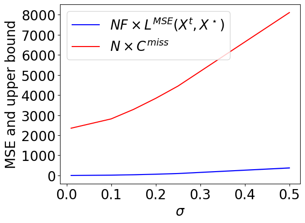
Figure 3: Emprical validation of Theorem 4.2 by comparing the value of the upper bound $N\times C^{\text{miss}}$ and $NF\times\mathcal{L}^{\text{MSE}}(X^{t},X^{\star})$ where $t$ is the final round for F3I. Left: MCAR setting. Center: MAR setting. Right: MNAR setting.

Table 3: Empirical validation of Theorem 4.2 by comparing the value of the upper bound $N\times C^{\text{miss}}$ and the average and standard deviation value of $NF\times\mathcal{L}^{\text{MSE}}(X^{t},X^{\star})$ across iterations where $t$ is the final round for F3I. All values are rounded to the closest second decimal place. Theorem 4.2 states that $\mathcal{L}^{\text{MSE}}(X^{t},X^{\star})\leq C^{\text{miss}}/F$ with probability $1-1/50$.

Missingness type	$\sigma$	$NF\times\mathcal{L}^{\text{MSE}}(X^{t},X^{\star})$	$N\times C^{\text{miss}}$
MCAR (Assumption 3.2)	0.01	0.63$\pm$ 0.38	2,352.60
	0.10	16.36$\pm$ 0.93	2,816.02
	0.15	36.12$\pm$ 1.89	3,286.57
	0.20	63.26$\pm$ 3.14	3,839.30
	0.25	97.44$\pm$ 4.56	4,450.16
	0.50	376.29$\pm$ 16.76	8,109.04
MAR (Assumption 3.3)	0.01	0.42$\pm$ 0.21	2,352.60
	0.10	11.53$\pm$ 0.78	2,816.02
	0.15	25.19$\pm$ 1.58	3,286.57
	0.20	44.07$\pm$ 2.65	3,839.30
	0.25	68.50$\pm$ 4.08	4,450.16
	0.50	266.19$\pm$ 15.22	8,109.04
MNAR (Assumption 3.4)	0.01	0.37$\pm$ 0.23	2,352.60
	0.10	7.13$\pm$ 0.64	2,816.02
	0.15	15.50$\pm$ 1.22	3,286.57
	0.20	26.53$\pm$ 1.86	3,839.30
	0.25	40.36$\pm$ 2.66	4,450.16
	0.50	152.03$\pm$ 9.56	8,109.04

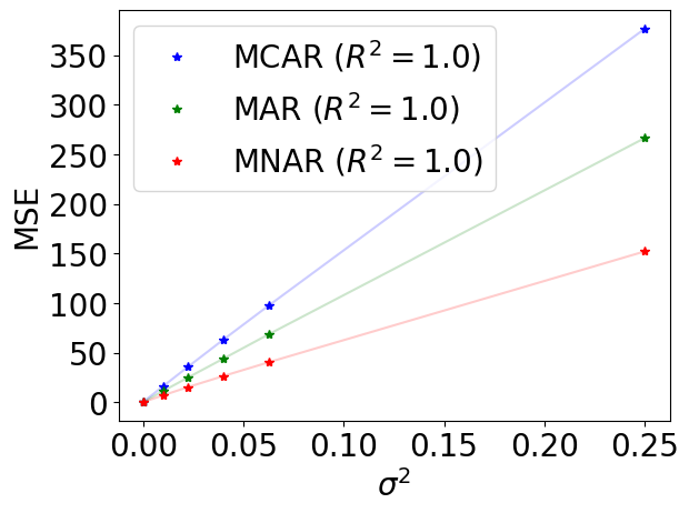
Figure 4: $NF\times\mathcal{L}^{\text{MSE}}(X^{t},X^{\star})$ is linear in $\sigma^{2}$ regardless of the missingness mechanism (numerical values are reported in Table 3).

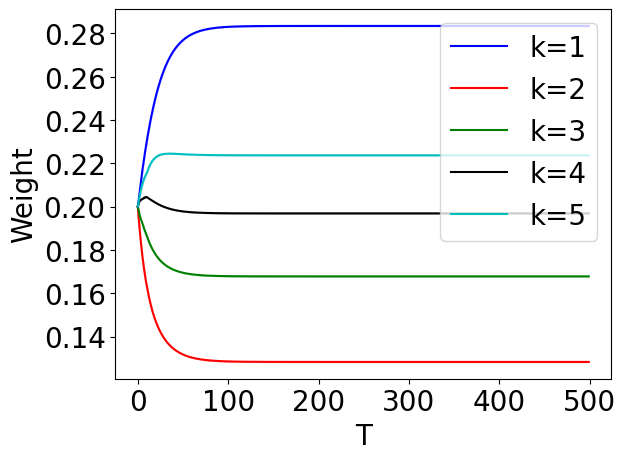
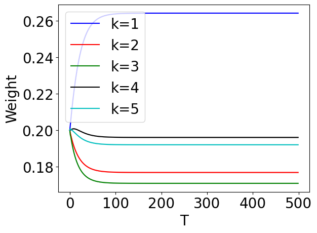
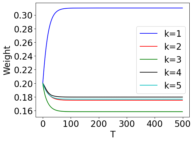
Figure 5: Evolution of the weight of each of the $K$-nearest neighbors for each sample as computed by F3I, where the $k$ neighbor is the $k^{\text{th}}$-nearest point, depending on the round $T$. Left: MCAR setting. Center: MAR setting. Right: MNAR setting.

Behavior of $\bm{\alpha}^{t}$ depending on imputation round $t$

Second, we look at the evolution of $\bm{\alpha}^{t}$ depending on the round $t$, knowing that at $t=0$, $\bm{\alpha}^{0}=\frac{1}{K}\bm{1}_{K}$ is a uniform weight vector. Figure 5 displays the evolution of weight $(\alpha^{t})_{k}$ for each $k$-nearest neighbor in iteration $t$ in F3I. Surprisingly enough, the optimal weight vector is not proportional to the rank of the neighbor; that is, the closer the neighbor, the higher the weight, which often motivates some heuristics about k-nearest neighbor algorithms. Optimality (preserving the data distribution) puts higher weights on the first and last closest neighbors.

Empirical validation of Theorem 4.5

Third, we look at the upper bound for the expected cumulative regret stated in Theorem 4.5. Using a missingness frequency of $25\%$ again, we run $100$ times F3I on synthetic data sets for all three missingness mechanisms and track the values of $\max_{\bm{\alpha}\in\triangle_{K}}\sum_{s=1}^{t}G_{*}(\bm{\alpha},X^{s-1})-G_{*}(\bm{\alpha}^{s},X^{s-1})$ and its upper bound $C^{\text{AH}}\sqrt{t}+H^{\text{miss}}h^{-1}t$ across iterations, where $t$ is the final step of F3I (that can change across iterations). We compute the value of $\max_{\bm{\alpha}\in\triangle_{K}}\sum_{s=1}^{t}G_{*}(\bm{\alpha},X^{s-1})$ by solving the related convex problem with function minimize in Python package scipy.optimize (Virtanen et al., 2020) after running F3I

$$\min_{\bm{\alpha}\in\mathbb{R}^{K}}-\sum_{s=1}^{t}G_{\star}(\bm{\alpha},X^{s-1})\quad\text{ such that }\quad\forall k\leq K,\ \alpha_{k}\geq 0\quad\text{ and }\quad\sum_{k\leq K}\alpha_{k}=1\;,$$

where $G_{\star}$ is computed with respect to the true complete points $\{(\bm{x}^{\star})_{1},\dots,(\bm{x}^{\star})_{N}\}$ and $(\bm{x}^{s})_{i}=\texttt{Impute}((\bm{x}^{s-1})_{i};\bm{\alpha}^{s})$ if $s\geq 1$ and $X^{0}$ is the naively imputed matrix. Figure 6 and Table 4 show that the upper bound is always valid across those experiments. Some random data sets among the 100 might be harder than the others, incurring larger regret. However, Figure 6 shows that the upper bound adapts to these instances. The large gap between the empirical and theoretical peaks in hardness might be due, as for Theorem 4.2, to the conservative estimates given by Bernstein’s inequality.

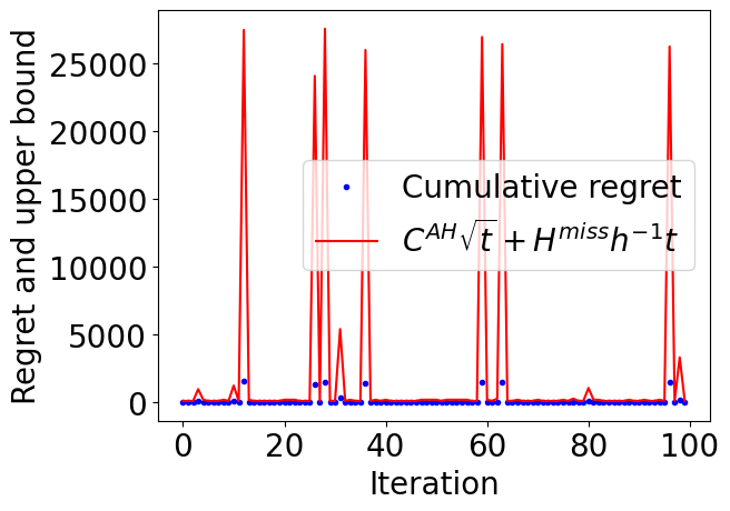
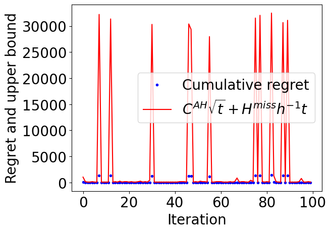
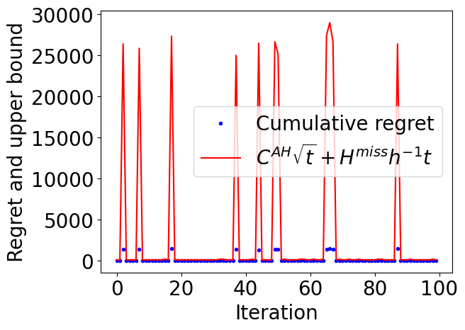
Figure 6: Cumulative regret for F3I and upper bound from Theorem 4.5 across $100$ iterations. The blue points are always below the red lines. Left: MCAR setting. Center: MAR setting. Right: MNAR setting.

Table 4: Empirical validation of Theorem 4.5 by comparing the value of the upper bound and the average and standard deviation value of the cumulative regret $\max_{\bm{\alpha}\in\triangle_{K}}\sum_{s=1}^{t}G_{*}(\bm{\alpha},X^{s-1})-G_{*}(\bm{\alpha}^{s},X^{s-1})$ across iterations where $t$ is the final round for F3I (the maximum number of rounds is set to $500$). All values are rounded to the closest second decimal place, except for the time round $t$, which is rounded to the closest integer. Theorem 4.5 states that $\max_{\bm{\alpha}\in\triangle_{K}}\sum_{s=1}^{t}G_{*}(\bm{\alpha},X^{s-1})-G_{*}(\bm{\alpha}^{s},X^{s-1})\leq C^{\text{AH}}\sqrt{t}+H^{\text{miss}}h^{-1}t$ with probability $1-1/2,500\approx 0.9996$.

Missingness type	$t$	Cumulative regret on $G$	$C_{G}^{\text{AH}}\sqrt{t}+H^{\text{miss}}h^{-1}t$
MCAR  (Assumption 3.2)	24$\pm$ 78	113.76$\pm$ 371.39	2,067.60$\pm$ 6,734.50
MAR    (Assumption 3.3)	40$\pm$ 111	153.06$\pm$ 417.40	3,542.96$\pm$ 9,659.89
MNAR  (Assumption 3.4)	35$\pm$ 96	158.61$\pm$ 438.45	3,015.86$\pm$ 8,336.243

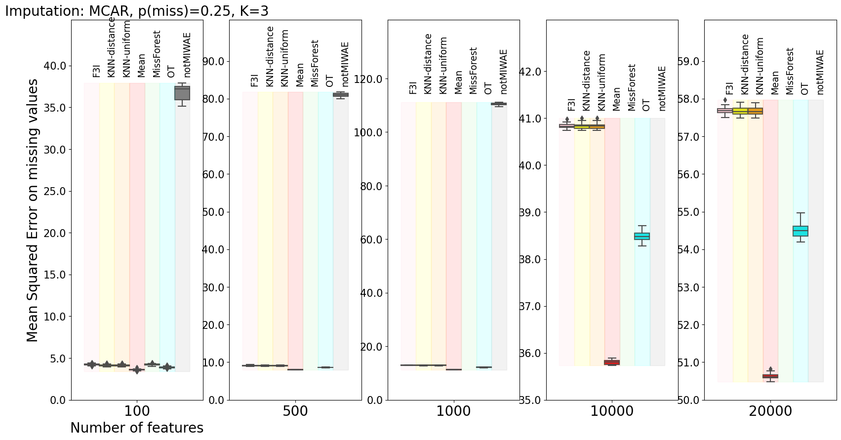
Figure 7: Imputation on $2$ synthetic data sets $\times$ $10$ different random seeds for generating missing values for F3I, K-nearest neighbor imputers (Troyanskaya et al., 2001) (uniform or distance-based weights), mean imputation, MissForest (Stekhoven & Bühlmann, 2012), Optimal-Transport imputer (Muzellec et al., 2020) and not-MIWAE (Ipsen et al., 2021).

F.1.2 Empirical performance (single imputation task)

Now we compare the MSE of F3I to its baselines on synthetic data sets generated with Algorithm 3. Note that the definition of the MSE is slightly different from Definition 4.1 as we only compute the gaps in the positions of missing values

$$\overline{\mathcal{L}}^{\text{MSE}}(X^{t},X^{\star})\triangleq\frac{1}{N}\sum_{i\leq N}\frac{1}{|\{f\mid m^{f}_{i}=1\}|}\sum_{f,m^{f}_{i}=1}((x^{t})^{f}_{i}-(x^{\star})^{f}_{i})^{2}\leq F\mathcal{L}^{\text{MSE}}(X^{t},X^{\star})\;.$$

We consider the following baselines: imputation by the mean value, random-forest-based imputation by MissForest (Stekhoven & Bühlmann, 2012), traditional KNN imputation (Troyanskaya et al., 2001) with uniform and distance-based weights, Optimal Transport-based imputation (Muzellec et al., 2020) and the Bayesian network approach not-MIWAE (Ipsen et al., 2021). We consider a number of neighbors (for F3I and KNN) or of estimators (for MissForest) $K=3$, a number of features $F\in\{100;500;1,000;10,000;20,000\}$ with $N=50$ samples, and a missingness frequency $p^{\text{miss}}\propto\{0.10,0.25,0.50,0.75\}$. We generate $2$ random data sets and perform $10$ iterations of each algorithm on each data set, for a total of $20$ values per combination of parameters ($F$, missingness mechanism), where the missingness mechanism is either MCAR, MAR, or MNAR.

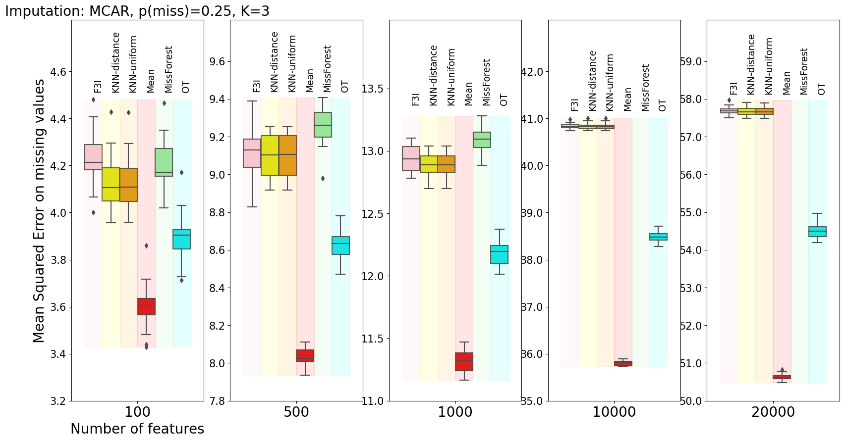
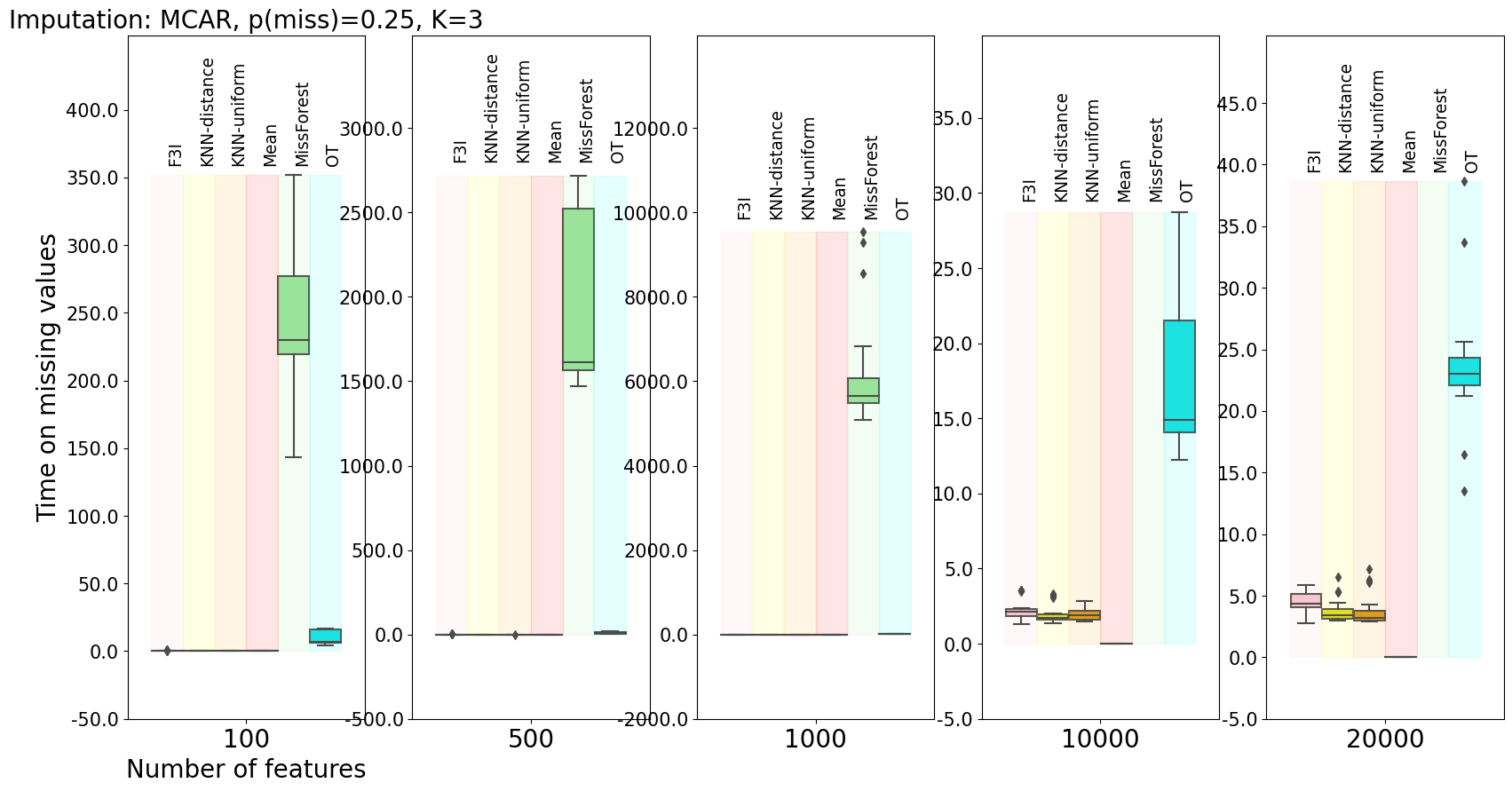
Figure 13: Imputation on $2$ synthetic data sets $\times$ $10$ different random seeds for generating missing values for F3I, K-nearest neighbor imputers (Troyanskaya et al., 2001) (uniform or distance-based weights), mean imputation, MissForest (Stekhoven & Bühlmann, 2012) and Optimal-Transport imputer (Muzellec et al., 2020).

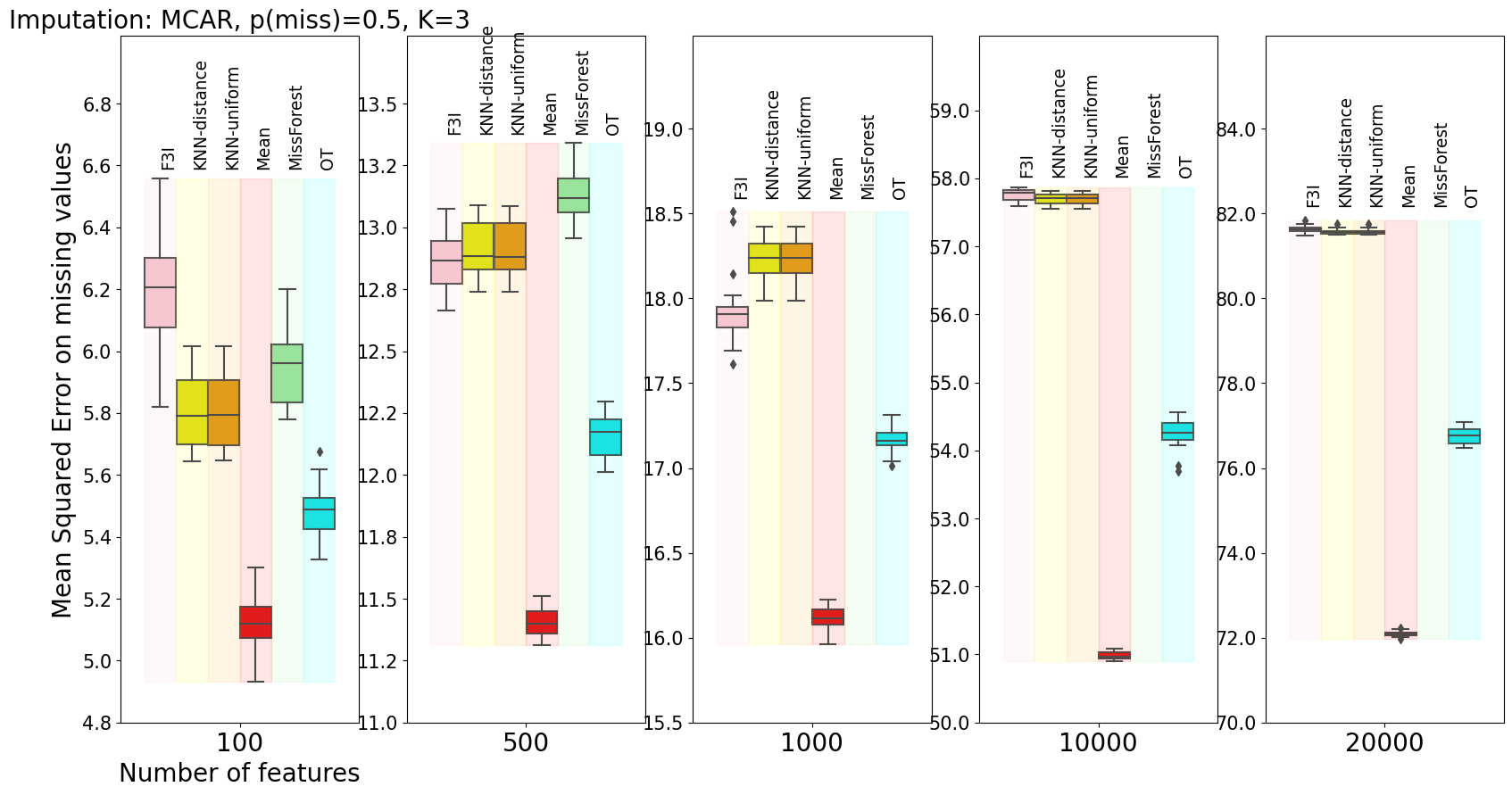
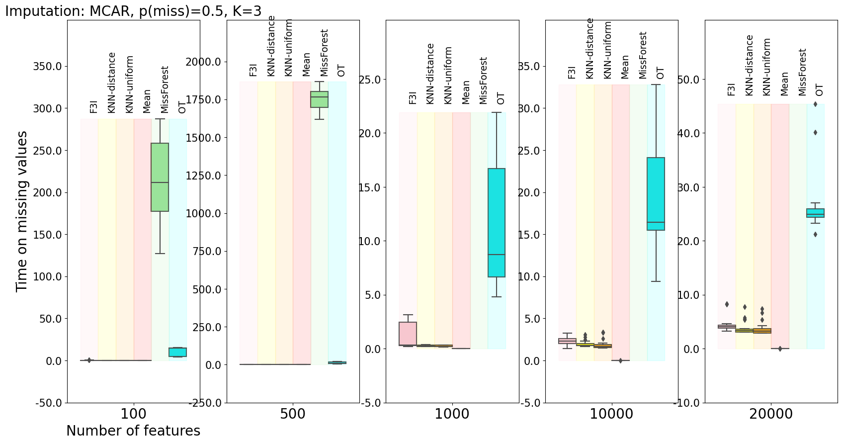
Figure 14: Imputation on $2$ synthetic data sets $\times$ $10$ different random seeds for generating missing values for F3I, K-nearest neighbor imputers (Troyanskaya et al., 2001) (uniform or distance-based weights), mean imputation, MissForest (Stekhoven & Bühlmann, 2012) and Optimal-Transport imputer (Muzellec et al., 2020).

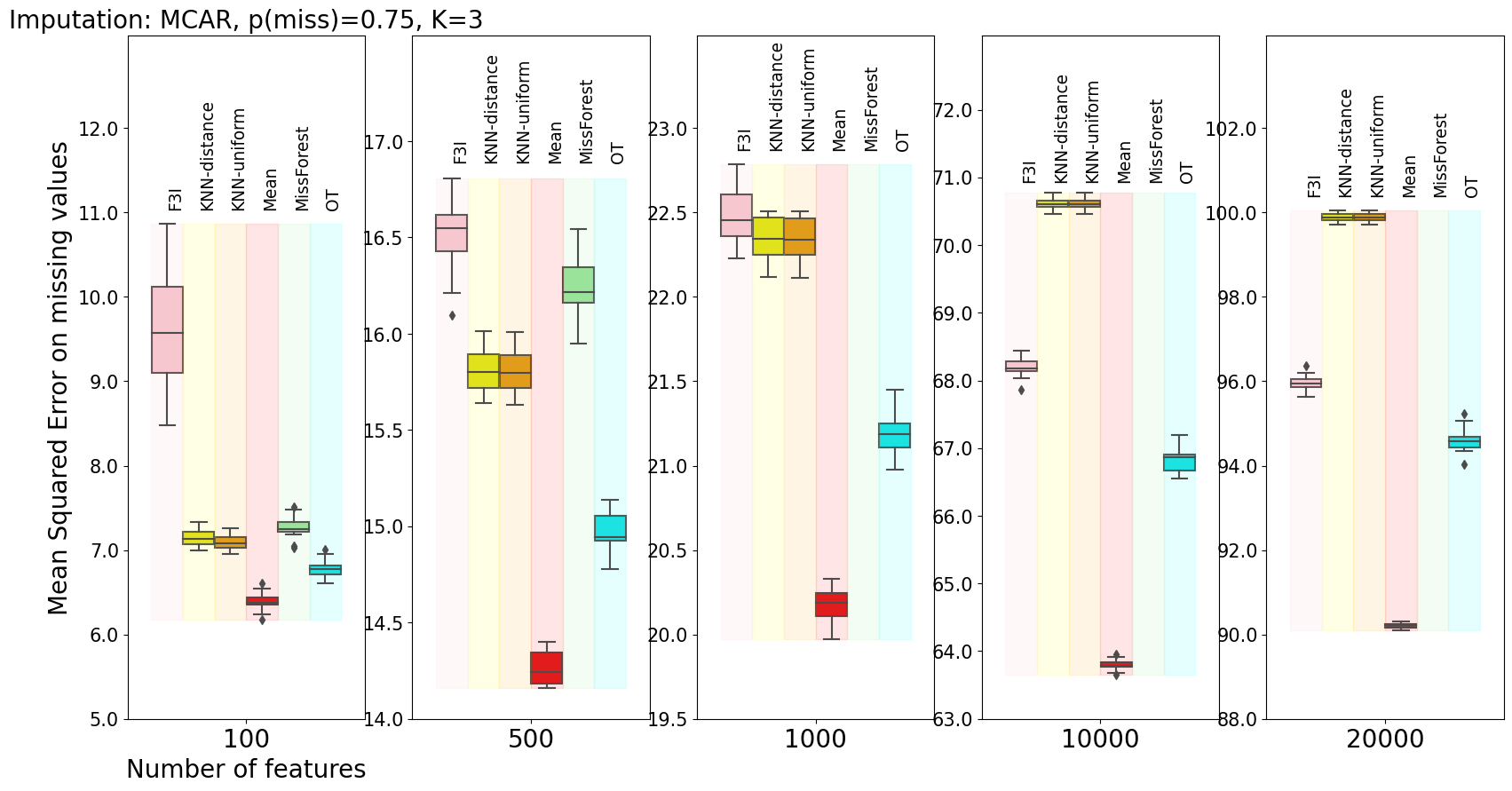
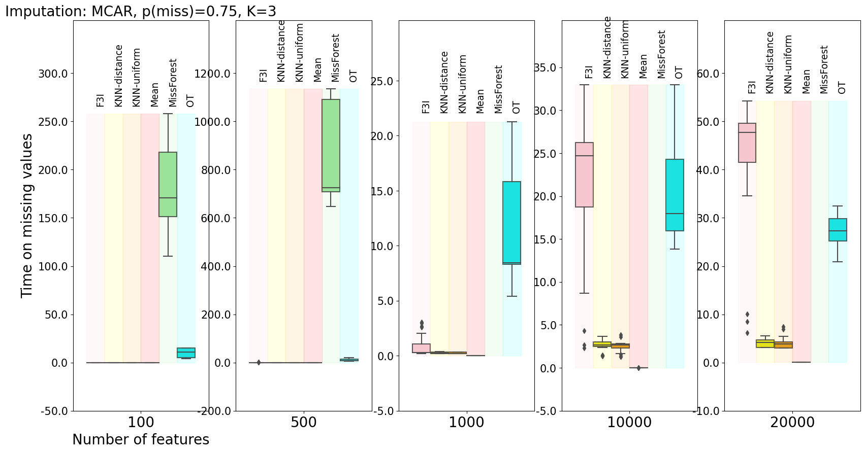
Figure 15: Imputation on $2$ synthetic data sets $\times$ $10$ different random seeds for generating missing values for F3I, K-nearest neighbor imputers (Troyanskaya et al., 2001) (uniform or distance-based weights), mean imputation, MissForest (Stekhoven & Bühlmann, 2012) and Optimal-Transport imputer (Muzellec et al., 2020).

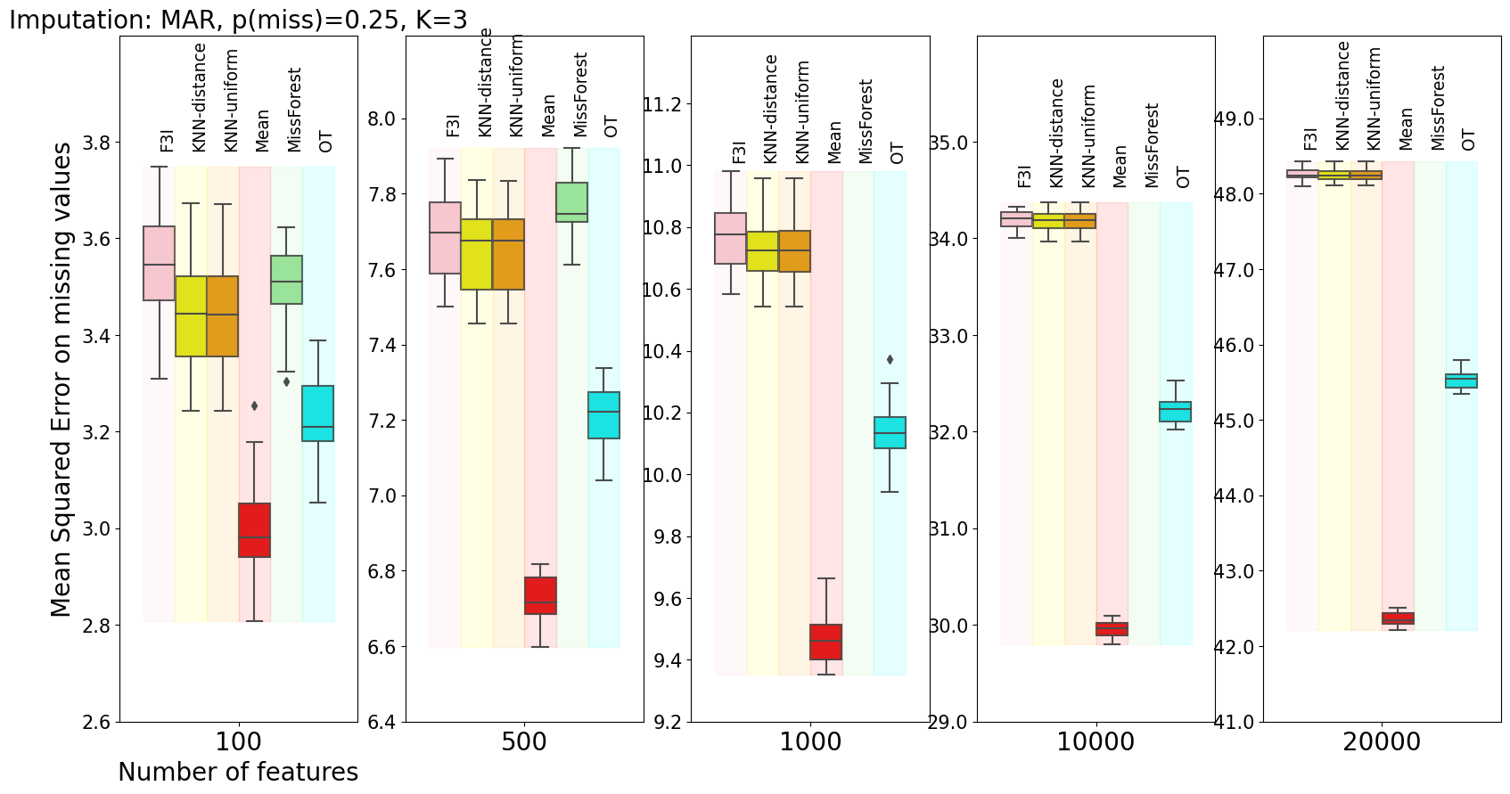
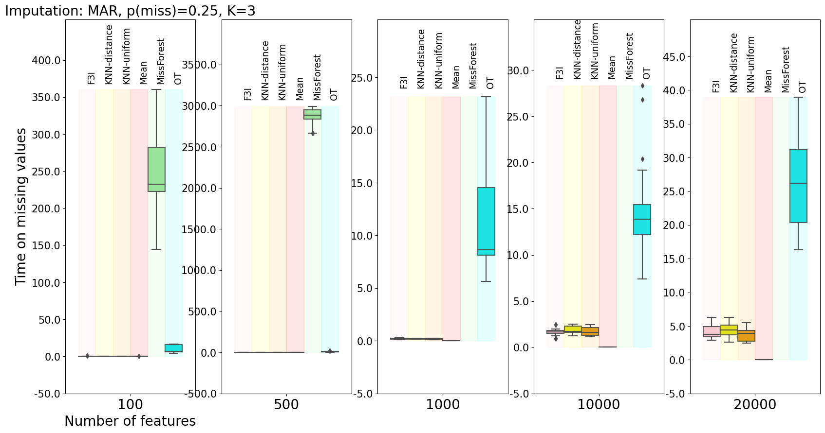
Figure 16: Imputation on $2$ synthetic data sets $\times$ $10$ different random seeds for generating missing values for F3I, K-nearest neighbor imputers (Troyanskaya et al., 2001) (uniform or distance-based weights), mean imputation, MissForest (Stekhoven & Bühlmann, 2012) and Optimal-Transport imputer (Muzellec et al., 2020).

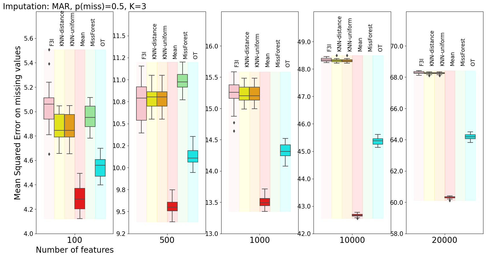
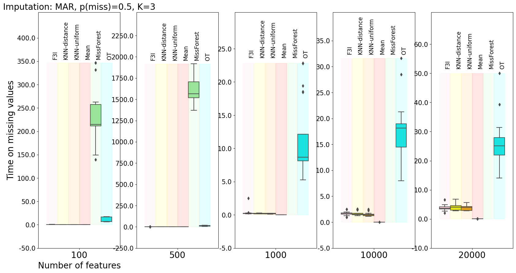
Figure 17: Imputation on $2$ synthetic data sets $\times$ $10$ different random seeds for generating missing values for F3I, K-nearest neighbor imputers (Troyanskaya et al., 2001) (uniform or distance-based weights), mean imputation, MissForest (Stekhoven & Bühlmann, 2012) and Optimal-Transport imputer (Muzellec et al., 2020).

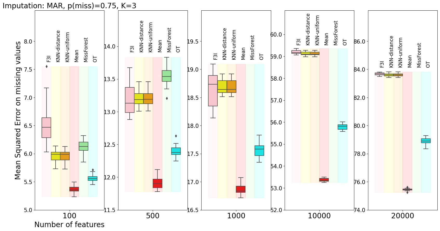
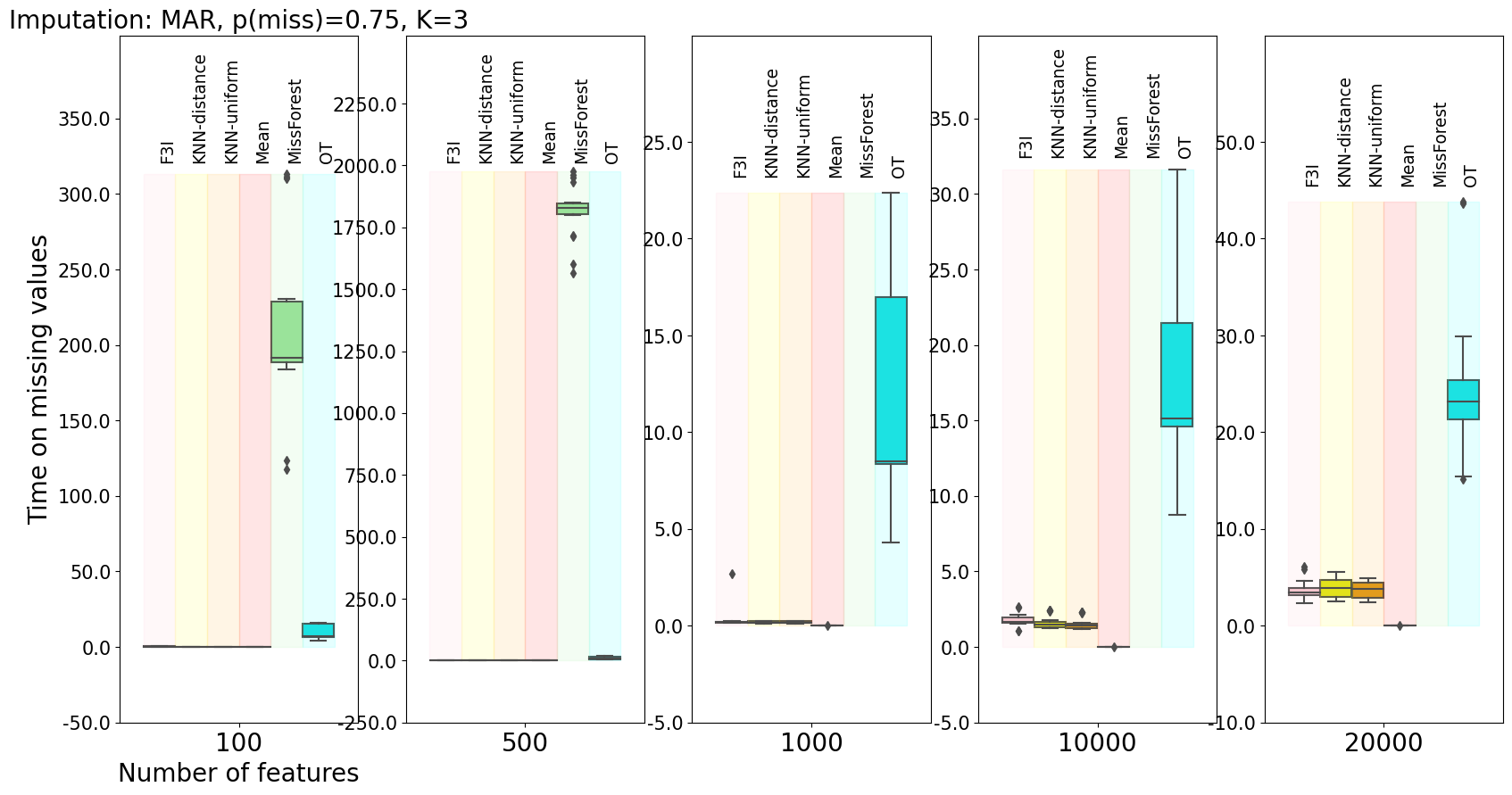
Figure 18: Imputation on $2$ synthetic data sets $\times$ $10$ different random seeds for generating missing values for F3I, K-nearest neighbor imputers (Troyanskaya et al., 2001) (uniform or distance-based weights), mean imputation, MissForest (Stekhoven & Bühlmann, 2012) and Optimal-Transport imputer (Muzellec et al., 2020).

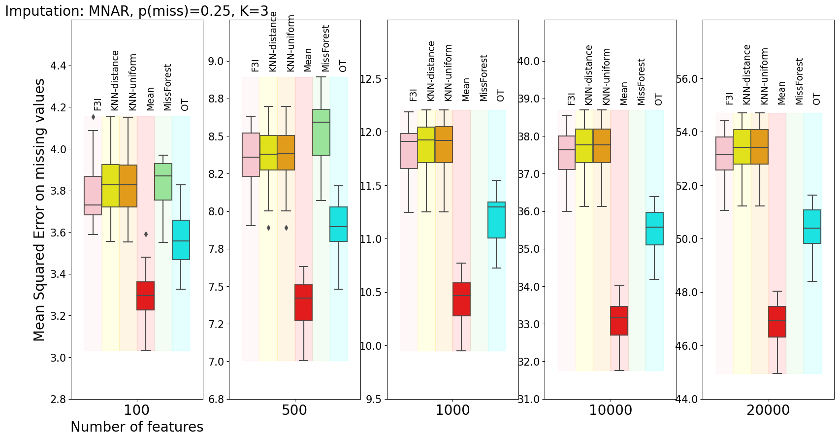
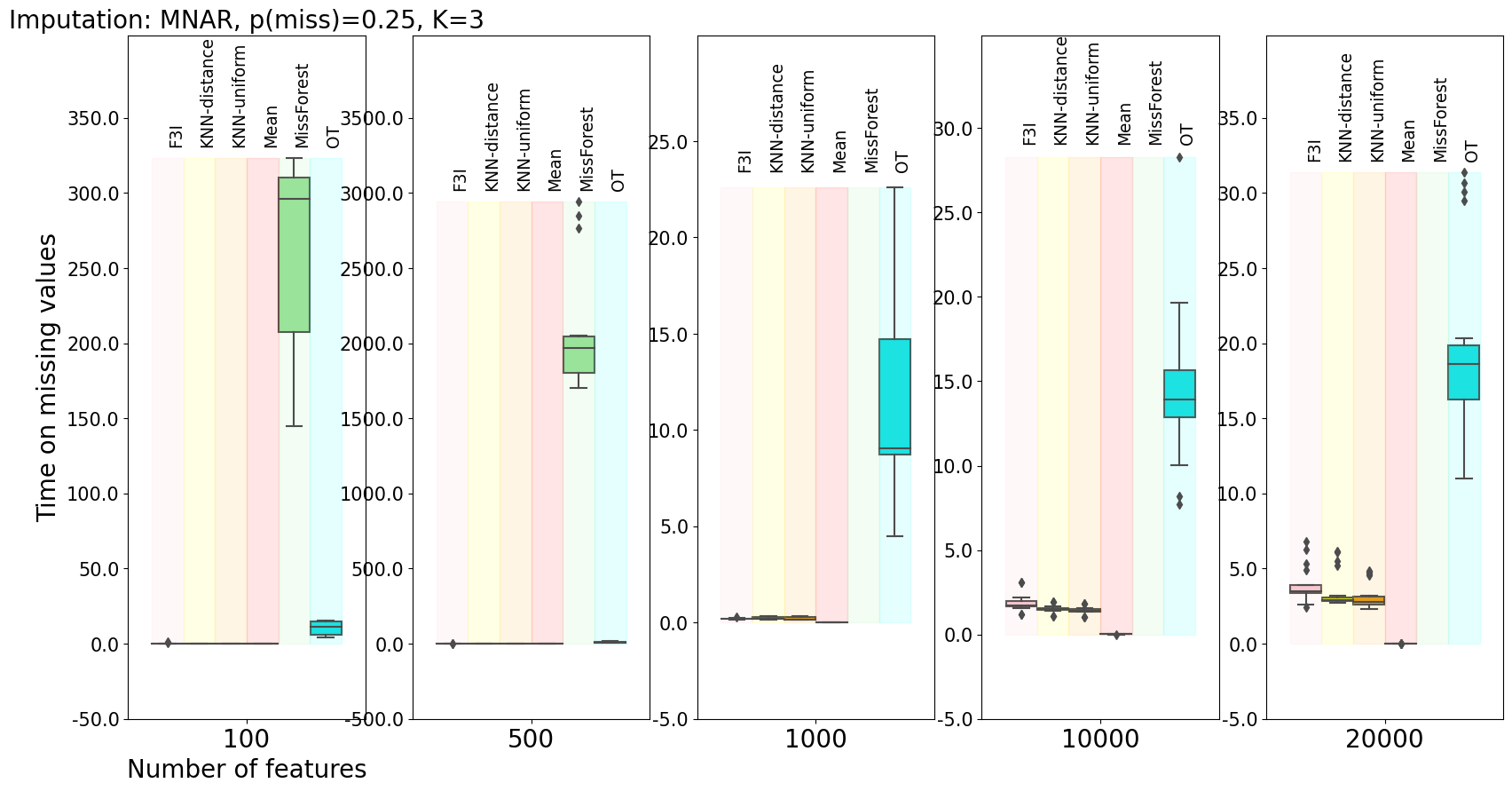
Figure 19: Imputation on $2$ synthetic data sets $\times$ $10$ different random seeds for generating missing values for F3I, K-nearest neighbor imputers (Troyanskaya et al., 2001) (uniform or distance-based weights), mean imputation, MissForest (Stekhoven & Bühlmann, 2012) and Optimal-Transport imputer (Muzellec et al., 2020).

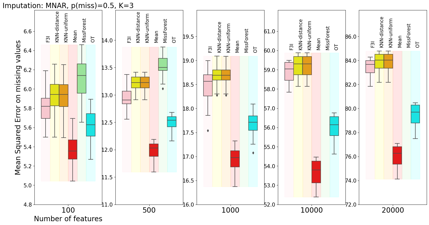
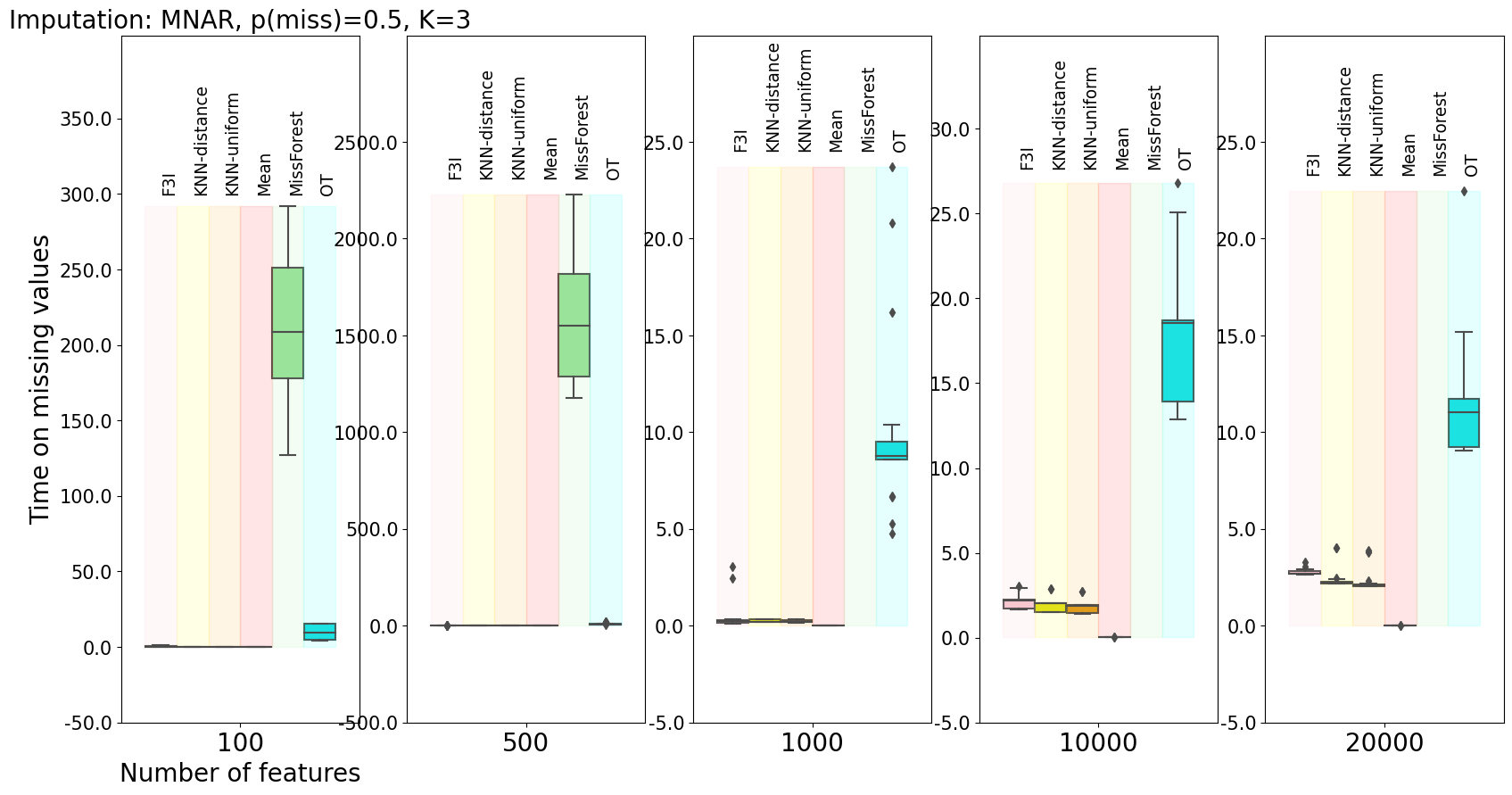
Figure 20: Imputation on $2$ synthetic data sets $\times$ $10$ different random seeds for generating missing values for F3I, K-nearest neighbor imputers (Troyanskaya et al., 2001) (uniform or distance-based weights), mean imputation, MissForest (Stekhoven & Bühlmann, 2012) and Optimal-Transport imputer (Muzellec et al., 2020).

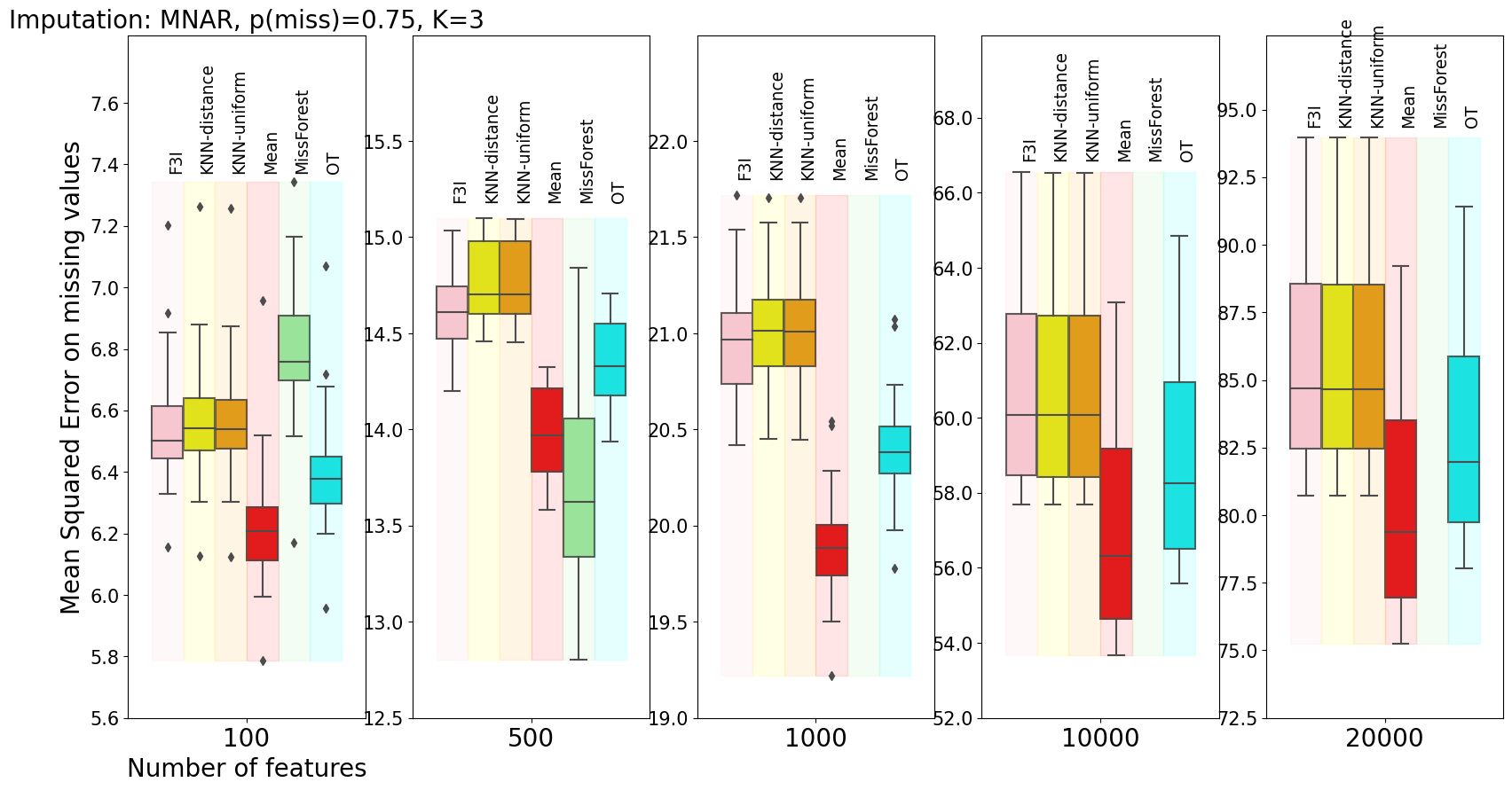
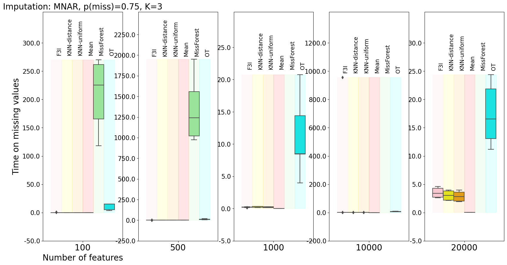
Figure 21: Imputation on $2$ synthetic data sets $\times$ $10$ different random seeds for generating missing values for F3I, K-nearest neighbor imputers (Troyanskaya et al., 2001) (uniform or distance-based weights), mean imputation, MissForest (Stekhoven & Bühlmann, 2012) and Optimal-Transport imputer (Muzellec et al., 2020).

We first note that not-MIWAE has a significantly worse imputation error than all other algorithms; see Figure 7. We then do not report the results for not-MIWAE in all other cases. Moreover, from $F=1,000$, the runtime of MissForest is too long to be run. The remainder of the boxplots for the mean squared error and imputation runtime across iterations and data sets can be found in Figures 13-21.

Second, we note the superior performance of F3I, nearest neighbor, and mean imputers regarding the computational cost of imputation across missingness frequencies $p^{\text{miss}}$, missingness mechanisms (MCAR, MAR, MNAR), and numbers $F$ of features. This makes F3I a competitive approach when the number of features is huge (for instance, $F\in\{10,000;20,000\}$).

Third, as a general rule across missingness mechanisms and frequencies, the performance of F3I is close to the ones of other nearest-neighbor imputers and sometimes better when the number of features is large. It might be because F3I considers the same neighbors across features past the initial imputation step. This allows us to impute perhaps more reliably missing values, contrary to the other NN imputers where neighbor assignation is performed feature-wise. Moreover, we notice that the performance of F3I and all baselines are on par (that is, boxplots overlap) for data where the missing values are generated from a MNAR mechanism (Figures 19-21) regardless of the missing frequency.

Fourth, F3I performs worst for data generated by a MCAR or a MAR mechanism, which is the setting where mean imputation works best. This might make sense, as F3I tries to capture a specific missingness pattern that depends on neighbors in the data set. The (perfectly) random pattern might be the most difficult to infer for F3I and other nearest-neighbor imputers.

F.1.3 Validation of theoretical results (joint imputation-classification task)

We implement the joint imputation-classification training with the log-loss function and sigmoid classifier $\ell(\bm{x})\triangleq-y\log C_{\bm{\omega}}(\bm{x})$ mentioned in Example 1 (Appendix D), where $y\in\{0,1\}$ is the binary class associated with sample $\bm{x}\in\mathbb{R}^{F}$. To implement PCGrad-F3I, we chain the imputation phase by F3I with an MLP, which returns logits. At time $t$, the imputation part applies at a fixed set of parameters $\bm{\omega}^{t}$ with the learner losses defined in Equation (2). We construct the synthetic data sets for classification as follows. We draw two random matrices in the synthetic data set as in Algorithm 3 corresponding to the item and user feature matrices. We assign binary class labels to each item-user pair using a K-means++ algorithm (Arthur & Vassilvitskii, 2006) with $K=2$ clusters on the item-user concatenated feature vectors.

We first validate the upper bound on the cumulative regret in Theorem 5.1 for all three missingness mechanisms we studied, similar to what was done for Theorem 4.5. As in our proofs (see Appendix D), we consider the log-loss $\ell$ with the sigmoid classifier $C_{\bm{\omega}}$ and $\beta=0.5$. We consider a missingness frequency of $50\%$. To obtain the value of $\arg\,\max_{\bm{\alpha}\in\triangle_{K}}\sum_{s=1}^{t}\overline{G}(\bm{\alpha},X^{s-1})$, where $\overline{G}$ is defined as

$$\overline{G}:\bm{\alpha}\in\triangle_{K},X\in\mathbb{R}^{N\times F}\mapsto(1-\beta)G_{\star}(\bm{\alpha},X)-\frac{\beta}{N}\sum_{i\leq N}\ell(\bm{x}_{i}(\bm{\alpha}))\;,$$

we solve the following optimization problem by solving the related convex problem with function minimize in Python package scipy.optimize (Virtanen et al., 2020), considering the $(X^{s-1})_{s\leq t}$ and parameter of the sigmoid classifier $C_{\omega}$ in the last epoch in PCGrad-F3I

$$\min_{\bm{\alpha}\in\mathbb{R}^{K}}-\sum_{s=1}^{t}\overline{G}(\bm{\alpha},X^{s-1})\quad\text{ such that }\quad\forall k\leq K,\ \alpha_{k}\geq 0\quad\text{ and }\quad\sum_{k\leq K}\alpha_{k}=1\;.$$

The gradient and the Hessian matrix of the objective function $\overline{G}$ with respect to $\bm{\alpha}$ are obtained by combining the results from Lemmas A.3, Lemma A.4 and Section D. Figure 8 and Table 5 indeed show that the upper bound reliably holds on the cumulative regret for $\overline{G}$.

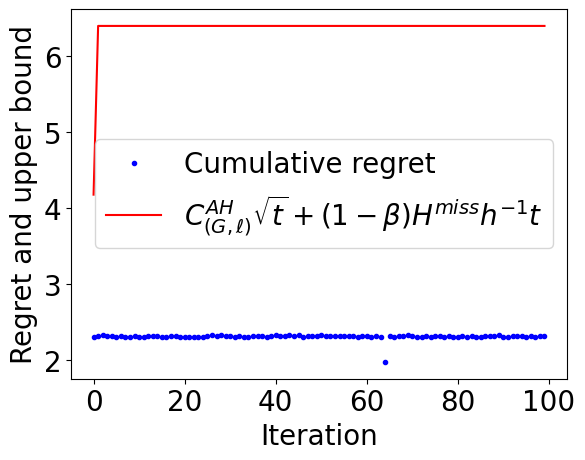
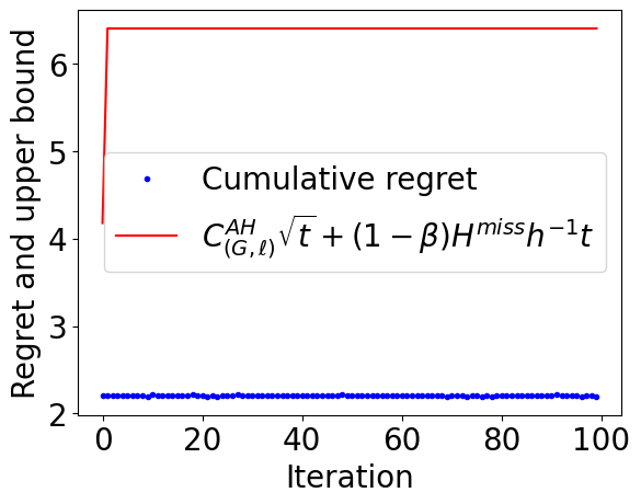
Figure 8: Cumulative regret for F3I and upper bound from Theorem 5.1 across $100$ iterations for $\beta=0.5$. The blue points are always below the red lines. Left: MCAR setting. Center: MAR setting. Right: MNAR setting.

Table 5: Empirical validation of Theorem 5.1 by comparing the value of the upper bound and the average and standard deviation value of the cumulative regret $\max_{\bm{\alpha}\in\triangle_{K}}\sum_{s=1}^{t}\overline{G}(\bm{\alpha},X^{s-1})-\overline{G}(\bm{\alpha}^{s},X^{s-1})$ across iterations where $t$ is the final round for F3I in the last epoch. All values are rounded to the closest second decimal place. The time round is fixed to $T=3$ in PCGrad-F3I and $\beta=0.5$. Theorem 4.5 states that $\max_{\bm{\alpha}\in\triangle_{K}}\sum_{s=1}^{t}\overline{G}(\bm{\alpha},X^{s-1})-\overline{G}(\bm{\alpha}^{s},X^{s-1})\leq C^{\text{AH}}_{(G,\ell)}\sqrt{t}+(1-\beta)H^{\text{miss}}h^{-1}t$ with probability $1-1/2,500\approx 0.9996$.

Missingness type	$t$	Cumulative regret on $\overline{G}$	$C_{(G,\ell)}^{\text{AH}}\sqrt{t}+(1-\beta)H^{\text{miss}}h^{-1}t$
MCAR  (Assumption 3.2)	3	2.31 $\pm$0.03	6.38 $\pm$0.22
MAR    (Assumption 3.3)	3	2.21 $\pm$0.01	6.37 $\pm$0.22
MNAR  (Assumption 3.4)	3	2.21 $\pm$0.00	6.38 $\pm$0.22

F.1.4 Empirical performance (joint imputation-classification task)

Then, we compare the performance of PCGrad-F3I with adding a NeuMiss block (Le Morvan et al., 2020) and with performing an imputation by the mean (“Mean”) before the classifier. Similarly to PCGrad-F3I, we chain an imputation part with an MLP classifier, which returns logits. In the baselines, at time $t$, the imputation part applies at a fixed set of parameters $\bm{\omega}^{t}$ an imputation by the mean, or a shared-weights NeuMiss block, as introduced in Le Morvan et al. (2021). The criterion for training the model is the log loss, and we split the samples into training ($70\%$), validation ($20\%$), and testing ($10\%$) sets, where the former two sets are used for training the MLP, and the performance metrics are computed on the latter set. We consider the classical Area Under the Curve (AUC) on the test set (hidden during training) as the performance metric for the binary classification task. In this section, we set the number of imputation rounds in F3I to $T=2$, and we train the MLPs for each imputation approach with the hyperparameter values reported in Table 6.

Figure 9 shows the results for MCAR (Assumption 3.2), MAR (Assumption 3.3), and MCAR (Assumption 3.4) synthetic data with an approximate missingness frequency of $50\%$ and varying values of $\beta\in\{0.25,0.5,0.75\}$. Figure 10 shows the corresponding results when the approximated missingness frequency is in $\{25\%,75\%\}$. There is a significant improvement in PCGrad-F3I over the baseline NeuMiss. However, the imputation by the mean remains the top contender on the synthetic Gaussian data sets, as already noticed for imputation in the previous paragraph, even if PCGrad-F3I is sometimes on par regarding classification performance.

Table 6: Hyperparameter values for the training of the MLP block for each imputation method (NeuMiss, mean imputation, F3I).

Hyperparameter	Number of epochs	Weight decay in the optimizer	Learning rate	MLP depth
Value	10	0	0.01	1 layer

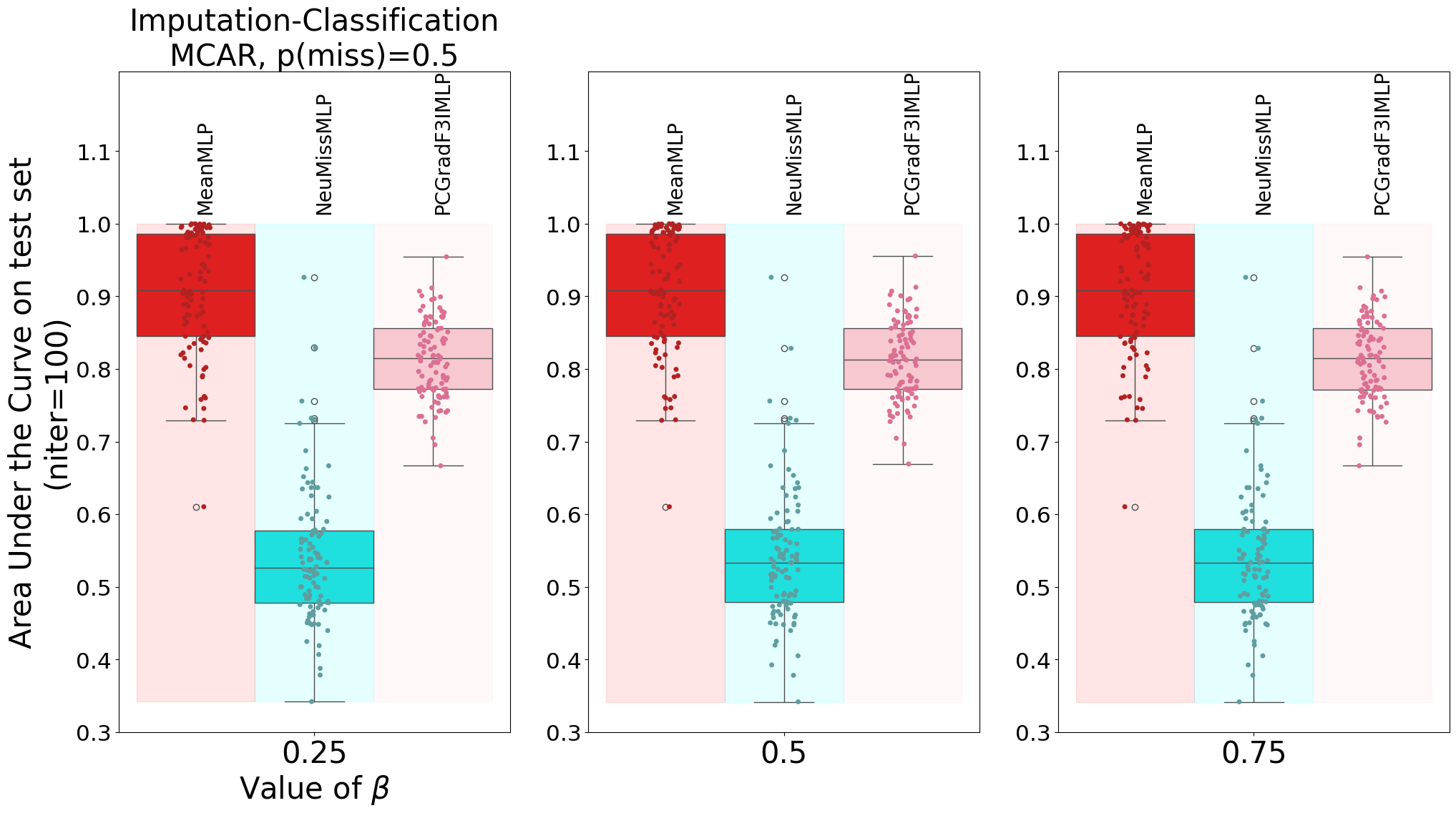
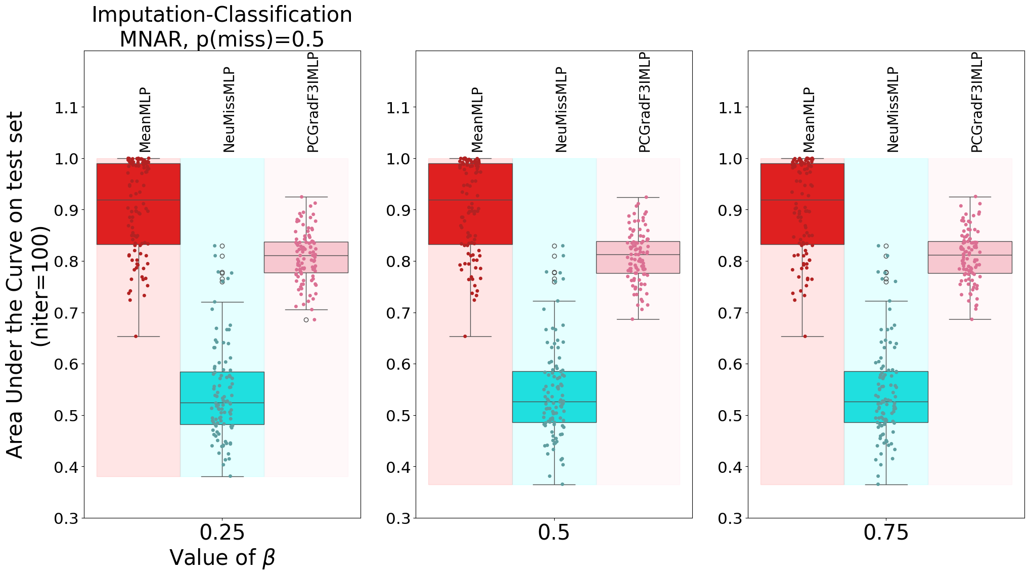
Figure 9: Joint-Imputation on a synthetic data set with MCAR (left), MAR (center) and MNAR (right) missing values and approximate missingness frequency $p^{\text{miss}}=0.5$, for $\beta\in\{0.25,0.5,0.75\}$.

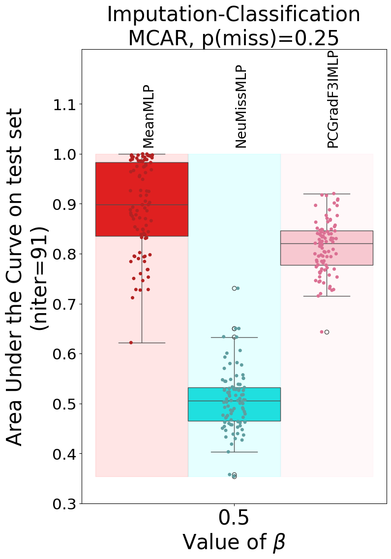
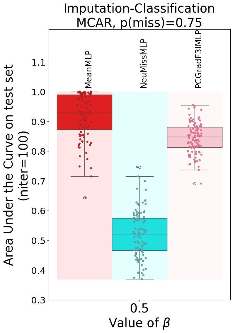
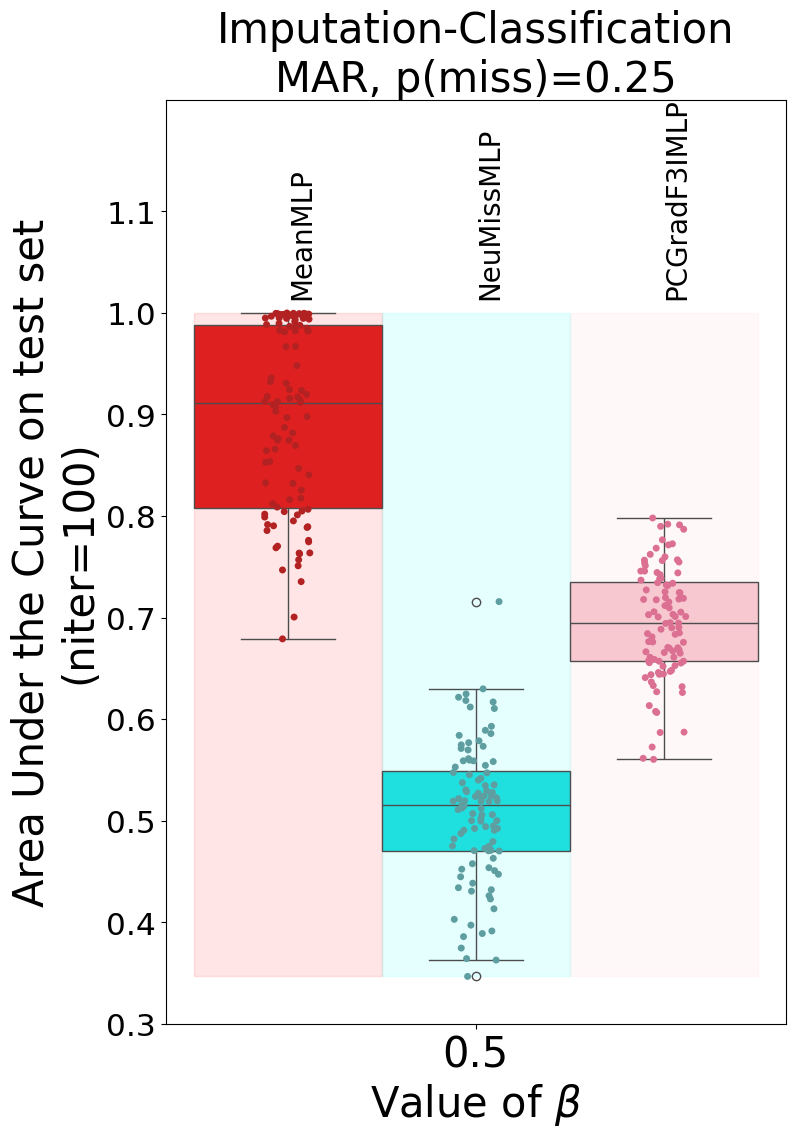
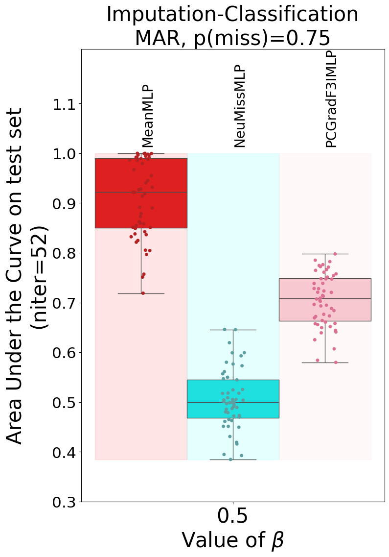
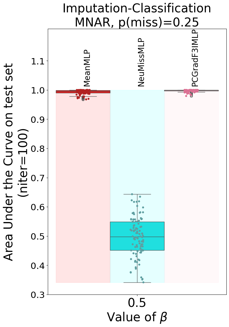
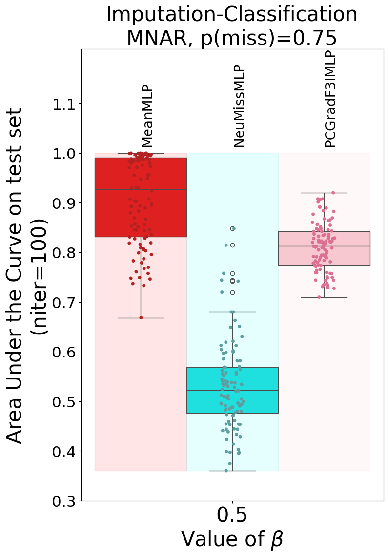
Figure 10: Joint-Imputation on a synthetic data set with MCAR (left), MAR (center) and MNAR (right) missing values and approximate missingness frequency $p^{\text{miss}}\in\{0.25,0.75\}$, for $\beta\in\{0.25,0.5,0.75\}$.

F.2 Real-life data sets (drug repurposing & handritten-digit recognition)

In addition to the synthetic Gaussian data sets, we also evaluate the performance of F3I on real-life data for drug repurposing or handwritten-digit recognition on the well-known MNIST data set (LeCun et al., 1998).

Drug repurposing aims to pair diseases and drugs based on their chemical, biological, and physical features. However, those features might be missing due to the incompleteness of medical databases or to a lack or failure of measurement. Table 7 reports the sizes of the considered drug repurposing data sets, which can be found online as indicated in their corresponding papers. A positive drug-disease pair is a therapeutic association (that is, the drug is known to treat the disease). In contrast, a negative one is associated with a failure in treating the disease or the emergence of toxic side effects.

Table 7: Overview of the drug repurposing data sets in the experimental study in Section F, with the number of drugs, drug features, diseases, disease features, along with the number of positive and negative drug-disease pairs.

Name of the data set	$N_{\text{drugs}}$       $F_{\text{drugs}}$	$N_{\text{diseases}}$       $F_{\text{users}}$	Positive pairs	Negative pairs
Cdataset (Luo et al., 2016)	663       663	409       409	2,532	0
DNdataset (Gao et al., 2022)	550    1,490	360    4,516	1,008	0
Gottlieb (Luo et al., 2016)	593       593	313       313	1,933	0
PREDICT-Gottlieb (Gao et al., 2022)	593    1,779	313       313	1,933	0
TRANSCRIPT (Réda, 2023b)	204  12,096	116  12,096	401	11

F.2.1 Imputation quality and runtimes (drug repurposing task)

First, we run $100$ times (with different random seeds) F3I and its baselines on each drug repurposing data set that comprises two feature matrices, one for drugs and another for diseases. We consider the K-nearest neighbor imputer with distance-associated weights, as they are often as performant in practice as uniform ones as seen above. Those data sets do not have any missing values, so we add missing values by a Gaussian self-masking mechanism (Le Morvan et al., 2020), for a missingness frequency approximately equal to $60\%$. The positions of missing values are the same across runs. Since the number of features $F\approx 12,000$ in the TRANSCRIPT dataset (Réda, 2023b) is prohibitive for most of the baselines, we reduce the number of features to $9,000$, selecting the features with the highest variance across drugs and diseases. Moreover, MissForest (Stekhoven & Bühlmann, 2012) and not-MIWAE (Ipsen et al., 2021) are too resource-consuming to be run on the largest data sets, DNdataset (Gao et al., 2022), PREDICT-Gottlieb (Gao et al., 2022) and TRANSCRIPT (Réda, 2023b). Figures 22-26 show the boxplots of average mean squared errors and runtimes of each algorithm across the $100$ iterations for both drug and disease feature matrices.

Overall, F3I has a runtime comparable to the fastest baselines, that is, the Optimal Transport-based imputer (Muzellec et al., 2020) (OT in plots), the imputation by the mean value (Mean) and the k-nearest neighbor approach (Troyanskaya et al., 2001) (KNN), while having a performance in imputation which is on par with the best state-of-the-art algorithm MissForest (Stekhoven & Bühlmann, 2012), as reported by several prior works (Emmanuel et al., 2021; Joel et al., 2024). However, MissForest is several orders of magnitude slower than F3I and sometimes cannot be run at all (for instance, for the highly-dimensional TRANSCRIPT data set). The Optimal Transport imputer also performs well across the data sets and often competes with our contribution F3I in imputation and computational efficiency.

F.2.2 Classification quality (handwritten-digit recognition task)

Again, we compare the performance of PCGrad-F3I with a simple mean imputation or NeuMiss (Le Morvan et al., 2020, 2021), chaining the corresponding imputation part with an MLP as previously done on synthetic data sets in Subsection F.1. We consider the MNIST dataset (LeCun et al., 1998), which comprises grayscale images of $25\times 25$ pixels. We restrict our study to images annotated with class 0 or class 1 to get a binary classification problem. We remove pixels at random with probability 50% using a MCAR mechanism (Assumption 3.2).

Table 8: Fine-tuned hyperparameter values using Optuna to train the MLP block for each imputation method (NeuMiss, Mean imputation, PCGradF3I) on the MNIST data set. K, T, $\beta$ and $\eta$ are F3I-specific parameters, whereas all remaining parameters are common to all three methods and belong to the MLP block.

Hyperparameter	Number of epochs	Learning rate	MLP depth	K	T	$\beta$	$\eta$
Value	10	0.01	5 layers	19	30	0.142	0.023

Table 9: Area Under the Curve (AUC) values (average $\pm$ standard deviation) in the testing subset in MNIST (hidden during the training phase) and corresponding tuned hyperparameter values (rounded up to the $3^{\text{rd}}$ decimal place for values in $\mathbb{R}$) for $N=100$ iterations. NeuMiss has been trained on the same number of epochs and the same MLP architecture as PCGradF3I and the mean imputation followed by the MLP (Mean imputation). Those are the same results displayed in Table 1.

Type	$p^{\text{miss}}$	Algorithm	AUC
MCAR (Assumption 3.2)	$50\%$	Mean imputation	0.640 $\pm$0.180
		NeuMiss (Le Morvan et al., 2020)	0.989 $\pm$0.069
		PCGradF3I (ours)	0.990 $\pm$0.094

Hyperparameter tuning. We employed the Optuna framework to optimize our model’s hyperparameters (Akiba et al., 2019). The optimization process focused on tuning several key parameters: $\beta,\eta,T,K$, and the depth of the classifier MLP. For the hyperparameter search, we utilized Optuna’s default Tree-structured Parzen Estimator-based sampler (Bergstra et al., 2011), conducting 50 trials to explore the parameter space. The dataset was evenly divided into three portions, with 34% allocated for training, 33% for validation, and 33% for testing. During the optimization process, we aimed to maximize the logarithm of the Area Under the Curve (AUC) scores from the Receiver Operating Characteristic (ROC) curve on the validation set. After identifying the optimal hyperparameter configuration, we constructed the final model. Final hyperparameter values are reported in Table 8.

Training. This optimized model underwent training using the designated training set, followed by performance evaluation. We assessed its performance by measuring the AUC score of the ROC curve on the test set, repeating this evaluation process across 100 iterations to ensure robust results.

Results. We report the numerical results in Table 9. We also display the imputed images for the first $6$ samples in MNIST by F3I or by mean imputation,  trained on the first 600 samples. We vary $p^{\text{miss}}\in\{25\%,50\%,75\%\}$ in Figure 11. Finally, we modify the missingness mechanism in Figure 12, switching the MCAR missingness mechanism to MAR (Assumption 3.3) or MNAR (Assumption 3.4).

As mentioned in the main text, PCGradF3I beats the mean imputation and NeuMiss regarding classification accuracy according to Table 9. It also preserves a good imputation of the MNIST images compared to the mean imputation, even when the number of missing values increases (see Figure 11). Even if one still can distinguish between ones and zeroes with the mean imputation, there is a higher confidence in the predicted labels when looking at F3I-imputed images. Moreover, F3I turns out to be more robust to the different types of missingness mechanisms compared to the mean imputation, as illustrated by Figure 12. For missing-completely-at-random pixels, both methods fare good regarding imputation. However, the performance of the mean imputation is limited in the case of MAR or MNAR-missing pixels (Columns 4 et 6), as most samples represent both a 0 and a 1.

Figure 11: Imputed grayscale images by F3I (first two rows) or mean imputation (last two rows) for the first $6$ samples (trained on the first 600 samples of MNIST with the hyperparameters in Table 8) with MCAR-missing pixels, with missingness frequencies in $\{25\%,50\%,75\%\}$. Columns 1 to 3 correspond to $p^{\text{miss}}=25\%$, columns 4 to 6 to $p^{\text{miss}}=50\%$, and columns 7 to 9 to $p^{\text{miss}}=75\%$. Positions of red pixels represent missing pixels during the training phase which are imputed by either F3I or mean imputation (same figure as Figure 2 in the main text).

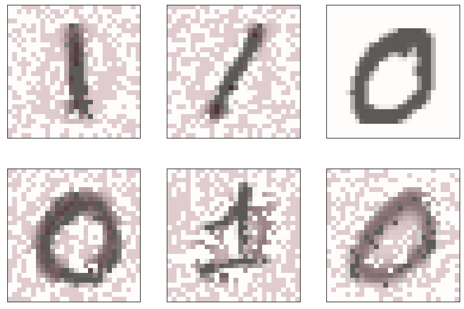
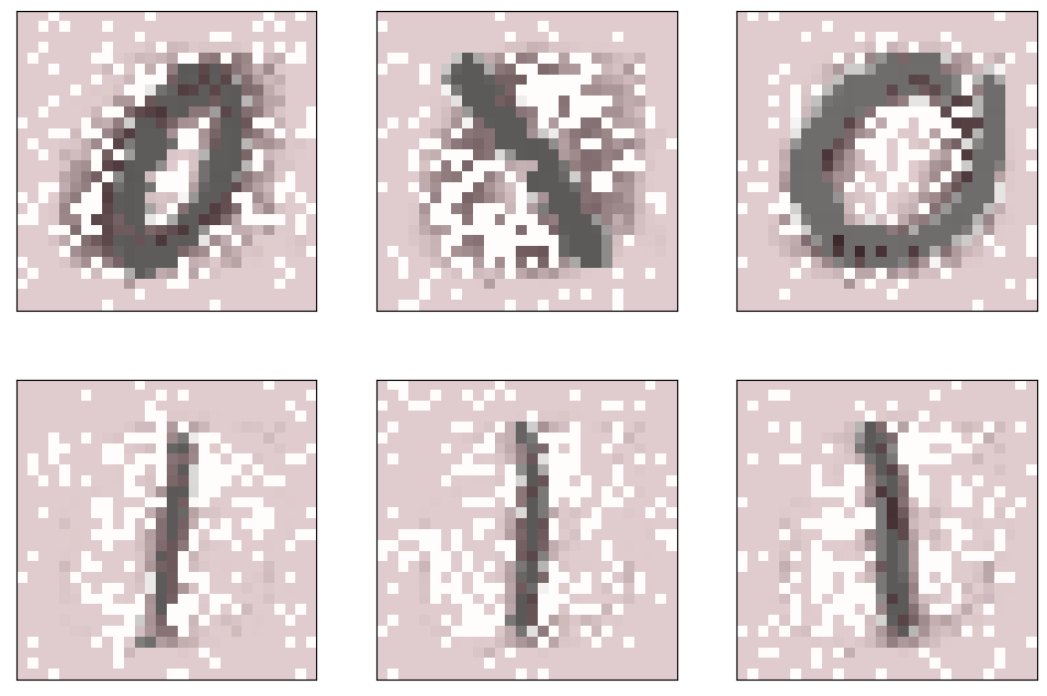
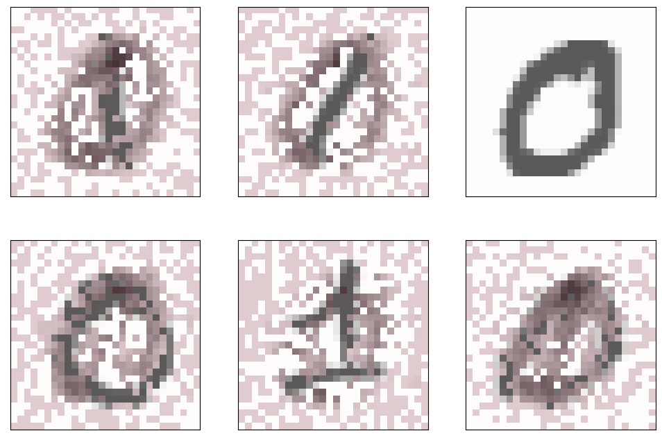
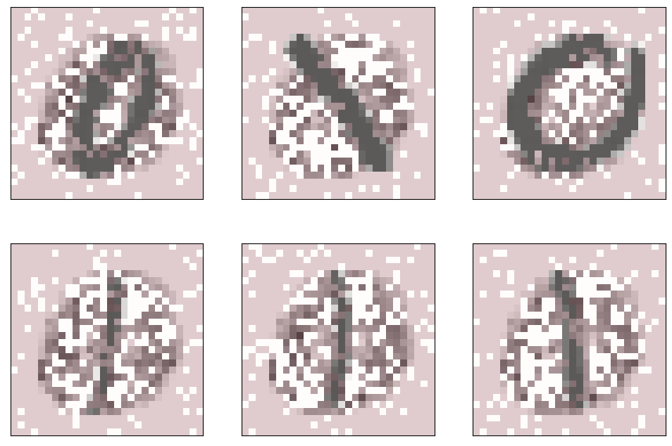
Figure 12: Imputed grayscale images by F3I (first two rows) or mean imputation (last two rows) for the first $6$ samples (trained on the first 600 samples of MNIST with the hyperparameters in Table 8). Positions of red pixels represent missing pixels during the training phase which are imputed by either F3I or mean imputation. Columns 1 to 3 correspond to MCAR-missing pixels (Assumption 3.2), columns 4 to 6 to MAR-missing pixels (Assumption 3.3), and columns 7 to 9 to MNAR-missing pixels (Assumption 3.4). Note that in one of the samples with MAR-missing pixels, no pixel is missing, which is due to randomness in the generation of missing pixels.

Table 10: Overview of the drug repurposing data set PREDICT for joint imputation-classification experiments, with the number of drugs, drug features, percentage of missing drug data, diseases, disease features, percentage of missing disease features, along with the number of positive and negative drug-disease pairs.

Data set	$N_{\text{drugs}}$	$F_{\text{drugs}}$ ($\%$ missing)	$N_{\text{diseases}}$	$F_{\text{users}}$ ($\%$ missing)	Pos	Neg
PREDICT (Réda, 2023a)	1,150	1,642   (24)	1,028	1,490   (26)	4,627	132
PREDIC (reduced)	175	326   (36)	175	215   (60)	454	0

F.2.3 Classification quality (drug repurposing task)

Joint imputation and repurposing.

This time, we consider the drug (item) and disease (user) feature matrices, along with the drug-disease association class labels from another drug repurposing data set, which natively includes missing values in the drug and disease feature matrices. This data set, named PREDICT (Réda, 2023a), is further described in Table 10. All unknown drug-disease associations are labeled $0.5$, whereas positive (respectively, negative) ones are labeled $+1$ (resp., $-1$). To restrict the computational cost, we restricted the data set to its first $500$ ratings (i.e., drug-disease pairs) and to the $350$ features with highest variance across all drugs and diseases. We also add other missing values to the data set via a MCAR mechanism –as we might have lost some missing values when reducing the data set– and run a hyperparameter optimization procedure, similarly to what has been done on the MNIST data set (see Subsection F.2.2). See Table 11 for the selected hyperparameter values.

The corresponding numerical results compared to the mean imputation and NeuMiss (with the same architecture of MLPs) is displayed in Table 12. This table shows that PCGradF3I performs slightly better than NeuMiss on this very difficult data set, while being significantly better than the naive approach relying on the imputation by the mean value. Those results confirm what we observed on the MNIST data set (see Table 9).

Table 11: Fine-tuned hyperparameter values using Optuna to train the MLP block for each imputation method (NeuMiss, Mean imputation, PCGradF3I) on the PREDICT data set. K, T, $\beta$ and $\eta$ are F3I-specific parameters, whereas all remaining parameters are common to all three methods and belong to the MLP block.

Hyperparameter	Number of epochs	Learning rate	MLP depth	K	T	$\beta$	$\eta$
Value	10	0.01	1 layer	12	25	0.246	0.008

Table 12: Area Under the Curve (AUC) values (average $\pm$ standard deviation) in the testing subset in PREDICT (hidden during the training phase) and corresponding tuned hyperparameter values (rounded up to the $3^{\text{rd}}$ decimal place for values in $\mathbb{R}$) for $N=100$ iterations. NeuMiss has been trained on the same number of epochs and the same MLP architecture as PCGradF3I and the mean imputation followed by the MLP (Mean imputation).

Type	$p^{\text{miss}}$	Algorithm	AUC
MCAR (Assumption 3.2)	$50\%$	Mean imputation	0.480 $\pm$0.004
		NeuMiss (Le Morvan et al., 2020)	0.502 $\pm$0.012
		PCGradF3I (ours)	0.505 $\pm$0.009

Figure 23: Imputation of missing values in the drug (left) and disease (right) feature matrices for F3I and its baselines in the DNdataset drug repurposing data set (Gao et al., 2022). The first row shows boxplots of mean-squared errors (MSE) across each algorithm’s $100$ iterations (with different random seeds). In contrast, the second row displays the runtimes (in seconds) across iterations for the imputation step. The average value of MSE and runtime is displayed above each corresponding boxplot. Abbreviations: OT: Optimal Transport-based imputer (Muzellec et al., 2020), KNN: KNN imputer with distance-associated weights (Troyanskaya et al., 2001), Mean: imputation by the feature-wise mean value.

References

- Akiba et al. (2019) Akiba, T., Sano, S., Yanase, T., Ohta, T., and Koyama, M. Optuna: A next-generation hyperparameter optimization framework. In The 25th ACM SIGKDD International Conference on Knowledge Discovery & Data Mining, pp. 2623–2631, 2019.
- Arthur & Vassilvitskii (2006) Arthur, D. and Vassilvitskii, S. k-means++: The advantages of careful seeding. Technical report, Stanford, 2006.
- Auer et al. (2002) Auer, P., Cesa-Bianchi, N., Freund, Y., and Schapire, R. E. The nonstochastic multiarmed bandit problem. SIAM Journal on Computing, 32(1):48–77, 2002. doi: 10.1137/S0097539701398375. URL https://doi.org/10.1137/S0097539701398375.
- Ayme et al. (2023) Ayme, A., Boyer, C., Dieuleveut, A., and Scornet, E. Naive imputation implicitly regularizes high-dimensional linear models. In International Conference on Machine Learning, pp. 1320–1340. PMLR, 2023.
- Ayme et al. (2024) Ayme, A., Boyer, C., Dieuleveut, A., and Scornet, E. Random features models: a way to study the success of naive imputation. arXiv preprint arXiv:2402.03839, 2024.
- Bentley (1975) Bentley, J. L. Multidimensional binary search trees used for associative searching. Commun. ACM, 18(9):509–517, sep 1975. ISSN 0001-0782. doi: 10.1145/361002.361007. URL https://doi.org/10.1145/361002.361007.
- Beretta & Santaniello (2016) Beretta, L. and Santaniello, A. Nearest neighbor imputation algorithms: a critical evaluation. BMC medical informatics and decision making, 16:197–208, 2016.
- Bergstra et al. (2011) Bergstra, J., Bardenet, R., Bengio, Y., and Kégl, B. Algorithms for hyper-parameter optimization. In Shawe-Taylor, J., Zemel, R., Bartlett, P., Pereira, F., and Weinberger, K. (eds.), Advances in Neural Information Processing Systems, volume 24. Curran Associates, Inc., 2011. URL https://proceedings.neurips.cc/paper_files/paper/2011/file/86e8f7ab32cfd12577bc2619bc635690-Paper.pdf.
- Cardano et al. (1968) Cardano, G., Witmer, T. R., and Ore, Ø. Ars magna, or, The rules of algebra. Dover, New York, 1968. ISBN 9780486678115; 0486678113.
- Cesa-Bianchi & Lugosi (2006) Cesa-Bianchi, N. and Lugosi, G. Prediction, learning, and games. Cambridge university press, 2006.
- Chen et al. (2018) Chen, Z., Badrinarayanan, V., Lee, C.-Y., and Rabinovich, A. GradNorm: Gradient normalization for adaptive loss balancing in deep multitask networks. In Dy, J. and Krause, A. (eds.), Proceedings of the 35th International Conference on Machine Learning, volume 80 of Proceedings of Machine Learning Research, pp. 794–803. PMLR, 10–15 Jul 2018. URL https://proceedings.mlr.press/v80/chen18a.html.
- De Rooij et al. (2014) De Rooij, S., Van Erven, T., Grünwald, P. D., and Koolen, W. M. Follow the leader if you can, hedge if you must. The Journal of Machine Learning Research, 15(1):1281–1316, 2014.
- Degenne et al. (2020) Degenne, R., Ménard, P., Shang, X., and Valko, M. Gamification of pure exploration for linear bandits. In International Conference on Machine Learning, pp. 2432–2442. PMLR, 2020.
- Emmanuel et al. (2021) Emmanuel, T., Maupong, T., Mpoeleng, D., Semong, T., Mphago, B., and Tabona, O. A survey on missing data in machine learning. Journal of Big data, 8:1–37, 2021.
- Gao et al. (2022) Gao, C.-Q., Zhou, Y.-K., Xin, X.-H., Min, H., and Du, P.-F. Dda-skf: predicting drug–disease associations using similarity kernel fusion. Frontiers in Pharmacology, 12:784171, 2022.
- Ipsen et al. (2021) Ipsen, N. B., Mattei, P.-A., and Frellsen, J. not-{miwae}: Deep generative modelling with missing not at random data. In International Conference on Learning Representations, 2021. URL https://openreview.net/forum?id=tu29GQT0JFy.
- Jarrett et al. (2022) Jarrett, D., Cebere, B. C., Liu, T., Curth, A., and van der Schaar, M. Hyperimpute: Generalized iterative imputation with automatic model selection. In International Conference on Machine Learning, pp. 9916–9937. PMLR, 2022.
- Joel et al. (2024) Joel, L. O., Doorsamy, W., and Paul, B. S. On the performance of imputation techniques for missing values on healthcare datasets. arXiv preprint arXiv:2403.14687, 2024.
- Koren et al. (2021) Koren, Y., Rendle, S., and Bell, R. Advances in collaborative filtering. Recommender systems handbook, pp. 91–142, 2021.
- Kyono et al. (2021) Kyono, T., Zhang, Y., Bellot, A., and van der Schaar, M. Miracle: Causally-aware imputation via learning missing data mechanisms. Advances in Neural Information Processing Systems, 34:23806–23817, 2021.
- Lattimore & Szepesvári (2020) Lattimore, T. and Szepesvári, C. Bandit algorithms. Cambridge University Press, 2020.
- Le Morvan & Varoquaux (2024) Le Morvan, M. and Varoquaux, G. Imputation for prediction: beware of diminishing returns. arXiv preprint arXiv:2407.19804, 2024.
- Le Morvan et al. (2020) Le Morvan, M., Josse, J., Moreau, T., Scornet, E., and Varoquaux, G. Neumiss networks: differentiable programming for supervised learning with missing values. Advances in Neural Information Processing Systems, 33:5980–5990, 2020.
- Le Morvan et al. (2021) Le Morvan, M., Josse, J., Scornet, E., and Varoquaux, G. What’sa good imputation to predict with missing values? Advances in Neural Information Processing Systems, 34:11530–11540, 2021.
- LeCun et al. (1998) LeCun, Y., Cortes, C., and Burges, C. The mnist database of handwritten digits. https://drive.google.com/file/d/1eEKzfmEu6WKdRlohBQiqi3PhW_uIVJVP/view, 1998.
- Liu et al. (2021) Liu, B., Liu, X., Jin, X., Stone, P., and Liu, Q. Conflict-averse gradient descent for multi-task learning. Advances in Neural Information Processing Systems, 34:18878–18890, 2021.
- Luo et al. (2016) Luo, H., Wang, J., Li, M., Luo, J., Peng, X., Wu, F.-X., and Pan, Y. Drug repositioning based on comprehensive similarity measures and bi-random walk algorithm. Bioinformatics, 32(17):2664–2671, 2016.
- Luo et al. (2018) Luo, Y., Cai, X., Zhang, Y., Xu, J., et al. Multivariate time series imputation with generative adversarial networks. Advances in neural information processing systems, 31, 2018.
- Mattei & Frellsen (2019) Mattei, P.-A. and Frellsen, J. MIWAE: Deep generative modelling and imputation of incomplete data sets. In Chaudhuri, K. and Salakhutdinov, R. (eds.), Proceedings of the 36th International Conference on Machine Learning, volume 97 of Proceedings of Machine Learning Research, pp. 4413–4423. PMLR, 09–15 Jun 2019. URL https://proceedings.mlr.press/v97/mattei19a.html.
- Mazumder et al. (2010) Mazumder, R., Hastie, T., and Tibshirani, R. Spectral regularization algorithms for learning large incomplete matrices. The Journal of Machine Learning Research, 11:2287–2322, 2010.
- Mohan et al. (2018) Mohan, K., Thoemmes, F., and Pearl, J. Estimation with incomplete data: The linear case. In Proceedings of the International Joint Conferences on Artificial Intelligence Organization, 2018.
- Muzellec et al. (2020) Muzellec, B., Josse, J., Boyer, C., and Cuturi, M. Missing data imputation using optimal transport. In International Conference on Machine Learning, pp. 7130–7140. PMLR, 2020.
- Pedregosa et al. (2011) Pedregosa, F., Varoquaux, G., Gramfort, A., Michel, V., Thirion, B., Grisel, O., Blondel, M., Prettenhofer, P., Weiss, R., Dubourg, V., Vanderplas, J., Passos, A., Cournapeau, D., Brucher, M., Perrot, M., and Duchesnay, E. Scikit-learn: Machine learning in Python. Journal of Machine Learning Research, 12:2825–2830, 2011.
- Rubin (1976) Rubin, D. B. Inference and missing data. Biometrika, 63(3):581–592, 1976.
- Réda (2023a) Réda, C. Predict drug repurposing dataset. doi: 10.5281/zenodo.7983090, 2023a. URL https://doi.org/10.5281/zenodo.7983090.
- Réda (2023b) Réda, C. Transcript drug repurposing dataset. doi: 10.5281/zenodo.7982976, 2023b. URL https://doi.org/10.5281/zenodo.7982976.
- Seu et al. (2022) Seu, K., Kang, M.-S., and Lee, H. An intelligent missing data imputation techniques: A review. JOIV: International Journal on Informatics Visualization, 6(1-2):278–283, 2022.
- Śmieja et al. (2018) Śmieja, M., Struski, Ł., Tabor, J., Zieliński, B., and Spurek, P. Processing of missing data by neural networks. Advances in neural information processing systems, 31, 2018.
- Sportisse et al. (2020) Sportisse, A., Boyer, C., and Josse, J. Estimation and imputation in probabilistic principal component analysis with missing not at random data. Advances in Neural Information Processing Systems, 33:7067–7077, 2020.
- Stekhoven & Bühlmann (2012) Stekhoven, D. J. and Bühlmann, P. Missforest—non-parametric missing value imputation for mixed-type data. Bioinformatics, 28(1):112–118, 2012.
- Tang et al. (2003) Tang, G., Little, R. J., and Raghunathan, T. E. Analysis of multivariate missing data with nonignorable nonresponse. Biometrika, 90(4):747–764, 2003.
- Tashiro et al. (2021) Tashiro, Y., Song, J., Song, Y., and Ermon, S. Csdi: Conditional score-based diffusion models for probabilistic time series imputation. Advances in Neural Information Processing Systems, 34:24804–24816, 2021.
- Tiao et al. (2021) Tiao, L. C., Klein, A., Seeger, M. W., Bonilla, E. V., Archambeau, C., and Ramos, F. Bore: Bayesian optimization by density-ratio estimation. In International Conference on Machine Learning, pp. 10289–10300. PMLR, 2021.
- Troyanskaya et al. (2001) Troyanskaya, O., Cantor, M., Sherlock, G., Brown, P., Hastie, T., Tibshirani, R., Botstein, D., and Altman, R. B. Missing value estimation methods for dna microarrays. Bioinformatics, 17(6):520–525, 2001.
- van Buuren & Groothuis-Oudshoorn (2011) van Buuren, S. and Groothuis-Oudshoorn, K. mice: Multivariate imputation by chained equations in r. Journal of Statistical Software, 45(3):1–67, 2011. doi: 10.18637/jss.v045.i03.
- van Loon et al. (2024) van Loon, W., Fokkema, M., de Vos, F., Koini, M., Schmidt, R., and de Rooij, M. Imputation of missing values in multi-view data. Information Fusion, pp. 102524, 2024.
- Vershynin (2018) Vershynin, R. High-dimensional probability: An introduction with applications in data science, volume 47. Cambridge university press, 2018.
- Virtanen et al. (2020) Virtanen, P., Gommers, R., Oliphant, T. E., Haberland, M., Reddy, T., Cournapeau, D., Burovski, E., Peterson, P., Weckesser, W., Bright, J., van der Walt, S. J., Brett, M., Wilson, J., Millman, K. J., Mayorov, N., Nelson, A. R. J., Jones, E., Kern, R., Larson, E., Carey, C. J., Polat, İ., Feng, Y., Moore, E. W., VanderPlas, J., Laxalde, D., Perktold, J., Cimrman, R., Henriksen, I., Quintero, E. A., Harris, C. R., Archibald, A. M., Ribeiro, A. H., Pedregosa, F., van Mulbregt, P., and SciPy 1.0 Contributors. SciPy 1.0: Fundamental Algorithms for Scientific Computing in Python. Nature Methods, 17:261–272, 2020. doi: 10.1038/s41592-019-0686-2.
- Vo et al. (2024) Vo, V., Zhao, H., Le, T., Bonilla, E. V., and Phung, D. Optimal transport for structure learning under missing data. arXiv preprint arXiv:2402.15255, 2024.
- Yoon et al. (2018) Yoon, J., Jordon, J., and Schaar, M. Gain: Missing data imputation using generative adversarial nets. In International conference on machine learning, pp. 5689–5698. PMLR, 2018.
- Yu et al. (2020) Yu, T., Kumar, S., Gupta, A., Levine, S., Hausman, K., and Finn, C. Gradient surgery for multi-task learning. In Larochelle, H., Ranzato, M., Hadsell, R., Balcan, M., and Lin, H. (eds.), Advances in Neural Information Processing Systems, volume 33, pp. 5824–5836. Curran Associates, Inc., 2020. URL https://proceedings.neurips.cc/paper_files/paper/2020/file/3fe78a8acf5fda99de95303940a2420c-Paper.pdf.