Matrix Completion in Group Testing:
Bounds and Simulations

Abstract

The main goal of group testing is to identify a small number of defective items in a large population of items. A test on a subset of items is positive if the subset contains at least one defective item and negative otherwise. In non-adaptive design, all tests can be tested simultaneously and represented by a measurement matrix in which a row and a column represent a test and an item, respectively. An entry in row $i$ and column $j$ is 1 if item $j$ belongs to the test $i$ and is 0 otherwise. Given an unknown set of defective items, the objective is to design a measurement matrix such that, by observing its corresponding outcome vector, the defective items can be recovered efficiently. The basic trait of this approach is that the measurement matrix has remained unchanged throughout the course of generating the outcome vector and recovering defective items. In this paper, we study the case in which some entries in the measurement matrix are erased, called the missing measurement matrix, before the recovery phase of the defective items, and our objective is to fully recover the measurement matrix from the missing measurement matrix. In particular, we show that some specific rows with erased entries provide information aiding the recovery while others do not. Given measurement matrices and erased entries follow the Bernoulli distribution, we show that before the erasing event happens, sampling sufficient sets of defective items and their corresponding outcome vectors can help us recover the measurement matrix from the missing measurement matrix.

I Introduction

Group testing is a combinatorial optimization problem whose objective is to identify a small number of defective items in a large population of items efficiently [1]. Defective items and non-defective (negative) items are defined by context. For example, in the Covid-19 scenario, defective (respectively, non-defective) items are people who are positive (respectively, negative) for Coronavirus. In standard group testing (GT), the outcome of the test on a subset of items is positive if the subset contains at least one defective item and negative otherwise. In this paper, we study the case in which some entries in the measurement matrix are erased and sets of input items and their corresponding test outcomes are observed (sampled). Our objective is to fully recover the measurement matrix by using this information.

I-A Motivation

Building fully structural neuronal connectivity to better understand the structural-functional relationship of the brain is the main objective of connectome [2]. For each person, building their fully structural neuronal connectivity when they are healthy can potentially help doctors treat them more easily when their brain does not function properly. Even in the case the doctors do not have their neuronal connectivity when they were healthy, having their neuronal connectivity when they are admitted to the hospital also helps them to identify causes by comparing it with other existing neuronal connectivities.

The most commonly used technique among them is functional Magnetic Resonance Imaging (fMRI), which offers an in-vivo view of both the brain’s structure and function. Typically, there are three levels of resolutions: marco, meso, and micro. The macro level encompasses broad brain regions and the long-distance connections between them. The micro level focuses on cellular and neuronal details. To bridge the gap between the fine-grained details of individual neurons (micro level) and the more global connections between brain regions (macro level), the meso level is considered. At this level, one provides the network of connections between groups of neurons and local brain structures, such as cortical minicolumns and neural subnetworks. To construct a micro connectome, it is compulsory to know whether there exists a synapse between two neurons (the site where the axon of a neuron innervates to another neuron is called a synaptic site). A neuron that sends (respectively, receives) signals to another neuron across a synapse is called the presynaptic (respectively, postsynaptic) neuron. It is common to build connectome at meso or macro levels rather than a micro level because the brain is populated with roughly $100$ billion neurons [3] and this makes building a micro connectome nearly infeasible. However, with the recent development of neural population recordings, it is possible to record tens of thousands of neurons from (mouse) cortex during spontaneous, stimulus-evoked, and task-evoked epochs [4, 5]. This could enable the recording of most of the neurons in a brain region in the near future and thus could provide a sufficiently large number of observations with a set of presynaptic neurons spiked by an input stimulus and a set of postsynaptic neurons responded to the spiked presynaptic neurons, i.e., the input stimulus.

To construct a complete connectome of a brain, we present the neuron-neuron connectivities based on [6] as follows. Let $\mathbf{T}=(t_{ij})$ be an $(n+t)\times(n+t)$ connectivity matrix of $n+t$ neurons. Entry $t_{ij}=1$ means there is a synaptic connection starting from neuron $i$ to neuron $j$, i.e., neuron $i$ is a presynaptic neuron and neuron $j$ is a postsynaptic neuron. On the other hand, $t_{ij}=1$ means there is no synaptic connection starting from neuron $i$ to neuron $j$. Note that $\mathbf{T}$ may not be symmetric. Since a stimulus can be stored as a memory at a few synapses [7, 8, 9], a synapse can be determined by knowing which neurons participate in responding to the stimulus. Therefore, we can identify the synaptic connection between two neurons by dividing the neuron set into a set of a small number of presynaptic neurons and a set of a large number of postsynaptic neurons to observe their responses to a stimulus. In particular, we can create a $t\times n$ binary presynaptic-postsynaptic connectivity matrix $\mathbf{M}=(m_{ij})$ as follows. Let $\mathcal{S}\subseteq[n+t]=\{1,2,\ldots,n+t\}$ with $|\mathcal{S}|=t$ be a set of presynaptic neurons and $\overline{\mathcal{S}}=[n+t]\setminus\mathcal{S}$ with $|\overline{\mathcal{S}}|=n$ be the set of postsynaptic neurons corresponding to the set of presynaptic neurons $\mathcal{S}$. Matrix $\mathbf{M}$ is obtained by removing every column $j\in S$ and every row $i\in\overline{\mathcal{S}}$ in $\mathbf{M}$. It directly follows that entry $m_{ij}=1$ means there is a connection between the presynaptic neuron $i$ and the postsynaptic neuron $j$, and $m_{ij}=0$ means otherwise.

Given a set of $n$ postsynaptic neurons labeled from $1$ to $n$, let $\mathcal{X}\subseteq\{0,1\}^{n}$ be the discretized stimulus space (the ambient space) representing all stimuli. For any vector $\mathbf{v}=(v_{1},\ldots,v_{n})\in\{0,1\}^{n}$, $v_{j}=1$ means the postsynaptic neuron $j$ spikes and $v_{j}=0$ means otherwise. Let $\mathbf{x}=(x_{1},\ldots,x_{n})\in\mathcal{X}$ be the binary representation vector for an input stimulus. Given a fixed set of $t$ presynaptic neurons labeled $\{1,\ldots,t\}=[t]$, let $\mathbf{y}=(y_{1},\ldots,y_{t})\in\mathcal{Y}\subseteq\{0,1\}^{t}$ be the encoded vector for the input stimulus. For simplicity, we use a model proposed by Bui [6] as follows: every presynaptic neuron spikes, and a postsynaptic neuron spikes if it does not connect to an inhibitory presynaptic neuron. Specifically, $y_{i}=0$ means the presynaptic neuron $i$ is inhibitory and spiking, and $y_{i}=1$ means the presynaptic neuron $i$ is excitatory and spiking. Note that every presynaptic neuron $i$ is a hybrid neuron, i.e., depending on the value of $y_{i}$, it can behave either as an excitatory neuron or an inhibitory neuron. A stimulus represented by $\mathbf{x}$ is encoded at the $t$ presynaptic neurons as $\mathbf{y}$. This model can be illustrated in Fig. 1.

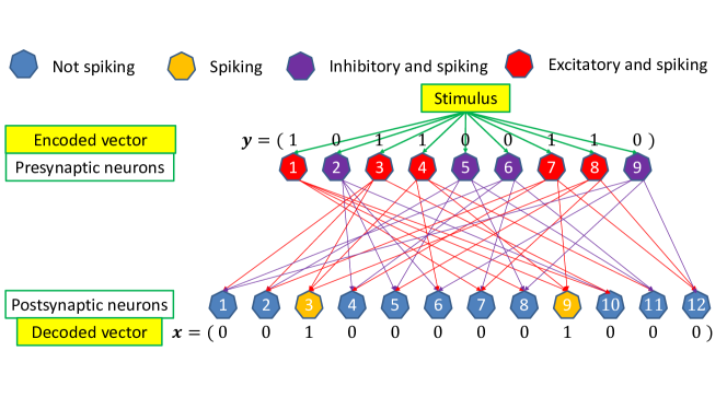
Figure 1: There are 21 neurons in total. They are divided into a set of 9 presynaptic neurons and a set of 12 postsynaptic neurons. The input stimulus is encoded by the presynaptic neurons and denoted as $\mathbf{y}=(1,0,1,1,0,0,1,1,0)$ in which $y_{i}=1$ means the $i$th presynaptic neuron is excitatory and spiking while $y_{i}=0$ means the $i$th presynaptic neuron is inhibitory and spiking. The encoded stimulus is then decoded by the postsynaptic neurons and denoted as $\mathbf{x}=(0,0,1,0,0,0,0,0,1,0,0,0)$ in which $x_{j}=1$ means the $j$th postsynaptic neuron spikes while $x_{j}=0$ means the $j$th postsynaptic neuron does not spike.

The corresponding $t\times n$ binary presynaptic-postsynaptic connectivity matrix $\mathbf{M}=(m_{ij})$ is:

$$\mathbf{M}=\left[\begin{array}[]{cccccccccccc}0&0&0&0&0&1&1&1&1&0&0&0\\ 0&0&0&1&1&1&0&0&0&1&0&0\\ 1&1&1&0&0&0&0&0&0&1&0&0\\ 0&0&1&0&0&1&0&0&1&0&1&0\\ 0&1&0&0&1&0&0&1&0&0&1&0\\ 1&0&0&1&0&0&1&0&0&0&1&0\\ 0&1&0&0&0&0&1&0&1&0&0&1\\ 0&1&0&0&1&0&1&0&0&0&0&1\\ 1&0&0&0&0&1&0&1&0&0&0&1\end{array}\right],\mathbf{M}^{\blacksquare}=\left[\begin{array}[]{cccccccccccc}0&0&0&0&0&1&1&1&1&0&0&0\\ 0&0&\blacksquare&\blacksquare&1&1&0&0&0&1&0&0\\ 1&1&1&0&0&0&0&0&0&1&0&0\\ 0&0&1&0&0&1&0&0&1&0&1&0\\ 0&1&\blacksquare&0&1&\blacksquare&0&1&0&0&1&0\\ 1&0&0&\blacksquare&0&0&1&0&0&0&1&0\\ 0&1&0&0&0&0&1&0&1&0&0&1\\ 0&1&0&0&1&0&1&0&0&0&0&1\\ 1&0&0&0&0&1&0&1&0&0&0&1\end{array}\right]$$ (1)

To distinguish two distinct stimuli, it is natural that any two distinct stimuli are represented by two distinct vectors in $\mathcal{X}$ and are encoded by two distinct vectors in $\mathcal{Y}$. Then there exists a bijective mapping from $\mathbf{M}$ and $\mathbf{x}$ to $\mathbf{y}$ and let us denote it $\mathbf{y}:=\mathbf{M}\odot\mathbf{x}$, where $\odot$ is the mapping function. For $\mathbf{v}=(v_{1},v_{2},\ldots,v_{p})$, Let $\mathsf{supp}(\mathbf{v}):=\{j\in[p]\mid v_{j}=1\}$ be the characteristic set of vector $\mathbf{v}$. Then for any $j\in\mathsf{supp}(\mathbf{x})$, we must have $\mathsf{supp}(\mathbf{M}(:,j))\subseteq\mathsf{supp}(\mathbf{y})$. Indeed, if there exists row $i_{0}$ such that $m_{i_{0}j}=1$ and $y_{i_{0}}=0$, $x_{j}$ must equal to 0 because of the decoding rule. This contradicts the fact that $j\in\mathsf{supp}(\mathbf{x})$. Therefore, we get

$$\mathbf{y}=\bigvee_{j\in\mathsf{supp}(\mathbf{x})}\mathbf{M}(:,j),$$ (2)

and the mapping function $\odot$ is thus the testing operation in group testing.

Although the fast-paced development of neural recording could promise a complete connectome reconstruction, it is still impossible to identify some synaptic connections because of the obscured nature of these synapses. Let us denote these synapses erased synapses. Let $r$ be the total number of unidentified synapses and $\overline{\Psi}=\{(i_{1},j_{1}),\ldots,(i_{r},j_{r})\}$ be their corresponding set, where $1\leq i_{k}\leq t$ and $1\leq j_{k}\leq n$ for any $(i_{k},j_{k})\in\overline{\Psi}$. Let $\blacksquare$ be an erasure that cannot be determined to be 0 or 1. Then the presynaptic-postsynaptic connectivity matrix obtained by experiments is thus $\mathbf{M}^{\blacksquare}=(m^{\blacksquare}_{ij})$ as illustrated in (1), where $m^{\blacksquare}_{ij}=m_{ij}$ if $(i,j)\not\in\overline{\Psi}$ and $m^{\blacksquare}_{ij}=\blacksquare$ if $(i,j)\in\overline{\Psi}$. Note that for any stimulus $\mathbf{y}$, one always receives $\mathbf{x}:=\mathrm{dec}(\mathbf{M}^{\blacksquare},\mathbf{y})$ though we do not know every entry in $\mathbf{M}^{\blacksquare}$. More importantly, because of spontaneous neural activity, we cannot control stimulus inputs as we wish because we do not know which spiking neurons represent a stimulus in general. In other words, it is infeasible to generate a stimulus that induces the corresponding $\mathbf{x}$ or $\mathbf{y}$ as wanted. The problem of reconstructing the complete connectome turns out to be the problem of reconstructing $\mathbf{M}$ from $\mathbf{M}^{\blacksquare}$ by collecting enough pairs $(\mathbf{x},\mathbf{y})$ in group testing.

I-B Problem formulation

We index the population of $n$ items from $1$ to $n$. Let $[n]:=\{1,2,\ldots,n\}$ and $\mathcal{D}$ be the defective set with $|\mathcal{D}|=d$. A test on a subset of items $\mathcal{S}\subseteq[n]$ is positive if the subset contains at least one defective item and negative otherwise. In other words, the test outcome, denoted as $\mathsf{test}(\mathcal{S})$, is positive if $|\mathcal{S}\cap\mathcal{D}|\geq 1$ and negative if $|\mathcal{S}\cap\mathcal{D}|=0$. Note that $|\mathcal{D}|\geq 1$ because if $|\mathcal{D}|=0$ then all tests yield negative.

In the non-adaptive setting, tests are usually represented by a $t\times n$ binary measurement matrix $\mathbf{M}=(m_{ij})\in\{0,1\}^{t\times n}$, where $n$ is the number of items and $t$ is the number of tests. An input vector $\mathbf{x}=(x_{1},\ldots,x_{n})^{T}\in\{0,1\}^{n}$ represents $n$ items in which $x_{j}=1$ if item $j$ is defective and $x_{j}=0$ otherwise for $j\in[n]$. The $j$th item corresponds to the $j$th column of the matrix. An entry $m_{ij}=1$ means that item $j$ belongs to test $i$, and $m_{ij}=0$ means otherwise. The outcome of all tests is $\mathbf{y}=(y_{1},\ldots,y_{t})^{T}$, where $y_{i}=1$ if test $i$ is positive and $y_{i}=0$ otherwise. The procedure to produce the measurement matrix $\mathbf{M}$ is called construction, the procedure to obtain the outcomes of all tests using the measurement matrix is called encoding, and the procedure to recover positive items from the outcomes is called decoding.

Let $\mathsf{supp}(\mathbf{v})=\{j\mid v_{j}\neq 0\}$ be the support set for vector $\mathbf{v}=(v_{1},\ldots,v_{w})$ and $\mathcal{M}_{i}=\mathsf{supp}(\mathbf{M}(i,:))$ for $i=1,\ldots,t$. The OR-wise operator between two vectors of same size $\mathbf{z}=(z_{1},\ldots,z_{n})$ and $\mathbf{z}^{\prime}=(z_{1}^{\prime},\ldots,z_{n}^{\prime})$ is $\mathbf{z}\vee\mathbf{z}^{\prime}=(z_{1}\vee z_{1}^{\prime},\ldots,z_{n}\vee z_{n}^{\prime})$. Then the outcome vector $\mathbf{y}$ is given by

$$\mathbf{y}:=\begin{bmatrix}y_{1}\\ \vdots\\ y_{t}\end{bmatrix} := \mathbf{M}\odot\mathbf{x} :=\begin{bmatrix}\mathbf{M}(1,:)\otimes\mathbf{x}\\ \vdots\\ \mathbf{M}(t,:)\otimes\mathbf{x}\end{bmatrix}$$

$$:= \mathsf{test}(\mathbf{M},\mathsf{supp}(\mathbf{x})) :=\begin{bmatrix}\mathsf{test}(\mathcal{M}_{1}\cap\mathsf{supp}(\mathbf{x}))\\ \vdots\\ \mathsf{test}(\mathcal{M}_{t}\cap\mathsf{supp}(\mathbf{x}))\end{bmatrix},$$

where $\odot$ and $\mathsf{test}(\cdot)$ are notations for the test operations in group testing; namely, $y_{i}:=\mathbf{M}(i,:)\odot\mathbf{x}:=\mathsf{test}(\mathcal{M}_{i}\cap\mathsf{supp}(\mathbf{x}))=1$ if $|\mathcal{M}_{i}\cap\mathsf{supp}(\mathbf{x})|\geq 1$ and $y_{i}=0$ if $|\mathcal{M}_{i}\cap\mathsf{supp}(\mathbf{x})|=0$, for $i=1,\ldots,t$. The procedure to get outcome vector $\mathbf{y}$ is called encoding and the procedure to recover $\mathbf{x}$ from $\mathbf{y}$ and $\mathbf{M}$ is called decoding.

Let $\blacksquare$ be an erasure that cannot be determined to be 0 or 1. Let $\Psi=\{\Psi_{1},\Psi_{2},\dots,\Psi_{r}\}\subseteq[tn]$ be the set of missing (erased) entries from left to right and from top to bottom in $\mathbf{M}$. In particular, for any $\Psi_{g}\in\Psi$, if $\Psi_{g}=(i_{g}-1)n+j_{g}$ where $i_{g}\in\{1,\dots,t\}$ and $j_{g}\in\{1,\dots,n\}$ then $\Psi_{g}$ is located at row $i_{g}$ and column $j_{g}$. Let $\overline{\Psi}=\{(i_{1},j_{1}),\ldots,(i_{r},j_{r})\}$ be the bijective mapping set of $\Psi$, where $a_{g}=(i_{g}-1)n+j_{g}$ is represented by the pair $(i_{g},j_{g})$ and vice versa for $g\in[r]$. Let $\mathbf{\psi}=(\psi_{1},\ldots,\psi_{r})^{T}\in\{0,1\}^{r}$ be the characteristic vector of $\overline{\Psi}$ in which $\psi_{g}=m_{i_{g}j_{g}}$ for $(i_{g},j_{g})\in\overline{\Psi}$. The missing matrix $\mathbf{M}^{\blacksquare}=(m^{\blacksquare}_{ij})$ induced from $\mathbf{M}$ is defined as follows: $m^{\blacksquare}_{ij}=m_{ij}$ if $(i,j)\not\in\overline{\Psi}$ and $m^{\blacksquare}_{ij}=\blacksquare$ if $(i,j)\in\overline{\Psi}$.

Let $\mathcal{T}_{d}:=\{\mathbf{x}\in\{0,1\}^{n}\mid|\mathbf{x}|=d\}$ be the set of all binary vectors of length $n$ and weight $d$ and $\chi:=\{\mathbf{x}_{1},\mathbf{x}_{2},\ldots,\mathbf{x}_{s}\}\subseteq\mathcal{T}_{d}$ be a set of input vectors that are sampled uniformly and identically from $\mathcal{T}_{d}$. Let $\gamma:=\{\mathbf{y}_{1}:=\mathbf{M}\odot\mathbf{x}_{1},\mathbf{y}_{2}:=\mathbf{M}\odot\mathbf{x}_{2},\ldots,\mathbf{y}_{s}:=\mathbf{M}\odot\mathbf{x}_{s}\}$ be the set of the outcome vectors corresponding to the input vectors in $\chi$. Our objective is to estimate the possibility of recovering $\mathbf{M}$ given the missing matrix $\mathbf{M}^{\blacksquare}$ and the number of input and outcome vectors $(\mathbf{x},\mathbf{y})\in\chi\times\gamma$ observed. In other words, our objective is to recover $\mathbf{\psi}$.

In order to facilitate understanding of the problem, we assume matrix $\mathbf{M}=(m_{ij})$ and missing entries are generated from the Bernoulli distribution. In particular, for any $i\in[t]$ and $j\in[n]$, $\Pr(m_{ij}=1)=p$, $\Pr(m_{ij}=0)=1-p$, and $\Pr((i,j)\in\overline{\Psi})=q$, where $0<p,q<1$.

I-C Related work

I-C1 Summary of criteria

There are several criteria for tackling group testing, but we focus on four main ones here. The first criterion is the testing design, which can be either non-adaptive or adaptive. In a non-adaptive design, all tests are predetermined and independent, allowing them to be executed in parallel to save time. In contrast, an adaptive design involves tests that depend on the previous tests, often requiring multiple stages. While this design can achieve the information-theoretic bound on the number of tests, it tends to be time-consuming due to the need for multiple stages. The second criterion is the setting of the defective set. In a combinatorial setting, the defective set is arbitrarily organized subject to predefined constraints, whereas in a probabilistic setting, a distribution is applied to the input items. The third important criterion is whether the design is deterministic or randomized. A deterministic design produces the same result given the same inputs, whereas a randomized design introduces a degree of randomness, which may lead to different results when executed multiple times. Finally, the fourth criterion involves the recovery approach: exact recovery, where all defective items are identified, and approximate recovery, where only some of the defective items are identified. Since we consider a variant of group testing, the recovery criterion is not considered in this work. In fact, we consider non-adaptive and probabilistic designs, combinatorial setting.

I-C2 Overview of literature

Group testing: Since the inception of group testing, it has been applied in various fields such as computational and molecular biology [10], networking [11], and Covid-19 testing [12]. For combinatorial group testing with non-adaptive designs, a strong factor of $d^{2}$ has been established in the number of tests [13, 14, 15]. For exact recovery, it is possible to obtain $O(d^{2}\log n)$ tests that can be decoded in time $O(tn)$ with explicit construction [16] or in $\mathsf{poly}(d,\log{n})$ [17, 18, 19, 20] with additional constraints on construction. To reduce the factor $d^{2}$ to $d$, an adaptive design or a probabilistic setting can be used. The set of defective items can be fully recovered by using $O(d\log{(n/d)})$ tests with $O(\log_{d}{n})$ stages in [10] or with two stages in [21]. When the test outcomes are unreliable, it is still possible to obtain $O(d\log{(n/d)})$ tests using a few stages [22, 23, 24, 25, 26]. For probabilistic group testing with non-adaptive design, the number of tests $O(d\log{n})$ has been known for a long time[27, 28, 29, 30]. Decoding time associated with that number of tests has gradually reduced from $\mathsf{poly}(d,\log{n})$ to near-optimal $O(d\log{n})$ [20, 31]. Many variants of group testing such as threshold group testing [32], quantitative group testing [33], complex group testing [34], concomitant group testing [35], and community-aware group testing [36] has also been considered recently. However, to the best of our knowledge, all of these models are not closely related to our setup.

Matrix completion: A closely related research topic to our work is matrix completion which was first known as Netflix problem [37]. In this problem, Netflix database consists of about $t\approx 10^{6}$ users and about $n\approx 25,000$ movies with users rating movies. Suppose that $\mathbf{M}_{t\times n}$ is the (unknown) users rating matrix that we are seeking for. Since most of the users have only seen a small fraction of the movies, only a small subset of entries in $\mathbf{M}$ have been identified and the rest are considered as erased entries. The actual ratings are recorded into matrix $\mathbf{M}^{\blacksquare}=(m_{ij})\in\{\mathbb{R}\cup\{\blacksquare\}\}^{t\times n}$. The goal is to predict which movies a particular user might like. Mathematically, we would like to complete matrix $\mathbf{M}^{\blacksquare}$, i.e., replacing erased entries by users rates, based on the partial observations of some of its entries to reconstruct $\mathbf{M}$. Once $\mathbf{M}$ is low-rank, it is possible to complete the matrix and recover the entries that have not been seen with high probability [38]. In particular, if $\mbox{rank}(\mathbf{M})=k$, $n^{*}=\max(t,n)$, and each entry is observed uniformly, then there are numerical constants $C$ and $c$ such that if the number of observed entries is at least $C(n^{*})^{5/4}k\log{n^{*}}$, all erased entries in $\mathbf{M}^{\blacksquare}$ can be recovered with probability at least $1-cn^{-3}\log{n}$. Following this pioneering work, there is much work to tackle this problem with the same settings or different settings [39, 40, 41, 42]. Unfortunately, the results in [38] are inefficient when $k=O(t)$ because every entry must be observed in that case. Moreover, it is not utilized whether the erased entries are zero or non-zero. Although recovering measurement matrices in group testing is equivalent to the matrix completion problem, the settings in group testing are different from the settings in the standard matrix completion problem. Specifically, operations in group testing are Boolean and the test outcomes provide additional information compared to the matrix completion problem itself.

I-D Contributions

While recovering the input vector based on the measurement matrix and the outcome vector is the main goal in standard group testing, we first propose a model in group testing in which a partial portion of the given measurement matrix is missing/lost/unidentified and a number of input and outcome vectors are observed (sampled). Given the missing matrix $\mathbf{M}^{\blacksquare}$ and the number of input and outcome vectors $(\mathbf{x},\mathbf{y})\in\chi\times\gamma$ observed, we construct an erased matrix $\Gamma$ and an erased vector $\mathbf{v}$ such that $\Gamma\odot\mathbf{\psi}=\mathbf{v}$ with no duplicated rows in $\Gamma$. More importantly, we have shown that the information gain from erased matrix $\Gamma$ and erased vector $\mathbf{v}$ is equivalent to that of the missing matrix $\mathbf{M}^{\blacksquare}$ and the set of samples $\chi$. Therefore, to reconstruct the matrix $\mathbf{M}$, one only needs to reconstruct $\mathbf{\psi}$ from $\Gamma$ and $\Gamma\odot\mathbf{\psi}$.

Since each entry in $\Gamma$ is independent and identically distributed, the more rows $\Gamma$ has, the better the chance we have of recovering $\mathbf{\psi}$. We derive the expected number of rows $h$ in $\Gamma$ under the assumption of $s=|\chi|$ samples as follows:

$$s\Upsilon(d)\left[1-\dfrac{s-1}{2d}\cdot\dfrac{a^{2}}{b-a^{2}}\right]\leq\frac{\mathbb{E}[h|s]}{t}\leq s\Upsilon(d),$$ (3)

where $a=(1-p)(1-q),b=1-p+pq$, $\Upsilon(d)=b^{d}-a^{d}$, and $t$ is the number of tests of the measurement matrix $\mathbf{M}$.

II Information gain between input vectors and missing matrices

In this section, we will construct a special matrix and a vector called an erased matrix and an erased vector, and show that solving the group testing problem on these matrix and vector is equivalent to recovering the missing entries. For consistency, we use capital bold letters for matrices, non-capital letters for scalars, bold letters for vectors, and calligraphic letters for sets.

II-A Construction

To calculate the information gain between input vectors and missing matrices, we define an informative pair of an input vector and a row as follows:

Definition 1 (Informative pair).

Let $\chi$, $t$, and $\mathbf{M}$ be defined in Section I-B. For any $\mathbf{x}=(x_{1},x_{2},\ldots,x_{n})\in\chi$ and $i\in[t]$, we say that the pair $(\mathbf{x},i)$ is informative if both of the following conditions are satisfied:

• $\exists j_{0}\in\mathsf{supp}(\mathbf{x})$, $m_{ij_{0}}=\blacksquare$,

• $\forall j\in\mathsf{supp}(\mathbf{x})$, $m_{ij}=0$ or $m_{ij}=\blacksquare$.

If item $j$ is non-defective, the true value of any missing entry in the representative column of item $j$, i.e., $\mathbf{M}(:,j)$, does not affect the test outcomes. On the other hand, if item $j_{0}$ is defective and satisfies the first condition, the outcome of test $i$ may be affected by item $j_{0}$. The second condition ensures that row $i$ never contains a defective item $j^{\prime}$ and the entry of that item, i.e., $m_{ij^{\prime}}$, is known to be 1. Otherwise, test $i$ is positive, and any missing entry in row $i$ except $m_{ij^{\prime}}$ does not affect the outcome of test $i$. For example, let us consider the input vector

$$\mathbf{x}=[0,1,1,0,0].$$

and three tests:

$$\boldsymbol{t}_{1}=[0,0,0,1,\blacksquare],\boldsymbol{t}_{2}=[0,\blacksquare,1,0,0],\boldsymbol{t}_{3}=[1,0,1,0,1].$$

Here it can be seen that $(\mathbf{x},1)$ is not informative because it violates the first condition of Definition 1. The pair $(\mathbf{x},2)$ is also not an informative pair because it violates the second condition of Definition 1. The pair $(\mathbf{x},3)$, however, satisfies both conditions of Definition 1. Hence, it is informative.

Based on the definition of informative pairs, we proceed to define an erased matrix and an erased vector in order to recover the missing matrix.

Theorem 1 (Erased matrix and erased vector).

Let $t,n,r,\chi,\mathbf{\psi}$ be defined in Section I-B. We begin with a $0\times r$ matrix $\Gamma$ and a $0\times 1$ vector $\mathbf{v}$. For every pair $(\mathbf{x},c)\in\chi\times[t]$ that is informative we add a row vector $\mathbf{g}=(g_{1},\ldots,g_{r})$ to $\Gamma$. For every $z\in[r]$ and $(i_{z},j_{z})\in\overline{\Psi}$, we set $g_{z}=1$ if $i_{z}=c$ and $x_{j_{z}}=1$, otherwise, we set $g_{z}=0$. Furthermore, we append to $\mathbf{v}$ one more entry, set to $y_{i}$. If there are two rows in $\Gamma$ that are the same, we delete one of them. After having gone over all pairs of $(\mathbf{x},i)$, the erased matrix $\Gamma$ and erased vector $\mathbf{v}$ are obtained. Then $\Gamma\odot\mathbf{\psi}=\mathbf{v}$, and the time to construct $\Gamma$ and $\mathbf{v}$ is $O(rs^{2}t^{2}+stn)$.

Proof.

The equation $\Gamma\odot\mathbf{\psi}=\mathbf{v}$ is straightforwardly obtained. Since $\mathbf{M}$ has a size of $t\times n$, there are up to $t$ rows that have erased entries. On the other hand, it takes $O(r(st)^{2})$ time to check duplicated rows in $\Gamma$ and there are $s$ pairs $(\mathbf{x},\mathbf{y}:=\mathbf{M}\odot\mathbf{x})$ observed, it takes $O(tns)+O(r(st)^{2})=O(rs^{2}t^{2}+stn)$ time to construct $\Gamma$ and $\mathbf{v}$. ∎

For example, consider the missing matrix $\mathbf{M}^{\blacksquare}$ as in (1). Suppose that the sampled set $\chi$ and its corresponding set of outcome vectors, $\gamma$, are as follows:

$$\chi :=\{\mathbf{x}_{1}:=[0,0,1,1,0,0,0,0,0,0,0,0]^{T},\mathbf{x}_{2}:=[0,0,1,0,0,1,0,0,0,0,0,0]^{T};$$ (4)

$$\gamma :=\{\mathbf{y}_{1}:=\mathbf{M}\odot\mathbf{x}_{1}=[0,1,0,0,1,1,0,1,0]^{T},\mathbf{y}_{2}:=\mathbf{M}\odot\mathbf{x}_{2}=[1,1,1,1,0,0,0,0,1]^{T}.$$ (5)

As described in Section I-B, the set of missing entries is $\Psi:=\{\Psi_{1}=15,\Psi_{2}=16,\Psi_{3}=51,\Psi_{4}=54,\Psi_{5}=64\}$ and the set of positions of those entries is $\overline{\Psi}=\{(2,3),(2,4),(5,3),(5,6),(6,4)\}$. By applying Definition 1, the following pairs are informative: $(\mathbf{x}_{1},2)$, $(\mathbf{x}_{1},5)$, $(\mathbf{x}_{1},6)$, $(\mathbf{x}_{2},5)$. Thanks to Theorem 1, the erased matrix $\Gamma$ and erased vector $\mathbf{v}$ can be constructed as follows:

$$\Gamma=\left[\begin{array}[]{ccccc}1&1&0&0&0\\ 0&0&1&0&0\\ 0&0&0&0&1\\ 0&0&1&1&0\\ \end{array}\right],\mathbf{v}=\left[\begin{array}[]{c}1\\ 0\\ 1\\ 0\end{array}\right].$$ (6)

Our main goal is to recover the vector $\psi=(\psi_{1},\psi_{2},\psi_{3},\psi_{4},\psi_{5})$, which is $(0,1,0,0,1)$.

Since it is redundant to have duplicated rows in $\Gamma$ (with the same test outcomes), we define the concepts of different and identical informative pairs as follows.

Definition 2 (Identical informative pairs).

For an informative pair $(\mathbf{x},i)$, let $\Psi_{(\mathbf{x},i)}\subseteq\overline{\Psi}$ be the set of all missing entries lying on row $i$ of $\mathbf{M}$ such that for all $(i,j)\in\Psi_{(\mathbf{x},i)}$, $x_{j}=1$. Then, for two informative pairs $(\mathbf{x},i_{1})$ and $(\mathbf{x}^{\prime},i_{2})$, they are identical if and only if $\Psi_{(\mathbf{x},i_{1})}\equiv\Psi_{(\mathbf{x}^{\prime},i_{2})}$.

From this definition, two informative pairs $(\mathbf{x},i_{1})$ and $(\mathbf{x}^{\prime},i_{2})$ are different if and only if $\Psi_{(\mathbf{x},i_{1})}\not\equiv\Psi_{(\mathbf{x}^{\prime},i_{2})}$. This can be interpreted as follows: in the process of constructing the erased matrix $\Gamma$, these two pairs create two different rows, i.e., two rows that differ in at least one column. This definition is later used to estimate the number of rows in $\Gamma$.

II-B Information equivalence between measurement and erased matrices

In this section, we will show that the information gain from the erased matrix $\Gamma$ and erased vector $\mathbf{v}$ is equivalent to that from the original testing matrix $\mathbf{M}$ and the sample set $\chi$. To demonstrate this, we need to show that for a given $\mathbf{x}\in\chi$, if $(\mathbf{x},i)$ is not informative, then there is no information gain on $\Psi$. This is equivalent to stating that if there is information gain between $\Psi$ and the test outcome on test $i$ with respect to the input vector $\mathbf{x}$, the pair $(\mathbf{x},i)$ must be informative. We summarize this argument in the following theorem.

Theorem 2.

Let $t,\chi,\Psi$ be variables defined in Section I-B. Given $\mathbf{x}\in\chi$ and $\mathbf{y}:=(y_{1},\ldots,y_{t})^{T}:=\mathbf{M}\odot\mathbf{x}$, for any $i\in[t]$ such that $(\mathbf{x},i)$ that is not informative, we have:

$$I(\Psi;y_{i})=0.$$

Proof.

To prove this theorem, we first define $\overline{\mathcal{X}}_{i}:={(i,j)\mid j\in\mathsf{supp}(\mathbf{M}(i,:))\cap\mathsf{supp}(\mathbf{x})}$ to be the set of corresponding entries of the defective items in row $i$. Then, if a pair $(\mathbf{x},i)$ is not informative, we have

$$\Pr(y_{i}=0)=\prod_{(i,j)\in(\overline{\mathcal{X}}_{i}\setminus\overline{\Psi})}\Pr(m_{ij}=0).$$ (7)

Indeed, based on Definition 1, if $(\mathbf{x},i)$ is not informative, one of the two following possibilities must happen:

• For all $j_{0}\in\mathsf{supp}(\mathbf{x})$, $(i,j_{0})\not\in\overline{\Psi}$. It is equivalent that row $i$ does not have any missing entry. In other words, $\overline{\mathcal{X}}_{i}\setminus\overline{\Psi}=\overline{\mathcal{X}}_{i}$. Then we get

  $$\prod_{(i,j)\in(\overline{\mathcal{X}}_{i}\setminus\overline{\Psi})}\Pr(m_{ij}=0)=\prod_{(i,j)\in\overline{\mathcal{X}}_{i}}\Pr(m_{ij}=0)=\Pr(y_{i}=0).$$ (8)

• There exists $j\in\mathsf{supp}(\mathbf{x})$ such that $m_{ij}=1$ and $(i,j)\not\in\overline{\Psi}$. It is straightforward that $(i,j)\in\overline{\mathcal{X}}_{i}\setminus\overline{\Psi}$. Then $\Pr(m_{ij}=0)=0$. This implies $\prod_{(i,j)\in(\overline{\mathcal{X}}_{i}\setminus\overline{\Psi})}\Pr(m_{ij}=0)=0$. On the other hand, because $y_{i}=\bigvee_{(i,j)\in\overline{\mathcal{X}}_{i}}m_{ij}$, we get $y_{i}=1$ then $\Pr(y_{i}=0)=0$. Eq. 7 thus holds.

Now, we are ready to prove the theorem. Consider $\Psi_{a}\in\Psi$, since all the missing entries are generated independently, we get

$$I(\Psi;y_{i})=\sum_{\Psi_{a}\in\Psi}I(\Psi_{a};y_{i}).$$ (9)

Therefore, if $I(\Psi_{a};y_{i})=0$ for all $\Psi_{a}\in\Psi$, then $I(\Psi;y_{i})=0$. Indeed, we have:

$$I(\Psi_{a};y_{i}) =\displaystyle\sum_{\alpha\in\{0,1\}}\displaystyle\sum_{\beta\in\{0,1\}}\Pr(\psi_{a}=\alpha,y_{i}=\beta)\log{\frac{\Pr(y_{i}=\beta|\psi_{a}=\alpha)}{\Pr(y_{i}=\beta)}}.$$ (10)

By combining Eq. 7 and the fact that every entry in $\mathbf{M}$ is generated independently we have:

$$\Pr(y_{i}|\psi_{a})=\prod_{(i,j)\in(\overline{\mathcal{X}}_{i}\setminus\overline{\Psi})}\Pr(m_{ij}=0|\psi_{a})=\prod_{(i,j)\in(\overline{\mathcal{X}}_{i}\setminus\overline{\Psi})}\Pr(m_{ij}=0)=P(y_{i}).$$

This makes Eq. 10 become

$$I(\Psi_{a};y_{i})=\displaystyle\sum_{\alpha\in\{0,1\}}\displaystyle\sum_{\beta\in\{0,1\}}\Pr(\psi_{a}=\alpha,y_{i}=\beta)\log{1}=0.$$ (11)

This completes our proof. ∎

For a given $\mathbf{x}\in\chi$, when finding the input vector induced by missing entries based on the erased matrix $\Gamma$ and the erased vector $\mathbf{v}$, we capture all the information about all the pairs $(\mathbf{x},i)$ that are informative for $i\in[t]$. In particular, when $(\mathbf{x},i)$ is informative, we get:

$$y_{i}=\bigvee_{(i,j)\in\overline{\mathcal{X}}_{i}\cap\overline{\Psi}}m_{ij}.$$ (12)

III On exact number of rows in erased matrices

Recall the problem formulation in Section I-B, every entry in $\mathbf{M}$ is equal to 1 (respectively, 0) with probability $p$ (respectively, $1-p$) and is then deleted with probability $q$, where $0<p,q<1$. Then each entry $m^{\blacksquare}_{ij}$ in $\mathbf{M}^{\blacksquare}$ is generated as follows:

$$\Pr(m^{\blacksquare}_{ij}=\blacksquare)=q;\Pr(m^{\blacksquare}_{ij}=1)=p(1-q);\Pr(m^{\blacksquare}_{ij}=0)=(1-p)(1-q).$$ (13)

It is well known in group testing that the more rows a testing matrix has, the better the chance we have of recovering the defective items. Therefore, our goal is to approximate the number of rows in the erased matrix $\Gamma$. Given $s$ observed samples $(\mathbf{x},\mathbf{y})$, we aim to find the expected value of the number of rows in $\Gamma$. Since the entries in $\mathbf{M}$ are independently and identically distributed, we can utilize the linearity property of the expected value as follows.

Lemma 1.

Let $t,\chi,\Psi$ be variables defined in Section I-B. Let $\mathcal{H}\subseteq\chi$ be the set of pairwise different informative pairs generated by all tests and $\chi$, i.e., $\forall\mathbf{x}\neq\mathbf{x}^{\prime}\in\mathcal{H}$ and $\forall i\neq i^{\prime}\in[t]$, $\Psi_{(\mathbf{x},i)}\not\equiv\Psi_{(\mathbf{x}^{\prime},i^{\prime})}$. For $i\in[t]$, let $\mathcal{X}_{i}\subseteq\chi$ be the set of pairwise different informative pairs generated by row $i$ and $\chi$, i.e., $\forall\mathbf{x}\neq\mathbf{x}^{\prime}\in X$, $\Psi_{(\mathbf{x},i)}\not\equiv\Psi_{(\mathbf{x}^{\prime},i)}$. Set $h:=|\mathcal{H}|$ and $\eta_{i}=|\mathcal{X}_{i}|$. For any $\tau\in[t]$, we have

$$\mathbb{E}[h|s]=t\mathbb{E}[\eta_{\tau}|s].$$ (14)

Proof.

We have:

$$\mathbb{E}[h|s]=\mathbb{E}\left[\displaystyle\sum_{\tau\in[t]}\eta_{\tau}|s\right]=\displaystyle\sum_{\tau\in t}\mathbb{E}[\eta_{\tau}|s]=t\mathbb{E}[\eta_{\tau}|s].$$

The first equality comes from the fact that for any $i\neq j\in[t]$ and for any $\mathbf{x},\mathbf{y}\in\chi$, if both $(\mathbf{x},i)$ and $(\mathbf{y},j)$ are informative, they are different. The second and third equations are due to each entry is independent and identically generated. ∎

Because of Eq. 14, instead of estimating $\mathbb{E}[h|s]$ by dealing with the whole matrix $\mathbf{M}$, we will only work with one row, denoted as $\tau$, in $\mathbf{M}$. For consistency and easy understanding, we replace $\eta_{\tau}$ by $\omega$ and our task is to estimate $\mathbb{E}[\omega|s]$.

III-A On $s=1$

When $s=1$, $\mathbb{E}[\omega|s]$ can be calculated as follows.

Theorem 3.

Let $p,q,d,s,\chi$ be variables that have been defined in Section I-B. Suppose $s=|\chi|=1$ and $\mathbf{x}\in\chi$. We have:

$$\mathbb{E}[\omega|s=1]=\Pr((\mathbf{x},\tau)\mbox{ is informative})=(1-p+pq)^{d}-\left[(1-p)(1-q)\right]^{d}.$$ (15)

Proof.

Since $|\chi|=1$ and $\mathbf{x}\in\chi$, we have:

$$\mathbb{E}[\omega|s] =0\cdot\Pr(\omega=0|s)+1\cdot\Pr(\omega=1|s)=\Pr((\mathbf{x},\tau)\text{ is informative})$$

$$=(1-p+pq)^{d}-\left[(1-p)(1-q)\right]^{d}.$$

The first part is to satisfy the second condition of Definition 1. The second part is to remove the case when all entries at row $\tau$ are zeros, and therefore the first condition of Definition 1 holds. ∎

III-B On $s\geq 1$

First, we derive a formal expression for the probability that a subset of the sample set contains elements that are all informative and pairwise identical with respect to a random generated row $\tau\in[t]$.

Definition 3.

For all $\theta=\{\mathbf{x}_{\alpha_{1}},\mathbf{x}_{\alpha_{2}},\dots,\mathbf{x}_{\alpha_{z}}\}\subseteq\chi$ (where $\chi$ is the sample set), we denote $\Pr(\mathbf{x}_{\alpha_{1}}=\mathbf{x}_{\alpha_{2}}=\dots=\mathbf{x}_{\alpha_{z}})=\Pr(\theta_{=})$ the probability that $(\mathbf{x}_{\alpha_{1}},\mathbf{\tau}),\dots,(\mathbf{x}_{\alpha_{z}},\mathbf{\tau})$ are all informative and are pairwise identical, with respect to the random generating of $\tau$ following Eq. 13.

Similar to Definition 3, the following definition provides a formal expression for the expected number of subsets of the sample set in which every element is both informative and pairwise identical with respect to a random generated row $\tau\in\chi$, considering all possible subsets of $\chi$.

Definition 4.

For any positive integer $l$ and a sample set $\chi$, we define $\mathbb{E}[\chi_{l}]$ as the expected number of $l$-element subsets of $\chi$, denoted by $(\mathbf{x}_{\beta_{1}},\dots,\mathbf{x}_{\beta_{l}})$, such that the tuples $(\mathbf{x}_{\beta_{1}},\tau),\dots,(\mathbf{x}_{\beta_{l}},\tau)$ are both informative and pairwise identical.

Then, the exact value of (14) dividing by the number of rows in the measurement matrix $\mathbf{M}$ is summarized in the following theorem.

Theorem 4.

Let $t,n,d,p,q$, $\chi$ and $\mathcal{T}_{d}$ be defined in Section I-B. Let $\mathcal{H}\subseteq\chi$ be the set of pairwise different informative pairs generated by all tests and $\chi$, i.e., $\forall\mathbf{x}\neq\mathbf{x}^{\prime}\in\mathcal{H}$ and $\forall i\neq i^{\prime}\in[t]$, $\Psi_{(\mathbf{x},i)}\not\equiv\Psi_{(\mathbf{x}^{\prime},i^{\prime})}$. For any $\tau\in[t]$, let $\mathcal{X}_{\tau}\subseteq\chi$ be the set of pairwise different informative pairs generated by row $\tau$ and $\chi$, i.e., $\forall\mathbf{x}\neq\mathbf{x}^{\prime}\in\mathcal{X}_{\tau}$, $\Psi_{(\mathbf{x},\tau)}\not\equiv\Psi_{(\mathbf{x}^{\prime},\tau)}$. Set $h:=|\mathcal{H}|$ and $\omega:=|\mathcal{X}_{\tau}|$. Then

$$\dfrac{\mathbb{E}[h|s]}{t}=\mathbb{E}[\omega|s]=s\Upsilon(d)-\dfrac{\binom{n}{d}\binom{\binom{n}{d}-2}{s-2}}{2\binom{\binom{n}{d}}{s}}\cdot\left[\displaystyle\sum_{i=0}^{d-1}\binom{d}{i}\binom{n-d}{d-i}\Upsilon(i)\right]+\displaystyle\sum_{c=3}^{s}(-1)^{c+1}\dfrac{\displaystyle\sum_{\chi\subseteq\mathcal{T}_{d}}\displaystyle\sum_{\theta\subseteq\chi,|\theta|=c}\Pr(\theta_{=})}{\binom{\binom{n}{d}}{s}},$$ (16)

where

$$\Upsilon(u)=\left[(1-p)(1-q)\right]^{2d-2u}(1-p+pq)^{u}-\left[(1-p)(1-q)\right]^{2d-u}.$$ (17)

and $\Pr(\theta_{=})$ is the probability that for every $\mathbf{\alpha},\mathbf{\beta}\in\theta\subseteq\chi$, two informative pairs $(\mathbf{\alpha},\tau)$ and $(\mathbf{\beta},\tau)$ are identical.

Note that, by Theorem 15, $\mathbb{E}[\omega|s]=\Upsilon(d)$, and if we randomly select an element $\mathbf{g}$ from $\mathcal{T}_{d}$, the probability of $(\mathbf{g},\tau)$ being informative is also $\Upsilon(d)$. Before deriving the formula for the expectation of $\omega$ when $s\geq 1$, we present two additional lemmas.

Lemma 2.

Let $n,d,p,q,s$, $\chi$, $\mathcal{T}_{d}$ be defined in Section I-B; $\Upsilon$ be defined in Eq. 17 and $\Pr(\theta_{=})$ be defined in Definition 3. Then, we have:

$$\mathbb{E}[\omega|s]=\binom{s}{1}\Upsilon(d)-\dfrac{\binom{\binom{n}{d}-2}{s-2}\phi}{2\binom{\binom{n}{d}}{s}}+\displaystyle\sum_{c=3}^{s}(-1)^{c+1}\dfrac{\displaystyle\sum_{\chi\subseteq\mathcal{T}_{d}}\displaystyle\sum_{\theta\subseteq\chi,|\theta|=c}\Pr(\theta_{=})}{\binom{\binom{n}{d}}{s}}$$

where $\phi=\displaystyle\sum_{\mathbf{x}_{i},\mathbf{x}_{j}\in\mathcal{T}_{d},\mathbf{x}_{i}\neq\mathbf{x}_{j}}\Pr(\mathbf{x}_{i}=\mathbf{x}_{j})$.

Proof.

We have:

$$\mathbb{E}[\omega|s] =\dfrac{\displaystyle\sum_{\chi\subseteq\mathcal{T}_{d}}\mathbb{E}[\chi_{1}]}{\binom{\binom{n}{d}}{s}}-\dfrac{\displaystyle\sum_{\chi\subseteq\mathcal{T}_{d}}\mathbb{E}[\chi_{2}]}{\binom{\binom{n}{d}}{s}}+\displaystyle\sum_{c=3}^{s}(-1)^{c+1}\dfrac{\displaystyle\sum_{\chi\subseteq\mathcal{T}_{d}}\mathbb{E}[\chi_{c}]}{\binom{\binom{n}{d}}{s}}$$ (18)

$$=\dfrac{\displaystyle\sum_{\chi\subseteq\mathcal{T}_{d}}\displaystyle\sum_{\theta\subseteq\chi,|\theta|=1}\Pr(\theta_{=})}{\binom{\binom{n}{d}}{s}}-\dfrac{\displaystyle\sum_{\chi\subseteq\mathcal{T}_{d}}\displaystyle\sum_{\theta\subseteq\chi,|\theta|=2}\Pr(\theta_{=})}{\binom{\binom{n}{d}}{s}}+\displaystyle\sum_{c=3}^{s}(-1)^{c+1}\dfrac{\displaystyle\sum_{\chi\subseteq\mathcal{T}_{d}}\displaystyle\sum_{\theta\subseteq\chi,|\theta|=c}\Pr(\theta_{=})}{\binom{\binom{n}{d}}{s}}$$ (19)

$$=\displaystyle\sum_{\theta\subseteq\chi,|\theta|=1}\Pr(\theta_{=})-\dfrac{\binom{\binom{n}{d}-2}{s-2}\displaystyle\sum_{\theta\subseteq\mathcal{T}_{d},|\theta|=2}\Pr(\theta_{=})}{\binom{\binom{n}{d}}{s}}+\displaystyle\sum_{c=3}^{s}(-1)^{c+1}\dfrac{\displaystyle\sum_{\chi\subseteq\mathcal{T}_{d}}\displaystyle\sum_{\theta\subseteq\chi,|\theta|=c}\Pr(\theta_{=})}{\binom{\binom{n}{d}}{s}}$$ (20)

$$=\binom{s}{1}\Upsilon(d)-\dfrac{\binom{\binom{n}{d}-2}{s-2}\phi}{2\binom{\binom{n}{d}}{s}}+\displaystyle\sum_{c=3}^{s}(-1)^{c+1}\dfrac{\displaystyle\sum_{\chi\subseteq\mathcal{T}_{d}}\displaystyle\sum_{\theta\subseteq\chi,|\theta|=c}\Pr(\theta_{=})}{\binom{\binom{n}{d}}{s}}$$ (21)

Eq. 18 is obtained due to the inclusion-exclusion principle. By the linearity of expectation, we have $\mathbb{E}[\chi_{k}]=\displaystyle\sum_{\theta\subseteq\chi,|\theta|=c}\mathbb{E}(\theta_{=})$. But since $\mathbb{E}[\theta_{=}]$ can only take the value 1 or 0, it is equal to $\Pr(\theta_{=})$. Substituting this back into the expected value and we will get Eq. 19.

Eq. 20 is obtained by combining the two following facts:

• For any $\chi\subseteq\mathcal{T}_{d}$ and $\theta\subseteq\chi$ with $\theta=\{\mathbf{g}\}$, we have $\Pr(\theta_{=})$ is the probability that $(\mathbf{g},\mathbf{\tau})$ being informative and thus this probability is equal to $\Upsilon(d)$. This leads to $\displaystyle\sum_{\theta\subseteq\chi,|\theta|=1}\Pr(\theta_{=})$ is the same for all $\chi\in\mathcal{T}_{d}$ and is equal to $\binom{s}{1}\Upsilon(d)$.

• Let us define $G=\displaystyle\sum_{\chi\subseteq\mathcal{T}_{d}}\displaystyle\sum_{\theta\subseteq\chi,|\theta|=2}\Pr(\theta_{=})$. To calculate this sum, each time we select a set $\chi$ from $\mathcal{T}_{d}$, we add $\Pr(\mathbf{x}_{i}=\mathbf{x}_{j})$ to $G$ for every unordered pair $(\mathbf{x}_{i},\mathbf{x}_{j})$ in $\chi\times\chi$. However, we also can do the equivalent process as follows: For every unordered pair $(\mathbf{x}_{i},\mathbf{x}_{j})\in\mathcal{T}_{d}\times\mathcal{T}_{d}$, we count the number of ways to choose $\chi$ such that $\mathbf{x}_{i},\mathbf{x}_{j}\in\chi$ (denote this as the weight of $(\mathbf{x}_{i},\mathbf{x}_{j})$). We then add $\Pr(\mathbf{x}_{i}=\mathbf{x}_{j})$ multiplied by its weight to $G$. After performing this operation for all unordered pairs $(\mathbf{x}_{i},\mathbf{x}_{j})\in\mathcal{T}_{d}\times\mathcal{T}_{d}$, we will obtain the same $G$ as defined above. Furthermore, when using with this equivalent process, since $\chi$ is taken uniformly from $\mathcal{T}_{d}$, we can conclude that all the weights are equal to $\binom{\binom{n}{d}-2}{s-2}$.

Since $\Pr(\mathbf{x}_{i}=\mathbf{x}_{j})=\Pr(\mathbf{x}_{j}=\mathbf{x}_{i})$ for all $\mathbf{x}_{i},\mathbf{x}_{j}\in\mathcal{T}_{d}$, we have $\displaystyle\sum_{\mathbf{x}_{i},\mathbf{x}_{j}\in\mathcal{T}_{d},\mathbf{x}_{i}\neq\mathbf{x}_{j}}\Pr(\mathbf{x}_{i}=\mathbf{x}_{j})=2\times\displaystyle\sum_{\theta\subseteq\mathcal{T}_{d},|\theta|=2}\Pr(\mathbf{x}_{i}=\mathbf{x}_{j})$. Now by letting $\phi=\displaystyle\sum_{\mathbf{x}_{i},\mathbf{x}_{j}\in\mathcal{T}_{d},\mathbf{x}_{i}\neq\mathbf{x}_{j}}\Pr(\mathbf{x}_{i}=\mathbf{x}_{j})$, Eq. 21 is obtained. Additionally, $\phi$ could be considered as the expected amount of ordered pair $(\mathbf{x}_{i},\mathbf{x}_{j})\in\mathcal{T}_{d}\times\mathcal{T}_{d}$ such that $\mathbf{x}_{i}\neq\mathbf{x}_{j}$, $(\mathbf{x}_{i},\tau),(\mathbf{x}_{j},\tau)$ are both informative and are identical. ∎

Our next target is to calculate $\phi$. But before we do that we will go to the definition of the $\mathsf{sim}$ function. For two same dimensional $n\times 1$ vectors $\mathbf{u}$ and $\mathbf{v}$, let $\mathsf{sim}(\mathbf{u},\mathbf{v}):=\mathbf{u}^{T}\mathbf{v}$ be the number of positions that two vectors agree. To prove this theorem, we first calculate the probability of two informative pair being identical.

Lemma 3.

Let $t$ and $\chi$ be defined in Section I-B. For some $\mathbf{x}_{i},\mathbf{x}_{j}\in\chi$ and $\tau\in[t]$ such that $(\mathbf{x}_{i},\tau)$ and $(\mathbf{x}_{j},\tau)$ are informative, we have

$$\Pr(\mathbf{x}_{i}=\mathbf{x}_{j})=\Upsilon(\mathsf{sim}(\mathbf{x}_{i},\mathbf{x}_{j})).$$ (22)

Proof.

Denote $\Delta_{1}=\{\delta|(\mathbf{x}_{i})_{\delta}=(\mathbf{x}_{j})_{\delta}=1\}$, $\Delta_{2}=\{\delta|(\mathbf{x}_{i})_{\delta}=0,(\mathbf{x}_{j})_{\delta}=1\text{ or }\delta|(\mathbf{x}_{i})_{\delta}=1,(\mathbf{x}_{j})_{\delta}=0\}$ and $\Delta_{3}=\{\delta|(\mathbf{x}_{i})_{\delta}=(\mathbf{x}_{j})_{\delta}=0\}$. Hence, $|\Delta|=\mathsf{sim}(\mathbf{x}_{i},\mathbf{x}_{j})$. Furthermore, since the number of ones in $\mathbf{x}_{i}$ and $\mathbf{x}_{j}$ are $d$, we also have $|\Delta_{2}|=2d-2\mathsf{sim}(\mathbf{x}_{i},\mathbf{x}_{j})$ and $|\Delta_{3}|=n-2d+\mathsf{sim}(\mathbf{x}_{i},\mathbf{x}_{j})$. Now, for all $\delta_{0}\in[n]$ the followings must hold:

• If $\delta_{0}\in[n]\cap\Delta_{1}$, then $m_{\tau\delta_{0}}=\blacksquare$ or $m_{\tau\delta_{0}}=0$. Additionally, there must exist $\delta_{1}\in[n]\cap\Delta$ such that $m_{\tau\delta_{1}}=\blacksquare$.

• If $\delta_{0}\in[n]\cap\Delta_{2}$ then $m_{\tau\delta_{0}}=0$.

• If $\delta_{0}\in[n]\cap\Delta_{3}$, then $\mathbf{x}_{i}=\mathbf{x}_{j}$ is independent of the value of $m_{\tau\delta_{0}}$.

The first bullet point arises from the fact that both $\mathbf{x}_{i}$ and $\mathbf{x}_{j}$ are informative, while the second bullet point results from the condition $\mathbf{x}_{i}=\mathbf{x}_{j}$. The third bullet point is the consequence of the fact that both the condition of informative and $\mathbf{x}_{i}=\mathbf{x}_{j}$ are independent of the zero-cells of $\mathbf{x}_{i}$ and $\mathbf{x}_{j}$.

Thus, we have:

$$\Pr(\mathbf{x}_{i}=\mathbf{x}_{j}) =\left[\displaystyle\prod_{\delta_{0}\in\Delta_{1}}\Pr(\tau_{\delta_{0}}=-1\text{ or }\tau_{\delta_{0}}=0)-\displaystyle\prod_{\delta_{0}\in\Delta_{1}}\Pr(\tau_{\delta_{0}}=0)\right]\times\left[\displaystyle\prod_{\delta_{0}\in\Delta_{2}}\Pr(\tau_{\delta_{0}}=0)\right]$$

$$=\left\{(1-p+pq)^{\mathsf{sim}(\mathbf{x}_{i},\mathbf{x}_{j})}-\left[(1-p)(1-q)\right]^{\mathsf{sim}(\mathbf{x}_{i},\mathbf{x}_{j})}\right\}\times\left[(1-p)(1-q)\right]^{2d-2\mathsf{sim}(\mathbf{x}_{i},\mathbf{x}_{j})}$$

$$=\Upsilon(\mathsf{sim}(\mathbf{x}_{i},\mathbf{x}_{j}))$$

This completes the proof. ∎

By using Eq. 22, we derive a formal formula for $\phi$ as follows:

Lemma 4.

Let $n,d$ be defined in Section I-B, $\Upsilon$ be defined in Eq. 17 and $\phi$ be defined in Lemma 2. Then, we have:

$$\phi=\binom{n}{d}\displaystyle\sum_{i=0}^{d-1}\binom{d}{i}\binom{n-d}{d-i}\Upsilon(i).$$

Proof.

Consider any vector $\beta_{0}\in\mathcal{T}_{d}$. The number of vectors $\beta_{1}\in\mathcal{T}_{d}$ such that $\mathsf{sim}(\beta_{0},\beta_{1})=i$ is $\binom{d}{i}\binom{n-d}{d-i}$ for all $i\in\{0,\dots,d-1\}$. Hence, the total number of pair $(\beta_{1},\beta_{2})\in\mathcal{T}_{d}\times\mathcal{T}_{d}$ such that $\mathsf{sim}(\beta_{1},\beta_{2})=i$ is exactly $\binom{n}{d}\binom{d}{i}\binom{n-d}{d-i}$ for all $i\in\{0,\dots,d-1\}$. By summing up all these quantities we acquire $\phi$ as mentioned. ∎

Proof of Theorem 4: By substituting Lemma 4 into Lemma 2, Theorem 4 is attained.

IV On approximate number of rows in erased matrices

Theorem 4 provides an exact calculation for $\mathbb{E}[h|s]$. However, the final component of this formula is quite complex, making its practical computation unrealistic in real-world scenarios. To address this, this section will instead provide bounds for $\mathbb{E}[h|s]$ using much simpler formulas. The main result of this section is Theorem 5, which is presented below.

Theorem 5.

Let $t,n,d,s$ be defined in Section I-B, $\Upsilon$ be defined in Eq. 17 and $h$ be the number of rows of the erased matrix. Then, we have:

$$s\Upsilon(d)\left\{1-\dfrac{s-1}{2}\cdot\dfrac{\displaystyle\sum_{i=0}^{d-1}\binom{d}{i}\binom{n-d}{d-i}\Upsilon(i)}{\displaystyle\sum_{i=0}^{d-1}\binom{d}{i}\binom{n-d}{d-i}\Upsilon(d)}\right\}\leq\dfrac{\mathbb{E}[h|s]}{t}\leq s\Upsilon(d).$$ (23)

Furthermore, when $n>(d+1)^{2}$, we have:

$$s\Upsilon(d)\left[1-\dfrac{s-1}{2d}\cdot\dfrac{a^{2}}{b-a^{2}}\right]\leq\dfrac{\mathbb{E}[h|s]}{t}\leq s\Upsilon(d),$$ (24)

where:

$$a=(1-p)(1-q),b=1-p+pq,\Upsilon(d)=b^{d}-a^{d}.$$

First, to attain Eq. 23, we will go through the following lemma which would help to reduce the complexity of the formula introduced in Theorem 4.

Lemma 5.

Let $n,d,p,q,s$, $\chi$, $\mathcal{T}_{d}$ be defined in Section I-B; $\Upsilon$ be defined in Eq. 17 and $\Pr(\theta_{=})$ be defined in Definition 3. Then, we have:

$$-\dfrac{\binom{n}{d}\binom{\binom{n}{d}-2}{s-2}}{2\binom{\binom{n}{d}}{s}}\cdot\left[\displaystyle\sum_{i=0}^{d-1}\binom{d}{i}\binom{n-d}{d-i}\Upsilon(i)\right]+\displaystyle\sum_{c=3}^{s}(-1)^{c+1}\dfrac{\displaystyle\sum_{\chi\subseteq\mathcal{T}_{d}}\displaystyle\sum_{\theta\subseteq\chi,|\theta|=c}\Pr(\theta_{=})}{\binom{\binom{n}{d}}{s}} \leq 0,$$ (25)

$$\displaystyle\sum_{c=3}^{s}(-1)^{c+1}\dfrac{\displaystyle\sum_{\chi\subseteq\mathcal{T}_{d}}\displaystyle\sum_{\theta\subseteq\chi,|\theta|=c}\Pr(\theta_{=})}{\binom{\binom{n}{d}}{s}} \geq 0.$$ (26)

Proof.

First, let us denote:

$$L[1]=s\Upsilon(d),$$ (27)

$$L[2]=\dfrac{\binom{n}{d}\binom{\binom{n}{d}-2}{s-2}}{2\binom{\binom{n}{d}}{s}}\cdot\left[\displaystyle\sum_{i=0}^{d-1}\binom{d}{i}\binom{n-d}{d-i}\Upsilon(i)\right],$$ (28)

$$L[3]=\displaystyle\sum_{c=3}^{s}(-1)^{c+1}\dfrac{\displaystyle\sum_{\chi\subseteq\mathcal{T}_{d}}\displaystyle\sum_{\theta\subseteq\chi,|\theta|=c}\Pr(\theta_{=})}{\binom{\binom{n}{d}}{s}}.$$ (29)

Hence, $\mathbb{E}[\omega|s]=L[1]-L[2]+L[3]$. The proof of Eq. 26 is as follows. For every random generated $\chi\subseteq\mathcal{T}_{d}$, denote $\chi=\{\mathbf{x}_{1},\dots,\mathbf{x}_{s}\}$ and $\mathbf{x}_{i}$ be a random variable that take the value 1 if and only if $(\mathbf{x}_{i},\mathbf{\tau})$ is informative and 0 otherwise. Additionally, for all $0<u<v\leq s$, we denote $\mathbf{x}_{u,v}$ be a random variable that is 1 if and only if $\mathbf{x}_{u}$ and $\mathbf{x}_{v}$ are identical. Then we denote $Y=\displaystyle\sum_{i}X_{i}-\displaystyle\sum_{u<v}X_{u,v}.$

It is straightforward to see that $E[Y]=L[1]-L[2]$. So all we need to do now is proving $E[Y]<E[\omega|s]$. To do this we will show that with every way of choosing $\chi$ and the entries of row $\mathbf{\tau}$, we have $Y\leq\omega$. For a chosen $\chi$ and row $\mathbf{\tau}$, we can partition $\chi=\displaystyle\bigcup_{i=1,\dots,r+1}Z_{i}$ where for all $h\in\{1,\dots,r\}$ and for every $\mathbf{u}\neq\mathbf{v}\in Z_{h}$, we have $(\mathbf{v},\mathbf{\tau}),(\mathbf{u},\mathbf{\tau})$ are identical. Additionally, for all $i\neq j\in\{1,\dots,r\}$ and every $\mathbf{u}\in Z_{i},\mathbf{v}\in Z_{j}$ then $(\mathbf{v},\mathbf{\tau}),(\mathbf{u},\mathbf{\tau})$ are not identical. Furthermore, for all $\mathbf{w}\in Z_{r+1}$ we have $(\mathbf{w},\mathbf{\tau})$ is not informative. Now, because of the definition of $\omega$ and $Y$, we have $\omega=r$, and $Y=\displaystyle\sum_{i=1}^{r}|Z_{i}|-\displaystyle\sum_{i=1}^{r}\binom{|Z_{i}|}{2}.$ Hence $Y\leq\omega$.

Using the same technique, we can also prove Eq. 25. ∎

Now by applying Lemma 5, along with some rearrangement of the variables, one can quickly derive Eq. 23. Nevertheless, the terms of the lower bound of $\mathbb{E}[h|s]/t$ in Eq. 23 is somehow complex. To turn it to be a simple one, we consider the case $n>(d+1)^{2}$. In addition, to shorten the writing, we have the following notations:

$$a=(1-p)(1-q),\quad b=1-p+pq,\quad\Omega(d,n)=\dfrac{\displaystyle\sum_{i=0}^{d-1}\binom{d}{i}\binom{n-d}{d-i}\Upsilon(i)}{\displaystyle\sum_{i=0}^{d-1}\binom{d}{i}\binom{n-d}{d-i}\Upsilon(d)}.$$ (30)

Next we derive two crucial monotonic properties of $\Omega(d,n)$, which are shown on Lemma 6 and Lemma 7.

Lemma 6.

Let $n,d$ be positive integers such that $n>(d+1)^{2}$ then for all $i\in\{0,\dots,d-1\}$, we have:

$$\binom{d}{i}\binom{n-d}{d-i}>\binom{d}{i+1}\binom{n-d}{d-i-1}.$$ (31)

Proof.

Eq. 31 can be rewritten as:

$$\dfrac{d!}{i!(d-i)!}\dfrac{(n-d)!}{(d-i)!(n-2d+i)!}>\dfrac{d!}{(i+1)!(d-i-1)!}\dfrac{(n-d)!}{(d-i-1)!(n-2d+i+1)!}.$$

Thus by simplifying, it is equivalent to:

$$(n-2d)(i+1)+2di+2i+1>d^{2}.$$

This is true for all $n>(d+1)^{2}$, hence the proof completes. ∎

Lemma 7.

Let $\Upsilon$ be defined in Eq. 17. Then , for all $i\in\{0,\dots,d-1\}$, we have:

$$\Upsilon(i)<\Upsilon(i+1).$$

Proof.

We have $\Upsilon(u)=a^{2d-2u}b^{u}-a^{2d-u}$. Thus the derivative in terms of $u$ can be calculated as:

$$\frac{d}{du}\Upsilon(u) =a^{2d-2u}b^{u}\ln(b)-2a^{2d-2u}b^{u}\ln(a)+a^{2d-u}\ln(a)$$

$$=a^{2d-2u}b^{u}[\ln(b)-\ln(a)]-\ln(a)a^{2d-2u}(b^{u}-a^{u}).$$

But since we have $1>b>a>0$, we have $a^{2d-2u}b^{u}[\ln(b)-\ln(a)]>0$ and $-\ln(a)a^{2d-2u}(b^{u}-a^{u})>0$. Thus, for all $0\leq u\leq d$ we have $\frac{d}{du}\Upsilon(u)>0$. This directly yields the desired property. ∎

Lastly, by taking advantage of the two monotone sequences mentioned by Lemma 6 and Lemma 7, in addition with Chebyshev’s sum inequality, we derive Lemma 8.

Lemma 8.

Let $\Omega,a$ and $b$ be defined in Eq. 30. If $d,n$ are defined in Section I-B and satisfy $n>(d+1)^{2}$, then we have:

$$\Omega(d,n)<\dfrac{a^{2}}{b-a^{2}}d^{-1}.$$

Proof.

Consider two real number sequences $a_{0},\dots,a_{d-1}$ and $b_{0},\dots,b_{d-1}$ such that $a_{i}=\Upsilon(i)$ and $b_{i}=\binom{d}{i}\binom{n-d}{d-i}$. Now by applying Lemma 6 and Lemma 7, we have:

$$a_{0}<\dots<a_{d-1},$$

$$b_{0}>\dots>b_{d-1}.$$

Thus by using Chebyshev’s sum inequality, we get

$$\Omega(d,n)\leq d^{-1}\cdot\dfrac{\left[\displaystyle\sum_{i=0}^{d-1}\binom{d}{i}\binom{n-d}{d-i}\right]\left[\displaystyle\sum_{i=0}^{d-1}\Upsilon(i)\right]}{\displaystyle\sum_{i=0}^{d-1}\binom{d}{i}\binom{n-d}{d-i}\Upsilon(d)}=d^{-1}\cdot\dfrac{\displaystyle\sum_{i=0}^{d-1}\Upsilon(i)}{\Upsilon(d)}.$$

By substituting $\Upsilon(i)=a^{2d-2i}b^{i}-a^{2d-i}$ and simplifying the terms, we get:

$$\Omega(d,n)<d^{-1}\cdot\dfrac{a^{2}-a^{3}+(b-a)a\left(\frac{a^{2}}{b}\right)^{d}+\left(\frac{a}{b}\right)^{d}(a^{3}-ab)}{\left[1-\left(\frac{a}{b}\right)^{d}\right](b-a^{2})(1-a)}.$$

Furthermore, since $0<a^{2}<a<b<1$, we get $\left(\frac{a^{2}}{b}\right)^{d}<\left(\frac{a}{b}\right)^{d}$. Thus

$$a^{2}-a^{3}+(b-a)a\left(\frac{a^{2}}{b}\right)^{d}+\left(\frac{a}{b}\right)^{d}(a^{3}-ab)<\left[1-\left(\frac{a}{b}\right)^{d}\right](a^{2}-a^{3}).$$

Combining this with our bound for $\Omega(d,N)$ we get:

$$\Omega(d,n)<d^{-1}\cdot\dfrac{\left[1-\left(\frac{a}{b}\right)^{d}\right](a^{2}-a^{3})}{\left[1-\left(\frac{a}{b}\right)^{d}\right](b-a^{2})(1-a)}=d^{-1}\cdot\dfrac{a^{2}}{b-a^{2}}.$$

This finish the proof. ∎

Proof of Theorem 5. By substituting Lemma 8 back into Eq. 23, we immediately acquire Eq. 24, which proves Theorem 5.

V Simulations

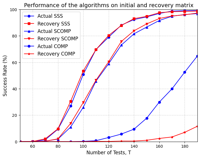
Figure 2: Performance of the COMP, SCOMP and SSS algorithms for the matrix $\mathbf{M}^{\blacksquare}$ after recovery (the recovery ones) compared to the measurement matrix $\mathbf{M}$ (the actual ones). Here, we use the noiseless group testing set up with a Bernoulli test design with $n=500,d=10,p=0.1$. Additionally, each cell is missing with probability 0.1 and $s=10$ samples are used to recover the missing matrix.

In this section, we conduct experiments to demonstrate that the performance of state-of-the-art algorithms (COMP, SCOMP, and SSS in [27]) for noiseless group testing remains consistent when applied to the recovery matrix (i.e., the matrix $\mathbf{M}^{\blacksquare}$ after recovering missing entries) compared to the measurement matrix $\mathbf{M}$. Specifically, our simulations are conducted with $n=500$ items, of which 10 are defective. The matrix $\mathbf{M}$ is generated using a Bernoulli test design with parameter $p=\frac{1}{d}=0.1$. Additionally, we set the probability of a cell in $\mathbf{M}$ being missing to 0.1. After creating the missing matrix $\mathbf{M}^{\blacksquare}$, we use $s=10$ samples (taken randomly) to solve the group testing problem consisting of the erased matrix $\Gamma$ and the erased vector $\mathbf{v}$. Finally, we plot the average success rate from 1,000 simulations for both the measurement matrix $\mathbf{M}$ and the matrix $\mathbf{M}^{\blacksquare}$ after recovery, for each algorithm, across a range of test numbers $t$ from 50 to 200.

Fig. 2 presents the results of our experiments. For both state-of-the-art algorithms, SSS and SCOMP, the performance on the measurement matrix and the recovered matrix is approximately the same, with the largest observed error being no more than 4%. However, for less accurate algorithms like COMP, the performance on the recovered matrix struggles to match that of the measurement matrix. This discrepancy arises due to inaccuracies in solving the group testing problem between the erased matrix and the erased vector.

VI Conclusion

We consider a variant of the matrix completion problem in group testing. Instead of using the rank of the measurement matrix to recover it from the missing matrix, we utilize a number of observed input and outcome vector. In particular, given the missing matrix $\mathbf{M}^{\blacksquare}$ and the number of input and outcome vectors observed, we construct an erased matrix $\Gamma$ and an erased vector $\mathbf{v}$ such that $\Gamma\odot\mathbf{\psi}=\mathbf{v}$ with no duplicated rows in $\Gamma$, where $\mathbf{\psi}$ is the representation vector of all missing entries in $\mathbf{M}^{\blacksquare}$. More importantly, we have shown that the information gain from erased matrix $\Gamma$ and erased vector $\mathbf{v}$ is equivalent to that of the missing matrix $\mathbf{M}^{\blacksquare}$ and the set of observed samples. Therefore, to reconstruct the measurement matrix, one only needs to reconstruct $\mathbf{\psi}$ from $\Gamma$ and $\mathbf{v}=\Gamma\odot\mathbf{\psi}$.

Since the more rows $\Gamma$ has, the better the chance we have of recovering $\mathbf{\psi}$, we derive the exact and approximate expected number of rows $\Gamma$. Unfortunately, in some cases, it is impossible to recover the missing entries regardless of the number of input and outcome vectors observed. This behavior should be studied in future.

Appendix A Illustration of Theorem 1

A-A Algorithm

The procedure in Theorem 1 can be parsed to Algorithm 1.

Algorithm 1 Construction of Erased Matrix $\Gamma$ and Erased Vector $\mathbf{v}$

1:Initialize an empty $0\times r$ matrix $\Gamma$ and a $0\times 1$ vector $\mathbf{v}$

2:for each pair $(\mathbf{x},i)\in\chi\times[t]$ that is informative do

3:  Initialize a row vector $\mathbf{g}$ of length $n$ with all zeros

4:  for each $z\in[n]$ do

5:   if $i_{z}=i$ and $\mathbf{x}_{j_{z}}=1$ then

6:     Set $g_{z}=1$

7:   else

8:     Set $g_{z}=0$

9:   end if

10:  end for

11:  Append row $\mathbf{g}$ to matrix $\Gamma$

12:  Append $y_{i}$ to vector $\mathbf{v}$

13:end for

14:Remove duplicate rows from $\Gamma$ and corresponding entries from $\mathbf{v}$

15:return $\Gamma$ and $\mathbf{v}$

A-B Feasible recovery

In this example, we show that it is feasible to recover all missing entries. Let us assume the measurement matrix $\mathbf{M}$ and its erased matrix $\mathbf{M}^{\blacksquare}$ are as in Eq. 1. By Theorem 1, the set $\psi=\{\psi_{1},\psi_{2},\psi_{3},\psi_{4},\psi_{5}\}$ is the solution to the group testing problem with the testing matrix being $\Gamma$ and the testing vector being $\mathbf{v}$. Now by solving $\Gamma$ and $\mathbf{v}$, we can recover the initial values of some of the missing entries of $\mathbf{M}$: $\psi_{3}=0,\psi_{4}=0,\psi_{5}=1.$

However, we do not have enough information to recover $\psi_{1},\psi_{2}$. To demonstrate that the larger the size of $\chi$ and $\gamma$, the more chance we will get at recovering the missing entries. Let us say another pair $(\mathbf{x}_{3},\mathbf{y}_{3})$ is added to $\chi\times\gamma$ where:

$$\begin{Bmatrix}\mathbf{x}_{3}=\left[0,1,1,0,0,0,0,0,0,0,0,0\right]^{T}&;&\mathbf{y}_{3}=[0,0,1,0,1,1,1,1,0]^{T}.\end{Bmatrix}$$

Then we get $(\mathbf{x}_{3},2)$ is informative. Hence our erased matrix and erased vector will be modified as follows:

$$\Gamma=\left[\begin{array}[]{ccccccc}1&1&0&0&0\\ 0&0&1&0&0\\ 0&0&0&0&1\\ 0&0&1&1&0\\ 1&0&0&0&0\end{array}\right],\mathbf{v}=\left[\begin{array}[]{c}0\\ 0\\ 1\\ 0\\ 0\end{array}\right]$$ (32)

By solving $\mathbf{v}=\Gamma\odot\psi$, we recover $\psi_{1}=0,\psi_{2}=1$. In summary, the missing values in $\overline{\Psi}=\{(2,3),(2,4),(5,3),(5,6),(6,4)\}$ are $0,1,0,0,1$, respectively.

A-C Infeasible recovery

In the example in Section A-C, by using our method and a sufficient amount of samples, we are able to recover the measurement matrix $\mathbf{M}$. However, in certain cases, even with a lot of samples, we are not able to fully recover $\mathbf{M}$. We will show this in our following example. Consider the matrix $\mathbf{M}$ defined in Eq. 1 and its missing matrix as follows:

$$\mathbf{M}^{\blacksquare}=\left[\begin{array}[]{cccccccccccc}0&\blacksquare&0&1&1&1&1&1&1&\blacksquare&1&1\\ 0&0&0&1&1&1&0&0&0&1&0&0\\ 1&1&1&0&0&0&0&0&0&1&0&0\\ 0&0&1&0&0&1&0&0&1&0&1&0\\ 0&1&0&0&1&0&0&1&0&0&1&0\\ 1&0&0&1&0&0&1&0&0&0&1&0\\ 0&1&0&0&0&0&1&0&1&0&0&1\\ 0&1&0&0&1&0&1&0&0&0&0&1\\ 1&0&0&0&0&1&0&1&0&0&0&1\end{array}\right].$$ (33)

Suppose we know that the number of defectives is $d=5$. Despite the fact that the matrix $\mathbf{M}$ has only two missing entries, it is impossible to recover them due to the overwhelming number of $1$ entries observed in their corresponding tests. Indeed, consider a sample $\mathbf{x}\in\chi$. Since $\mathbf{x}$ must contain at least 5 ones, and the row in $\mathbf{M}$ that includes both missing entries has at most entries that are not ones, none of the possible choices of $\mathbf{x}$ can yield informative results when paired with $(\mathbf{x},1)$. Consequently, the erased matrix $\Gamma$ remains empty regardless of the number of samples we collect. In this scenario, recovering $\mathbf{M}$ using only the current method is infeasible. Additional conditions or assumptions are required to achieve a solution.

References

- [1] R. Dorfman, “The detection of defective members of large populations,” The Annals of mathematical statistics, vol. 14, no. 4, pp. 436–440, 1943.
- [2] O. Sporns, “The human connectome: a complex network,” Annals of the new York Academy of Sciences, vol. 1224, no. 1, pp. 109–125, 2011.
- [3] S. Herculano-Houzel, “The remarkable, yet not extraordinary, human brain as a scaled-up primate brain and its associated cost,” Proceedings of the National Academy of Sciences, vol. 109, no. supplement_1, pp. 10661–10668, 2012.
- [4] C. Stringer, M. Pachitariu, N. Steinmetz, M. Carandini, and K. D. Harris, “High-dimensional geometry of population responses in visual cortex,” Nature, vol. 571, no. 7765, pp. 361–365, 2019.
- [5] C. Stringer, L. Zhong, A. Syeda, F. Du, M. Kesa, and M. Pachitariu, “Rastermap: a discovery method for neural population recordings,” Nature Neuroscience, pp. 1–12, 2024.
- [6] T. V. Bui, “A simple self-decoding model for neural coding,” in 2024 IEEE International Symposium on Information Theory (ISIT), pp. 268–273, IEEE, 2024.
- [7] S. L. Smith, I. T. Smith, T. Branco, and M. Häusser, “Dendritic spikes enhance stimulus selectivity in cortical neurons in vivo,” Nature, vol. 503, no. 7474, pp. 115–120, 2013.
- [8] G. Kastellakis, D. J. Cai, S. C. Mednick, A. J. Silva, and P. Poirazi, “Synaptic clustering within dendrites: an emerging theory of memory formation,” Progress in neurobiology, vol. 126, pp. 19–35, 2015.
- [9] W. C. Abraham, O. D. Jones, and D. L. Glanzman, “Is plasticity of synapses the mechanism of long-term memory storage?,” NPJ science of learning, vol. 4, no. 1, p. 9, 2019.
- [10] D. Du, F. K. Hwang, and F. Hwang, Combinatorial group testing and its applications, vol. 12. World Scientific, 2000.
- [11] A. D’yachkov, N. Polyanskii, V. Shchukin, and I. Vorobyev, “Separable codes for the symmetric multiple-access channel,” IEEE Transactions on Information Theory, vol. 65, no. 6, pp. 3738–3750, 2019.
- [12] N. Shental, S. Levy, V. Wuvshet, S. Skorniakov, B. Shalem, A. Ottolenghi, Y. Greenshpan, R. Steinberg, A. Edri, R. Gillis, et al., “Efficient high-throughput SARS-CoV-2 testing to detect asymptomatic carriers,” Science advances, vol. 6, no. 37, p. eabc5961, 2020.
- [13] W. Kautz and R. Singleton, “Nonrandom binary superimposed codes,” IEEE Transactions on Information Theory, vol. 10, no. 4, pp. 363–377, 1964.
- [14] A. G. D’yachkov and V. V. Rykov, “Bounds on the length of disjunctive codes,” Problemy Peredachi Informatsii, vol. 18, no. 3, pp. 7–13, 1982.
- [15] A. G. Dyachkov and V. V. Rykov, “A survey of superimposed code theory,” Problems of Control and Information Theory, vol. 12, no. 4, pp. 1–13, 1983.
- [16] E. Porat and A. Rothschild, “Explicit nonadaptive combinatorial group testing schemes,” IEEE Transactions on Information Theory, vol. 57, no. 12, pp. 7982–7989, 2011.
- [17] P. Indyk, H. Q. Ngo, and A. Rudra, “Efficiently decodable non-adaptive group testing,” in ACM-SIAM Symposium on Discrete Algorithms, pp. 1126–1142, SIAM, 2010.
- [18] H. Q. Ngo, E. Porat, and A. Rudra, “Efficiently decodable error-correcting list disjunct matrices and applications - (extended abstract),” in Automata, Languages and Programming - 38th International Colloquium, ICALP 2011, Zurich, Switzerland, July 4-8, 2011, Proceedings, Part I (L. Aceto, M. Henzinger, and J. Sgall, eds.), vol. 6755 of Lecture Notes in Computer Science, pp. 557–568, Springer, 2011.
- [19] M. Cheraghchi, “Noise-resilient group testing: Limitations and constructions,” Discrete Applied Mathematics, vol. 161, no. 1-2, pp. 81–95, 2013.
- [20] M. Cheraghchi and V. Nakos, “Combinatorial group testing and sparse recovery schemes with near-optimal decoding time,” in 2020 IEEE 61st Annual Symposium on Foundations of Computer Science (FOCS), pp. 1203–1213, IEEE, 2020.
- [21] A. De Bonis, L. Gasieniec, and U. Vaccaro, “Optimal two-stage algorithms for group testing problems,” SIAM Journal on Computing, vol. 34, no. 5, pp. 1253–1270, 2005.
- [22] J. Scarlett, “Noisy adaptive group testing: Bounds and algorithms,” IEEE Transactions on Information Theory, vol. 65, no. 6, pp. 3646–3661, 2018.
- [23] B. Teo and J. Scarlett, “Noisy adaptive group testing via noisy binary search,” IEEE Transactions on Information Theory, vol. 68, no. 5, pp. 3340–3353, 2022.
- [24] F. Hwang, “A generalized binomial group testing problem,” Journal of the American Statistical Association, vol. 70, no. 352, pp. 923–926, 1975.
- [25] M. Mézard and C. Toninelli, “Group testing with random pools: Optimal two-stage algorithms,” IEEE Transactions on Information Theory, vol. 57, no. 3, pp. 1736–1745, 2011.
- [26] M. Aldridge, “Conservative two-stage group testing,” arXiv preprint arXiv:2005.06617, 2020.
- [27] M. Aldridge, L. Baldassini, and O. Johnson, “Group testing algorithms: Bounds and simulations,” IEEE Transactions on Information Theory, vol. 60, no. 6, pp. 3671–3687, 2014.
- [28] J. Scarlett and V. Cevher, “Phase transitions in group testing,” in Proceedings of the twenty-seventh annual ACM-SIAM symposium on Discrete algorithms, pp. 40–53, SIAM, 2016.
- [29] M. Aldridge, O. Johnson, J. Scarlett, et al., “Group testing: an information theory perspective,” Foundations and Trends® in Communications and Information Theory, vol. 15, no. 3-4, pp. 196–392, 2019.
- [30] A. Coja-Oghlan, O. Gebhard, M. Hahn-Klimroth, and P. Loick, “Optimal group testing,” in Conference on Learning Theory, pp. 1374–1388, PMLR, 2020.
- [31] E. Price and J. Scarlett, “A fast binary splitting approach to non-adaptive group testing,” Approximation, Randomization, and Combinatorial Optimization. Algorithms and Techniques (APPROX/RANDOM 2020), 2020.
- [32] P. Damaschke, “Threshold group testing,” in General theory of information transfer and combinatorics, pp. 707–718, Springer, 2006.
- [33] N. H. Bshouty, “Optimal algorithms for the coin weighing problem with a spring scale.,” in COLT, vol. 2009, p. 82, 2009.
- [34] H.-B. Chen and H.-L. Fu, “Nonadaptive algorithms for threshold group testing,” Discrete Applied Mathematics, vol. 157, no. 7, pp. 1581–1585, 2009.
- [35] T. V. Bui and J. Scarlett, “Concomitant group testing,” IEEE Transactions on Information Theory, vol. 70, no. 10, pp. 7179–7192, 2024.
- [36] P. Nikolopoulos, S. R. Srinivasavaradhan, T. Guo, C. Fragouli, and S. N. Diggavi, “Community-aware group testing,” IEEE Transactions on Information Theory, vol. 69, no. 7, pp. 4361–4383, 2023.
- [37] N. ACM SIGKDD, “Proceedings of kdd cup and workshop,” in Proceedings of KDD Cup and Workshop, 2007.
- [38] E. Candes and B. Recht, “Exact matrix completion via convex optimization,” Communications of the ACM, vol. 55, no. 6, pp. 111–119, 2012.
- [39] R. H. Keshavan, A. Montanari, and S. Oh, “Matrix completion from a few entries,” IEEE transactions on information theory, vol. 56, no. 6, pp. 2980–2998, 2010.
- [40] E. J. Candès and T. Tao, “The power of convex relaxation: Near-optimal matrix completion,” IEEE transactions on information theory, vol. 56, no. 5, pp. 2053–2080, 2010.
- [41] B. Recht, “A simpler approach to matrix completion.,” Journal of Machine Learning Research, vol. 12, no. 12, 2011.
- [42] S. Bhojanapalli and P. Jain, “Universal matrix completion,” in International Conference on Machine Learning, pp. 1881–1889, PMLR, 2014.