An Efficient Diffusion-based Non-Autoregressive Solver for Traveling Salesman Problem

Abstract.

Recent advances in neural models have shown considerable promise in solving Traveling Salesman Problems (TSPs) without relying on much hand-crafted engineering. However, while non-autoregressive (NAR) approaches benefit from faster inference through parallelism, they typically deliver solutions of inferior quality compared to autoregressive ones. To enhance the solution quality while maintaining fast inference, we propose DEITSP, a diffusion model with efficient iterations tailored for TSP that operates in a NAR manner. Firstly, we introduce a one-step diffusion model that integrates the controlled discrete noise addition process with self-consistency enhancement, enabling optimal solution prediction through simultaneous denoising of multiple solutions. Secondly, we design a dual-modality graph transformer to bolster the extraction and fusion of features from node and edge modalities, while further accelerating the inference with fewer layers. Thirdly, we develop an efficient iterative strategy that alternates between adding and removing noise to improve exploration compared to previous diffusion methods. Additionally, we devise a scheduling framework to progressively refine the solution space by adjusting noise levels, facilitating a smooth search for optimal solutions. Extensive experiments on real-world and large-scale TSP instances demonstrate that DEITSP performs favorably against existing neural approaches in terms of solution quality, inference latency, and generalization ability. Our code is available at https://github.com/DEITSP/DEITSP.

1. Introduction

The Traveling Salesman Problem (TSP) is a well-known combinatorial optimization problem that formulated on a fully connected graph with non-negative edge weights (Garey and Johnson, 1990). A TSP solution manifests as a Hamiltonian cycle, where the objective is to minimize the sum of edge weights along the tour. In this context, a Hamiltonian cycle refers to a tour that starts and ends at the same node while visiting each remaining node exactly once. TSP has diverse applications in practical scenarios, such as transportation and facility location (Christiansen et al., 2004; Wu et al., 2023b). Given its significance in both theoretical and practical realms, numerous exact (Bellman, 1962; Padberg and Rinaldi, 1991; Applegate et al., 2007), approximate (Bansal et al., 2004; Kizilateş and Nuriyeva, 2013; Wu et al., 2023a), and heuristic algorithms (Helsgaun, 2017; Zhong et al., 2018; Onizawa et al., 2022) have emerged over the years. However, most of these algorithms are intricate, characterized by many manually formulated rules that heavily rely on expert knowledge.

In recent years, neural network (NN)-based models have emerged as a promising alternative for addressing the complexities of the TSP (Wu et al., 2024). Although these models lack well-established theoretical guarantees, empirical evidence suggests they can achieve near-optimal solutions. NN-based models for TSP can be broadly categorized into two types based on their decoding strategies: Autoregressive (AR) and Non-Autoregressive (NAR). AR models, inspired by neural machine translation, sequentially generate nodes on the Hamiltonian cycle and have shown satisfactory performance (Kool et al., 2019; Bresson and Laurent, 2021; Kim et al., 2021; Xin et al., 2021; Gao et al., 2023; Jung et al., 2023). However, their inherent sequential nature limits the inference speed of these networks. In contrast, NAR models generate solutions in a one-shot manner for fast inference.

While earlier NAR models often yield lower-quality solutions, recent advancements in diffusion-based learning for TSP have shown improvements in solution quality. Graikos et al. (2022) transformed TSP instances into low-resolution grayscale images using an image-based diffusion model. Sun and Yang (2023) developed a graph-based diffusion model to explicitly represent problems as graph. Ma and Dou (2024) proposed a semi-supervised training strategy for diffusion models, while Li et al. (2024) incorporated objective optimization guidance into the denoising steps through gradient feedback, enhancing sampling efficiency. Although these approaches improve performance, they often rely on simulating a Markov chain with numerous steps, which increases time overhead. Moreover, these methods tend to focus excessively on obtaining a single high-quality solution, often neglecting the exploration of the solution space, resulting in high computational costs for marginal improvements, especially when faced with test problems that differ in size and distribution from those seen during training.

To enhance generalization ability and inference speed, we propose an efficient diffusion model named DEITSP. This model directly maps noise to the optimal solution, eliminating the need for multi-step Markov processes. Unlike previous NAR approaches that generate only a single solution, DEITSP simultaneously explores multiple solutions. We introduce an efficient iterative strategy that alternates between adding and removing noise for generating multiple solutions to improve exploration and solution quality. Our approach provides flexibility by allowing users to adjust the number of iteration steps according to practical needs, balancing the trade-off between solution quality and inference speed. Specifically, DEITSP formulates the generation of adjacency matrices as edge classification tasks. Our model consists of three key components: (1) a one-step diffusion model based on a controlled discrete noise addition process and self-consistency enhancement, enabling high-quality solution prediction through single-step denoising; (2) a dual-modality graph transformer that enhances the extraction and integration of features from different modalities with fewer layers, achieving faster inference and stronger feature representation; and (3) an efficient iterative strategy that alternates between adding and removing noise to enhance exploration and refine the solution space of TSP, along with a corresponding scheduling framework that adjusts noise levels to facilitate a smooth search for solutions.

We conducted extensive experiments comparing DEITSP with 16 NN-based baselines on TSP instances ranging in size from 20 to 1000 nodes. DEITSP achieved the highest solution quality and demonstrated superior generalization, effectively scaling from small to large TSP instances. It also generalized well to instances beyond the training distribution, including real-world cases from the USA, Japan, Burma, and TSPLIB (Reinelt, 1991; Goh et al., 2024). Ablation experiments further confirmed the effectiveness of our proposed components.

We summarize our contributions as follows:

• We introduce a one-step diffusion model that enables optimal TSP solution prediction through simultaneous denoising of multiple solutions.

• We design a dual-modality graph transformer that significantly enhances feature extraction and fusion from node and edge modalities, resulting in faster inference and more robust feature representation.

• We develop an efficient iterative strategy specifically tailored for TSP, alternating between adding and removing noise to enhance exploration and progressively refine the solution space, thereby improving solution quality.

• We devise a scheduling framework to adjust noise levels automatically, facilitating a smooth optimal solution search.

• We validate DEITSP through extensive experiments, demonstrating its excellence in solution quality, inference speed, and generalization across various real-world TSP instances and large-scale benchmarks.

2. Related Work

In this section, we review NN-based TSP solvers, which are typically categorized as either AR or NAR based on decoding methods. We also introduce discrete diffusion models relevant to our work.

2.1. Neural Network-based TSP Solvers

With recent advancements in deep learning, numerous NN-based models have been proposed to solve TSPs. These models can be broadly categorized into AR and NAR based on their decoding methods. It is important to note that we focus on end-to-end learning methods for solving TSPs, excluding neural improvement algorithms that combine deep learning with heuristic search, as they typically result in longer inference latency.

We first review pioneering NN-based approaches for solving TSPs using AR decoding. Vinyals et al. (2015) proposed a sequence-to-sequence supervised learning (SL) model called Pointer Network (PtrNet), which uses the Long Short-Term Memory (LSTM) architecture from natural language processing (Bahdanau et al., 2015). PtrNet inputs node coordinates, employs an attention mechanism, and generates TSP solutions via supervised learning step-by-step. While PtrNet provides a novel perspective for solving Combinatorial Optimization (CO) problems, its unsatisfactory performance makes it challenging to be applied in practical settings (Li et al., 2021; Fu et al., 2021). Subsequently, Bello et al. (2017) expanded PtrNet with an actor-critic reinforcement learning (RL) algorithm, eliminating the need for optimal solutions during training. Nazari et al. (2018) further enhanced PtrNet’s performance with node embeddings from attention layer. Recently, the Transformer has set new performance records in various applications (Vaswani et al., 2017), leading to several Transformer-based TSP models, notably (Kool et al., 2019; Kwon et al., 2020; Bresson and Laurent, 2021; Deudon et al., 2018). Kim et al. (2022) improved generalization by leveraging symmetries like rotational and reflectional invariance. Jung et al. (2023) introduced a lightweight CNN-Transformer model using a CNN embedding layer and partial self-attention. Gao et al. (2023); Jiang et al. (2023b); Xiao et al. (2024b) integrated extra policies to enhance generalization. These models share the same Transformer-encoder architecture but differ in the decoder. Specifically, Deudon et al. (2018) used node information from the last three steps, Kool et al. (2019) used information from the first and last steps, Jiang et al. (2023a) employ contrastive learning to enhance the embedding of nodes, and Bresson and Laurent (2021) fused all previously output node information. All of these models demonstrate excellent performance.

However, the constructive methods used by AR models naturally disadvantage inference speed compared to NAR approaches (Ran et al., 2021; Sun and Yang, 2023). To address this issue, several NAR models have been developed to improve inference speed when solving TSPs (Nowak et al., 2018; Joshi et al., 2019). These models treat TSP as a link prediction task, which has been studied in various research fields (Wang et al., 2019; Xiao et al., 2020, 2023). They use supervised learning (SL) to train their models to estimate the importance of each edge in the optimal solution. For instance, Nowak et al. (2018); Joshi et al. (2019) utilized a graph network based TSP solver trained with SL, which takes a TSP instance as a graph input and directly outputs a heat map representing the importance of edges. It is worth noting that during training, these models relax the sequential constraint and obtain the edge’s importance prediction by minimizing the binary cross-entropy loss between the adjacency matrix of the optimal solution and their heat map. During inference, these models apply greedy search or beam search on the heat map to obtain a feasible TSP solution. Despite the significant improvement in inference speed offered by NAR approaches (Nowak et al., 2018; Xiao et al., 2023, 2024a), the solution quality of these models is often suboptimal. Existing NAR models generally fail to outperform most of the aforementioned AR models (Joshi et al., 2019, 2022; Xiao et al., 2023). Thus, there is a pressing need to further improve existing models to achieve high-quality solutions with low inference latency.

2.2. Diffusion Models

Discrete diffusion models (Song et al., 2020) operate in the discrete domain using noise distributions like Bernoulli in the forward process. These models transform the original data distribution into a noised distribution and then train neural networks to reverse this process. They have been effectively applied in graph structure generation (Vignac et al., 2023), image generation (Song et al., 2020), and improved text generation (Chen et al., 2023). However, their sampling processes require numerous iterations , which typically results in slow speeds. To address this issue, Song et al. (2023) introduced the consistency model, which uses consistency mapping to achieve rapid one-step generation by directly mapping any state in the noise trajectory to its origin.

Recent studies have explored the use of diffusion-based generative models to solve TSP. Graikos et al. (2022) extended the diffusion model for image generation to the Euclidean TSP by generating a 64x64 grayscale image to represent the solution of the TSP instance, which is then decoded into a TSP tour. This image-based method is limited as it cannot explicitly model the node/edge selection process, resulting in suboptimal solution quality and increased inference delay. Sun and Yang (2023) reformulated the TSP as a discrete {0,1} vector optimization problem and utilized a graph-based denoising diffusion model to generate TSP solutions represented by adjacency matrices. Ma and Dou (2024) proposed a diffusion model training strategy in a semi-supervised manner. Li et al. (2024) incorporated objective optimization guidance into the denoising steps through gradient feedback for more efficient sampling. Although these approaches demonstrate improved performance, they rely on the standard DDIM paradigm (Song et al., 2020), which necessitates simulating a Markov chain with a substantial number of steps for generation, significantly increasing time overhead. This limitation deprives them of the speed advantage of NAR approaches and hinders their practicality in time-sensitive real-world applications (Xu et al., 2018). In contrast, DEITSP directly maps noise to the optimal solution by enhancing self-consistency (Song et al., 2023) and develops a specialized iteration process tailored for TSP, which contributes to improved efficiency in both inference speed and solution quality. Additionally, DEITSP offers the flexibility to balance solution quality and inference speed by allowing users to choose the number of iteration steps.

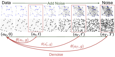
Figure 1. The proposed diffusion model learns to directly map any state in the noise trajectory to its origin state (i.e. the optimal solution), where $\theta$ denotes the neural network and $g$ represents the TSP instance as the condition.

The proposed consistency model learns to directly map any time point in the noise trajectory to its origin time point.

3. Methodology

In this section, we introduce DEITSP, our diffusion-based NAR model designed to efficiently generate high-quality TSP solutions with minimal iteration steps. In Section 3.2, we present a one-step diffusion model that combines a controlled discrete noise addition process with self-consistency enhancement, allowing predicting optimal solutions through single-step denoising from various noise data. Section 3.3 details a dual-modality graph transformer, which enhances the extraction and fusion of features from different modalities. Finally, in Section 3.4, we describe an efficient iterative strategy that leverages the network’s denoising ability at different noise levels, progressively compressing the solution space, enhancing exploration capabilities, and iteratively improving solution quality, without following the standard DDIM paradigm (Song et al., 2020).

3.1. TSP Setting

Our research focuses on the two-dimensional Euclidean TSP, widely used and highly significant in various domains. We represent the TSP instance as a graph $g=\left(V,A\right)$ where $V=\{v_{i}|1\leq i\leq N\}$ denotes all $N$ node coordinates and $A=\{a_{ij}|1\leq i,j\leq N\}$ denotes the connectivity between nodes. The connected edges form a Hamiltonian loop that visits each node in $V$ exactly once. The cost of feasible solutions is defined as: $\mathrm{L}(A)={\textstyle\sum_{i}\textstyle\sum_{j}a_{ij}\times\mathrm{cost}(v_{i},v_{j})}$, where $\mathrm{cost}(v_{i},v_{j})$ represents the Euclidean distance between $v_{i}$ and $v_{j}$, and $\mathrm{L}(\cdot)$ denotes the length of the TSP solution. For a given TSP instance $s$, our goal is to find the optimal solution that minimizes the cost among feasible ones:

(1) $$A^{*}=\mathrm{arg}\min_{A\in\mathcal{A}}\mathrm{L}(A).$$

3.2. One-step Diffusion Model

In this subsection, we first introduce the parameterization of the controlled discrete noise addition process. Next, we describe the self-consistency enhancement during the training process, enabling direct prediction of high-quality solutions through single-step denoising from various noise levels.

3.2.1. Controlled Discrete Noise Addition

We design a diffusion model based on the discrete diffusion model (Austin et al., 2021) and consistency model (Song et al., 2023) to support a controllable process for disturbing TSP solutions with varying noise levels. Similar to image-based diffusion models treating each pixel as data, we consider each edge’s connectivity as data following the Bernoulli distribution. Given the optimal solution $A_{0}$, each edge is represented by a one-hot row vector $a_{0}\in{0,1}$.

The noise addition process is determined by the transition matrix $\left[\mathbf{Q_{t}}\right]_{ss^{\prime}}={q}(a_{t}=s^{\prime}|a_{t-1}=s)$, where $\left[\mathbf{Q_{t}}\right]_{ss^{\prime}}$ represents the probability of transition from state $s$ to state $s^{\prime}$ and $t$ represents the noise level. For any edge, the noise addition process is defined as:

(2) $${q}(a_{t}|a_{0})=\mathrm{Cate}(a_{t};\boldsymbol{p}=a_{0}\mathbf{\overline{Q}_{t}}),$$

where $\mathbf{\overline{Q}_{t}}=\mathbf{Q_{1}}\mathbf{Q_{2}}...\mathbf{Q_{t}}$ and $\mathrm{Cate}(a;p)$ is a categorical distribution over the one-hot row vector $a$ with probabilities $p$ to add noise to disturb an edge. We parameterize the probability transition matrix as $\mathbf{Q_{t}}=\begin{bmatrix}(1-\beta_{t})&\beta_{t}\\ \beta_{t}&(1-\beta-t)\end{bmatrix}$ following (Austin et al., 2021). The diffusion rates $\beta_{t}$ should be defined such that $\prod_{t=1}^{T}(1-\beta_{t})\approx 0$, ensuring ${q}(a_{T}|a_{0})$ to converge to a uniform distribution independent of $a_{0}$, i.e., ${q}(a_{t}|a_{0})\approx{Uniform}(a_{t})$. We set $\beta_{t}$ to follow a linear schedule starting from $\beta_{1}=10^{-4}$ and ending at $\beta_{T}=0.02$ as described in (Ho et al., 2020; Graikos et al., 2022).

Algorithm 1 Training DEITSP

1: Input: dataset D, initial model parameter $\theta$.

2: repeat

3:  $a_{0},g\sim D$. $\triangleright$ Get TSP instance $g$ and ground truth $a_{0}$

4:  $t\sim\operatorname{Uniform}(\{1,\ldots,T\})$.

5:  $a_{t}\sim Cate(a_{t};p=a_{0}\bar{Q_{t}})$. $\triangleright$ Denoise

6:  $a_{t+k}\sim Cate(a_{t+k};p=a_{0}\bar{Q}_{t+k})$. $\triangleright$ Denoise from another noise level

7:  $\textrm{Minimize }\mathcal{L}(a_{0},\theta(a_{t},g),\theta(a_{t+k},g)$.

8: until convergence

3.2.2. Self-consistency Enhancement

The neural network $\theta$ is trained to directly predict the probability distribution of the optimal solution, namely $\tilde{a}_{0}$, also known as heatmap scores (Joshi et al., 2019; Sun and Yang, 2023). To facilitate the neural network’s learning for one-step denoising, we employ self-consistency (Song et al., 2023) to enhance the training process. As proposed by consistency models (Song et al., 2023), self-consistency ensures that all states along a noise trajectory map back to the same original state, as illustrated in Figure 1. This method imposes two key constraints: first, at any state on the noise trajectory, the denoising output generated by the neural network $\theta$ must be consistent with the ground truth, i.e., $\theta(a_{t},g)=a_{0}$ for all $t\in[1,{T}]$, where $g$ represents the input TSP instance as the condition. Second, the denoising outputs from any two states along the noise trajectory must be consistent with each other, i.e., $\theta(a_{t_{1}},g)=\theta(a_{t_{2}},g)$ for all $t_{1}$, $t_{2}\in[1,{T}]$.

3.2.3. Training Process

We optimize the model through supervised learning, with the ground truth $a_{0}$ obtained by the exact solver Concorde (Applegate et al., 2007). We add various levels of noise to the ground truth to obtain noisy data $a_{t},a_{t}^{\prime}$, and input them into the neural network to predict the denoised data $\tilde{a}_{0}$, $\tilde{a}_{0}^{\prime}$’. Then we train the model parameters end-to-end by minimizing the loss via gradient descent. The loss function, defined as Eq. (3), comprises three terms: the first two terms ensure the network’s output is consistent with the ground truth, while the third term enforces self-consistency between any two states on the noise trajectory. A parameter $\lambda$ balances these objectives. The overall training process of DEITSP is outlined in Algorithm 1. To stabilize training, the loss function ensures consistency not between any time steps, but between two intervals of $k$ steps, i.e., $a_{t+k}$ and $a_{t}$. Following (Luo et al., 2023), we set $k=20$.

$$\mathcal{L}=~ \mathrm{CrossEntropy}(a_{0},\theta(a_{t+k},g))+\mathrm{CrossEntropy}(a_{0},\theta(a_{t},g))$$

(3) $$+\lambda\cdot||\theta(a_{t+k},g)-\theta(a_{t},g)||_{2}.$$

3.3. Dual-modality Graph Transformer

In this section, we describe the three key components of our proposed dual-modality graph transformer. Existing methods (Joshi et al., 2019; Fu et al., 2021; Sun and Yang, 2023) typically utilize the anisotropic graph neural network with edge-gating mechanisms to extract latent features of the TSP through local aggregation. But their limited receptive field hinders the full exploitation of available data and restricts network depth, leading to slow inference speeds, particularly during multi-step denoising iterations. Moreover, deep GNNs suffer from excessive smoothing due to repeated local aggregation (Hussain et al., 2022).

To address these limitations, we design a dual-modality network based on the attention mechanism for continuous modes of nodes and discrete modes of edge links. Unlike neighborhood aggregation in conventional graph neural networks, the attention mechanism allows multi-hop interactions, thereby capturing a broader scope of structural information and reducing dependence on neural network depth. The personalized information of nodes is retained by applying different attention weights, which reduces the risk of node representations becoming overly similar. wu2024demystifying also indicates that the attention mechanism demonstrate slower rates of oversmoothing compared to GCNs. The backbone of DEITSP (Figure 2) consists of three key components: 1) a linear layer for input embedding; 2) multiple dual-modal learning layers for facilitating information transfer among nodes and edges; and 3) several classification layers for outputting edge scores.

3.3.1. Input Layer

For the given TSP instance $g=(V,A_{t})$, $A_{t}=\{a_{t_{ij}}|1\leq i,j\leq N\}$ represents the noisy adjacency matrix and $V=\{v_{i}|1\leq i\leq N\}$ represents the node coordinates. DEITSP linearly projects each input node $v_{i}$, edge $a_{t_{ij}}$, and time step $t$ that indicates noise level into $d$-dimensional hidden features. Their initial embedding is computed as follows:

$$h_{i}^{0}= \mathbf{W_{v}}v_{i}+\mathbf{b_{v}}+\mathrm{PE},$$

(4) $$x_{ij}^{0}= \mathbf{W_{a}}a_{t_{ij}}+\mathbf{b_{a}}+\mathrm{PE},$$

$$\hat{t}= \mathbf{W_{t}}t+\mathbf{b_{t}}+\mathrm{PE},$$

where $\mathbf{W_{v}}$, $\mathbf{W_{a}}$ and $\mathbf{b_{v}},\mathbf{b_{a}},\mathbf{b_{t}}$ are the parameters of the linear projection layers, and PE is the positional encoding (Vaswani et al., 2017).

3.3.2. Dual-modal Learning (DML) Layer

DEITSP utilizes $N$ dual-modal learning layer to extract information from TSP instances and maintain the features of nodes and edges at each layer. Edge features represent discrete adjacency relationships, while node features represent continuous node aggregation. Considering different modalities, we conducted separate feature extraction and mixing.

For nodes, we first use a mixing module to integrate edge features $x_{ij}^{l}$ into the implicit edge scores $\hat{w}_{ij}^{l}$ calculated from paired attention between nodes as in Eq. (5). Secondly, we use the scores $w_{ij}^{l}$ combining edge features to aggregate node features as in Eq. (6), and transmit them to the normalization layer, feedforward network, and residual connection to update node features as in Eq. (7).

(5) $$w_{ij}^{l}= \mathbf{W_{e_{1}}}x_{ij}^{l}\odot{}\hat{w}_{ij}^{l}+\mathbf{W_{e_{2}}}x_{ij}^{l}+\hat{w}_{ij}^{l},$$

(6) $$\hat{h}_{i}^{l+1}= \mathrm{softmax}({w_{ij}^{l}})\times{}\mathbf{V^{l}}h_{j},$$

(7) $$h_{i}^{l+1}= \mathbf{W_{h_{2}}}(\text{ReLU}(\mathbf{W_{h_{1}}}(\mathrm{Norm}(\hat{h}_{i}^{l+1}))))+h_{i}^{l},$$

where $l$ is the layer index and $V^{l}$ represents the weight for calculating attention at each layer. $\hat{w}_{ij}^{l}=(\frac{\mathbf{Q^{l}}h_{i}^{l}(\mathbf{K^{l}}h_{j}^{l})^{T}}{\sqrt{d}})$ represents the implicit edge scores calculated from paired attention between nodes.

For edges, we first use a mixing module to fuse the implicit edge scores $\hat{w}_{ij}^{l}$ into edge features $x_{ij}^{l}$ as in Eq. (8). The mixing modules of node and edge operate independently, distinguishing from typical graph transformers. Secondly, we combine time step features $\hat{t}$ with the mixed edge features $\hat{x}_{ij}^{l}$ as in Eq. (9), and pass them through the normalization layer, feedforward network, and residual connection to update edge features in Eq. (10) as:

(8) $$\hat{x}_{ij}^{l+1}= \mathbf{W_{y_{1}}}\hat{w}_{ij}^{l}\odot{}x_{ij}^{l}+\mathbf{W_{y_{2}}}\hat{w}_{ij}^{l}+x_{ij}^{l},$$

(9) $$\hat{x}_{ij}^{l+1}= \hat{x}_{ij}^{l+1}+\text{MLP}(\hat{t}),$$

(10) $$x_{ij}^{l+1}= \mathbf{W_{x_{2}}}(\text{ReLU}(\mathbf{W_{x_{1}}}(\mathrm{Norm}(\hat{x}_{ij}^{l+1}))))+x_{ij}^{l}.$$

where $l$ is the layer index and $\text{MLP}(\hat{t})=\mathbf{W_{t}^{l}}(\alpha(\hat{t}))$.

3.3.3. Classifier Layer

The classifier layer takes the edge embedding $x_{ij}^{N+1}$ of the last layer as input to predicts the heatmaps $\tilde{a}_{0_{ij}}$ of the optimal solution as follows:

(11) $$\tilde{a}_{0_{ij}}=\mathrm{Conv1d}(\alpha(\mathrm{Conv1d}(\mathrm{GN}(x_{ij}^{N+1})))),$$

where $\mathrm{Conv1d}$ is 1-d convolution, $\mathrm{GN}$ is the group normalization and $\alpha$ is the sigmoid activation function.

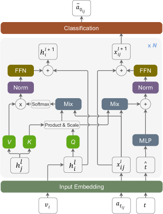
Figure 2. The network takes node coordinates $v_{i}$, noisy adjacency matrix $a_{t_{ij}}$ and time step $t$ as inputs to predicts the heatmaps $\tilde{a}_{0_{ij}}$. Mix refers to Eq. (5) and (8), while FFN and Norm is Feed Forward and Layer Normalization used in Vaswani et al. (2017)

The parametrization of our proposed graph transformer.

3.4. Iterative Denoising and Noise Scheduling

In this section, we present the inference process of DEITSP. First, we use a greedy strategy to decode the heatmaps predicted by neural networks into feasible TSP tours. A specific introduction to the decoding strategy is provided in Appendix A. Second, we propose an efficient iterative strategy that leverages denoising at different noise levels to enhance exploration. Finally, we design a novel schedule to control the level of noise addition during iterations, thereby gradually refining the solution space.

3.4.1. Iterative Strategy to Enhance Exploration

Unlike image generation, which has no fixed optimal solution, TSP has well-defined optimal solutions, making deviations during denoising less tolerable. The large solution space also complicates finding the optimal solution. Existing diffusion-based methods that employ the DDIM paradigm (Song et al., 2020) aim for a single high-quality solution through many generation steps. However, given the specific nature of TSP, which requires precise solutions and efficient exploration of a large solution space, previous approaches may not be effective for TSP.

Algorithm 2 DEITSP Inference

1: Input: Diffusion model $\theta$, noise schedule $\tau_{i}$, iteration step $M$, TSP instance $g$.

2: $a_{t}\sim\operatorname{Uniform}(a_{t}),\;t=T$ $\triangleright$ Generate initial solution

3: for $1$ to $M$  do

4:  $\tilde{a_{0}}=\theta(a_{t},g)$. $\triangleright$ One step denoising

5:  $\tilde{A_{0}}\leftarrow\tilde{a_{0}}$ $\triangleright$ Aggregate to solutions set

6:  $t=\tau_{i}$

7:  $a_{t}\sim\mathrm{Cate}(a_{t};p=a_{0}\mathbf{\overline{Q}_{t}})$ $\triangleright$ Adding noise

8: end for

9: ${a_{0}}^{*}=\arg\min_{\tilde{a_{0}}}(\text{GreedyDecoding}(\tilde{A_{0}}))$ $\triangleright$ Get the best solution from solutions set

10: Output: ${a_{0}}^{*}$

Different from the image generation task, which is challenging to achieve through single-step prediction, existing NAR models (Joshi et al., 2019; Xiao et al., 2023) have demonstrated the ability to effectively learn the latent representation of TSP solutions through single-step prediction. Consequently, we design a one-step diffusion model that directly maps noise to high-quality solutions through single-step denoising, bypassing the need for multi-step Markov processes.

Additionally, to reduce errors, DEITSP does not limit itself to a single high-quality solution but instead explores multiple solutions. We design an iterative strategy that alternates between adding and removing noise to enhance exploration. As shown in Figure 3, we add noise to the denoised data from the previous time step and denoise it again, leveraging different noise levels to obtain new results. We then aggregate the results $\{\tilde{a}_{0}^{t}\mid t\in[1,T]\}$ and decode all of them using greedy decoding to generate multiple solutions. This differs from the typical DDIM approach, where previously estimated results like $a_{t}$ are discarded when estimating $a_{t-1}$ at a new time step. Our iteration process fully utilizes the outputs from all iteration steps, exploring more high-quality solutions with minimal extra decoding cost. Moreover, unlike multiple sampling, where the inputs for each iteration are randomly generated, our method confines the exploration to relevant local regions of denoising data $\{\tilde{a}_{0}^{t}\mid t\in[1,T]\}$, improving the efficiency of the exploration. Notice that DEITSP is flexible to generate solutions from a single time step ($T=1$) or multiple time steps ($T>1$).

Table 1. Performance of DEITSP with comparisons with benchmarking methods on TSP20, TSP50 and TSP100.

Methods	Type	TSP20			TSP50			TSP100
		Len	Gap(%)	Time	Len	Gap(%)	Time	Len	Gap(%)	Time
Concorde	Exact	3.84	0.00	-	5.69	0.00	-	7.76	0.00	-
2 opt	Heuristic	3.94	2.51	8.41s	6.02	5.89	24.54s	8.35	7.61	53.74s
GAT*	NI, S, 2OPT	3.84	0.09	6m	5.75	1.00	32m	8.12	4.64	5h
DACT(1k Iter)	NI, G	3.84	0.01	17.86s	5.69	0.11	43.38s	7.89	1.62	1.75m
AM	AR, BS1280	3.84	0.00	32.17s	5.70	0.25	1.44m	7.95	2.44	3.61m
TRANSFORMER†	AR, BS1000	3.85	0.09	46.24s	5.69	0.02	2.89m	7.80	0.46	7.49m
MDAM	AR, G	3.86	0.57	4.69m	5.78	1.56	13.68m	7.99	2.99	20.38m
LCP(20 Iter)	AR, S1280	3.84	0.00	16.69m	5.69	0.02	23.95m	7.80	0.55	43.43m
POMO	AR, G, AUG	3.84	0.00	21.71s	5.69	0.09	44.84s	7.77	0.19	1.26m
Sym-NCO	AR, G, AUG	3.85	0.08	22.44s	5.69	0.04	45.97s	7.77	0.18	1.79m
CNN_Transformer†	AR, BS1000	3.85	0.28	50.01s	5.69	0.10	3.39m	7.85	1.13	9.99m
Pointerformer	AR, G, AUG	3.84	0.01	38.58s	5.69	0.10	1.35m	7.77	0.12	2.29m
ELG†	AR, G, AUG	3.85	0.10	55.22s	5.69	0.07	2.18m	7.77	0.20	4.14m
HierTSP	AR, G, AUG	3.84	0.00	33.48s	5.69	0.03	1.92m	7.78	0.21	2.79m
GCN	NAR, BS1280	3.87	0.80	27.40s	5.72	0.53	55.62s	7.96	2.53	1.78m
NAR4TSP†	NAR, BS1000	3.85	0.29	16.36s	5.70	0.25	27.21s	7.82	0.81	44.15s
Image Diffusion*	NAR, G, 2OPT	-	-	-	5.76	1.23	-	7.92	2.11	-
DIFUSCO†	NAR, G, 2OPT	3.85	0.19	6.88m	5.69	0.09	7.56m	7.78	0.23	9.47m
T2TCO†	NAR, G,2OPT	3.84	0.05	11.18m	5.69	0.02	24.91m	7.77	0.13	26.46m
DEITSP(1 Iter)	NAR, G, 2OPT	3.84	0.01	10.40s	5.70	0.12	15.05s	7.81	0.63	30.82s
DEITSP(4 Iter)	NAR, G, 2OPT	3.84	0.00	27.48s	5.69	0.03	32.37s	7.78	0.21	1.13m
DEITSP(16 Iter)	NAR, G, 2OPT	3.84	0.00	1.63m	5.69	0.01	1.99m	7.77	0.10	3.99m
G, S, BS, 2OPT, and AUG represent Greedy-search, Sampling, Beam-search, 2-opt process, and instance augmentation, respectively. * denotes baseline results from the original paper. †  indicates testing on TSP20/50 using pre-trained TSP50 weights provided by the original paper. Bold indicates the best solution; underlined indicates the second-best solution.

3.4.2. Noise Schedule to Refine the Solution Space

The level of noise added in each iteration affects both the exploration range and the solution space of the denoising process. Higher noise levels increase the exploration range but also introduce errors in network prediction. To balance this, we adopt a decreasing noise addition schedule that enhances exploration while gradually refining the solution space. Formally, we define the level of noise $\tau$ added in each iteration as a descending sequence within the range from $T$ to $1$. The setting of $\tau$ can be flexible, such as the commonly used linear schedule $\tau_{i}=\lfloor c_{i}\times T\rfloor$ for $c_{i}$ with uniform values in [0,1], or the cosine schedule $\tau_{i}=\lfloor\mathrm{cos}(\frac{(1-c_{i})\pi}{2})\times T\rfloor$ for $c_{i}$ with uniform values in [0,1]. A more general definition can also be employed:

(12) $$\tau_{i}=\left\lfloor(\frac{f(c_{i})-\mathrm{min}(f(c_{i}))}{\mathrm{max}(f(c_{i}))-\mathrm{min}(f(c_{i}))})\times T\right\rfloor,$$

where $f(\cdot)$ represents any elementary function, and $c_{i}$ can be uniformly distributed over any interval $[l,r]$. In this paper, we use the inverse function as $f(\cdot)$, with $c_{i}$ uniformly distributed in the interval $[0.25,1.5]$. This choice is motivated by the sparsity of the optimal solution, which leads to a significant difference in the distribution between the high-noise state and the optimal solution. Therefore, unlike the linear and cosine schedules typically used in image generations, the TSP requires more iterations in low-noise states. We present experiments on scheduling methods to verify this in Section 4.5 and provide detailed comparisons in Appendix B.

Algorithm 2 outlines the overall inference process of DEITSP. The initial solution $a_{t}$ is sampled from a uniform distribution $Uniform(a_{t})$ at time step $t=T$ (Step 2) and then input into the diffusion model $\theta$ to remove noise and predict the heatmaps $\tilde{a}_{0}$ of the optimal solution (Steps 4 and 5). Multiple solutions are then obtained by alternately adding and removing noise, with the noise schedule $\tau_{i}$ controlling the level of noise added in each step (Steps 6 and 7). Finally, we employ a greedy decoding method to produce the solutions from all steps and select the highest-quality solution (Steps 9 and 10).

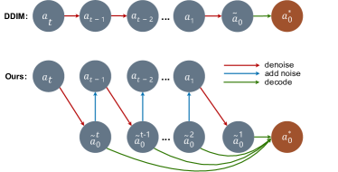
Figure 3. DDIM iteratively predicts $a_{t-1}$ to progress the chain of mapping noise into data, discarding previously estimated $\tilde{a_{0}}$. In contrast, our method aggregates the outputs of the diffusion model at multiple steps and decodes all outputs $\tilde{a}_{0}^{t}$ to improve solution quality.

Our method aggregates the outputs of multiple steps and decodes all outputs instead of the last one to explore higher-quality solutions.

4. Experiments

This section presents comprehensive evaluations of DEITSP. We begin by outlining the experimental settings, including benchmark datasets and baseline models. Then, we compare DEITSP’s performance with baseline models in solution quality and inference efficiency. Next, we assess DEITSP’s generalization capability across TSPs of varying sizes and distributions. Finally, we conduct ablation studies to examine the contributions of DEITSP’s components.

Table 2. Generalization performance of applying models trained using TSP100 on TSP200, TSP500 and TSP1000.

Methods	Type	TSP200			TSP500			TSP1000
		Len	Gap(%)	Time	Len	Gap(%)	Time	Len	Gap(%)	Time
Concorde	Exact	10.72	0.00	3.44m	16.55	0.00	37.66m	23.12	0.00	6.65h
GAT*	S, 2OPT	11.61	8.32	9.59m	23.75	43.57	57.76m	47.73	106.46	5.39h
GCN	BS1280	16.19	51.02	4.63m	30.37	83.55	38.02m	51.26	121.73	51.67m
AM	BS1280	11.38	6.14	5.77m	19.53	18.03	21.99m	29.90	29.24	1.64h
TRANSFORMER	BS2500	11.14	3.96	5.66m	20.77	25.55	34.30m	33.29	44.00	2.23h
POMO	G, AUG	10.89	1.64	20.48s	19.52	17.98	1.33m	30.51	31.96	8.80m
Sym-NCO	G, AUG	10.90	1.64	20.14s	19.84	19.93	1.35m	31.47	36.13	8.88m
Att-GCN*	MCTS	10.81	0.88	2.50m	16.97	2.54	5.91m	23.86	3.22	12.47m
DIFUSCO	G, 2OPT	10.81	0.78	2.98m	17.13	3.51	17.28m	24.25	4.89	1.15h
T2TCO	G,2OPT	10.78	0.55	6.18m	17.01	2.78	38.40m	OOM	OOM	OOM
Pointerformer	G, AUG	10.87	1.45	26.49s	18.62	12.53	1.35m	27.89	20.66	6.89m
ELG	G, AUG	10.90	1.64	46.64s	17.73	7.16	1.94m	25.74	11.36	3.99m
HierTSP	G, AUG	10.96	2.23	24.93s	18.54	12.08	1.50m	28.39	22.79	9.43m
BQ-NCO	G	11.20	4.51	2.52m	17.21	4.02	7.05m	24.09	4.19	23.43m
DEITSP(1 Iter)	G, 2OPT	10.89	1.52	11.40s	17.06	3.12	53.70s	24.14	4.41	3.77m
DEITSP(4 Iter)	G, 2OPT	10.80	0.70	24.80s	16.96	2.51	2.55m	24.06	4.07	11.24m
DEITSP(16 Iter)	G, 2OPT	10.77	0.40	1.41m	16.90	2.15	9.31m	23.97	3.68	41.83m
Bold indicates the best solution; underlined indicates the second-best solution.

4.1. Experiment Configurations

Dataset The training instances for TSP-20/50/100 are identical to those used in previous studies (Kool et al., 2019; Kwon et al., 2020; Joshi et al., 2022), where instances are uniformly generated within the range $[0,1]$. We generate the same test instances as (Joshi et al., 2022) for TSP-20/50/100 and as (Fu et al., 2021) for TSP-200/500/1000. To verify the generalization performance on realistic data, we sample instances from city maps of three different real-world countries, namely USA13509, BM33708 and JA9847 (Goh et al., 2024), as well as TSPLIB (Reinelt, 1991). We randomly sample problems of size 100 from the countries map. The optimal solution of testing instances are attained via Concorde (Applegate et al., 2007).

Baselines We conduct extensive comparisons of DEITSP against various baselines, including the exact solver Concorde (Applegate et al., 2007), heuristic method 2-opt (Lin and Kernighan, 1973), and several state-of-the-art learning-based approaches. The learning-based methods evaluated are categorized into three recent advancements: neural improvement methods, AR methods, and NAR methods. For neural improvement methods, we compare DEITSP with GAT (Deudon et al., 2018) and DACT (Ma et al., 2021). For AR methods, the baselines include AM (Kool et al., 2019), Transformer (Bresson and Laurent, 2021), MDAM (Kim et al., 2021), LCP (Xin et al., 2021), POMO (Kwon et al., 2020), Sym NCO (Kim et al., 2022), CNN_Transformer (Jung et al., 2023), Pointerformer (Jin et al., 2023), ELG (Gao et al., 2023), BQ-NCO (drakulic2024bq), and HierTSP (Goh et al., 2024). For NAR methods, we compare DEITSP with GCN (Joshi et al., 2019), Att-GCN (Fu et al., 2021), NAR4TSP (Xiao et al., 2023), and diffusion-based approaches such as Image Diffusion (Graikos et al., 2022), DIFUSCO (Sun and Yang, 2023), and T2TCO (Li et al., 2024). We use three key metrics for evaluation: average tour length (Len), average relative performance gap to Concorde (Gap), and total run time (Time).

Model Setting We use the same hyperparameters for DEITSP across all experiments. The graph transformer includes 6 dual-modal learning layers, each with a hidden dimension of 256 and 8 attention heads. For noise addition, we set $T=1000$ with a linear noise schedule for ${\beta}_{t}$ where $\beta_{1}={10}^{-4}$ and $\beta_{T}=0.02$. During inference, we use an inverse function iteration schedule, focusing on 1, 4, and 16 iteration steps. To ensure fair comparison, all NN-based models use the same batch size, with other settings following their defaults. All experiments are conducted on a system with an Intel Xeon Gold 6254 CPU and an NVIDIA RTX 3090 GPU. Our code and datasets will be publicly available.

Table 3. Generalization performance of applying models trained using TSP100 instances onto real-world instances.

Methods	JA9857			BM33708			USA13509			TSPLIB
	Len	Gap(%)	Time	Len	Gap(%)	Time	Len	Gap(%)	Time	Len	Gap(%)	Time
Concorde	78504.28	0.00	-	64760.71	0.00	-	2113007.65	0.00	-	31466.12	0.00	-
AM	506106.19	544.69	3.50m	283475.19	337.73	3.51m	10344162.00	389.55	3.58m	32704.00	3.93	13.15s
POMO	86095.99	9.67	1.27m	67152.81	3.69	1.31m	2252997.26	6.63	1.29m	31902.33	1.39	2.91s
Sym-NCO	86011.14	9.56	1.79m	66326.07	2.42	1.89m	2234747.53	5.76	1.85m	32069.48	1.92	2.98s
DIFUSCO	80360.48	2.36	9.53m	67862.36	4.79	9.47m	2202552.75	4.24	9.49m	31870.25	1.28	20.56s
T2TCO	79465.05	1.22	26.48m	66259.21	2.31	26.52m	2159342.20	2.19	26.46m	31750.49	0.90	28.96s
ELG	82528.93	5.13	4.14m	65765.26	1.55	4.21m	2158436.50	2.15	4.17m	31825.52	1.14	6.74s
HierTSP	84640.31	7.82	2.79m	66375.73	2.49	2.97m	2157443.98	2.10	3.58m	32025.60	1.78	3.86s
DEITSP(1 Iter)	80222.46	2.19	31.83s	67793.80	4.68	32.25s	2199481.21	4.09	35.42s	32000.50	1.70	2.61s
DEITSP(4 Iter)	79656.97	1.47	1.18m	67010.29	3.47	1.15m	2175058.13	2.94	1.22m	31777.83	0.99	4.82s
DEITSP(16 Iter)	79173.08	0.85	4.03m	66249.02	2.30	3.99m	2152979.27	1.89	4.11m	31711.94	0.78	8.51s
Bold indicates the best solution; underlined indicates the second-best solution.

4.2. Performance Comparison

Table 1 highlights the superior performance of DEITSP in both solution quality and inference speed. Specifically, with 16 iteration steps, DEITSP achieves results with minimal gaps to the optimal solutions produced by the exact algorithm Concorde. Compared to diffusion-based models like T2TCO (Li et al., 2024) and DIFUSCO (Sun and Yang, 2023), DEITSP demonstrates a significant improvement in inference speed, achieving approximately 13 times faster inference on TSP50 instances and 7 times faster on TSP100 instances. Remarkably, with just one iteration step, DEITSP maintains an absolute advantage in inference speed over all learning-based models while delivering competitive solution quality. When compared to the TRANSFORMER model (Bresson and Laurent, 2021), which delivers the best solution quality on TSP50 instances, DEITSP offers substantial speed advantages, with approximately 18 times faster inference on TSP50 and 28 times faster on TSP100, while only experiencing a slight reduction in solution quality (approximately $0.18\%$ on TSP50 and $0.26\%$ on TSP100). Overall, DEITSP outperforms all other NN-based methods in solution quality with minimal inference time, underscoring its ability to produce high-quality solutions with low latency. Furthermore, DEITSP provides the flexibility to balance solution quality and inference speed by allowing the adjustment of iteration steps.

4.3. Generalization to Larger Instances

Table 2 presents the performance of models trained on TSP100 instances and tested on 128 TSP200/500/1000 instances. Notably, DEITSP, with just one iteration step, achieves the fastest inference time while maintaining excellent solution quality. Increasing the iteration steps to 16 allows DEITSP to deliver the best performance on TSP200 and TSP500 instances, and a close second on TSP1000 instances, trailing the top-performing Att-GCN (Fu et al., 2021) by a small margin (approximately 0.46%). While Att-GCN is tailored for large instances, its reliance on Monte Carlo tree search makes it inherently time-consuming. In contrast, DEITSP offers a more flexible approach, allowing users to adjust the number of iteration steps to balance between computation time and solution quality. The results in Table 2 also indicate that DEITSP’s generalization performance improves as the number of iteration steps increases, making it a robust and versatile choice across different TSP instance sizes.

4.4. Generalization to Real-world Instances

In Table 3, the node coordinates in the test instances are all sampled from a uniform distribution, consistent with the training data, which may not accurately represent real-world applications. For example, real-world datasets such as TSPLib (Reinelt, 1991) contain instances with distinct geographical properties that do not satisfy uniform distribution. To verify performance on unseen distributions, we sample locations from real-world maps of cities in the USA, Japan, and Burma (Reinelt, 1991; Goh et al., 2024). Table 3 compares the performance of different models on TSP100 instances drawn from these countries. Our model demonstrates a clear advantage in the USA and Japan, with a narrower margin in Burma. Additionally, we observe that the performance of learning-based models tends to be unstable on real-world instances of the same size but different distributions. This suggests that previous learning-based models may have overlooked the importance of generalization to real-world scenarios. In contrast, our approach generates multiple solutions from different noise levels, significantly improving robustness. We further evaluate generalization using the widely adopted TSPLIB (Reinelt, 1991) dataset, which serves as a benchmark for testing solvers on unseen problems. For this evaluation, we randomly select 26 real-world TSP instances of varying sizes (ranging from 51 to 200 nodes) from the TSPLIB dataset as test cases. As shown in Table 3, DEITSP outperforms all other models on the TSPLIB dataset, further validating the practicality of our method. Full results for each case are provided in Appendix C.

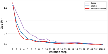
Figure 4. Comparison of the performance of DEITSP with three types of noise schedules and various iteration steps.

Comparison of the performance of DEITSP with three types of noise schedules and various iteration steps.

4.5. Ablation Studies

In this subsection, we conduct a series of ablation experiments to evaluate the effectiveness of our proposed graph transformer and iteration strategy on 50-node test instances. We systematically modify key components to assess their impact. First, we analyze the effects of different noise schedules and iteration steps on performance, as shown in Figure 4. Second, we examine the impact of key components using Table 4. In the W/o DML (Dual-Modal Learning) variant, we substitute our proposed graph transformer with the anisotropic graph neural network introduced in (Sun and Yang, 2023). In the W/o EI (Efficient Iteration) variant, we replace our unique iteration strategy with the standard DDIM paradigm employed in (Sun and Yang, 2023; Ma and Dou, 2024; Li et al., 2024). Figure 4 illustrates that our inverse function noise schedule generally outperforms other schedules across various iteration steps. Table 4, which compares these modifications, shows that our graph transformer network consistently achieves superior results in both average solution length and inference time, with the performance gap widening as the number of iteration steps increases. Additionally, the table indicates that our iteration process significantly surpasses the standard DDIM paradigm. Notably, our 1-step results outperform DDIM’s 10-step results, and our 5-step results exceed DDIM’s 50-step results, highlighting the efficiency and effectiveness of our approach.

Table 4. Ablation studies on our proposed components

Iteration Step		1	5	10	15	20	30	40	50
W/o DML	Gap(%)	0.24	0.09	0.07	0.07	0.05	0.06	0.05	0.05
	Time(s)	20.00	56.20	107.67	158.15	212.88	319.88	425.89	529.35
W/o EI	Gap(%)	1.68	0.23	0.11	0.10	0.09	0.10	0.11	0.11
	Time(s)	13.64	32.88	62.99	119.25	123.83	184.33	253.63	305.93
DEITSP	Gap(%)	0.13	0.03	0.02	0.01	0.01	0.01	0.01	0.00
	Time(s)	14.95	37.85	72.00	127.62	146.09	218.14	297.14	369.81

5. Conclusion

In this paper, we introduced a diffusion-based non-autoregressive model named DEITSP, which is specifically designed for solving the Traveling Salesman Problem (TSP). We proposed a dual-modality graph transformer and an efficient iterative strategy, achieving superior solution quality and inference speed compared to state-of-the-art methods. DEITSP’s flexibility in adjusting iteration steps allows it to balance computation time with solution accuracy, and its strong generalization capability is evident across diverse real-world instances and benchmarks in our experiments.

While current diffusion-based approaches demonstrate strong performance, training with labeled data can present challenges when scaling to extremely large instances. We recognize this as an area for further improvement and will explore more efficient methods to enhance scalability, such as decomposing problems into smaller sub-problems (Fu et al., 2021) or designing new unsupervised training mechanisms. Additionally, future work will focus on extending DEITSP to address a broader range of optimization problems, incorporating more complex constraints and varied environments, and further enhancing its robustness and applicability.

Appendix A Decoding Strategy

The diffusion model generates an adjacency matrix heatmap score that represents the connection probability of each edge. However, these adjacency matrices cannot ensure the feasibility of meeting TSP constraints. Therefore, a specialized decoding strategy is required to produce feasible solutions. We employ a combination of Greedy decoding and 2-opt as the default strategy for our experiments, following Sun and Yang (2023); Graikos et al. (2022). In the greedy decoding method, we sort the edges based on $(\tilde{a}_{ij}+\tilde{a}_{ji})/cost(v_{i},v_{j})$, and degressively insert them into the partial solution while ensuring no conflict.

Appendix B Noise Schedule

As depicted in Figures 9, 10, and 11, the sparsity of TSP solutions leads to a significant difference in distribution between the optimal solution and the high-noise state. While higher noise levels expand the exploration range, they also increase inaccuracies in network predictions. Therefore, our proposed schedule, unlike the conventional linear and cosine schedules used in image generation, prioritizes more iterations in a low-noise state. To illustrate, Figure 5 presents the time step values for different schedules, using 10 steps as an example.

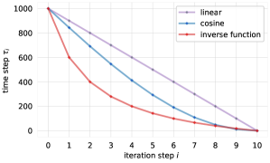
Figure 5. Comparison of noise step values with different iteration schedules (linear, cosine, and inverse function).

Comparison of noise step values with different iteration schedules

Appendix C Generalization to Real-World Instances

Unlike the uniformly sampled node coordinates used in training, the node coordinates in real-world TSPLIB instances are derived from authentic or carefully designed scenarios, reflecting structural and contextual similarities to real-world challenges. We apply models trained on TSP100 instances directly to 26 real-world instances, a strategy known as zero-shot generalization (Joshi et al., 2022). The ability of a model to generate satisfactory solutions under these conditions highlights its proficiency in recognizing and learning the fundamental patterns of TSPs, making it suitable for a wide range of applications beyond mere pattern recognition. Tables 5 and Table 6 show the performance of neural network-based approaches on 26 TSPLIB instances.

Appendix D Visualization of the Noise Addition Process

We visualize the noise addition process in DEITSP, which disrupts the optimal TSP solution. We utilize instances of TSP20 (TSP with 20 nodes), TSP50, and TSP100, and set them according to the Eq. (2), where $t$ is the parameter representing the noise level. We visualize the noisy instances in the form of graphs and adjacency matrices. As shown in the Figure 9 and Figure 10, with the increase of noise level, the adjacency matrix of TSP instances gradually transforms into a uniformly distributed pattern.

Appendix E Visualization of the Inference Process

To visually illustrate the iterative exploration of multiple solutions during the DEITSP inference process, we present visualizations of the process. We utilize randomly generated instances of TSP20, TSP50 and TSP100, adhering to the same experimental settings outlined in Section 4.1. These visualizations encompass the initial solution derived from uniform sampling, the solution predicted by the diffusion model, and the ground truth, all presented in the form of graphs and adjacency matrices. As evident from Figures 6, 7 and 8, DEITSP demonstrates its ability to predict high-quality solutions through a single-step denoising process and further enhances its performance by exploring a broader range of solutions over iterations. Notably, as the number of iteration steps increases, the quality of the predicted solutions gradually improves, thereby validating the efficacy of our noise scheduling strategy in optimizing the solution space.

Figure 6. Visualization of solutions produced by DEITSP using 4 iteration steps on TSP20 instances.

Visualization of solutions produced by DEITSP using 4 step iterations.

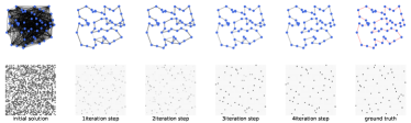
Figure 7. Visualization of solutions produced by DEITSP using 4 iteration steps on TSP50 instances.

Visualization of solutions produced by DEITSP using 4 step iterations.

Figure 8. Visualization of solutions produced by DEITSP using 4 iteration steps on TSP100 instances.

Visualization of solutions produced by DEITSP using 4 step iterations.

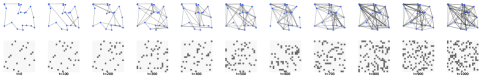
Figure 9. Visualization of noise addition process on the TSP20 instance.

Visualization of solutions produced by DEITSP using 4 step iterations.

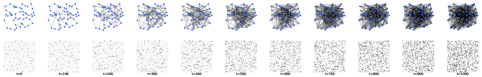
Figure 10. Visualization of noise addition process on the TSP50 instance.

Visualization of solutions produced by DEITSP using 4 step iterations.

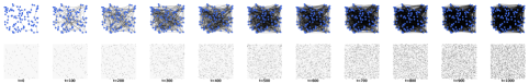
Figure 11. Visualization of noise addition process on the TSP100 instance.

Visualization of solutions produced by DEITSP using 4 step iterations.

Table 5. Generalization performance of applying models trained using TSP100 instances on TSPLIB instances (Part 1)

Name	Optimal Len	AM			POMO			Sym-NCO			ELG			HierTSP
		Len	Gap (%)	Time (s)	Len	Gap (%)	Time (s)	Len	Gap (%)	Time (s)	Len	Gap (%)	Time (s)	Len	Gap (%)	Time (s)
berlin52	7542.000	7856.426	4.169	0.129	7544.366	0.031	0.837	7544.662	0.035	0.851	7544.365	0.031	0.917	7544.662	0.035	0.872
bier127	118282.000	125270.101	5.908	0.522	123319.180	4.259	0.086	123993.359	4.829	0.092	122855.531	3.867	0.244	124093.656	4.913	0.125
ch130	6110.000	6304.420	3.182	0.550	6122.857	0.210	0.088	6118.715	0.143	0.090	6119.898	0.162	0.247	6157.908	0.784	0.131
ch150	6528.000	6827.244	4.584	0.697	6562.099	0.522	0.102	6567.454	0.604	0.104	6583.826	0.855	0.288	6578.063	0.767	0.147
eil101	629.000	647.832	2.994	0.359	640.596	1.844	0.070	640.212	1.782	0.071	643.840	2.359	0.193	642.830	2.199	0.100
eil51	426.000	432.935	1.628	0.125	431.953	1.397	0.037	431.953	1.397	0.038	430.746	1.114	0.098	429.484	0.818	0.054
eil76	538.000	548.717	1.992	0.225	544.369	1.184	0.053	544.652	1.236	0.055	549.433	2.125	0.146	547.020	1.677	0.078
kroA100	21282.000	22136.898	4.017	0.352	21396.438	0.538	0.071	21357.164	0.353	0.073	21307.422	0.119	0.192	21487.941	0.968	0.102
kroA150	26524.000	27527.668	3.784	0.695	26734.875	0.795	0.100	26890.738	1.383	0.103	26805.207	1.060	0.286	26995.578	1.778	0.146
kroA200	29368.000	31454.890	7.106	1.150	29984.789	2.100	0.134	30206.396	2.855	0.137	29831.221	1.577	0.383	30149.805	2.662	0.188
kroB100	22141.000	23279.490	5.142	0.352	22275.605	0.608	0.068	22374.285	1.054	0.070	22280.641	0.631	0.191	22275.350	0.607	0.099
kroB150	26130.000	26766.788	2.437	0.696	26635.195	1.933	0.100	26816.086	2.626	0.103	26374.766	0.937	0.288	26638.965	1.948	0.148
kroB200	29437.000	31951.214	8.541	1.150	30428.590	3.369	0.136	30563.463	3.827	0.140	29904.586	1.588	0.385	30551.854	3.787	0.188
kroC100	20749.000	20950.680	0.972	0.352	20832.773	0.404	0.068	20959.719	1.016	0.070	20770.041	0.101	0.194	20829.061	0.386	0.099
kroD100	21294.000	21872.558	2.717	0.352	21719.195	1.997	0.068	21635.557	1.604	0.070	21532.164	1.118	0.191	21772.988	2.249	0.102
kroE100	22068.000	22392.400	1.470	0.352	22380.355	1.415	0.068	22346.006	1.260	0.070	22237.137	0.766	0.194	22260.621	0.873	0.100
lin105	14379.000	14629.051	1.739	0.380	14494.633	0.804	0.072	14648.303	1.873	0.074	14467.038	0.612	0.200	14720.170	2.373	0.103
pr107	44303.000	46045.437	3.933	0.391	44897.246	1.341	0.073	45324.367	2.305	0.075	44960.422	1.484	0.205	44958.227	1.479	0.106
pr124	59030.000	61200.533	3.677	0.499	59091.836	0.105	0.083	59123.277	0.158	0.086	59181.652	0.257	0.236	59520.555	0.831	0.121
pr136	96772.000	101672.534	5.064	0.585	97485.609	0.737	0.095	97513.648	0.766	0.097	97733.406	0.993	0.259	98391.383	1.673	0.136
pr144	58537.000	63009.812	7.641	0.638	58828.539	0.498	0.097	59043.488	0.865	0.099	58859.398	0.551	0.275	58795.152	0.441	0.140
pr152	73682.000	79203.729	7.494	0.708	74440.711	1.030	0.102	76061.063	3.229	0.104	73720.609	0.052	0.292	74485.031	1.090	0.147
pr76	108159.000	109041.577	0.816	0.226	108159.438	0.000	0.053	108591.000	0.399	0.054	108444.047	0.264	0.145	108428.906	0.250	0.077
rat195	2323.000	2483.124	6.893	1.114	2558.470	10.136	0.130	2569.150	10.596	0.132	2400.775	3.348	0.372	2492.917	7.315	0.186
rat99	1211.000	1243.031	2.645	0.347	1273.635	5.172	0.068	1264.701	4.434	0.072	1248.142	3.067	0.189	1240.427	2.430	0.098
st70	675.000	686.725	1.737	0.200	677.110	0.313	0.052	677.110	0.313	0.051	677.110	0.313	0.134	677.110	0.313	0.071
Mean	31466.115	32703.968	3.934	0.506	31902.325	1.644	0.112	32069.482	1.959	0.115	31825.516	1.129	0.259	32025.602	1.717	0.149
”Gap” indicate length differences compared to the optimal solutions from TSPLIB.

Table 6. Generalization performance of applying models trained using TSP100 instances on TSPLIB instances (Part 2)

Name	Optimal Len	DIFUSCO			T2TCO			DEITSP(1 Iter)			DEITSP(4 Iter)			DEITSP(16 Iter)
		Len	Gap (%)	Time (s)	Len	Gap (%)	Time (s)	Len	Gap (%)	Time (s)	Len	Gap (%)	Time (s)	Len	Gap	Time
berlin52	7542.000	7544.366	0.031	0.447	7544.366	0.031	0.749	7544.366	0.031	0.017	7544.366	0.031	0.047	7544.366	0.031	0.119
bier127	118282.000	119512.524	1.040	0.638	119050.160	0.649	0.953	119951.880	1.412	0.039	118885.507	0.510	0.096	119367.517	0.918	0.236
ch130	6110.000	6190.983	1.325	0.700	6122.493	0.204	1.035	6152.278	0.692	0.048	6152.278	0.692	0.113	6126.887	0.276	0.237
ch150	6528.000	6585.461	0.880	0.867	6580.991	0.812	1.295	6590.877	0.963	0.045	6580.099	0.798	0.106	6564.298	0.556	0.286
eil101	629.000	641.458	1.981	0.473	642.556	2.155	0.797	652.587	3.750	0.028	644.122	2.404	0.058	644.122	2.404	0.159
eil51	426.000	431.271	1.237	3.061	429.484	0.818	2.413	433.943	1.865	2.646	429.484	0.818	2.678	433.443	1.747	2.653
eil76	538.000	545.048	1.310	0.469	556.769	3.489	0.769	544.369	1.184	0.019	544.369	1.184	0.046	544.369	1.184	0.134
kroA100	21282.000	21285.443	0.016	0.483	21285.443	0.016	0.763	21307.422	0.119	0.031	21307.422	0.119	0.058	21307.422	0.119	0.159
kroA150	26524.000	26578.099	0.204	0.845	26525.031	0.004	1.251	27048.654	1.978	0.048	26900.181	1.418	0.103	26804.307	1.057	0.285
kroA200	29368.000	29583.978	0.735	1.414	30033.710	2.267	2.103	29718.696	1.194	0.072	29666.192	1.015	0.147	29543.848	0.599	0.490
kroB100	22141.000	22533.086	1.771	0.510	22645.401	2.278	0.772	22257.483	0.526	0.026	22303.429	0.734	0.055	22268.685	0.577	0.187
kroB150	26130.000	26284.696	0.592	0.850	26244.185	0.437	1.249	26547.005	1.596	0.046	26410.273	1.073	0.105	26319.820	0.726	0.289
kroB200	29437.000	30204.181	2.606	1.474	29841.325	1.374	2.102	30841.207	4.770	0.072	29898.069	1.566	0.171	29639.831	0.689	0.472
kroC100	20749.000	20773.073	0.116	0.492	20750.763	0.008	0.755	21299.404	2.653	0.027	20943.158	0.936	0.056	21293.943	2.626	0.170
kroD100	21294.000	21320.974	0.127	0.504	21294.291	0.001	0.778	21460.117	0.780	0.027	21460.117	0.780	0.064	21375.452	0.383	0.205
kroE100	22068.000	22372.583	1.380	0.498	22362.472	1.334	0.769	22806.209	3.345	0.024	22444.825	1.708	0.059	22427.985	1.631	0.168
lin105	14379.000	14432.139	0.370	0.524	14382.996	0.028	0.802	14382.996	0.028	0.037	14439.703	0.422	0.086	14382.996	0.028	0.183
pr107	44303.000	45551.263	2.818	0.531	44590.338	0.649	0.806	44897.401	1.342	0.032	44382.709	0.180	0.089	44519.916	0.490	0.179
pr124	59030.000	59814.535	1.329	0.602	59774.850	1.262	0.903	59632.923	1.021	0.032	59396.847	0.621	0.074	59607.740	0.979	0.234
pr136	96772.000	97664.229	0.922	0.711	96925.555	0.159	1.072	100361.346	3.709	0.048	98778.220	2.073	0.114	98097.238	1.369	0.252
pr144	58537.000	58853.339	0.540	0.767	59287.317	1.282	1.146	58620.693	0.143	0.059	58620.693	0.143	0.097	58604.905	0.116	0.272
pr152	73682.000	75613.977	2.622	0.865	74610.427	1.260	1.282	74448.987	1.041	0.068	75151.014	1.994	0.106	73683.641	0.002	0.292
pr76	108159.000	110019.494	1.720	0.439	109770.304	1.490	0.756	110247.698	1.931	0.016	109086.647	0.858	0.063	109160.652	0.926	0.131
rat195	2323.000	2392.573	2.995	1.371	2365.187	1.816	2.079	2366.034	1.853	0.058	2355.270	1.389	0.143	2350.777	1.196	0.452
rat99	1211.000	1220.098	0.751	0.562	1219.244	0.681	0.804	1221.318	0.852	0.033	1221.318	0.852	0.052	1219.244	0.681	0.153
st70	675.000	677.642	0.391	0.459	677.194	0.325	0.758	677.194	0.325	0.017	677.194	0.325	0.039	677.110	0.313	0.121
Mean	31466.115	31870.251	1.147	0.791	31750.494	0.955	1.114	32000.503	1.504	0.139	31777.827	0.948	0.185	31711.943	0.832	0.328
”Gap” indicate length differences compared to the optimal solutions from TSPLIB.

References

- (1)
- Applegate et al. (2007) David L. Applegate, Robert E. Bixby, Vašek Chvátal, and William John Cook. 2007. The Traveling Salesman Problem: A Computational Study. Princeton University Press.
- Austin et al. (2021) Jacob Austin, Daniel D Johnson, Jonathan Ho, Daniel Tarlow, and Rianne Van Den Berg. 2021. Structured denoising diffusion models in discrete state-spaces. Advances in Neural Information Processing Systems 34 (2021), 17981–17993.
- Bahdanau et al. (2015) Dzmitry Bahdanau, Kyunghyun Cho, and Yoshua Bengio. 2015. Neural machine translation by jointly learning to align and translate. In Proceedings of International Conference on Learning Representations.
- Bansal et al. (2004) Nikhil Bansal, Avrim Blum, Shuchi Chawla, and Adam Meyerson. 2004. Approximation Algorithms for Deadline-TSP and Vehicle Routing with Time-Windows. In Proceedings of the Annual ACM Symposium on Theory of Computing. 166–174.
- Bellman (1962) Richard Bellman. 1962. Dynamic programming treatment of the travelling salesman problem. J. ACM 9, 1 (1962), 61–63.
- Bello et al. (2017) Irwan Bello, Hieu Pham, Quoc Viet Le, Mohammad Norouzi, and Samy Bengio. 2017. Neural combinatorial optimization with reinforcement learning. In Proceedings of International Conference on Learning Representations Workshop.
- Bresson and Laurent (2021) Xavier Bresson and Thomas Laurent. 2021. The transformer network for the traveling salesman problem. arXiv:2103.03012
- Chen et al. (2023) Ting Chen, Ruixiang Zhang, and Geoffrey Hinton. 2023. Analog Bits: Generating Discrete Data using Diffusion Models with Self-Conditioning. In The Eleventh International Conference on Learning Representations. https://openreview.net/forum?id=3itjR9QxFw
- Christiansen et al. (2004) Marielle Christiansen, Kjetil Fagerholt, and David Ronen. 2004. Ship routing and scheduling: status and perspectives. Transportation Science 38 (2004), 1–18.
- Deudon et al. (2018) Michel Deudon, Pierre Cournut, Alexandre Lacoste, Yossiri Adulyasak, and Louis-Martin Rousseau. 2018. Learning heuristics for the TSP by policy gradient. In Proceedings of Integration of Constraint Programming, Artificial Intelligence, and Operations Research. 170–181.
- Fu et al. (2021) Zhanghua Fu, Kaibin Qiu, and Hongyuan Zha. 2021. Generalize a small pre-trained model to arbitrarily large TSP instances. In Proceedings of the AAAI Conference on Artificial Intelligence. 7474–7482.
- Gao et al. (2023) Chengrui Gao, Haopu Shang, Ke Xue, Dong Li, and Chao Qian. 2023. Towards generalizable neural solvers for vehicle routing problems via ensemble with transferrable local policy. arXiv preprint arXiv:2308.14104 (2023).
- Garey and Johnson (1990) Michael Randolph Garey and David Stifler Johnson. 1990. Computers and Intractability; A Guide to the Theory of NP-Completeness. W. H. Freeman & Co.
- Goh et al. (2024) Yong Liang Goh, Zhiguang Cao, Yining Ma, Yanfei Dong, Mohammed Haroon Dupty, and Wee Sun Lee. 2024. Hierarchical Neural Constructive Solver for Real-world TSP Scenarios. In Proceedings of the 30th ACM SIGKDD Conference on Knowledge Discovery and Data Mining. 2120–2131.
- Graikos et al. (2022) Alexandros Graikos, Nikolay Malkin, Nebojsa Jojic, and Dimitris Samaras. 2022. Diffusion models as plug-and-play priors. Advances in Neural Information Processing Systems 35 (2022), 14715–14728.
- Helsgaun (2017) Keld Helsgaun. 2017. An extension of the Lin–Kernighan–Helsgaun TSP solver for constrained traveling salesman and vehicle routing problems. Roskilde: Roskilde University (2017), 24–50.
- Ho et al. (2020) Jonathan Ho, Ajay Jain, and Pieter Abbeel. 2020. Denoising diffusion probabilistic models. Advances in neural information processing systems 33 (2020), 6840–6851.
- Hussain et al. (2022) Md Shamim Hussain, Mohammed J Zaki, and Dharmashankar Subramanian. 2022. Global Self-Attention as a Replacement for Graph Convolution. In ACM SIGKDD International Conference on Knowledge Discovery and Data Mining.
- Jiang et al. (2023b) Yuan Jiang, Zhiguang Cao, Yaoxin Wu, Wen Song, and Jie Zhang. 2023b. Ensemble-based deep reinforcement learning for vehicle routing problems under distribution shift. Advances in Neural Information Processing Systems 36 (2023).
- Jiang et al. (2023a) Yuan Jiang, Zhiguang Cao, Yaoxin Wu, and Jie Zhang. 2023a. Multi-view graph contrastive learning for solving vehicle routing problems. In Proceedings of the Thirty-Ninth Conference on Uncertainty in Artificial Intelligence (Proceedings of Machine Learning Research, Vol. 216), Robin J. Evans and Ilya Shpitser (Eds.). PMLR, 984–994. https://proceedings.mlr.press/v216/jiang23a.html
- Jin et al. (2023) Yan Jin, Yuandong Ding, Xuanhao Pan, Kun He, Li Zhao, Tao Qin, Lei Song, and Jiang Bian. 2023. Pointerformer: Deep reinforced multi-pointer transformer for the traveling salesman problem. In Proceedings of the AAAI Conference on Artificial Intelligence, Vol. 37. 8132–8140.
- Joshi et al. (2022) Chaitanya K. Joshi, Quentin Cappart, Louis-Martin Rousseau, and Thomas Laurent. 2022. Learning the travelling salesperson problem requires rethinking generalization. Constraints 27 (2022), 70–98.
- Joshi et al. (2019) Chaitanya K. Joshi, Thomas Laurent, and Xavier Bresson. 2019. An efficient graph convolutional network technique for the travelling salesman problem. In Proceedings of INFORMS Annual Meeting, Session on Boosting Combinatorial Optimization using Machine Learning. 1–17.
- Jung et al. (2023) Minseop Jung, Jaeseung Lee, and Jibum Kim. 2023. A Lightweight CNN-Transformer Model for Learning Traveling Salesman Problems. arXiv preprint arXiv:2305.01883 (2023).
- Kim et al. (2021) Minsu Kim, Jinkyoo Park, and Joungho Kim. 2021. Learning Collaborative Policies to Solve NP-hard Routing Problems. In Proceedings of Advances in Neural Information Processing Systems, Vol. 34. 10418–10430.
- Kim et al. (2022) Minsu Kim, Junyoung Park, and Jinkyoo Park. 2022. Sym-NCO: Leveraging Symmetricity for Neural Combinatorial Optimization. In Proceedings of Advances in Neural Information Processing Systems, Vol. 35. 1936–1949.
- Kizilateş and Nuriyeva (2013) Gözde Kizilateş and Fidan Nuriyeva. 2013. On the nearest neighbor algorithms for the traveling salesman problem. In Advances in Computational Science, Engineering and Information Technology: Proceedings of the Third International Conference on Computational Science, Engineering and Information Technology (CCSEIT-2013), KTO Karatay University, June 7-9, 2013, Konya, Turkey-Volume 1. Springer, 111–118.
- Kool et al. (2019) Wouter Kool, Herke van Hoof, and Max Welling. 2019. Attention, Learn to solve routing problems!. In Proceedings of International Conference on Learning Representations.
- Kwon et al. (2020) Yeong-Dae Kwon, Jinho Choo, Byoungjip Kim, Iljoo Yoon, Youngjune Gwon, and Seungjai Min. 2020. POMO: Policy Optimization with Multiple Optima for Reinforcement Learning. In Proceedings of Advances in Neural Information Processing Systems. 21188–21198.
- Li et al. (2021) Kaiwen Li, Tao Zhang, Rui Wang, Wenjian Qin, Hui-hui He, and Hong Huang. 2021. Research reviews of combinatorial optimization methods based on deep reinforcement learning. Zidonghua Xuebao/Acta Automatica Sinica 47 (2021), 2521–2537.
- Li et al. (2024) Yang Li, Jinpei Guo, Runzhong Wang, and Junchi Yan. 2024. From distribution learning in training to gradient search in testing for combinatorial optimization. Advances in Neural Information Processing Systems 36 (2024).
- Lin and Kernighan (1973) Shen Lin and Brian W Kernighan. 1973. An effective heuristic algorithm for the traveling-salesman problem. Operations research 21, 2 (1973), 498–516.
- Luo et al. (2023) Simian Luo, Yiqin Tan, Longbo Huang, Jian Li, and Hang Zhao. 2023. Latent consistency models: Synthesizing high-resolution images with few-step inference. arXiv preprint arXiv:2310.04378 (2023).
- Ma and Dou (2024) Ning Ma and Yishun Dou. 2024. Semi-supervised Diffusion Solver for Travelling Salesman Problem. https://openreview.net/forum?id=0u9uvPdRgV
- Ma et al. (2021) Yining Ma, Jingwen Li, Zhiguang Cao, Wen Song, Le Zhang, Zhenghua Chen, and Jing Tang. 2021. Learning to Iteratively Solve Routing Problems with Dual-Aspect Collaborative Transformer. In Proceedings of Advances in Neural Information Processing Systems, Vol. 34. 11096–11107.
- Nazari et al. (2018) Mohammadreza Nazari, Afshin Oroojlooy, Martin Takáč, and Lawrence V. Snyder. 2018. Reinforcement Learning for Solving the Vehicle Routing Problem. In Proceedings of Advances in Neural Information Processing Systems. 9861––9871.
- Nowak et al. (2018) Alex Nowak, David Folqué, and Joan Bruna. 2018. Divide and conquer Networks. In Proceedings of International Conference on Learning Representations.
- Onizawa et al. (2022) Naoya Onizawa, Kota Katsuki, Duckgyu Shin, Warren J Gross, and Takahiro Hanyu. 2022. Fast-converging simulated annealing for Ising models based on integral stochastic computing. IEEE Transactions on Neural Networks and Learning Systems 34, 12 (2022), 10999–11005.
- Padberg and Rinaldi (1991) Manfred Padberg and Giovanni Rinaldi. 1991. A branch-and-cut algorithm for the resolution of large-scale symmetric traveling salesman problems. SIAM Rev. 33 (1991), 60–100.
- Ran et al. (2021) Qiu Ran, Yankai Lin, Peng Li, and Jie Zhou. 2021. Guiding non-autoregressive neural machine translation decoding with reordering information. In Proceedings of the AAAI Conference on Artificial Intelligence. 13727–13735.
- Reinelt (1991) Gerhard Reinelt. 1991. TSPLIB—A traveling salesman problem library. ORSA journal on computing 3, 4 (1991), 376–384. https://www.math.uwaterloo.ca/tsp/index.html
- Song et al. (2020) Jiaming Song, Chenlin Meng, and Stefano Ermon. 2020. Denoising Diffusion Implicit Models. arXiv:2010.02502 (October 2020). https://arxiv.org/abs/2010.02502
- Song et al. (2023) Yang Song, Prafulla Dhariwal, Mark Chen, and Ilya Sutskever. 2023. Consistency Models. arXiv preprint arXiv:2303.01469 (2023).
- Sun and Yang (2023) Zhiqing Sun and Yiming Yang. 2023. DIFUSCO: Graph-based Diffusion Solvers for Combinatorial Optimization. In Proceedings of Advances in Neural Information Processing Systems.
- Vaswani et al. (2017) Ashish Vaswani, Noam Shazeer, Niki Parmar, Jakob Uszkoreit, Llion Jones, Aidan N Gomez, Łukasz Kaiser, and Illia Polosukhin. 2017. Attention is all you Need. In Proceedings of Advances in Neural Information Processing Systems. 6000––6010.
- Vignac et al. (2023) Clement Vignac, Igor Krawczuk, Antoine Siraudin, Bohan Wang, Volkan Cevher, and Pascal Frossard. 2023. DiGress: Discrete Denoising diffusion for graph generation. In The Eleventh International Conference on Learning Representations. https://openreview.net/forum?id=UaAD-Nu86WX
- Vinyals et al. (2015) Oriol Vinyals, Meire Fortunato, and Navdeep Jaitly. 2015. Pointer networks. In Proceedings of Advances in Neural Information Processing Systems. 2692––2700.
- Wang et al. (2019) Lei Wang, Yubin Xiao, Jiechen Li, Xiang Feng, Qian Li, and Jialiang Yang. 2019. IIRWR: Internal inclined random walk with restart for lncRNA-Disease association prediction. IEEE Access 7 (2019), 54034–54041.
- Wu et al. (2023a) Xuan Wu, Jizong Han, Di Wang, Pengyue Gao, Quanlong Cui, Liang Chen, Yanchun Liang, Han Huang, Heow Pueh Lee, Chunyan Miao, You Zhou, and Chunguo Wu. 2023a. Incorporating Surprisingly Popular Algorithm and Euclidean distance-based adaptive topology into PSO. Swarm and Evolutionary Computation 76 (2023), 101222.
- Wu et al. (2023b) Xuan Wu, Di Wang, Huanhuan Chen, Lele Yan, Yubin Xiao, Chunyan Miao, Hongwei Ge, Dong Xu, Yanchun Liang, Kangping Wang, et al. 2023b. Neural Architecture Search for Text Classification With Limited Computing Resources Using Efficient Cartesian Genetic Programming. IEEE Transactions on Evolutionary Computation (2023).
- Wu et al. (2024) Xuan Wu, Di Wang, Lijie Wen, Yubin Xiao, Chunguo Wu, Yuesong Wu, Chaoyu Yu, Douglas L. Maskell, and You Zhou. 2024. Neural Combinatorial Optimization Algorithms for Solving Vehicle Routing Problems: A Comprehensive Survey with Perspectives. arXiv:2406.00415 [cs.AI]
- Xiao et al. (2023) Yubin Xiao, Di Wang, Huanhuan Chen, Boyang Li, Wei Pang, Xuan Wu, Hao Li, Dong Xu, Yanchun Liang, and You Zhou. 2023. Reinforcement learning-based non-autoregressive solver for traveling salesman problems. arXiv preprint arXiv:2308.00560 (2023).
- Xiao et al. (2024a) Yubin Xiao, Di Wang, Boyang Li, Mingzhao Wang, Xuan Wu, Changliang Zhou, and You Zhou. 2024a. Distilling autoregressive models to obtain high-performance non-autoregressive solvers for vehicle routing problems with faster inference speed. In Proceedings of the AAAI Conference on Artificial Intelligence, Vol. 38. 20274–20283.
- Xiao et al. (2024b) Yubin Xiao, Di Wang, Xuan Wu, Yuesong Wu, Boyang Li, Wei Du, Liupu Wang, and You Zhou. 2024b. Improving Generalization of Neural Vehicle Routing Problem Solvers Through the Lens of Model Architecture. arXiv preprint arXiv:2406.06652 (2024).
- Xiao et al. (2020) Yubin Xiao, Zheng Xiao, Xiang Feng, Zhiping Chen, Linai Kuang, and Lei Wang. 2020. A novel computational model for predicting potential LncRNA-disease associations based on both direct and indirect features of LncRNA-disease pairs. BMC Bioinformatics 21 (2020), 1–22.
- Xin et al. (2021) Liang Xin, Wen Song, Zhiguang Cao, and Jie Zhang. 2021. Multi-Decoder Attention Model with Embedding Glimpse for Solving Vehicle Routing Problems. In Proceeding of the AAAI Conference on Artificial Intelligence. 12042–12049.
- Xu et al. (2018) Zhe Xu, Zhixin Li, Qingwen Guan, Dingshui Zhang, Qiang Li, Junxiao Nan, Chunyang Liu, Wei Bian, and Jieping Ye. 2018. Large-scale order dispatch in on-demand ride-hailing platforms: A learning and planning approach. In Proceedings of the 24th ACM SIGKDD international conference on knowledge discovery & data mining. 905–913.
- Zhong et al. (2018) Yiwen Zhong, Juan Lin, Lijin Wang, and Hui Zhang. 2018. Discrete comprehensive learning particle swarm optimization algorithm with Metropolis acceptance criterion for traveling salesman problem. Swarm and Evolutionary Computation 42 (2018), 77–88.