Optical Images of Mini Boson Stars in Palatini $f(R)$ Gravity

Abstract

We investigate the optical properties of mini boson stars within the framework of Palatini $f(R)$ gravity, adopting a quadratic form $f(R)=R+\xi R^{2}$, where $\xi$ is the gravitational coupling constant. By deriving the modified scalar Lagrangian and solving the field equations numerically, we explore photon trajectories and the resulting optical images under spherical light sources and thin accretion disks. Unlike Schwarzschild black holes (BHs), boson stars lack stable photon rings due to the positive second derivative of their effective potential. Consequently, their images are dominated by direct emissions from photons completing a single orbit. The study examines the dependence of the optical characteristics on the initial scalar field $\psi_{0}$ and the coupling parameter $\xi$. Numerical results include effective potentials, redshift maps, and detailed imaging of boson stars, providing insights into distinguishing boson stars from black holes using high-resolution astronomical observations.

1 Introduction

In recent years, gravitational wave detections by LIGO and Virgo have provided unprecedented insights into the universe, enabling detailed investigations of massive compact objects and advancing our understanding of binary black holes (BBH) formation mechanisms [1, 2]. These observations have not only constrained the mass spectrum of BBH systems, bridging the gap between the heaviest neutron stars and stellar-mass BHs (e.g., the GW190814 event [3]), but also highlighted significant discrepancies with predictions from current stellar evolution models [4]. Resolving these tensions between theoretical frameworks and observational evidence has emerged as a critical challenge in contemporary astrophysical research.

Compact objects with masses in the range of 50–100 $M_{\odot}$ have posed significant challenges to our understanding of intermediate-mass BH mergers [5, 6, 7]. While Kerr BHs have traditionally been considered the primary progenitors of such merger events, the formation pathways leading to BHs of these observed masses remain largely unresolved. Moreover, recent observations suggest that the mergers of other massive, non-luminous compact objects could potentially account for these phenomena [6, 7]. These alternative candidates, often referred to as ”exotic compact objects” (ECOs) [8], have gained additional attention due to corroborative evidence from electromagnetic spectrum observations [9].

Among ECOs, boson stars occupy a prominent position due to their unique theoretical properties. These ultracompact objects, composed of bosons bound by self-gravity, exhibit a wide range of masses and sizes—from atomic scales to astrophysical dimensions—depending on the boson mass. Since the foundational studies by Kaup [10], Ruffini and Bonnazola [11], boson stars have been the subject of extensive research, focusing on their stability and dynamical properties [12, 13].

Numerical simulations have demonstrated that both rotating and non-rotating boson stars can achieve masses on the order of several solar masses $M_{\odot}$, consistent with astrophysical observations, while lacking an event horizon. Under the assumption of spherical symmetry, boson stars are capable of forming binary systems, and the resulting gravitational wave emissions can be directly compared with those from BBH mergers [14, 15]. Beyond spherically symmetric configurations, axisymmetric rotating boson star equilibrium sequences have been successfully constructed [16, 17, 18], and the dynamics of merging binary rotating boson stars have been explored through simulations [19, 20].

In the realm of supermassive compact objects, boson stars have been proposed as potential alternatives to BHs, with some studies suggesting that the Galactic Center object, Sgr A*, could be a boson star [21]. Under the thin-disk approximation, Rosa investigated optical images of boson stars, excluding gravitational coupling effects [22, 23]. Furthermore, boson stars have been proposed as replacements for BHs as the central objects in accretion systems [24]. While the optical images of boson stars and BHs share similarities, current observational techniques, under specific assumptions, provide sufficient resolution to distinguish between the two types of objects [25].

The shadow images of black holes in different accretion disk models have been extensively studied [26, 27, 28, 29, 30, 31, 32, 33, 34, 35, 36]. Therefore, this paper will focus on the optical images of boson stars. To further investigate their physical properties and optical images, we introduce the Palatini $f(R)$ gravity theory [37, 38]. This is a modified framework of general relativity, which alters the dynamics of the gravitational field by introducing a function $f(R)$ that depends on the scalar curvature $R$. Unlike the traditional $f(R)$ theories, the Palatini approach assumes that the metric and the affine connection are independent [39], enabling the incorporation of nonlinear correction terms within the framework of general relativity. This approach provides a promising avenue for alternative theories of gravity, offering an explanation for large-scale cosmological phenomena without invoking dark matter or dark energy. Additionally, it establishes a theoretical basis for addressing singularity problems and introducing modifications at high energy scales.

To further explore the physical properties and optical signatures of boson stars, we adopt the Palatini $f(R)$ gravity theory [37, 38]. This framework modifies general relativity by introducing a function $f(R)$ that depends on the scalar curvature $R$, altering the gravitational field dynamics. Unlike traditional $f(R)$ theories, the Palatini formulation treats the metric and affine connection as independent variables [39], thereby allowing for the inclusion of nonlinear correction terms within the general relativistic paradigm. The Palatini approach offers a robust framework for alternative theories of gravity, providing insights into large-scale cosmological phenomena without relying on dark matter or dark energy. Furthermore, it offers a potential resolution to singularity issues and introduces modifications relevant at high energy scales, making it a compelling candidate for investigating the theoretical foundations and observational implications of boson stars.

The absence of an event horizon in ECOs allows for direct observation of their innermost regions, presenting a unique opportunity to extend and test general relativity in novel regimes. This makes the investigation of how modified Lagrangian terms influence the physical properties of boson stars, such as mass and radius, an important area of research [40]. Given the flexibility of the Palatini $f(R)$ gravity theory and its simplicity in field equations, this study focuses on analyzing its impact on the optical images of boson stars. Furthermore, extensive research has explored boson stars within other modified gravitational frameworks, including scalar-tensor theories [41], Horndeski theory [42], and models incorporating Gauss-Bonnet coupling [43]. These studies provide a valuable foundation and reference for the investigation presented here.

Incorporating $f(R)$ theory into the study of boson stars requires deriving the corresponding field equations. Traditional formulations rely on Riemannian geometry, where spacetime is fully described by the metric tensor. However, an alternative approach utilizes metric-affine geometry, treating the metric and affine connection as independent variables [37, 44, 45]. Since the underlying geometric structure of spacetime remains uncertain, both frameworks merit consideration. Under general relativity with minimal coupling to scalar fields, the choice of geometric framework typically does not yield significant differences. In contrast, within $f(R)$ theories or more generalized forms, these choices produce distinct, inequivalent field equations. The nonlinearity of the Lagrangian in $f(R)$ theories ensures that the vacuum field equations reduce to the Einstein field equations with an effective cosmological constant, regardless of the specific $f(R)$ function. From a computational perspective, the Palatini framework offers a practical advantage: problems in modified gravity theories with minimal coupling to scalar fields can be reformulated in terms of a modified scalar Lagrangian with minimal coupling, aligning with the formalism of general relativity [46, 47, 48, 49]. This property has been employed to derive analytical solutions for static, spherically symmetric scalar compact objects based on Palatini $f(R)$ theory and related frameworks [50]. These analytical solutions serve as a foundation for further exploring the impact of $f(R)$ theory on the physical and observational properties of boson stars.

This paper investigates the optical images of mini boson stars in the context of $f(R)$ gravity with a quadratic form $f(R)=R+\xi R^{2}$, where $\xi$ is the gravitational coupling constant. The modified scalar Lagrangian is derived, and numerical methods are employed to study photon trajectories and visualize optical images under spherical light sources and thin accretion disks. Unlike Schwarzschild BHs, boson stars lack stable photon rings due to the positive second derivative of their effective potential. Consequently, their images are dominated by direct emissions from photons completing a single orbit around the equatorial plane.

The structure is as follows: Sec. 2 introduces the Palatini $f(R)$ framework and derives field equations. Sec. 3 details numerical methods. Sec. 4 applies ray-tracing to analyze spherical light sources, while Sec. 5 focuses on imaging under thin-disk conditions, including redshift factor calculations. Sec. 6 presents numerical results, exploring the effects of the scalar field $\psi_{0}$ and coupling constant $\xi$ on the images.

2 Correspondence with general relativity and field equations

We begin by considering the minimal coupling between the scalar field $\Psi$ and the metric $g_{ab}$

$$S_{f(R)}=\int d^{4}x\sqrt{-g}\frac{f(R)}{2\kappa}-\frac{1}{2}\int d^{4}x\sqrt{-g}P(X,\Psi),$$ (2.1)

where $g$ is the determinant of the metric $g_{ab}$, $\kappa=8\pi$ is the coupling constant, $\Psi$ is the complex scalar field, $R=g^{ab}R_{ab}$ is the scalar curvature describing gravity, which can be modified by the Palatini $f(R)$ function, $P(X,\Psi)=X-2V(\Psi)$, and $X=g^{ab}\partial_{a}\bar{\Psi}\partial_{b}\Psi$ is the Lagrangian describing matter. The potential function $V(\Psi)$ is chosen as

$$V(\Psi)=-u^{2}\bar{\Psi}\Psi/2,$$ (2.2)

where $u$ is the mass of the scalar field. The boson star corresponding to the potential term (2.2) is referred to as a mini boson star. Throughout this work, we adopt the geometric unit system, i.e., $G=c=1$.

Unlike in general relativity, in Palatini $f(R)$ gravity, the Christoffel symbols are not directly calculated from the metric but are determined through the following formula

$$\Gamma^{\sigma}{}_{\mu\nu}=\frac{1}{2}\tilde{g}^{\sigma\rho}\left(\tilde{g}_{\rho\mu,\nu}+\tilde{g}_{\nu\rho,\mu}-\tilde{g}_{\mu\nu,\rho}\right),$$ (2.3)

where

$$\tilde{g}_{ab}\equiv f_{R}^{\prime}g_{ab},$$ (2.4)

and $f_{R}^{\prime}=\partial f(R)/\partial R$ is called the conformal factor. Notice that the conformal factor $f_{R}^{\prime}$ must be a function of the metric $g_{ab}$ and the energy-momentum tensor $T_{ab}$, satisfying the equation

$$Rf_{R}^{\prime}-2f(R)=\kappa T,$$ (2.5)

where $T$ is the trace of the energy-momentum tensor. The components of the energy-momentum tensor $T_{\mu\nu}$ are defined as

$$T_{\mu\nu}\equiv-\frac{2}{\sqrt{-g}}\frac{\delta(\sqrt{-g}P(X,\Psi))}{\delta g^{\mu\nu}}.$$ (2.6)

In general relativity, $f(R)$ corresponds to $R$. In this study, $f(R)$ is assumed to take a quadratic form

$$f(R)=R+\xi R^{2},$$ (2.7)

where $\xi$ is the gravitational coupling parameter. Substituting (2.7) into (2.5), we get $R=-\kappa T$, which is the same as the result obtained after taking the trace of the Einstein field equations. We call (2.7) the $f(R)$ framework.

Although Palatini $f(R)$ gravity is a modified theory of gravity, it has a correspondence with general relativity. Consider the following Einstein frame

$$S_{E}=\int d^{4}x\sqrt{-\tilde{g}}\frac{\tilde{R}}{2\kappa}-\frac{1}{2}\int d^{4}x\sqrt{-\tilde{g}}K(Z,\Psi),$$ (2.8)

where $\tilde{g}$ is the determinant of the metric $\tilde{g}_{ab}$, $K(Z,\Psi)$ is the Lagrangian minimally coupled to the metric $\tilde{g}_{ab}$, $Z=\tilde{g}^{ab}\partial_{a}\bar{\Psi}\partial_{b}\Psi$, and $\tilde{R}=\tilde{g}^{ab}\tilde{R}_{ab}$ is the scalar curvature calculated from $\tilde{g}_{ab}$.

It can be shown [46] that for specific $f(R)$ and $P(X,\Psi)$, there exists

$$K(Z,\Psi)=\frac{Z-\xi\kappa Z^{2}}{1-8\xi\kappa V}-\frac{2V}{1-8\xi\kappa V},$$ (2.9)

this equation indicates that the nonlinear term $\xi$ of gravity in the $f(R)$ framework is transferred to the Lagrangian in the Einstein frame. Due to this correspondence, we can solve the corresponding problem in general relativity using (2.9) and then solve the Palatini $f(R)$ gravity problem. Once $\tilde{g}_{ab}$ and the scalar field $\Psi$ are obtained, the metric $g_{ab}$ can be determined by $\tilde{g}_{ab}\equiv f_{R}^{\prime}g_{ab}$.

For the Einstein frame, the components of the energy-momentum tensor are given by

$$\tilde{T}_{\mu\nu} \equiv-\frac{2}{\sqrt{-\tilde{g}}}\frac{\delta(\sqrt{-\tilde{g}}K(Z,\Psi))}{\delta\tilde{g}^{\mu\nu}}$$

$$=\frac{1}{2(1+4\xi\kappa u^{2}|\Psi|^{2})}\left[(\partial_{\mu}\bar{\Psi}\partial_{\nu}\Psi+\partial_{\nu}\bar{\Psi}\partial_{\mu}\Psi)(1-2\xi\kappa Z)\right]$$

$$\quad-\tilde{g}_{\mu\nu}\left(\partial^{\sigma}\bar{\Psi}\partial_{\sigma}\Psi(1-\xi\kappa Z)+u^{2}|\Psi|^{2}\right).$$ (2.10)

Next, we consider a spherically symmetric star described by the scalar field $\Psi(\tilde{r},t)=\psi(\tilde{r})e^{i\omega t}$ [12, 51], where $\omega$ is the oscillation frequency of the field. Both metrics $g_{ab}$ and $\tilde{g}_{ab}$ are assumed to be static and spherically symmetric

$$ds_{f(R)}^{2}=-A^{2}(r)dt^{2}+B^{2}(r)dr^{2}+r^{2}d\theta^{2}+r^{2}\sin^{2}\theta d\phi^{2},$$ (2.11)

$$ds_{E}^{2}=-\tilde{A}^{2}(\tilde{r})dt^{2}+\tilde{B}^{2}(\tilde{r})d\tilde{r}^{2}+\tilde{r}^{2}d\theta^{2}+\tilde{r}^{2}\sin^{2}\theta d\phi^{2}.$$ (2.12)

according to (2.10, 2.12), the components of the Einstein tensor $G_{tt}$ and $G_{\tilde{r}\tilde{r}}$ can be expressed in terms of the following logarithmic derivatives

$$\frac{\partial_{\tilde{r}}\tilde{B}}{\tilde{B}} =\frac{1-\tilde{B}^{2}}{2\tilde{r}}+\frac{1}{1+4\xi\kappa u^{2}\psi^{2}}\frac{\kappa\tilde{r}}{4}\Bigg{\{}u^{2}\tilde{B}^{2}\psi^{2}$$

$$\quad+\left(\omega^{2}\psi^{2}\frac{\tilde{B}^{2}}{\tilde{A}^{2}}+\varphi^{2}\right)\left(1-2\kappa\xi\left(-\frac{\omega^{2}\psi^{2}}{\tilde{A}^{2}}+\frac{\varphi^{2}}{\tilde{B}^{2}}\right)\right)$$

$$\quad+2\kappa\xi\tilde{B}^{2}\left(\frac{\omega^{2}\psi^{2}}{\tilde{A}^{2}}-\frac{\varphi^{2}}{\tilde{B}^{2}}\right)^{2}\Bigg{\}},$$ (2.13)

$$\frac{\partial_{\tilde{r}}\tilde{A}}{\tilde{A}} =\frac{\tilde{B}^{2}-1}{\tilde{r}}+\frac{\partial_{\tilde{r}}\tilde{B}}{\tilde{B}}+\frac{1}{1+4\xi\kappa u^{2}\psi^{2}}\frac{\kappa\tilde{r}}{4}\left\{-2u^{2}\tilde{B}^{2}\psi^{2}\right.$$

$$\quad-2\kappa\xi\tilde{B}^{2}\left(\frac{\omega^{2}\psi^{2}}{\tilde{A}^{2}}-\frac{\varphi^{2}}{\tilde{B}^{2}}\right)^{2}\Bigg{\}},$$ (2.14)

where

$$\varphi\equiv\partial_{\tilde{r}}\Psi(\tilde{r},t),$$ (2.15)

satisfying

$$\partial_{\tilde{r}}\varphi =\frac{1}{(1+4\xi\kappa u^{2}\psi^{2})\left[1-2\xi\kappa\left(-\frac{\omega^{2}\psi^{2}}{\tilde{A}^{2}}+\frac{3\varphi^{2}}{\tilde{B}^{2}}\right)\right]}\Bigg{\{}$$

$$\quad-\varphi\left(\frac{2}{\tilde{r}}+\frac{\partial_{\tilde{r}}\tilde{A}}{\tilde{A}}-\frac{\partial_{\tilde{r}}\tilde{B}}{\tilde{B}}\right)\left(1+4\kappa\xi u^{2}\psi^{2}\right)$$

$$\quad\times\left[1-2\xi\kappa\left(-\frac{\omega^{2}\psi^{2}}{\tilde{A}^{2}}+\frac{\varphi^{2}}{\tilde{B}^{2}}\right)\right]$$

$$\quad-\omega^{2}\psi\frac{\tilde{B}^{2}}{\tilde{A}^{2}}\left[1+2\xi\kappa\left(\frac{\omega^{2}\psi^{2}}{\tilde{A}^{2}}+\frac{\varphi^{2}}{\tilde{B}^{2}}\right)\right]$$

$$\quad+\tilde{B}^{2}\psi u^{2}\left(1+4\kappa\xi\frac{\varphi^{2}}{\tilde{B}^{2}}\right)$$

$$\quad+\kappa\xi\left[\frac{4\omega^{2}\psi^{2}\varphi}{\tilde{A}^{2}}\frac{\partial_{\tilde{r}}\tilde{A}}{\tilde{A}}\left(1+4\kappa\xi u^{2}\psi^{2}\right)\right]$$

$$\quad-\frac{4\varphi^{3}}{\tilde{B}^{2}}\frac{\partial_{\tilde{r}}\tilde{B}}{\tilde{B}}\left(1+4\kappa\xi u^{2}\psi^{2}\right)$$

$$\quad-4\kappa^{2}\xi^{2}u^{2}\psi\tilde{B}^{2}\left(\frac{\omega^{4}\psi^{4}}{\tilde{A}^{4}}+\frac{3\varphi^{4}}{\tilde{B}^{4}}\right)\Bigg{\}}.$$ (2.16)

the system of differential equations (2.13)-(2.16) represents the spherically symmetric boson star model in the quadratic $f(R)$ theory. The conformal factor $f_{R}^{\prime}$ takes the following form

$$f_{R}^{\prime}=1+2\xi R=1+2\xi\kappa(X-4V),$$ (2.17)

noting that $X=f_{R}^{\prime}Z$, we can also express the conformal factor in terms of the variables of the Einstein frame as

$$f_{R}^{\prime}=1+2\xi\kappa\left[\frac{(1-8\xi\kappa V)Z}{1-2\xi\kappa Z}-4V\right].$$ (2.18)

3 Numerical analysis

3.1 Boundary conditions

To solve the system of differential equations (2.13)-(2.16), appropriate boundary conditions must be chosen. We first set the boundary conditions for the $f(R)$ framework. For physical consistency, it can be assumed that the equations satisfy asymptotic flatness similar to the Schwarzschild spacetime at infinity and regularity at the origin

$$\psi(\infty)=0,\quad\varphi(\infty)=0,\quad\tilde{B}^{2}(\infty)=1,\quad\tilde{A}^{2}(\infty)=1,$$

$$\psi(0)=\psi_{0},\quad\varphi(0)=0,\quad\partial_{\tilde{r}}\tilde{B}^{2}(0)=0,\quad\partial_{\tilde{r}}\tilde{A}^{2}(0)=0.$$ (3.1)

The asymptotic flatness condition also requires $f_{R}^{\prime}\to 1$ as $r\to\infty$.

According to (2.4), the above conditions can be rewritten in terms of the variables in the Einstein frame. First, consider the area of the two-dimensional sphere $S^{2}$, where the relationship between the two frames is given by $\tilde{r}^{2}=f_{R}^{\prime}r^{2}$. If one assumes that $f_{R}^{\prime}$ is nonzero everywhere, then, as $r\to\infty$, $\tilde{r}\to\infty$. Therefore, the boundary conditions in the Einstein frame are

$$\psi(\infty) \equiv\psi(\tilde{r}(r))\Big{|}_{r=\infty}=0,$$ (3.2)

$$\varphi(\infty) \equiv\varphi(\tilde{r}(r))\Big{|}_{r=\infty}=0,$$ (3.3)

$$\tilde{B}^{2}(\infty) \equiv\tilde{B}^{2}(\tilde{r}(r))\Big{|}_{r=\infty}=f_{R}^{\prime}(\infty)B^{2}(\infty)=1,$$ (3.4)

$$\tilde{A}^{2}(\infty) \equiv\tilde{A}^{2}(\tilde{r}(r))\Big{|}_{r=\infty}=f_{R}^{\prime}(\infty)A^{2}(\infty)=1,$$ (3.5)

$$\psi(0) \equiv\psi(\tilde{r}(r))\Big{|}_{{r=0}}=\psi_{0},$$ (3.6)

$$\varphi(0) \equiv\varphi(\tilde{r}(r))|_{r=0}=0,$$ (3.7)

$$\left[\partial_{{\tilde{r}}}\tilde{B}^{2}\right](0) \equiv\left[\partial_{{\tilde{r}}}\tilde{B}^{2}(\tilde{r}(r))\right]_{{r=0}}=2\sqrt{f_{R}^{\prime}}B\partial_{{r}}(\sqrt{f_{R}^{\prime}}B)\partial_{{\tilde{r}}}r\Big{|}_{{r=0}}=\frac{B^{2}}{\sqrt{f_{R}^{\prime}}}\partial_{{r}}f_{R}^{\prime}\Big{|}_{{r=0}}=0,$$ (3.8)

$$\left[\partial_{{\tilde{r}}}\tilde{A}^{2}\right](0) \equiv\left[\partial_{{\tilde{r}}}\tilde{A}^{2}(\tilde{r}(r))\right]_{{r=0}}=2\sqrt{f_{R}^{\prime}}A\partial_{{r}}(\sqrt{f_{R}^{\prime}}A)\partial_{{\tilde{r}}}r\Big{|}_{{r=0}}=\frac{A^{2}}{\sqrt{f_{R}^{\prime}}}\partial_{{r}}f_{R}^{\prime}\Big{|}_{{r=0}}=0.$$ (3.9)

Substituting (3.8) and (3.9) into (2.13) and (2.14), we find that $\tilde{B}^{2}(0)=1$ and $\tilde{A}^{2}(0)=\tilde{A}_{0}^{2}$. This indicates that if asymptotic flatness and regularity at the origin are assumed in the $f(R)$ framework, the same conditions will hold in the Einstein frame.

3.2 Scaling and dimensionless quantities

To make the equations dimensionless, we can apply scale transformations to certain parameters to absorb their units

$$r\to ur,\ t\to\omega t,$$ (3.10)

the coupling constant $\kappa$ in the Einstein field equations can be absorbed by redefining the matter fields

$$\psi\to\sqrt{\frac{2}{\kappa^{2}}}\psi,\quad\varphi\to\sqrt{\frac{2}{\kappa^{2}}}\varphi,$$ (3.11)

which makes the rescaled matter fields dimensionless. By exploiting the symmetry of the equations of motion, we can impose

$$\tilde{A}\to\frac{\omega}{u}\tilde{A}.$$ (3.12)

For numerical calculations, the scalar field mass is set to $u=1$. Subsequently, we present an expression for the Misner-Sharp mass

$$M_{\text{MS}} =\frac{r_{\max}}{2}\left(1-\frac{1}{B^{2}(r_{\max})}\right)$$

$$=\frac{\tilde{r}_{\max}}{2\sqrt{f_{R}^{\prime}(\tilde{r}_{\max})}}\left(1-\frac{f_{R}^{\prime}(\tilde{r}_{\max})}{\tilde{B}^{2}(\tilde{r}_{\max})}\right)$$

$$\approx\frac{\tilde{r}_{\max}}{2}\left(1-\frac{1}{\tilde{B}^{2}(\tilde{r}_{\max})}\right),$$ (3.13)

this provides a numerical expression related to the physical mass $M_{\text{phys}}$

$$M_{\text{MS}}=\frac{uM_{\text{phys}}}{M_{\text{Pl}}},$$ (3.14)

where $M_{\text{Pl}}$ is the Planck mass. Notably, the Misner-Sharp mass remains identical in both frames. Likewise, we introduce an expression for the Noether charge, derived from the global $U(1)$ symmetry $\Psi\to e^{i\psi}\Psi$, which serves to define the particle number

$$N =\int_{\Sigma}dV\sqrt{-g}g^{t\nu}\frac{i}{2}\left(\bar{\Psi}\partial_{\nu}\Psi-\Psi\partial_{\nu}\bar{\Psi}\right)$$

$$=4\pi\int_{0}^{\infty}drr^{2}\omega\frac{\psi^{2}B}{A}$$

$$=4\pi\int_{0}^{\infty}\frac{d\tilde{r}\,\tilde{r}^{2}}{(f_{R}^{\prime})^{3/2}}\omega\frac{\psi^{2}\tilde{B}}{\tilde{A}}.$$ (3.15)

The relation between the particle number and the physical mass is given by

$$N_{\text{phys}}=\frac{2N}{\kappa u^{2}}.$$ (3.16)

From the above definitions, the concept of the binding energy $E_{b}$ can be naturally introduced

$$E_{b}=M_{\text{MS}}-Nu,$$ (3.17)

where the sign of the binding energy determines the stability of the boson star.

3.3 Numerical methods

After selecting the boundary conditions and applying the scale transformations to the system of equations, numerical solutions can be derived. To avoid singularities, the origin $\tilde{r}=0$ is replaced with a sufficiently small value of $\tilde{r}$. For a given central value of the scalar field $\psi_{0}$, the frequency $\omega$ must be adjusted to satisfy the boundary conditions. Notably, due to the scale transformation, $\omega$ has been absorbed into $\tilde{A}$. The specific solution is obtained by employing a shooting method, integrating from the origin to the outer boundary. During the computation, multiple values of $\omega^{(n)}$ that satisfy the boundary conditions are identified, with the radial node number of $\psi$ increasing as $n$ increases. In this study, we focus on the nodeless case where $n=0$, which is commonly referred to as the ground state or the fundamental family.

Through the scale transformations and redefinitions of parameters outlined in the previous section, the gravitational coupling constant, denoted as $\xi$, acquires the dimensionality $[\xi]=[M]^{2}$, while the product $\xi u^{2}$ becomes a dimensionless quantity. Consequently, $\xi$ can be interpreted as a quantity measured in units of $u^{2}=1/l_{u}^{2}$. It is commonly assumed in physical contexts that $\xi u^{2}\sim l_{\xi}^{2}/l_{u}^{2}\ll 1$. For the purpose of examining both positive and negative values of $\xi$, sufficiently large values are selected to distinguish differences across various cases. In this study, we consider $\xi u^{2}=\xi=-0.1,-0.05,0.01,0.1$, where $\xi=0$ corresponds to general relativity.

In the Palatini approach, the absolute bound on $\xi$ can be determined by analyzing the weak-field limit [52], yielding the constraint $|\xi|\ll 2\times 10^{12}\operatorname{cm}^{2}$. An alternative bound is derived by examining the equivalence between electromagnetic and Newtonian gravitational forces [53, 54], leading to the restriction $|\xi|<6\times 10^{9}\operatorname{cm}^{2}$. In comparison, for the metric formulation, the bounds on $\xi$ range from $|\xi|<5\times 10^{15}\operatorname{cm}^{2}$ to $|\xi|<1.7\times 10^{18}\operatorname{cm}^{2}$. The former constraint is derived using data from the Gravity Probe B experiment, while the latter is based on precession data from binary pulsars. Furthermore, results from the Eöt-Wash experiment yield a significantly stricter bound of $|\xi|<10^{-6}\operatorname{cm}^{2}$ [55].

4 Optical images with spherical light sources

In the previous sections, variables with $\sim$ were used to represent the Einstein frame, while variables without $\sim$ represented the $f(R)$ framework. From this section onward, we will exclusively use the Einstein frame, and the $\sim$ on variables will be omitted for simplicity. For convenience, the line element (2.12) is rewritten in the following form

$$ds^{2}=-A(r)dt^{2}+B(r)^{-1}dr^{2}+r^{2}d\theta^{2}+r^{2}\sin^{2}\theta d\phi^{2}.$$ (4.1)

This section focuses on the optical images of boson stars illuminated by a spherical light source. The backward ray-tracing method is employed, which assumes that photons are emitted from the observer and constructs pixel maps by solving the null geodesic equations numerically. The four-velocity of a photon is given by $U^{a}\equiv\left(\frac{\partial}{\partial\tau}\right)^{a}=\left(\frac{\partial}{\partial x^{\mu}}\right)^{a}\frac{dx^{\mu}(\tau)}{d\tau}\equiv\left(\frac{\partial}{\partial x^{\mu}}\right)^{a}\dot{x}^{\mu}$, where $\tau$ is an affine parameter along the null geodesic, and $\cdot$ represents the derivative with respect to $\tau$. The motion of the photon satisfies the Euler-Lagrange equation

$$\frac{d}{d\tau}\left(\frac{\partial K}{\partial\dot{x}^{\mu}}\right)=\frac{\partial K}{\partial x^{\mu}},$$ (4.2)

where $K$ is the Lagrangian. Let $x^{0}\equiv t,x^{1}\equiv r,x^{2}\equiv\theta,x^{3}\equiv\phi$, then $K$ can be expressed as

$$0=K =-\frac{1}{2}g_{\mu\nu}\dot{x}^{\mu}\dot{x}^{\nu}$$

$$=-\frac{1}{2}\left[-A(r)\dot{t}^{2}+\frac{1}{B(r)}\dot{r}^{2}+r^{2}\dot{\theta}^{2}+r^{2}\sin^{2}\theta\dot{\phi}^{2}\right].$$ (4.3)

Since the metric components do not depend on $t$ and $\phi$, the spacetime admits two Killing vector fields, $\left(\frac{\partial}{\partial t}\right)^{a}$ and $\left(\frac{\partial}{\partial\phi}\right)^{a}$. Choosing a coordinate system such that the value of $\theta$ along the null geodesic is fixed at $\pi/2$, two conserved quantities can be derived

$$E_{null}= \frac{\partial K}{\partial\dot{t}}=A(r)\frac{dt}{d\tau},$$ (4.4)

$$L_{null}= -\frac{\partial K}{\partial\dot{\phi}}=r^{2}\frac{d\phi}{d\tau}.$$ (4.5)

Let $L_{null}=\pm 1$, and using equations (4.3)-(4.5), the remaining three components of the four-velocity can be obtained as

$$\frac{dt}{d\tau} =\frac{1}{IA(r)},$$ (4.6)

$$\frac{dr}{d\tau} =\sqrt{\frac{1}{I^{2}}\frac{B(r)}{A(r)}-\frac{1}{r^{2}}B(r)},$$ (4.7)

$$\frac{d\phi}{d\tau} =\pm\frac{1}{r^{2}},$$ (4.8)

where $+$ indicates the clockwise direction and $-$ indicates the counterclockwise direction. The impact parameter $I$ is defined as

$$I\equiv\frac{|L_{null}|}{E}=\frac{1}{E}.$$ (4.9)

In this study, we define the effective potential as

$$V_{eff}\equiv A(r)\frac{(L_{null})^{2}}{r^{2}}=\frac{A(r)}{r^{2}}.$$ (4.10)

The stability of photon motion around the boson star can be determined by the second derivative of the effective potential

$$(V_{eff})^{\prime\prime}\begin{cases}>0,&\text{Unstable},\\ =0,&\text{Marginally Stable},\\ <0,&\text{Stable}.\end{cases}$$ (4.11)

Here, marginal stability corresponds to the innermost stable circular orbit (ISCO) of a BH. When $(V_{eff})^{\prime\prime}>0$, the photon motion around the boson star is unstable, meaning that even a slight perturbation will cause photons to deviate from the circular orbit, thereby preventing the formation of a photon ring. Conversely, when $(V_{eff})^{\prime\prime}<0$, the photon motion around the boson star is stable, enabling the formation of a photon ring.

The equations (4.6)-(4.8) are first-order differential equations for photon geodesics. To determine the photon trajectory, it is necessary to fix the integration constants. For this purpose, we choose an observer. Considering the arbitrariness of the observer’s spacetime location, we adopt a zero-angular-momentum observer (ZAMO). Assuming the observer is located at $(t_{o},r_{o},\theta_{o},\phi_{o})$, a locally orthonormal tetrad can be constructed in the observer’s vicinity as follows

$$(\hat{e}_{0})^{a}=\frac{1}{\sqrt{-g_{tt}}}\left(\frac{\partial}{\partial t}\right)^{a},\quad(\hat{e}_{1})^{a} =\frac{1}{\sqrt{g_{rr}}}\left(\frac{\partial}{\partial r}\right)^{a},$$

$$(\hat{e}_{2})^{a}=\frac{1}{\sqrt{g_{\theta\theta}}}\left(\frac{\partial}{\partial\theta}\right)^{a},\quad(\hat{e}_{3})^{a} =\frac{1}{\sqrt{g_{\phi\phi}}}\left(\frac{\partial}{\partial\phi}\right)^{a}.$$ (4.12)

It should be noted that the choice of the tetrad is not unique, and different tetrads are related by Lorentz transformations.

To describe the direction of light as observed, we introduce celestial coordinates. Let $\overrightarrow{OA}$ denote the three-momentum of the photon, geometrically interpreted as the projection of the tangent vector of the photon geodesic at point $O$ onto the observer’s three-dimensional subspace. The celestial sphere is defined as a sphere centered at $O$ with a radius of $|\overrightarrow{OA}|$. We define $\Theta$ as the angle between $\overrightarrow{OA}$ and $(\hat{e}_{1})^{a}$, and $\Phi$ as the angle between $\overrightarrow{OA}$ and $(\hat{e}_{2})^{a}$. The celestial coordinate system is then expressed in terms of $(\Theta,\Phi)$. Using celestial coordinates, the tangent vector of the photon geodesic in the tetrad (4.12) can be expressed as

$$U^{a}=|\overrightarrow{OA}|\left[-(\hat{e}_{0})^{a}+\cos\Theta(\hat{e}_{1})^{a}+\sin\Theta\cos\Phi(\hat{e}_{2})^{a}+\sin\Theta\sin\Phi(\hat{e}_{3})^{a}\right],$$ (4.13)

where the negative sign in front of $-(\hat{e}_{0})^{a}$ ensures that the tangent vector is a past directed null vector. Furthermore, since the photon trajectory is independent of its energy, we normalize the photon energy to $1$, i.e., $|\overrightarrow{OA}|=1$.

On the other hand, for each light ray $\gamma(\tau)$, the coordinates $(t,r,\theta,\phi)$ are functions of $\tau$, and its tangent vector takes the general form

$$U^{a}=\dot{t}(\frac{\partial}{\partial t})^{a}+\dot{r}(\frac{\partial}{\partial r})^{a}+\dot{\theta}(\frac{\partial}{\partial\theta})^{a}+\dot{\phi}(\frac{\partial}{\partial\phi})^{a}.$$ (4.14)

From equations (4.12)-(4.14), the photon four-momentum and celestial coordinates are found to have a one-to-one correspondence. Given the photon four-momentum, the celestial coordinates can be uniquely determined. Conversely, if the celestial coordinates are specified, the photon four-momentum can be obtained through coordinate transformations. Thus, in combination with the observer’s position, the initial conditions for the photon’s equations of motion, $\left.(x^{\mu},p_{\mu})\right|_{o}$, can be completely specified.

To obtain the optical image of the boson star, it is necessary to map the celestial coordinates $(\Theta,\Phi)$ to the Cartesian coordinates $(x,y)$ on the imaging plane. This mapping depends on the choice of the camera model. In this study, we adopt a wide-angle fisheye camera model. A Cartesian coordinate system is established on the imaging plane with $O^{\prime}$ as the origin. The projection coordinates of point $A$ on the plane are given by

$$x_{A}=-2\tan\left(\frac{\Theta}{2}\right)\sin\Phi,\quad y_{A}=-2\tan\left(\frac{\Theta}{2}\right)\cos\Phi.$$ (4.15)

Next, we discuss the camera projection. The angle of field of view $\alpha_{\text{fov}}$ determines the range of the camera’s vision. For simplicity, we take $\alpha_{\text{fov}}/2$ in both the $x$ and $y$ directions, thereby defining a square screen. The side length of the screen is given by

$$L=2\left|\overrightarrow{OA}\right|\tan\frac{\alpha_{\text{fov}}}{2}.$$ (4.16)

On the imaging plane, we divide the screen into an $n\times n$ grid of pixels, where each pixel has a side length of

$$l=\frac{L}{2}=\frac{2}{n}\left|\overrightarrow{OA}\right|\tan\frac{\alpha_{\text{fov}}}{2}.$$ (4.17)

The center of each pixel is labeled with coordinates $(i,j)$, where the bottom-left pixel is $(1,1)$, and the top-right pixel is $(n,n)$. The indices $i$ and $j$ range from $1$ to $n$ (in this study, $n=300$). The relationship between the pixel coordinates $(i,j)$ and the projection coordinates $(x_{A},y_{A})$ is given by

$$x_{A}=l\left(i-\frac{n+1}{2}\right),\quad y_{A}=l\left(j-\frac{n+1}{2}\right).$$ (4.18)

By comparing equations (4.15) and (4.18), the relationship between the pixel coordinates $(i,j)$ and the celestial coordinates $(\Theta,\Phi)$ can be expressed as

$$\tan\Phi =\frac{2j-(n+1)}{2i-(n+1)},$$

$$\tan\frac{\Theta}{2} =\frac{1}{n}\tan\left(\frac{\alpha_{\mathrm{fov}}}{2}\right)\sqrt{\left(i-\frac{n+1}{2}\right)^{2}+\left(j-\frac{n+1}{2}\right)^{2}}.$$ (4.19)

5 Optical images with thin accretion disk

In this section, we explore the optical images of boson stars illuminated by the accretion disk, which serves as a light source. A sufficiently large luminous screen is initially established, with its normal aligned perpendicular to the symmetry axis of the boson star. The existence of a boson star curves spacetime, causing electrically neutral plasma to move along timelike geodesics around the boson star, similar to the accretion disk of a black hole. The difference is that, since a boson star lacks an event horizon, the accreting material cannot fall into the boson star.The coordinate system is chosen such that $\theta=\pi/2$, positioning the accretion disk in the equatorial plane. It is assumed that the accretion disk is stationary, axisymmetric, and meets the conditions of being both optically and geometrically thin. As a light source, the accretion disk emits rays that connect to the ZAMO. In typical scenarios, when light rays interact with the accretion disk, the light intensity fluctuates due to photon emission and absorption processes. For simplicity, refraction effects are neglected in this model. Under these assumptions, the variation in light intensity can be described by the following equation

$$\frac{d}{d\tau}(\frac{S_{\nu}}{\nu^{3}})=\frac{E_{\nu}-A_{\nu}S_{\nu}}{\nu^{2}},$$ (5.1)

where $\tau$ is the affine parameter along the null geodesic, and $S_{\nu}$, $E_{\nu}$, and $A_{\nu}$ represent the specific intensity, emissivity, and absorption coefficient at frequency $\nu$, respectively. In the absence of photon absorption and emission, $S_{\nu}/\nu^{3}$ remains conserved along the geodesics.

In the thin disk approximation, the accretion disk lies in the equatorial plane, so outside the equatorial plane, $E_{\nu}=A_{\nu}=0$. Under this condition, the total light intensity at each position on the observer’s screen is given by

$$Q_{0}=\sum\limits_{n=1}^{N_{max}}f_{n}(\chi_{n})^{3}E_{n},$$ (5.2)

where $n=1,\ldots,N_{\max}$ represents the number of times a ray crosses the equatorial plane, $f_{n}$ is a fudge factor determined by the specific accretion disk model, and $\chi_{n}\equiv\nu_{0}/\nu_{n}$ is the redshift factor.

From the above equation, it is evident that the intensity $Q_{0}$ depends on the factors $f_{n}$, $\chi_{n}$, and $E_{n}$. The fudge factor $f_{n}$ primarily influences the intensity of the narrow photon ring and has a minimal impact on the overall image. Therefore, we set $f_{n}=1$ for simplicity. For the emissivity $E$ of BHs, there are various models available. To match astronomical observations (e.g., images of M87^⋆ and Sgr A^⋆), $E$ is commonly assumed to follow a second-order polynomial in log-space. In this study, we adopt the Gralla-Lupsasca-Marrone model [56], which is expressed as

$$E=\frac{\exp\left[-\frac{1}{2}\left(\gamma+\operatorname{arcsinh}\left(\frac{r-\beta}{\sigma}\right)\right)^{2}\right]}{\sqrt{(r-\beta)^{2}+\sigma^{2}}}.$$ (5.3)

This model remains widely accepted due to its consistency with predictions derived from general relativistic magnetohydrodynamic simulations of astrophysical accretion disks [57]. In equation (5.3), the parameters $\gamma$, $\beta$, and $\sigma$ represent the rate of increase, radial translation, and dilation of the profile, respectively. These parameters determine the shape of the emitted photon distribution and can, in principle, be adjusted to match numerical simulations with observations. For simplicity, we set $\beta=6m$, $\sigma=m$, and $\gamma=0$ in this study, where $m$ is the mass of the boson star.

Next, we turn to the determination of the redshift factor $\chi_{n}$. In this model, the accretion flow is treated as an electrically neutral plasma that travels along timelike geodesics. As previously discussed, these geodesics are associated with two conserved quantities, $E_{tl}$ and $L_{tl}$. Outside the marginally stable orbit, the flow follows circular orbits, and the angular velocity at radius $r_{n}$ is given by

$$\Omega_{n}=\frac{u^{\phi}}{u^{t}}\bigg{|}_{r=r_{n}}.$$ (5.4)

The redshift factor $\chi_{n}$ can be expressed in the form of

$$\chi_{n}=-\frac{z}{Z(1-I\Omega_{n})},$$ (5.5)

where $I$ is the photon’s impact parameter, as defined in equation (4.9), and $z$ is the ratio of the energy observed on the screen to the conserved quantity $E_{null}$ given in equation (4.4). Note that in an asymptotically flat spacetime, when the observer is at infinity, $z=1$. The quantity $Z$ is defined as

$$Z\equiv\sqrt{\frac{1}{g_{tt}+g_{\phi\phi}\Omega_{n}^{2}}}\bigg{|}_{r=r_{n}}.$$ (5.6)

Through the above analysis, the intensity and redshift factor for each pixel on the screen can be quantitatively computed.

6 Numerical results

Using the theoretical framework outlined above, we employ numerical methods to solve for boson stars and examine their optical images under various light source conditions. The solutions depend on the initial scalar field $\psi_{0}$ and the gravitational coupling parameter $\xi$ within the context of Palatini gravity. Initially, we fix the value of $\xi$ and vary $\psi_{0}$ to investigate the effect of the initial scalar field on the optical images of boson stars. Subsequently, we fix $\psi_{0}$ and explore how variations in the coupling parameter $\xi$ influence the optical properties of the boson stars.

6.1 Varying scalar field

In this subsection, we fix $\xi=0.05$ and investigate the impact of the scalar field $\psi_{0}$ on the optical images of boson stars. First, we compute numerical solutions for the scalar field and the metric components as functions of the radial distance $r$. Next, we derive fitting functions for the metric components based on specific functional forms. Finally, we utilize these fitting functions to explore the optical images of boson stars under conditions involving spherical light sources and thin accretion disks.

Figure 1 illustrates the variation of the scalar field $\psi$ as a function of the radial distance $r$ for different initial values of the scalar field $\psi_{0}$, with the gravitational coupling parameter $\xi=0.05$. It can be observed that as $r$ increases, the scalar field $\psi$ decreases rapidly and tends to zero as $r\to\infty$. Figure 2 presents the numerical solutions for the metric components $-g_{tt}$ and $g_{rr}$. For comparison, the components of the Schwarzschild BH metric are also shown. Unlike the Schwarzschild BH, the boson star does not possess an event horizon, as indicated by the fact that the metric components do not diverge. In contrast, the Schwarzschild BH exhibits a divergence at the event horizon. However, the asymptotic behavior of the boson star is identical to that of the Schwarzschild BH, displaying asymptotic flatness. For various initial conditions $\psi_{0}$, as $r\to\infty$, both $-g_{tt}$ and $g_{rr}$ approach 1. When the Schwarzschild BH mass is set to $M=1$, all solutions nearly coincide for $r>10M$.

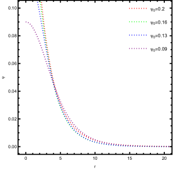
Figure 1: Radial variation of the scalar field for different boson stars, with $\xi=0.05$.

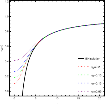
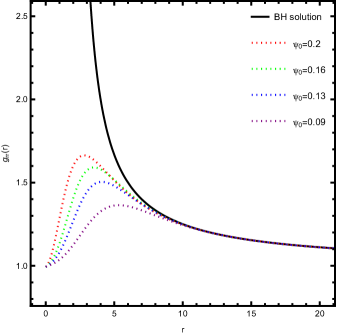
Figure 2: Metric components $-g_{tt}$ (left) and $g_{rr}$ (right) for different boson stars and the Schwarzschild BH, with $\xi=0.05$. The mass of the Schwarzschild BH is set to $1$. The black solid line represents the Schwarzschild BH, while the dotted lines with different colors represent different boson stars.

After obtaining the numerical solutions for the metric components, we can theoretically study the optical image of the boson star using numerical methods. However, due to the presence of infinity in the numerical solutions, we cannot directly use the numerical metric for calculations. Therefore, we employ two specific functions to fit the numerical metric components. The fitting requires minimizing the absolute value of the loss function and ensuring that as $r\to\infty$, the fitted metric asymptotically approaches the Schwarzschild metric. We found that the following functions yield a near-perfect fit

$$g_{tt} =-\exp\left[\alpha_{7}\left(\exp\left(-\frac{1+\alpha_{1}r+\alpha_{2}r^{2}}{\alpha_{3}+\alpha_{4}r+\alpha_{5}r^{2}+\alpha_{6}r^{3}}\right)-1\right)\right],$$ (6.1)

$$g_{rr} =\exp\left[\beta_{7}\left(\exp\left(-\frac{1+\beta_{1}r+\beta_{2}r^{2}}{\beta_{3}+\beta_{4}r+\beta_{5}r^{2}+\beta_{6}r^{3}}\right)-1\right)\right].$$ (6.2)

The fitting results are shown in Figure 3, where the numerical results are represented by dotted lines and the fitting curves are represented by solid lines. It can be observed that for both $-g_{tt}$ and $g_{rr}$, the numerical results almost perfectly coincide with the fitting results. Tables 1 and 2 show the estimated values of the fitting function parameters and the boson star mass $m$ for four initial conditions. It can be observed that as the initial value $\psi_{0}$ increases, the mass $m$ decreases.

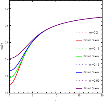
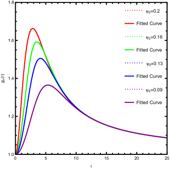
Figure 3: Numerical results and fitting functions of the metric components $-g_{tt}$ (left) and $g_{rr}$ (right) for different boson stars, with $\xi=0.05$. The dotted lines represent the numerical results, while the solid lines represent the fitting functions.

Table 1: Estimated values of the parameters $\alpha_{i}\ (i=1,2,\dots,7)$ in the fitting function $g_{tt}$ (6.1), where $m$ denotes the mass of the boson star, with $\xi=0.05$ fixed.

Type	$\psi_{0}$	$m$	$\alpha_{1}$	$\alpha_{2}$	$\alpha_{3}$	$\alpha_{4}$	$\alpha_{5}$	$\alpha_{6}$	$\alpha_{7}$
BS1	0.2	0.442	0.803	0.33	-0.274	-0.218	0.202	-0.023	-0.061
BS2	0.16	0.528	0.14	0.192	-0.311	-0.046	-0.091	-0.013	-0.071
BS3	0.13	0.581	0.039	0.118	-0.309	-0.014	-0.051	-0.006	-0.055
BS4	0.09	0.625	0.006	0.056	-0.3	-0.003	-0.023	-0.001	-0.033

Table 2: Estimated values of the parameters $\beta_{i}\ (i=1,2,\dots,7)$ in the fitting function $g_{rr}$ (6.2), where $m$ denotes the mass of the boson star, with $\xi=0.05$ fixed.

Type	$\psi_{0}$	$m$	$\beta_{1}$	$\beta_{2}$	$\beta_{3}$	$\beta_{4}$	$\beta_{5}$	$\beta_{6}$	$\beta_{7}$
BS1	0.2	0.442	-30.828	-2.965	2.026	5.501	2.26	0.052	-0.018
BS2	0.16	0.528	-16.192	-2.458	3.725	1.75	1.833	0.068	-0.032
BS3	0.13	0.581	-11.72	-1.71	4.451	0.714	1.314	0.043	-0.033
BS4	0.09	0.625	-8.136	-0.746	4.543	0.319	0.66	0.011	-0.026

We can also plot the effective potential of the boson star as described by equation (4.10). Figure 4 shows the relationship between the effective potential $V_{eff}(r)$ (left subfigure) and its second derivative $[V_{eff}(r)]^{\prime\prime}$ (right subfigure) with respect to the radial distance $r$. It is evident that, unlike the Schwarzschild BH, the effective potential of the boson star decreases monotonically. Due to the absence of an event horizon, the effective potential does not diverge at the right boundary. As indicated by equation (4.11), for the Schwarzschild BH, the second derivative of the effective potential is always less than 0, which signals the formation of a photon ring. However, for the boson star, the second derivative of the effective potential is always greater than 0, implying that the photon motion around the boson star is unstable, preventing the formation of a photon ring, as also illustrated in Figure 6. For both the Schwarzschild BH and the boson star, the effective potential $V_{eff}(r)$ and its second derivative $[V_{eff}(r)]^{\prime\prime}$ exhibit the same asymptotic behavior, as $r\to\infty$, both $V_{eff}(r)\to 0$ and $[V_{eff}(r)]^{\prime\prime}\to 0$.

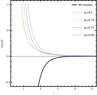
Figure 4: Effective potential $V_{eff}(r)$ (left) and its second derivative $\left[V_{eff}(r)\right]^{\prime\prime}$ (right) for different boson stars and the Schwarzschild BH, with $I=1$ and $\xi=0.05$. The black solid line represents the Schwarzschild BH, while the dotted lines with different colors represent different boson stars.

The optical images of various boson stars illuminated by a spherical light source are presented in Figure 5. In each image, the celestial sphere is divided into four sections, each marked with different colors (red, green, yellow, and blue), with coordinate lines represented by gray lines at intervals of $10^{\degree}$. The boson star is positioned at the center of the celestial sphere with a radius of $r_{\text{obs}}=50m$, while the observer is located at the intersection of the four quadrants. A white reference light source is placed on the opposite side of the celestial sphere relative to the observer, to study the strong gravitational lensing effect and the formation of the Einstein ring. The black transparent region at the center of the image represents the boson star, while the white circle in the outer region represents the Einstein ring.

Several key phenomena are evident from the figures. Since the boson star lacks an event horizon, light entering the boson star is not fully absorbed but is instead partially retained. Similar to a BH, when the light source passes near the boson star, an Einstein ring is formed due to gravitational lensing. Since the boson star is static and does not rotate, its central black region appears as a perfect circle, resembling a non-rotating BH. There is also no frame-dragging effect on the background celestial sphere, as the boson star does not possess angular momentum. Additionally, we investigated the effects of the observation angle $\theta$ and the initial scalar field value $\psi_{0}$ on the optical image. The results show that the observation angle $\theta$ has a minimal impact on the image. However, the initial scalar field value $\psi_{0}$ plays a significant role. As $\psi_{0}$ decreases, both the size of the boson star and the Einstein ring shrink, and the light trajectories inside the Einstein ring also change, highlighting the importance of the scalar field’s initial conditions in determining the optical characteristics of the boson star.

(a) $\psi_{0}=0.2$

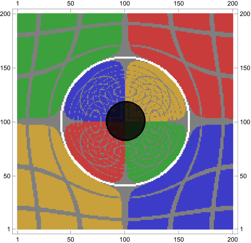
(b) $\psi_{0}=0.16$

(c) $\psi_{0}=0.13$

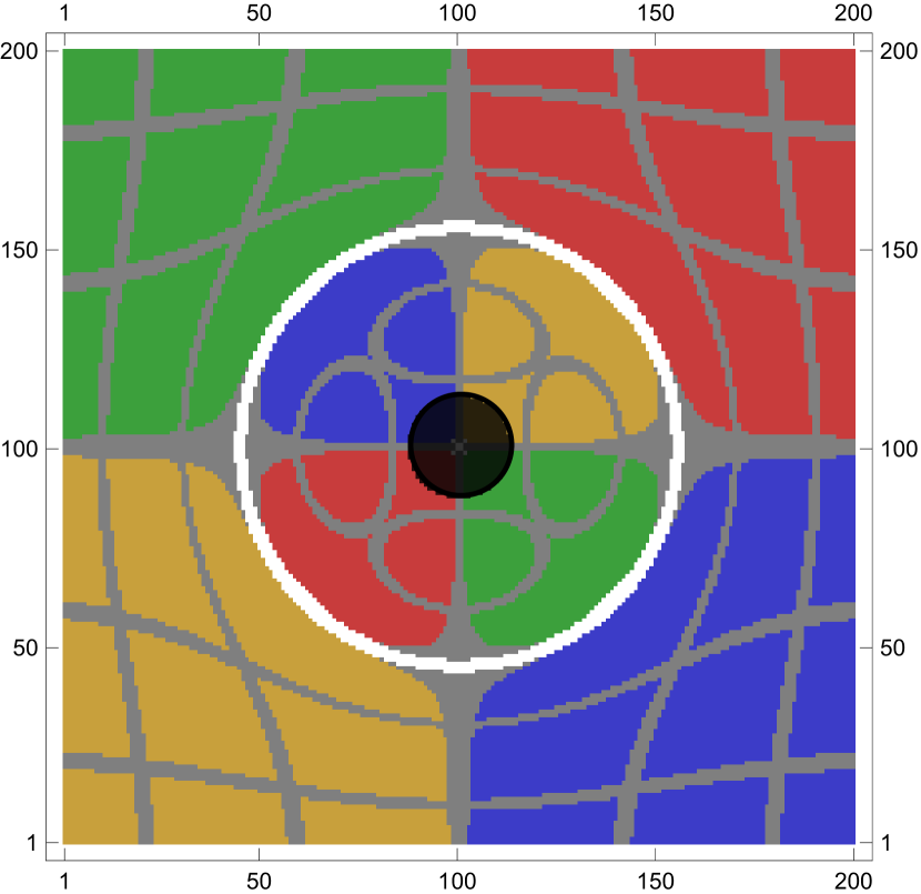
(d) $\psi_{0}=0.09$

Figure 5: Optical images and Einstein rings corresponding to different boson stars under a spherical light source, with $\xi=0.05$, $\alpha_{\text{fov}}=45^{\degree}$, $r_{\text{obs}}=50m$ ($m$ denotes the mass of the boson star), and the inclination angle of the observer is $\theta=45^{\degree}$.

The optical images of various boson stars with a thin accretion disk are presented in Figure 6. In these images, we fix the field-of-view angle $\alpha_{\text{fov}}=3.5^{\degree}$, the gravitational coupling parameter $\xi=0.05$, and place the observer at a distance of $r_{\text{obs}}=200$. The background is represented by orange, with a light intensity of zero, while the colors from yellow to green indicate increasing light intensity, with the boson star at the center of the image.

Several interesting features are observed in these images. When the observation angle $\theta$ is small (e.g., $0^{\degree}$ and $30^{\degree}$ in the first and second columns), the optical image only shows the direct image of the boson star. In this case, the scalar field $\psi_{0}$ primarily influences the size of the direct image, without altering its overall shape. As $\psi_{0}$ decreases, the direct image becomes progressively larger. However, when the observation angle $\theta$ increases (e.g., $60^{\degree}$ and $80^{\degree}$ in the third and fourth columns), the effect of $\psi_{0}$ on the optical image becomes more pronounced, not only affecting the size but also the shape of the direct image. In these cases, lensed images of light are visible in images (c), (d), and (h). For instance, in image (d), the upper hat-shaped optical image represents the direct image ($n=1$), where light passes through the equatorial plane for the first time, while the lower D-shaped image represents the lensed image ($n=2$), where light passes through the equatorial plane for the second time.

At $\theta=0^{\degree}$, the boson star’s optical image appears as a symmetric ring because the observer’s line of sight is perpendicular to the equatorial plane and aligns with the symmetry axis of the accretion disk and the boson star. In this case, the radial velocity of each point on the accretion disk relative to the observer is zero, and the observed redshift is primarily due to gravitational redshift. As the angle $\theta$ increases, the radial velocity’s effect on the observer becomes stronger, leading to an increased Doppler redshift. Detailed analysis reveals that when $\theta\neq 0$, light moving towards the observer experiences a blueshift, which increases photon energy and makes the optical image appear brighter. Conversely, light moving away from the observer undergoes a redshift, reducing photon energy and dimming the optical image. The figures at $\theta=30^{\degree}$, $60^{\degree}$, and $80^{\degree}$ (second, third, and fourth columns) show that the left side of the image is blueshifted, while the right side is redshifted, which is consistent with the results shown in Figure 7.

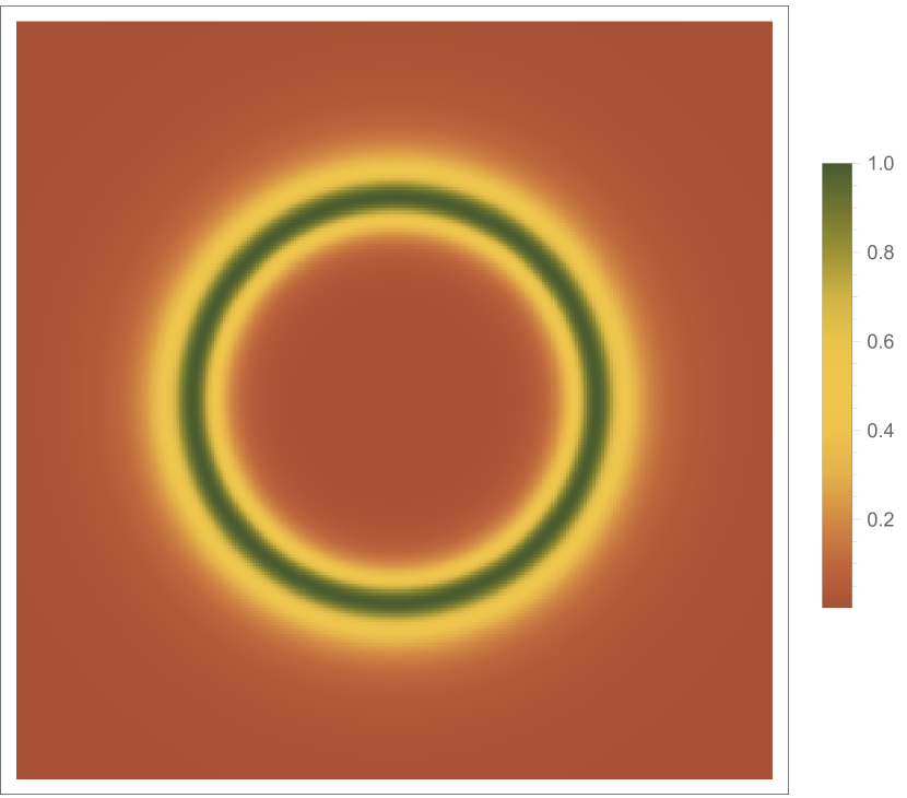
(a) $\psi_{0}=0.2,\theta=0^{\degree}$

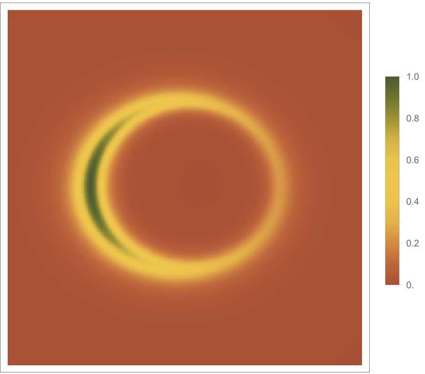
(b) $\psi_{0}=0.2,\theta=30^{\degree}$

(c) $\psi_{0}=0.2,\theta=60^{\degree}$

(d) $\psi_{0}=0.2,\theta=80^{\degree}$

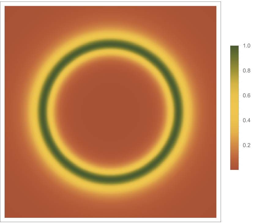
(e) $\psi_{0}=0.16,\theta=0^{\degree}$

(f) $\psi_{0}=0.16,\theta=30^{\degree}$

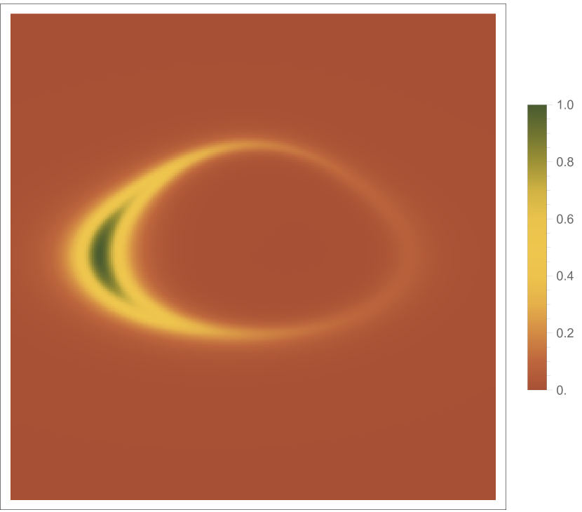
(g) $\psi_{0}=0.16,\theta=60^{\degree}$

(h) $\psi_{0}=0.16,\theta=80^{\degree}$

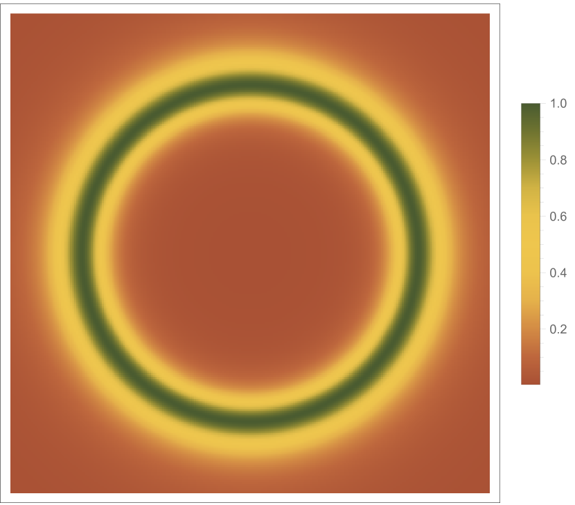
(i) $\psi_{0}=0.13,\theta=0^{\degree}$

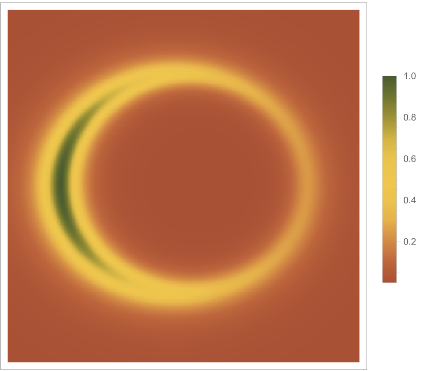
(j) $\psi_{0}=0.13,\theta=30^{\degree}$

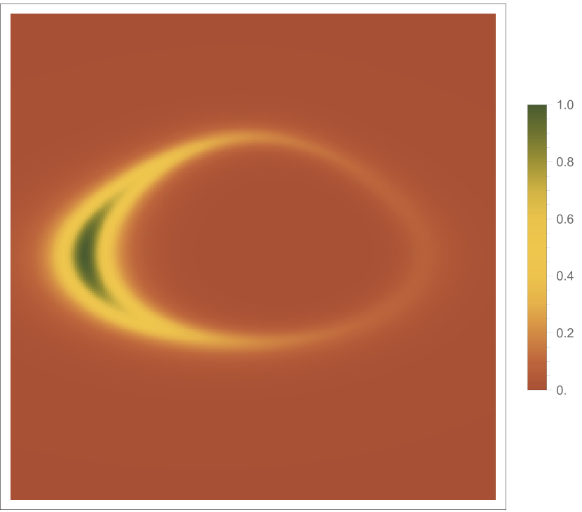
(k) $\psi_{0}=0.13,\theta=60^{\degree}$

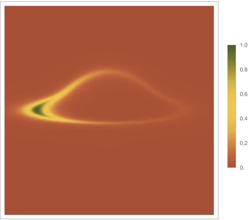
(l) $\psi_{0}=0.13,\theta=80^{\degree}$

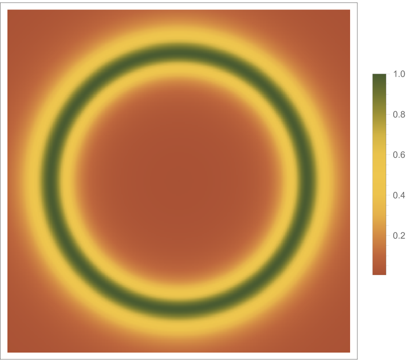
(m) $\psi_{0}=0.09,\theta=0^{\degree}$

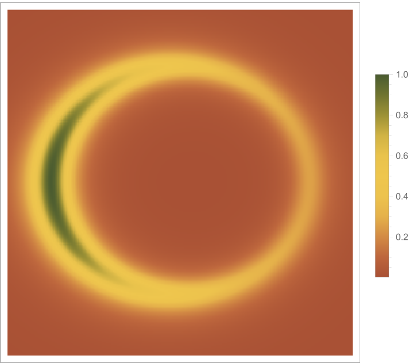
(n) $\psi_{0}=0.09,\theta=30^{\degree}$

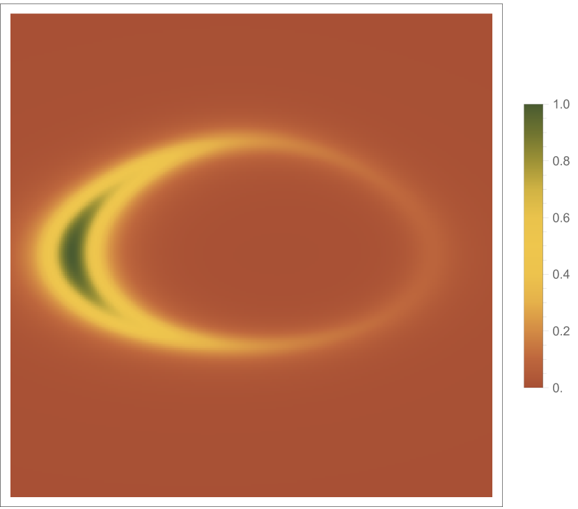
(o) $\psi_{0}=0.09,\theta=60^{\degree}$

(p) $\psi_{0}=0.09,\theta=80^{\degree}$

Figure 6: Optical images corresponding to different boson stars under a thin accretion disk, with $\xi=0.05$ and $\alpha_{\text{fov}}=3.5^{\degree}$. Columns from left to right correspond to models with inclination angle $\theta=0^{\degree},30^{\degree},60^{\degree},80^{\degree}$, and rows from top to bottom correspond to $\psi_{0}=0.2,0.16,0.13,0.09$.

When $n=1$, the light first passes through the equatorial plane, forming the direct image. In this case, the light reaches the observer without significant influence from the gravitational field of the boson star. The corresponding redshift factor distribution for the direct image is shown in Figure 7. We set $\alpha_{\text{fov}}=10^{\degree}$ and $\xi=0.05$. In the figure, red and blue colors represent redshift and blueshift, respectively, with darker colors indicating higher intensity, following a linear relationship. It can be observed that when the observation angle $\theta=0^{\degree}$ (first column), only redshift is present, with no blueshift. As $\psi_{0}$ decreases, the redshift intensity weakens, and its range increases. When $\theta=30^{\degree}$ (second column), a slight blueshift begins to appear. As the observation angle increases further (e.g., $60^{\degree}$ and $80^{\degree}$ in the third and fourth columns), a noticeable blueshift becomes evident in the image. While the redshift intensity weakens as $\psi_{0}$ decreases, the blueshift intensity remains nearly unchanged. By comparing the images in each column, it is evident that for small values of $\theta$, gravitational redshift dominates, whereas for larger values of $\theta$, the radial velocity component of the accreting material increases, leading to enhanced Doppler redshift.

(a) $\psi_{0}=0.2,\theta=0^{\degree}$

(b) $\psi_{0}=0.2,\theta=30^{\degree}$

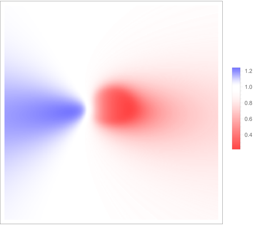
(c) $\psi_{0}=0.2,\theta=60^{\degree}$

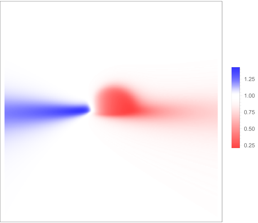
(d) $\psi_{0}=0.2,\theta=80^{\degree}$

(e) $\psi_{0}=0.16,\theta=0^{\degree}$

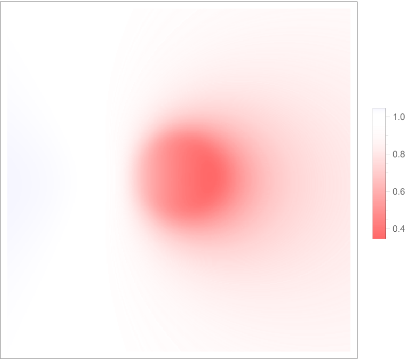
(f) $\psi_{0}=0.16,\theta=30^{\degree}$

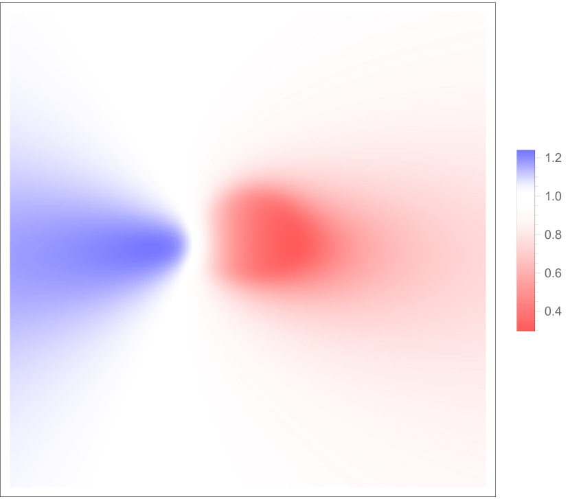
(g) $\psi_{0}=0.16,\theta=60^{\degree}$

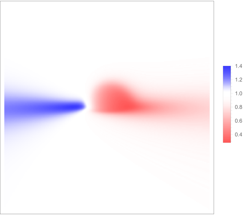
(h) $\psi_{0}=0.16,\theta=80^{\degree}$

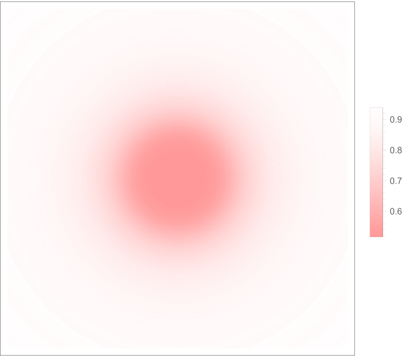
(i) $\psi_{0}=0.13,\theta=0^{\degree}$

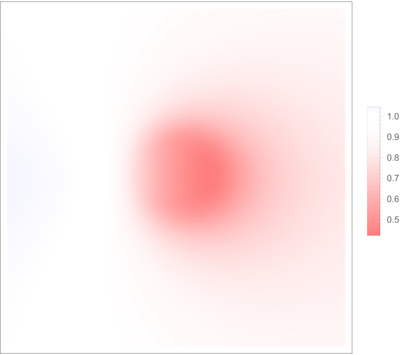
(j) $\psi_{0}=0.13,\theta=30^{\degree}$

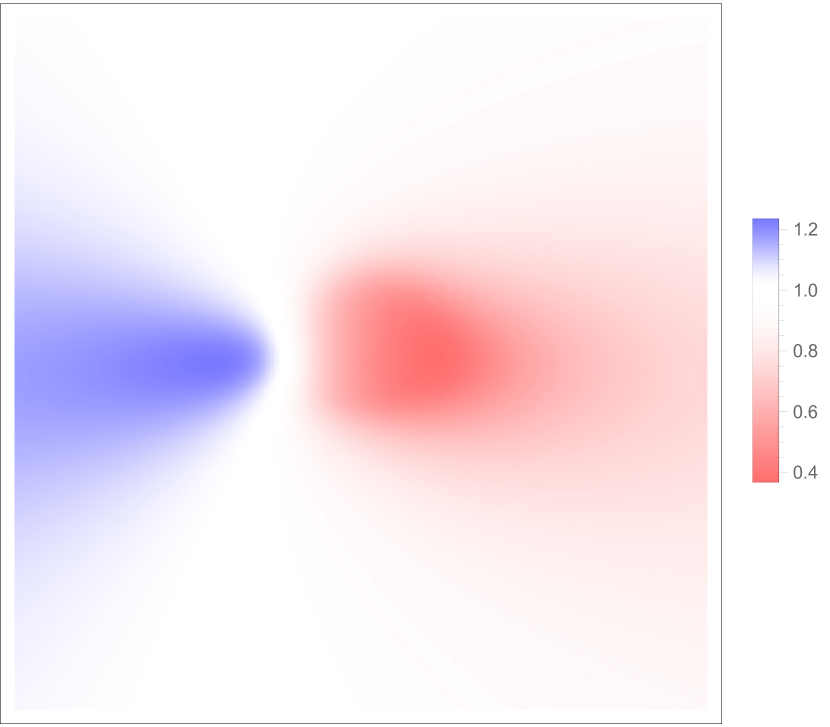
(k) $\psi_{0}=0.13,\theta=60^{\degree}$

(l) $\psi_{0}=0.13,\theta=80^{\degree}$

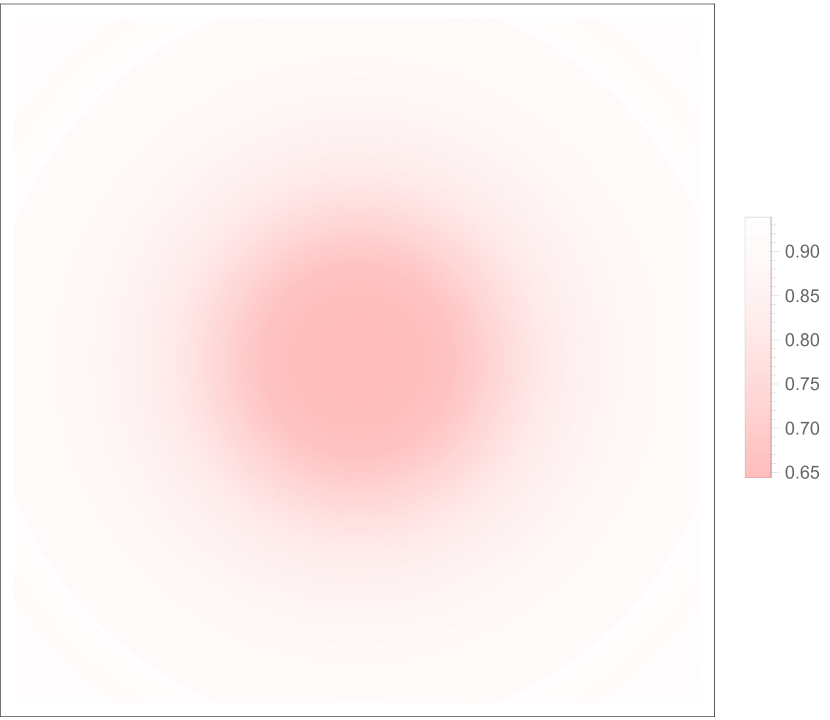
(m) $\psi_{0}=0.09,\theta=0^{\degree}$

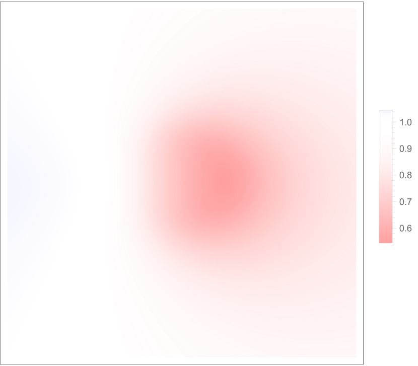
(n) $\psi_{0}=0.09,\theta=30^{\degree}$

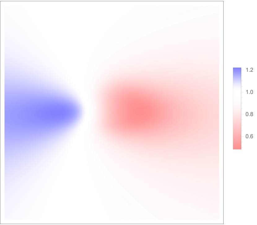
(o) $\psi_{0}=0.09,\theta=60^{\degree}$

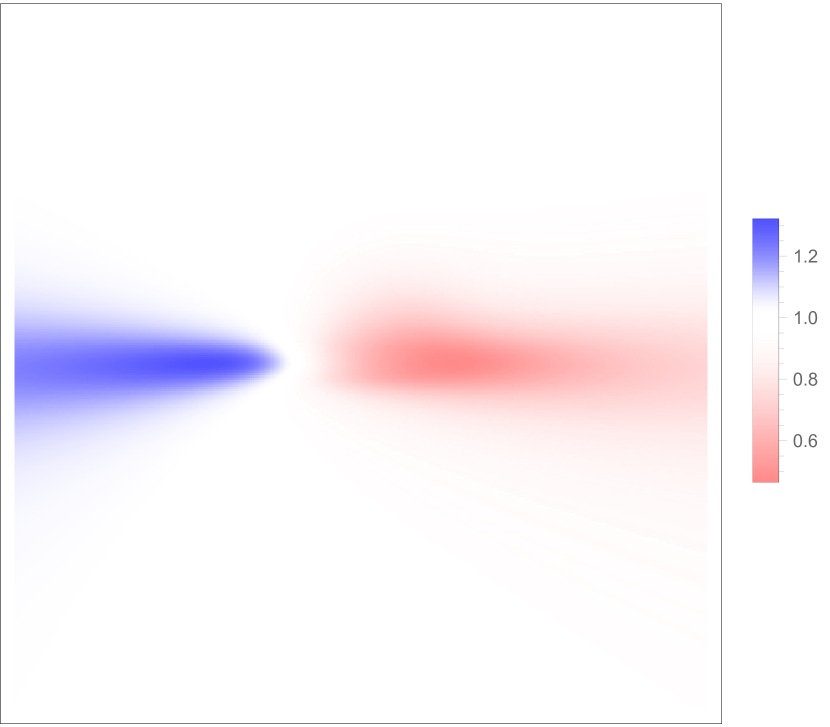
(p) $\psi_{0}=0.09,\theta=80^{\degree}$

Figure 7: Redshift factor distribution corresponding to direct images, with $\xi=0.05$ and $\alpha_{\text{fov}}=10^{\degree}$. The redshift factor is shown using a continuous linear color spectrum, with red for redshift and blue for blueshift. Columns from left to right denote models with inclination angle $\theta=0^{\degree},30^{\degree},60^{\degree},80^{\degree}$, and rows from top to bottom denote $\psi_{0}=0.2,0.16,0.13,0.09$.

6.2 Varying gravitational coupling parameter

In this subsection, we fix the initial scalar field at $\psi_{0}=0.18$ and investigate the impact of the gravitational coupling parameter $\xi$ on the optical images of the boson star. As in the previous subsection, we sequentially compute the numerical solutions for the metric, fit functions, and generate the optical and redshift images.

Figure 8 shows the variation of the scalar field $\psi$ with respect to the radial distance $r$ for different values of the gravitational coupling parameter $\xi$, with the initial scalar field set to $\psi_{0}=0.18$. It can be observed that as the radial distance $r$ increases, the scalar field $\psi$ decreases rapidly, approaching zero as $r\to\infty$. For a fixed value of $r$, an increase in $\xi$ results in a higher value of $\psi$. Figure 9 presents the numerical solutions for the boson star metric components $-g_{tt}$ and $g_{rr}$, with the metric components of the Schwarzschild BH included for comparison. The numerical metric components exhibit similar behavior to those presented in Sec. 6.1, where the metric does not diverge as $r\to 0$, indicating the absence of an event horizon for the boson star. For $r>8M$, the numerical metric components closely match those of the Schwarzschild BH.

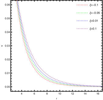
Figure 8: Radial variation of the scalar field for different boson stars, with $\psi_{0}=0.18$.

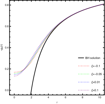
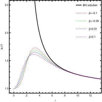
Figure 9: Metric components $-g_{tt}$ (left) and $g_{rr}$ (right) for different boson stars and the Schwarzschild BH, with $\psi_{0}=0.18$. The mass of the Schwarzschild BH is set to $1$. The black solid line represents the Schwarzschild BH, while the dotted lines with different colors represent different boson stars.

The fitting results for the metric components are shown in Figure 10, where the numerical results are represented by dotted lines and the fitting functions are depicted by solid lines. It is evident that for both $-g_{tt}$ and $g_{rr}$, the numerical results closely match the fitting functions, allowing the fitted metric to be used in subsequent calculations. Tables 3 and 4 summarize the estimated values of the fitting function parameters and the boson star mass $m$ for different values of the gravitational coupling parameter $\xi$. It can be observed that as $\xi$ increases, the mass $m$ decreases.

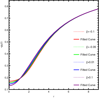
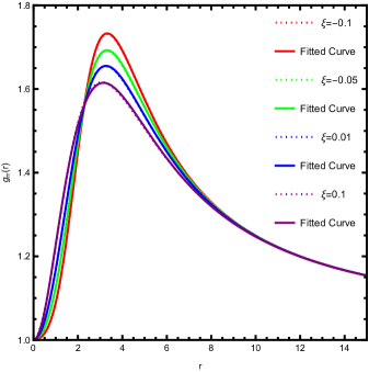
Figure 10: Numerical results and fitting functions of the metric components $-g_{tt}$ (left) and $g_{rr}$ (right) for different boson stars, with $\psi_{0}=0.18$. The dotted lines represent the numerical results, while the solid lines represent the fitting functions.

Table 3: Estimated values of the parameters $\alpha_{i}\ (i=1,2,\dots,7)$ in the fitting function $g_{tt}$ (6.1), where $m$ denotes the mass of the boson star, with $\psi_{0}=0.18$ fixed.

Type	$\xi$	$m$	$\alpha_{1}$	$\alpha_{2}$	$\alpha_{3}$	$\alpha_{4}$	$\alpha_{5}$	$\alpha_{6}$	$\alpha_{7}$
BS1	-0.1	0.56	-0.183	0.341	-0.367	0.061	-0.118	-0.038	-0.125
BS2	-0.05	0.531	-0.049	0.324	-0.356	0.011	-0.128	-0.036	-0.118
BS3	0.01	0.502	0.15	0.287	-0.331	-0.054	-0.136	-0.028	-0.099
BS4	0.1	0.47	0.601	0.234	-0.263	-0.157	-0.132	-0.012	-0.046

Table 4: Estimated values of the parameters $\beta_{i}\ (i=1,2,\dots,7)$ in the fitting function $g_{rr}$ (6.2), where $m$ denotes the mass of the boson star, with $\psi_{0}=0.18$ fixed.

Type	$\xi$	$m$	$\beta_{1}$	$\beta_{2}$	$\beta_{3}$	$\beta_{4}$	$\beta_{5}$	$\beta_{6}$	$\beta_{7}$
BS1	-0.1	0.56	-12.309	-5.858	2.986	-0.085	2.184	0.071	-0.011
BS2	-0.05	0.531	-17.078	-6.108	4.105	0.666	2.874	0.133	-0.022
BS3	0.01	0.502	-19.516	-3.857	3.507	2.172	2.424	0.103	-0.028
BS4	0.1	0.47	-24.078	-1.971	2.314	4.192	1.786	0.038	-0.023

The relationship between the effective potential $V_{eff}(r)$ (left subfigure) and its second derivative $[V_{eff}(r)]^{\prime\prime}$ (right subfigure) with the radial distance $r$ is shown in Figure 11. It can be observed that as $r\to\infty$, both $V_{eff}(r)$ and $[V_{eff}(r)]^{\prime\prime}$ tend to zero. The effective potential of the Schwarzschild BH increases monotonically, with its second derivative always negative; the effective potential of the boson star decreases monotonically, with its second derivative always positive. These differences are reflected in the optical images: for the Schwarzschild BH, a photon ring exists, whereas for the boson star, no photon ring is present.

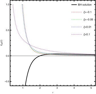
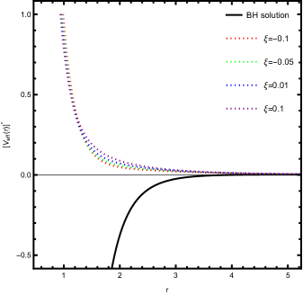
Figure 11: Effective potential $V_{eff}(r)$ (left) and its second derivative $\left[V_{eff}(r)\right]^{\prime\prime}$ (right) for different boson stars and the Schwarzschild BH, with $I=1$ and $\psi_{0}=0.18$. The black solid line represents the Schwarzschild BH, while the dotted lines with different colors represent different boson stars.

The optical images of different boson stars corresponding to a spherical light source are presented in Figure 12. As in the previous discussion, the celestial sphere is divided into four quadrants, with the black transparent region at the center representing the boson star and the white circle in the outer region indicating the Einstein ring. Since the boson star lacks an event horizon, the light within the Einstein ring is not fully absorbed. It is observed that as $\xi$ increases, the sizes of both the boson star and the Einstein ring remain nearly unchanged; however, the light trajectories within the Einstein ring exhibit notable variations. This can be interpreted as a result of changes in the gravitational field near the boson star, induced by variations in $\xi$, which in turn alter the null geodesics.

(a) $\xi=-0.1,\theta=45^{\degree}$

(b) $\xi=-0.05,\theta=45^{\degree}$

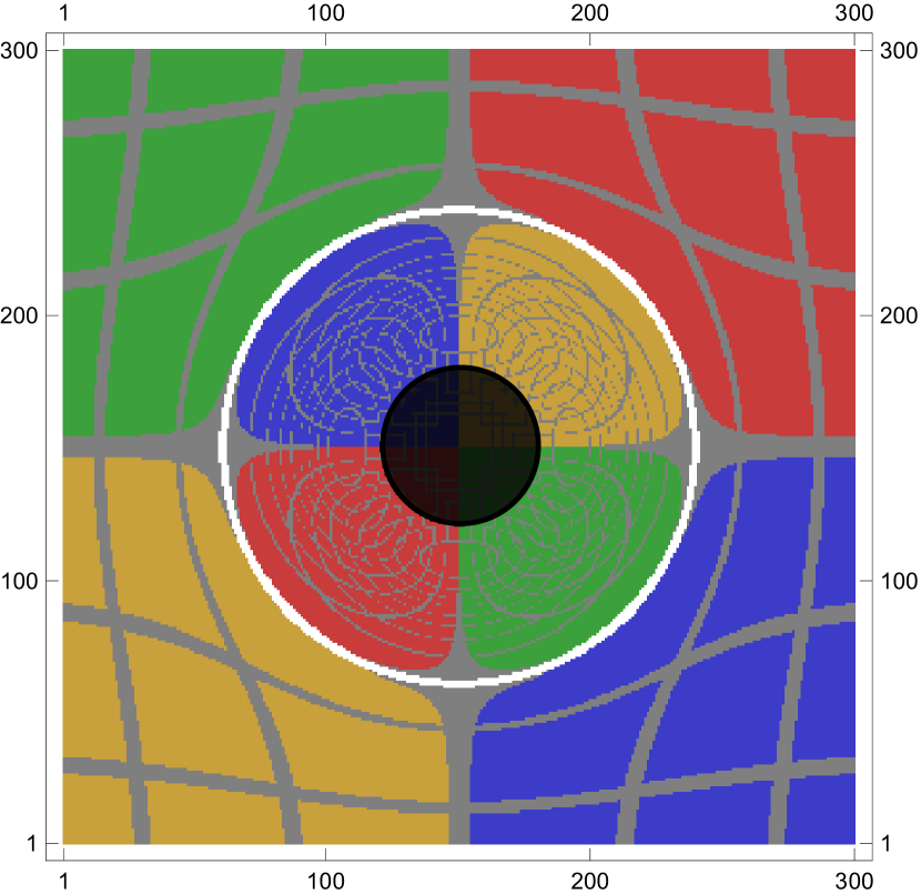
(c) $\xi=0.01,\theta=45^{\degree}$

(d) $\xi=0.1,\theta=45^{\degree}$

Figure 12: Optical images and Einstein rings corresponding to different boson stars under a spherical light source, with $\psi_{0}=0.18$, $\alpha_{\text{fov}}=45^{\degree}$, $r_{\text{obs}}=50m$ ($m$ denotes the mass of the boson star), and the inclination angle of the observer is $\theta=45^{\degree}$.

The optical images of various boson stars with a thin accretion disk are presented in Figure 13. We set $\alpha_{\text{fov}}=2.8^{\degree}$, $\psi_{0}=0.18$, with the observer located at $r_{\text{obs}}=200$. The background is represented in gray, with a light intensity of zero, while the colors ranging from red to white indicate increasing light intensity, with the boson star positioned at the center of the image. It can be observed that for observation angles of $\theta=0^{\degree},30^{\degree},60^{\degree}$ (first, second, and third columns), the optical image displays only a direct image, where $\xi$ affects the size of the direct image but does not alter its shape. As $\xi$ increases, the direct image gradually becomes smaller. When $\theta=86^{\degree}$ (fourth column), a lensed image appears in the optical image of the boson star. The upper hat-shaped optical image corresponds to the direct image, while the lower D-shaped optical image represents the lensed image. As $\xi$ increases, both the direct and lensed images decrease in size. At smaller observation angles, the direct image of the boson star roughly forms a ring, with gravitational redshift dominating. As the observation angle increases, the intensity on the left side of the optical image becomes greater than on the right side, where Doppler redshift dominates. Consequently, blueshift is observed on the left side and redshift on the right side, consistent with the results shown in Figure 14.

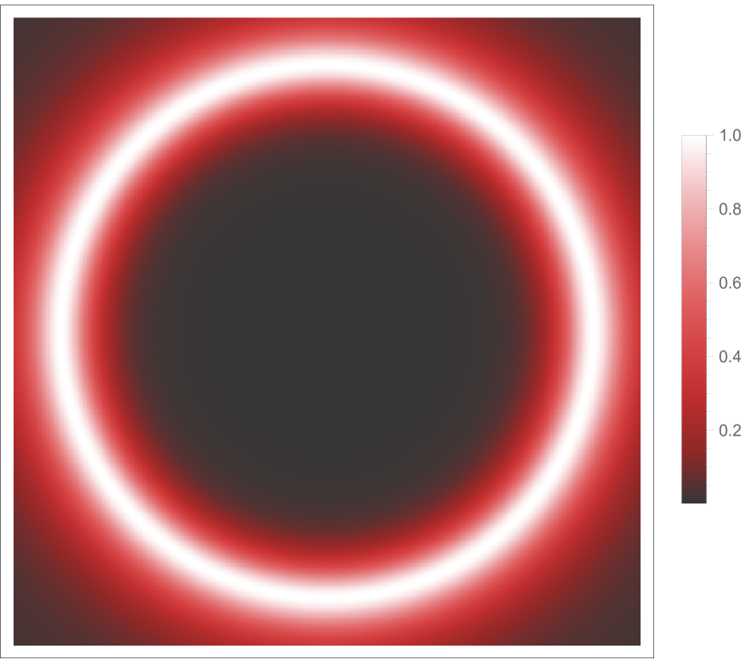
(a) $\xi=-0.1,\theta=0^{\degree}$

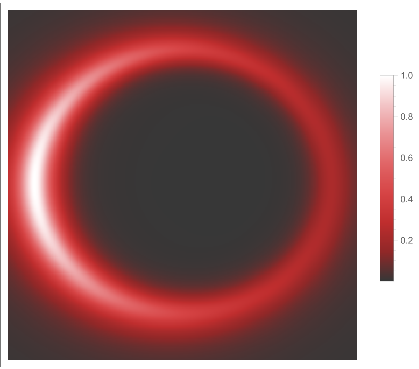
(b) $\xi=-0.1,\theta=30^{\degree}$

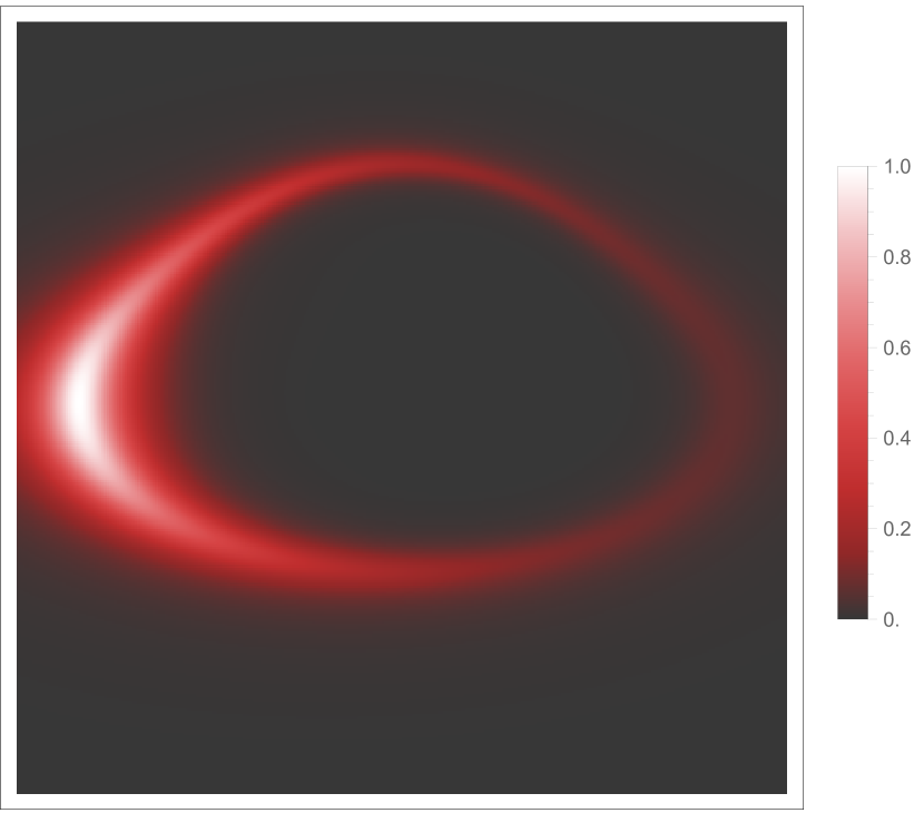
(c) $\xi=-0.1,\theta=60^{\degree}$

(d) $\xi=-0.1,\theta=86^{\degree}$

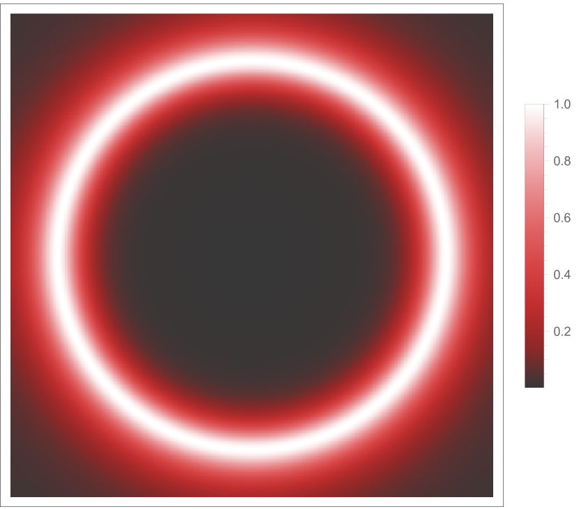
(e) $\xi=-0.05,\theta=0^{\degree}$

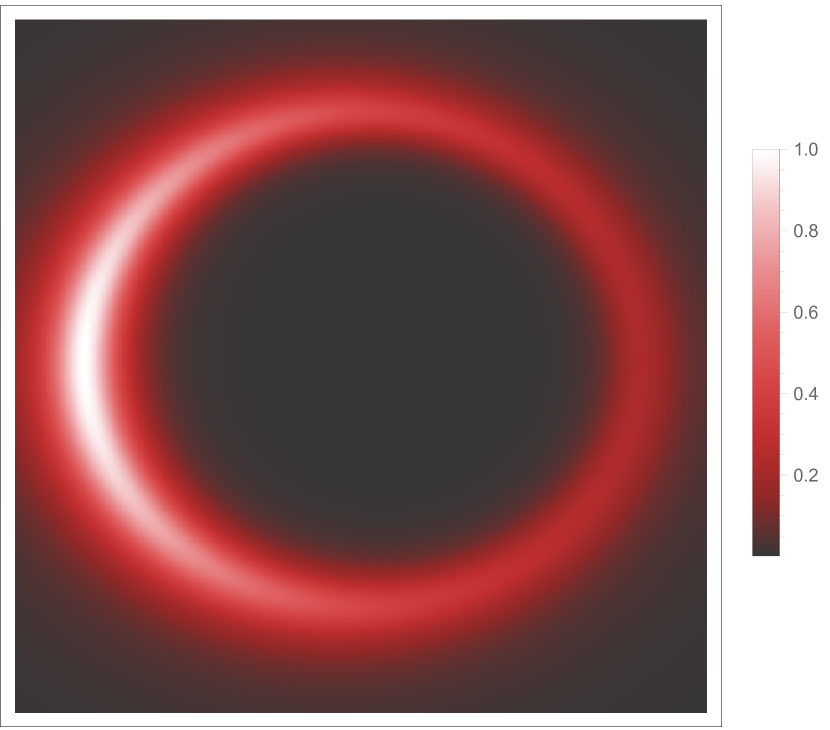
(f) $\xi=-0.05,\theta=30^{\degree}$

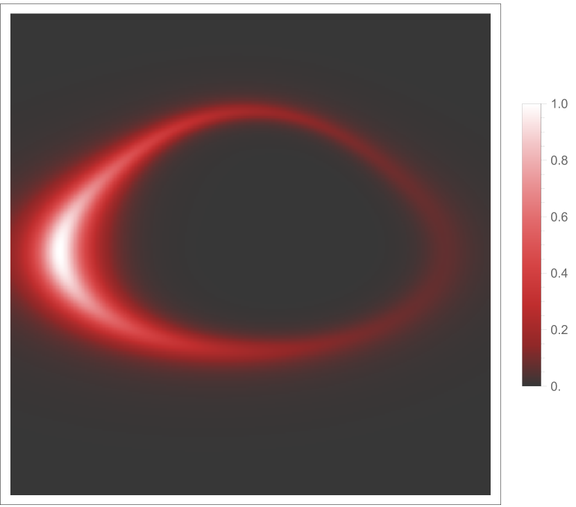
(g) $\xi=-0.05,\theta=60^{\degree}$

(h) $\xi=-0.05,\theta=86^{\degree}$

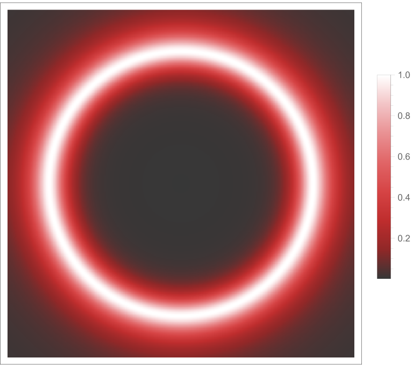
(i) $\xi=0.01,\theta=0^{\degree}$

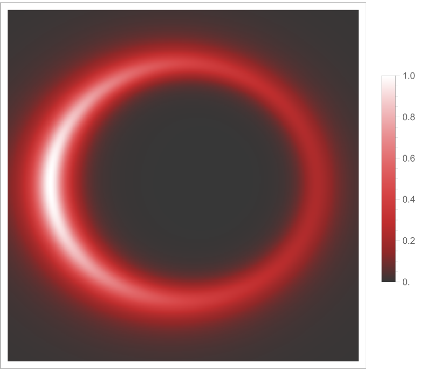
(j) $\xi=0.01,\theta=30^{\degree}$

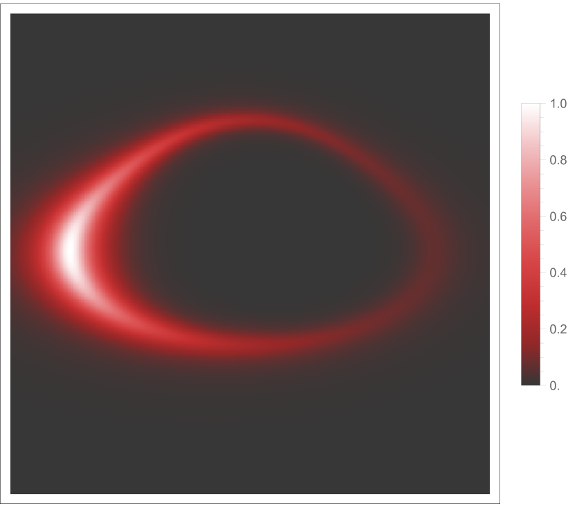
(k) $\xi=0.01,\theta=60^{\degree}$

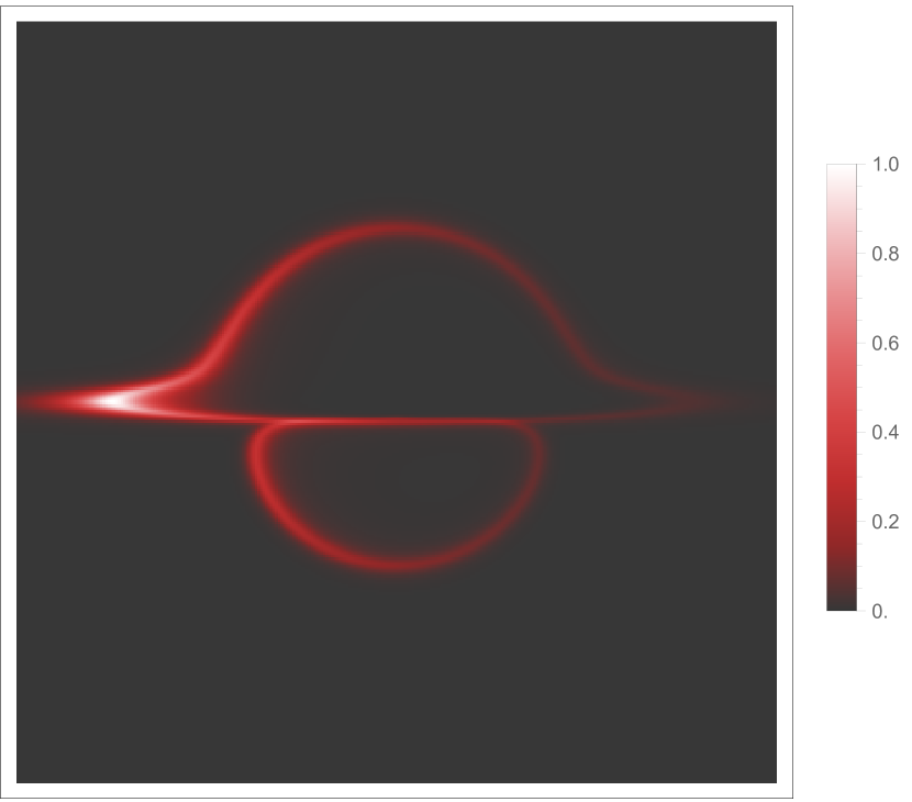
(l) $\xi=0.01,\theta=86^{\degree}$

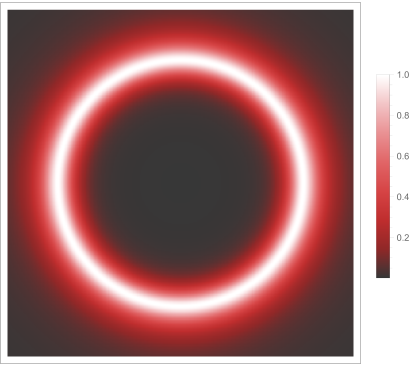
(m) $\xi=0.1,\theta=0^{\degree}$

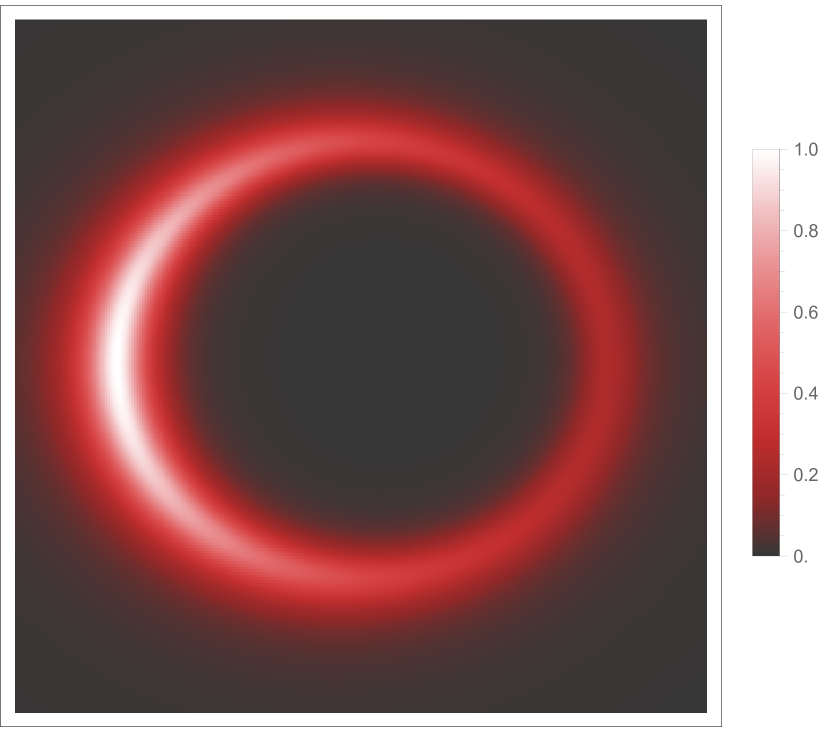
(n) $\xi=0.1,\theta=30^{\degree}$

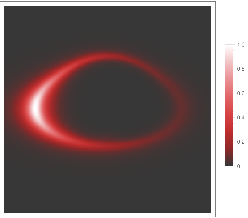
(o) $\xi=0.1,\theta=60^{\degree}$

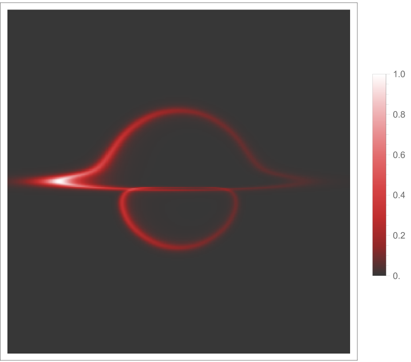
(p) $\xi=0.1,\theta=86^{\degree}$

Figure 13: Optical images corresponding to different boson stars under a thin accretion disk, with $\psi_{0}=0.18$ and $\alpha_{\text{fov}}=2.8^{\degree}$. Columns from left to right correspond to models with inclination angle $\theta=0^{\degree},30^{\degree},60^{\degree},86^{\degree}$, and rows from top to bottom correspond to $\xi=-0.1,-0.05,0.01,0.1$.

The distribution of the redshift factor for the direct image, with light passing through the equatorial plane once for varying values of $\xi$, is shown in Figure 14. We fix $\alpha_{\text{fov}}=10^{\degree}$ and $\psi_{0}=0.18$. By comparing the images in each column, it can be observed that the observation angle $\theta$ has a significant influence on the distribution of redshift and blueshift factors. For small values of $\theta$, the blueshift factor is not prominent. As $\theta$ increases, the blueshift factor gradually becomes more noticeable, and the distribution of both blueshift and redshift factors transitions from being scattered to more concentrated. This phenomenon can be explained in accordance with the reasoning provided earlier. By comparing the images in each row, it is found that $\xi$ has little effect on the overall distribution of redshift and blueshift factors. However, it is notable that in the fourth column ($\theta=86^{\degree}$), as $\xi$ increases, the variation in the blueshift factor becomes more concentrated.

(a) $\xi=-0.1,\theta=0^{\degree}$

(b) $\xi=-0.1,\theta=30^{\degree}$

(c) $\xi=-0.1,\theta=60^{\degree}$

(d) $\xi=-0.1,\theta=86^{\degree}$

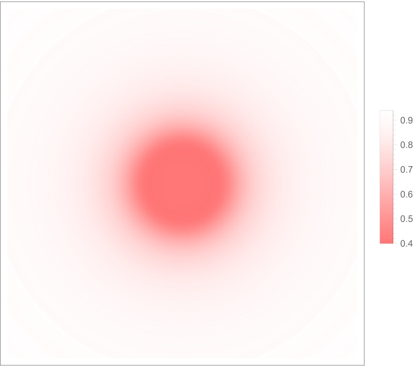
(e) $\xi=-0.05,\theta=0^{\degree}$

(f) $\xi=-0.05,\theta=30^{\degree}$

(g) $\xi=-0.05,\theta=60^{\degree}$

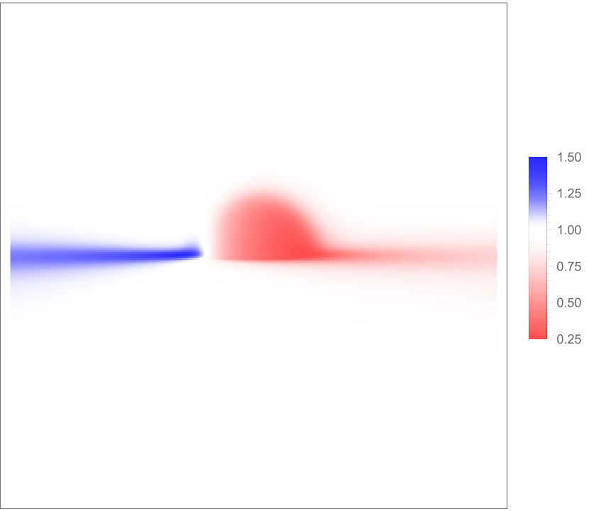
(h) $\xi=-0.05,\theta=86^{\degree}$

(i) $\xi=0.01,\theta=0^{\degree}$

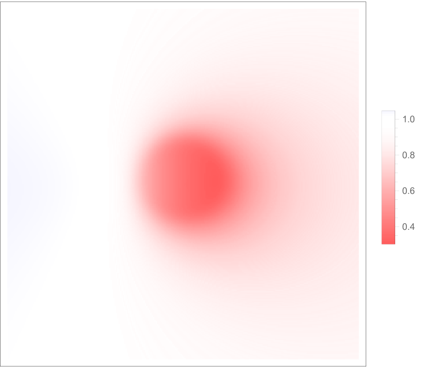
(j) $\xi=0.01,\theta=30^{\degree}$

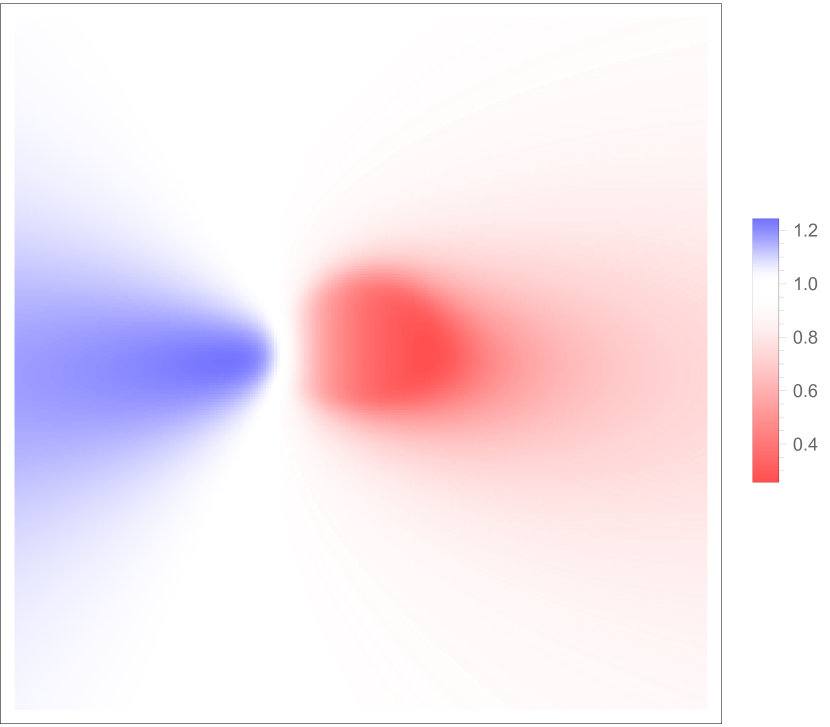
(k) $\xi=0.01,\theta=60^{\degree}$

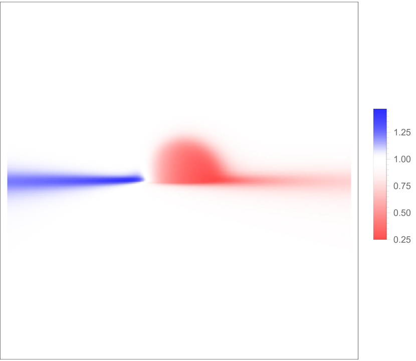
(l) $\xi=0.01,\theta=86^{\degree}$

(m) $\xi=0.1,\theta=0^{\degree}$

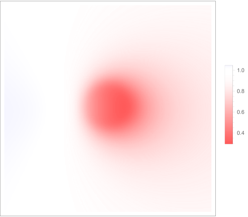
(n) $\xi=0.1,\theta=30^{\degree}$

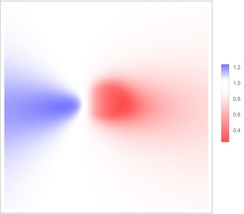
(o) $\xi=0.1,\theta=60^{\degree}$

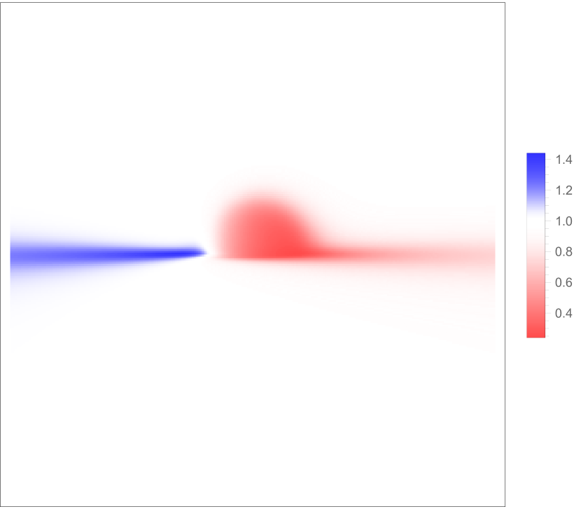
(p) $\xi=0.1,\theta=86^{\degree}$

Figure 14: Redshift factor distribution corresponding to direct images, with $\psi_{0}=0.18$ and $\alpha_{\text{fov}}=10^{\degree}$. The redshift factor is shown using a continuous linear color spectrum, with red for redshift and blue for blueshift. Columns from left to right denote models with inclination angle $\theta=0^{\degree},30^{\degree},60^{\degree},86^{\degree}$, and rows from top to bottom denote $\xi=-0.1,-0.05,0.01,0.1$.

7 Conclusion and discussion

In this work, we have investigated the optical properties of mini boson stars within the framework of Palatini $f(R)$ gravity, adopting the quadratic form $f(R)=R+\xi R^{2}$. By numerically solving the modified field equations, we have analyzed photon trajectories and optical images generated under spherical light sources and thin accretion disks. Our results reveal several key distinctions between boson stars and Schwarzschild black holes, offering theoretical insights into the astrophysical observability of exotic compact objects.

First, we find that boson stars lack stable photon rings due to the positive second derivative of their effective potential, in stark contrast to the negative second derivative observed in Schwarzschild black holes. This characteristic leads to optical images of boson stars being dominated by direct emissions from photons completing a single orbit. The absence of photon rings results in distinctive imaging features that can serve as observational signatures.

Second, we have demonstrated that the optical characteristics of boson stars are highly sensitive to the initial scalar field $\psi_{0}$ and the gravitational coupling parameter $\xi$. Variations in $\psi_{0}$ significantly affect the size of the boson star and the corresponding Einstein ring, while changes in $\xi$ influence the effective potential and redshift distributions. These dependencies highlight the critical role of model parameters in determining the observational properties of boson stars.

Our findings underscore the importance of high-resolution observations for distinguishing boson stars from black holes. The unique optical features of boson stars, such as the absence of photon rings and the specific redshift patterns, provide a promising pathway for probing the existence of exotic compact objects. Moreover, the use of Palatini $f(R)$ gravity in this context extends the applicability of modified gravity theories to compact astrophysical systems, offering an alternative to general relativity for exploring deviations in strong-field regimes.

Future research directions include extending the current analysis to include rotating boson stars and exploring the impact of higher-order terms in the $f(R)$ function. Additionally, incorporating more realistic accretion disk models and analyzing multi-wavelength observations could further refine the distinguishability of boson stars from black holes. These efforts will enhance our understanding of exotic compact objects and contribute to the broader quest for observational tests of alternative gravity theories.

References

- [1] L.S. Collaboration, V. Collaboration et al., Gwtc-1: A gravitational-wave transient catalog of compact binary mergers observed by ligo and virgo during the first and second observing runs, .
- [2] R. Abbott, T. Abbott, S. Abraham, F. Acernese, K. Ackley, A. Adams et al., Gwtc-2: compact binary coalescences observed by ligo and virgo during the first half of the third observing run, Physical Review X 11 (2021) 021053.
- [3] R. Abbott, T. Abbott, S. Abraham, F. Acernese, K. Ackley, C. Adams et al., Gw190814: Gravitational waves from the coalescence of a 23 solar mass black hole with a 2.6 solar mass compact object, The Astrophysical Journal Letters 896 (2020) L44.
- [4] R. Abbott, T. Abbott, S. Abraham, F. Acernese, K. Ackley, C. Adams et al., Gw190521: a binary black hole merger with a total mass of 150 , Physical review letters 125 (2020) 101102.
- [5] R. Abbott, T. Abbott, S. Abraham, F. Acernese, K. Ackley, C. Adams et al., Properties and astrophysical implications of the 150 binary black hole merger gw190521, The Astrophysical Journal Letters 900 (2020) L13.
- [6] V. De Luca, V. Desjacques, G. Franciolini, P. Pani and A. Riotto, Gw190521 mass gap event and the primordial black hole scenario, Physical review letters 126 (2021) 051101.
- [7] J.C. Bustillo, N. Sanchis-Gual, A. Torres-Forné, J.A. Font, A. Vajpeyi, R. Smith et al., Gw190521 as a merger of proca stars: a potential new vector boson of 8.7 10-13 ev, Physical Review Letters 126 (2021) 081101.
- [8] V. Cardoso and P. Pani, Testing the nature of dark compact objects: a status report, Living Reviews in Relativity 22 (2019) 4.
- [9] C.A. Herdeiro, A.M. Pombo, E. Radu, P.V. Cunha and N. Sanchis-Gual, The imitation game: Proca stars that can mimic the schwarzschild shadow, Journal of Cosmology and Astroparticle Physics 2021 (2021) 051.
- [10] D.J. Kaup, Klein-gordon geon, Physical Review 172 (1968) 1331.
- [11] R. Ruffini and S. Bonazzola, Systems of self-gravitating particles in general relativity and the concept of an equation of state, Physical Review 187 (1969) 1767.
- [12] S.L. Liebling and C. Palenzuela, Dynamical boson stars, Living Reviews in Relativity 26 (2023) 1.
- [13] F. Di Giovanni, N. Sanchis-Gual, P. Cerdá-Durán, M. Zilhão, C. Herdeiro, J.A. Font et al., Dynamical bar-mode instability in spinning bosonic stars, Physical Review D 102 (2020) 124009.
- [14] C. Palenzuela, I. Olabarrieta, L. Lehner and S.L. Liebling, Head-on collisions of boson stars, Physical Review D—Particles, Fields, Gravitation, and Cosmology 75 (2007) 064005.
- [15] C. Palenzuela, L. Lehner and S.L. Liebling, Orbital dynamics of binary boson star systems, Physical Review D—Particles, Fields, Gravitation, and Cosmology 77 (2008) 044036.
- [16] F.E. Schunck and E.W. Mielke, Rotating boson star as an effective mass torus in general relativity, Physics Letters A 249 (1998) 389.
- [17] S. Yoshida and Y. Eriguchi, Rotating boson stars in general relativity, Physical Review D 56 (1997) 762.
- [18] B. Kleihaus, J. Kunz, M. List and I. Schaffer, Rotating boson stars and q-balls. ii. negative parity and ergoregions, Physical Review D—Particles, Fields, Gravitation, and Cosmology 77 (2008) 064025.
- [19] M. Bezares, C. Palenzuela and C. Bona, Final fate of compact boson star mergers, Physical Review D 95 (2017) 124005.
- [20] C. Palenzuela, P. Pani, M. Bezares, V. Cardoso, L. Lehner and S. Liebling, Gravitational wave signatures of highly compact boson star binaries, Physical Review D 96 (2017) 104058.
- [21] F. Vincent, Z. Meliani, P. Grandclément, E. Gourgoulhon and O. Straub, Imaging a boson star at the galactic center, Classical and Quantum Gravity 33 (2016) 105015.
- [22] J.L. Rosa and D. Rubiera-Garcia, Shadows of boson and proca stars with thin accretion disks, Physical Review D 106 (2022) 084004.
- [23] J.L. Rosa, C.F. Macedo and D. Rubiera-Garcia, Imaging compact boson stars with hot spots and thin accretion disks, Physical Review D 108 (2023) 044021.
- [24] F.S. Guzmán, Accretion disk onto boson stars: A way to supplant black hole candidates, Physical Review D—Particles, Fields, Gravitation, and Cosmology 73 (2006) 021501.
- [25] H. Olivares, Z. Younsi, C.M. Fromm, M. De Laurentis, O. Porth, Y. Mizuno et al., How to tell an accreting boson star from a black hole, Monthly Notices of the Royal Astronomical Society 497 (2020) 521.
- [26] X.-X. Zeng, L.-F. Li, P. Li, B. Liang and P. Xu, Holographic images of a charged black hole in lorentz symmetry breaking massive gravity, Science China Physics, Mechanics & Astronomy 68 (2025) 220412.
- [27] S. Guo, Y.-X. Huang, E.-W. Liang, Y. Liang, Q.-Q. Jiang and K. Lin, Image of the kerr–newman black hole surrounded by a thin accretion disk, The Astrophysical Journal 975 (2024) 237.
- [28] Y.-H. Cui, S. Guo, Y.-X. Huang, Y. Liang and K. Lin, Optical appearance of numerical black hole solutions in higher derivative gravity, The European Physical Journal C 84 (2024) 772.
- [29] S. Guo, Y.-X. Huang, K. Liu, E.-W. Liang and K. Lin, Influence of quantum correction on the schwarzschild black hole polarized image, The European Physical Journal C 84 (2024) 601.
- [30] K.-J. He, Z. Luo, S. Guo and G.-P. Li, Observational appearance and extra photon rings of an asymmetric thin-shell wormhole with a bardeen profile, Chinese Physics C 48 (2024) 065105.
- [31] Y. Hou, J. Huang, Y. Mizuno, M. Guo and B. Chen, Unique imprint of black hole spin on the polarization of near-horizon images, arXiv preprint arXiv:2409.07248 (2024) .
- [32] J. Huang, Z. Zhang, M. Guo and B. Chen, Images and flares of geodesic hot spots around a kerr black hole, Physical Review D 109 (2024) 124062.
- [33] Z. Zhang, Y. Hou, M. Guo and B. Chen, Imaging thick accretion disks and jets surrounding black holes, Journal of Cosmology and Astroparticle Physics 2024 (2024) 032.
- [34] X.-X. Zeng, H.-Q. Zhang and H. Zhang, Shadows and photon spheres with spherical accretions in the four-dimensional gauss–bonnet black hole, The European Physical Journal C 80 (2020) 1.
- [35] C.-Y. Yang, M.I. Aslam, X.-X. Zeng and R. Saleem, Shadow images of ghosh-kumar rotating black hole illuminated by spherical light sources and thin accretion disks, arXiv preprint arXiv:2411.11807 (2024) .
- [36] X.-X. Zeng, G.-P. Li and K.-J. He, The shadows and observational appearance of a noncommutative black hole surrounded by various profiles of accretions, Nuclear Physics B 974 (2022) 115639.
- [37] G.J. Olmo, Palatini approach to modified gravity: f (r) theories and beyond, International Journal of Modern Physics D 20 (2011) 413.
- [38] T. Harko and F.S. Lobo, Extensions of f (R) Gravity: Curvature-Matter Couplings and Hybrid Metric-Palatini Theory, vol. 1, Cambridge University Press (2018).
- [39] A. Maso-Ferrando, N. Sanchis-Gual, J.A. Font and G.J. Olmo, Boson stars in palatini gravity, arXiv preprint arXiv:2103.15705 (2021) .
- [40] G.J. Olmo, D. Rubiera-Garcia and A. Wojnar, Stellar structure models in modified theories of gravity: Lessons and challenges, Physics Reports 876 (2020) 1.
- [41] D.F. Torres, A.R. Liddle and F.E. Schunck, Gravitational memory of boson stars, Physical Review D 57 (1998) 4821.
- [42] Y. Brihaye, A. Cisterna and C. Erices, Boson stars in biscalar extensions of horndeski gravity, Physical Review D 93 (2016) 124057.
- [43] B. Hartmann, J. Riedel and R. Suciu, Gauss–bonnet boson stars, Physics Letters B 726 (2013) 906.
- [44] F.W. Hehl, J.D. McCrea, E.W. Mielke and Y. Ne’eman, Metric-affine gauge theory of gravity: field equations, noether identities, world spinors, and breaking of dilation invariance, Physics Reports 258 (1995) 1.
- [45] J. Beltran Jimenez, L. Heisenberg and T.S. Koivisto, The geometrical trinity of gravity, Universe 5 (2019) 173.
- [46] V.I. Afonso, G.J. Olmo, E. Orazi and D. Rubiera-Garcia, Correspondence between modified gravity and general relativity with scalar fields, Physical Review D 99 (2019) 044040.
- [47] A. Delhom, G.J. Olmo and E. Orazi, Ricci-based gravity theories and their impact on maxwell and nonlinear electromagnetic models, Journal of High Energy Physics 2019 (2019) 1.
- [48] V.I. Afonso, G.J. Olmo, E. Orazi and D. Rubiera-Garcia, Mapping nonlinear gravity into general relativity with nonlinear electrodynamics, The European Physical Journal C 78 (2018) 1.
- [49] V. Afonso, G.J. Olmo and D. Rubiera-Garcia, Mapping ricci-based theories of gravity into general relativity, Physical Review D 97 (2018) 021503.
- [50] V.I. Afonso, G.J. Olmo, E. Orazi and D. Rubiera-Garcia, New scalar compact objects in ricci-based gravity theories, Journal of Cosmology and Astroparticle Physics 2019 (2019) 044.
- [51] C.A. Herdeiro, A.M. Pombo and E. Radu, Asymptotically flat scalar, dirac and proca stars: discrete vs. continuous families of solutions, Physics Letters B 773 (2017) 654.
- [52] G.J. Olmo, The gravity lagrangian according to solar system experiments, Physical review letters 95 (2005) 261102.
- [53] P. Avelino, Eddington-inspired born-infeld gravity: nuclear physics constraints and the validity of the continuous fluid approximation, Journal of Cosmology and Astroparticle Physics 2012 (2012) 022.
- [54] J.B. Jiménez, L. Heisenberg, G.J. Olmo and D. Rubiera-Garcia, Born–infeld inspired modifications of gravity, Physics Reports 727 (2018) 1.
- [55] J. Näf and P. Jetzer, On the 1/c expansion of f (r) gravity, Physical Review D—Particles, Fields, Gravitation, and Cosmology 81 (2010) 104003.
- [56] S.E. Gralla, A. Lupsasca and D.P. Marrone, The shape of the black hole photon ring: A precise test of strong-field general relativity, Physical Review D 102 (2020) 124004.
- [57] F.H. Vincent, S.E. Gralla, A. Lupsasca and M. Wielgus, Images and photon ring signatures of thick disks around black holes, Astronomy & Astrophysics 667 (2022) A170.