On Deciding the Data Complexity of Answering Linear Monadic Datalog Queries with LTL Operators (Extended Version)

Abstract

Our concern is the data complexity of answering linear monadic datalog queries whose atoms in the rule bodies can be prefixed by operators of linear temporal logic L​TL. We first observe that, for data complexity, answering any connected query with operators $\bigcirc$/$\raisebox{1.07639pt}{\text{\scriptsize{$\bigcirc$}}}^{-}$ (at the next/previous moment) is either in $\textsc{AC}^{0}$, or in ${\textsc{ACC}^{0}}\!\setminus\!{\textsc{AC}^{0}}$, or $\textsc{NC}^{1}$-complete, or L-hard and in NL. Then we show that the problem of deciding L-hardness of answering such queries is PSpace-complete, while checking membership in the classes $\textsc{AC}^{0}$ and $\textsc{ACC}^{0}$ as well as $\textsc{NC}^{1}$-completeness can be done in ExpSpace. Finally, we prove that membership in $\textsc{AC}^{0}$ or in $\textsc{ACC}^{0}$, $\textsc{NC}^{1}$-completeness, and L-hardness are undecidable for queries with operators $\Diamond$/$\raisebox{0.43057pt}{\text{\small{$\Diamond$}}}\!^{-}$ (sometime in the future/past) provided that ${\textsc{NC}^{1}}\neq\textsc{NL}$ and $\textsc{L}\neq\textsc{NL}$.

1 Introduction

We consider monadic datalog queries, in which atoms in the rule bodies can be prefixed by the temporal operators $\bigcirc$/${\raisebox{1.07639pt}{\text{\scriptsize{$\bigcirc$}}}^{-}}$ (at the next/previous moment) and $\Diamond$/$\raisebox{0.43057pt}{\text{\small{$\Diamond$}}}\!^{-}$ (sometime in the future/past) of linear temporal logic L​TL [16]. This query language, denoted $\textsl{datalog}_{m}^{\,\scriptscriptstyle\bigcirc{\smash{\raisebox{-1.3pt}{$\diamond$}}}}$, is intended for querying temporal graph databases and knowledge graphs in scenarios such as virus transmission [24, 47], transport networks [27], social media [40], supply chains [48], and power grids [38]. In this setting, data instances are finite sets of ground atoms that are timestamped by the moments of time they happen at. The rules in $\textsl{datalog}_{m}^{\,\scriptscriptstyle\bigcirc{\smash{\raisebox{-1.3pt}{$\diamond$}}}}$ queries are assumed to hold at all times, with time being implicit in the rules and only accessible via temporal operators. We choose L​TL for our formalism rather than, say, more expressive metric temporal logic MTL [29, 1] because L​TL has been a well established query language in temporal databases since the 1990s (see [41, 43, 13, 32] and the discussion therein on point versus interval-based query languages), also suitable in the context of temporal knowledge graphs as recently argued in [18].

Example 1.1.

Imagine a PhD student working on a paper while hostel hopping. However, finishing the paper requires staying at the same hostel for at least two consecutive nights. Bus services between hostels, which vary from one day to the next, and hostel vacancies are given by a temporal data instance with atoms of the form $\textit{busService}(a,b,n)$ and $\textit{Vacant}(a,n)$, where $a$, $b$ are hostels and $n\in\mathbb{N}$ a timestamp (see Fig. 1 for an illustration). The following $\textsl{datalog}_{m}^{\,\scriptscriptstyle\bigcirc{\smash{\raisebox{-1.3pt}{$\diamond$}}}}$ query $(\pi_{1},\textit{Success})$ finds pairs $(x,t)$ such that having started hopping at hostel $x$ on day $t$, the student will eventually submit the paper:

$$\pi_{1}\colon\quad\begin{split}&\textit{Success}(X)\leftarrow\textit{Vacant}(X)\land{\raisebox{1.07639pt}{\text{\scriptsize{$\bigcirc$}}}}\textit{busService}(X,Y)\wedge{\raisebox{1.07639pt}{\text{\scriptsize{$\bigcirc$}}}}\textit{Success}(Y),\\ &\textit{Success}(X)\leftarrow\textit{Vacant}(X)\land{\raisebox{1.07639pt}{\text{\scriptsize{$\bigcirc$}}}}\textit{Vacant}(X).\end{split}$$

It is readily seen that answering this query is NL-complete for data complexity. If, however, we drop the next-time operator $\bigcirc$ from $\pi_{1}$, it will become equivalent to $\textit{Vacant}(X)$. The next query $(\pi_{2},\textit{Promising})$ simply looks for pairs $(x,t)$ with $x$ having vacancies for two consecutive nights some time later than $t$:

$$\pi_{2}\colon\quad\begin{split}&\textit{Promising}(X)\leftarrow\raisebox{0.43057pt}{\text{\small{$\Diamond$}}}\textit{Vacant42Nights}(X),\\ &\textit{Vacant42Nights}(X)\leftarrow\textit{Vacant}(X)\land{\raisebox{1.07639pt}{\text{\scriptsize{$\bigcirc$}}}}\textit{Vacant}(X).\end{split}$$

This $\textsl{datalog}_{m}^{\,\scriptscriptstyle\bigcirc{\smash{\raisebox{-1.3pt}{$\diamond$}}}}$ query can be equivalently expressed as the two-sorted first-order formula

$$\exists t^{\prime}\,\big{(}(t<t^{\prime})\wedge\textit{Vacant}(x,t^{\prime})\wedge\textit{Vacant}(x,t^{\prime}+1)\big{)},$$

where $x$ ranges over objects (hostels) and $t,t^{\prime}$ over time points ordered by $<$. Formulas in such a two-sorted first-order logic, denoted $\textup{FO}(<)$, can be evaluated over finite data instances in $\textsc{AC}^{0}$ for data complexity [25]. $\dashv$

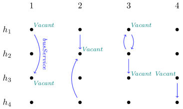
(a) Hostels $h_{1},h_{2},h_{3},h_{4}$ on days $1,2,3,4$.

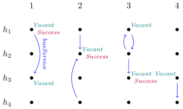
(b) Predicate Success inferred by the program $\pi_{1}$.

Figure 1: Illustrations for the query $(\pi_{1},\textit{Success})$.

Our main concern is the classical problem of deciding whether a given temporal monadic datalog query is equivalent to a first-order query (over any data instance). In the standard, atemporal database theory, this problem, known as predicate boundedness, has been investigated since the mid 1980s with the aim of optimising and parallelising datalog programs [26, 15]. Thus, predicate boundedness was shown to be undecidable for binary datalog queries [23] and 2ExpTime-complete for monadic ones (even with a single recursive rule) [14, 7, 28].

Datalog boundedness is closely related to the more general rewritability problem in the ontology-based data access paradigm [10, 3], which brought to light wider classes of ontology-mediated queries (OMQs) and ultimately aimed to decide the data complexity of answering any given OMQ and, thereby, the optimal database engine needed to execute that OMQ. Answering OMQs given in propositional linear temporal logic L​TL is either in ${\textsc{AC}^{0}}$, or in ${\textsc{ACC}^{0}}\setminus{\textsc{AC}^{0}}$, or ${\textsc{NC}^{1}}$-complete for data complexity [42], the classes well known from the circuit complexity theory for regular languages. For each of these three cases, deciding whether a given L​TL-query falls into it is ExpSpace-complete, even if we restrict the language to temporal Horn formulas and atomic queries [30]. The data complexity of answering atemporal monadic datalog queries comes from four complexity classes ${\textsc{AC}^{0}}\subsetneqq\textsc{L}\subseteq\textsc{NL}\subseteq\textsc{P}$ [15, 14].

Our 2D query language $\textsl{datalog}_{m}^{\,\scriptscriptstyle\bigcirc{\smash{\raisebox{-1.3pt}{$\diamond$}}}}$ is a combination of datalog and L​TL. It can be seen as the monadic fragment, without negation and aggregate functions, of $\textsc{Dedalus}_{0}$, a language for reasoning about distributed systems that evolve in time [2]. It is also close in spirit to temporal deductive databases, TDDs [12, 11], extending their monadic fragment with the eventuality operator $\Diamond$. The main intriguing question we would like to answer in this paper is whether deciding membership of 2D queries in, say, ${\textsc{AC}^{0}}$ can be substantially harder than deciding membership in ${\textsc{AC}^{0}}$ of the corresponding 1D monadic datalog and L​TL queries.

With this in mind, we focus on the sublanguage $\textsl{datalog}_{\it lm}^{\,\scriptscriptstyle\bigcirc{\smash{\raisebox{-1.3pt}{$\diamond$}}}}$ of $\textsl{datalog}_{m}^{\,\scriptscriptstyle\bigcirc{\smash{\raisebox{-1.3pt}{$\diamond$}}}}$ that consists of linear queries, that is, those that have at most one IDB (intensional, recursively definable) predicate in each rule body. While the full language inherits from TDDs a PSpace-complete query answering problem (for data complexity), we prove that linear queries can be answered in NL. By $\textsl{datalog}_{\it lm}^{\,\smash{\raisebox{0.0pt}{$\scriptscriptstyle\bigcirc$}}}$ and $\textsl{datalog}_{\it lm}^{\,\smash{\raisebox{-1.0pt}{$\diamond$}}}$ we denote the fragments of $\textsl{datalog}_{\it lm}^{\,\scriptscriptstyle\bigcirc{\smash{\raisebox{-1.3pt}{$\diamond$}}}}$ that only admit the $\bigcirc$/$\raisebox{1.07639pt}{\text{\scriptsize{$\bigcirc$}}}^{-}$ and $\Diamond$/$\raisebox{0.43057pt}{\text{\small{$\Diamond$}}}\!^{-}$ operators, respectively. All of our queries are assumed to be connected in the sense that the graph induced by the body of each rule is connected. These fragments retain practical interest: as argued in [14], atemporal datalog programs used in practice tend to be linear and connected. For example, SQL:1999 explicitly supports linear recursion [19], which together with connectedness is a common constraint in the context of querying graph databases and knowledge graphs [36, 44], where the focus is on path queries [20, 22].

It is known that deciding whether a linear monadic datalog query can be answered in ${\textsc{AC}^{0}}$ is PSpace-complete [14, 45] (without the monadicity restriction, the problem is undecidable [23]). The same problem for the propositional L​TL fragments of $\textsl{datalog}_{\it lm}^{\,\smash{\raisebox{0.0pt}{$\scriptscriptstyle\bigcirc$}}}$ and $\textsl{datalog}_{\it lm}^{\,\scriptscriptstyle\bigcirc{\smash{\raisebox{-1.3pt}{$\diamond$}}}}$ is also PSpace-complete [30].

Our main results in this paper are as follows:

• Answering $\textsl{datalog}_{\it lm}^{\,\scriptscriptstyle\bigcirc{\smash{\raisebox{-1.3pt}{$\diamond$}}}}$ queries is NL-complete for data complexity.

• It is undecidable whether a given $\textsl{datalog}_{\it lm}^{\,\smash{\raisebox{-1.0pt}{$\diamond$}}}$-query can be answered in $\textsc{AC}^{0}$, $\textsc{ACC}^{0}$, or $\textsc{NC}^{1}$ (if ${\textsc{NC}^{1}}\neq\textsc{NL}$); it is undecidable whether such a query is L-hard (if $\textsc{L}\neq\textsc{NL}$).

• Answering any connected $\textsl{datalog}_{\it lm}^{\,\smash{\raisebox{0.0pt}{$\scriptscriptstyle\bigcirc$}}}$-query is either in ${\textsc{AC}^{0}}$ or in ${\textsc{ACC}^{0}}\setminus{\textsc{AC}^{0}}$, or ${\textsc{NC}^{1}}$-complete, or L-hard—and anyway it is in NL.

• It is PSpace-complete to decide whether a connected $\textsl{datalog}_{\it lm}^{\,\smash{\raisebox{0.0pt}{$\scriptscriptstyle\bigcirc$}}}$-query is L-hard; checking whether it is in $\textsc{AC}^{0}$, or in ${\textsc{ACC}^{0}}\setminus{\textsc{AC}^{0}}$, or is $\textsc{NC}^{1}$-complete can be done in ExpSpace.

(Note that dropping the past-time operators $\raisebox{1.07639pt}{\text{\scriptsize{$\bigcirc$}}}^{-}$ and $\raisebox{0.43057pt}{\text{\small{$\Diamond$}}}\!^{-}$ from the languages has no impact on these complexity results.) Thus, the temporal operators $\bigcirc$/$\raisebox{1.07639pt}{\text{\scriptsize{$\bigcirc$}}}^{-}$ and $\Diamond$/$\raisebox{0.43057pt}{\text{\small{$\Diamond$}}}\!^{-}$ exhibit drastically different types of interaction between the object and temporal dimensions. To illustrate the reason for this phenomenon, consider first the following $\textsl{datalog}_{\it lm}^{\,\smash{\raisebox{0.0pt}{$\scriptscriptstyle\bigcirc$}}}$-program:

$$G(X)\leftarrow A(X)\wedge{\raisebox{1.07639pt}{\text{\scriptsize{$\bigcirc$}}}}R(X,Y)\wedge{\raisebox{1.07639pt}{\text{\scriptsize{$\bigcirc$}}}}D(Y),$$ (1)

$$D(X)\leftarrow{\raisebox{1.07639pt}{\text{\scriptsize{$\bigcirc$}}}}D(X),$$ (2)

$$D(X)\leftarrow B(X).$$ (3)

Suppose a data instance consists of timestamped atoms $A(a,0)$, $R(a,b,1)$, $B(b,5)$. We obtain $G(a,0)$ by first applying rule (3) to infer $D(b,5)$, then rule (2) to infer $D(b,4),D(b,3),D(b,2)$, and $D(b,1)$, and finally rule (1) to obtain $G(a,0)$. Rules (2) and (3) are applied along the timeline of a single object, $b$, while the final application passes from one object, $b$, to another, $a$. To do so, we check whether a certain condition holds for the joint timeline of $a$ and $b$, namely, that they are connected by $R$ at time 1. However, if we are limited to the operators $\bigcirc$/$\raisebox{1.07639pt}{\text{\scriptsize{$\bigcirc$}}}^{-}$, the number of steps that we can investigate along such a joint timeline is bounded by the maximum number of nested $\bigcirc$/$\raisebox{1.07639pt}{\text{\scriptsize{$\bigcirc$}}}^{-}$ in the program. Therefore, there is little interaction between the two phases of inference that explore the object and the temporal domains. In contrast, rules with $\Diamond$/$\raisebox{0.43057pt}{\text{\small{$\Diamond$}}}\!^{-}$ can inspect both dimensions simultaneously as, for example, the rule

$$G(X)\leftarrow\raisebox{0.43057pt}{\text{\small{$\Diamond$}}}R(X,Y)\wedge D(Y).$$ (4)

In this case, inferring $G(a,0)$ requires checking the existence of an object $b$ satisfying $D(b,0)$ and $R(a,b,\ell)$ at some arbitrarily distant moment $\ell$ in the future. Given that our programs are monadic, the predicate $\raisebox{0.43057pt}{\text{\small{$\Diamond$}}}R(X,Y)$ cannot be expressed using operators $\bigcirc$/$\raisebox{1.07639pt}{\text{\scriptsize{$\bigcirc$}}}^{-}$ only.

Our positive results are proved by generalising the automata-theoretic approach of [14]. As a by-product, we obtain a method to decompose every connected $\textsl{datalog}_{\it lm}^{\,\smash{\raisebox{0.0pt}{$\scriptscriptstyle\bigcirc$}}}$-query $(\pi,G)$ into a plain datalog part $(\pi_{d},G)$ and a plain L​TL part $(\pi_{t},G)$, which are, however, substantially larger than $(\pi,G)$, so that the data complexity of answering $(\pi,G)$ equals the maximum of the respective data complexities of $(\pi_{d},G)$ and $(\pi_{t},G)$. This reinforces the ‘weakness of interaction’ between the relational and the temporal parts of the query when the latter is limited to operators $\bigcirc$/$\raisebox{1.07639pt}{\text{\scriptsize{$\bigcirc$}}}^{-}$. We also provide some evidence that, in contrast to the atemporal case, the automata-theoretic approach cannot be generalised to the case of disconnected queries. The undecidability of the decision problem for $\textsl{datalog}_{\it lm}^{\,\smash{\raisebox{-1.0pt}{$\diamond$}}}$-queries is proved by a reduction of the halting problem for Minsky machines with two counters [33].

The paper is organised as follows. In Section 2, we give formal definitions of data instances and queries, and prove that every temporal monadic datalog query can be answered in P, and in NL if it is linear. In Section 3, we show that checking whether a given query with operator $\Diamond$ or $\raisebox{0.43057pt}{\text{\small{$\Diamond$}}}\!^{-}$ has data complexity lower than NL is undecidable. Section 4 considers $\textsl{datalog}_{\it lm}^{\,\smash{\raisebox{0.0pt}{$\scriptscriptstyle\bigcirc$}}}$-queries by presenting a generalisation of the automata-theoretic approach of [14], which is then used in Section 5 to provide the decidability results. We conclude with a discussion of future work and our final remarks in Section 6.

2 Preliminaries

A relational schema $\Sigma$ is a finite set of relation symbols $R$ with associated arities $m\geq 0$. A database $D$ over a schema $\Sigma$ is a set of ground atoms $R(d_{1},\dots,d_{m})$, $R\in\Sigma$, $m$ is the arity of $R$. We call $d_{i}$, $1\leq i\leq m$, the domain objects or simply objects. We denote by $\Delta_{D}$ the set of objects occurring in $D$. We denote by $|D|$ the number of atoms in $D$. We denote by $[a,b]$ the set of integers $\{m\mid a\leqslant m\leqslant b\}$, where $a,b\in\mathbb{Z}$. A temporal database $\mathcal{D}$ over a schema $\Sigma$ is a finite sequence $\langle D_{l},D_{l+1}\dots,D_{r-1},D_{r}\rangle$ of databases over this schema for some $l<r$, $l,r\in\mathbb{Z}$. Each database $D_{i},l\leqslant i\leqslant r,$ is called the $i$’th slice of $\mathcal{D}$ and $i$ is called a timestamp. We denote $[l,r]$ by $\mathrm{tem}(\mathcal{D})$. The size of $\mathcal{D}$, denoted by $|\mathcal{D}|$, is the maximum between $|\mathrm{tem}(\mathcal{D})|$ and $\max\{|D_{l}|,\dots,|D_{r}|\}$. The domain of the temporal database $\mathcal{D}$ is $\bigcup_{l\leq i\leq r}\Delta_{D_{i}}$ and is denoted by $\Delta_{\mathcal{D}}$. A homomorphism from $\mathcal{D}$ as above to $\mathcal{D}^{\prime}=\langle D_{l^{\prime}},D_{l^{\prime}+1}\dots,D_{r^{\prime}-1},D_{r^{\prime}}\rangle$ is a function $h$ that maps $\Delta_{\mathcal{D}}\cup[l,r]$ to $\Delta_{\mathcal{D}^{\prime}}\cup[l^{\prime},r^{\prime}]$ so that $R(d_{1},\dots,d_{m})\in D_{\ell}$ if and only if $R(h(d_{1}),\dots,h(d_{m}))\in D^{\prime}_{h(\ell)}$.

We will deal with temporal conjunctive queries (temporal CQs) that are formulas of the form $Q(\overline{X})=\exists\overline{U}\varphi(\overline{X},\overline{U})$, where $\overline{X},\overline{U}$ are tuples of variables and $\varphi$, the body of the query, is defined by the following BNF:

$$\varphi\Coloneqq R(Z_{1},\dots,Z_{m})\mid(\varphi\wedge\varphi)\mid\mathcal{O}\varphi$$ (5)

where $R\in\Sigma$ and $Z_{1},\dots,Z_{m}$ are variables of $\overline{X}\cup\overline{U}$, and $\mathcal{O}$ is any of ${\raisebox{1.07639pt}{\text{\scriptsize{$\bigcirc$}}}},{\raisebox{1.07639pt}{\text{\scriptsize{$\bigcirc$}}}^{-}},\raisebox{0.43057pt}{\text{\small{$\Diamond$}}}$ and $\raisebox{0.43057pt}{\text{\small{$\Diamond$}}}\!^{-}$ (the operators $\bigcirc$/$\raisebox{1.07639pt}{\text{\scriptsize{$\bigcirc$}}}^{-}$ mean ‘at the next/previous moment’ and $\Diamond$/$\raisebox{0.43057pt}{\text{\small{$\Diamond$}}}\!^{-}$ ‘sometime in the future/past’). For brevity, we will use the notation $\mathcal{O}^{n}$, $\mathcal{O}\in\{{\raisebox{1.07639pt}{\text{\scriptsize{$\bigcirc$}}}},\raisebox{0.43057pt}{\text{\small{$\Diamond$}}}\}$, for a sequence of $n$ symbols $\mathcal{O}$ if $n>0$, of $|n|$ symbols $\mathcal{O}^{-}\in\{{\raisebox{1.07639pt}{\text{\scriptsize{$\bigcirc$}}}^{-}},\raisebox{0.43057pt}{\text{\small{$\Diamond$}}}\!^{-}\}$ if $n<0$, and an empty sequence if $n=0$. We call $\overline{X}$ the answer variables of $Q$. To provide the semantics, we define $\mathcal{D},\ell\models\varphi(d_{1},\dots,d_{m})$ for $\ell\in\mathbb{Z}$ and $d_{1},\dots,d_{m}\in\Delta_{\mathcal{D}}$ as follows:

$$\mathcal{D},\ell\models R(d_{1},\dots,d_{m})\iff\ell\in[l,r]\text{ and }R(d_{1},\dots,d_{m})\in D_{\ell}$$ (6)

$$\mathcal{D},\ell\models\varphi_{1}\wedge\varphi_{2}\iff\mathcal{D},\ell\models\varphi_{1}\text{ and }\mathcal{D},\ell\models\varphi_{2}$$ (7)

$$\mathcal{D},\ell\models{\raisebox{1.07639pt}{\text{\scriptsize{$\bigcirc$}}}}\varphi\iff\mathcal{D},{\ell+1}\models\varphi$$ (8)

$$\mathcal{D},\ell\models\raisebox{0.43057pt}{\text{\small{$\Diamond$}}}\varphi\iff\mathcal{D},{\ell^{\prime}}\models\varphi\text{ for some }\ell^{\prime}>\ell$$ (9)

and symmetrically for ${\raisebox{1.07639pt}{\text{\scriptsize{$\bigcirc$}}}^{-}}$ and $\raisebox{0.43057pt}{\text{\small{$\Diamond$}}}\!^{-}$. Given a temporal database $\mathcal{D}$, a timestamp $\ell\in\mathbb{Z}$, and a query $Q(\overline{X})=\exists\overline{U}\varphi(\overline{X},\overline{U})$, we say that $\mathcal{D},\ell\models Q(d_{1},\dots,d_{k})$ if there exist $\delta_{1},\dots,\delta_{s}\in\Delta_{\mathcal{D}}$ such that $\mathcal{D},\ell\models\varphi(d_{1},\dots,d_{k},\delta_{1},\dots,\delta_{s})$, where $k=|\overline{X}|,s=|\overline{U}|$.

The problem of answering a temporal CQ $Q$ is to check, given $\mathcal{D}$, $\ell\in\mathrm{tem}(\mathcal{D})$, and $\bar{d}=\langle d_{1},\dots,d_{k}\rangle$, whether $\mathcal{D},\ell\models Q(\bar{d})$. Answering temporal CQs is not harder than that for non-temporal CQs. Indeed, we show that any $Q$ is $\textup{FO}(<)$-rewritable in the sense that there exists an $\textup{FO}(<)$-formula $\psi(\overline{X},t)$ such that for all $\ell$ and $\bar{d}$ as above $\mathcal{D},\ell\models Q(\bar{d})$ whenever $\psi(\bar{d},\ell)$ is true in the two-sorted first-order structure $\mathfrak{S}_{\mathcal{D}}$, whose domain is $\Delta_{\mathcal{D}}\cup\mathrm{tem}(\mathcal{D})$, and where $R(\bar{d},\ell)$ is true whenever $\mathcal{D},\ell\models R(\bar{d})$ and $(\ell<\ell^{\prime})$ is true whenever $\ell<\ell^{\prime}$ (see [4] for details). It follows by [25] that the problem of answering a temporal CQ $Q$ is in $\textsc{AC}^{0}$.

We outline the construction of the rewriting. Let $Q(\overline{X})=\exists\overline{U}\varphi(\overline{X},\overline{U})$. The main issue with the construction is that temporal subformulas of $\varphi$, say $\raisebox{0.43057pt}{\text{\small{$\Diamond$}}}\varkappa$, may be true for $\bar{d}$ at $\ell\in\mathrm{tem}(\mathcal{D})$, because $\mathcal{D},\ell^{\prime}\models\varkappa(\bar{d})$ for $\ell^{\prime}\not\in\mathrm{tem}(\mathcal{D})$. Had that not been the case, we could construct the rewriting for $Q$ straightforwardly by induction of $\varphi$. To overcome this, let $N$ be the number of temporal operators in $\varphi$. We use a property that for all tuples $\bar{d}$ of objects from $\Delta_{\mathcal{D}}$ and subformulas $\varkappa$ of $\varphi$, we have

$$\begin{split}&\mathcal{D},r+N+1\models\varkappa(\bar{d})\iff\mathcal{D},\ell\models\varkappa(\bar{d})\text{ for all }\ell>r+N\\ &\mathcal{D},l-N-1\models\varkappa(\bar{d})\iff\mathcal{D},\ell\models\varkappa(\bar{d})\text{ for all }\ell<l-N\end{split}$$ (10)

Thus, for any subformula $\varkappa(\overline{Z})$ of $\varphi$, we construct, by induction, the formulas $\psi_{\varkappa}(\overline{Z},t)$ and $\psi_{\varkappa}^{i}(\overline{Z})$ for $i\in[-N-1,\dots,-1]\cup[1,\dots,N+1]$, so that for any $\mathcal{D}$, $\mathrm{tem}(\mathcal{D})=[l,r]$, and any objects $\bar{d}\in\Delta_{\mathcal{D}}^{|\overline{Z}|}$,

$$\mathcal{D},\ell\models\varkappa(\bar{d}) \iff \mathfrak{S}_{\mathcal{D}}\models\psi_{\varkappa}(\bar{d},\ell) \text{ for }\ell\in[l,r],$$

$$\mathcal{D},(r+i)\models\varkappa(\bar{d}) \iff \mathfrak{S}_{\mathcal{D}}\models\psi_{\varkappa}^{i}(\bar{d}) \text{ for }1\leqslant i\leqslant N+1,$$

$$\mathcal{D},(l+i)\models\varkappa(\bar{d}) \iff \mathfrak{S}_{\mathcal{D}}\models\psi_{\varkappa}^{i}(\bar{d}) \text{ for }-N-1\leqslant i\leqslant-1.$$

For the base case, we set $\psi_{R}(\overline{Z},t)=R(\overline{Z},t)$ and $\psi_{R}^{i}(\overline{Z})=\bot$. For an induction step, e.g., $\psi_{{\raisebox{0.75346pt}{\text{\scriptsize{$\bigcirc$}}}}\varkappa}^{-1}(\overline{Z})=\psi_{\varkappa}(\overline{Z},\min)$, $\psi_{{\raisebox{0.75346pt}{\text{\scriptsize{$\bigcirc$}}}}\varkappa}^{N+1}(\overline{Z})=\psi^{N+1}_{\varkappa}(\overline{Z})$, $\psi_{{\raisebox{0.75346pt}{\text{\scriptsize{$\bigcirc$}}}}\varkappa}^{i}(\overline{Z})=\psi_{\varkappa}^{i+1}(\overline{Z})$ for all other $i$, and finally $\psi_{{\raisebox{0.75346pt}{\text{\scriptsize{$\bigcirc$}}}}\varkappa}(\overline{Z},t)=\exists t^{\prime}((t^{\prime}=t+1)\land\psi_{\varkappa}(\overline{Z},t^{\prime}))\lor((t=\max)\land\psi_{\varkappa}^{1}(\overline{Z}))$. Here, $\min$ and $\max$ are defined in $\textup{FO}(<)$ as, respectively, $<$-minimal and $<$-maximal elements in $\mathrm{tem}(\mathcal{D})$ ($(t^{\prime}=t+1)$ is $\textup{FO}(<)$-definable as well). The required rewriting of $Q$ is then the formula $\exists\overline{U}\psi_{\varphi}(\overline{X},\overline{U},t)$.

Proposition 2.1.

For a temporal CQ $Q(X_{1},\dots,X_{k})$, checking $\mathcal{D},\ell\models Q(d_{1},\dots,d_{k})$ is in $\textsc{AC}^{0}$ for data complexity.

In the non-temporal setting, a body of a CQ (a conjunction of atoms), can be seen as a database (a set of atoms). We have a similar correspondence in the temporal setting, for queries without operators $\Diamond$ and $\raisebox{0.43057pt}{\text{\small{$\Diamond$}}}\!^{-}$. Indeed, observe that ${\raisebox{1.07639pt}{\text{\scriptsize{$\bigcirc$}}}}^{a}(\varphi_{1}\wedge\varphi_{2})\equiv{\raisebox{1.07639pt}{\text{\scriptsize{$\bigcirc$}}}}^{a}\varphi_{1}\wedge{\raisebox{1.07639pt}{\text{\scriptsize{$\bigcirc$}}}}^{a}\varphi_{2}$ and ${\raisebox{1.07639pt}{\text{\scriptsize{$\bigcirc$}}}}{\raisebox{1.07639pt}{\text{\scriptsize{$\bigcirc$}}}^{-}}\varphi\equiv{\raisebox{1.07639pt}{\text{\scriptsize{$\bigcirc$}}}^{-}}{\raisebox{1.07639pt}{\text{\scriptsize{$\bigcirc$}}}}\varphi\equiv\varphi$. Hence we can assume that any temporal CQ body is a conjunction of temporalised atoms of the form ${\raisebox{1.07639pt}{\text{\scriptsize{$\bigcirc$}}}}^{k}R(Z_{1},\dots,Z_{m})$. Given a temporal CQ $Q$ of this form, let $l$ be the least and $r$ the greatest number such that ${\raisebox{1.07639pt}{\text{\scriptsize{$\bigcirc$}}}}^{l}R(\overline{Z})$ and ${\raisebox{1.07639pt}{\text{\scriptsize{$\bigcirc$}}}}^{r}R^{\prime}(\overline{Z}^{\prime})$ appear in $Q$, for some $R,R^{\prime},\overline{Z}$ and $\overline{Z}^{\prime}$. Let $\mathcal{D}_{Q}$ be a temporal database whose objects are the variables of $Q$, and $\mathrm{tem}(\mathcal{D})$ equals $[l,r]$ if $0\in[l,r]$, $[0,r]$ if $0<l$, and $[l,0]$ if $r<0$. Furthermore, let $R(\overline{Z})\in D_{\ell}$ whenever ${\raisebox{1.07639pt}{\text{\scriptsize{$\bigcirc$}}}}^{\ell}R(\overline{Z})$ is in $Q$, $\ell\in\mathrm{tem}(\mathcal{D})$. Then we can, just as in the non-temporal case, characterise the relation $\models$ in terms of homomorphisms:

Lemma 2.2.

For any temporal CQ $Q(X_{1},\dots,X_{k})$ without $\Diamond$ and $\raisebox{0.43057pt}{\text{\small{$\Diamond$}}}\!^{-}$, $\mathcal{D},\ell\models Q(d_{1},\dots,d_{k})$ if and only if there is a homomorphism $h$ from $\mathcal{D}_{Q}$ to $\mathcal{D}$ such that $h(X_{i})=d_{i},1\leqslant i\leqslant k$, and $h(0)=\ell$.

2.1 Temporal Datalog

We define a temporalised version of datalog to be able to use recursion in querying temporal databases. We call this language temporal datalog, or $\textsl{datalog}^{\,\scriptscriptstyle\bigcirc{\smash{\raisebox{-1.3pt}{$\diamond$}}}}$. A rule of $\textsl{datalog}^{\,\scriptscriptstyle\bigcirc{\smash{\raisebox{-1.3pt}{$\diamond$}}}}$ over a schema $\Sigma$ has the form:

$$C(\overline{X})\leftarrow\mathcal{O}^{*}R_{1}(\overline{U}_{1})\wedge\dots\wedge\mathcal{O}^{*}R_{s}(\overline{U}_{s})$$ (11)

where $R_{i}$ and $C$ are relation symbols over $\Sigma$ and $\mathcal{O}^{*}$ is an arbitrary sequence of temporal operators ${\raisebox{1.07639pt}{\text{\scriptsize{$\bigcirc$}}}},{\raisebox{1.07639pt}{\text{\scriptsize{$\bigcirc$}}}^{-}},\raisebox{0.43057pt}{\text{\small{$\Diamond$}}}$ and $\raisebox{0.43057pt}{\text{\small{$\Diamond$}}}\!^{-}$. The part of the rule to the left of the arrow is called its head and the right-hand side—its body. All variables from the head must appear in the body.

A program is a finite set of rules. The relations that appear in rule heads constitute its IDB schema, $\textit{IDB}(\pi)$, while the rest form the EDB schema, $\textit{EDB}(\pi)$. A rule is linear if its body contains at most one IDB atom and monadic if the arity of its head is 1. A program $\pi$ is linear (monadic) if so are all its rules. We say that the program is in plain datalog if it does not use the temporal operators and in plain L​TL if all its relations have arity 1 and every rule uses just one variable. Recursive rules are those that contain IDB atoms in their bodies, other rules are called initialisation rules. The arity of a program is the maximal arity of its IDB atoms.

Our results are all about connected programs. Namely, define the Gaifman graph of a temporal CQ to be a graph whose nodes are the variables and where two variables are connected by an edge if they appear in the same atom. A rule body is connected if so is its Gaifman graph, and a program is connected when all rules are connected. The size of a program $\pi$, denoted $|\pi|$, is the number of symbols needed to write it down, where every relation symbol $R\in\textit{EDB}(\pi)\cup\textit{IDB}(\pi)$ is counted as one symbol, and a sequence of operators the form $\mathcal{O}^{k}$ is counted as $|k|$ symbols.

When a program $\pi$ is fixed, we assume that all temporal databases that we work with are defined over $\textit{EDB}(\pi)$. So let $\pi$ be a program and $\mathcal{D}$ a temporal database. An enrichment of $\mathcal{D}$ is an (infinite) temporal database $\mathcal{E}=\langle E_{\ell}\rangle_{\ell\in\mathbb{Z}}$ over the schema $\textit{EDB}(\pi)\cup\textit{IDB}(\pi)$ such that $\Delta_{\mathcal{E}}=\Delta_{\mathcal{D}}$ and for any $R\in\textit{EDB}(\pi)$ and any $\ell\in\mathbb{Z}$, $R(d_{1},\dots,d_{m})\in E_{\ell}$ if and only if $R(d_{1},\dots,d_{m})\in D_{\ell}$. Thus, the only EDB atoms in $\mathcal{E}$ are those of $\mathcal{D}$, but $\mathcal{E}$ ‘enriches’ $\mathcal{D}$ with various IDB atoms at different points of time. We say that $\mathcal{E}$ is a model of $\pi$ and $\mathcal{D}$ if $(i)$ $\mathcal{E}$ is an enrichment of $\mathcal{D}$; and $(ii)$ for any rule $C(\overline{X})\leftarrow\psi(\overline{X},\overline{U})$ of $\pi$, $\mathcal{E}\models C(\overline{X})\leftarrow\psi(\overline{X},\overline{U})$, i.e., for all $\ell\in\mathbb{Z}$ and any tuples $\bar{d}\in\Delta_{\mathcal{E}}^{|\overline{X}|},\bar{\delta}\in\Delta_{\mathcal{E}}^{|\overline{U}|}$, $\mathcal{E},\ell\models\psi(\bar{d},\bar{\delta})$ implies $\mathcal{E},\ell\models C(\bar{d})$. We write $\mathcal{D},\pi,\ell\models C(\bar{d})$ if for every model $\mathcal{E}$ of $\pi$ and $\mathcal{D}$ it follows that $\mathcal{E},\ell\models C(\bar{d})$.

A $\textsl{datalog}^{\,\scriptscriptstyle\bigcirc{\smash{\raisebox{-1.3pt}{$\diamond$}}}}$ query is a pair $(\pi,G)$, where $\pi$ is a $\textsl{datalog}^{\,\scriptscriptstyle\bigcirc{\smash{\raisebox{-1.3pt}{$\diamond$}}}}$ program and $G$ an IDB atom, called the goal predicate. The arity of a query is the arity of $G$. Given a temporal database $\mathcal{D}$, a timestamp $\ell\in\mathrm{tem}(\mathcal{D})$, a tuple $(d_{1},\ldots,d_{k})\in\Delta_{\mathcal{D}}^{k}$ and a $\textsl{datalog}^{\,\scriptscriptstyle\bigcirc{\smash{\raisebox{-1.3pt}{$\diamond$}}}}$ query $(\pi,G)$ of arity $k$, the pair $\langle(d_{1},\ldots,d_{k}),\ell\rangle$ is a certain answer to $(\pi,G)$ over $\mathcal{D}$ if $\mathcal{D},\pi,\ell\models G(d_{1},\ldots,d_{k})$. The answering problem for a $\textsl{datalog}^{\,\scriptscriptstyle\bigcirc{\smash{\raisebox{-1.3pt}{$\diamond$}}}}$ query $(\pi,G)$ over a temporal database $\mathcal{D}$ is that of checking, given a tuple $(d_{1},\dots,d_{k})\in\Delta_{\mathcal{D}}^{k}$, and $\ell\in\mathrm{tem}(\mathcal{D})$, if $\langle(d_{1},\ldots,d_{k}),\ell\rangle$ is a certain answer to $(\pi,G)$ over $\mathcal{D}$. We use the term ‘complexity of the query $(\pi,G)$’ to refer to the data complexity of the associated answering problem, and say, e.g., that $(\pi,G)$ is complete for polynomial time (for P) or for nondeterministic logarithmic space (NL) if the answering problem for $(\pi,G)$ is such.

Our main concern is how the data complexity of the query answering problem is affected by the features of $\pi$. The following theorem relies on similar results obtained for temporal deductive databases [12, 11] and temporal description logics [5, 6, 21].

Theorem 2.3.

Answering (monadic) $\textsl{datalog}^{\,\scriptscriptstyle\bigcirc{\smash{\raisebox{-1.3pt}{$\diamond$}}}}$ queries is PSpace-complete for data complexity; answering linear (monadic) $\textsl{datalog}^{\,\scriptscriptstyle\bigcirc{\smash{\raisebox{-1.3pt}{$\diamond$}}}}$ queries is NL-complete.

Proof 2.4.

(Sketch) For full $\textsl{datalog}^{\,\scriptscriptstyle\bigcirc{\smash{\raisebox{-1.3pt}{$\diamond$}}}}$, PSpace-completeness can be shown by reusing the techniques for temporal deductive databases [12, 11]. However, we prove that a linear query can be answered in NL. Indeed, fix a linear query $(\pi,G)$. Without loss of generality, we assume that temporalised IDB atoms in rule bodies of $\pi$ have the form ${\raisebox{1.07639pt}{\text{\scriptsize{$\bigcirc$}}}}^{k}C(\overline{Y})$, where $|k|\leqslant 1$ (the cases of $\Diamond$/$\raisebox{0.43057pt}{\text{\small{$\Diamond$}}}\!^{-}$ and consecutive $\bigcirc$/$\raisebox{1.07639pt}{\text{\scriptsize{$\bigcirc$}}}^{-}$ can be expressed via recursion). Given a temporal database $\mathcal{D}$, tuples of objects $\boldsymbol{c}$ and $\boldsymbol{d}$ from $\Delta_{\mathcal{D}}$, and $\ell\in\mathbb{Z}$, we write $C(\boldsymbol{c})\leftarrow_{\ell,k}D(\boldsymbol{d})$ if $\pi$ has a rule $C(\overline{X})\leftarrow\varphi(\overline{X},\overline{Y},\overline{U})\wedge{\raisebox{1.07639pt}{\text{\scriptsize{$\bigcirc$}}}}^{k}D(\overline{Y})$ such that $\mathcal{D},\ell\models\exists\overline{U}\varphi(\boldsymbol{c},\boldsymbol{d},\overline{U})$. Analogously, we write $C(\boldsymbol{c})\leftarrow_{\ell}$ if there is an initialisation rule $C(\overline{X})\leftarrow\varphi(\overline{X},\overline{U})$ and $\mathcal{D},\ell\models\exists\overline{U}\varphi(\boldsymbol{c},\overline{U})$. Then, given a linear $\textsl{datalog}^{\,\scriptscriptstyle\bigcirc{\smash{\raisebox{-1.3pt}{$\diamond$}}}}$ query $(\pi,G)$, we have $\mathcal{D},\pi,\ell\models G(\boldsymbol{d})$ if and only if $G=C_{0}$, $\boldsymbol{d}=\boldsymbol{c}_{0}$, and there exists a sequence

$$C_{0}(\boldsymbol{c}_{0})\leftarrow_{k_{0}}C_{1}(\boldsymbol{c}_{1})\leftarrow_{k_{1}}\dots\leftarrow_{k_{n-1}}C_{n}(\boldsymbol{c}_{n})$$ (12)

such that $C_{i}\in\textit{IDB}(\pi)$, tuples $\boldsymbol{c}_{i}$ are from $\Delta_{\mathcal{D}}$, $\ell_{0}=\ell$, $\ell_{i+1}=\ell_{i}+k_{i}$ for $0\leq i<n$, $C_{i}(\boldsymbol{c}_{i})\leftarrow_{\ell_{i},k_{i}}C_{i+1}(\boldsymbol{c}_{i+1})$, and $C_{n}(\boldsymbol{c}_{n})\leftarrow_{\ell_{n}}$. Let $\mathrm{tem}(\mathcal{D})=[l,r]$. Using property (10), we observe that a rule $C(\boldsymbol{c})\leftarrow_{\ell,k}D(\boldsymbol{d})$ either holds or does not hold simultaneously for all $\ell>r+N$, where $N$ is the number of temporal operators in $\pi$, and, similarly, for all $\ell<l-N$. Now, consider a sequence (12) and $\ell$, where all $\ell_{i}>r+N$ (the case for $\ell<l-N$ is analogous). Any loop of the form $C_{i}(\boldsymbol{c}_{i})\leftarrow_{k_{i}}\dots\leftarrow_{k_{j-1}}C_{j}(\boldsymbol{c}_{j})$ in it with $C_{i}(\boldsymbol{c}_{i})=C_{j}(\boldsymbol{c}_{j})$ can be removed as long as in the resulting sequence

$$C_{0}(\boldsymbol{c}_{0})\leftarrow_{k_{0}}C_{1}(\boldsymbol{c}_{1})\leftarrow_{k_{1}}\dots\leftarrow_{k_{i-1}}C_{i}(\boldsymbol{c}_{i})\leftarrow_{k_{j}}C_{j+1}(\boldsymbol{c}_{j+1})\dots\leftarrow_{k_{n-1}}C_{n}(\boldsymbol{c}_{n}),$$

the sum of all $k_{t}$ remains $\geq 0$. This allows us to convert any sequence (12) to a sequence with the same $C_{0}$ in the beginning, the same $C_{n}$ in the end, and where all $\ell_{i}$ do not exceed $\ell+O(|\textit{IDB}(\pi)|\cdot|\Delta_{\mathcal{D}}|^{a})$, for $a$ equal to the maximal arity of a relation in $\textit{IDB}(\pi)$. This means that, for $\ell\in\mathrm{tem}(\mathcal{D})$, we can check $\mathcal{D},\pi,\ell\models G(\boldsymbol{d})$ using timestamps in the range $[l-O(|\pi|\cdot|\Delta_{\mathcal{D}}|^{a}),r+O(|\pi|\cdot|\Delta_{\mathcal{D}}|^{a})]$. Clearly, the existence of such a derivation can be checked in NL.

However, individual queries may be easier to answer than in the general case. Since $\textsl{datalog}^{\,\scriptscriptstyle\bigcirc{\smash{\raisebox{-1.3pt}{$\diamond$}}}}$ combines features of plain datalog and of linear temporal logic, its queries can correspond to a variety of complexity classes. Recall, for example, queries $(\pi_{1},\textit{Good})$ and $(\pi_{2},\textit{Satisfactory})$ from Section 1, the first of which is hard for logarithmic space (L-hard) and the second lies in $\textsc{AC}^{0}$, the class of problems decidable by unbounded fan-in, polynomial size and constant depth boolean circuits. Furthermore, by using unary relations and operator $\bigcirc$, one can simulate any regular language, giving rise to queries that lie in ${\textsc{ACC}^{0}}$, the class obtained from $\textsc{AC}^{0}$ by allowing ‘MOD $m$’ gates, or are complete for ${\textsc{NC}^{1}}$, the class defined similarly for bounded fan-in polynomial circuits of logarithmic depth. Intuitively, the problems in $\textsc{AC}^{0}$, $\textsc{ACC}^{0}$, and $\textsc{NC}^{1}$ are solvable in short (constant or logarithmic) time on a parallel architecture; see [42] for more details.

In the remainder of the paper we focus on deciding the data complexity for the linear monadic fragment of $\textsl{datalog}^{\,\scriptscriptstyle\bigcirc{\smash{\raisebox{-1.3pt}{$\diamond$}}}}$, denoted $\textsl{datalog}_{\it lm}^{\,\scriptscriptstyle\bigcirc{\smash{\raisebox{-1.3pt}{$\diamond$}}}}$. It is well-known that a plain datalog query can be characterised via an infinite set of conjunctive queries called its expansions [34]. We define expansions for $\textsl{datalog}_{\it lm}^{\,\scriptscriptstyle\bigcirc{\smash{\raisebox{-1.3pt}{$\diamond$}}}}$ and use them as the main tool in our (un)decidability proofs.

2.1.1 Expansions for Linear Monadic Queries.

Let $\pi$ be a $\textsl{datalog}_{\it lm}^{\,\scriptscriptstyle\bigcirc{\smash{\raisebox{-1.3pt}{$\diamond$}}}}$ program and $Q(X)$ be a unary temporal conjunctive query with a single answer variable and containing a unique IDB atom, say $D(Y)$, from $\pi$. Let $P(X)$ be another temporal conjunctive query with a single answer variable, and let $P^{\prime}(Y)$ be obtained from $P(X)$ by substituting $X$ by $Y$ and all other variables with fresh ones. A composition of $Q$ and $P$, denoted $Q\circ P$, has the form of $Q$ with $D(Y)$ substituted with $P^{\prime}(Y)$. We note that the variables of $Q$ remain present in $Q\circ P$ and $X$ is an answer variable of $Q\circ P$. If $P$ contains an IDB atom and $K(X)$ is another temporal conjunctive query, the composition can be extended in the same fashion to $(Q\circ P)\circ K$, and so on. Note that, up to renaming of variables, $(Q\circ P)\circ K$ and $Q\circ(P\circ K)$ are the same queries, so we will omit the brackets and write $Q\circ P\circ K$.

Expansions are compositions of rule bodies of a program $\pi$. Let $B_{1},B_{2},\dots,B_{n-1}$ be such that $B_{i}$ is the body of the recursive rule:

$$C_{i}(X)\leftarrow A_{i}(X,Y,U_{1},\dots,U_{m_{i}})\ \wedge\ {\raisebox{1.07639pt}{\text{\scriptsize{$\bigcirc$}}}}^{k_{i}}C_{i+1}(Y),$$ (13)

and $B_{n}$ is the body of an initialization rule

$$C_{n}(X)\leftarrow B(X,V_{1},\dots,V_{m_{n}}).$$ (14)

The composition $B_{1}\circ\dots\circ B_{n}$ is called an expansion of $(\pi,C_{1})$, and $n$ is its length. The set of all expansions of $(\pi,C_{1})$ is denoted $\textit{expand}(\pi,C_{1})$. Moreover, let $\Gamma^{r}_{\pi}$ be the set of all recursive rule bodies of $\pi$ and $\Gamma^{i}_{\pi}$ be the set of all initialization rule bodies. Then each expansion can be regarded (by omitting the symbol $\circ$) as a word in $(\Gamma^{r}_{\pi})^{*}\Gamma^{i}_{\pi}$, and $\textit{expand}(\pi,C_{1})$ as a sublanguage of $(\Gamma^{r}_{\pi})^{*}\Gamma^{i}_{\pi}$. Adopting a language-theoretic notation, we will use small Latin letters $w,u,v$, etc. to denote expansions. To highlight the fact that each expansion is a temporal conjunctive query with the answer variable $X$, we sometimes write $w(X)\in\textit{expand}(\pi,C)$.

It is a direct generalization from the case of plain datalog [34] that $\mathcal{D},\pi,\ell\models C(d)$ if and only if there exists $w(X)\in\textit{expand}(\pi,C)$ such that $D_{\ell}\models w(d)$.

3 Undecidability for Queries with $\Diamond$

Our first result about deciding the complexity of a given query is negative.

Theorem 3.1.

It is undecidable whether a given $\textsl{datalog}_{\it lm}^{\,\smash{\raisebox{-1.0pt}{$\diamond$}}}$-query can be answered in $\textsc{AC}^{0}$, $\textsc{ACC}^{0}$, or $\textsc{NC}^{1}$ (if ${\textsc{NC}^{1}}\neq\textsc{NL}$). It is undecidable whether the query is L-hard (if $\textsc{L}\neq\textsc{NL}$).

The proof is by a reduction from the halting problem of 2-counter machines [33]. Namely, given a 2-counter machine $M$ we construct a query $(\pi_{M},G)$ that is in $\textsc{AC}^{0}$ if $M$ halts and NL-complete otherwise.

Recall, that a 2-counter machine is defined by a finite set of states $S=\{s_{0},\dots,s_{n}\}$, with a distinguished initial state $s_{0}$, two counters able to store non-negative integers, and a transition function $\Theta$. On each step the machine performs a transition by changing its state and incrementing or decrementing each counter by 1 with a restriction that their values remain non-negative. The next transition is chosen according to the current state and the values of the counters. However, the machine is only allowed to perform zero-tests on counters and does not distinguish between two different positive values. Formally, transitions are given by a partial function $\Theta$:

$$S\times\{0,+\}\times\{0,+\}\rightarrow S\times\{-1,0,1\}\times\{-1,0,1\}.$$ (15)

Let $\mathrm{sgn}(0)=0$ and $\mathrm{sgn}(k)=+$ for all $k>0$. A computation of $M$ is a sequence of configurations:

$$(s_{0},a_{0},b_{0}),(s_{1},a_{1},b_{1}),(s_{2},a_{2},b_{2})\dots(s_{m},a_{m},b_{m}),$$ (16)

such that for each $i,0\leqslant i<m$, holds $\Theta(s_{i},\mathrm{sgn}(a_{i}),\mathrm{sgn}(b_{i}))=(s_{i+1},\varepsilon_{1},\varepsilon_{2})$ and $a_{i+1}=a_{i}+\varepsilon_{1}$, $b_{i+1}=b_{i}+\varepsilon_{2}$. We assume that $a_{0},b_{0}=0$ and $\Theta$ is such that $a_{i},b_{i}\geqslant 0$ for all $i$. We call $m$ the length of the computation. We say that $M$ halts if $\Theta(s_{m},\mathrm{sgn}(a_{m}),\mathrm{sgn}(b_{m}))$ is not defined in a computation. Thus, $M$ either halts after $m$ steps or goes through infinitely many configurations.

Let $M$ be a 2-counter machine. We construct a connected linear query $(\pi_{M},G)$ using the operator $\Diamond$ only, such that its evaluation is in $\textsc{AC}^{0}$ if $M$ halts, but becomes NL-complete otherwise. The construction with the operator $\raisebox{0.43057pt}{\text{\small{$\Diamond$}}}\!^{-}$ instead of $\Diamond$ is symmetric.

We set the EDB schema $\Sigma=\{T,U_{1},U_{2}\}$ of three relations which stand for ’transition’, ’first counter update’, and ’second counter update’, respectively. Intuitively, domain elements of a temporal database represent configurations of $M$, and role triples of $T$, $U_{1}$ and $U_{2}$, arranged according to certain rules described below, will play the role of transitions. A sequence of nodes connected by such triples will thus represent a computation of $M$. Our program $\pi_{M}$ will generate an expansion along such a sequence, trying to assign to each configuration an IDB that represents a state of $M$, which will be possible while the placement of the connecting roles on the temporal line follows the rules of $\Theta$. If the machine halts, there is a maximum number of steps we can make, so the check can be done in $\textsc{AC}^{0}$. If $M$ does not halt, however, it has arbitrarily long computations, and the query evaluation becomes NL-complete.

Here are the details. A configuration $(s,a,b)$ is represented by an object $d$ and three timestamps $\ell_{0},\ell_{1},\ell_{2}$ such that $\ell_{1}=\ell_{0}+a$ and $\ell_{2}=\ell_{0}+b$. The values of the counters $a$ and $b$ are indicated, respectively, by existence of connections $U_{1}^{\ell_{1}}(d,d^{\prime})$ and $U_{2}^{\ell_{2}}(d,d^{\prime})$ to some object $d^{\prime}$ that is supposed to represent the next configuration in the computation. For the transition to happen, we also require $T^{\ell_{0}}(d,d^{\prime})$. Given a computation of the form (16), the corresponding computation path is a pair $({\langle}d_{0},\dots,d_{n}{\rangle},\ell_{0})$, where for each $i,0\leqslant i<n$, there are $T^{\ell_{0}}(d_{i},d_{i+1})$, $U_{1}^{\ell_{0}+a_{i}}(d_{i},d_{i+1})$, and $U_{2}^{\ell_{0}+b_{i}}(d_{i},d_{i+1})$ in the database, with an additional requirement that $a_{0}=b_{0}=0$. Two types of problems may be encountered on such a path. A representation violation occurs when an object has more than one outgoing edge of type $T$, $U_{1}$, or $U_{2}$. A transition violation of type $(s_{i},\alpha,\beta)$ is detected when there are two consecutive nodes $d_{i},d_{i+1}$, $\alpha=\mathrm{sgn}(a_{i}),\beta=\mathrm{sgn}(b_{i})$, and $\Theta(s_{i},\alpha,\beta)\neq(s_{i+1},a_{i+1}-a_{i},b_{i+1}-b_{i})$. The program $\pi_{M}$ will look for such violations. It will have an IDB relation symbol $S_{i}$ per each state $s_{i}$ of $M$. The initialisation rules allow to infer any state IDB from a representation violation, and the IDB $S_{i}$ from a transition violation of type $(s_{i},\alpha,\beta)$. The recursive rules then push the state IDB up a computation path following the rules of $\Theta$ and tracing ’backwards’ a computation of $M$. Once $\pi_{M}$ infers the initial state IDB at a position with zero counter values, we are done. It remains to give the rules explicitly.

We use a shortcut $\raisebox{0.43057pt}{\text{\small{$\Diamond$}}}^{*}$ to mean a ‘reflexive’ version of $\Diamond$, i.e. $\raisebox{0.43057pt}{\text{\small{$\Diamond$}}}^{*}\varphi\equiv\raisebox{0.43057pt}{\text{\small{$\Diamond$}}}\varphi\vee\varphi$. Clearly, every rule $\raisebox{0.43057pt}{\text{\small{$\Diamond$}}}^{*}$ can be rewritten to an equivalent set of rules without it. We need the rules:

$$S_{i}(X)\leftarrow\raisebox{0.43057pt}{\text{\small{$\Diamond$}}}^{*}RV(X),\quad 0\leqslant i\leqslant n\ RV(X)\leftarrow T(X,Y)\wedge\raisebox{0.43057pt}{\text{\small{$\Diamond$}}}T(X,Z)$$ (17)

$$RV(X)\leftarrow U_{1}(X,Y)\wedge\raisebox{0.43057pt}{\text{\small{$\Diamond$}}}U_{1}(X,Z),\ RV(X)\leftarrow U_{2}(X,Y)\wedge\raisebox{0.43057pt}{\text{\small{$\Diamond$}}}U_{2}(X,Z)$$ (18)

to detect representation violations. For transition violations, we first define IDBs $NE_{c}^{\varepsilon}$, where $c\in{1,2}$ stand for the respective counter and $\epsilon\in\{-1,0,1\}$ stands for the change of that counter value in a transition. Each $NE_{c}^{\varepsilon}$ detects situations when a correct transition was not executed, e.g. having $\epsilon=-1$, the timestamps $\ell$ and $\ell^{\prime}$ that are marked by an outgoing $U_{c}$ in consecutive configurations satisfy $\ell-1>\ell^{\prime}$, $\ell=\ell^{\prime}$, or $\ell<\ell^{\prime}$, which they should not. The rules are the following:

$$NE_{c}^{-1}(Y)\leftarrow U_{c}(Y,Z)\wedge U_{c}(X,Y) NE_{c}^{-1}(Y)\leftarrow U_{c}(Y,Z)\wedge\raisebox{0.43057pt}{\text{\small{$\Diamond$}}}\raisebox{0.43057pt}{\text{\small{$\Diamond$}}}U_{c}(X,Y)$$ (19)

$$NE_{c}^{-1}(Y)\leftarrow U_{c}(X,Y)\wedge\raisebox{0.43057pt}{\text{\small{$\Diamond$}}}U_{c}(Y,Z) NE_{c}^{1}(Y)\leftarrow U_{c}(Y,Z)\wedge U_{c}(X,Y)$$ (20)

$$NE_{c}^{1}(Y)\leftarrow U_{c}(Y,Z)\wedge\raisebox{0.43057pt}{\text{\small{$\Diamond$}}}U_{c}(X,Y) NE_{c}^{1}(Y)\leftarrow U_{c}(X,Y)\wedge\raisebox{0.43057pt}{\text{\small{$\Diamond$}}}\raisebox{0.43057pt}{\text{\small{$\Diamond$}}}U_{c}(Y,Z)$$ (21)

$$NE_{c}^{0}(Y)\leftarrow U_{c}(Y,Z)\wedge\raisebox{0.43057pt}{\text{\small{$\Diamond$}}}U_{c}(X,Y) NE_{c}^{0}(Y)\leftarrow U_{c}(X,Y)\wedge\raisebox{0.43057pt}{\text{\small{$\Diamond$}}}U_{c}(Y,Z)$$ (22)

for $c\in\{1,2\}$. Then, again, any state can be inferred from a violation:

$$S_{i}(X)\leftarrow\raisebox{0.43057pt}{\text{\small{$\Diamond$}}}^{*}NE_{1}^{\varepsilon_{1}}(Y)\wedge\raisebox{0.43057pt}{\text{\small{$\Diamond$}}}^{\alpha}U_{1}(X,Y) S_{i}(X)\leftarrow\raisebox{0.43057pt}{\text{\small{$\Diamond$}}}^{*}NE_{2}^{\varepsilon_{2}}(Y)\wedge\raisebox{0.43057pt}{\text{\small{$\Diamond$}}}^{\,\beta}U_{2}(X,Y)$$ (23)

for each transition $\Theta(s_{i},\alpha,\beta)=(s_{j},\varepsilon_{1},\varepsilon_{2})$, and for all $\varepsilon_{1},\varepsilon_{2}$ when $\Theta(s_{i},\alpha,\beta)$ is not defined. Finally, we require

$$S_{i}(X)\leftarrow T(X,Y)\wedge\raisebox{0.43057pt}{\text{\small{$\Diamond$}}}^{\alpha}U_{1}(X,Y)\land\raisebox{0.43057pt}{\text{\small{$\Diamond$}}}^{\,\beta}U_{2}(X,Y)\wedge S_{j}(Y),$$ (24)

$$G(X)\leftarrow S_{0}(X)\wedge U_{1}(X,Y)\wedge U_{2}(X,Y).$$ (25)

This finalises the construction of $(\pi_{M},G)$. Any expansion of $(\pi_{M},G)$ starts with the body of the rule (25) and then continues by a sequence of bodies of the rules of the form (24) and ends with a detection either of a representation violation, defined by (17)—(18), or of a transition violation, defined by (23). If $M$ halts in $m$ steps, it is enough to consider expansions containing no more than $m$ bodies of (24). Thus, in this case $(\pi_{M},G)$ is in $\textsc{AC}^{0}$. If, on the contrary, $M$ does not halt, we can use expansions representing arbitrarily long prefixes of its computation for a reduction from directed reachability problem, rendering the query NL-hard.

Lemma 3.2.

If $M$ halts, $(\pi_{M},G)$ is in $\textsc{AC}^{0}$. Otherwise, it is NL-hard.

4 Automata-Theoretic Tools for Queries with $\bigcirc$

From now on, we focus on queries that use operators $\bigcirc$ and $\raisebox{1.07639pt}{\text{\scriptsize{$\bigcirc$}}}^{-}$ only. In this section, we develop a generalisation of the automata-theoretic approach to analysing query expansions proposed in [14]. In Section 5 we use this approach to study the data complexity of this kind of queries.

Recall from Section 2.1.1 the definitions of composition and expansion of rule bodies, alphabets $\Gamma_{\pi}^{r}$ and $\Gamma_{\pi}^{i}$, and the language $\textit{expand}(\pi,G)\subseteq(\Gamma_{\pi}^{r})^{*}(\Gamma_{\pi}^{i})$. We observe that for any sequence of rule bodies $B_{1},\dots,B_{n-1}\in\Gamma_{\pi}^{r}$ and $B_{n}\in\Gamma_{\pi}^{i}$ the compositions $B_{1}\circ\dots\circ B_{n-1}$ and $B_{1}\circ\dots\circ B_{n}$ are well-defined. They are words in the languages $(\Gamma_{\pi}^{r})^{*}$ and $(\Gamma_{\pi}^{r})^{*}(\Gamma_{\pi}^{i})$, respectively. Note that $B_{1}\circ\dots\circ B_{n}$ is a temporal CQ over schema $\textit{EDB}(\pi)$, while $B_{1}\circ\dots\circ B_{n-1}$ is that over $\textit{EDB}(\pi)\cup\textit{IDB}(\pi)$, since it contains the IDB atom of $B_{n-1}$. For $w\in(\Gamma_{\pi}^{r})^{*}(\Gamma_{\pi}^{i})$, $\mathcal{D}_{w}$ is defined as the (temporal) database corresponding to (temporal) CQ $w$, while for $w\in(\Gamma_{\pi}^{r})^{*}$ we define $\mathcal{D}_{w}$ as the database corresponding to the CQ obtained from $w$ by omitting the IDB atom. For either $w$, $\mathcal{D}_{w}$ is over the schema $\textit{EDB}(\pi)$. Having that, we define the language $\textit{accept}(\pi,G)\subseteq(\Gamma_{\pi}^{r})^{*}\cup(\Gamma_{\pi}^{r})^{*}(\Gamma_{\pi}^{i})$ of all words $w\in(\Gamma_{\pi}^{r})^{*}\cup(\Gamma_{\pi}^{r})^{*}(\Gamma_{\pi}^{i})$ such that $\mathcal{D}_{w},\pi,0\models G(X)$.

Plain datalog queries are either in $\textsc{AC}^{0}$ (called bounded), or L-hard (unbounded), and a criterion of unboundedness can be formulated in language-theoretic terms [14]: a connected linear monadic plain datalog query $(\pi,G)$ is unbounded if and only if for every $k$ there is $w\in\textit{expand}(\pi,G)$, $|w|>k$, such that its prefix of length $k$ is not in $\textit{accept}(\pi,G)$.

Example 4.1.

The query $(\pi,G)$, where $\pi$ is given by the following plain datalog rules, is unbounded.

$$G(X)\leftarrow R(X,Y)\wedge S(Y,X)\wedge G(Y)$$ (26)

$$G(X)\leftarrow A(X)$$ (27)

However, if we substitute the rule (27) with another initialisation rule

$$G(X)\leftarrow S(X,Y)\wedge S(Y,Z)$$ (28)

it becomes bounded because for every $w\in\textit{expand}(\pi,G)$, $|w|>2$ its prefix of length $2$ is in $\textit{accept}(\pi,G)$. To see this, consider the expansions of the query, i.e., $\textit{expand}(\{\eqref{rule:pure-datalog-recursive},\eqref{rule:pure-datalog-initial-bounded}\},G)$ given in Figure 2.

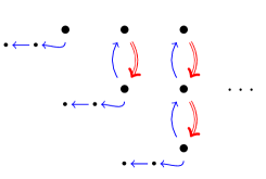
(a) Expansions: double arrows represent the rela-
tion $R$, single arrows—the relation $S$.

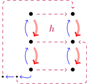
(b) A homomorphism ( dashed arrows) from an expansion of length 3 to its own prefix of length 2.

Figure 2: Illustrations for the query $\{\eqref{rule:pure-datalog-recursive},\eqref{rule:pure-datalog-initial-bounded}\},G)$ of Example 4.1.

The authors of [14] construct finite state automata for languages $\textit{expand}(\pi,G)$ and $\textit{notaccept}(\pi,G)$, the complement of $\textit{accept}(\pi,G)$, and use them to check their criterion in polynomial space. Our goal is to generalise this technique to the temporalised case. However, we can not use finite automata to work directly with sequences of rule bodies, since the language $\textit{accept}(\pi,G)$, in the presence of time, may be non-regular, as demonstrated by the following example.

Example 4.2.

Consider a program

$$G(X)\leftarrow R(X,Y)\wedge G(Y) G(X)\leftarrow A(X)\wedge{\raisebox{1.07639pt}{\text{\scriptsize{$\bigcirc$}}}}G(X)$$

$$G(X)\leftarrow P(X)\wedge{\raisebox{1.07639pt}{\text{\scriptsize{$\bigcirc$}}}^{-}}G(X) G(X)\leftarrow P(X)\wedge R(Y,X).$$

Denote its rule bodies $B_{1}(X,Y)=R(X,Y)\wedge G(Y)$, $B_{2}(X)=A(X)\wedge{\raisebox{1.07639pt}{\text{\scriptsize{$\bigcirc$}}}}G(X)$, and $B_{3}(X)=P(X)\wedge{\raisebox{1.07639pt}{\text{\scriptsize{$\bigcirc$}}}^{-}}G(X)$, and the composition $w=B_{1}B_{2}B_{2}B_{3}B_{3}B_{3}$. The composition $w$ is in $\textit{accept}(\pi,G)$, and the corresponding database $\mathcal{D}_{w}$ is given in Figure 3(a). In general, a composition of the form $B_{1}B_{2}^{n}B_{3}^{k}$ is in $\textit{accept}(\pi,G)$ if and only if $n<k$, which, by a simple application of the pumping lemma, is a non-regular language.

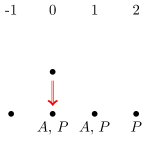
(a) The temporal database $\mathcal{D}_{w}$ for $w=B_{1}B_{2}B_{2}B_{3}B_{3}B_{3}$ of Example 4.2.

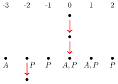
(b) The temporal database $\mathcal{D}_{w}$ for $w=B_{1}^{2}B_{2}^{2}B_{3}^{5}B_{2}B_{1}$ of Example 4.3.

Figure 3: Expansions of $\textsl{datalog}_{m}^{\,\smash{\raisebox{0.0pt}{$\scriptscriptstyle\bigcirc$}}}$ queries.

To overcome this, we introduce a larger alphabet and define more general versions of the languages $\textit{expand}(\pi,G)$ and $\textit{accept}(\pi,G)$ to regain their regularity. Recall that every composition $w$ of rule bodies gives rise to a temporal database $\mathcal{D}_{w}$. Instead of working with $w$, we use an exponentially larger alphabet $\Omega=2^{\Gamma_{\pi}^{r}\cup\Gamma_{\pi}^{i}\cup\{\bot,\top\}}$ to describe $\mathcal{D}_{w}$ as a word and define analogues of $\textit{expand}(\pi,G)$ and $\textit{accept}(\pi,G)$ over that alphabet. Consider a recursive rule

$$D(X)\leftarrow{\raisebox{1.07639pt}{\text{\scriptsize{$\bigcirc$}}}}^{k_{1}}R_{1}(\overline{U}_{1})\wedge\dots\wedge{\raisebox{1.07639pt}{\text{\scriptsize{$\bigcirc$}}}}^{k_{s}}R_{s}(\overline{U}_{s})\wedge{\raisebox{1.07639pt}{\text{\scriptsize{$\bigcirc$}}}}^{k}E(Y),$$ (29)

where $E(Y)$ is the unique IDB atom in the rule body and $k_{i},k\in\mathbb{Z}$. We call such a rule horizontal if $X=Y$ and vertical otherwise. In a composition $w\in(\Gamma^{r}_{\pi})^{*}\cup(\Gamma^{r}_{\pi})^{*}\Gamma_{\pi}^{i}$, a vertical (horizontal) segment is a maximal subword that consists of vertical (respectively, horizontal) rule bodies. For every composition $w$ we define the description $[w]\in\Omega^{*}$ of the respective database $\mathcal{D}_{w}$ as follows. Let $w=x_{1}y_{1}x_{2}y_{2}\dots x_{n}y_{n}$, where $x_{i}$ are vertical segments and $y_{i}$ are horizontal segments, with $x_{1}$ and $y_{n}$ possibly empty. For each $x_{i}=B_{1}\dots B_{n}$ we set $[x_{i}]$ to be the sequence $\{B_{1}\}\dots\{B_{n}\}$ of singleton sets, each of which contains a vertical rule body. For each $y_{i}=B_{1}\dots B_{n}$, we construct $[y_{i}]$ in $n$ steps, as follows. Recall that $B_{j}$, $1\leqslant j<n$, has the form $A_{j}(X,\mathbf{U})\wedge{\raisebox{1.07639pt}{\text{\scriptsize{$\bigcirc$}}}}^{m_{j}}D(X)$, where $D(X)$ is the unique IDB atom in $B_{j}$. Let $\ell_{1}=0$ and $\ell_{j}=\sum_{i=1}^{j-1}m_{i}$ for $j\leq n$. Intuitively, $\ell_{j}$ is the moment of time where the body $B_{j}$ lands in the composition $B_{1}\circ\dots\circ B_{n}$. Let $\ell^{\prime}_{1},\dots,\ell^{\prime}_{s}$ be the ordering of the the numbers in the set $\{\ell_{j}\}_{j=1}^{n}$ in the increasing order. We set, $\alpha_{\ell^{\prime}_{k}}$ to be $\{B_{j}\mid\ell_{j}=\ell^{\prime}_{k}\}$ for $\ell^{\prime}_{k}\in\{\ell_{1},\ell_{n}\}$; $\{B_{j}\mid\ell_{j}=\ell_{1}\}\cup\{\bot\}$ for $\ell^{\prime}_{k}=\ell_{1}\neq\ell_{n}$; $\{B_{j}\mid\ell_{j}=\ell_{n}\}\cup\{\top\}$ for $\ell^{\prime}_{k}=\ell_{n}\neq\ell_{1}$; and $\{B_{j}\mid\ell_{j}=\ell_{1}\}\cup\{\top,\bot\}$ for $\ell^{\prime}_{k}=\ell_{1}=\ell_{n}$. Additionally, we set $\alpha_{k}=\emptyset$ for $k\in[\ell^{\prime}_{1},\ell^{\prime}_{s}]\setminus\{\ell^{\prime}_{1},\dots,\ell^{\prime}_{s}\}$. Now we take $[y_{i}]=\alpha$.

Finally, $[w]=[x_{1}][y_{1}]\dots[x_{n}][y_{n}]$. We use the symbol $\Lambda$ to refer to letters of $[w]$. We call letters of the form $\{B\}$, where $B$ is a vertical rule body, vertical letters, and the rest—horizontal letters. Consequently, we can speak of vertical and horizontal segments of $[w]$, meaning maximal segments composed of vertical (respectively, horizontal) letters only.

Intuitively, $[w]$ describes $\mathcal{D}_{w}$, which can be seen as composed of $\mathcal{D}_{x_{1}},\mathcal{D}_{y_{1}},\dots,\mathcal{D}_{x_{n}},\mathcal{D}_{y_{n}}$, described by $[x_{1}],[y_{1}],\dots,[x_{n}],[y_{n}]$, respectively. The symbol $\bot$, representing a vertical line meeting a horizontal one, marks the point in time where $\mathcal{D}_{x_{i}}$ is connected to $\mathcal{D}_{y_{i}}$, while the symbol $\top$, analogously, shows where $\mathcal{D}_{y_{i}}$ is connected to $\mathcal{D}_{x_{i+1}}$.

Example 4.3.

Recall the rule bodies of Example 4.2 and consider the composition $w=B_{1}^{2}B_{2}^{2}B_{3}^{5}B_{2}B_{1}$. The corresponding $\mathcal{D}_{w}$ is depicted in Figure 3(b). Then $x_{1}=B_{1}^{2}$, $y_{1}=B_{2}^{2}B_{3}^{5}B_{2}$, $x_{2}=B_{1}$ and $y_{2}$ is empty. Thus, $[w]$ is equal to

$$\{B_{1}\}\{B_{1}\}\{B_{2}\}\{\top,B_{3}\}\{B_{3}\}\{\bot,B_{2},B_{3}\}\{B_{2},B_{3}\}\{B_{3}\}\{B_{1}\}$$ (30)

Not every word over $\Omega$ correctly describes a temporal database. This motivates the following definition: $\alpha\in\Omega^{*}$ is correct if (i) every symbol $\Lambda$ is either a singleton (standing for a vertical rule body) or a set of horizontal rule bodies, with a possible addition of $\bot,\top$, and (ii) every horizontal segment of $\alpha$ preceded by a vertical segment contains exactly one $\bot$, and every horizontal segment followed by a vertical one—exactly one $\top$. A correct word $\alpha\in\Omega^{*}$ describes a temporal database $\mathcal{D}_{\alpha}$ similarly to how $[w]$ describes $\mathcal{D}_{w}$. Formally, break $\alpha$ into vertical/horizontal segments $\chi_{1}\upsilon_{1}\dots\chi_{n}\upsilon_{n}$. For a vertical segment $\chi_{i}=\{B_{1}\}\dots\{B_{n}\}$, set $Q_{\chi_{i}}=B_{1}\circ\dots\circ B_{n}$. For a horizontal segment $\upsilon_{i}=\Lambda_{1}\dots\Lambda_{s}$, let $\Lambda_{j_{\bot}}$ be the one containing $\bot$ and $\Lambda_{j_{\top}}$—containing $\top$. Then $Q_{\upsilon_{i}}$ is the conjunction of rule bodies from $\upsilon_{i}$, where each $B\in\Lambda_{j}$ is prefixed by ${\raisebox{1.07639pt}{\text{\scriptsize{$\bigcirc$}}}}^{j-j_{\bot}}$, plus, if $i\neq n$, an IDB atom ${\raisebox{1.07639pt}{\text{\scriptsize{$\bigcirc$}}}}^{j_{\top}-j_{\bot}}D(X)$. Finally, set $\mathcal{D}_{\alpha}=\mathcal{D}_{Q_{\alpha}}$ for $Q_{\alpha}=Q_{\chi_{1}}\circ Q_{\upsilon_{1}}\circ\dots\circ Q_{\chi_{n}}\circ Q_{\upsilon_{n}}$. This $Q_{\alpha}$ will be also useful further.

We are now ready to define languages over $\Omega$ that will be useful to study the data complexity of our queries. Let ${\textit{Accept}}(\pi,G)$ be the language of correct words $\alpha$ such that $\mathcal{D}_{\alpha},\pi,0\models G(X)$, with $X\in\Delta_{\mathcal{D}_{\alpha}}$, and $\textit{NotAccept}(\pi,G)$ be its complement. We need to define the language of expansions over the alphabet $\Omega$ that we will use together with the language $\textit{NotAccept}(\pi,G)$ to formulate a criterion for L-hardness similar to the one of [14]. It would be natural to take the language of expansions as $\{[w]\mid w\in\textit{expand}(\pi,G)\}$. However, it is harder to define an automaton recognising such a language than it is for the language of $[w]$s as above where each horizontal letter $[w]_{i}$ may be extended (as a set) with arbitrary “redundant” rule bodies, and each horizontal segment may be extended, from the left and right, by “redundant” horizontal letters. For example, we will include into the language of expansions the word $\{B_{1}\}\{B_{1}\}\{B_{3}\}\{B_{2},B_{3}\}\{\top,B_{3}\}\{B_{2},B_{3}\}\{\bot,B_{2},B_{3}\}\{B_{2},B_{3}\}\{B_{3}\}\{B_{1}\}$ alongside (30). It turns out that the latter language works for our required criteria as good as the former one. Formally, if $\alpha,\beta\in\Omega^{*}$, we write $\alpha\preccurlyeq\beta$ if $\alpha=x_{1}y_{1}\dots x_{n}y_{n}$ and $\beta=x_{1}y^{\prime}_{1}\dots x_{n}y^{\prime}_{n}$, where $x_{i}$ are vertical segments and $y_{i},y^{\prime}_{i}$ are horizontal segments, and if $y_{i}=a_{1}\dots a_{m}$, $y^{\prime}_{i}=b_{1}\dots b_{s}$, then there is $k\geqslant 0$ such that $m+k\leqslant s$ and $a_{j}\subseteq b_{j+k}$, $1\leqslant j\leqslant m$. We define $\textit{Expand}_{\preccurlyeq}(\pi,G)$ to be the set of correct words $\alpha\in\Omega^{*}$ such that $[w]\preccurlyeq\alpha$ for some $w\in\textit{expand}(\pi,G)$.

It is important for our purposes that these languages are regular. For $\textit{Expand}_{\preccurlyeq}(\pi,G)$, the rules of the program $\pi$ may be naturally seen as transition rules of a two-way automaton whose states are the IDBs of $\pi$ (plus a final state). The initial state is the one associated with $G$, and the final state is reached by an application of an initialisation rule.

Lemma 4.4.

For any $\textsl{datalog}_{\it lm}^{\,\smash{\raisebox{0.0pt}{$\scriptscriptstyle\bigcirc$}}}$-query $(\pi,G)$, the language $\textit{Expand}_{\preccurlyeq}(\pi,G)$ is regular.

The case of $\textit{NotAccept}(\pi,G)$ is more involved. Generalising from [14], for an automaton to recognise if $\alpha\in\textit{NotAccept}(\pi,G)$ it suffices to guess (by nondeterminism) an enrichment $\mathcal{E}$ of $\mathcal{D}_{\alpha}$, and check that $\mathcal{E}$ is a model of $\pi$ and that $\mathcal{E}$ does not contain the atom $G(X)$. Moreover, since $\pi$ is connected, for $\mathcal{E}$ to be a model it is enough that every piece of $E$ of radius $|\pi|$, in terms of Gaifman graph, satisfies all the rules. The idea is to precompute the answer for each such piece and encode them in the state-space of the automaton. The problem, specific to the temporalised case, is that enrichments are infinite in the temporal dimension. To resolve this, we observe that there are still finitely many EDB atoms in $\mathcal{E}$. Since, once again, $\pi$ is connected, to check that rules with EDBs are satisfied it is enough to consider only those pieces of $\mathcal{E}$ that contain an EDB atom. For the rest of the rules, it suffices to check if such a finite piece can be extended into an infinitely in time to give a model of $\pi$. The rules without EDBs can be seen as plain L​TL rules, so we can employ satisfiability checking for L​TL to perform this check.

Lemma 4.5.

For any $\textsl{datalog}_{\it lm}^{\,\smash{\raisebox{0.0pt}{$\scriptscriptstyle\bigcirc$}}}$-query $(\pi,G)$, the language $\textit{NotAccept}(\pi,G)$ is regular.

Corollary 4.6.

For any $\textsl{datalog}_{\it lm}^{\,\smash{\raisebox{0.0pt}{$\scriptscriptstyle\bigcirc$}}}$-query $(\pi,G)$, the language ${\textit{Accept}}(\pi,G)$ is regular.

5 Decidability for Connected Linear Queries with $\bigcirc$

We use the automata introduced in the previous section to prove a positive result.

Theorem 5.1.

(i) Every connected $\textsl{datalog}_{\it lm}^{\,\smash{\raisebox{0.0pt}{$\scriptscriptstyle\bigcirc$}}}$ query is either in $\textsc{AC}^{0}$, or in ${\textsc{ACC}^{0}}\setminus{\textsc{AC}^{0}}$, or $\textsc{NC}^{1}$-complete, or L-hard. (ii) It is PSpace-complete to check whether such a query is L-hard; whether it belongs to $\textsc{AC}^{0}$, ${\textsc{ACC}^{0}}$, or is $\textsc{NC}^{1}$-complete can be decided in ExpSpace.

We first deal with (i). Intuitively, L-hardness is a consequence of the growth of query expansions in the relational domain. If this growth is limited, the query essentially defines a certain temporal property, which can be checked in $\textsc{NC}^{1}$. Formally, given a word $\alpha\in\Omega^{*}$, we define the $0pt{\alpha}$ as the number of vertical letters in $\alpha$. Then, we call a query vertically unbounded if for every $k$ there is a word $\alpha\in\textit{Accept}(\pi,G)$, $0pt{\alpha}>k$, such that every prefix of $\alpha$ of height $k$ is in $\textit{NotAccept}(\pi,G)$. Otherwise, the query is called vertically bounded.

Vertically unbounded queries can be shown to be L-hard by a direct reduction from the undirected reachability problem. Namely, take the deterministic automata for $\textit{NotAccept}(\pi,G)$ and ${\textit{Accept}}(\pi,G)$, supplied by Lemma 4.5 and Corollary 4.6, and apply the pumping lemma to obtain words $\xi,\upsilon,\zeta,\gamma$ such that $0pt{\upsilon}>0$, $\xi\upsilon^{i}\zeta\in\textit{NotAccept}(\pi,G)$ and $\xi\upsilon^{i}\zeta\gamma\in{\textit{Accept}}(\pi,G)$, for all $i\geqslant 0$. Then, given a graph $\mathcal{G}$ and two nodes $s,t$, use copies of $\mathcal{D}_{\upsilon}$ to simulate the edges of $\mathcal{G}$, and attach $\mathcal{D}_{\xi}$ to $s$ and $\mathcal{D}_{\zeta\gamma}$ to $t$. Thus, you will obtain a temporal database $\mathcal{D}_{\mathcal{G}}$, where $\mathcal{D}_{\mathcal{G}},\pi,0\models G(s)$ if and only if there is a path from $s$ to $t$.

Lemma 5.2.

If a query is vertically unbounded, then it is L-hard.

Observe that $\mathcal{D},\pi,\ell\models G(d)$ whenever $\mathcal{D},\ell\models Q_{\alpha}(d)$ for some $\alpha\in\textit{Accept}(\pi,G)$. If $\mathcal{D},\ell\models Q_{\alpha}(d)$, then $x_{1},y_{1},\dots,y_{n},x_{n}$, the vertical and horizontal segments of $\alpha$, appear in $\mathcal{D}$, starting from $d$ at time $\ell$. Expand $y_{i}$ to $y^{\prime}_{i}$, the $\preccurlyeq$-maximal horizontal segment fitting in $\mathcal{D}$, and let $\beta=x_{1}y^{\prime}_{1}\dots x_{n}y^{\prime}_{n}$. Then $\beta\in\textit{Accept}(\pi,G)$ and $\mathcal{D},\ell\models Q_{\beta}(d)$. Thus, to check $\mathcal{D},\pi,\ell\models G(d)$, it suffices to find vertical segments of some $\alpha\in\textit{Accept}(\pi,G)$, taking $\preccurlyeq$-maximal horizontal segments, and check that $\beta\in\textit{Accept}(\pi,G)$. If $(\pi,G)$ is vertically bounded, there are finitely many vertical segments of interest. Finding vertical segments, as well as extracting $\preccurlyeq$-maximal horizontal ones, can be done by an $\textsc{AC}^{0}$ circuit.

Lemma 5.3.

If $(\pi,G)$ is vertically bounded, then the data complexity of $(\pi,G)$ coincides with that of checking membership in ${\textit{Accept}}(\pi,G)$, modulo reductions computable in $\textsc{AC}^{0}$.

Recall that ${\textit{Accept}}(\pi,G)$ is a regular language, so checking membership in it is either in $\textsc{AC}^{0}$, or ${\textsc{ACC}^{0}}\setminus{\textsc{AC}^{0}}$, or $\textsc{NC}^{1}$-complete [42]. This settles the part (i) of Theorem 5.1: a query is either vertically unbounded and thus L-hard, or vertically bounded and thus belongs to one of the three classes mentioned above.

It remains to address the part (ii) of Theorem 5.1. By a careful analysis of the proof of Lemma 4.5 one can show that $\textit{NotAccept}(\pi,G)$ is recognised by a nondeterministic automaton of size $2^{{\mathrm{poly}\left(|\pi|\right)}}$. Further, checking whether its language belongs to ${\textsc{AC}^{0}}$, ${\textsc{ACC}^{0}}\setminus{\textsc{AC}^{0}}$, or is $\textsc{NC}^{1}$-complete, can be done via the polynomial-space procedure developed in [30]. Thus, given a vertically bounded query, its data complexity can be established in exponential space.

For the vertical boundedness itself, note that substituting $\textit{Accept}(\pi,G)$ with $\textit{Expand}_{\preccurlyeq}(\pi,G)$ in the respective definition preserves all the results proven so far. For $\textit{Expand}_{\preccurlyeq}(\pi,G)$, we can get from Lemma 4.4 an exponential-size one-way automaton. Checking that the query is vertically unbounded can be done in nondeterministic space logarithmic in the size of the automata for $\textit{Expand}_{\preccurlyeq}(\pi,G)$ and $\textit{NotAccept}(\pi,G)$, as it boils down to checking reachability in their Cartesian product.

Lemma 5.4.

Checking if a connected $\textsl{datalog}_{\it lm}^{\,\smash{\raisebox{0.0pt}{$\scriptscriptstyle\bigcirc$}}}$ query is vertically bounded is in PSpace.

For the lower bound, we show that checking boundedness is already PSpace-hard for connected linear monadic queries in plain datalog. In fact, PSpace-hardness was proved in [14] for program boundedness of disconnected programs. A program $\pi$ is called bounded if $(\pi,G)$ is bounded for every IDB $G$ in $\pi$. We were able to regain the connectedness of $\pi$ by focusing on query boundedness (also called predicate boundedness) instead. The idea combines that of [14] with that of Section 3: define an IDB $F$ that slides along a computation, this time of a space-bounded Turing machine, looking for an erroneous transition.

Lemma 5.5.

Deciding boundedness of connected linear monadic queries in plain datalog is PSpace-hard.

Lemmas 5.2 and 5.3 bring us to an interesting consideration: to understand the data complexity of a given query one should analyse its behaviour in the relational domain separately from that in the temporal domain. This can be given a precise sense as follows.

Proposition 5.6.

For every connected $\textsl{datalog}_{\it lm}^{\,\smash{\raisebox{0.0pt}{$\scriptscriptstyle\bigcirc$}}}$ query $(\pi,G)$ there exist a plain datalog query $(\pi_{d},G)$ and a plain L​TL query $(\pi_{t},G)$, such that:

1. $(\pi,G)$ is vertically bounded if and only if $(\pi_{d},G)$ is bounded;

2. if $(\pi,G)$ is vertically bounded then its data complexity coincides with that of $(\pi_{t},G)$.

This highlights the ‘weak’ kind of interaction between the two domains provided by the operators $\bigcirc$ and $\raisebox{1.07639pt}{\text{\scriptsize{$\bigcirc$}}}^{-}$. Given the undecidability results of Section 3, no such or similar decomposition is possible for queries with $\Diamond$.

Technically, both $\pi_{d}$ and $\pi_{t}$ are obtained by simulating the deterministic automaton $\mathcal{A}_{(\pi,G)}$ for the language ${\textit{Accept}}(\pi,G)$ provided by Corollary 4.6. In both programs, the IDBs correspond to the states of $\mathcal{A}_{(\pi,G)}$ and EDBs to the letters of $\Omega$. For $\pi_{t}$ these EDBs are unary and all the rules are horizontal, so that the expansions unwind fully in the temporal domain. In the case of $\pi_{d}$, the EDBs are binary and every vertical transition of $\mathcal{A}_{(\pi,G)}$ is a step by a binary relation, while the horizontal transitions are skipped (thus, vertical boundedness becomes just boundedness). In both programs, initialisation rules correspond to $\mathcal{A}_{(\pi,G)}$ reaching an accepting state.

We conclude this section with a consideration on disconnected queries. In [14], deciding boundedness is based on the fact that $\textit{accept}(\pi,G)$ remains regular even when $\pi$ has disconnected rules. This is not the case for $\textsl{datalog}_{\it lm}^{\,\smash{\raisebox{0.0pt}{$\scriptscriptstyle\bigcirc$}}}$, as can be seen from the following example.

Example 5.7.

Consider the program $\pi$ of four rules:

$$G(X)\leftarrow A(X)\wedge{\raisebox{1.07639pt}{\text{\scriptsize{$\bigcirc$}}}}D(X) D(X)\leftarrow{\raisebox{1.07639pt}{\text{\scriptsize{$\bigcirc$}}}}D(X)$$

$$D(X)\leftarrow R(X,Y)\wedge{\raisebox{1.07639pt}{\text{\scriptsize{$\bigcirc$}}}^{-}}B(Y)\wedge{\raisebox{1.07639pt}{\text{\scriptsize{$\bigcirc$}}}^{-}}D(Y) D(X)\leftarrow A(Y)\wedge B(X)$$

Let $B_{1}=A(X)\wedge{\raisebox{1.07639pt}{\text{\scriptsize{$\bigcirc$}}}}D(X)$, $B_{2}={\raisebox{1.07639pt}{\text{\scriptsize{$\bigcirc$}}}}D(X)$, and $B_{3}=R(X,Y)\wedge{\raisebox{1.07639pt}{\text{\scriptsize{$\bigcirc$}}}^{-}}B(Y)\wedge{\raisebox{1.07639pt}{\text{\scriptsize{$\bigcirc$}}}^{-}}D(Y)$. Then $B_{1}B_{2}^{n}B_{3}^{m}\in\textit{accept}(\pi,G)$, and, consequently, $\{\bot,B_{1}\}\{B_{2}\}^{n}\{\top\}\{B_{3}\}^{m}\in\textit{Accept}(\pi,G)$, whenever $m>n\geqslant 1$. This property is not recognisable by any finite state automaton. For more general classes of automata suitable to recognise $\textit{accept}(\pi,G)$ or $\textit{Accept}(\pi,G)$ in the disconnected setting, the properties that are to be checked along the lines of [14], such as language emptiness or finiteness, become undecidable. Therefore, disconnected queries possibly require a different approach for analysing the data complexity.

6 Conclusions and Future Work

We have started investigating the complexity of determining the data complexity of answering monadic datalog queries with temporal operators. For linear connected queries with operators $\bigcirc$/$\raisebox{1.07639pt}{\text{\scriptsize{$\bigcirc$}}}^{-}$, we have generalised the automata-theoretic technique of [14], developed originally for plain datalog, to establish an ${\textsc{AC}^{0}}/{\textsc{ACC}^{0}}/{\textsc{NC}^{1}}/\textsc{L}/\textsc{NL}$ classification of temporal query answering and proved that deciding L-hardness of a given query is PSpace-complete, while checking its membership in $\textsc{AC}^{0}$ or $\textsc{ACC}^{0}$ can be done in ExpSpace. As a minor side product, we have established PSpace-hardness of deciding boundedness of atemporal connected linear monadic datalog queries. Rather surprisingly and in sharp contrast to the $\bigcirc$/$\raisebox{1.07639pt}{\text{\scriptsize{$\bigcirc$}}}^{-}$ case, it turns out that checking (non-trivial) membership of queries with operators $\Diamond$/$\raisebox{0.43057pt}{\text{\small{$\Diamond$}}}\!^{-}$ in the above complexity classes is undecidable. The results of this paper lead to a plethora of natural and intriguing open questions. Some of them are briefly discussed below.

1. What happens if we disallow applications of $\raisebox{0.43057pt}{\text{\small{$\Diamond$}}}/\raisebox{0.43057pt}{\text{\small{$\Diamond$}}}\!^{-}$ to binary EDB predicates in $\textsl{datalog}_{\it lm}^{\,\smash{\raisebox{-1.0pt}{$\diamond$}}}$-queries? We conjecture that this restriction makes checking membership in the above complexity classes decidable. In fact, this conjecture follows from a positive answer to the next question.

2. Can our decidability results for $\textsl{datalog}_{\it lm}^{\,\smash{\raisebox{0.0pt}{$\scriptscriptstyle\bigcirc$}}}$ be lifted to $\textsl{datalog}_{m}^{\,\smash{\raisebox{0.0pt}{$\scriptscriptstyle\bigcirc$}}}$-queries? Dropping the linearity restriction in the atemporal case results in the extra data complexity class, P, and the higher complexity, 2ExpTime-completeness, of deciding boundedness. The upper bound was obtained using tree automata in [14], and we believe that this approach can be generalised to connected $\textsl{datalog}_{m}^{\,\smash{\raisebox{0.0pt}{$\scriptscriptstyle\bigcirc$}}}$-queries in a way similar to what we have done above.

3. On the other hand, dropping the connectedness restriction might turn out to be trickier, if at all possible, as shown by Example 5.7. Finding a new automata-theoretic characterisation for disconnected $\textsl{datalog}_{\it lm}^{\,\smash{\raisebox{0.0pt}{$\scriptscriptstyle\bigcirc$}}}$-queries remains a challenging open problem.

4. A decisive step in understanding the data complexity of answering queries mediated by a description logic ontology and monadic disjunctive datalog queries was made in [8, 17] by establishing a close connection with constraint satisfaction problems (CSPs). In our case, quantified CSPs (see, e.g., [49]) seem to be more appropriate. Connecting the two areas might be beneficial to both of them.

5. In the context of streaming data, it would be interesting to investigate the data complexity classes and the complexity of recognising them for datalogMTL-queries [9, 37, 46].

Appendix A Proofs for Section 2

See 2.1

Proof A.1.

Let $\Sigma$ be a database schema and $\mathcal{D}$—a temporal database over $\Sigma$. Let $\Sigma^{\prime}=\{R^{m+1}|R^{m}\in\Sigma\}$, where the superscript $m$ denotes the arity of the relation symbol $R$. Then $\mathfrak{S}_{\mathcal{D}}$ is a two-sorted first-order structure over the signature $\Sigma^{\prime}\cup\{<\}$ with the domain $\Delta_{\mathcal{D}}\cup\mathrm{tem}(\mathcal{D})$, and such that $R(\bar{d},\ell)$ is true in $\mathfrak{S}_{\mathcal{D}}$ if and only if $\bar{d}\in\Delta_{\mathcal{D}}^{m},\ell\in\mathrm{tem}(\mathcal{D})$ and $\mathcal{D},\ell\models R(\bar{d})$. Moreover, $(\ell<\ell^{\prime})$ is true in $\mathfrak{S}_{\mathcal{D}}$ whenever $\ell,\ell^{\prime}\in\mathrm{tem}(\mathcal{D})$ and $\ell<\ell^{\prime}$ in $\mathbb{Z}$. The truth relation $\models$ for two-sorted first-order formulas over $\mathfrak{S}_{\mathcal{D}}$ are defined in the expected way (see [4] for details).

We show that there exists an $\textup{FO}(<)$-formula $\psi_{Q}(\overline{X},t)$ such that for any $\mathcal{D}$, any $\bar{d}\in\Delta_{\mathcal{D}}^{|\overline{X}|}$, and any $\ell\in\mathrm{tem}(\mathcal{D})$, $\mathcal{D},\ell\models Q(\bar{d})$ if and only if $\psi_{Q}(\bar{d},\ell)$ is true in $\mathfrak{S}_{\mathcal{D}}$. For simplicity, we slightly abuse the notation and write $\mathcal{D}\models\psi(\bar{d},\ell)$. We first prove two auxiliary lemmas.

Lemma A.2.

If $\varphi(\overline{Z})$ is defined by (5) and has $N$ temporal operators, then for any $\mathcal{D}$ with $\mathrm{tem}(\mathcal{D})=[l,r]$ and any $\bar{d}\in\Delta_{\mathcal{D}}^{|\overline{Z}|}$:

$$\mathcal{D},r+N+1\models\varphi(\bar{d})\iff\mathcal{D},\ell\models\varphi(\bar{d}),\text{ for all $\ell>r+N$}$$ (31)

$$\mathcal{D},l-N-1\models\varphi(\bar{d})\iff\mathcal{D},\ell\models\varphi(\bar{d}),\text{ for all $\ell<l-N$}$$ (32)

Proof A.3.

The proof is by induction. For $N=0$, $\varphi$ is a conjunction of atoms. Clearly, $\mathcal{D},\ell\not\models\varphi(\bar{d})$ for any $\ell\notin[l,r]$. We justify the induction step for (31), while the case of (32) is analogous. We do another induction on the structure of the formula. The case $\varphi=R(Z_{1},\dots,Z_{m})$ is trivial. In the case $\varphi=\varphi_{1}\wedge\varphi_{2}$ by the induction hypothesis on $N$ everything works. For the temporal operators, we consider the most interesting case of $\varphi=\raisebox{0.43057pt}{\text{\small{$\Diamond$}}}\!^{-}\varphi_{1}$, while the other cases can be proved by a simple application of the induction hypothesis and are left to the reader. Let $\varphi=\raisebox{0.43057pt}{\text{\small{$\Diamond$}}}\!^{-}\varphi_{1}$. If $\mathcal{D},\ell\not\models\raisebox{0.43057pt}{\text{\small{$\Diamond$}}}\!^{-}\varphi_{1}(\bar{d})$ for all $\ell>r+N$, we are done. Otherwise, let $\ell_{0}>r+N$ be the least timestamp such that $\mathcal{D},\ell\models\raisebox{0.43057pt}{\text{\small{$\Diamond$}}}\!^{-}\varphi_{1}(\bar{d})$. By the choice of $\ell_{0}$, $\mathcal{D},\ell_{0}-1\models\varphi_{1}(\bar{d})$, where $\ell_{0}-1\geqslant r+N$. By the induction hypothesis, $\mathcal{D},r+N\models\varphi_{1}(\bar{d})$, thus $\mathcal{D},r+N\models\varphi_{1}(\bar{d})$, and therefore $\mathcal{D},\ell\models\raisebox{0.43057pt}{\text{\small{$\Diamond$}}}\!^{-}\varphi_{1}(\bar{d})$ for $\ell>r+N$.

Lemma A.4.

Let $\varphi(\overline{Z})$ be defined by (5). For any subformula $\varkappa(\overline{Z})$ of $\varphi$, there exist formulas $\psi_{\varkappa}(\overline{Z},t)$ and $\psi_{\varkappa}^{i}(\overline{Z})$ for $i\in[-N-1,\dots,-1]\cup[1,\dots,N+1]$, such that for any $\mathcal{D}$ with $\mathrm{tem}(\mathcal{D})=[l,r]$ and any objects $\bar{d}\in\Delta_{\mathcal{D}}^{|\overline{Z}|}$ we have:

$$\mathcal{D},\ell\models\varkappa(\bar{d})\iff\mathcal{D}\models\psi_{\varkappa}(\bar{d},\ell),\text{ for }l\leqslant\ell\leqslant r$$ (33)

$$\mathcal{D},(r+i)\models\varkappa(\bar{d})\iff\mathcal{D}\models\psi_{\varkappa}^{i}(\bar{d}),\text{ for }1\leqslant i\leqslant N+1$$ (34)

$$\mathcal{D},(l+i)\models\varkappa(\bar{d})\iff\mathcal{D}\models\psi_{\varkappa}^{i}(\bar{d}),\text{ for }-N-1\leqslant i\leqslant 1$$ (35)

Proof A.5.

The proof is, once again, by induction. For the base case, we set $\psi_{R}(\overline{Z},t)=R(\overline{Z},t)$ and $\psi_{R}^{i}(\overline{Z})=\bot$. For an induction step, let $\min$ be defined by $\forall t(\min\leqslant t)$ and $\max$ by $\forall t(t\leqslant\max)$, and the predicate $t^{\prime}=t+1$ by $(t<t^{\prime})\wedge\forall\tau.[(\tau<t)\wedge(\tau<t^{\prime})]\vee[(t<\tau)\wedge(t^{\prime}<\tau)]$. Then we define:

$$\psi_{\varkappa_{1}\wedge\varkappa_{2}}=\psi_{\varkappa_{1}}\wedge\psi_{\varkappa_{2}}$$ (36)

$$\psi^{i}_{\varkappa_{1}\wedge\varkappa_{2}}=\psi^{i}_{\varkappa_{1}}\wedge\psi^{i}_{\varkappa_{2}},\text{ for all }i$$ (37)

$$\psi_{{\raisebox{0.75346pt}{\text{\scriptsize{$\bigcirc$}}}}\varkappa}^{-1}(\overline{Z})=\psi_{\varkappa}(\overline{Z},\min)$$ (38)

$$\psi_{{\raisebox{0.75346pt}{\text{\scriptsize{$\bigcirc$}}}}\varkappa}^{N+1}(\overline{Z})=\psi^{N+1}_{\varkappa}(\overline{Z})$$ (39)

$$\psi_{{\raisebox{0.75346pt}{\text{\scriptsize{$\bigcirc$}}}}\varkappa}^{i}(\overline{Z})=\psi_{\varkappa}^{i+1}(\overline{Z}),\text{ for all other }i$$ (40)

$$\psi_{{\raisebox{0.75346pt}{\text{\scriptsize{$\bigcirc$}}}}\varkappa}(\overline{Z},t)=\exists t^{\prime}[(t^{\prime}=t+1)\land\psi_{\varkappa}(\overline{Z},t^{\prime})]\lor((t=\max)\land\psi_{\varkappa}^{1}(\overline{Z}))$$ (41)

$$\psi_{\raisebox{0.3014pt}{\text{\small{$\Diamond$}}}\varkappa}^{i}(\overline{Z})=\bigvee_{i<j\leqslant N+1}\psi^{j}_{\varkappa}(\overline{Z}),\text{ for }0<i<N+1$$ (42)

$$\psi_{\raisebox{0.3014pt}{\text{\small{$\Diamond$}}}\varkappa}^{i}(\overline{Z})=\bigvee_{i<j\leqslant N+1}\psi^{j}_{\varkappa}(\overline{Z})\wedge\exists t[(\min\leqslant t\leqslant\max)\wedge\psi_{\varkappa}(\overline{Z},t)],\text{ for }-N-1\leqslant i<0$$ (43)

$$\psi_{\raisebox{0.3014pt}{\text{\small{$\Diamond$}}}\varkappa}^{N+1}(\overline{Z})=\psi^{N+1}_{\varkappa}(\overline{Z})$$ (44)

$$\psi_{{\raisebox{0.75346pt}{\text{\scriptsize{$\bigcirc$}}}}\varkappa}(\overline{Z},t)=\exists t^{\prime}[(t<t^{\prime})\land\psi_{\varkappa}(\overline{Z},t^{\prime})]\lor\bigvee_{1\leqslant i\leqslant N+1}\psi^{i}_{\varkappa}(\overline{Z})$$ (45)

And analogously for $\raisebox{1.07639pt}{\text{\scriptsize{$\bigcirc$}}}^{-}$ and $\raisebox{0.43057pt}{\text{\small{$\Diamond$}}}\!^{-}$. The correctness of the induction step follows from the semantics of temporal operators and Lemma A.2.

Now, for $Q=\exists\overline{U}\varphi(\overline{X},\overline{U})$, we apply Lemma A.4 to $\varphi(\overline{X},\overline{U})$ and obtain $\psi_{\varkappa}(\overline{X},\overline{U},t)$. The required rewriting $\psi_{Q}(\overline{X},t)$ is then the formula $\exists\overline{U}\psi_{\varkappa}(\overline{X},\overline{U},t)$.

See 2.3

Proof A.6.

The lower bound for $\textsl{datalog}_{m}^{\,\scriptscriptstyle\bigcirc{\smash{\raisebox{-1.3pt}{$\diamond$}}}}$ follows from the analogous proof for temporal deductive databases [12, Appendix A], which uses only monadic IDBs and a ‘rigid’ relation $\textit{Next}(i,j)$ holding at every moment of time. To simulate the latter in $\textsl{datalog}_{m}^{\,\scriptscriptstyle\bigcirc{\smash{\raisebox{-1.3pt}{$\diamond$}}}}$, assert $\textit{Next}(i,j)$ at time $0$ and refer to it by $\raisebox{0.43057pt}{\text{\small{$\Diamond$}}}\!^{-}\textit{Next}(i,j)$ at later moments. The upper bound, for the full $\textsl{datalog}^{\,\scriptscriptstyle\bigcirc{\smash{\raisebox{-1.3pt}{$\diamond$}}}}$, is obtained by grounding rules of the program with the domain elements, obtaining a set of propositional L​TL formulas, converting the input database into a set of temporalised atoms (e.g. $R(\bar{d})\in D_{\ell}$ becomes ${\raisebox{1.07639pt}{\text{\scriptsize{$\bigcirc$}}}}^{\ell}R(\bar{d})$), and applying the polynomial-space satisfiability checking procedure for L​TL [31].

The rest of the proof in dedicated to the case of $\textsl{datalog}_{\it lm}^{\,\scriptscriptstyle\bigcirc{\smash{\raisebox{-1.3pt}{$\diamond$}}}}$. The lower bound follows from NL-hardness of query answering for plain linear datalog. To simplify the notation, we show the upper bound for the monadic queries only. The proof can be straightforwardly modified for the non-monadic case with $M_{\Pi,\mathcal{D}}$ in Lemma A.7 changing to $2(|\textit{IDB}(\pi)|(|\textup{dom}\mathcal{D}|)^{a})^{2}$, where $a$ is the maximal arity among $\textit{IDB}(\pi)$. For a program $\Pi$, a rule

$$C(X)\leftarrow B(X,Y,U_{1},\dots,U_{m})\ \wedge\ {\raisebox{1.07639pt}{\text{\scriptsize{$\bigcirc$}}}}^{k}D(Y),$$ (46)

($k\in\{-1,0,1\}$) with $C,D\in\textit{IDB}(\pi)$, data instance $\mathcal{D}$, $c,d\in\Delta_{\mathcal{D}}$ and $\ell\in\mathbb{Z}$, we write $C(c)\leftarrow^{B}_{\ell,k}D(d)$ if $\mathcal{D},\ell\models\exists U_{1},\dots,U_{m}(B(c,d,U_{1},\dots,U_{m}))$. We write $C(c)\leftarrow_{\ell,k}D(d)$ if there exists a rule (46) in $\Pi$ such that $C(c)\leftarrow_{\ell,k}^{B}D(d)$. Similarly, for an initialization rule

$$C(X)\leftarrow B(X,U_{1},\dots,U_{m}),$$ (47)

we write $C(c)\leftarrow^{B}_{\ell}$ if $\mathcal{D},\ell\models\exists U_{1},\dots,U_{m}(B(c,U_{1},\dots,U_{m}))$,
and we define $C(c)\leftarrow_{\ell}$ analogously. Firstly, we observe the following important monotonicity property:

$$C(c)\leftarrow_{\ell,k}D(d) \text{ iff }C(c)\leftarrow_{\ell^{\prime},k}D(d)$$

$$C(c)\leftarrow_{\ell} \text{ iff }C(c)\leftarrow_{\ell^{\prime}}$$ (48)

for any $c,d,C,D,k$ as above and any $\ell,\ell^{\prime}\in\mathbb{Z}$ such that either $\ell,\ell^{\prime}>\max\mathcal{D}+K_{\Pi}$ or $\ell,\ell^{\prime}<\min\mathcal{D}-K_{\Pi}$, where $K_{\Pi}$ is the maximal number of nested temporal operators in a rule body of $\Pi$.

We call

$$C_{0}(c_{0})\leftarrow_{\ell_{0},k_{0}}C_{1}(c_{1})\leftarrow_{\ell_{1},k_{1}}\dots\leftarrow_{\ell_{n-1},k_{n-1}}C_{n}(c_{n})$$ (49)

an entailment sequence from $C_{0}(c_{0})$ at $\ell_{0}$ to $C_{n}(c_{n})$ at $\ell_{n}$ in $\mathcal{D}$ if $C_{i}\in\textit{IDB}(\pi)$, $c_{i}\in\Delta_{\mathcal{D}}$, $\ell_{i}\in\mathbb{Z}$, $\ell_{i+1}=\ell_{i}+k_{i}$. An entailment sequence is called initialized if $C_{n}(c_{n})\leftarrow_{\ell_{n}}$. It should be clear that

$$\text{For all }\ell\in\mathbb{Z}\text{ and }g\in\textup{dom}(\mathcal{D}),\Pi,\mathcal{D},\ell\models G(g)\text{ iff }\\ \text{there exists some initialized entailment sequence from }G(g)\text{ at }\ell\text{ in }\mathcal{D}.$$

Our aim now is to show:

Lemma A.7.

If there exists an initialized entailment sequence from $C_{0}(c_{0})$ at $\ell_{0}\in[\min\mathcal{D},\max\mathcal{D}]$ in $\mathcal{D}$, then there exists an initialized entailment sequence $C_{0}(c_{0})\leftarrow_{\ell_{0},k_{0}}C_{1}(c_{1})\leftarrow_{\ell_{1},k_{1}}\dots\leftarrow_{\ell_{n-1},k_{n-1}}C_{n}(c_{n})$, with $\ell_{i}\in[\min\mathcal{D}-K_{\Pi}-M_{\Pi,\mathcal{D}},\max\mathcal{D}+K_{\Pi}+M_{\Pi,\mathcal{D}}]$, where $M_{\Pi,\mathcal{D}}=2(|\textit{IDB}(\pi)||\textup{dom}\mathcal{D}|)^{2}$.

Because each $\ell_{i}$ is at most quadratic in $|\mathcal{D}|$ it should be clear that there is an algorithm to check $\Pi,\mathcal{D},\ell\models G(g)$ that works in NL w.r.t. to $|\mathcal{D}|$. In the remainder, we prove the above Lemma.

Proof A.8.

Consider a sequence (49) in the assumption of the lemma and take the minimal $i$ such that:

• either $\ell_{i}=\max\mathcal{D}+K_{\Pi}+1$ and there exists $j>i$ with $\ell_{j}=\max\mathcal{D}+K_{\Pi}+2(|\textit{IDB}(\pi)||\textup{dom}\mathcal{D}|)^{2}+1$ and $\ell_{t}>\ell_{i}$ for all $i<t<j$,

• or $\ell_{i}=\min\mathcal{D}-K_{\Pi}-1$ and there exists $j>i$ with $\ell_{j}=\min\mathcal{D}-K_{\Pi}-2(|\textit{IDB}(\pi)||\textup{dom}\mathcal{D}|)^{2}-1$ and $\ell_{t}<\ell_{i}$ for all $i<t<j$.

If such $i$ does not exist, then the sequence (49) is already as required by the lemma and we are done. We show how to construct the required entailment sequence for the first case above; the second is analogous and left to the reader. There are two options:

$(a)$

either for all $j>i$ we have $\ell_{i}>\max\mathcal{D}+K_{\Pi}+1$,

$(b)$

or there is $j>i$ with $\ell_{j}=\max\mathcal{D}+K_{\Pi}+1$.

First, we consider $(b)$. Take the minimal such $j$. We will show how to adjust (49) by replacing the entailment sequence from $C_{i}(c_{i})$ at $\ell_{i}$ to $C_{j}(c_{j})$ at $\ell_{j}$ by another entailment sequence from $C_{i}(c_{i})$ at $\ell_{i}$ to $C_{j}(c_{j})$ at $\ell_{j}$ satisfying the condition of the lemma. To this end, it will be convenient to consider derivation sequences $C_{0}(c_{0})\leftarrow_{k_{0}}C_{1}(c_{1})\leftarrow_{k_{1}}\dots\leftarrow_{k_{n-1}}C_{n}(c_{n})$ with $k_{i}\in\{-1,0,1\}$. We denote such a sequence by $\boldsymbol{der}$ and let $\textit{sh}_{\boldsymbol{der}}(0)=0$ and $\textit{sh}_{\boldsymbol{der}}(i)=\sum_{j=0}^{i-1}k_{j}$ for $0<i\leq n$. We denote by $\boldsymbol{der}(\ell_{0})$ the entailment sequence $C_{0}(c_{0})\leftarrow_{\ell_{0},k_{0}}C_{1}(c_{1})\leftarrow_{\ell_{0}+k_{0},k_{1}}\dots\leftarrow_{\ell_{0}+k_{0}+\dots+k_{n-1},k_{n}}C_{n}(c_{n})$. Let $\boldsymbol{der}$ be $C_{i}(c_{i})\leftarrow_{k_{i}}\dots\leftarrow_{k_{j-1}}C_{j}(c_{j})$ such that $\boldsymbol{der}(\boldsymbol{\ell}_{i})=C_{i}(c_{i})\leftarrow_{\ell_{i},k_{i}}\dots\leftarrow_{\ell_{j-1},k_{j-1}}C_{j}(c_{j})$. It follows from the minimality of $j$ that $\min\{\textit{sh}_{\boldsymbol{der}}(i)\}=0$ and $\textit{sh}_{\boldsymbol{der}}(j)=0$. It should be clear that if we are able to convert $\boldsymbol{der}$ to

$$\boldsymbol{der}^{\prime}=C_{0}^{\prime}(c_{0}^{\prime})\leftarrow_{k_{0}^{\prime}}C_{1}^{\prime}(c_{1}^{\prime})\leftarrow_{k_{1}^{\prime}}\dots\leftarrow_{k_{m-1}}C_{m}^{\prime}(c_{m}^{\prime})$$ (50)

such that

$$C_{0}^{\prime}(c_{0}^{\prime})=C_{i}(c_{i})$, $C_{m}^{\prime}(c_{m}^{\prime})=C_{j}(c_{j}),\,\min\{\textit{sh}_{\boldsymbol{der^{\prime}}}(i)\}=0,\\ \textit{sh}_{\boldsymbol{der^{\prime}}}(m)=0,\text{ and }\max\{\textit{sh}_{\boldsymbol{der^{\prime}}}(i)\}\leq 2(|\textit{IDB}(\pi)||\textup{dom}\mathcal{D}|)^{2},$$ (51)

then we are done. Indeed, due to (48), if $\boldsymbol{der}$ and $\boldsymbol{der}^{\prime}$ are two derivation sequences with the same initial $C(c)$, the same final $D(d)$, and satisfying $\min\{\textit{sh}(i)\}=0$, then $\boldsymbol{der}^{\prime}(\max\mathcal{D}+K_{\Pi}+1)$ is an entailment sequence iff $\boldsymbol{der}(\max\mathcal{D}+K_{\Pi}+1)$ is an entailment sequence. In $\boldsymbol{der}$, consider the the smallest $i^{\prime}$ such that $\textit{sh}_{\boldsymbol{der}}(i^{\prime})=(|\textit{IDB}(\pi)||\textup{dom}\mathcal{D}|)^{2}$ and then the smallest $j^{\prime}>i^{\prime}$ such that $\textit{sh}_{\boldsymbol{der}}(j^{\prime})=(|\textit{IDB}(\pi)||\textup{dom}\mathcal{D}|)^{2}$ (both $i^{\prime}$ and $j^{\prime}$ must exist by our assumptions). If $\boldsymbol{der}^{\prime}=C_{i^{\prime}}(c_{i^{\prime}})\leftarrow_{k_{i^{\prime}}}C_{i^{\prime}+1}(c_{i^{\prime}+1})\leftarrow_{k_{i^{\prime}+1}}\dots C_{j^{\prime}}(c_{j^{\prime}})$ is such that $\max\{\textit{sh}_{\boldsymbol{der}^{\prime}}(i)\}\leq(|\textit{IDB}(\pi)||\textup{dom}\mathcal{D}|)^{2}$, then we proceed to find the new $i^{\prime}>j^{\prime}$ and the new $j^{\prime}$ such that $\textit{sh}_{\boldsymbol{der}}(i^{\prime})=\textit{sh}_{\boldsymbol{der}}(j^{\prime})=(|\textit{IDB}(\pi)||\textup{dom}\mathcal{D}|)^{2}$ and treat the new $i^{\prime},j^{\prime}$ as the initial ones. Suppose, on the other hand, $\max\{\textit{sh}_{\boldsymbol{der}^{\prime}}(i)\}>(|\textit{IDB}(\pi)||\textup{dom}\mathcal{D}|)^{2}$. It follows that there exists a pair $C(c),D(d)$, $i^{\prime\prime},j^{\prime\prime}$ with $i^{\prime}<i^{\prime\prime}<j^{\prime\prime}<j^{\prime}$, and $i^{\prime\prime\prime},j^{\prime\prime\prime}$ with $i^{\prime}<i^{\prime\prime\prime}<j^{\prime\prime\prime}<j^{\prime}$, such that

• $C(c)=C_{i^{\prime\prime}}(c_{i^{\prime\prime}})=C_{i^{\prime\prime\prime}}(c_{i^{\prime\prime\prime}})$,

• $D(d)=C_{j^{\prime\prime}}(c_{j^{\prime\prime}})=C_{j^{\prime\prime}}(c_{j^{\prime\prime\prime}})$,

• $\textit{sh}_{\boldsymbol{der^{\prime}}}(i^{\prime\prime})=\textit{sh}_{\boldsymbol{der^{\prime}}}(j^{\prime\prime})<\textit{sh}_{\boldsymbol{der^{\prime}}}(i^{\prime\prime\prime})=\textit{sh}_{\boldsymbol{der^{\prime}}}(j^{\prime\prime\prime})=t$

The $\boldsymbol{der}$ is illustrated in Fig. 4.

Figure 4: The derivation $\boldsymbol{der}$.

It should be clear that $C(c),D(d)$, $i^{\prime\prime},j^{\prime\prime}$ can be chosen so that $t\leq|\textit{IDB}(\pi)||\textup{dom}\mathcal{D}|$. We modify $\boldsymbol{der}$ by replacing it with $\boldsymbol{der}^{\prime}=C_{i}(c_{i})\leftarrow_{k_{i}}\dots C_{i^{\prime\prime}}(c_{i^{\prime\prime}})\leftarrow_{k_{i^{\prime\prime\prime}}}C_{k_{i^{\prime\prime\prime}+1}}(c_{k_{i^{\prime\prime\prime}+1}})\dots C_{j^{\prime\prime\prime}}(c_{j^{\prime\prime\prime}})\leftarrow_{k_{j^{\prime\prime}}}C_{k_{j^{\prime\prime}+1}}(c_{k_{j^{\prime\prime}+1}})\dots\leftarrow_{k_{j-1}}C_{j}(c_{j})$. It should be clear that:

• the length of $\boldsymbol{der^{\prime}}$ is smaller than the length of $\boldsymbol{der}$ (which is equal to $j-i+1$)

• $\min\{\textit{sh}_{\boldsymbol{der^{\prime}}}(i)\}=0$

It is easy to see that $\boldsymbol{der}^{\prime}$ will satisfy $(b)$ above again. We repeat the process described in the proof above treating $\boldsymbol{der}^{\prime}$ as $\boldsymbol{der}$. By repeating this process finitely many times, we are able to achieve $\boldsymbol{der}^{\prime}$ satisfying (51).

Now, consider the first option $(a)$ above. Let $\boldsymbol{der}=C_{i}(c_{i})\leftarrow_{k_{i}}C_{i+1}(c_{i+1})\leftarrow_{k_{i+1}}\dots C_{n}(c_{n})$ such that $\boldsymbol{der}(\boldsymbol{\ell}_{i})=C_{i}(c_{i})\leftarrow_{\ell_{i},k_{i}}\dots\leftarrow_{\ell_{n-1},k_{n-1}}C_{n}(c_{n})$. It follows $\min\{\textit{sh}_{\boldsymbol{der}}(i)\}=0$. As in the proof above, we need to convert $\boldsymbol{der}$ to $\boldsymbol{der}^{\prime}$ (50) satisfying

$$C_{0}^{\prime}(c_{0}^{\prime})=C_{i}(c_{i})$, $C_{m}^{\prime}(c_{m}^{\prime})=C_{n}(c_{n}),\\ \min\{\textit{sh}_{\boldsymbol{der^{\prime}}}(i)\}=0,\,\text{ and }\max\{\textit{sh}_{\boldsymbol{der^{\prime}}}(i)\}\leq 2(|\textit{IDB}(\pi)||\textup{dom}\mathcal{D}|)^{2}.$$ (52)

By our assumptions, (52) does not hold for $\boldsymbol{der}$, so consider the the smallest $i^{\prime}$ in $\boldsymbol{der}$ such that $\textit{sh}_{\boldsymbol{der}}(i^{\prime})=(|\textit{IDB}(\pi)||\textup{dom}\mathcal{D}|)^{2}$. First, we assume that there exists no $j^{\prime}>i^{\prime}$ such that $\textit{sh}_{\boldsymbol{der}}(i^{\prime})=\textit{sh}_{\boldsymbol{der}}(j^{\prime})$. In this case, from $\boldsymbol{der}^{\prime\prime}=C_{i^{\prime}}(c_{i^{\prime}})\leftarrow_{k_{i^{\prime}}}\dots\leftarrow_{k_{n}}C_{n}(c_{n})$, we remove all the loops of the form $C(c)\leftarrow\dots\leftarrow C(c)$. It should be clear that $\max\{\textit{sh}_{\boldsymbol{der}^{\prime\prime}}(i)\}\leq|\textit{IDB}(\pi)||\textup{dom}\mathcal{D}|$ and $|\min\{\textit{sh}_{\boldsymbol{der}^{\prime\prime}}(i)\}|\leq|\textit{IDB}(\pi)||\textup{dom}\mathcal{D}|$. Therefore, $\boldsymbol{der}^{\prime}$ obtained by removing the loops from $\boldsymbol{der}$ after $i^{\prime}$ will satisfy (52) and we are done. If, on the other hand, there exists $j^{\prime}>i^{\prime}$ such that $\textit{sh}_{\boldsymbol{der}}(i^{\prime})=\textit{sh}_{\boldsymbol{der}}(j^{\prime})$, we adjust the sequence $C_{i^{\prime}}(c_{i^{\prime}})\leftarrow_{\ell_{i^{\prime}},k_{i^{\prime}}}\dots\leftarrow_{\ell_{j^{\prime}-1},k_{j^{\prime}-1}}C_{j^{\prime}}(c_{j^{\prime}})$ in $\boldsymbol{der}$ as explained in the proof for $(b)$. The resulting $\boldsymbol{der}^{\prime}$ will be shorter than $\boldsymbol{der}$ and, unless it satisfies (52), $(a)$ will apply to it. It should be clear that after finitely many repetitions of the process described in the proof above (for $(a)$), we obtain $\boldsymbol{der}^{\prime}$ satisfying (52).

Appendix B Proofs for Section 3

See 3.2

Proof B.1.

(i) Suppose that $M$ halts and let (16) be the (complete) computation (of length $m$). We will show that for any temporal database $\mathcal{D}$ over $\Sigma$:

$$\mathcal{D},\pi_{M},\ell\models G(d_{0})\,\Leftrightarrow\text{ there exists }w(X)\in\textit{expand}(\pi,G)\\ \text{with }\leq m+2\text{ variables such that }\mathcal{D},\ell\models w(d_{0})$$ (53)

The direction $(\Leftarrow)$ is immediate. For the other direction, suppose $\mathcal{D},\pi_{M},\ell\models G(d_{0})$ for some $d_{0}\in\mathrm{obj}(\mathcal{D})$ and a time $\ell$. By (25), $\mathcal{D},\pi_{M},\ell\models S_{0}(d_{0})$ and $\mathcal{D},\ell\models U_{1}(d_{0},d)\wedge U_{2}(d_{0},d)$ for some $d\in\mathrm{obj}(\mathcal{D})$. Since $\mathcal{D},\pi_{M},\ell\models S_{0}(d_{0})$, three cases are possible:

$(i)$

$\mathcal{D},\pi_{M},\ell\models\raisebox{0.43057pt}{\text{\small{$\Diamond$}}}^{*}RV(d_{0})$ by (17, left). Then, $\mathcal{D},\ell^{\prime}$, for some $\ell^{\prime}\geq\ell$, satisfies the body of the rule (17, right) or one of the rules (18) with $X$ equal to $d_{0}$. Suppose $\ell^{\prime}>\ell$ and $\mathcal{D},\ell^{\prime}$ satisfies the body of (17, right) (the other cases are analogous). Then, since $m\geq 0$, $w(X)=\Diamond(T(X,Y)\wedge\raisebox{0.43057pt}{\text{\small{$\Diamond$}}}T(X,Z))\in\textit{expand}(\pi,G)$, and $\mathcal{D},\ell\models w(d_{0})$, we are done.

$(ii)$

either $\mathcal{D},\pi_{M},\ell\models\raisebox{0.43057pt}{\text{\small{$\Diamond$}}}^{*}NE^{\varepsilon_{1}}_{1}(d)$ and $\mathcal{D},\ell\models\raisebox{0.43057pt}{\text{\small{$\Diamond$}}}^{\alpha}U_{1}(d_{0},d)$ by (23, left) or $\mathcal{D},\pi_{M},\ell\models\raisebox{0.43057pt}{\text{\small{$\Diamond$}}}^{*}NE^{\varepsilon_{2}}_{2}(d)$ and $\mathcal{D},\ell\models\raisebox{0.43057pt}{\text{\small{$\Diamond$}}}^{\beta}U_{2}(d_{0},d)$ by (23, right), for some transition $\Theta(s_{0},\alpha,\beta)=(s_{j},\varepsilon_{1},\varepsilon_{2})$. We consider the first case only (the second is analogous). Furthermore, we assume that $\alpha=+$ and $\varepsilon_{1}=-1$ (the cases for $\alpha=0$ and $\varepsilon_{1}\in\{0,1\}$ are analogous). Then, $\mathcal{D},\pi_{M},\ell^{\prime}\models NE^{\varepsilon_{1}}_{1}(d)$ for some $\ell^{\prime}\geq\ell$ and $\mathcal{D},\ell^{\prime\prime}\models U_{1}(d_{0},d)$ for some $\ell^{\prime\prime}>\ell$. We suppose $\ell^{\prime}>\ell$, the alternative case is analogous. Because $\mathcal{D},\pi_{M},\ell^{\prime}\models NE^{\varepsilon_{1}}_{1}(d)$ and $\varepsilon_{1}=-1$, $\mathcal{D},\ell^{\prime}$ satisfies the body of (19, left) or the next two rules in the list, with $Y$ equal to $d$. Suppose the body of (19, left) is satisfied (the remaining two cases are analogous). Then, $\mathcal{D},\ell^{\prime}\models U_{1}(d,d^{\prime})$, for some $d^{\prime}\in\mathrm{obj}(\mathcal{D})$. We take $w(X)=\Diamond U_{1}(X,Y)\land\Diamond(U_{1}(Y,Z)\land U_{1}(Y,X))$. As explained above, $\mathcal{D},\ell\models w(d_{0})$. Clearly, the number of variables in $w$ is $\leq m+2$ and we are done.

$(iii)$

$\mathcal{D},\ell\models T(d_{0},d_{1})\wedge\raisebox{0.43057pt}{\text{\small{$\Diamond$}}}^{\alpha}U_{1}(d_{0},d_{1})\land\raisebox{0.43057pt}{\text{\small{$\Diamond$}}}^{\beta}U_{2}(d_{0},d_{1})$ and $\mathcal{D},\pi_{M},\ell\models S_{i}(d_{1})$ for some $d_{1}\in\mathrm{obj}(\mathcal{D})$ and transition $\Theta(s_{0},\alpha,\beta)=(s_{i},\varepsilon_{1},\varepsilon_{2})$. If either $\mathcal{D},\pi_{M},\ell\models\raisebox{0.43057pt}{\text{\small{$\Diamond$}}}^{*}RV(d_{0})$, or $\mathcal{D},\pi_{M},\ell\models\raisebox{0.43057pt}{\text{\small{$\Diamond$}}}^{*}NE^{\varepsilon_{1}}_{1}(d)$ and $\mathcal{D},\ell\models\raisebox{0.43057pt}{\text{\small{$\Diamond$}}}^{\alpha}U_{1}(d_{0},d)$, or $\mathcal{D},\pi_{M},\ell\models\raisebox{0.43057pt}{\text{\small{$\Diamond$}}}^{*}NE^{\varepsilon_{2}}_{2}(d)$ and $\mathcal{D},\ell\models\raisebox{0.43057pt}{\text{\small{$\Diamond$}}}^{\alpha}U_{2}(d_{0},d)$ for some $d\in\mathrm{obj}(\mathcal{D})$, then we are done as we can construct $w(X)$ such that $\mathcal{D},\ell\models w(d_{0})$ as in the cases $(i)$ and $(ii)$. We assume neither of the above is the case. Observe that $\ell^{\prime}\geq\ell$ and $\mathcal{D},\ell^{\prime}\models U_{k}(d_{0},d_{1})$ implies $\ell^{\prime}=\ell$, for $k\in\{1,2\}$. Indeed, recall that we have $\mathcal{D},\ell\models U_{k}(d_{0},d)$ for some $d\in\mathrm{obj}(\mathcal{D})$. If $\mathcal{D},\ell^{\prime}\models U_{k}(d_{0},d_{1})$ for $\ell^{\prime}>\ell$, then $\mathcal{D},\pi_{M},\ell\models RV(d_{0})$ by (18), which is a contradiction. It follows that $\alpha=\beta=0$. Therefore, $i=1$. We also require for the future that $\ell^{\prime}\geq\ell$ and $\mathcal{D},\ell^{\prime}\models\exists xU_{k}(d_{1},x)$ implies $\ell^{\prime}=0+\varepsilon_{i}$. Indeed, for the sake of contradiction, suppose there is $d\in\mathrm{obj}(\mathcal{D})$ and $\ell^{\prime}\geq\ell$ such that $\mathcal{D},\ell^{\prime}\models U_{1}(d_{1},d)$ and $\ell^{\prime}\neq 0+\varepsilon_{1}$ (the case of $k=2$ is analogous). Observe that in this case $\varepsilon_{1}\neq-1$ because $\Theta(s_{0},0,0)=(s_{1},\varepsilon_{1},\varepsilon_{2})$ is a transition. Suppose, first, $\varepsilon_{1}=0$, then $\ell^{\prime}>\ell$. Then, since $\mathcal{D},\ell\models U_{1}(d_{0},d_{1})$ and by (22, right), we have $\mathcal{D},\pi_{M},\ell\models NE^{\varepsilon_{1}}_{1}(d_{1})$, which is a contradiction. Suppose, now that $\varepsilon_{1}=1$, then $\ell^{\prime}=\ell$ or $\ell^{\prime}>\ell+1$. For $\ell^{\prime}=\ell$ we use (20, right) and for $\ell^{\prime}>\ell+1$ we use (21, right) to conclude that $\mathcal{D},\pi_{M},\ell\models NE^{\varepsilon_{1}}_{1}(d_{1})$, which is a contradiction. We conclude for $i=1$ that

$$\mathcal{D},\pi_{M},\ell\models S_{i}(d_{i}),$$

$$\mathcal{D},\ell^{\prime}\models\exists xU_{1}(d_{i},x)\text{ implies }\ell^{\prime}=\ell+a_{i},$$

$$\mathcal{D},\ell^{\prime}\models\exists xU_{2}(d_{i},x)\text{ implies }\ell^{\prime}=\ell+b_{i},$$ (54)

for all $\ell^{\prime}\geq\ell$. Furthermore, we observe that there exists a partial expansion $w_{i}(X,X_{i})$, containing (among others) variables $X$ and $X_{i}$, such that

$$w_{i}\text{ has }i+1\text{ variables and }\mathcal{D},\ell\models w_{i}(d_{0},d_{i})$$ (55)

Indeed, for $i=1$ we take $w_{i}=T(X,X_{i})\land U_{1}(X,X_{i})\land U_{2}(X,X_{i})$. That $\mathcal{D},\ell\models w_{1}(d_{0},d_{1})$ follows from the proof above.

Suppose (54) and (55) hold for $i<m$. We will show that either there is $w(X)\in\textit{expand}(\pi,G)$ with $\leq m+2$ variables such that $\mathcal{D},\ell\models w(d_{0})$, or that (54) and (55) hold with $i+1$ in place of $i$. Since $\mathcal{D},\pi_{M},\ell\models S_{i}(d_{i})$, the following cases are possible (we observe that $\mathcal{D},\pi_{M},\ell\models\raisebox{0.43057pt}{\text{\small{$\Diamond$}}}^{*}RV(d_{i})$ is not possible by (54)):

$(i)$

either $\mathcal{D},\pi_{M},\ell\models\raisebox{0.43057pt}{\text{\small{$\Diamond$}}}^{*}NE^{\varepsilon_{1}}_{1}(d)$ and $\mathcal{D},\ell\models\raisebox{0.43057pt}{\text{\small{$\Diamond$}}}^{\alpha}U_{1}(d_{i},d)$ by (23, left) or $\mathcal{D},\pi_{M},\ell\models\raisebox{0.43057pt}{\text{\small{$\Diamond$}}}^{*}NE^{\varepsilon_{2}}_{2}(d)$ and $\mathcal{D},\ell\models\raisebox{0.43057pt}{\text{\small{$\Diamond$}}}^{\beta}U_{2}(d_{i},d)$ by (23, right), for some transition $\Theta(s_{i},\alpha,\beta)=(s_{j},\varepsilon_{1},\varepsilon_{2})$. Assuming that (23, left) was the case (c.f. proof of $(ii)$ above), $\mathcal{D},\pi_{M},\ell^{\prime}\models NE^{\varepsilon_{1}}_{1}(d)$ for $\ell^{\prime}>\ell$, $\alpha=+$, $\varepsilon_{1}=-1$, and that $\mathcal{D},\ell^{\prime}$ satisfies the body of (19, left) with $Y$ equal to $d$ (the alternative cases are analogous), we obtain $w(X)=w_{i}(X,X_{i})\land\Diamond U_{1}(X_{i},Y)\land\Diamond(U_{1}(Y,Z)\land U_{1}(Y,X_{i}))$, for $Y,Z$ not occurring in $w_{i}$. By (55), we conclude that $\mathcal{D},\ell\models w(d_{0})$ and that the number of variables in $w$ is $\leq m+2$. We are done.

$(ii)$

$\mathcal{D},\ell\models T(d_{i},d_{i+1})\wedge\raisebox{0.43057pt}{\text{\small{$\Diamond$}}}^{\alpha}U_{1}(d_{i},d_{i+1})\land\raisebox{0.43057pt}{\text{\small{$\Diamond$}}}^{\beta}U_{2}(d_{i},d_{i+1})$ and $\mathcal{D},\pi_{M},\ell\models S_{j}(d_{i+1})$ for some $d_{i+1}\in\mathrm{obj}(\mathcal{D})$ and transition $\Theta(s_{i},\alpha,\beta)=(s_{j},\varepsilon_{1},\varepsilon_{2})$. If either $\mathcal{D},\pi_{M},\ell\models\raisebox{0.43057pt}{\text{\small{$\Diamond$}}}^{*}NE^{\varepsilon_{1}}_{1}(d)$ and $\mathcal{D},\ell\models\raisebox{0.43057pt}{\text{\small{$\Diamond$}}}^{\alpha}U_{1}(d_{i},d)$, or $\mathcal{D},\pi_{M},\ell\models\raisebox{0.43057pt}{\text{\small{$\Diamond$}}}^{*}NE^{\varepsilon_{2}}_{2}(d)$ and $\mathcal{D},\ell\models\raisebox{0.43057pt}{\text{\small{$\Diamond$}}}^{\alpha}U_{2}(d_{i},d)$ for some $d\in\mathrm{obj}(\mathcal{D})$, then we are done as we can construct $w^{\prime}(X)$ such that $\mathcal{D},\ell\models w^{\prime}(d_{i})$ as in the case $(i)$ above. We assume that neither of the above is the case. By (54), it follows that $\mathrm{sgn}(a_{i})=\alpha$ and $\mathrm{sgn}(b_{i})=\beta$, therefore $j=i+1$. We now require for the future that $\ell^{\prime}\geq\ell$ and $\mathcal{D},\ell^{\prime}\models\exists xU_{1}(d_{i+1},x)$ implies $\ell^{\prime}=\ell+a_{i}+\varepsilon_{1}$. Indeed, for the sake of contradiction, suppose there is $d\in\mathrm{obj}(\mathcal{D})$ and $\ell^{\prime}\geq\ell$ such that $\mathcal{D},\ell^{\prime}\models U_{1}(d_{i+1},d)$ and $\ell^{\prime}\neq\ell+a_{i}+\varepsilon_{1}$. Suppose, first, $\varepsilon_{1}=-1$ (observe that by the construction of $M$, we have $a_{i}\geq 1$). It follows $\ell\leq\ell^{\prime}<\ell+a_{i}-1$ or $\ell^{\prime}\geq\ell+a_{i}$. We consider the first option only (the second is left to the reader). Since $\mathcal{D},\ell+a_{i}\models U_{1}(d_{i},d_{i+1})$, by (19) we obtain $\mathcal{D},\pi_{M},\ell^{\prime}\models NE^{\varepsilon_{1}}_{1}(d_{i+1})$ and then $\mathcal{D},\pi_{M},\ell\models\raisebox{0.43057pt}{\text{\small{$\Diamond$}}}^{*}NE^{\varepsilon_{1}}_{1}(d_{i+1})$. This is a contradiction. We leave the cases $\varepsilon_{1}\in\{0,1\}$ to the reader. Similarly it is shown that $\ell^{\prime}\geq\ell$ and $\mathcal{D},\ell^{\prime}\models\exists xU_{2}(d_{i+1},x)$ implies $\ell^{\prime}=\ell+b_{i}+\varepsilon_{2}$. Recall that $a_{i+1}=b_{i}+\varepsilon_{1}$ and $b_{i+1}=b_{i}+\varepsilon_{2}$, so we have obtained (54) for $i+1$ in place of $i$. Furthermore, suppose $\alpha=0$ and $\beta=+$ (the alternative three cases are left to the reader). Then consider the partial expansion $w_{i+1}(X,X_{i+1})=w_{i}(X,X_{i})\land T(X_{i},X_{i+1})\land U_{1}(X_{i},X_{i+1})\land\raisebox{0.43057pt}{\text{\small{$\Diamond$}}}U_{2}(X_{i},X_{i+1})$ for $X_{i+1}$ not occurring in $w_{i}$. Since $\mathcal{D},\ell\models w_{i}(d_{0},d_{i})$ by (55), then $\mathcal{D},\ell\models w_{i+1}(d_{0},d_{i+1})$ and we have also shown (55) for $i+1$ in place of $i$.

Suppose $i=m$. By $\mathcal{D},\pi_{M},\ell\models S_{i}(d_{i})$ and (54), the following two cases are possible in principle: $(i)$ above or $(ii)$ above. Suppose $(ii)$ is the case. By (54), it follows that $\mathrm{sgn}(a_{i})=\alpha$ and $\mathrm{sgn}(b_{i})=\beta$. So, there is a transition from $(s_{m},\mathrm{sgn}(a_{m}),\mathrm{sgn}(b_{m}))$ to some $(s_{j},\varepsilon_{1},\varepsilon_{2})$ which is a contradiction to the fact that $M$ halts after $m$ steps. So $(i)$ is the case and from the proof of $(i)$ we obtain $w(X)\in\textit{expand}(\pi,G)$ with $\leq m+2$ variables such that $\mathcal{D},\ell\models w(d_{0})$.

(ii) Suppose now that $M$ does not halt. We prove that $(\pi_{M},G)$ is NL-hard by a reduction from the directed reachability problem. Let $G=(V,E)$ be a directed graph with the set of nodes $V=\{v_{0},\dots,v_{n}\}$, the start node $v_{s}$ and the target node $v_{t}$. Let the first $n$ steps of the computation of $M$ (c.f. (16)) be $(s_{0},a_{0},b_{0}),\dots,(s_{n},a_{n},b_{n})$. We construct a temporal database $\mathcal{D}_{G}$ with $\mathrm{obj}(\mathcal{D})=V\times\{0,\dots,n\}$, such that $v_{t}$ is reachable from $v_{s}$ in $G$ iff $\mathcal{D},\pi_{M},0\models G((v_{s},0))$. Firstly, we add to $\mathcal{D}_{G}$ the assertions $U_{1}((v_{t},k),(v_{t},k),0),U_{1}((v_{t},k),(v_{t},k),1)$ for each $0\leq k\leq n$. Then, for each $(v_{i},v_{j})\in E$ and $0\leq k\leq n-1$, we add to $\mathcal{D}_{G}$ the assertions:

• $T((v_{i},k),(v_{j},k+1),0)$

• $U_{1}((v_{i},k),(v_{j},k+1),a_{k})$

• $U_{2}((v_{i},k),(v_{j},k+1),b_{k})$.

We now show that $v_{t}$ is reachable from $v_{s}$ in $G$ iff $\mathcal{D}_{G},\pi_{M},0\models G((v_{s},0))$. $(\Rightarrow)$ Let $v_{i_{0}},\dots,v_{i_{m}}$ be a path in $G$ with $i_{0}=s$ and $i_{m}=t$. It follows by the construction of $\mathcal{D}_{G}$ and (17), (18) that $\mathcal{D}_{G},\pi_{M},0\models S_{m}((v_{i_{m}},m))$. Then, by (24) it follows that $\mathcal{D}_{G},\pi_{M},0\models S_{m-1}((v_{i_{m-1}},m-1))$. Further applying (24) we obtain $\mathcal{D}_{G},\pi_{M},0\models S_{0}((v_{i_{0}},0))$ and finally by (25) we obtain $\mathcal{D}_{G},\pi_{M},0\models G((v_{s},0))$. The direction $(\Leftarrow)$ is similar and left to the reader.

Appendix C Proofs for Section 4

We say that an automaton $\mathcal{A}=(S,\aleph,s^{0},T,F)$, with the set of states $S$, input alphabet $\aleph$, initial state $s^{0}$, transition relation $T$, and the set of final states $F$, is $n$-manipulatable, for $n\in\mathbb{N}$, if there is a polynomial $p(x)$ and one-to-one encodings $u\colon S\to\{0,1\}^{p(n)}$ and $v\colon\aleph\to\{0,1\}^{p(n)}$, such that:

1. (repr) membership in each of the sets $u(S),\{u(s^{0})\}$, $u(F)$, and $v(\aleph)$ is decidable in polynomial space;

2. (tran) membership in the set $\{(u(s),v(\Lambda),u(s^{\prime}))\mid(s,\Lambda,s^{\prime})\in T\}$ is decidable in polynomial space.

Note that it follows, from the fact that $u$ is one-to-one, that $|S|\leqslant 2^{p(n)}$.

See 4.4

Proof C.1.

We prove a slightly more general statement—that $\textit{Expand}_{\preccurlyeq}(\pi,G)$ is recognised by a $|\pi|$-manipulatable nondeterministic finite state automaton.

Assume that all input words are correct (this can be checked by a simple automaton of size $\mathcal{O}(1)$). To prove the lemma, we construct a two-way automaton $\mathcal{A}_{tw}=(S_{tw},\Omega,s^{0}_{tw},T_{tw},F_{tw})$ that simulates the rules of the program $\pi$, and then convert it into a one-way one. Essentially, the states of $\mathcal{A}_{tw}$ are the IDBs of $\pi$ (plus a final state) and the rules of $\pi$ become its transition rules. The initial state is the one associated with $G$. The behaviour of $\mathcal{A}_{tw}$ varies depending on whether it is currently reading a vertical or a horizontal segment of the input word. Being in a state ‘$D$’ and seeing a letter $\Lambda$, the automaton can use a rule

$$D(X)\leftarrow B(X,Y,\mathbf{U})\wedge{\raisebox{1.07639pt}{\text{\scriptsize{$\bigcirc$}}}}^{k}H(X),$$

if the body $B$ is in $\Lambda$, change its state to that of ‘$H$’, and then move its head according to the following rules:

• On a vertical segment, move one step to the right.

• On a horizontal segment, move by $|k|$ steps in the direction of the sign of $k$. When counting, the singleton $\{\top\}$ is ignored, and an attempt to go beyond the limits of the segment leads to a rejection. When reading the singleton symbol $\{\top\}$, the automaton can nondeterministically decide to go all the way to the beginning of the next vertical segment.

• Going from a vertical to a horizontal segment, the automaton stops at the letter containing $\bot$.

The automaton comes to the final state by using one of the initialisation rules. Such an automaton works over $\Omega$, but its state space is polynomial in the size of $\pi$. We convert it to a one-way nondeterministic automaton with an exponential blow-up, using the method of crossing sequences [39]. The states of the resulting automaton are relations of the form $\mathcal{R}\subseteq S_{tw}\times S_{tw}$. Thus, we have (repr). For (tran), we note that a composition of two such relations is easily computable, given that, for every $s,s^{\prime}\in S_{tw}$ and $\Lambda\in\Omega$, we can check $(s,\Lambda,s^{\prime})\in T_{tw}$ in PSpace (that is, we have (tran) for the one-way automaton because we have a similar property for $\mathcal{A}_{tw}$, namely that $T_{tw}$ is decidable in PSpace).

See 4.5

Proof C.2.

Again, we prove that $\textit{NotAccept}(\pi,G)$ is recognised by a $|\pi|$-manipulatable nondeterministic finite state automaton.

Let $\mathcal{D}$ be a temporal database and $d\in\Delta_{\mathcal{D}}$. We define $r(d)$ (and $-l(d)$) as the maximal (respectively, minimal) timestamp $\ell$ such that $\mathcal{D}_{\ell}$ contains an atom involving $d$. Clearly, $r(d),-l(d)\in\mathrm{tem}(\mathcal{D})$ for all $d$. An $n$-cut model of $\mathcal{D}$ and $\pi$, denoted $\mathcal{E}|_{n}$, is a temporal database over the joint EDB and IDB schema of $\pi$ obtained from a model $\mathcal{E}$ of $\mathcal{D}$ and $\pi$ by discarding, for every object $d$, all the (IDB) atoms with timestamp larger than $r(d)+n$ and smaller than $-l(d)-n$. Intuitively, $\mathcal{E}|_{n}$ preserves all information about $\mathcal{E}$ that is ‘reachable’ from $\mathcal{D}$ via a path of length $n$. The following lemma allows to focus on finite temporal databases instead of infinite models when dealing with certain answers.

Lemma C.3.

Let $|\pi|=n$. Then $\mathcal{D},\pi,\ell\models G(d_{1},\dots,d_{k})$ if and only if $\mathcal{E}|_{n},\ell\models G(d_{1},\dots,d_{k})$ for every $n$-cut mode of $\mathcal{D}$ and $\pi$.

Proof C.4.

The direction $(\Rightarrow)$ is trivial, since $\mathcal{E}|_{n}$ is obtained from a model of $\mathcal{D}$ and $\pi$. For the other direction, let $\mathcal{E}$ be an arbitrary model of $\mathcal{D}$ and $\pi$ and consider $\mathcal{E}|_{n}$. Since $\mathcal{E}|_{n},\ell\models G(d_{1},\dots,d_{k})$, it must be that $\mathcal{E},\ell\models G(d_{1},\dots,d_{k})$. Since $\mathcal{E}$ is arbitrary, we get $\mathcal{D},\pi,\ell\models G(d_{1},\dots,d_{k})$.

Roughly speaking, the states of the automaton for $\textit{NotAccept}(\pi,G)$ will be formed by the $|\pi|$-cut models. We will encode them as words over an enriched version of $\Omega$. The definition is as follows. Given a rule body $B$ of $\pi$, its enrichment is obtained by adding to $B$ various atoms of the form ${\raisebox{1.07639pt}{\text{\scriptsize{$\bigcirc$}}}}^{k}D(Y)$, where $D$ is an IDB, $Y$ is a variable of $B$ and $|k|\leqslant|\pi|$. Moreover, we define $\Gamma_{\pi,e}$ as the set of all enrichments of rule bodies of $\pi$ and $\Omega_{e}=2^{\Gamma_{\pi,e}\cup\{\bot,\top\}}$. An enrichment of a word $\alpha\in\Omega^{*}$ is a word $\alpha_{e}\in\Omega_{e}^{*}$ obtained by substituting each of rule bodies in $\alpha$ with one of its enrichments. Given an enriched word $\alpha_{e}$, we build a temporal database $\mathcal{D}_{\alpha_{e}}$ just like we did it for non-enriched words. The schema of $\mathcal{D}_{\alpha_{e}}$ is thus $\textit{EDB}(\pi)\cup\textit{IDB}(\pi)$. We call $\alpha_{e}$ legal if $\mathcal{D}_{\alpha_{e}}=\mathcal{E}|_{n}$, where $n=|\pi|$, for some model $\mathcal{E}$ of $\pi$ and $\mathcal{D}_{\alpha}$.

Lemma C.5.

Given $\alpha_{e}$, its legality can be decided in PSpace.

Proof C.6.

Recall that the objects of $\mathcal{D}_{\alpha_{e}}$ are the variables of $\alpha$. By the definition of enrichments, $\alpha_{e}$ provides information on IDB atoms at timestamps from $-l(Y)-|\pi|$ to $r(Y)+|\pi|$, for every $Y\in\Delta_{\mathcal{D}_{\alpha_{e}}}$. Let $\textit{Tline}(Y)$, or the timeline of $Y$, be the temporal database $\langle T^{Y}_{\ell}\mid-l(Y)-|\pi|\leqslant\ell\leqslant r(Y)+|\pi|\rangle$ where $T_{\ell}$ contains exactly the IDB atoms of $Y$ present in $\mathcal{D}_{\alpha_{e}}$ at time $\ell$. We say that $\textit{Tline}(Y)$ can be extended to an L​TL-model under the rules of $\pi$ if there exists a model $\langle E_{\ell}^{Y}\mid\ell\in\mathbb{Z}\rangle$ of $\textit{Tline}(Y)$ and the set of horizontal rules of $\pi$, such that $E_{\ell}^{Y}$ coincides with $T_{\ell}^{Y}$ for $\ell\in\mathrm{tem}(T^{Y})$.

Our goal is to decide whether there exists a model $\mathcal{E}$ of $\mathcal{D}$ and $\pi$ such that for $n=|\pi|$ we have $\mathcal{D}_{\alpha_{e}}=\mathcal{E}|_{n}$. The critical observation is that the rules of $\pi$ whose bodies involve EDB atoms can only be used to infer IDB atoms at timestamps within the distance of at most $|\pi|$ from the borders of $\mathrm{tem}(\pi)$. Thus, the condition $\mathcal{D}_{\alpha_{e}}=\mathcal{E}|_{n}$ is equivalent to the conjunction of the following two statements:

1. $\mathcal{D}_{\alpha_{e}}$ satisfies all rules of $\pi$;

2. for every $Y\in\Delta_{\mathcal{D}_{\alpha_{e}}}$, its timeline $\textit{Tline}(Y)$ can be extended to an L​TL-model under the horizontal rules of $\pi$.

A direct check of the first condition fits into PSpace. For the second condition, we use the standard L​TL satisfiability checking algorithm [35], also working in polynomial space.

Let us return to proving Lemma 4.5 and build the respective automaton $\mathcal{A}_{na}$ for $\textit{NotAccept}(\pi,G)$. A word $\alpha$ is in $\textit{NotAccept}(\pi,G)$ if either it is not correct, or $\mathcal{D}_{\alpha},\pi,0\not\models G(X)$ (recall that $X\in\Delta_{\mathcal{D}_{\alpha}}$). The first condition can be checked by a simple automaton of size $\mathcal{O}(1)$. The second condition, by Lemma C.3, means that there exists a $|\pi|$-cut model $\mathcal{E}|_{n}$ of $\mathcal{D}_{\alpha}$ and $\pi$ such that $\mathcal{E}|_{n},0\not\models G(X)$. The idea, adapted from [14], is to construct a nondeterministic automaton, that, given $\alpha$, verifies that it satisfies the second condition. Namely, it guesses an enrichment $\alpha_{e}$ and checks that: (i) it is legal, (ii) it does not contain $G(X)$ at time 0.

The difficult part is (i). By Lemma C.5, the legality of $\alpha_{e}$ can be checked in polynomial space. However, we need to do it via a finite state automaton, i.e. in constant space. In doing this, we rely on the connectedness of $\pi$. Intuitively, $\alpha_{e}$ is legal if all timelines can be extended to L​TL-models and, moreover, every ‘neighbourhood’ in $\mathcal{D}_{\alpha_{e}}$ of ‘size’ $|\pi|$ satisfies the rules of $\pi$. We now give a precise definition to the notion of ‘neighbourhood’. Let $\alpha\in\Omega^{*}$ be a correct word, and $\alpha_{e}=\Lambda_{0}\dots\Lambda_{n}$, $\Lambda_{i}\in\Omega_{e}$, be its enrichment. We define an undirected graph $G_{\alpha_{e}}=(V_{\alpha_{e}},E_{\alpha_{e}})$ so that $V_{\alpha_{e}}=\{i\mid\Lambda_{i}\text{ letter of }\alpha_{e}\}$, and $E_{\alpha_{e}}$ is as follows. Respective nodes are connected by an edge for any two consecutive letters of the same vertical or horizontal segment. If $x_{j}$ is a vertical segment and $y_{j}$ is a horizontal segment that follows $x_{j}$, then the node of the last letter of $x_{j}$ is connected to that of the letter of $y_{j}$ that is marked by $\bot$. Similarly, the node of the letter of $y_{j}$ that is marked by $\top$ is connected with that of the first letter of the subsequent vertical segment $x_{j+1}$. The distance between two letters of $\alpha_{e}$ is that between the corresponding nodes in $G_{\alpha_{e}}$, and the $D$-neighbourhood of the letter $\Lambda_{i}$ in $\alpha_{e}$, for $D\in\mathbb{N}$, is the word $N_{D}(i,\alpha_{e})$ obtained from $\alpha_{e}$ by omitting all the letters that are at distance more than $D$ from $\Lambda_{i}$. We further define the left $D$-neighbourhood of $\Lambda_{i}$ as its $D$-neighbourhood in the word $\Lambda_{0}\dots\Lambda_{i}$. The key observation is the following, given the connectedness of $\pi$.

Lemma C.7.

An enrichment $\alpha_{e}$ is legal if and only if for every letter $\Lambda_{i}$ in $\alpha_{e}$, its neighbourhood $N_{D}(i,\alpha_{e})$, $D=|\pi|$, is legal as an enriched word over $\Omega_{e}$.

We further observe that for every letter $\Lambda_{i}$, the neighbourhood $N_{D}(i,\alpha_{e})$ is contained in the left $2D$-neighbourhood of the rightmost letter of $\alpha_{e}$ that belongs to $N_{D}(i,\alpha_{e})$. Thus, reading $\alpha_{e}$ left to right, it is enough for $\mathcal{A}_{na}$ to ensure that every left $2D$-neighbourhood is legal for $D=|\pi|$. To do so, the automaton can remember in its state, at every moment, the left $2D$-neighbourhood of the current letter and reject once it encounters a non-legal one. When reading a vertical segment, it suffices to remember the left neighbourhood of the previous letter and update it accordingly for the current one. In the case of reading a horizontal segment, left to right, the left neighbourhood changes substantially once we pass over the symbol $\bot$. To handle this, $\mathcal{A}_{na}$ must know both the left neighbourhood of the previous letter, as well as that of the last letter of the preceding vertical segment. Both can be described by the respective words over $\Omega_{e}$.

It remains to show that $\mathcal{A}_{na}$ is $|\pi|$-manipulatable. Clearly, every enriched letter $\Lambda\in\Omega_{e}$ can be encoded by a binary sequence of polynomial length. The word of enriched letters that describes a left $2D$-neighbourhood, for $D=|\pi|$, is thus also representable in space ${\mathrm{poly}\left(|\pi|\right)}$. Then the property (repr) is given by Lemma C.5, and that of (tran) is given by construction of $\mathcal{A}_{na}$. This proves Lemma 4.5.

Appendix D Proofs for Section 5

See 5.2

Proof D.1.

Since $\textit{Expand}_{\preccurlyeq}(\pi,G)\subseteq{\textit{Accept}}(\pi,G)$, and $(\pi,G)$ is vertically unbounded, for any $k$ there is a word $\alpha\in{\textit{Accept}}(\pi,G)$, $0pt{\alpha}>k$, such that the longest prefix of $\alpha$ of height $k$ is in $\textit{NotAccept}(\pi,G)$. Let $\mathcal{A}_{(\pi,G)}$ be the deterministic automaton that recognizes ${\textit{Accept}}(\pi,G)$ (Corollary 4.6). By flipping its final states we obtain a deterministic automaton for $\textit{NotAccept}(\pi,G)$ with exactly the same set of states and transition relation. For any $k$, let $\beta_{k},\gamma_{k}$ be the words such that $0pt{\beta_{k}}=k,0pt{\gamma}>0$, the first segment of $\gamma_{k}$ is vertical, $\beta_{k}\in\textit{NotAccept}(\pi,G)$, and $\beta_{k}\gamma_{k}\in{\textit{Accept}}(\pi,G)$. Furthermore, let $s_{k}^{m}$ be the state of $\mathcal{A}_{(\pi,G)}$ that is reached upon reading the $m$th vertical symbol of $\beta_{k}$. If $k$ is sufficiently larger than the number of states of $\mathcal{A}_{(\pi,G)}$, then there must be a repetition in the sequence $s_{k}^{1},\dots,s_{k}^{k-1}$. Let $i,j$ be such that $s_{k}^{i}=s_{k}^{j}$, and let $\xi$ be the part of $\beta_{k}$ from the beginning till the $i$-th vertical symbol, $\upsilon$ the part from that point till the $j$-th vertical symbol, and $\zeta$—the remaining part. Then these words have the following properties:

1. $0pt{\xi\upsilon}<k,0pt{\upsilon}>0$;

2. for any $i\geqslant 0$ we have $\xi\upsilon^{i}\zeta\in\textit{NotAccept}(\pi,G)$ and $\xi\upsilon^{i}\zeta\gamma\in{\textit{Accept}}(\pi,G)$;

3. words $\xi$, $\upsilon$, and $\zeta\gamma$ are correct.

The latter property is ensured by the fact that the last symbols of $\xi$ and $\upsilon$ are vertical, so we never ‘cut’ inside a horizontal segment.

For a correct word $\alpha$, $\mathcal{D}_{\alpha}$ always contains the object $X$, the answer variable of the temporal CQ $\alpha(X)$. If $\alpha$ contains an IDB atom $D(Y)$, we denote that $Y$ by $Y_{\alpha}$ and, moreover, we write $\ell_{\alpha}$ for the timestamp at which $D^{\prime}(Y_{\alpha})$ would appear in $\mathcal{D}_{\alpha}$ if we substituted $D$ with a fresh EDB predicate $D^{\prime}$. Finally, let $\textup{width}(\alpha)=|\mathrm{tem}(\mathcal{D}_{\alpha})|$.

Now we are ready to give a reduction from the undirected reachability problem. Let $\mathcal{G}=(V,E)$ be an undirected graph and $s,p\in V$. We build a temporal database $\mathcal{D}_{\mathcal{G}}$ with $s_{0}\in\Delta_{\mathcal{D}_{\mathcal{G}}}$, so that $\mathcal{D}_{\mathcal{G}},\pi,0\models G(s_{0})$ if and only if $s$ and $p$ are connected by a path in $\mathcal{G}$. Assume w.l.o.g. that $(v,v)\in E$ for every $v\in V$ and let $V_{i}=\{v_{i}\mid v\in V\}$ be a copy of $V$ indexed by $i\in\mathbb{N}$. The domain of $\mathcal{D}_{\mathcal{G}}$ will be the union of $V_{i}$ for $0\leqslant i<|V|$, plus some auxiliary objects. First, add a copy of $\mathcal{D}_{\xi}$ to $\mathcal{D}_{\mathcal{G}}$ so that $Y_{\xi}$ at time $\ell_{\xi}$ in $\mathcal{D}_{\xi}$ is glued to $s_{0}$ at time $0$ in $\mathcal{D}_{\mathcal{G}}$. In the same fashion, for every $(u,v)\in E$ add a copy of $\mathcal{D}_{\upsilon}$, glueing $X$ at 0 to $u_{i}$ at $i\cdot\textup{width}(\upsilon)$ and $Y_{\upsilon}$ at $\ell_{\upsilon}$ to $v_{i+1}$ at $(i+1)\cdot\textup{width}(\upsilon)$, for every $i$ from $0$ to $|V|-2$. Do the same, connecting $v_{i}$ and $u_{i+1}$. Finally, add a copy of $\mathcal{D}_{\zeta\gamma}$ to $\mathcal{D}_{\mathcal{G}}$ so that $X$ at 0 of $\mathcal{D}_{\zeta\gamma}$ is glued to $p_{|V|-1}$ at time $(|V|-1)\cdot\textup{width}(\upsilon)$ of $\mathcal{D}_{\mathcal{G}}$.

It is not hard to see that if $s$ and $p$ are connected in $\mathcal{G}$, then $\mathcal{D}_{\mathcal{G}},\pi,0\models G(s_{0})$. For the other direction, note that $\mathcal{D}_{\mathcal{G}},\pi,0\models G(s_{0})$ means there is $w\in\textit{expand}(\pi,G)$ and a homomorphism $h$ from $\mathcal{D}_{w}$ to $\mathcal{D}_{\mathcal{G}}$ that maps $X$ to $s_{0}$ and $0$ to $0$. If there exists a variable $Z$ of $w$ that is mapped to $p_{|V|-1}$ (at any moment of time), we are done, since $\pi$ is connected. Otherwise, if no variable is mapped to $p_{|V|-1}$, and hence to any node of the copy of $\mathcal{D}_{\zeta\gamma}$ attached to it, we note that, by construction, there exists an $m$ and a homomorphism $g$ from $\mathcal{D}_{w}$ to $\mathcal{D}_{\xi\upsilon^{m}}$ with $g(X)=s_{0}$, $g(0)=0$. Thus, $\xi\upsilon^{m}$ would be in $\textit{Accept}(\pi,G)$, a contradiction.

See 5.3

Proof D.2.

We first give a reduction from the decision problem for ${\textit{Accept}}(\pi,G)$ to answering $(\pi,G)$. Given a word $\alpha\in\Omega^{*}$, checking that it is correct can be done in $\textsc{AC}^{0}$. For a correct word, construct $\mathcal{D}_{\alpha}$. Then, by definition, $\mathcal{D}_{\alpha},\pi,0\models G(X)$ if and only if $\alpha\in{\textit{Accept}}(\pi,G)$.

The reduction from answering $(\pi,G)$ to deciding the language ${\textit{Accept}}(\pi,G)$ is more involved. Recall that $\mathcal{D},\pi,\ell\models G(d)$, for some $\mathcal{D},d,\ell$, if and only if there is $\alpha\in\textit{Expand}_{\preccurlyeq}(\pi,G)$ and a homomorphism $h$ from $\mathcal{D}_{\alpha}$ to $\mathcal{D}$ with $h(X)=d$ and $h(0)=\ell$. Since $(\pi,G)$ is vertically bounded, by definition there exists a number $k$, uniformly for all expansions, such that the longest prefix of $\alpha$ of height $k$ is in ${\textit{Accept}}(\pi,G)$. Then we arrive to the following characterisation: $\mathcal{D},\pi,\ell\models G(d)$ if and only if there exists a tuple $\langle x_{1},x_{2},\dots,x_{n}\rangle$ of words in $\Omega$ composed of vertical letters and such that $|x_{1}|+\dots+|x_{n}|\leqslant k$, and a tuple $\langle y_{1},y_{2},\dots,y_{n}\rangle$ of words composed of horizontal letters, so that the word $\alpha=x_{1}y_{1}\dots x_{n}y_{n}$ belongs to ${\textit{Accept}}(\pi,G)$ and there is a homomorphism $\mathcal{D}_{\alpha}\to\mathcal{D}$ which maps $X$ to $d$ and $0$ to $\ell$. We observe that there is a finite number of the tuples of the form $\langle x_{1},x_{2},\dots,x_{n}\rangle$ with $|x_{1}|+\dots+|x_{n}|\leqslant k$. We further note that ${\textit{Accept}}(\pi,G,k)$, by definition, is closed upwards under the relation $\preccurlyeq$: if $\alpha\preccurlyeq\beta$, then $\beta\in{\textit{Accept}}(\pi,G,k)$. Thus, checking $\mathcal{D},\pi,\ell\models G(d)$ is reduced to a search in $\mathcal{D}$ for a tuple $\langle x_{1},\dots,x_{n}\rangle$ of vertical words of joint height $k$ and a $\preccurlyeq$-maximal tuple $\langle y_{1},y_{2},\dots,y_{n}\rangle$ of horizontal words such that $(x_{1}y_{1}\dots x_{n}y_{n})\in{\textit{Accept}}(\pi,G)$. The search can be done in $\textsc{AC}^{0}$, so the complexity of the whole procedure is determined by that of the decision problem for ${\textit{Accept}}(\pi,G)$.

See 5.4

Proof D.3.

We take the automaton $\mathcal{A}_{na}$ for $\textit{NotAccept}(\pi,G)$, constructed in Lemma 4.5, and the (one-way) automaton $\mathcal{A}_{e}$ for $\textit{Expand}_{\preccurlyeq}(\pi,G)$ from Lemma 4.4. Let $\mathcal{A}_{vb}$ be their Cartesian product. Then $\mathcal{A}_{vb}$ is $|\pi|$-manipulatable. The condition that we need to check on $\mathcal{A}_{vb}$ is the following:

• • For every $k$ there is a word $\beta\in\textit{NotAccept}(\pi,G)$, $0pt{\beta}=k$, and a word $\gamma$, $0pt{\gamma}>0$, such that the first body of $\gamma$ is vertical and $\beta\gamma\in\textit{Expand}_{\preccurlyeq}(\pi,G)$.

In $\mathcal{A}_{vb}$, call a transition vertical if it is performed upon reading a vertical body and horizontal otherwise. Then $(*)$ is true if and only if there is a state $q$ of $\mathcal{A}_{vb}$ that is accepting for $\mathcal{A}_{na}$ and that has two features:

1. There is a path from the initial state of $\mathcal{A}_{vb}$ to $q$ that contains a cycle such that there is at least one vertical transition in that cycle.

2. There is a state $q^{\prime}$ and a vertical transition from $q$ to $q^{\prime}$, and a path from $q^{\prime}$ to an accepting state of $\mathcal{A}_{e}$.

Due to $|\pi|$-manipulatability, looking for paths and cycles can be done on the fly in nondeterministic space polynomial in $|\pi|$. Since NPSpace = PSpace, we are done.

See 5.5

Proof D.4.

Let $p$ be a polynomial and $M$ a Turing machine that, given an input $y$, works in space $p(|y|)$. Let $\mathcal{S}$ denote the set of states of $M$ and $\Gamma$—its tape alphabet. Let $x$ be a word in the input alphabet of $M$. In the computation of $M$ on $x$, encode every configuration by a word over the alphabet $\Gamma_{0}=(\Gamma\cup(\Gamma\times\mathcal{S}))^{p(|x|)}$ in the standard way, and the computation itself as a concatenation of these words separated by the symbol $\#\notin\Gamma$.

Introduce a unary EDB relation $Q_{a}$ for every symbol $a\in\Gamma_{0}^{\#}=\Gamma_{0}\cup\{\#\}$, a unary EDB relation First and a binary EDB relation Next to encode words over $\Gamma_{0}^{\#}$. For example, the word $abc$ is encoded as $\textit{First}(d),Q_{a}(d),\textit{Next}(d,d^{\prime}),Q_{b}(d^{\prime}),\textit{Next}(d^{\prime},d^{\prime\prime}),Q_{c}(d^{\prime\prime})$.

We define a connected linear monadic program $\pi_{M,x}$ with two IDBs $G$ (as usual, for Goal) and $F$ (for Finger), so that $(\pi,G)$ is bounded if and only if $M$ accepts $x$. We note that $(\pi_{M,x},F)$ will be always unbounded and thus we are talking about query boundedness, but not program boundedness.

Assume without loss of generality that $M$ halts on $x$ if and only if it accepts. The idea is to let $F$ to start from the First symbol in an encoding of $M$’s computation on $x$ and to slide along this encoding until a wrong transition is found. The idea is that all configurations have the same length $p(|x|)$. If $d$ represents a tape cell in the current configuration, we can access the object that represent the same cell in the next one by a path of length $p(|x|)$ along the relation Next.

First, we derive $G$ immediately if the first configuration is not the initial one, i.e. that having the word $x$ followed by $p(|x|)-|x|$ blank symbols, and then a $\#$, with the machine observing the first symbol of $x$:

$$G(X)\leftarrow\textit{Next}(X,X_{1})\wedge\textit{Next}(X_{1},X_{2})\wedge\dots\wedge\textit{Next}(X_{k-1},X_{k})\wedge Q_{a}(X_{k}),$$ (56)

for every $k$ from $0$ to $p(|x|)$ and every $a\in\Gamma_{0}^{\#}$ which should not be in the $k$th place of the initial configuration.

Having ensured that we are observing the initial configuration, we begin the slide:

$$G(X)\leftarrow\textit{First}(X)\wedge F(X).$$ (57)

Recall that there exists a 6-ary relation $R$ such that if $u=a_{1}\dots a_{p(|x|)}$ is a configuration encoding and $v=b_{1}\dots b_{p(|x|)},b_{i}\in\Gamma_{0}$, then $v$ is an encoding of the subsequent configuration of $u$ if and only if $(a_{i},a_{a+1},a_{i+2},b_{i},b_{i+1},b_{i+2})\in R$, $1\leqslant i\leqslant p(|x|)-2$. Let $R^{\#}=R\cup\{\#\}\times\Gamma_{0}^{2}\cup\Gamma_{0}^{2}\times\{\#\}$. We infer $F(X)$ every time there is an outgoing path of Next such that the three letters at $X$ and those at distance $p(|x|)$ on this path do not belong to $R^{\#}$:

$$F(X)\leftarrow\textit{Next}(X,X_{1})\wedge\dots\wedge\textit{Next}(X_{p(|x|)+1},X_{p(|x|)+2}),\\ Q_{a}(X)\wedge Q_{b}(X_{1})\wedge Q_{c}(X_{2})\wedge Q_{d}(X_{p(|x|)})\wedge Q_{e}(X_{p(|x|)+1})\wedge Q_{f}(X_{p(|x|)+2}),$$ (58)

for all tuples $(a,b,c,d,e,f)\notin R^{\#}$. Furthermore, we infer $F$ if there are more than one letter in a tape cell:

$$F(X)\leftarrow Q_{a}(X)\wedge Q_{b}(X),\text{ for $a\neq b$.}$$ (59)

Finally, we move $F$ forward along Next, provided that the objects are labelled with some letters at all:

$$F(X)\leftarrow Q_{a}(X)\wedge\textit{Next}(X,Y)\wedge Q_{b}(Y)\wedge F(Y),$$ (60)

for all $a,b\in\Gamma_{0}^{\#}$.

Given a database $D$ over the EDB schema $\Sigma=\{Q_{a}\mid a\in\Gamma_{0}^{\#}\}\cup\{\textit{First},\textit{Next}\}$, we call a tuple $(d_{0},\dots,d_{k-1})\in\Delta_{D}^{k}$ a Next-path of length $k$ if $\textit{Next}(d_{0},d_{1})$, …, $\textit{Next}(d_{k-2},d_{k-1})\in D$. We say that it is labeled by a word $u\in(\Gamma_{0}^{\#})^{k}$ if $u=a_{0}\dots a_{k-1}$ and $Q_{a_{i}}(d_{i})\in D$. Note that a Next-path may be labeled by more than one word.

Let $u_{\textit{init}}$ be the encoding of the initial configuration, $\pi_{M,x}$ be the set of rules defined in (56)—(60), and $D$ a database over $\Sigma$ with $d_{0}\in\Delta_{D}$. Suppose, $D,\pi\models G(d_{0})$. There are two possible cases. The first is that, by rule (56), there exists a Next-path of length at most $p(|x|)+1$ starting at $d_{0}$ and labeled by a word $u$ which is not a prefix of $u_{\textit{init}}\#$. Otherwise, $\textit{First}(d_{0})\in D$ and $D,\pi\models F(d_{0})$. In the latter case there is $w\in\textit{expand}(\pi,F)$ such that $D\models w(d_{0})$. Let $w$ be the shortest expansion with this property. Then, from the form of the expansions of $(\pi,F)$ we conclude that no prefix of $w$ is in $\textit{accept}(\pi,F)$. Let $X,X_{1},\dots,X_{k-1},X_{k}$ be the variables of $w$ in the order of appearance and $h$ be the homomorphism from $D_{w}$ to $D$, with $h(X)=d_{0}$ and $h(X_{i})=d_{i}$, $1\leqslant i\leqslant k-1$. Then $(d_{0},\dots,d_{k-1})$ is a Next-path in $D$ which is labeled by a unique word $u$. Let $u^{\prime}$ be the prefix of $u$ ending at the last $\#$ in $u$. Then $u^{\prime}$ is a prefix of an encoding of the full computation of $M$ on $x$. The fact that it is a prefix of such is ensured by that any Next-path of length $p(|x|)$ starting in $d_{0}$ is labeled by an encoding of the initial configuration.

Thus, if $M$ halts on $x$ there is only finitely many possible $u^{\prime}$ and $(\pi,G)$ is bounded. Otherwise, it is unbounded.

See 5.6

Proof D.5.

Fix a linear connected query $(\pi,G)$. By Corollary 4.6, there is a deterministic finite state automaton, denoted $\mathcal{A}_{(\pi,G)}=(S,\Omega,s_{0},\delta,F)$, that recognises the language ${\textit{Accept}}(\pi,G)$. We introduce an IDB $S_{i}$ for each $s_{i}\in S$. Moreover, for every $\Lambda\in\Omega$ we have a unary EDB relation $\Lambda$ and an additional unary EDB End to mark the end of the word. Then $\pi_{t}$ is a program composed of the following rules:

$$G(X)\leftarrow S_{0}(X),\text{ for the initial state }s_{0}$$ (61)

$$S_{i}(X)\leftarrow\Lambda(X)\wedge{\raisebox{1.07639pt}{\text{\scriptsize{$\bigcirc$}}}}S_{j}(X),\text{ for every transition }\delta(s_{i},\Lambda)=s_{j}$$ (62)

$$S_{i}(X)\leftarrow\textit{End}(X),\text{ for every }s_{i}\in F$$ (63)

$$S_{i}(X)\leftarrow\Lambda(X)\wedge\Lambda^{\prime}(X),\text{ for every }s_{i}\in S\text{ and }\Lambda\neq\Lambda^{\prime}.$$ (64)

By construction, $\mathcal{D},\pi_{t},\ell\models G(d)$ if and only if there exists $\ell^{\prime}\geqslant\ell$ such that:

1. for all $l,\ell\leqslant l<\ell^{\prime}$, there is $\Lambda_{l}\in\Omega$ such that $\Lambda_{l}(d)\in D_{l}$;

2. either there is $l,\ell\leqslant l<\ell^{\prime}$, such that $\Lambda(d),\Lambda^{\prime}(d)\in D_{l}$ for two different $\Lambda,\Lambda^{\prime}$, or $\textit{End}(d)\in D_{\ell}$ and the word $\Lambda_{\ell}\Lambda_{\ell+1}\dots\Lambda_{\ell^{\prime}-1}$ belongs to ${\textit{Accept}}(\pi,G)$.

The first property is checkable in $\textsc{AC}^{0}$, and the second coincides with the decision problem for ${\textit{Accept}}(\pi,G)$.

For $\pi_{d}$, we introduce a binary EDB $\Lambda(X,Y)$ for every vertical letter of $\Omega$, and skip the horizontal letters. The rules are as follows:

$$G(X)\leftarrow S_{0}(X),\text{ for the initial state }s_{0}$$ (65)

$$S_{i}(X)\leftarrow\Lambda(X,Y)\wedge S_{j}(Y),\text{ for every transition }\delta(s_{i},\Lambda)=s_{j}\text{ with a vertical letter }\Lambda$$ (66)

$$S_{i}(X)\leftarrow\textit{True},\text{ for every }s_{i}\in F$$ (67)

$$S_{i}(X)\leftarrow S_{j}(Y),\text{ whenever }\delta(s_{i},\alpha)=s_{j}$$ (68)

for every word $\alpha$ composed of horizontal letters.

It remains to prove that $(\pi_{d},G)$ is bounded whenever $(\pi,G)$ is vertically bounded. So assume that $(\pi,G)$ is vertically unbounded. Then for every $k$ there is $\alpha\in\textit{Expand}_{\preccurlyeq}(\pi,G)\subseteq{\textit{Accept}}(\pi,G)$, such that $0pt{\alpha}>k$ and if $\beta$ is a prefix of $\alpha$ of $0pt{k}$ then $\beta\in\textit{NotAccept}(\pi,G)$. Let $\rho\in\textit{expand}(\pi_{d},G)$ correspond to the run of $\mathcal{A}_{(\pi,G)}$ on $\alpha$ and $\rho^{\prime}$ be its prefix corresponding to that on $\beta$. By construction, $\rho^{\prime}\in\textit{notaccept}(\pi_{d},G)$, and, moreover, $|\rho|>k$ and $|\rho^{\prime}|=k$. Since $k$ is arbitrary, $(\pi_{d},G)$ is unbounded.

For the other direction, let $(\pi_{d},G)$ be unbounded and $\rho\in\textit{expand}(\pi_{d},G)$ be such that its prefix of length $k$ is in $\textit{notaccept}(\pi_{d},G)$. Take the $\alpha\in{\textit{Accept}}(\pi,G)$ that corresponds to the run of $\mathcal{A}_{(\pi,G)}$ represented by $\rho$. Let $\beta$ be the longest prefix of $\alpha$ of height $k$ and $\rho^{\prime}$ be the prefix of $\rho$ that corresponds to the run of $\mathcal{A}_{(\pi,G)}$ on $\beta$. Then $|\rho^{\prime}|=k$, and thus the related run is not accepting, hence $\beta\in\textit{NotAccept}(\pi,G)$. Thus, for every $k$ we found a word $\alpha_{k}\in{\textit{Accept}}(\pi,G)$ of height greater than $k$, so that any prefix of $\alpha_{k}$ of height $k$ is in $\textit{NotAccept}(\pi,G)$. To finish the proof we need to show that such an $\alpha_{k}$ can be found in $\textit{Expand}_{\preccurlyeq}(\pi,G)$. Since $\alpha_{k}\in{\textit{Accept}}(\pi,G)$, there is $\gamma\in\textit{Expand}_{\preccurlyeq}(\pi,G)$ and a homomorphism from $\mathcal{D}_{\gamma}$ to $\mathcal{D}_{\alpha_{k}}$ mapping $X$ to $X$ and 0 to 0. Take $k=md+1$, where $m>0$ and $d$ is the diameter of $\pi$. Then any $\gamma$ of height less then $m$ would be mapped fully if the prefix of $\alpha_{k}$ of height $k$. Since the latter is in $\textit{NotAccept}(\pi,G)$, the height of $\gamma$ is greater than $m$. By the same line reasoning, the prefix of $\gamma$ of height $m$ is itself in $\textit{NotAccept}(\pi,G)$. Since $m$ is arbitrary, we are done.

References

- [1] Rajeev Alur and Thomas A. Henzinger. Real-time logics: Complexity and expressiveness. Inf. Comput., 104(1):35–77, 1993. URL: https://doi.org/10.1006/inco.1993.1025.
- [2] Peter Alvaro, William R. Marczak, Neil Conway, Joseph M. Hellerstein, David Maier, and Russell Sears. Dedalus: Datalog in time and space. In Oege de Moor, Georg Gottlob, Tim Furche, and Andrew Jon Sellers, editors, Datalog Reloaded - First International Workshop, Datalog 2010, Oxford, UK, March 16-19, 2010. Revised Selected Papers, volume 6702 of Lecture Notes in Computer Science, pages 262–281. Springer, 2010. URL: https://doi.org/10.1007/978-3-642-24206-9_16.
- [3] Alessandro Artale, Diego Calvanese, Roman Kontchakov, and Michael Zakharyaschev. The dl-lite family and relations. J. Artif. Intell. Res., 36:1–69, 2009. URL: https://doi.org/10.1613/jair.2820.
- [4] Alessandro Artale, Roman Kontchakov, Alisa Kovtunova, Vladislav Ryzhikov, Frank Wolter, and Michael Zakharyaschev. First-order rewritability of ontology-mediated queries in linear temporal logic. Artif. Intell., 299:103536, 2021. URL: https://doi.org/10.1016/j.artint.2021.103536.
- [5] Alessandro Artale, Roman Kontchakov, Vladislav Ryzhikov, and Michael Zakharyaschev. The complexity of clausal fragments of LTL. In Kenneth L. McMillan, Aart Middeldorp, and Andrei Voronkov, editors, Logic for Programming, Artificial Intelligence, and Reasoning - 19th International Conference, LPAR-19, Stellenbosch, South Africa, December 14-19, 2013. Proceedings, volume 8312 of Lecture Notes in Computer Science, pages 35–52. Springer, 2013. URL: https://doi.org/10.1007/978-3-642-45221-5_3.
- [6] Alessandro Artale, Roman Kontchakov, Vladislav Ryzhikov, and Michael Zakharyaschev. A cookbook for temporal conceptual data modelling with description logics. ACM Trans. Comput. Log., 15(3):25:1–25:50, 2014. URL: https://doi.org/10.1145/2629565.
- [7] Michael Benedikt, Balder ten Cate, Thomas Colcombet, and Michael Vanden Boom. The complexity of boundedness for guarded logics. In 30th Annual ACM/IEEE Symposium on Logic in Computer Science, LICS 2015, Kyoto, Japan, July 6-10, 2015, pages 293–304. IEEE Computer Society, 2015. URL: https://doi.org/10.1109/LICS.2015.36.
- [8] Meghyn Bienvenu, Balder ten Cate, Carsten Lutz, and Frank Wolter. Ontology-based data access: A study through disjunctive datalog, csp, and MMSNP. ACM Trans. Database Syst., 39(4):33:1–33:44, 2014. URL: https://doi.org/10.1145/2661643.
- [9] Sebastian Brandt, Elem Güzel Kalayci, Vladislav Ryzhikov, Guohui Xiao, and Michael Zakharyaschev. Querying log data with metric temporal logic. J. Artif. Intell. Res., 62:829–877, 2018. URL: https://doi.org/10.1613/jair.1.11229.
- [10] Diego Calvanese, Giuseppe De Giacomo, Domenico Lembo, Maurizio Lenzerini, and Riccardo Rosati. Tractable reasoning and efficient query answering in description logics: The DL-Lite family. J. Autom. Reason., 39(3):385–429, 2007. URL: https://doi.org/10.1007/s10817-007-9078-x.
- [11] Jan Chomicki. Polynomial time query processing in temporal deductive databases. In Daniel J. Rosenkrantz and Yehoshua Sagiv, editors, Proceedings of the Ninth ACM SIGACT-SIGMOD-SIGART Symposium on Principles of Database Systems, April 2-4, 1990, Nashville, Tennessee, USA, pages 379–391. ACM Press, 1990. URL: https://doi.org/10.1145/298514.298589.
- [12] Jan Chomicki and Tomasz Imielinski. Temporal deductive databases and infinite objects. In Chris Edmondson-Yurkanan and Mihalis Yannakakis, editors, Proceedings of the Seventh ACM SIGACT-SIGMOD-SIGART Symposium on Principles of Database Systems, March 21-23, 1988, Austin, Texas, USA, pages 61–73. ACM, 1988. URL: https://doi.org/10.1145/308386.308416.
- [13] Jan Chomicki, David Toman, and Michael H. Böhlen. Querying ATSQL databases with temporal logic. ACM Trans. Database Syst., 26(2):145–178, 2001. URL: https://doi.org/10.1145/383891.383892.
- [14] Stavros S. Cosmadakis, Haim Gaifman, Paris C. Kanellakis, and Moshe Y. Vardi. Decidable optimization problems for database logic programs (preliminary report). In Janos Simon, editor, Proceedings of the 20th Annual ACM Symposium on Theory of Computing, May 2-4, 1988, Chicago, Illinois, USA, pages 477–490. ACM, 1988. URL: https://doi.org/10.1145/62212.62259.
- [15] Evgeny Dantsin, Thomas Eiter, Georg Gottlob, and Andrei Voronkov. Complexity and expressive power of logic programming. ACM Comput. Surv., 33(3):374–425, 2001. URL: https://doi.org/10.1145/502807.502810.
- [16] Stéphane Demri, Valentin Goranko, and Martin Lange. Temporal Logics in Computer Science: Finite-State Systems. Cambridge Tracts in Theoretical Computer Science. Cambridge University Press, 2016. URL: https://doi.org/10.1017/CBO9781139236119.
- [17] Cristina Feier, Antti Kuusisto, and Carsten Lutz. Rewritability in monadic disjunctive datalog, mmsnp, and expressive description logics. Log. Methods Comput. Sci., 15(2), 2019. URL: https://doi.org/10.23638/LMCS-15(2:15)2019.
- [18] Valeria Fionda and Giuseppe Pirrò. Characterizing evolutionary trends in temporal knowledge graphs with linear temporal logic. In Jingrui He, Themis Palpanas, Xiaohua Hu, Alfredo Cuzzocrea, Dejing Dou, Dominik Slezak, Wei Wang, Aleksandra Gruca, Jerry Chun-Wei Lin, and Rakesh Agrawal, editors, IEEE International Conference on Big Data, BigData 2023, Sorrento, Italy, December 15-18, 2023, pages 2907–2909. IEEE, 2023. URL: https://doi.org/10.1109/BigData59044.2023.10386573.
- [19] International Organization for Standardization. Information technology — database languages — sql — part 2: Foundation (sql/foundation), 1999. URL: https://www.iso.org/standard/23532.html.
- [20] Nadime Francis, Alastair Green, Paolo Guagliardo, Leonid Libkin, Tobias Lindaaker, Victor Marsault, Stefan Plantikow, Mats Rydberg, Petra Selmer, and Andrés Taylor. Cypher: An evolving query language for property graphs. In Gautam Das, Christopher M. Jermaine, and Philip A. Bernstein, editors, Proceedings of the 2018 International Conference on Management of Data, SIGMOD Conference 2018, Houston, TX, USA, June 10-15, 2018, pages 1433–1445. ACM, 2018. URL: https://doi.org/10.1145/3183713.3190657.
- [21] Víctor Gutiérrez-Basulto, Jean Christoph Jung, and Roman Kontchakov. Temporalized EL ontologies for accessing temporal data: Complexity of atomic queries. In Subbarao Kambhampati, editor, Proceedings of the Twenty-Fifth International Joint Conference on Artificial Intelligence, IJCAI 2016, New York, NY, USA, 9-15 July 2016, pages 1102–1108. IJCAI/AAAI Press, 2016. URL: http://www.ijcai.org/Abstract/16/160.
- [22] Steve Harris and Andy Seaborne. Sparql 1.1 query language. https://www.w3.org/TR/sparql11-query/, 2013. W3C Recommendation, 21 March 2013. URL: https://www.w3.org/TR/sparql11-query/.
- [23] Gerd G. Hillebrand, Paris C. Kanellakis, Harry G. Mairson, and Moshe Y. Vardi. Undecidable boundedness problems for datalog programs. J. Log. Program., 25(2):163–190, 1995. URL: https://doi.org/10.1016/0743-1066(95)00051-K.
- [24] Ismail Husein, Herman Mawengkang, Saib Suwilo, and Mardiningsih. Modeling the transmission of infectious disease in a dynamic network. Journal of Physics: Conference Series, 1255(1):012052, aug 2019. URL: https://dx.doi.org/10.1088/1742-6596/1255/1/012052.
- [25] Neil Immerman. Descriptive complexity. Graduate texts in computer science. Springer, 1999. URL: https://doi.org/10.1007/978-1-4612-0539-5.
- [26] Paris C. Kanellakis. Elements of relational database theory. In Jan van Leeuwen, editor, Handbook of Theoretical Computer Science, Volume B: Formal Models and Semantics, pages 1073–1156. Elsevier and MIT Press, 1990. URL: https://doi.org/10.1016/b978-0-444-88074-1.50022-6.
- [27] Kevin Cullinane. Modeling dynamic transportation networks: Bin ran and david boyce springer 1996 isbn 3540611398. Journal of Transport Geography, 6(1):76–78, 1998. URL: https://doi.org/10.1016/S0966-6923(98)90041-2.
- [28] Stanislav Kikot, Agi Kurucz, Vladimir V. Podolskii, and Michael Zakharyaschev. Deciding boundedness of monadic sirups. In Leonid Libkin, Reinhard Pichler, and Paolo Guagliardo, editors, PODS’21: Proceedings of the 40th ACM SIGMOD-SIGACT-SIGAI Symposium on Principles of Database Systems, Virtual Event, China, June 20-25, 2021, pages 370–387. ACM, 2021. URL: https://doi.org/10.1145/3452021.3458332.
- [29] Ron Koymans. Specifying real-time properties with metric temporal logic. Real Time Syst., 2(4):255–299, 1990. URL: https://doi.org/10.1007/BF01995674.
- [30] Agi Kurucz, Vladislav Ryzhikov, Yury Savateev, and Michael Zakharyaschev. Deciding fo-rewritability of regular languages and ontology-mediated queries in linear temporal logic. J. Artif. Intell. Res., 76:645–703, 2023. URL: https://doi.org/10.1613/jair.1.14061.
- [31] Orna Lichtenstein and Amir Pnueli. Propositional temporal logics: Decidability and completeness. Log. J. IGPL, 8(1):55–85, 2000. URL: https://doi.org/10.1093/jigpal/8.1.55.
- [32] Ling Liu and M. Tamer Özsu, editors. Encyclopedia of Database Systems, Second Edition. Springer, 2018. URL: https://doi.org/10.1007/978-1-4614-8265-9.
- [33] Marvin L. Minsky. Computation: finite and infinite machines. Prentice-Hall, Inc., USA, 1967. URL: https://dl.acm.org/doi/book/10.5555/1095587.
- [34] Jeffrey F. Naughton. Data independent recursion in deductive databases. J. Comput. Syst. Sci., 38(2):259–289, 1989. URL: https://doi.org/10.1016/0022-0000(89)90003-2.
- [35] Amir Pnueli. The temporal logic of programs. In 18th Annual Symposium on Foundations of Computer Science, Providence, Rhode Island, USA, 31 October - 1 November 1977, pages 46–57. IEEE Computer Society, 1977. URL: https://doi.org/10.1109/SFCS.1977.32.
- [36] Juan L. Reutter, Adrián Soto, and Domagoj Vrgoc. Recursion in SPARQL. Semantic Web, 12(5):711–740, 2021. URL: https://doi.org/10.3233/SW-200401.
- [37] Vladislav Ryzhikov, Przemyslaw Andrzej Walega, and Michael Zakharyaschev. Data complexity and rewritability of ontology-mediated queries in metric temporal logic under the event-based semantics. In Sarit Kraus, editor, Proceedings of the Twenty-Eighth International Joint Conference on Artificial Intelligence, IJCAI 2019, Macao, China, August 10-16, 2019, pages 1851–1857. ijcai.org, 2019. URL: https://doi.org/10.24963/ijcai.2019/256.
- [38] Benjamin Schäfer, Dirk Witthaut, Marc Timme, and Vito Latora. Dynamically induced cascading failures in power grids. Nature Communications, 9(1):1975, May 2018. URL: https://doi.org/10.1038/s41467-018-04287-5.
- [39] John C. Shepherdson. The reduction of two-way automata to one-way automata. IBM J. Res. Dev., 3(2):198–200, 1959. URL: https://doi.org/10.1147/rd.32.0198.
- [40] Brian Skyrms and Robin Pemantle. A dynamic model of social network formation. Proceedings of the National Academy of Sciences, 97(16):9340–9346, 2000. URL: https://www.pnas.org/doi/abs/10.1073/pnas.97.16.9340, arXiv:https://www.pnas.org/doi/pdf/10.1073/pnas.97.16.9340.
- [41] Richard T. Snodgrass, Ilsoo Ahn, Gad Ariav, Don S. Batory, James Clifford, Curtis E. Dyreson, Ramez Elmasri, Fabio Grandi, Christian S. Jensen, Wolfgang Käfer, Nick Kline, Krishna G. Kulkarni, T. Y. Cliff Leung, Nikos A. Lorentzos, John F. Roddick, Arie Segev, Michael D. Soo, and Suryanarayana M. Sripada. TSQL2 language specification. SIGMOD Rec., 23(1):65–86, 1994. URL: https://doi.org/10.1145/181550.181562.
- [42] Howard Straubing. Finite Automata, Formal Logic, and Circuit Complexity. Birkhäuser, Boston, MA, 1994. URL: http://link.springer.com/10.1007/978-1-4612-0289-9.
- [43] David Toman. Point vs. interval-based query languages for temporal databases. In Richard Hull, editor, Proceedings of the Fifteenth ACM SIGACT-SIGMOD-SIGART Symposium on Principles of Database Systems, June 3-5, 1996, Montreal, Canada, pages 58–67. ACM Press, 1996. URL: https://doi.org/10.1145/237661.237676.
- [44] Valentina Urzua and Claudio Gutierrez. Linear recursion in G-CORE. In Aidan Hogan and Tova Milo, editors, Proceedings of the 13th Alberto Mendelzon International Workshop on Foundations of Data Management, Asunción, Paraguay, June 3-7, 2019, volume 2369 of CEUR Workshop Proceedings. CEUR-WS.org, 2019. URL: https://ceur-ws.org/Vol-2369/short07.pdf.
- [45] Ron van der Meyden. Predicate boundedness of linear monadic datalog is in PSPACE. Int. J. Found. Comput. Sci., 11(4):591–612, 2000. URL: https://doi.org/10.1142/S0129054100000351.
- [46] Dingmin Wang, Pan Hu, Przemyslaw Andrzej Walega, and Bernardo Cuenca Grau. Meteor: Practical reasoning in datalog with metric temporal operators. In Thirty-Sixth AAAI Conference on Artificial Intelligence, AAAI 2022, Thirty-Fourth Conference on Innovative Applications of Artificial Intelligence, IAAI 2022, The Twelveth Symposium on Educational Advances in Artificial Intelligence, EAAI 2022 Virtual Event, February 22 - March 1, 2022, pages 5906–5913. AAAI Press, 2022. URL: https://doi.org/10.1609/aaai.v36i5.20535.
- [47] Mincheng Wu, Chao Li, Zhangchong Shen, Shibo He, Lingling Tang, Jie Zheng, Yi Fang, Kehan Li, Yanggang Cheng, Zhiguo Shi, Guoping Sheng, Yu Liu, Jinxing Zhu, Xinjiang Ye, Jinlai Chen, Wenrong Chen, Lanjuan Li, Youxian Sun, and Jiming Chen. Use of temporal contact graphs to understand the evolution of covid-19 through contact tracing data. Communications Physics, 5(1):270, 2022. URL: https://doi.org/10.1038/s42005-022-01045-4.
- [48] Mengkai Xu, Srinivasan Radhakrishnan, Sagar Kamarthi, and Xiaoning Jin. Resiliency of mutualistic supplier-manufacturer networks. Scientific Reports, 9, 09 2019. URL: https://doi.org/10.1038/s41598-019-49932-1.
- [49] Dmitriy Zhuk. vs pspace dichotomy for the quantified constraint satisfaction problem. In 65th IEEE Annual Symposium on Foundations of Computer Science, FOCS 2024, Chicago, IL, USA, October 27-30, 2024, pages 560–572. IEEE, 2024. URL: https://doi.org/10.1109/FOCS61266.2024.00043.