Large Deviations in Switching Diffusion: from Free Cumulants to Dynamical Transitions

Abstract

We study the diffusion of a particle with a time-dependent diffusion constant $D(t)$ that switches between random values drawn from a distribution $W(D)$ at a fixed rate $r$. Using a renewal approach, we compute exactly the moments of the position of the particle $\langle x^{2n}(t)\rangle$ at any finite time $t$, and for any $W(D)$ with finite moments $\langle D^{n}\rangle$. For $t\gg 1$, we demonstrate that the cumulants $\langle x^{2n}(t)\rangle_{c}$ grow linearly with $t$ and are proportional to the free cumulants of a random variable distributed according to $W(D)$. For specific forms of $W(D)$, we compute the large deviations of the position of the particle, uncovering rich behaviors and dynamical transitions of the rate function $I(y=x/t)$. Our analytical predictions are validated numerically with high precision, achieving accuracy up to $10^{-2000}$.

Introduction. Anomalous diffusion processes have attracted significant interest across diverse scientific fields, including complex and disordered systems BG90 ; MK00 , soft materials such as colloids Golest09 , movement ecology Viswa96 , or financial markets MS99 . Typically, anomalous diffusion refers to deviations from standard Brownian scaling, where the mean squared displacement (MSD) of the particle position ${x}(t)$ behaves with time $t$ as ${\rm MSD}[{x}(t)]\propto t^{2\alpha}$ with $\alpha\neq 1/2$. However, recent studies have revealed numerous cases displaying standard Brownian scaling ($\alpha=1/2$) accompanied by distinctly non-Gaussian fluctuations Wang2012 , contradicting the standard kinetic theory of normal diffusion. For instance, experiments on colloids WABG2009 or in living cells WGLFGH2019 have demonstrated a crossover in the position distribution from Gaussian behavior at short distances to an exponential tail at larger distances.

To theoretically capture and describe these “diffusive yet non-Brownian” behaviors, a broad spectrum of models has been proposed, including continuous time random walks and variants of it Barkai1 ; Sokolov ; Burov1 ; Burov2 as well as random diffusivity models Chubynsky2014 ; Sposini2018 ; Sposini2 . In the latter models, a key feature is the incorporation of stochasticity or randomness into the time evolution of the diffusion constant $D(t)$. In the context of disordered systems, this random diffusion constant effectively accounts for the spatial heterogeneities present in the system BG90 . For such models in the simple one dimensional setting, the MSD, which is the second cumulant (or variance) of the particle position, typically behaves as $\text{MSD}[{x}(t)]=\text{Var}[{x}(t)]\approx 2\,D_{\text{eff}}\,t$, where $D_{\text{eff}}$ is an effective diffusion constant that has been computed for various models. The non-Gaussian fluctuations of ${x}(t)$ are usually captured by the higher-order cumulants of ${x}(t)$, like the skewness and kurtosis (respectively the third and fourth cumulants). Understanding these higher-order cumulants is thus crucial for characterizing non-Gaussianities of ${x}(t)$. Cumulants are also interesting because they carry information on the large deviations of ${x}(t)$ that characterizes its atypical large fluctuations.

However, calculating higher-order cumulants is often quite challenging, as it requires evaluating higher-order correlation functions of $x(t)$. Consequently, there are very few results in the literature concerning these cumulants or the large deviations of the position distribution in random diffusivity models. The aim of this paper is to present a detailed analytical study of these important observables for a broad class of such models, specifically focusing on stochastically switching diffusion models.

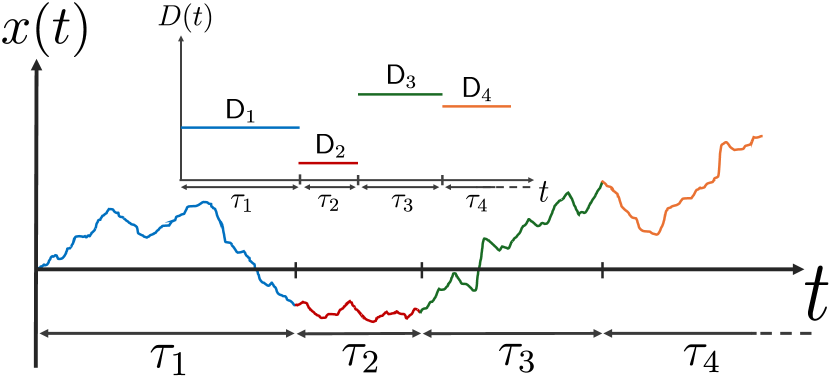
Figure 1: Trajectory of a switching diffusion process in one-dimension. During each time interval $\tau_{i}$, the particle performs an independent Brownian motion with a diffusion constant ${\sf D}_{i}$. In the model studied here, the $\tau_{i}$’s are independent exponential random variables, while the ${\sf D}_{i}$’s, which are also independent, are drawn from an arbitrary distribution $W(D)$.

In this Letter, we consider a model in which a particle, starting from the origin, performs a standard one-dimensional Brownian motion with a diffusion constant ${\sf D}_{1}$ over a time $\tau_{1}$. Both ${\sf D}_{1}$ and $\tau_{1}$ are random variables drawn from a joint distribution $P_{\rm joint}(D,\tau)$. After this time $\tau_{1}$, the particle resumes its motion from its current position, now performing a new Brownian motion with diffusion constant ${\sf D}_{2}$ for a duration $\tau_{2}$, which are drawn independently from the same distribution $P_{\rm joint}(D,\tau)$ as ${\sf D}_{1}$ and $\tau_{1}$. This process continues iteratively for a fixed period of time $t$ (see Fig. 1 for an illustration of this process). Such models have been used to model recent experiments on cytoplasmic membranes (which control the movement of substances in and out of a cell) showing patches of strongly varying diffusivity Serge2008 ; English2011 ; Masson2014 ; Weron2017 . Here we will mainly consider a simpler version of this model where ${\sf D}_{i}$’s and $\tau_{i}$’s are independent, that is, $P_{\rm joint}(D,\tau)=W(D)\,p(\tau)$. More specifically, we will study the case where the $\tau_{i}$’s are exponential random variables with a rate $r$, i.e., $p(\tau)=r\,e^{-r\tau}$, while $W(D)$ is an arbitrary probability distribution function (PDF). A well-known example is the case where $W(D)$ is a superposition of Dirac delta peaks, i.e. $W(D)=\sum_{i=1}^{N}\,p_{i}\,\delta(D-D_{i})$, with $D_{1}>D_{2}>\cdots>D_{N}$ and $\sum_{i=1}^{N}\,p_{i}=1$. This model, sometimes called “composite Markov process” VanKampen , has been studied in various contexts ranging from disordered systems Luczka1 , biophysics Holcman2009 ; Bressloff2017 ; Metzler2023 ; natureGprotein , nuclear magnetic resonance Karger1985 , finance Naik or movement ecology Morales2004 ; Fagan2020 . In the latter, mixtures of random walks with switching dynamics between them are widely used to model intermittent searches where an animal/a particle can employ different motion modes Morales2004 ; Benichou2011 . In the case $N=2$ (referred to as the two-state model), the mode with $D=D_{2}<D_{1}$ would then model local search, while the one with $D=D_{1}$ corresponds to an exploratory motion with larger displacements. Incidentally, this model with $N=2$ recently appeared in the context of stochastic resetting with two resetting points Boyer2024 . Besides the case of discrete diffusion modes, various studies, both theoretical ATTM ; Manzo2015 ; Metzler2023 ; Sposini2018 and experimental Kuhn2011 ; Roichman2020 ; Chubynsky2014 , have considered a continuous distribution for $W(D)$ including exponential and gamma distribution ATTM ; Manzo2015 ; Roichman2020 ; Sposini2018 but also distribution with a finite support Metzler2023 ; Chubynsky2014 .

Summary of our main results. It is useful to summarize our main results. First, for this class of models illustrated in Fig. 1, we have obtained an exact analytical expression for the moments of the positions $\langle x^{2n}(t)\rangle$ of arbitrary order $n$ at any finite time $t$ and for any distribution $W(D)$ which we assume to have all its moments well defined (note that the odd moments of $x(t)$ vanish by symmetry $x\to-x$). Here the notation $\langle\cdots\rangle$ means a simultaneous average over all the sources of randomness on the same footing (i.e., in the language of disordered systems, we consider here an “annealed” average). They read

$$\langle x^{2n}(t)\rangle = \frac{1}{r^{n}}\,\sum_{m=1}^{n}\,a_{n,m}(rt)\,\hat{B}_{n,m}\left(\langle D\rangle,\ldots,\langle D^{n-m+1}\rangle\right),$$

$$a_{n,m}(x) = (2n)!\frac{x^{m+n-1}}{(m+n-1)!}\,\,M(n-1,m+n,-x)\;,$$ (1)

where $\hat{B}_{n,m}$ is the ordinary bell polynomial of $n-m$ variables and homogeneous degree $m$ which enters the relation between the cumulants and the moments of a random variable Riordan_book – see also (23). We provide the first moments in Appendix A. In Eq. (1), the function $M(a,b,x)$ denotes the Kummer’s function. Of course the $2n$-th cumulant, denoted here as $\langle x^{2n}(t)\rangle_{c}$, can be formally obtained from (1). However, their large time behavior is more conveniently extracted from the cumulant generating function, which, as shown below, can be computed explicitly. One finds that their asymptotic behaviors at small and large time read

$$\langle x^{2n}(t)\rangle_{c}\simeq\begin{cases}&\frac{(2n)!}{n!}\langle D^{n}\rangle_{c}\,t^{n}\quad,\quad r\,t\ll 1\,,\\ &\\ &\frac{(2n)!}{r^{n-1}}\,\kappa_{n}(D)\,t\quad,\quad\,r\,t\gg 1\;.\end{cases}$$ (2)

In the first line, $\langle D^{n}\rangle_{c}$ denotes the (standard) cumulant of $D$, while the coefficients $\kappa_{n}(D)\neq\langle D^{n}\rangle_{c}$ also depend in a nontrivial way on the moments of $D$. This result (2) clearly shows that, even at large times $t$, the higher cumulants of $x(t)$ grow linearly with time, revealing the presence of non-Gaussian fluctuations in this model. But what are these nontrivial coefficients $\kappa_{n}(D)$ that characterize this linear growth? As we will show, it turns out that they are none other than the free cumulants of $D$, a class of combinatorial objects central to the field of free probability theory, which was originally developed to study non-commuting random variables Voiculescu – see Appendix B. Free probability has become crucial in random matrix theory (RMT) VivoBook ; PottersBouchaud ; GuionnetHouches ; Voiculescu , with applications that have sparked significant interest in both mathematics BianeBook ; BianeQSSEP ; Speicher_book ; Speicher_book2 and physics Burda , in particular in quantum mechanics Bernard1 ; ETHfree . While such free cumulants appeared before in more complicated classical models of interacting particles Bernard2 ; BB24 , their appearance in such a simple single particle model here is highly surprising and intriguing. Although conventional cumulants $\langle D^{n}\rangle_{c}$ are related to the moments $\langle D^{p}\rangle$, with $p=1,\dots,n$ via Bell polynomials (23), free cumulants have a fairly explicit expression in terms of these moments (29). This enables us to compute them explicitly for various distributions of interest SM . For instance, for the two-state model $W(D)=p\delta(D-D_{1})+(1-p)\delta(D)$ with $0\leq p\leq 1$, one has $\langle x^{2}(t)\rangle_{c}\sim 2(pD_{1}+(1-p)D_{2})t$ while the higher cumulants behave for large time as (for $n\geq 2$)

$$\langle x^{2n}(t)\rangle_{c}\approx-(\Delta D)^{n}\frac{(2n)!}{r^{n-1}}\frac{\sqrt{p(1-p)}}{n(n-1)}P_{n-1}^{1}(1-2p)\,t,$$ (3)

where $\Delta D=(D_{1}-D_{2})$ and $P_{n}^{m}(z)$ denotes the associated Legendre polynomial of degree $n$ and parameter $m$. It is also interesting to study the case where $W(D)$ is a continuous PDF with a finite support, as discussed e.g. in Metzler2023 ; Chubynsky2014 . For example, we consider the case where $W(D)$ is given by the Wigner semi-circle on $[0,D_{\text{max}}]$, i.e.,

$$W(D)=\frac{8}{\pi{D^{2}_{\text{max}}}}\sqrt{D(D_{\max}-D)}\,,$$ (4)

for which it is well known, from RMT, that the corresponding free cumulants are quite simple SM , i.e., $\kappa_{n}(D)=0$ for $n\geq 3$. In this case one finds

$$\langle x^{2}(t)\rangle_{c}\approx D_{\text{max}}t\quad,\quad\langle x^{4}(t)\rangle_{c}\approx\frac{3}{2}\,\frac{D^{2}_{\text{max}}}{r}t\;,$$ (5)

while higher order cumulants vanish to leading order in $t$ [see Eq. (2)]. In fact, for $n\geq 3$, $\langle x^{2n}(t)\rangle_{c}=O(1)$ can also be computed SM . For such a distribution, the non-Gaussianities are somewhat weaker since only the kurtosis is growing with time, while higher order cumulants are simply constant.

What about the full distribution of $x(t)$, both at short and large times? At short time $rt\ll 1$, the particle does not have enough time to switch states and hence diffuses freely with a propagator $e^{-x^{2}/(4{\sf D}_{1}\tau)}/\sqrt{4\pi{\sf D}_{1}\tau}$. Averaging over ${\sf D}_{1}$ leads to

$$\hskip-5.69046ptp_{r}(x,t)\approx\frac{1}{\sqrt{t}}f\left(\frac{x}{\sqrt{t}}\right)\,,\,f(u)=\int\frac{e^{-\frac{u^{2}}{4D}}}{\sqrt{4\pi D}}W(D)\,dD\;.$$ (6)

Not surprisingly, this PDF (6) has exactly the form found for diffusing diffusivity model Chubynsky2014 ; Wang2012 . On the other hand, at large time $r\,t\gg 1$, one finds that the PDF of the position takes a large deviation form

$$p_{r}(x,t)\approx e^{-t\,I\left(y={x}/{t}\right)}\;,$$ (7)

where $I(y)$ is a large deviation function (LDF), whose precise shape depends on $W(D)$. However, its asymptotic behaviors for small and large arguments are universal and are given by

$$I(y)\approx\begin{cases}&\frac{y^{2}}{4\langle D\rangle}\quad\quad\quad\;,\quad y\to 0\;,\\ &r+\frac{y^{2}}{4D_{\max}}\quad,\quad y\to\infty\;.\end{cases}$$ (8)

Here, $D_{\max}$ denotes the right edge of the support of $W(D)$ Note1 . These two asymptotic behaviors can be physically understood as follows. When $y\to 0$, i.e. $x\ll t$, the Gaussian behavior near the center of the PDF picks up the average $\langle D\rangle$ (since there are many switchings, the particle samples the average of $D$). On the other hand, for $y\to\infty$, i.e., $x\gg t$, this behavior is due to very rare trajectories where the particle diffuses with the largest diffusion constant $D_{\rm max}$ without undergoing any switch, which occurs with a probability $e^{-rt}$. Hence, $x\sim O(t)$ acts like a separatrix between typical and atypical trajectories. A similar scenario also occurs in the case of the resetting Brownian motion MSS ; resettingReview or for Brownian particle with a nonzero death rate YMS . As we show below, for some distributions $W(D)$, these two asymptotic behaviors (8) are separated by a transition point where the function $I(y)$ displays a singularity, signaling the presence of a dynamical transition. In some cases, like in the two-state model, there may even be two transitions (see Fig. 2).

Renewal approach. Our approach is based on a renewal argument which allows us to write an exact equation for $p_{r}(x,t)$ which denotes the PDF of the position of the particle at time $t$. It reads SM

$$p_{r}(x,t)=e^{-r\,t}\int_{0}^{\infty}dD\,W(D)\,\frac{e^{-\frac{x^{2}}{4Dt}}}{\sqrt{4\pi Dt}}\,$$ (9)

$$\hskip-14.22636pt+r\hskip-2.84544pt\int_{0}^{t}\hskip-5.69046ptd\tau\hskip-2.84544pt\int_{0}^{\infty}\hskip-8.5359ptdD\,e^{-r\tau}\,W(D)\int_{-\infty}^{+\infty}\hskip-5.69046ptdz\,p_{r}(z,t-\tau)\frac{e^{-\frac{(x-z)^{2}}{4D\tau}}}{\sqrt{4\pi D\tau}}\;.$$

In Eq. (9), the first term represents trajectories where no switching of the diffusion constant occurs. The second term corresponds to the case where there is at least one switching event in $[0,t]$. Suppose that the last switching before $t$ takes place at $t-\tau$, and let $z$ be the position of the walker just before this last switching. Then $p_{r}(z,t-\tau)$ is the propagator until $t-\tau$. After a switching to a new diffusion constant $D$ drawn from $W(D)$ at $t-\tau$, the particle propagates freely during the interval $[t-\tau,t]$ with a Gaussian propagator $e^{-(x-z)^{2}/(4D\tau)}/\sqrt{4\pi D\tau}$. Multiplying these two propagators over $[0,t-\tau]$ and $[t-\tau,t]$, integrating over $z$ and averaging over $D$ drawn from $W(D)$, gives the second term in Eq. (9). In the following, we restrict our analysis to the case where $W(D)$ has a finite support $[0,D_{\text{max}}]$ and refer to SM for more details when the support extends over the full real axis.

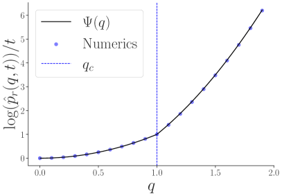
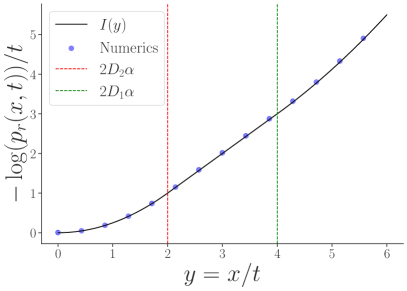
Figure 2: Plot of $\log(\hat{p}_{r}(q,t))/t$ vs $q$ (left panel) and of $-\log(p_{r}(x,t))/t$ vs $y=x/t$ (right panel) for the two-state model. The symbols correspond to numerical results (see SM for details). Left: the solid line shows the exact analytical result $\Psi(q)$ – see Eq. (40). Right: the solid line shows the rate function $I(y)$ given in Eq. (41), displaying two transition points indicated by the dotted lines. The corresponding values of the probabilities are as small as $10^{-2000}$. Here we used $r=1$, $p=10^{-10}$, $D_{2}=1$, $D_{1}=2$ and $t=1000$.

This renewal equation (9) has a convolution structure, both in time and space variables. It is thus natural to introduce the generating function of $x$ together with its Laplace transform (with respect to $t$)

$$\hat{p}_{r}(q,t)=\langle e^{q\,x}\rangle\quad,\quad\tilde{p}_{r}(q,s)=\int_{0}^{\infty}dt\,e^{-st}\hat{p}_{r}(q,t)\;,$$ (10)

where $\langle e^{qx}\rangle=\int_{-\infty}^{\infty}\hskip-2.84544ptdx\,e^{qx}p_{r}(x,t)$. Using the aforementioned convolution structure of (9), $\tilde{p}_{r}(q,s)$ can be computed explicitly, leading to the exact expression

$$\tilde{p}_{r}(q,s)=\frac{J_{r}(q,s)}{1-r\,J_{r}(q,s)}\;,\;J_{r}(q,s)=\int_{0}^{D_{\text{max}}}\hskip-8.5359ptdD\,\frac{W(D)}{r+s-Dq^{2}}.$$ (11)

Note that these functions in the $(q,s)$-plane are defined in the region $r+s>D_{\text{max}}q^{2}$, such that the integrand defining $J_{r}(s,q)$ in (11) is free of any singularity. These formulae (10)-(11) provide an exact representation of the generating function, allowing the computation of the moments given in Eq. (1) – see SM . However, explicitly carrying out the double inversion with respect to $q$ and $s$ to recover $p_{r}(x,t)$ remains a formidable challenge. Despite this difficulty, analytical progress can be made to extract the large-time behavior of $p_{r}(x,t)$. In this regime, the behavior of $\hat{p}_{r}(q,t)$ is governed by the singularities of $\tilde{p}_{r}(q,s)$ in the complex $s$-plane. Indeed, we show that, for large $t$, the generating function $\hat{p}_{r}(q,t)$ reads

$$\hat{p}(q,t)\approx e^{t\,\Psi(q)}\;,\;t\to\infty\;,$$ (12)

where $\Psi(q)=s^{*}(q)$ is the singularity of $\tilde{p}_{r}(q,s)$ with the largest real part in the complex $s$-plane. The function $\Psi(q)$ is a central object since this is the scaled cumulant generating function (SCGF). Indeed, this form in (12) already shows that all the cumulants of $x(t)$ are a priori of order $O(t)$ for large $t$ and given by the behaviors of $\Psi(q)$ near $q=0$, namely $\langle x^{n}(t)\rangle_{c}\approx t\,\partial_{q}^{n}\Psi(q)|_{q=0}$.

Since $\Psi(q)$ is symmetric, we only study it for $q\geq 0$. For sufficiently small $q$, the leading singularity of $\tilde{p}_{r}(q,s)$ in the complex $s$-plane that determines $\Psi(q)$ is a pole, namely a root of the denominator in Eq. (11) SM . Hence, for $q$ small enough, $\Psi(q)=s^{*}(q)$ is given implicitly by the root with the largest real part of the equation

$$1=r\int_{0}^{D_{\text{max}}}dD\frac{W(D)}{r+\Psi(q)-Dq^{2}}\;.$$ (13)

Of course, for general $W(D)$, it seems complicated to compute the derivatives of $\Psi(q)$ explicitly, and get the cumulants from the implicit relation (13). Remarkably, Eq. (13) has a quite familiar structure which is well known in the context of free probability and its application to RMT VivoBook ; PottersBouchaud ; GuionnetHouches ; Voiculescu ; MaidaGuionnet . More precisely the SCGF $\Psi(q)$ is given by (at least in a neighborhood of $q=0$)

$$\Psi(q)=q^{2}\,R\left(\frac{q^{2}}{r}\right)\;,$$ (14)

where $R(z)$ is the so-called R-transform of $W(D)$. Given the PDF $W(D)$, its R-transform is the generating function of the free cumulants $R(z)=\sum_{n\geq 1}z^{n-1}\kappa_{n}(D)$ and it can be obtained from the Cauchy-Stieljes transform of $W(D)$ (see Eq. (36) of Appendix C). This result (14) thus leads to the second line of Eq. (2). Besides, the $O(1)$ correction to the cumulants can also be computed explicitly [see Eq. (38) and Appendix D].

For any discrete or continuous distribution $W(D)$ with a finite support on $[0,D_{\max}]$, the asymptotic behaviors of the SCGF are SM

$$\Psi(q)=\begin{cases}\langle D\rangle\,q^{2}&\;,\quad q\to 0\;,\\ D_{\text{max}}q^{2}-r&\;,\quad q\to\infty\;.\end{cases}$$ (15)

What happens between these two limits depends essentially on the behavior of $W(D)$ near $D_{\max}$, as in the extreme value statistics in the Weibull universality class EVSBook . Let us assume that $W(D)$ behaves as $W(D)\sim(D_{\text{max}}-D)^{\nu}$ when $D\to D_{\text{max}}$ with $\nu>-1$. For $-1<\nu\leq 0$, $\Psi(q)$ is given by Eq. (14) for all $q$ and it is an analytic function of all $q\in\mathbb{R}$. Instead, for $\nu>0$, (14) only holds for small $q$, i.e.,

$$\Psi(q)=\begin{cases}q^{2}\,R\left(\frac{q^{2}}{r}\right)&\;,\quad q<q_{c}\;,\\ D_{\text{max}}q^{2}-r&\;,\quad q>q_{c}\;,\end{cases}$$ (16)

where the SCGF undergoes a transition at $q=q_{c}$, with $q_{c}^{2}=rg(D_{\max})$, $g(x)$ being the Cauchy-Stieltjes transform of $W(D)$ – see Eq. (35). While $\Psi(q)$ is continuous, its higher derivatives display singularities at $q=q_{c}$ (see SM for details). In particular, for $\nu>1$ (as well as for the two-sate model in the limit $p\to 0^{+}$), the first derivative of $\Psi(q)$ is discontinuous – see the left panel of Fig. 2. Interestingly, a very similar transition occurs in the study of Harish-Chandra-Itzykson-Zuber matrix integrals (or spherical integrals) in large dimensions MaidaGuionnet although these two problems are seemingly unrelated.

The LDF $I(y=x/t)$. From the standard theory of large deviations LD_Touchette ; MS17 , namely the Gärtner-Ellis theorem, the exponential form of the SCGF in (12) implies the large deviation form of $p_{r}(x,t)$ in Eq. (7) where the LDF $I(y)$ is given by the Legendre transform of $\Psi(q)$, namely

$$I(y)=\max_{q\in\mathbb{R}}(q\,y-\Psi(q))\;.$$ (17)

Using this formula and the asymptotics of $\Psi(q)$ from Eq. (15), we find that $I(y)$ behaves as in Eq. (8). Since $I(y)$ is symmetric, we study it only for $y\geq 0$.

For a distribution $W(D)$ with a finite support $[0,D_{\max}]$ as discussed above with $-1<\nu\leq 0$, the LDF $I(y)$ is regular and crosses over smoothly between these two asymptotic behaviors in (8). This is, for instance, the case of a uniform distribution SM . However, for $0<\nu<1$, the LDF exhibits a dynamical transition of the form

$$I(y)=\begin{cases}\phi_{\nu}(y)&\quad,\quad y\leq y_{c}=2D_{\max}q_{c}\,,\\ r+\frac{y^{2}}{4D_{\text{max}}}&\quad,\quad y\geq y_{c}\;,\end{cases}$$ (18)

where $\phi_{\nu}(y)$ is the Legendre transform of Eq. (14) – which we can compute explicitly in the case of the Wigner semi-circle law ($\nu=1/2$) SM . Finally, when $\nu>1$, the LDF $I(y)$ exhibits two singular points between which its behavior is linear in $y$, namely

$$I(y)=\begin{cases}\phi_{\nu}(y)&,\quad 0<y<2D_{\rm eff}q_{c}\;,\\ q_{c}y-\gamma&,\quad 2D_{\rm eff}q_{c}<y<y_{c}\;,\\ r+\frac{y^{2}}{4D_{\text{max}}}&,\quad y>y_{c}\;,\end{cases}$$ (19)

where $D_{\rm eff}<D_{\max}$ and $\gamma=D_{\max}q_{c}^{2}-r>0$ can be computed explicitly SM . In SM , we show that the two-state model exhibits the same transitions in the limit $p\to 0^{+}$ – see Appendix E and the right panel of Fig. 2. While $I(y)$ as well as its first derivative is continuous accross the two transitions, the second derivative of $I(y)$ is generically discontinuous at these two points – and similarly at $y=y_{c}$ in Eq. (18) (see SM for more details). The intermediate linear regime, i.e., the second line of (19) corresponds to a pure exponential decay of the form $p_{r}(x,t)\sim e^{-q_{c}x+\gamma t}$. Note that a similar behavior was also found for the large deviation behavior of the PDF of the position of a CTRW Barkai1 ; Sokolov ; Burov1 ; Burov2 . It also bears some similarities with the one found in the context of resetting Brownian motion resettingPRL ; resettingReview ; Kundureset .

Conclusion. We have investigated the dynamics of a Brownian particle with a switching diffusion constant, obtaining the exact expression of the moments at any finite time $t$ and for any $W(D)$ with finite moments. At large times, our analysis of the cumulants and the large deviation function reveals significant deviations from Gaussian behavior in the position distribution of the particle, with intermediate exponential decay emerging in certain cases (19). Remarkably, we uncovered a surprising connection between switching diffusion and free probability theory, an unexpected link in such a classical single particle diffusion model. The origin of this connection remains a challenging and intriguing question for further investigation.

Our work opens several natural extensions. A key question is the generalization to $N$ particles subjected to simultaneous switching dynamics. This direction could build upon recent studies in the context of simultaneous resetting Marco1 ; Marco2 . Similar questions were recently studied for $N$ particles in a harmonic trap in the presence of switching stiffnesses Marco3 and switching centers SabhapanditMajumdar ; KulkarniMajumdar .

Acknowledgments. We thank O. Arizmendi, A. Guionnet, A. Hartmann, M. Maïda, R. Speicher, H. Touchette, L. Touzo and J. B. Zuber for useful discussions. We also acknowledge support from ANR Grant No. ANR- 23-CE30-0020-01 EDIPS.

End Matter

Appendix A: Exact expressions of the first three moments

We present here the first three non-zero moments of the position of the switching diffusion process. These moments are computed directly from the exact expression provided in Eq. (1). They are as follows:

$$\langle x^{2}(t)\rangle = 2\langle D\rangle t,$$ (20)

$$\langle x^{4}(t)\rangle = \frac{e^{-rt}}{r^{2}}\left[12\left(-2+e^{rt}\left(2+rt\left(-2+rt\right)\right)\right)\langle D\rangle^{2}+24\left(1+e^{rt}\left(-1+rt\right)\right)\langle D^{2}\rangle\right],$$ (21)

$$\langle x^{6}(t)\rangle = \frac{120\,e^{-rt}}{r^{3}}\left\{\left[6\left(4+rt\right)+e^{rt}\left(-24+rt\left(18+rt\left(-6+rt\right)\right)\right)\right]\langle D\rangle^{3}\right.$$ (22)

$$\left.+6\left[-2\left(3+rt\right)+e^{rt}\left(6+rt\left(-4+rt\right)\right)\right]\langle D\rangle\langle D^{2}\rangle+6\left(2+rt+e^{rt}\left(-2+rt\right)\right)\langle D^{3}\rangle\right\}\,.$$

These expressions are valid for any distribution $W(D)$ for which the first three moments are well defined.

Appendix B: Cumulants and free cumulants

For a random variable $D$ with distribution $W(D)$, the classical cumulants are related to the moments via the following explicit formula

$$\langle D^{n}\rangle_{c}=\sum_{k=1}^{n}(-1)^{k-1}(k-1)!\,B_{n,k}\left(\langle D\rangle,\ldots,\langle D^{n-k+1}\rangle\right)\,,$$ (23)

where $B_{n,k}$ are the partial exponential Bell polynomials. We give below the first few classical cumulants

$$\langle D\rangle_{c} = \langle D\rangle\,,$$ (24)

$$\langle D^{2}\rangle_{c} = \langle D^{2}\rangle-\langle D\rangle^{2}\,,$$ (25)

$$\langle D^{3}\rangle_{c} = \langle D^{3}\rangle-3\langle D^{2}\rangle\langle D\rangle+2\langle D\rangle^{3}\,,$$ (26)

$$\langle D^{4}\rangle_{c} = \langle D^{4}\rangle-4\langle D^{3}\rangle\langle D\rangle-3\langle D^{2}\rangle^{2}+12\langle D^{2}\rangle\langle D\rangle^{2}-6\langle D\rangle^{4}\,,$$ (27)

$$\langle D^{5}\rangle_{c} = \langle D^{5}\rangle-5\langle D^{4}\rangle\langle D\rangle-10\langle D^{3}\rangle\langle D^{2}\rangle+20\langle D^{3}\rangle\langle D\rangle^{2}+30\langle D^{2}\rangle^{2}\langle D\rangle-60\langle D^{2}\rangle\langle D\rangle^{3}+24\langle D\rangle^{5}\,.$$ (28)

The free cumulants, on the other hand, can be computed using the following explicit formula in terms of the moments of $D$, which reads explicit_free_cumu1 ; explicit_free_cumu2

$$\kappa_{n}(D)=\sum_{j=1}^{n}\frac{(-1)^{j-1}}{j}\binom{n+j-2}{j-1}\widetilde{\sum_{\vec{q}}}\prod_{k=1}^{j}\langle D^{q_{k}}\rangle\,,$$ (29)

where $\widetilde{\sum_{\vec{q}}}$, with $\vec{q}=(q_{1},\cdots,q_{j})$ denotes a constrained sum such that $q_{1}+q_{2}+\ldots+q_{j}=n$ with integers $q_{k}\geq 1$. Note that we have corrected a typo compared to explicit_free_cumu1 ; explicit_free_cumu2 , where instead $q_{k}\geq 0$. When specified to the two-state model, for which $\langle D^{q}\rangle=pD_{1}^{q}+(1-p)D_{2}^{q}$ one obtains, after some manipulations, the formula given in (3). The first few free cumulants are given by

$$\kappa_{1}(D) = \langle D\rangle\,,$$ (30)

$$\kappa_{2}(D) = \langle D^{2}\rangle-\langle D\rangle^{2}\,,$$ (31)

$$\kappa_{3}(D) = \langle D^{3}\rangle-3\langle D^{2}\rangle\langle D\rangle+2\langle D\rangle^{3}\,,$$ (32)

$$\kappa_{4}(D) = \langle D^{4}\rangle-4\langle D^{3}\rangle\langle D\rangle-2\langle D^{2}\rangle^{2}+10\langle D^{2}\rangle\langle D\rangle^{2}-5\langle D\rangle^{4}\,,$$ (33)

$$\kappa_{5}(D) = \langle D^{5}\rangle-5\langle D^{4}\rangle\langle D\rangle-5\langle D^{3}\rangle\langle D^{2}\rangle+15\langle D^{3}\rangle\langle D\rangle^{2}+15\langle D^{2}\rangle^{2}\langle D\rangle-35\langle D^{2}\rangle\langle D\rangle^{3}+14\langle D\rangle^{5}\,.$$ (34)

The expressions for classical and free cumulants differ starting from $n>3$. This is because the computation of the classical cumulant $\langle D^{n}\rangle_{c}$ usually involves a sum over all possible partitions of $\{1,2,\dots,n\}$, including both crossing and non-crossing partitions. In contrast, free cumulants are computed using only non-crossing partitions of the indices Speicher_book .

For $n=1$, $2$, and $3$, the possible partitions of the sets $\{1\}$, $\{1,2\}$, and $\{1,2,3\}$ do not include any crossing partitions. Consequently, for $n\leq 3$ , the set of all partitions coincides with the set of non-crossing partitions Speicher_book , meaning the first three free cumulants are identical to the corresponding classical cumulants.

Appendix C: The SCGF $\Psi(q)$ in terms of the R-transform of $W(D)$

For small values of $q$, we argued that the large time behavior of the generating function of $x$ is $e^{t\Psi(q)}$ where $\Psi(q)$ is solution of the Eq. (13). This equation can also be written in terms of the Cauchy-Stieltjes transform $g(x)$ as

$$\frac{q^{2}}{r}=g\left(\frac{r+\Psi(k)}{q^{2}}\right)\quad\text{where}\quad g(x)=\int_{0}^{D_{\max}}dD\,\frac{W(D)}{x-D}\,.$$ (35)

For a real probability measure $W(D)$, the following relation holds

$$g\left(R(z)+\frac{1}{z}\right)=z\,,$$ (36)

where $R(z)$ is the R-transform of the PDF $W(D)$ Speicher_book ; Speicher_book2 ; Voiculescu ; MingoSpeicher17 ; GuionnetHouches . We recall that it can be written, at small $z$, as an expansion where the coefficients are the free cumulants of $W(D)$, namely $R(z)=\sum_{n\geq 1}z^{n-1}\kappa_{n}(D)$. Therefore, by identifying terms in Eq. (35), we obtain the crucial relation

$$\Psi(q)=\lim_{t\to\infty}\frac{\ln\hat{p}_{r}(q,t)}{t}=q^{2}\,R\left(\frac{q^{2}}{r}\right)=r\sum_{n\geq 1}\left(\frac{q^{2}}{r}\right)^{n}\kappa_{n}(D)\,,$$ (37)

where $\kappa_{n}(D)$ are the free cumulants of a random variable distributed according to $W(D)$.

Appendix D: Expansion of the cumulants at large time up to order $O(1)$

It is possible to derive the $O(1)$ term in the large-time expansion of the cumulants of the position of the particle. As demonstrated in SM , this term can be expressed as a sum involving Bell polynomials, whose arguments are the free cumulants of the random variable $D$, which is distributed according to $W(D)$. The resulting expression is given by

$$\langle x^{n}(t)\rangle_{c}\underset{t\to\infty}{\approx}\frac{(2n)!}{r^{n-1}}\,\kappa_{n}(D)\,t-\frac{(2n)!}{r^{n}}\sum_{m=1}^{n}\frac{1}{m}\hat{B}_{n,m}\left(\tilde{\kappa}_{1}(D),\cdots,\tilde{\kappa}_{n-m+1}(D)\right)+O(e^{-rt})\;,\;\tilde{\kappa}_{n}(D)=(n-1)\kappa_{n}(D)\,.$$ (38)

Appendix E: The SCGF $\Psi(q)$ and LDF $I(y)$ for the two-state model

For the two-state model, the SCGF $\Psi(q)$ can be computed explicitly, leading

$$\Psi(q)=\frac{1}{2}\left((D_{1}+D_{2})q^{2}-r+\Delta(q)\right)\quad,\quad\Delta(q)=\sqrt{\left((D_{2}-D_{1})q^{2}+r\right)^{2}+4(D_{1}-D_{2})prq^{2}}\;.$$ (39)

Interestingly, in the limit $p\to 0^{+}$, $\Psi(q)$ exhibits a transition as $q$ crosses some value $q_{c}=\sqrt{r/(D_{1}-D_{2})}$, namely

$$\lim_{p\to 0^{+}}\,\Psi(q)=\begin{cases}D_{2}\,q^{2}&\;,\quad q<q_{c}\;,\\[10.0pt] D_{1}\,q^{2}-r&\;,\quad q>q_{c}\;.\end{cases}$$ (40)

One also finds that $I(y)$ has a nontrivial limit $p\to 0^{+}$ where it takes the form (see SM for details)

$$I(y)=\begin{cases}\frac{y^{2}}{4D_{2}}&,\quad|y|\leq 2D_{2}q_{c}\,,\\ q_{c}\,|y|-D_{2}\,q_{c}^{2}&,\quad 2D_{2}q_{c}\leq|y|\leq 2D_{1}q_{c}\,,\\ r+\frac{y^{2}}{4D_{1}}&,\quad|y|\geq 2D_{1}q_{c}\;.\end{cases}$$ (41)

Interestingly, although $I(y)$ as well as its first derivative $I^{\prime}(y)$ are continuous at $y=2D_{2}q_{c}$ and $y=2D_{1}q_{c}$, the second derivative $I^{\prime\prime}(y)$ is discontinuous, signaling second order dynamical transitions at these two points.

References

- (1) J. P. Bouchaud, A. Georges, Anomalous diffusion in disordered media: statistical mechanisms, models and physical applications, Phys. Rep. 195, 127 (1990).
- (2) R. Metzler, J. Klafter, The random walk’s guide to anomalous diffusion: a fractional dynamics approach, Phys. Rep. 339, 1 (2000).
- (3) R. Golestanian, Anomalous diffusion of symmetric and asymmetric active colloids, Phys. Rev. Lett. 102, 188305 (2009).
- (4) G. M. Viswanathan, V. Afanasyev, S. V. Buldyrev, E. J. Murphy, P. A. Prince, H. E. Stanley, Lévy flight search patterns of wandering albatrosses, Nature 381, 413 (1996).
- (5) R. N. Mantegna, H. E. Stanley, Introduction to econophysics: correlations and complexity in finance, Cambridge University Press (1999).
- (6) B. Wang, J. Kuo, S. C. Bae, S. Granick, When Brownian diffusion is not Gaussian, Nat. Mater. 11, 481 (2012).
- (7) B. Wang, S. M. Anthony, S. C. Bae, S. Granick,, Anomalous yet Brownian, P. Natl. Acad. Sci. USA 106, 15160 (2009).
- (8) P. Witzel, M. Götz, Y. Lanoiselée, T. Franosch, D. S. Grebenkov, D. Heinrich, Heterogeneities shape passive intracellular transport, Biophys. J. 117, 203 (2019).
- (9) E. Barkai, S. Burov, Packets of diffusing particles exhibit universal exponential tails, Phys. Rev. Lett 124, 060603 (2020).
- (10) A. Pacheco-Pozo, I. M. Sokolov, Large deviations in continuous-time random walks, Phys. Rev. E 103, 042116 (2021).
- (11) O. Hamdi, S. Burov, E. Barkai, Laplace’s first law of errors applied to diffusive motion, Eur. Phys. J. B 97, 1 (2024).
- (12) R. K. Singh, S. Burov, The Emergence of Laplace Universality in Correlated Processes, preprint arXiv:2410.23112 (2024).
- (13) M. V. Chubynsky, G. W. Slater, Diffusing diffusivity: a model for anomalous, yet Brownian, diffusion, Phys. Rev. Lett 113, 098302 (2014).
- (14) V. Sposini, A. V. Chechkin, F. Seno, G. Pagnini, R. Metzler, Random diffusivity from stochastic equations: comparison of two models for Brownian yet non-Gaussian diffusion, New J. Phys. 20, 043044 (2018).
- (15) V. Sposini, D. S. Grebenkov, R. Metzler, G. Oshanin, F. Seno, Universal spectral features of different classes of random-diffusivity processes, New J. Phys. 22, 063056 (2020).
- (16) A. Sergé, N. Bertaux, H. Rigneault, D. Marguet, Dynamic multiple-target tracing to probe spatiotemporal cartography of cell membranes, Nat. methods 5, 687 (2008).
- (17) B. P. English, V. Hauryliuk, A. Sanamrad, S. Tankov, N. H. Dekker, J. Elf, Single-molecule investigations of the stringent response machinery in living bacterial cells, PNAS 108, E365-E373 (2011).
- (18) J. B. Masson, P. Dionne, C. Salvatico, M. Renner, C. G. Specht, A. Triller, M. Dahan, Mapping the energy and diffusion landscapes of membrane proteins at the cell surface using high-density single-molecule imaging and Bayesian inference: application to the multiscale dynamics of glycine receptors in the neuronal membrane, Biophys. J. 106, 74 (2014).
- (19) A. Weron, K. Burnecki, E. J. Akin, L. Solé, M. Balcerek, M. M. Tamkun, D. Krapf, Ergodicity breaking on the neuronal surface emerges from random switching between diffusive states, Sci. Rep. 7, 5404 (2017).
- (20) N. G. Van Kampen, Stochastic Processes in Physics and Chemistry, North-Holland Publishing Co (1992).
- (21) J. Łuczka, On randomly interrupted diffusion, Acta Phys. Pol. B 4, 717 (1993).
- (22) J. Reingruber, D. Holcman, Gated narrow escape time for molecular signaling, Phys. Rev. Lett. 103, 148102 (2009).
- (23) P. C. Bressloff, Stochastic switching in biology: From genotype to phenotype, J. Phys. A 50, 133001 (2017).
- (24) T. Sungkaworn, M. L. Jobin, K. Burnecki, A. Weron, M. J. Lohse, D. Calebiro Single-molecule imaging reveals receptor–G protein interactions at cell surface hot spots, Nature 550, 543 (2017).
- (25) K. Sakamoto, T. Akimoto, M. Muramatsu, M. S. Sansom, R. Metzler, E. Yamamoto,. Heterogeneous biological membranes regulate protein partitioning via fluctuating diffusivity, PNAS Nexus 2, 1 (2023).
- (26) J. Kärger, NMR self-diffusion studies in heterogeneous systems, Adv. Colloid Interfac. 23, 129 (1985).
- (27) V. Naik, Option valuation and hedging strategies with jumps in the volatility of asset returns, J. Financ. 48, 1969 (1993).
- (28) J. M. Morales, D. T. Haydon, J. Frair, K. E. Holsinger, J. M. Fryxell, Extracting more out of relocation data: building movement models as mixtures of random walks, Ecology 85, 2436 (2004).
- (29) W. F. Fagan, T. Hoffman, D. Dahiya, E. Gurarie, R. S. Cantrell, C. Cosner, Improved foraging by switching between diffusion and advection: benefits from movement that depends on spatial context, Theor. Ecol. 13, 127 (2020).
- (30) O. Bénichou, C. Loverdo, M. Moreau, R. Voituriez, Intermittent search strategies, Rev. Mod. Phys. 83, 81 (2011).
- (31) P. Julián-Salgado, L. Dagdug, D. Boyer, Diffusion with two resetting points, Phys. Rev. E 109, 024134 (2024).
- (32) P. Massignan, C. Manzo, J. A. Torreno-Pina, M. F. García-Parajo, M. Lewenstein, G. J. Lapeyre Jr, Nonergodic subdiffusion from Brownian motion in an inhomogeneous medium. Phys. Rev. Lett. 112, 150603 (2014).
- (33) C. Manzo, J. A. Torreno-Pina, P. Massignan, G. J. Lapeyre Jr, M. Lewenstein, M. F. Garcia Parajo, Weak ergodicity breaking of receptor motion in living cells stemming from random diffusivity, Phys. Rev. X 5, 011021 (2015).
- (34) T. Kühn, T. O. Ihalainen, J. Hyväluoma, N. Dross, S. F. Willman, J. Langowski, M. Vihinen-Ranta, J. Timonen, Protein diffusion in mammalian cell cytoplasm, PloS One 6, e22962 (2011).
- (35) I. Chakraborty, Y. Roichman, Disorder-induced Fickian, yet non-Gaussian diffusion in heterogeneous media, Phys. Rev. Research 2, 022020 (2020).
- (36) J. Riordan, An introduction to combinatorial analysis, (John Wiley & Sons, New York, 1958).
- (37) D. V. Voiculescu, K. J. Dykema, A. Nica, Free random variables, (No. 1). American Mathematical Soc. (1992).
- (38) A. Guionnet, Free Probability in Stochastic Processes and Random Matrices, Lecture Notes of the Les Houches Summer School: Volume 104, July 2015
- (39) G. Livan, M. Novaes, P. Vivo, Introduction to random matrices theory and practice, Springer International Publishing (2018).
- (40) M. Potters, J. P. Bouchaud, A first course in random matrix theory: for physicists, engineers and data scientists, Cambridge University Press (2020).
- (41) P. Biane, Free probability for probabilists, Quantum Probability Communications: QP–PQ (Volumes XI) (pp. 55) (2003).
- (42) A. Nica, R. Speicher, Lectures on the combinatorics of free probability, Cambridge University Press (2006).
- (43) R. Speicher, Free probability theory in The Oxford handbook of random matrix theory, Eds. G. Akemann, J. Baik, P. Di Francesco, Oxford University Press (2011).
- (44) P. Biane, Combinatorics of the quantum symmetric simple exclusion process, associahedra and free cumulants, Ann. I. H. Poincaré D, (2023).
- (45) Z. Burda, Free products of large random matrices–a short review of recent developments, J. Phy. Conf. Ser. (Vol. 473, No. 1, p. 012002), IOP Publishing (2013).
- (46) S. Pappalardi, L. Foini, J. Kurchan, . Eigenstate thermalization hypothesis and free probability, Phys. Rev. Lett. 129, 170603 (2022).
- (47) L. Hruza, D. Bernard, Coherent fluctuations in noisy mesoscopic systems, the open quantum ssep, and free probability, Phys. Rev. X 13, 011045 (2023).
- (48) M. Bauer, D. Bernard, P. Biane, L. Hruza, Bernoulli variables, classical exclusion processes and free probability, In Annales Henri Poincaré (Vol. 25, No. 1, pp. 125). Cham: Springer International Publishing (2024).
- (49) P. Bousseyroux, J. P. Bouchaud, An Interacting Particle System Interpretation of Free Convolution, preprint arXiv:2412.03696 (2024).
- (50) M. Guéneau, S. N. Majumdar, G. Schehr, Supplementary Material which also cites Luczka2 ; Ghosh ; Bressloff2states ; Santra ; Grebenkov2019 ; freeBanica ; hartmannreset ; Filon .
- (51) J. Łuczka, M. Niemiec, P. Hänggi, First-passage time for randomly flashing diffusion, Phys. Rev. E 52, 5810 (1995).
- (52) P. K. Ghosh, S. Nayak, J. Liu, Y. Li, F. Marchesoni, Autonomous ratcheting by stochastic resetting, J. Chem. Phy. 159, 031101 (2023).
- (53) P. C. Bressloff, Switching diffusions and stochastic resetting, J. Phys. A: Math. Theor. 53, 275003 (2020).
- (54) I. Santra, U. Basu, S. Sabhapandit, Effect of stochastic resetting on Brownian motion with stochastic diffusion coefficient, J. Phys. A: Math. Theor. 55, 414002 (2022).
- (55) D. S. Grebenkov, Time-averaged mean square displacement for switching diffusion, Phys. Rev. E 99, 032133 (2019).
- (56) T. Banica, Methods of free probability, preprint arXiv:2208.07515 (2022).
- (57) A. K. Hartmann, S. Majumdar, G. Schehr, The distribution of the maximum of independent resetting Brownian motions, In Target Search Problems (pp. 357). Cham: Springer Nature Switzerland (2024).
- (58) L. N. G. Filon, On a quadrature formula for trigonometric integrals, P. Roy. Soc. Edinb. A. 49, 38 (1930).
- (59) If the support of is unbounded, then is infinite.
- (60) S. N. Majumdar, S. Sabhapandit, G. Schehr, Dynamical transition in the temporal relaxation of stochastic processes under resetting. Phys. Rev. E 91, 052131 (2015).
- (61) M. R. Evans, S. N. Majumdar, G. Schehr, Stochastic resetting and applications, J. Phys. A: Math. Theor. 53, 193001 (2020).
- (62) Y. R. Yerrababu, S. N. Majumdar, T. Sadhu, Dynamical phase transitions in certain non-ergodic stochastic processes, preprint arXiv:2412.19516 (2024).
- (63) A. Guionnet, M. Maïda, A Fourier view on the R-transform and related asymptotics of spherical integrals, J. Funct. Anal. 222, 435 (2005).
- (64) S. N. Majumdar, G. Schehr, Statistics of Extremes and Records in Random Sequences, Oxford University Press (2024).
- (65) H. Touchette, The large deviation approach to statistical mechanics, Phys. Rep. 478, 1-69 (2009).
- (66) S. N. Majumdar, G. Schehr, Large deviations, preprint arXiv:1711.07571 (2017).
- (67) M. R. Evans, S. N. Majumdar, Diffusion with stochastic resetting, Phys. Rev. Lett 106, 160601 (2011).
- (68) D. Gupta, A. Pal, A. Kundu Resetting with stochastic return through linear confining potential, J. Stat. Mech. 043202 (2021).
- (69) M. Biroli, H. Larralde, S. N. Majumdar, G. Schehr, Extreme statistics and spacing distribution in a Brownian gas correlated by resetting, Phys. Rev. Lett. 130, 207101 (2023).
- (70) M. Biroli, M. Kulkarni, S. N. Majumdar, G. Schehr, Dynamically emergent correlations between particles in a switching harmonic trap, Phys. Rev. E 109, L032106 (2024).
- (71) M. Biroli, H. Larralde, S. N. Majumdar, G. Schehr, Exact extreme, order, and sum statistics in a class of strongly correlated systems, Phys. Rev. E 109, 014101 (2024).
- (72) S. Sabhapandit, S. N. Majumdar, Noninteracting particles in a harmonic trap with a stochastically driven center, J. Phys. A: Math. Theor. 57, 335003 (2024).
- (73) M. Kulkarni, S. N, Majumdar, S. Sabhapandit, Dynamically emergent correlations in bosons via quantum resetting, preprint arXiv:2407.20342 (2024).
- (74) I. W. Mottelson, Introduction to non-commutative probability, https://web.math.ku.dk/~musat/Free%20probability%20project_final.pdf (2012).
- (75) J. Pielaszkiewicz, D. von Rosen, M. Singull, Cumulant-moment relation in free probability theory, ACUTM 18, 265 (2014).
- (76) J. A. Mingo, R. Speicher, Free probability and random matrices (Vol. 35), New York: Springer (2017).