Global phase portraits of a predator-prey system
Abstract
We classify the global dynamics of a family of Kolmogorov systems depending on three parameters which has ecological meaning as it modelizes a predator-prey system. We obtain all their topologically distinct global phase portraits in the positive quadrant of the Poincaré disc, so we provide all the possible distinct dynamics of these systems.
keywords:
Predator-prey system , Kolmogorov system , global phase portrait , Poincaré disc.1 Introduction
Rosenzweig and MacArthur introduced in [8] the following predator-prey model
where the dot as usual denotes derivative with respect to the time , denotes the prey density (#/unit of area) and denotes the predator density (#/unit of area), the parameter is the death rate of the predator, the function is the # prey caught per predator per unit time, the function is the growth of the prey in the absence of predator, and is the rate of conversion of prey to predator.
The Rosenzweig and MacArthur system is a particular system of the general predator–prey systems with a Holling type II, see [2, 3].
In [4] Huzak reduced the study of the Rosenzweig and MacArthur system to study a polynomial differential system. In order to do that the first step is to do the rescaling . After denoting again by and doing a time rescaling multiplying by , the obtained polynomial differential system of degree three is
| (1.1) |
where and are positive parameters. This system is studied in the positive quadrant of the plane where it has ecological meaning. See systems (1.1) and (2.2) of [4].
Huzak [4] focuses his work in the study of the periodic sets that can produce the canard relaxation oscillations after perturbations. He finds three types of limit periodic sets and studies their cyclicity by using the geometric singular perturbation theory and the family blow-up at , where is the singular perturbation parameter. He proves that the upper bound on the number of limit cycles of the system is 1 or 2 depending on the parameters.
Systems (1.1) are particular Kolmogorov systems. These systems were proposed in 1936, see [5], as an extension of the Lotka-Volterra systems to arbitrary dimension and arbitrary degree.
We want to complete the study of the dynamics of systems (1.1) and classify all their phase portraits on the closed positive quadrant of the Poincaré disc, in this way we also can control the dynamics of the system near the infinity. This classification is given in the following result, except for the case with the parameters satisfying , and , in which we make a conjecture about the expected global phase portrait.
Theorem 1.1.
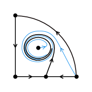
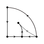
The global phase portait of system (1.1) in the closed positive quadrant of the Poincaré disc is topologically equivalent to one of the phase portraits of Figure 1 in the following way:
-
•
If the phase portrait is equivalent to phase portrait (A).
-
•
If and the phase portrait is equivalent to phase portrait (B).
-
•
If and and the phase portrait is equivalent to phase portrait (C).

Conjecture.
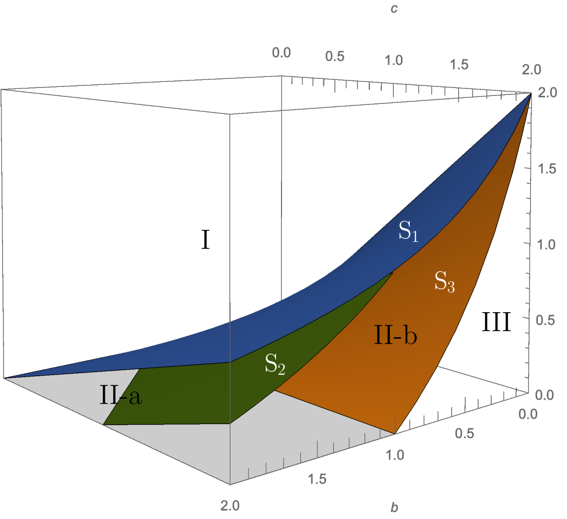
In Figure 2 are represented the regions and surfaces in the parameters space in which each one of the phase portraits are realised. In the region I and over the surface the phase portrait is the one in Figure 1(A) and in the region III the phase portrait is the one in Figure 1(B). In region II there are two subregions, II-a and II-b. It is proved that in the region II-a the phase portrait is the one in Figure 1(C) and we conjecture that the phase portrait is the same in the region II-b and over the surfaces and .
.
2 Preliminaries
Here we introduce the Poincaré compactification, as it allows to control the dynamics of a polynomial differential system near the infinity.
Consider a polynomial system in
of degree ; the sphere , which we will call the Poincaré sphere, and its tangent plane at the point which we identify with .
We can obtain an induced vector field in by means of central projections and , which are defined as
where . The differential and provide a vector field in the northern and southern hemisphere respectively. The points of the equator of correspond with the points at infinity of , and we can extend analytically the vector field to these points of the equator multiplying the field by . This extended field is called the Poincaré compactification of the original vector field. Then we must study the dynamics of the Poincaré compactification near , for studying the dynamics of the original field in the neighborhood of the infinity.
We will work in the local charts and of the sphere , where , , and for with for and .
The expression of the Poincaré compactification in the local chart is
| (2.1) |
in the local chart is
| (2.2) |
and in the local chart the expression is
| (2.3) |
The expression for the Poincaré compactification in the local charts , with is the same as in the charts multiplied by .
As we want to study the behaviour near the infinity, we must study the infinite singular points, i.e., the singular points of the Poincaré compactification which lie in the equator . Note that it will be enough to study the infinite points on the local chart and the origin of the local chart , because if is an infinite singular point, then is also an infinite singular point and they have the same or opposite stability depending on whether the system has odd or even degree.
We shall present the phase portraits of the polynomial differential systems (1.1) in the Poincaré disc, i.e. the orthogonal projection of the closed northern hemisphere of onto the plane . This will be enough since the orbits of the Poincaré compactification on are symmetric with respect to the origin of so we only need to consider the flow in the closed northern hemisphere.
See chapter 5 of [1] for more details about the Poincaré compactification.
3 Finite Singular Points
First we study the finite singular points of system (1.1) in the closed positive quadrant. The origin and the point are singular points for any values of the parameters, and is a positive singular point if and . Note that if then .
Now we study the local phase portraits at these singular points. The origin is a saddle point, as the eigenvalues of the Jacobian matrix at this point are and . At the point the eigenvalues are and . The first eigenvalue is always negative, but we distinguish three cases depending on the second one. If then is a stable node; if then is a saddle (this was the case in [4] because there was kept very small). If , then is a semi-hyperbolic singular point, so from [1, Theorem 2.19] we obtain that is a saddle-node.
At the singular point the eigenvalues of the Jacobian matrix are
where
If then the eigenvalues are complex. In this case for the singular point is an unstable focus, and for it is a stable focus. We deal with this case in Section 6, where we study the Hopf bifurcation which takes place at .
If we have and in this case cannot be zero, because if then , and replacing this expression , so one of the conditions or must hold, but this is a contradiction as from the hypotheses, and if then again in contradiction with the hypotheses. Then and its sign determines if the singular point is either a stable or an unstable node.
If both eigenvalues are real. The determinant of the Jacobian matrix is
which is positive because the singular point exists only if condition holds. Then both eigenvalues are nonzero and have the same sign, particularly, if both are positive and is an unstable node, and if both are negative and is a stable node.
The local phase portrait of the singular point in the case with will be proved in Subsection 6.1.
In summary, we describe in Table 1 the finite singular points according the values of the parameters , and .
| Case | Conditions | Finite singular points |
|---|---|---|
| 1 | . | saddle, stable node. |
| 2 | . | saddle, saddle-node. |
| 3 | , , . | saddle, saddle, unstable node. |
| 4 | , , . | saddle, saddle, stable node. |
| 5 | , , . | saddle, saddle, unstable focus. |
| 6 | , , . | saddle, saddle, stable focus. |
| 7 | , , . | saddle, saddle, weak stable focus. |
4 Infinite Singular Points
In this section we will consider the Poincaré compactification of system (1.1) as it allows to study the behavior of the trajectories near infinity.
In the chart system (1.1) writes
| (4.1) |
The only singular point over is the origin of , which we denote by . The linear part of system (4.1) at the origin is the identity matrix, so is an unstable node.
In the chart system (1.1) writes
| (4.2) |
The origin of is a singular point, , and the linear part of system (4.2) at is identically zero, so we must use the blow-up technique to study it. We do a horizontal blow up introducing the new variable by means of the variable change , and get the system
| (4.3) |
Now rescaling the time variable we cancel the common factor , getting the system
| (4.4) |
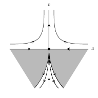
The only singular point on is the origin, which is semi-hyperbolic. Applying [1, Theorem 2.19] we conclude that it is a saddle-node. Studying the sense of the flow over the axis we determine that the phase portrait around the origin of system (4.4) is the one on Figure 3(a). If we multiply by the sense of the orbits on the third and fourth quadrants changes and all the points of the -axis become singular points. With these modifications we obtain the phase portait for system (4.3), given in Figure 3(b). Then we undo the blow up going back to the -plane. We must swap the third and fourth quadrants and shrink the exceptional divisor to the origin. The phase portrait obtained for system (4.2) is not totally determined in the shaded regions of the third and fourth quadrants, see Figure 3(c). This can be solved by doing a vertical blow up but, in our case, it is not necessary because we only need to know the phase portrait of in the positive quadrant of the Poincaré disc, which corresponds with the positive quadrant in the plane , in which the phase portrait is well determined.


As a conclusion the local phase portrait at the infinite singular points is the same independently of the values of the parameters, so in all cases of Table 1 the origin of the chart , i.e. the singular point , is an unstable node and the origin of the chart , i.e. the singular point has only one hyperbolic sector on the positive quadrant of the Poincaré disc being one separatrix at infinity and the other on .
5 Cases with no singular points in the positive quadrant
In the two first cases of Table 1 there is no singular points in the positive quadrant. The finite singular points are the origin and which are both over the axes. The axes are invariant lines so there cannot exist a limit cycle surrounding these singular points. Therefore as we have determined the local phase portrait at the finite and infinite singularities, and we know there are no limit cycles, we can study the global portrait in the first quadrant of the Poincaré disc.
In both cases we obtain the same result since in the case in which is a saddle-node, studying the sense of the flow we determine that the parabolic sector of the saddle-node is always on the positive quadrant of the Poincaré disc. Analysing all the possible alpha and omega-limits, the only possibility is that all the orbits leave the infinite singular point and go to the finite singular point . This phase portait is given in Figure 1 (A).
6 Cases with singular points in the positive quadrant
6.1 Existence of limit cycles
Theorem 6.1.
If and , then there exists at least one limit cycle surrounding singular point .
Proof.
If conditions and hold, then we have case 3 or 5 of Table 1. In both cases singular point is a saddle which has an unstable separatrix on the positive quadrant, is either an unstable node or an unstable focus, and is an unstable node. By Poincaré-Bendixon theorem, there must exists at least one limit cycle which is the -limit of the orbits leaving , the orbits leaving and the separatrix of , as there are no other singular points that can be the -limit of all these orbits. ∎
In cases 5, 6 and 7 of Table 1 the Jacobian matrix at the point has complex eigenvalues because . In these cases we study the existence of Hopf Bifurcation, leading to the following result.
Theorem 6.2.
The equilibrium of system (1.1) undergoes a supercritical Hopf bifurcation at . For the system has a unique stable limit cycle bifurcating from the equilibrium point .
Proof.
The Jacobian matrix at this equilibrium is
and it has eigenvalues , where
| (6.1) |
We get for
| (6.2) |
We are working under condition and from this condition it can be deduced that , so the expression of obtained is positive. Therefore at the equilibrium point has a pair of pure imaginary eigenvalues and the system will have a Hopf bifurcation if some Lyapunov constant is nonzero and .
The equilibrium is stable for (i.e. for ) and unstable for (i.e. for ). In order to analyze this Hopf bifurcation we will apply [6, Theorem 3.3], so we must prove if the genericity conditions are satisfied. We check that the transversality condition is satisfied as
| (6.3) |
and the sign is determined because .
To check the second condition we must compute the first Lyapunov constant. We fix the value and then the equilibrium has the expression
| (6.4) |
We translate to the origin of coordinates obtainig the system
| (6.5) |
which can be represented as
| (6.6) |
where and the multilinear functions and are given by
We need to find two eigenvectors of the matrix verifying
as for example
| (6.7) |
Now we compute
and the first Lyapynov coefficient
which is negative for any values of the parameters, and so the second condition of the theorem we are applying is satisfied and we can conclude that a unique stable limit cycle bifurcates from the equilibrium point through a Hopf Bifurcation for with sufficiently small. ∎
Proposition 6.3.
If and , the limit cycle surrounding singular point is unique.
Proof.
This result follows from [7] by proving that system (1.1) with and satisfies conditions (i)-(iv) in Section 2 of [7].
Condition (i) holds taking which verifies and for all as we have assumed .
Condition (ii) holds for , and . From condition we deduce that
and condition guarantees that .
Condition (iii) holds for and . It can be proved that with the expressions chosen for and the condition , is equivalent to the condition :
Condition (iv) is satisfied with
We have
| (6.8) |
which is always negative as the polynomial in the numerator is negative in and has no real roots.
Then, as conditions (i)-(iv) hold for our systems, we can conclude that the limit cycle is unique. ∎
Remark 6.4.
So far we have not proved if in cases 4, 6, and 7 of Table 1 there are or not limit cycles. The following result proves that in some subcases there are not limit cycles.
Theorem 6.5.
If , and , then system (1.1) does not have periodic orbits in the set .
Proof.
Let
In order to prove the non existence of periodic orbits we use Bendixson-Dulac Theorem that states that if there exists a function such that the term
does not change sign in a simply connected set , then there are no
periodic orbits on .
We consider the function , then:
We observe that there are no periodic orbits in the set
because for all the points in this set and for the same reason there are no periodic orbits crossing the line . As a consequence we can restrict to the case for which we obtain
Then in if and we conclude that there are no periodic orbits in the whole set .
∎
Conjecture.
If , (i. e, we are in cases 4,6, or 7 of Table 1) and , there are not limit cycles.
We have numerical evidences that the conjecture holds.
6.2 Phase portraits on the positive quadrant of the Poincaré disc
Now we study the global phase portraits of system (1.1) on the positive quadrant of the Poincaré disc when there is a singular point in the positive quadrant, assumming the previous Conjecture.
In case 3 of Table 1, by Theorem 6.1 there exist a unique limit cycle which is the -limit of all orbits leaving and , and also the -limit of the unstable separatrix leaving in the positive quadrant. Then the global phase portraits is the one on Figure 1(B).
In case 5 of Table 1 we have again that there exists a unique limit cycle attracting all orbits in the positive quadrant. The global phase portrait is the same as the one in case 3 but here the singular point in the positive quadrant is an unstable focus instead of an unstable node. As the local phase portraits of these two singular points are topologically equivalent we have again phase portrait (B) of Figure 1.
In cases 4, 6 and 7 of Table 1, if we have proved that there are no limit cycles. In case 4 the only possibility is that the stable node is a global attractor for all orbits in the positive quadrant, and we have the global phase portrait given in Figure 1(C). In cases 6 and 7 of Table 1, is a stable focus and attracts all the orbits of the positive quadrant. As the local phase portrait of a stable focus is topologically equivalent to a stable node, we also have here the phase portrait of Figure 1(C).
In the cases 4, 6 and 7 of Table 1, if the conditions does not hold, we have asummed that there are not limit cycles, so the conjectured phase portraits will be the same.
Acknowledgements
The first and third authors are partially supported by the Ministerio de Ciencia e Innovación, Agencia Estatal de Investigación (Spain), grant PID2020-115155GB-I00 and the Consellería de Educación, Universidade e Formación Profesional (Xunta de Galicia), grant ED431C 2019/10 with FEDER funds. The first author is also supported by the Ministerio de Educacion, Cultura y Deporte de España, contract FPU17/02125.
The second author is partially supported by the Agencia Estatal de Investigación grant PID2019-104658GB-I00, and the H2020 European Research Council grant MSCA-RISE-2017-777911.
References
- [1] F. Dumortier, J. Llibre and J.C. Artés, Qualitative Theory of Planar Differential Systems, UniversiText, Springer-Verlag, New York, 2006.
- [2] C.S. Holling, The components of predation as revealed by a study of small-mammal predation of the European pine sawfly, The Canadian Entomologist 91(5) (1959), 293–320.
- [3] C.S. Holling, Some characteristics of simple types of predation and parasitism, The Canadian Entomologist 91(7) (1959), 385–398.
- [4] R. Huzak, Predator-prey systems with small predator’s death rate, Electronic Journal of Qualitative Theory of Differential Equations 86 (2018), 1–16.
- [5] A. Kolmogorov, Sulla teoria di Volterra della lotta per l’esistenza (in Italian) [On Volterra’s theory of the fight for existence], Giornale dell’ Istituto Italiano degli Attuari 7(1936), 74–80.
- [6] Y. Kuznetsov, Elements of Applied Bifurcation Theory, 2nd ed.; Springer, 1998.
- [7] L. P. Liou and K. S. Cheng, On the uniqueness of a limit cycle for a predator-prey system, SIAM J. Math. Anal 19(4), (1988), 867–878.
- [8] M. Rosenzweig and R. MacArthur, Graphical representation and stability conditions of predator-prey interaction, American Naturalist 97 (1963), 209–223
- [9] J. Alavez-Ramírez, G. Blé, V. Castellanos and J. Llibre, On the global flow of a 3-dimensional Lotka–Volterra system, Nonlinear Analysis, 75 (2012), 4114–4125.
- [10] M. J. Álvarez, A. Ferragut and X. Jarque, A survey on the blow up technique, International Journal of Bifurcation and Chaos, 21(2011), No. 11, 3103–3118.
- [11] A. A. Andronov, E. A. Leontovich, I.J. Gordon and A. G. Maier, Qualitative Theory of Second Order Dynamic Systems, J. Wiley & Sons, 1973.
- [12] P. Breitenlohner, G. Lavrelashvili and D. Maison, Mass inflation and chaotic behaviour inside hairy black holes, Nuclear Physics B 524(1998), 427–443.
- [13] F.H. Busse, Transition to Turbulence Via the Statistical Limit Cycle Route, in:Haken H. (eds) Chaos and Order in Nature. Springer Series in Synergetics,1981 , vol 11. Springer-Verlag, Berlin.
- [14] M. Desai and P. Ormerod, Richard Goodwin: A Short Appreciation, The Economic Journal. 108(1998), No. 450, 1431–1435.
- [15] F. Dumortier, Singularities of vector fields on the plane, Journal of Differential Equations, 23(1977), 53–106.
- [16] G. Gandolfo, Economic dynamics, Fourth edition. Springer, Heidelberg, 2009. xxviii+749 pp.
- [17] G. Gandolfo, Giuseppe Palomba and the Lotka–Volterra equations, Rediconti Lincei. 19(2008), No. 4, 347–357.
- [18] R. M. Goodwin, A Growth Cycle, in: Essays in Economic Dynamics. Palgrave Macmillan, 1967, Cambridge University Press, London.
- [19] G. Laval and R. Pellat, Plasma Physics, in: Proceedings of Summer School of Theoretical Physics, Gordon and Breach, New York, 1975.
- [20] J. Llibre and X. Zhang, Darboux theory of integrability in taking into account the multiplicity, Journal of Differential Equations, 2009, No. 246, 541–551.
- [21] J. Llibre and X. Zhang, Darboux theory of integrability for polynomial vector fields in taking into account the multiplicity at infinity, Bulletin des Sciences Mathématiques, 2009, No. 133, 765–778.
- [22] J. Llibre and X. Zhang, Rational first integrals in the Darboux theory of integrability in , Bulletin des Sciences Mathématiques, 2010, No. 134, 189–195.
- [23] R. M. May, Stability and Complexity in Model Ecosystems, Princeton NJ, 1974.
- [24] L.Markus, Global structure of ordinary differential equations in the plane, Trans. Amer. Math. Soc. 76(1954), 127–148.
- [25] D.A. Neumann, Classification of continuous flows on 2-manifolds, Proc. Amer. Math. Soc. 48(1975), 73–81.
- [26] M. M. Peixoto, Proccedings of a simposium held at the university of Bahia, Acad. Press, New York, 1973, pp. 349–420.
- [27] D. Schlomiuk and N. Vulpe, Global topological classification of Lotka–Volterra quadratic differential systems, Electronic Journal of Differential Equations 2012.
- [28] A. W. Wijeratne, F. Yi and J. Wei, Bifurcation analysis in the diffusive Lotka–Volterra system: an application to market economy, Chaos Solitons Fractals 40 (2009), No. 2, 902–911.