On the Instability of Nesterov’s ODE under Non-Conservative Vector Fields

Abstract

We study the instability properties of Nesterov’s ODE in non-conservative settings, where the driving term is not necessarily the gradient of a potential function. While convergence properties under Nesterov’s ODE are well-characterized for optimization settings with gradient-based driving terms, we show that the presence of arbitrarily small non-conservative terms can lead to instability, a phenomenon previously observed empirically via numerical studies in optimization and game-theoretic problems. Our instability analysis combines multi-time scale techniques, such as averaging via variations of constants formula, and Floquet Theory, focusing on systems where the vector field is linear and its Helmholtz decomposition reveals a non-vanishing non-conservative component. To stabilize the dynamics under non-vanishing non-conservative components, we study a regularization mechanism based on restarting. The resulting system is a hybrid dynamical system that mirrors Nesterov’s ODE during intervals of flow, and implements resets of the momentum state through discrete periodic jumps. For this hybrid system, we establish novel explicit bounds on the resetting period that ensure the decrease of a suitable Lyapunov function, guaranteeing not only stability but also “accelerated” convergence rates under suitable smoothness and strong monotonicity properties on the driving term. Numerical simulations support our theoretical results.

1 Introduction

Nesterov’s Accelerated Gradient Method has been a cornerstone in optimization since its inception in (Nesterov, 1983). Its continuous-time analog, introduced in (Su et al., 2016) and termed the Nesterov’s Ordinary Differential Equation (ODE), has emerged as a powerful tool to study optimization algorithms using a continuous-time dynamical systems point of view (Wibisono et al., 2016). By leveraging the continuous-time framework, recent works have developed new parameter estimation (Gaudio et al., 2020) and optimization algorithms (Franca et al., 2018) and established a unified approach for analyzing acceleration schemes (Shi et al., 2022), leading to a more comprehensive understanding of acceleration in optimization. Nesterov’s ODE is defined by the equation:

$$\ddot{x}+\frac{3}{t}\dot{x}+c\cdot\mathcal{G}(x)=0$$ (1)

where $x\in\mathbb{R}^{n}$ represents the state variable, $\mathcal{G}:\mathbb{R}^{n}\to\mathbb{R}^{n}$ denotes the driving vector field, and $c>0$ is a tunable gain. In conservative settings, where $\mathcal{G}(x)=\nabla f(x)$ for some potential convex function $f$, Nesterov’s ODE achieves accelerated convergence to the minimizer of $f$ with an optimal rate of $O(1/t^{2})$, see (Su et al., 2016).

The success of Nesterov’s method in optimization naturally prompts the exploration of its potential applications to non-conservative settings, where $\mathcal{G}(x)$ is not necessarily expressed as the gradient of a potential function. For example, such settings arise in game theory (Mertikopoulos et al., 2019) and consensus-based distributed optimization (Gharesifard and Cortés, 2014). In game-theoretic settings, it is well-established that for a class of games known as potential games, convergence to suitable equilibria can be achieved through gradient-like dynamics. Similarly, in multi-agent systems with undirected graphs, consensus-like dynamics are often analyzed as gradient-like systems. This naturally raises the question of whether such applications can also benefit from dynamics of the form (1) in scenarios where the game is no longer a potential game or the communication graph of the system is directed.

However, extending Nesterov’s acceleration to these domains faces fundamental challenges. First, the absence of a potential function precludes the study of the ODE within an optimization setup as well as the usage of existing stability results in that domain. Second, while in optimization settings Nesterov’s ODE achieves stability and accelerated convergence rates via the use of dynamic damping of the form $\frac{3}{t}\dot{x}$, these same term turns out to be detrimental in non-conservative settings. For example, our previous works on Nash equilibrium seeking and distributed concurrent learning in (Ochoa and Poveda, 2024) and (Ochoa et al., 2024), revealed that in such scenarios Nesterov’s ODE initially exhibits accelerated convergence, yet the dynamic damping is not sufficient to handle the potentially destabilizing effect of the non-conservative part of $\mathcal{G}$ in (6), leading to instability. Although this phenomenon has been observed in numerical studies, providing a theoretical explanation for the instability has, to the best of our knowledge, remained an open problem.

The main contribution of this paper is to provide a theoretical explanation of the emergent instability phenomenon in Nesterov’s ODE driven by non-conservative mappings. By applying a generalization of the Helmholtz decomposition theorem to $n$ dimensions (Glötzl and Richters, 2023), we employ an averaging approach based on the variations of constants formula (Bullo and Lewis, 2005, Proposition 9.6) to analyze the stability properties of Nesterov’s ODE in non-conservative scenarios. Through the study of the resulting average system and the application of Floquet’s Theorem (Sarychev, 2001, Sec. 19), we show that there exists a subclass of vector fields $\mathcal{G}(x)$ that cannot be expressed as gradients of suitable scalar functions, and for which Nesterov’s ODE no longer renders the set $\mathcal{A}=\{x\in\mathbb{R}^{n}~:~\mathcal{G}(x)=0\}$ stable. To establish instability, our analysis focuses on the case where $\mathcal{G}(x)$ is linear and its conservative part is strongly convex, but when $\mathcal{G}(x)$ cannot be expressed as the gradient of a scalar function. This setting represents a simple yet non-trivial departure from the conservative case and allows us to isolate the effects of non-conservative dynamics on the system’s stability. This analysis constitutes our first contribution.

Our second contribution is the analysis of a hybrid dynamical system that ensures the stability of $\mathcal{A}$ by combining two mechanisms: continuous-time dynamics that mirror Nesterov’s ODE during intervals of flow, and discrete-time momentum-resetting dynamics that are periodically triggered when an auxiliary timer variable $\tau\in\mathbb{R}_{\geq 0}$ reaches the upper bound of a compact interval. The studied mechanism constrains the evolution of Nesterov’s ODE to intervals of flow where we can guarantee the decrease of a suitable Lyapunov function. In contrast to our instability analysis where we only studied linear vector fields, this approach analyses a bigger subclass of nonlinear vector fields that satisfy suitable monotonicity and Lipschitz conditions. Building upon and refining the results in (Ochoa and Poveda, 2024), we characterize quasi-optimal restart conditions and establish improved convergence rates.

The rest of this paper is organized as follows. Section 2 introduces the preliminaries and notation. Section 3 presents the study of Nesterov’s ODE under analytic vector fields using the generalized Helmholtz Decomposition Theorem and transforming the system into a form amenable for multi-time scale analysis via averaging. Section 4 presents our first main result, establishing instability for non-conservative linear maps. Section 5 introduces a regularization based on hybrid dynamical systems, and shows how the proposed approach achieves improved convergence rates under quasi-optimal restarting conditions. Finally, Section 7 concludes the paper and outlines directions for future research.

2 Preliminaries

Notation: Given vectors $u,v\in\mathbb{R}^{n}$, we denote their concatenation as $(u,v)=[u^{\top},v^{\top}]^{\top}$. For a matrix $A\in\mathbb{R}^{n\times n}$, we denote by $\textsf{spec}(A)$ the set of its $n$ eigenvalues, counted with multiplicities. For a set of real numbers $\{a_{k}\}_{k=1}^{n}$, $\textsf{diag}\{a_{k}\}_{k=1}^{n}$ denotes the $n\times n$ matrix whose $i$-th diagonal entry equals $a_{i}$ and all off-diagonal entries are zero. We denote the Euclidean norm of a vector $z\in\mathbb{R}^{n}$ by $|z|_{2}$, and define the minimum distance from $z\in\mathbb{R}^{n}$ to a closed set $\mathcal{A}\subset\mathbb{R}^{n}$ as $|z|_{\mathcal{A}}\coloneqq\min_{s\in\mathcal{A}}|z-s|_{2}$.

A function $\alpha:\mathbb{R}_{\geq 0}\to\mathbb{R}_{\geq 0}$ is said to be of class $\mathcal{K}$ if it is continuous, strictly increasing, and $\alpha(0)=0$. A function $\beta:\mathbb{R}_{\geq 0}\times\mathbb{R}_{\geq 0}\to\mathbb{R}_{\geq 0}$ is said to be of class $\mathcal{KL}$ if for each fixed $t\geq 0$, the map $s\mapsto\beta(s,t)$ belongs to class $\mathcal{K}$, and for each fixed $s\geq 0$, the map $t\mapsto\beta(s,t)$ is decreasing and satisfies $\lim_{t\to\infty}\beta(s,t)=0$.

The radius of convergence of a power series $p(x)=\sum_{n=0}^{\infty}a_{n}(x-b)^{n}$, where $x,b\in\mathbb{R}^{n}$, is a nonnegative real number $r$ for which the series converges if $|x-b|<r$. For a smooth vector-valued function $J:\mathbb{R}^{n}\to\mathbb{R}^{n}$, we denote its gradient as $\nabla J(x)=\left(\frac{\partial J_{1}}{\partial x_{1}}(x),\ldots,\frac{\partial J_{n}}{\partial x_{n}}(x)\right)$, its divergence as $\textsf{div}J(x)\coloneqq\sum_{i=1}^{n}\frac{\partial J_{i}}{\partial x_{i}}(x)$, and define the rotation operator $\overline{\textsf{rot}}\,J$, which maps vector fields to matrix-valued functions, as $(\overline{\textsf{rot}}\,J(x))_{ij}\coloneqq\frac{\partial J_{i}(x)}{\partial x_{j}}-\frac{\partial J_{j}(x)}{\partial x_{i}}$. Analogously, given a matrix-valued function $K:\mathbb{R}^{n}\to\mathbb{R}^{n\times n}$, we define the rotation operator as $\textsf{rot}K(x)=\sum_{j=1}^{n}\left(\frac{\partial K_{1j}}{\partial x_{1}}(x),\ldots,\frac{\partial K_{nj}}{\partial x_{n}}(x)\right)$.

The flow of a vector field $f:\mathbb{R}^{n}\to\mathbb{R}^{n}$ is a function $\Phi^{f}:I\times\mathbb{R}^{n}\to\mathbb{R}^{n}$, where $0\in I\subseteq\mathbb{R}$, that maps each initial condition $x_{0}\in\mathbb{R}^{n}$ to the unique solution of the differential equation $\dot{x}(t)=f(x(t))$ with $x(0)=x_{0}$. To simplify notation, for any $\tau\in I$ we write $\Phi^{f}_{\tau}(\cdot)$ in place of $\Phi^{f}(\tau,\cdot)$. Given a diffeomorphism $\Psi:\mathbb{R}^{n}\to\mathbb{R}^{n}$ and a vector field $f:\mathbb{R}^{n}\to\mathbb{R}^{n}$, we define the pullback of $f$ by $\Psi$, denoted $\Psi^{*}f$, as:

$$(\Psi^{*}f)(x)=\left(\frac{\partial\Psi}{\partial x}^{-1}\circ f\circ\Psi\right)(x),$$ (2)

where $\frac{\partial\Psi}{\partial x}(x)$ represents the Jacobian matrix of $\Psi$ at $x$.

Variation of Constants Formula: In this paper, we analyze Nesterov’s ODE using the variation of constants formula, which relates the flows of perturbed and unperturbed vector fields. Consider two time-dependent vector fields $f,g:\mathbb{R}^{n}\times\mathbb{R}_{\geq 0}\to\mathbb{R}^{n}$, where $g$ represents a perturbation to the nominal field $f$. The variation of constants formula establishes the following relationship between the flows of $f+g$, $f$, and $g$:

Theorem 2.1

(Bullo and Lewis, 2005, Proposition 9.6) Let $g$ be $r$-th and $f$ be $(r+1)$-th continuously differentiable time-dependent vector fields. For $x_{0}\in\mathbb{R}^{n}$, $T>0$, and $\tau\in[0,T]$, let $\Phi^{f}_{\tau}$ be the flow of $f$ from time $0$ to $\tau$. Define $\tilde{g}(\tau,x)=((\Phi^{f}_{\tau})^{*}g_{\tau})(x)$, where $g_{\tau}(x)\coloneqq g(x,\tau)$, and $(\Phi^{f}_{\tau})^{*}g_{\tau}$ denotes the pullback of $g_{\tau}$ along the flow of $f$. Then, for all $\tau\in[0,T]$ where the flows $\Phi^{f+g}_{\tau}$, $\Phi_{\tau}^{f}$, and $\Phi^{\tilde{g}}_{\tau}$ exist, it follows that:

$$\Phi^{f+g}_{\tau}(x_{0})=\left(\Phi^{f}_{\tau}\circ\Phi^{\tilde{g}}_{\tau}\right)(x_{0}).$$ (3)

Equivalently, for solutions $\gamma,\zeta:[0,T]\to\mathbb{R}^{n}$ satisfying:

$$\frac{d\gamma}{d\tau}(\tau) =f(\gamma(\tau),\tau)+g(\gamma(\tau),\tau),\quad\gamma(0)=x_{0},$$

$$\frac{d\zeta}{d\tau}(\tau) =((\Phi^{f}_{\tau})^{*}g_{\tau})(\zeta(\tau)),\quad\zeta(0)=x_{0},$$

their values relate as $\gamma(t)=\Phi^{f}_{t}(\zeta(t))$ for all $t\in[0,T]$. $\square$

Hybrid Dynamical Systems: To study mechanisms capable of recovering the stability of Nesterov’s ODE in non-conservative settings, in this paper we employ hybrid dynamical systems (HDS) with state $x\in\mathbb{R}^{n}$ and dynamics

$$x\in C,~~~\dot{x}\in F(x),$$ (4)

$$x\in D,~~~x^{+}\in G(x),$$ (5)

where $F:\mathbb{R}^{n}\rightrightarrows\mathbb{R}^{n}$ and $G:\mathbb{R}^{n}\rightrightarrows\mathbb{R}^{n}$ are set-valued mappings called the flow map and jump map, respectively, and $C\subset\mathbb{R}^{n}$ and $D\subset\mathbb{R}^{n}$ are called the flow set and jump set. We use the tuple $\mathcal{H}=(C,F,D,G)$ to refer to the data of the HDS. Solutions to HDS are parameterized by continuous-time $t\in\mathbb{R}_{\geq 0}$ and discrete-time $j\in\mathbb{Z}_{\geq 0}$ and thus evolve on hybrid time domains. For a formal definition of solutions to HDS and hybrid time domains, we refer the reader to (Goebel et al., 2012, Sec. 2). Standard continuous-time systems described by ODEs with vector field $f:\mathbb{R}^{n}\to\mathbb{R}^{n}$, such as system (6), can be cast as HDS by setting $C=\mathbb{R}^{n}$, $D=\emptyset$, and $F(x)=\{f(x)\}$. The following stability notions will be used throughout the paper:

Definition 2.1 (Stability Notions)

A compact set $\mathcal{A}\subset C\cup D$ is said to be uniformly globally asymptotically stable (UGAS) for system (4) if $\exists\beta\in\mathcal{K}\mathcal{L}$ such that every solution $x$ satisfies:

$$|x(t,j)|_{\mathcal{A}}\leq\beta(|x(0,0)|_{\mathcal{A}},t+j),\quad\forall(t,j)\in\text{dom}(x),$$

for all $x(0,0)\in\mathbb{R}^{n}$. When $\beta(r,s)=c_{1}re^{-c_{2}s}$ for some $c_{1},c_{2}>0$, the set $\mathcal{A}$ is uniformly globally exponentially stable (UGES). The set $\mathcal{A}$ is unstable for system (4) if there exists $\varepsilon>0$ such that for all $\delta>0$, there exists a solution $x$ to (4) with $|x(0,0)|_{\mathcal{A}}<\delta$ and $(T,J)\in\text{dom}(x)$ satisfying $|x(T,J)|_{\mathcal{A}}>\varepsilon.$ $\square$

3 Nesterov’s ODE: Analysis via Standard Averaging

In this section, we transform Nesterov’s ODE into a form amenable to multi-time scale analysis via averaging. Our derivation consists of two key steps. First, we apply the Helmholtz decomposition theorem to decompose the vector field $\mathcal{G}$ in (6) into its potential and non-conservative components. Second, we employ Theorem 2.1 to express the system in a form suitable for averaging analysis.

Without loss of generality, we begin our analysis by considering a time-shifted variant of Nesterov’s ODE:

$$\frac{d^{2}x}{ds^{2}}+\frac{3}{s+\delta}\frac{dx}{ds}+\mathcal{G}(x)=0,$$ (6)

where $\delta>0$ represents the time-shift parameter. This time shift ensures having well-defined dynamics at $s=0$ while preserving the asymptotic behavior of the original dynamics in (1) through the time transformation $t=s+\delta$.

To analyze the structure of the vector field $\mathcal{G}$, we employ the following generalization of Helmholtz decomposition theorem to $n$-dimensional spaces:

Lemma 3.1

(Glötzl and Richters, 2023, Thm. 7.2) Suppose $\mathcal{G}$ is analytic with infinite radius of convergence. Then, there exists $P:\mathbb{R}^{n}\to\mathbb{R}^{n\times n}$, $J(x)\coloneqq\sum_{k=1}^{n}P_{ii}(x)$, and $K(x)\coloneqq P(x)-P(x)^{\top}$ such that:

$$\mathcal{G}(x)=\nabla J(x)+\textsf{rot}K(x),~\forall x\in\mathbb{R}^{n},$$ (7)

$\textsf{div}\left(\textsf{rot}K(x)\right)=0$, and $\overline{\textsf{rot}}\left(\nabla J\right)=0$. $\square$

Applying this decomposition to (6) yields:

$$\frac{d^{2}x}{ds^{2}}+\frac{3}{t+\delta}\frac{dx}{ds}+c\cdot\nabla J(x)+c\cdot\textsf{rot}K(x)=0.$$ (8)

To ensure a suitable behavior of these components, we impose additional regularity conditions.

Assumption 1

1. Monotonicity: $\exists\kappa_{J}>0$ such that

   $$\left\langle\nabla J(x_{1})-\nabla J(x_{2}),x_{1}-x_{2}\right\rangle\geq\kappa_{J}|x_{1}-x_{2}|^{2},$$

   for all $x_{1},x_{2}\in\mathbb{R}^{n}$. Additionally, we have that

   $$\left\langle\textsf{rot}K(x_{1})-\textsf{rot}K(x_{2}),x_{1}-x_{2}\right\rangle\geq 0$$

   for all $x_{1},x_{2}\in\mathbb{R}^{n}$.

2. Lipschitz continuity: $\exists\ell_{J},\ell_{R}>0$ such that

   $$|\nabla J(x_{1})-\nabla J(x_{2})| \leq\ell_{J}|x_{1}-x_{2}|$$

   $$|\textsf{rot}K(x_{1})-\textsf{rot}K(x_{2})| \leq\ell_{K}|x_{1}-x_{2}|,~\forall x_{1},x_{2}\in\mathbb{R}^{n}.$$

3. Scaling relationship: $\ell_{K}=\alpha\sqrt{\ell_{J}}$ with $\alpha\in(0,1]$. $\square$

The strong monotonicity condition in Assumption 1 ensures that the scalar function $J$ is strongly convex, which, via (Su et al., 2016, Thm. 3), guarantees accelerated convergence of Nesterov’s ODE to the unique minimizer of $J$ when the non-conservative term $\textsf{rot}K$ is not present. The following example illustrates a class of vector fields that satisfies these conditions.

Example 3.1

Given $Q\in\mathbb{R}^{n\times n}$, the vector field $\mathcal{G}(x)=Qx$ is analytic and satisfies Assumption 1. The Helmholtz decomposition (7) can be explicitly constructed by letting

$$J(x) =x^{\top}Q_{s}x,\text{ and }$$

$$(K(x))_{ij} =x_{i}Q_{a}x_{j},\quad\forall x\in\mathbb{R}^{n}\text{ and }i,j\in\{1,2,\ldots,n\},$$

where $Q_{s}\coloneqq\frac{1}{2}(Q+Q^{\top})$ and $Q_{a}\coloneqq\frac{1}{2}(Q-Q^{\top})$ denote the symmetric and skewsymmetric parts of $Q$, respectively. $\square$

Now, by using Assumption 1, we can express (8) in scaled form as follows:

$$\frac{d^{2}x}{ds^{2}}+\frac{3}{s+\delta}\frac{dx}{ds}+c\cdot\ell_{J}\left(\nabla\hat{J}(x)+\frac{1}{\sqrt{\ell_{J}}}\textsf{rot}\hat{K}(x)\right)=0,$$ (9)

where

$$\hat{J}(x)=\frac{1}{\ell_{J}}J(x),\text{ and }\hat{K}(x)=\frac{\alpha}{\ell_{K}}K(x).$$

By introducing the time-scale transformation $\tau=s/\varepsilon$ with $\varepsilon=(\ell_{J})^{-\frac{1}{2}}$ and defining the new state vector $y=(y_{1},y_{2})=(x,\frac{dx}{ds})\in\mathbb{R}^{2n}$, from (9), we obtain

$$\frac{dy}{d\tau} =\begin{pmatrix}y_{2}\\ -c\cdot\nabla\hat{J}(y_{1})\end{pmatrix}+\varepsilon\begin{pmatrix}0\\ -\frac{3}{\varepsilon\tau+\delta}y_{2}-c\cdot\textsf{rot}\hat{K}(y_{1})\end{pmatrix}$$

$$\eqqcolon h(y)+\varepsilon g(y,\varepsilon\tau).$$ (10)

Finally, to arrive at the standard averaging form we let $\Phi_{\tau}^{h}(y_{0})$ denote the solution of $\frac{dy}{d\tau}=h(y)$ at time $\tau$ with initial condition $y_{0}\in\mathbb{R}^{2n}$. For this system, uniqueness of solutions follows from the global Lipschitz property of $h$ under Assumption 1-(ii). Therefore, by using the pullback of $g_{\varepsilon\tau}(y)=g(y,\varepsilon\tau)$ via $\Phi_{\tau}^{h}$ we obtain a continuous-time dynamical system with state $z\in\mathbb{R}^{2n}$ and described by the following ODE:

$$\frac{dz}{d\tau}=\varepsilon\left(\left(\Phi_{\tau}^{h}\right)^{*}g_{\varepsilon\tau}\right)(z)\eqqcolon\varepsilon f(z,\varepsilon\tau,\tau).$$ (11)

By Theorem 2.1, for a solution $y$ to (3) and a solution $z$ to (11) satisfying $y(0)=z(0)$, we have that $y(\tau)=\Phi_{\tau}^{h}\left(z(\tau)\right)$ for all $\tau\in\text{dom}(y)$.

Remark 3.1

The standard averaging form in (11) admits a series representation through the expansion of the pullback in integrals of iterated Lie brackets between $g_{\varepsilon\tau}$ and $h$. The convergence properties of this expansion have been rigorously established in (Agračev and Gamkrelidze, 1979). While obtaining a closed form for this representation is generally intractable, simplifications emerge when certain Lie brackets between $h$ and $g_{\varepsilon\tau}$ vanish—an approach exploited for a subclass of Euler-Lagrange systems in (Bullo, 2002). Although Nesterov’s ODE admits an Euler-Lagrange formulation (see (Wibisono et al., 2016)) that could potentially benefit from similar simplifications, and since our goal is to show instability under non-conservative maps, in this paper we restrict our analysis to the linear case, as in Example 3.1, leaving the general nonlinear case for future work. $\square$

4 Instability under Linear Mappings

In this section, we specialize systems (3) and (11) to the setting where $\mathcal{G}$ has the form $\mathcal{G}(x)=Qx$ for some $Q\in\mathbb{R}^{n\times n}$. In this case, the Helmholtz decomposition yields $J(x)=\frac{1}{2}x^{\top}Q_{s}x$ and $\textsf{rot}K(x)=\frac{1}{2}Q_{a}x$, where $Q=Q_{s}+Q_{a}$ with $Q_{s}$ symmetric and $Q_{a}$ skew-symmetric (see Example 3.1).

Additionally, the scaled Nesterov’s ODE in (3) becomes

$$\frac{dy}{d\tau}=\underbrace{\begin{pmatrix}0&I\\ -c\cdot\hat{Q}_{s}&0\end{pmatrix}}_{\displaystyle\eqqcolon A}y+\varepsilon\underbrace{\begin{pmatrix}0&0\\ -c\cdot\hat{Q}_{a}&-\frac{3}{\varepsilon\tau+\delta}I\end{pmatrix}}_{\displaystyle\eqqcolon B(\varepsilon\tau)}y$$ (12)

where $\hat{Q}_{s}=\frac{Q_{s}}{\|Q_{s}\|}$, and $\hat{Q}_{a}=\alpha\frac{Q_{a}}{\|Q_{a}\|}$, with $\alpha\in(0,1]$. Similarly, the dynamical system in (11) reduces to

$$\frac{dz}{d\tau}=\varepsilon\Lambda(s,\tau)z\coloneqq\varepsilon\left(e^{-A\tau}B(s)e^{A\tau}\right)z,\quad\frac{ds}{d\tau}=\varepsilon,$$ (13)

where we used the fact that $\varepsilon\tau=s$. Before presenting the first main result of this paper, we introduce an auxiliary lemma that, under suitable conditions on $Q_{s}$, shows that the flow along the vector field $y\mapsto Ay$ is periodic.

Lemma 4.1

Let $\mathcal{G}(x)=Qx$ where $Q\in\mathbb{R}^{n\times n}$ and $\mathcal{G}$ satisfies Assumption 1. Suppose that the symmetric part $Q_{s}$ has rational eigenvalues. Then every solution $\psi$ to

$$\frac{d\psi}{d\tau}=A\psi,$$ (14)

where $A$ is defined in (12), is periodic. $\square$

Proof.

The proof follows by direct eigenvalue analysis of the matrix $A$. We present the proof for completeness. First, by the determinant of a $2\times 2$ block matrix, it follows that

$$\text{det}\left(\lambda I-A\right) =\text{det}(\lambda^{2}I+\hat{Q}_{s}).$$

This implies that the eigenvalues of the matrix $A$ are equal to the square root of the eigenvalues of the matrix $-\hat{Q}_{s}$. Since $J(x)=\frac{1}{2}x^{\top}Q_{s}x$ is strongly convex, $\hat{Q}_{s}$ is positive definite, and hence all its eigenvalues are positive. Therefore, all the eigenvalues of $A$ are nonzero and lie in the imaginary axis. Moreover, since $Q_{s}$ has rational eigenvalues, the eigenvalues of $A$ are integer multiples of a common imaginary number. This commensurability of imaginary eigenvalues ensures that every solution to (14) is periodic. ∎

The result of Lemma 4.1 enables the use of techniques for averaging of periodic systems with slow-time dependence (see (Sanders et al., 2007, Section 3.3)), and leads to the first main result of this paper.

Theorem 4.1

Let $\mathcal{G}(x)=Qx$, $Q\in\mathbb{R}^{n\times n}$, and assume $\mathcal{G}$ satisfies Assumption 1. Suppose that: i) all off-diagonal entries of $Q_{a}$ are nonzero, ii) the spectrum of $Q_{s}$ consists of rational eigenvalues, and iii) precisely one eigenvalue of $Q_{s}$ has algebraic multiplicity greater than one. Then, the origin is unstable under Nesterov’s ODE. $\square$

Proof.

We divide the proof in three main steps.

Step 1 (Definition of the Average System): First, via Lemma 4.1, we have that $\Lambda(s,\tau)$ is periodic in $\tau$. Letting $\tilde{T}$ be the associated period, and averaging (13) over $\tau$ we obtain the following slow time-varying average system:

$$\frac{d\zeta}{d\tau} =\varepsilon\overline{\Lambda}(s)\zeta, \frac{ds}{d\tau} =\varepsilon,$$ (15)

where

$$\overline{\Lambda}(t) \coloneqq\overline{B}_{1}+\frac{3}{s+\delta}\overline{B}_{2},~~\overline{B}_{k}\coloneqq{\frac{1}{\tilde{T}}\int_{0}^{\tilde{T}}e^{-A\tau}B_{k}e^{A\tau}},$$

for $k\in\{1,2\}$, and

$$B_{1}\coloneqq\begin{pmatrix}0&0\\ -c\cdot\hat{Q}_{a}&0\end{pmatrix},\quad\text{and }\quad B_{2}\coloneqq\begin{pmatrix}0&0\\ 0&-I\end{pmatrix}.$$

Step 2 (Instability of the Average System): As $t\to\infty$ the dominant term determining the stability of (15) is given by the average $\overline{B}_{1}$. This step analyzes this average using the diagonalizability of $\hat{Q}_{s}$.

Since $\hat{Q}_{s}$ is positive definite, there exists an orthonormal matrix $P$ such that

$$P^{\top}\hat{Q}_{s}P=\textsf{diag}\{q_{k}\}_{k=1}^{n}\eqqcolon\Delta_{s},~q_{k}>0,$$

where $\{q_{k}\}_{k=1}^{n}=\textsf{spec}(\hat{Q}_{s})$, and where $q_{k}>0$ for all $k$ by Assumption 1-(i). Let $\hat{P}\coloneqq I_{2}\otimes P$, where $\otimes$ denotes the Kronecker product, and define

$$\Delta \coloneqq\hat{P}^{\top}A\hat{P}=\begin{pmatrix}0&I\\ -\Delta_{s}&0\end{pmatrix}.$$

It then follows that

$$\hat{P}^{\top}e^{A\tau}\hat{P} =e^{\Delta\tau}=\begin{pmatrix}\mathcal{C}(\tau)&\mathcal{S}_{2}(\tau)\\ -\mathcal{S}_{1}(\tau)&\mathcal{C}(\tau)\end{pmatrix},$$ (16a)

$$\hat{P}^{\top}e^{-A\tau}\hat{P} =e^{-\Delta\tau}=\begin{pmatrix}\mathcal{C}(\tau)&-\mathcal{S}_{2}(\tau)\\ \mathcal{S}_{1}(\tau)&\mathcal{C}(\tau)\end{pmatrix},$$ (16b)

where

$$\mathcal{C}(\tau) \!\coloneqq\!\textsf{diag}\left\{\cos(\lambda_{k}\tau)\right\}_{k=1}^{n},$$

$$\mathcal{S}_{1}(\tau) \!\coloneqq\!\textsf{diag}\left\{\lambda_{k}\sin(\lambda_{k}\tau)\right\}_{k=1}^{n},$$

$$\mathcal{S}_{2}(\tau) \!\coloneqq\!\textsf{diag}\left\{\lambda_{k}^{-1}\sin(\lambda_{k}\tau)\right\}_{k=1}^{n},$$

and $\lambda_{k}\coloneqq\sqrt{q_{k}}$ for all $k=\{1,2,\ldots,n\}$.

Using these definitions, we analyze the term

$$\hat{P}^{\top}\overline{B}_{1}\hat{P}=\frac{1}{\tilde{T}}\int_{0}^{\tilde{T}}e^{-\Delta\tau}\hat{P}^{\top}B_{1}\hat{P}e^{\Delta\tau}d\tau.$$ (17)

By using (16), and letting $\tilde{Q}_{a}\coloneqq P^{\top}\hat{Q}_{a}P$, we write the integrand as follows

$$e^{-\Delta\tau}\hat{P}^{\top}B_{1}\hat{P}e^{\Delta\tau} =c\cdot\begin{pmatrix}\mathcal{S}_{2}(\tau)\tilde{Q}_{a}\mathcal{C}(\tau)&\mathcal{S}_{2}(\tau)\tilde{Q}_{a}\mathcal{S}_{2}(\tau)\\ -\mathcal{C}(\tau)\tilde{Q}_{a}\mathcal{C}(\tau)&-\mathcal{C}(\tau)\tilde{Q}_{a}\mathcal{S}_{2}(\tau)\end{pmatrix}.$$

Then, from the definitions of $C(\tau)$ and $\mathcal{S}_{2}(\tau)$:

$$\left[\mathcal{S}_{2}(\tau)\tilde{Q}_{a}\mathcal{C}(\tau)\right]_{ij} =\lambda_{i}^{-1}\sin(\lambda_{i}\tau)\tilde{Q}_{a,ij}\cos(\lambda_{j}\tau)$$

$$\left[\mathcal{S}_{2}(\tau)\tilde{Q}_{a}\mathcal{S}_{2}(\tau)\right]_{ij} =\lambda_{i}^{-2}\sin(\lambda_{i}\tau)\tilde{Q}_{a,ij}\sin(\lambda_{j}\tau)$$

$$\left[\mathcal{C}(\tau)\tilde{Q}_{a}\mathcal{C}(\tau)\right]_{ij} =\cos(\lambda_{i}\tau)\tilde{Q}_{a,ij}\cos(\lambda_{j}\tau)$$

$$\left[\mathcal{C}(\tau)\tilde{Q}_{a}\mathcal{S}_{2}(\tau)\right]_{ij} =\lambda_{j}^{-1}\cos(\lambda_{i}\tau)\tilde{Q}_{a,ij}\sin(\lambda_{j}\tau).$$

Since the period $\tilde{T}$ can be written as the least common multiple of $\left\{\!\frac{1}{\lambda_{1}},{\cdots},\frac{1}{\lambda_{n}}\!\right\}$, it follows that the terms $\mathcal{C}(\tau)\tilde{Q}_{a}\mathcal{S}_{2}(\tau)$ and $\mathcal{C}(\tau)\tilde{Q}_{a}\mathcal{S}_{2}(\tau)$ vanish under the averaging operation in (17). Therefore,

$$\hat{P}^{\top}\overline{B}_{1}\hat{P} =\frac{c}{2}\begin{pmatrix}0&\overline{Q}_{a}^{(2)}\\ \overline{Q}_{a}^{(1)}&0\end{pmatrix},$$ (18a)

where

$$\left(\overline{Q}_{a}^{(1)}\right)_{ij} =\begin{cases}0\quad&\text{if }i=j~\lor~q_{i}\neq q_{j}\\ -\tilde{Q}_{a,ij}&\text{if }q_{i}=q_{j}\end{cases}$$ (18b)

$$\left(\overline{Q}_{a}^{(2)}\right)_{ij} =\begin{cases}0\quad&\text{if }i=j~\lor~q_{i}\neq q_{j}\\ q_{i}^{-1}\tilde{Q}_{a,ij}&\text{if }q_{i}=q_{j}\end{cases},$$ (18c)

and where we used the fact that $\tilde{Q}_{a}^{\top}=P^{\top}(\hat{Q}_{q})^{\top}P=-P^{\top}\hat{Q}_{a}P=-\tilde{Q}_{a}$ which implies that $\tilde{Q}_{a,ii}=0$ for all $i\in\{1,2,\ldots,n\}$.

Now, by our assumption that the matrix $Q_{s}$ has exactly one degenerate eigenvalue, there exists $q>0$ such that $q_{i}=q$ for all indices $i$ in some subset $\mathcal{I}\subseteq\{1,2,\cdots,n\}$. Additionally, for all pairs of indices $(j,k)$ in the complement set $\mathcal{J}\coloneqq\{1,2,\cdots,n\}\setminus\mathcal{I}$, we have $q_{j}\neq q_{k}\neq q$. Consequently, by equation (18), both matrices $\overline{Q}_{a}^{(1)}$ and $\overline{Q}_{a}^{(2)}$ have zeros in their $j^{th}$ row and $j^{th}$ column for all $j\in\mathcal{J}$. Hence, given $\lambda\in\mathbb{C}$, we obtain that

$$\det(\lambda I-\hat{P}^{\top}\overline{B}_{1}\hat{P})=\lambda^{|\mathcal{J}|}\det\left(\lambda^{2}I+\frac{c}{2q}\tilde{Q}^{2}_{\mathcal{J}}\right),$$ (19)

where $|\mathcal{J}|$ denotes the cardinality of $\mathcal{J}$, and where $\tilde{Q}_{\mathcal{J}}$ is obtained from $\tilde{Q}_{a}$ by removing its $j^{th}$ row and column for every $j\in\mathcal{J}$. Note that $\tilde{Q}_{\mathcal{J}}$ is skew-symmetric by the fact that $\tilde{Q}_{a}$ is skew-symmetric.

By using (19), we obtain that

$$\left\{\lambda\in\mathbb{C}~:~\lambda=\pm\sqrt{\frac{-\mu^{2}}{2q}c},~\mu\in\textsf{spec}(\tilde{Q}_{\mathcal{J}})\right\}\subset\textsf{spec}(\overline{B}_{1}),$$ (20)

where we used the fact that the spectrum of a matrix is invariant under similarity transformations. Since $\tilde{Q}_{\mathcal{J}}$ is skew-symmetric, and given that $Q_{a,ij}\neq 0$ for all $i,j\in\{1,2,\dots,n\}$ by assumption, it follows that there exists a set $\{\omega_{k}\}_{k=1}^{m}\subset\mathbb{R}_{>0}$, with $m=\left\lfloor|\mathcal{J}|/2\right\rfloor$, such that

$$\left\{\pm i\cdot\omega_{k}\right\}_{k=1}^{m}\subseteq\textsf{spec}\left(\tilde{Q}_{\mathcal{J}}\right).$$ (21)

Together, (20) and (21) imply that $\overline{B}_{1}$ has at least one eigenvalue in the right-half side of the complex plane, and thus that the origin is unstable under (15).

Step 3 (Instability of the Original System): Instability of system (13) follows from Step 2 by directly applying the Floquet Theorem presented in (Sarychev, 2001, Sec. 2). To establish the instability of the scaled Nesterov’s ODE in (12), we leverage Theorem 2.1 and note that for all $\tau\in\mathbb{R}_{\geq 0}$:

$$|y(\tau)|=|\Phi^{h}_{\tau}(z)|=|e^{A\tau}z(\tau)|\geq\sigma_{\min}(e^{A\tau})|z(\tau)|$$ (22)

where $\sigma_{\min}(\Lambda)$ denotes the minimum singular value of matrix $\Lambda$. Since $\sigma_{\min}(e^{A\tau})>0$ by the same reasoning used in the proof of Lemma 4.1, the instability of system (13) is implied by the instability of system (12) via (22). ∎

Remark 4.1

Theorem 4.1 provides a theoretical explanation for the phenomenon of instability observed in (Ochoa and Poveda, 2024) and (Ochoa et al., 2024) whenever a non-conservative term appears on the driving mapping $\mathcal{G}$ in (1). Such terms emerge in game-theoretic settings when $\mathcal{G}$ is the pseudo-gradient of a non-potential game, or in multi-agent consensus-based dynamics whenever the graph is directed. Note that the instability emerges irrespective of the size of $Q_{a}$, i.e., even when it is arbitrarily small. $\square$

Remark 4.2

The instability result of Theorem 4.1 also provides a procedure for the synthesis of arbitrarily small, adversarial, state-dependent perturbations able to destabilize (1) under conservative mappings of the form $\mathcal{G}=\nabla J$, even when $J$ is strongly convex. In particular, by adding to $\nabla J$ a perturbation of the form $\textsf{rot}~K(x)$ the resulting system would have the form (9). $\square$

5 Precluding Instability via Restarting

To address the instability arising from the implementation of Nesterov’s ODE under non-conservative mappings, we can regularize the dynamics using resets that restart the momentum. Heuristics that combine momentum-based optimization methods and resets (also called “restarting”) are common in the machine-learning literature, see (O’donoghue and Candes, 2015; Roulet and d’Aspremont, 2017; Kim and Fessler, 2018). Similar approaches have been studied using control-theoretic tools in (Poveda and Li, 2021) and (Teel et al., 2019) under conservative maps, and in (Ochoa and Poveda, 2024) and (Ochoa et al., 2024) for Nash-equilibrium seeking problems in monotone games and for consensus-based decentralized concurrent learning in directed-graphs, respectively. In this section, and compared to previous results, we establish improved convergence rates and tighter resetting conditions for a subclass of vector mappings satisfying Assumption 1-(i) and (ii). The precise conditions defining this subclass will be detailed in Theorem 5.1.

Beginning with Nesterov’s ODE in (1), we introduce a state $\tau\in\mathbb{R}_{\geq 0}$ in place of the continuous time variable $t$ in the dynamic-damping $\frac{3}{t}\dot{x}$. Through the coordinate transformation $q=x$ and $p=\frac{t}{2}\dot{x}+x$, and incorporating $\tau$ as an additional state, the dynamics take the form:

$$\dot{q} =\frac{2}{\tau}(p-q),~~\dot{p}=-2\tau k\cdot\mathcal{G}(q),~~\dot{\tau}=\eta,$$ (23)

where $k=\frac{c}{4}$ and $\eta\in(0,1/2]$ is a parameter governing the evolution of $\tau$. Similar dynamics have been studied in parameter estimation problems for adaptive control, see (Gaudio et al., 2020; Morse, 1992).

To address the instability issues presented in Section 4 for Nesterov’s ODE and thus by the system in (23), we embed the transformed dynamics into a HDS $\mathcal{H}$ of the form (4), with state $\chi=(q,p,\tau)\in\mathbb{R}^{n}\times\mathbb{R}^{n}\times\mathbb{R}_{\geq 0}$, and data $\mathcal{H}=(C,f,D,g)$ defined as follows:

$$C =\{\chi\in\mathbb{R}^{2n+1}:q\in\mathbb{R}^{n},p\in\mathbb{R}^{n},\tau\in[T_{0},T]\}$$ (24a)

$$f(\chi) =\begin{pmatrix}2\tau^{-1}(p-q)\\ -2\tau k\mathcal{G}(q)\\ \eta\end{pmatrix}$$ (24b)

$$D =\{\chi\in\mathbb{R}^{2n+1}:\chi\in C,\tau=T\}$$ (24c)

$$g(\chi) =\begin{pmatrix}q\\ q\\ T_{0}\end{pmatrix}.$$ (24d)

The resulting hybrid mechanism periodically resets $\tau$ to $T_{0}$ when it reaches $T$, preventing the vanishing of the dynamic damping term $\frac{3}{t}\dot{x}$ in the original Nesterov’s ODE. Additionally, by resetting $p$ to $q$ via jumps, we enforce the strong decrease of a suitable Lyapunov function during the discrete-time evolution of the system.

For this HDS, we analyze the stability properties of the compact set $\mathcal{A}\coloneqq\{x^{\star}\}\times\{x^{\star}\}\times[T_{0},T]$, where $x^{\star}\in\mathbb{R}^{n}$ is the unique vector satisfying $\mathcal{G}(x^{\star})=0$. The uniqueness of $x^{\star}$ follows from the strong monotonicity of $\mathcal{G}(\cdot)$, which is implied by the properties of its potential and rotational parts given in Assumption 1 (i) and (ii). The following theorem presents our second main contribution:

Theorem 5.1

Let $\mathcal{G}$ satisfy Assumption 1-(i),(ii). Suppose that $T\in(\underline{T},\theta\overline{T})$ where $\theta\in(0,1)$ and

$$\underline{T}^{2}\coloneqq T_{0}^{2}+\frac{1}{2k\kappa_{J}},~~\text{and}~~\overline{T}^{2}\coloneqq\frac{1}{2k}\frac{\kappa_{J}}{\ell_{K}^{2}}.$$

Then, the set $\mathcal{A}$ is UGES for $\mathcal{H}$. Additionally, for each compact set $K_{0}\subset C\cup D$ there exists $M_{0}>0$ such that every solution $\chi=(q,p,\tau)$ to $\mathcal{H}$ with $\chi(0,0)\in K_{0}$, satisfies the bound

$$|q(t,j)-q^{*}|\leq\frac{T^{2}}{T_{0}^{2}}\sqrt{\frac{\ell_{J}}{\kappa_{J}}}\left(\dfrac{\underline{T}}{\ T\ }\right)^{j/2}M_{0},$$ (25)

for all $(t,j)\in\text{dom}(\chi)$. $\square$

Proof.

Consider the Lyapunov function

$$V(\chi)=\frac{|p-q|^{2}}{4}+\frac{|p-x^{\star}|^{2}}{4}+k\tau^{2}(J(q)-J(x^{\star})).$$

Via Assumption 1-(i), we have that $J$ is strongly convex with Lipschitz continuous gradient. Hence, it follows that $\frac{\kappa_{J}}{2}|q-x^{\star}|\leq J(x)-J(x^{\star})\leq\frac{\ell_{J}}{2}|q-x^{\star}|$. Then, by noting that $|\tau|_{[T_{0},T]}=0$ for all $\chi=(q,p,\tau)\in C\cup D$, there exist $\overline{c}\geq\underline{c}>0$ such that

$$\underline{c}|\chi|^{2}_{\mathcal{A}}\leq V(\chi)\leq\overline{c}|\chi|_{\mathcal{A}}^{2}.$$ (26)

Now, during the flows of $\mathcal{H}$:

$$\dot{V}(\chi)=\langle\nabla_{q}V,\dot{q}\rangle+\langle\nabla_{p}V,\dot{p}\rangle+\langle\nabla_{\tau}V,\dot{\tau}\rangle.$$

We compute $\dot{V}$ element by element:

$$\langle\nabla_{q}V,\dot{q}\rangle =\frac{1}{2}\langle-(p-q)+2k\tau^{2}\nabla J(q),~2\tau^{-1}(p-q)\rangle$$

$$=-\tau^{-1}|p-q|^{2}+2k\tau\langle\nabla J(q),~p-q\rangle$$

$$\langle\nabla_{p}V,\dot{p}\rangle =\frac{1}{2}\big{\langle}(p-q)+(p+q-q-x^{\star}),~-2k\tau\mathcal{G}(q)\big{\rangle}$$

$$=-2k\tau\langle p-q,~\mathcal{G}(q)\rangle-k\tau\langle q-x^{\star},\mathcal{G}(q)\rangle$$

$$\langle\nabla_{\tau}V,\dot{\tau}\rangle \leq\tau k(J(q)-J(x^{\star})).$$

By using these expressions together with the Helmholtz decomposition $\mathcal{G}(q)=\nabla J(q)+\textsf{rot}K(q)$ introduced in Section 3, during the flows of $\mathcal{H}$:

$$\dot{V}(\chi) \leq-\frac{1}{T}|p-q|^{2}-k\tau\langle q-x^{\star},\textsf{rot}K(x)\rangle$$

$$-2k\tau\langle p-q,~\textsf{rot}K(q)\rangle$$

$$-\tau k\Big{(}\langle\nabla J(q),q-x^{\star}\rangle-(J(q)-J(x^{\star}))\Big{)},$$ (27)

where we used the fact that $\tau\leq T$ for all $\chi=(q,p,\tau)\in C$. Now, by the strong convexity of $J$ we have that $\langle\nabla J(q),q-x^{\star}\rangle-(J(q)-J(x^{\star}))\geq\frac{\kappa_{J}}{2}|q-x^{\star}|^{2}$. Additionally, since $\textsf{rot}K(x)$ is monotone by Assumption 1-(i), it follows that $\langle q-x^{\star},\textsf{rot}K(x)\rangle\geq 0$. Then, (5) yields

$$\dot{V}(\chi) \leq-\frac{1}{T}|p-q|^{2}-\frac{k\tau}{2}\kappa_{J}|q-x^{\star}|^{2}-2k\tau\langle p-q,~\textsf{rot}K(q)\rangle.$$

Using the Cauchy-Schwarz inequality together with the Lipschitz continuity of $\textsf{rot}K(q)$ we obtain that

$$\dot{V}(\chi) \leq-\frac{1}{T}|p-q|^{2}-\frac{k\tau}{2}\kappa_{J}|q-x^{\star}|^{2}+2k\tau\ell_{K}|q-x^{\star}||p-q|,$$

where we used the fact that $\textsf{rot}K(x^{\star})=0$ since $\mathcal{G}(x^{\star})=\nabla J(x^{\star})=0$ via Assumption 1-(i). Additionally, by using Young’s inequality and letting $\vartheta\coloneqq\theta^{2}\in(0,1)$:

$$\dot{V}(\chi)\leq-\frac{1}{T}|p-q|^{2}-\frac{k\tau}{2}\kappa_{J}|q-x^{\star}|^{2}$$

$$\qquad\qquad+k\tau\ell_{K}\left(\frac{|q-x^{\star}|^{2}}{(2\ell_{K}/\vartheta\kappa_{J})}+|p-q|^{2}(2\ell_{K}/\vartheta\kappa_{J})\right)$$

$$~\leq-\frac{1}{T}\gamma|p-q|^{2}-kT_{0}\kappa_{J}(1-\vartheta)|q-x^{\star}|^{2},~\forall\chi\in C,$$ (28)

where $\gamma\coloneqq 1-T^{2}/\vartheta\overline{T}^{2}$ satisfies $\gamma\in(0,1)$ by the assumption on $T$. Now, during the jumps of $\mathcal{H}$:

$$V(\chi^{+})-V(\chi) =\frac{|q-x^{*}|^{2}}{4}-\frac{|p-q|^{2}}{4}-\frac{|p-x^{\star}|^{2}}{4}$$

$$-k(T^{2}-T_{0}^{2})\left(J(q)-J(x^{\star})\right)$$

$$\leq-(1-\varsigma)V(\chi),~\forall\chi\in D,$$ (29)

where $\varsigma=\underline{T}^{2}/T^{2}$ belongs to $(0,1)$ by the assumption on $T$, and where we used the strong convexity of $J$ with strong convexity parameter $\kappa_{J}$. The quadratic bounds in (26), combined with the strict decrease of $V$ during the flows and jumps of $\mathcal{H}$ in (5) and (5), respectively, establish that $\mathcal{A}$ is UGES for $\mathcal{H}$ via (Teel et al., 2013, Theorem 1). The convergence bound (25) follows from two key observations: first, by applying (5), we can use the comparison lemma iteratively during intervals of flow to show the Lyapunov function is non-increasing; second, during jumps, (5) shows the Lyapunov function contracts by a factor of $\varsigma$. These properties, together with the quadratic bounds in (26), complete the proof. ∎

Figure 1: Left: Components of $\psi$ showing a solution of the periodic system (14). Middle: Components of $z$ and $\zeta$ showing the trajectories of the pulled-back system (13) and the averaged system (15). Right: Components of $y$ showing a solution of Nesterov’s ODE in (12).

Corollary 5.1

Under the Assumptions of Theorem 5.1 and for any $\nu>0$, the choice $T=T^{\text{opt}}\coloneqq e\sqrt{T_{0}^{2}+\frac{1}{2k\kappa_{J}}}$ guarantees that $|q(t,j)-x^{\star}|\leq\nu$ for all $t\geq t_{\nu}^{\text{opt}}$, where

$$t_{\nu}^{\text{opt}}=\frac{1}{\eta}\left(\sqrt{T_{0}^{2}+\frac{1}{2k\kappa_{J}}}-T_{0}\right)\ln\left(\frac{\frac{\ell_{J}}{\kappa_{J}}\frac{T}{T_{0}}M_{0}}{\nu}\right)$$

and $M_{0}$ is a constant that depends on $|q(0,0)-x^{\star}|$. Then, the convergence is of order $\mathcal{O}(e^{-\sqrt{\kappa_{J}}t})$ as $T_{0}\to 0^{+}$. $\square$

Proof.

The proof follows similar ideas as the proof of (Ochoa and Poveda, 2024, Lemma 5). We present the details for completeness. For any solution $\chi$ to $\mathcal{H}$, since $(0,0)\in\text{dom}(\chi)$ and using the periodic structure of $\text{dom}(\chi)$ induced by the dynamics of $\tau$, we obtain that $j\leq\eta t/(T-T_{0})$. Then, from the convergence bound in Theorem 5.1:

$$|q(t,j)-x^{\star}|\leq\frac{T^{2}}{T_{0}^{2}}\sqrt{\frac{\ell_{J}}{\kappa_{J}}}\left(\frac{\underline{T}}{\ T\ }\right)^{\eta\frac{t}{2(T-T_{0})}}M_{0}.$$

By minimizing this bound with respect to $T$, the minimum value is achieved whn $T=e\underline{T}$ which leads to $T^{\text{opt}}=e\sqrt{T_{0}^{2}+\frac{1}{2k\kappa_{J}}}$. Using this restarting parameter, the error $|q(t,j)-x^{\star}|\leq\nu$ is obtained when: $\frac{T^{2}}{T_{0}^{2}}\sqrt{\frac{\ell_{J}}{\kappa_{J}}}e^{-\eta\frac{t}{T^{\text{opt}}-T_{0}}}M_{0}\leq\nu$ which holds precisely for all $t\geq t_{\nu}^{\text{opt}}$. Therefore:

$$|q(t,j)-x^{\star}|\leq\sqrt{\frac{\ell_{J}}{\kappa_{J}}}e^{-\eta\frac{t}{T^{\text{opt}}-T_{0}}}M_{0}$$

As $T_{0}\to 0^{+}$, this gives the convergence bound of order $\mathcal{O}(e^{-\eta t/T^{\text{opt}}})=\mathcal{O}(e^{-\eta\sqrt{\kappa_{J}}t})$. ∎

Remark 5.1

The result in Corollary 5.1 represents not only an improvement over standard gradient-like dynamics ($\dot{x}=-\mathcal{G}(x)$) which achieve $\mathcal{O}(e^{-\kappa_{J}t})$ under Assumption 1-(i) and (ii), but also a refinement of the results in (Ochoa and Poveda, 2024). Specifically, our analysis eliminates the additional scaling factor $\sigma=\frac{\ell_{J}+\ell_{\kappa}}{\kappa_{J}}$ that appeared in the convergence rate of $\mathcal{O}(e^{-\sqrt{\kappa}_{J}/\sigma t})$ presented in (Ochoa and Poveda, 2024, Lemma 5). $\square$

6 Numerical Simulations

Instability Example: To illustrate the results of Theorem 4.1, we consider a non-conservative driving term $\mathcal{G}(x)=(Q_{s}+Q_{a})x=\ell_{J}\left(\hat{Q}_{s}+\frac{1}{\sqrt{\ell_{J}}}\hat{Q}_{a}\right)x$ with

$$\hat{Q}_{s}\coloneqq\begin{pmatrix}1&0\\ 0&1\end{pmatrix},~~\hat{Q}_{a}\coloneqq\begin{pmatrix}0&0.5\\ -0.5&0\end{pmatrix},$$

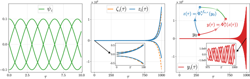
and $\ell_{J}=100$, leading to $\varepsilon=0.1$. The matrix $Q_{s}$ has eigenvalue $1$ with algebraic multiplicity $2$, and $Q_{a}$ has all non-zero off-diagonal entries, fulfilling the conditions of Theorem 4.1. The strong monotonicity condition in Assumption 1-(i) holds since $Q_{s}$ is positive definite. We set $c=1$ and $\delta=100$, with $y(0)=z(0)=(0.1,-0.1,0,0)$ and $\tau(0)=0$ for systems (12)-(13). We also simulate system (14) from $\psi(0)=y(0)$ and the average system (15) from $\zeta(0)=z(0)$. The simulated trajectories are shown in Figure 1, which illustrates three key aspects of our theoretical analysis. The left panel shows the periodic behavior of the linear system (14), where the $\psi$ components exhibit bounded oscillations consistent with the periodic flow predicted by Lemma 4.1. The middle panel validates the averaging analysis by showing how the solution $z(\tau)$ of the pulled-back system (13) closely follows the solution $\zeta(\tau)$ of the averaged system (15) on the time scale $\mathcal{O}(1/\varepsilon)$. Both trajectories display exponential growth. The right panel shows the exponential growth of the solution $y(\tau)$ of the scaled Nesterov’s ODE in (12) confirming the instability predicted by Theorem 4.1.

Figure 2: Comparison of trajectories of $|q(t)-x^{*}|$ under Nesterov’s ODE and the restarting HDS $\mathcal{H}$.

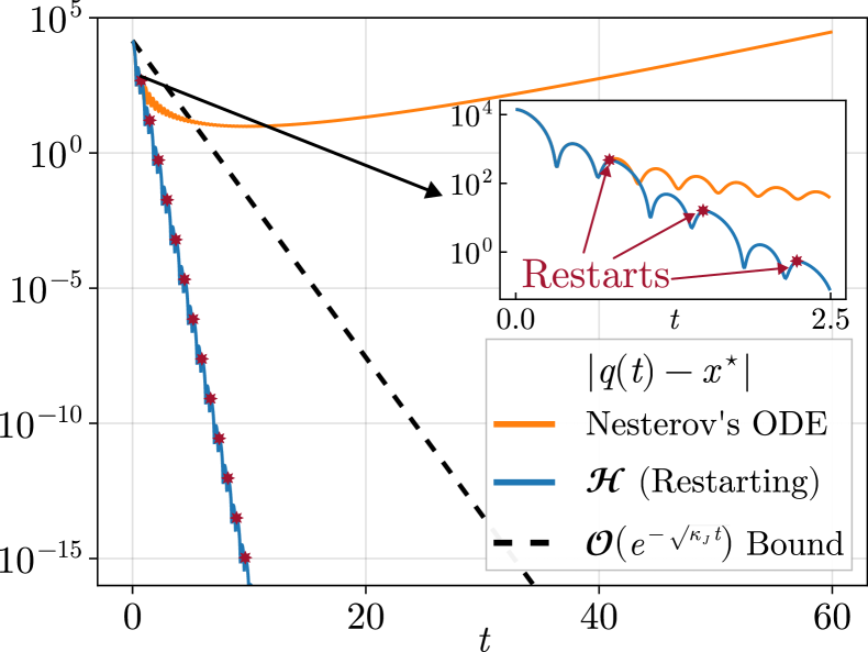
Precluding Instability via Restarting: We simulate the restarting HDS $\mathcal{H}$ using the same vector field $\mathcal{G}(x)=(Q_{s}+Q_{a})x$, which yields $\ell_{K}=5$, $\ell_{J}=100$, and $\kappa_{J}=100$. We set $\eta=1/2$, $T_{0}=0.1$ and $T=T^{\text{opt}}=0.471$, where $T$ satisfies the resetting frequency band condition $T\in(\underline{T},\theta\overline{T})$ introduced in Theorem 5.1. Starting from $\chi(0,0)=(10^{4},-10^{4},10^{4},-10^{4},0.1)$, Figure 2 shows the evolution of $|q(t)-x^{*}|$ for both Nesterov’s ODE and the hybrid mechanism. The red stars indicate the resetting events. The simulations confirm both the uniform global exponential stability property of Theorem 5.1 and the $\mathcal{O}(e^{-\sqrt{\kappa_{J}}t})$ convergence rate established in Corollary 5.1, showing how the hybrid mechanism stabilizes the system while achieving accelerated convergence rates comparable to those of Nesterov’s ODE in the conservative case.

7 Conclusions and Future Directions

In this article, we established two key results regarding Nesterov’s ODE in non-conservative settings. First, we proved that for linear vector fields with nonzero skew-symmetric components, Nesterov’s ODE can exhibit instability even under strong monotonicity conditions. Second, we designed a hybrid dynamical system that recovers stability while achieving convergence rates of $\mathcal{O}(e^{-\sqrt{\kappa_{J}}t})$ through periodic restarting mechanisms, that improve over previous approaches in the literature. Future work will focus on establishing necessary conditions in Assumption 1 and their connection to the contractivity condition of (Ochoa and Poveda, 2024), as well as leveraging Lie bracket expansions of the pullback operator to analyze the instability of Nesterov’s ODE in the case of nonlinear vector fields in the non-conservative setting.

References

- Agračev and Gamkrelidze (1979) Agračev, A.A. and Gamkrelidze, R.V. (1979). The Exponential Representation of Flows and the Chronological Calculus. Mathematics of the USSR-Sbornik, 35(6), 727–785. 10.1070/SM1979v035n06ABEH001623.
- Bullo (2002) Bullo, F. (2002). Averaging and Vibrational Control of Mechanical Systems. SIAM Journal on Control and Optimization, 41(2), 542–562. 10.1137/S0363012999364176.
- Bullo and Lewis (2005) Bullo, F. and Lewis, A.D. (2005). Geometric Control of Mechanical Systems: Modeling, Analysis, and Design for Simple Mechanical Control Systems, volume 49 of Texts in Applied Mathematics. Springer New York, New York, NY. 10.1007/978-1-4899-7276-7.
- Franca et al. (2018) Franca, G., Robinson, D., and Vidal, R. (2018). ADMM and Accelerated ADMM as Continuous Dynamical Systems. In Proceedings of the 35th International Conference on Machine Learning, 1559–1567. PMLR.
- Gaudio et al. (2020) Gaudio, J.E., Annaswamy, A.M., Bolender, M.A., Lavretsky, E., and Gibson, T.E. (2020). A class of high order tuners for adaptive systems. IEEE Control Systems Letters, 5(2), 391–396.
- Gharesifard and Cortés (2014) Gharesifard, B. and Cortés, J. (2014). Distributed Continuous-Time Convex Optimization on Weight-Balanced Digraphs. IEEE Transactions on Automatic Control, 59(3), 781–786. 10.1109/TAC.2013.2278132.
- Glötzl and Richters (2023) Glötzl, E. and Richters, O. (2023). Helmholtz decomposition and potential functions for n-dimensional analytic vector fields. Journal of Mathematical Analysis and Applications, 525(2), 127138. 10.1016/j.jmaa.2023.127138.
- Goebel et al. (2012) Goebel, R., Sanfelice, R.G., and Teel, A.R. (2012). Hybrid Dynamical Systems: Modeling, Stability, and Robustness. Princeton university press, Princeton (N.J.).
- Kim and Fessler (2018) Kim, D. and Fessler, J.A. (2018). Adaptive restart of the optimized gradient method for convex optimization. Journal of Optimization Theory and Applications, 178(1), 240–263.
- Mertikopoulos et al. (2019) Mertikopoulos, P., Lecouat, B., Zenati, H., Foo, C.S., Chandrasekhar, V., and Piliouras, G. (2019). Optimistic Mirror Descent in Saddle-Point Problems: Going the Extra (Gradient) Mile. In ICLR 2019 - 7th International Conference on Learning Representations, 1.
- Morse (1992) Morse, A.S. (1992). High-order parameter tuners for the adaptive control of nonlinear systems. In Robust Control: Proceedings of a workshop held in Tokyo, Japan, June 23–24, 1991, 138–145. Springer.
- Nesterov (1983) Nesterov, Y. (1983). A method for solving the convex programming problem with convergence rate $O(1/k^2)$. Proceedings of the USSR Academy of Sciences.
- Ochoa et al. (2024) Ochoa, D.E., Javed, M.U., Chen, X., and Poveda, J.I. (2024). Decentralized concurrent learning with coordinated momentum and restart. Systems & Control Letters, 193, 105931. 10.1016/j.sysconle.2024.105931.
- Ochoa and Poveda (2024) Ochoa, D.E. and Poveda, J.I. (2024). Momentum-Based Nash Set-Seeking Over Networks via Multitime Scale Hybrid Dynamic Inclusions. IEEE Transactions on Automatic Control, 69(7), 4245–4260. 10.1109/TAC.2023.3321901.
- O’donoghue and Candes (2015) O’donoghue, B. and Candes, E. (2015). Adaptive restart for accelerated gradient schemes. Foundations of computational mathematics, 15, 715–732.
- Poveda and Li (2021) Poveda, J.I. and Li, N. (2021). Robust hybrid zero-order optimization algorithms with acceleration via averaging in time. Automatica, 123, 109361.
- Roulet and d’Aspremont (2017) Roulet, V. and d’Aspremont, A. (2017). Sharpness, restart and acceleration. Advances in Neural Information Processing Systems, 30.
- Sanders et al. (2007) Sanders, J.A., Verhulst, F., and Murdock, J. (2007). Averaging Methods in Nonlinear Dynamical Systems, volume 59 of Applied Mathematical Sciences. Springer New York, New York, NY. 10.1007/978-0-387-48918-6.
- Sarychev (2001) Sarychev, A.V. (2001). Lie- and chronologico-algebraic tools for studying stability of time-varying systems. Systems & Control Letters, 43(1), 59–76. 10.1016/S0167-6911(01)00090-1.
- Shi et al. (2022) Shi, B., Du, S.S., Jordan, M.I., and Su, W.J. (2022). Understanding the acceleration phenomenon via high-resolution differential equations. Mathematical Programming, 195(1), 79–148. 10.1007/s10107-021-01681-8.
- Su et al. (2016) Su, W., Boyd, S., and Candès, E.J. (2016). A Differential Equation for Modeling Nesterov’s Accelerated Gradient Method: Theory and Insights. Journal of Machine Learning Research, 17(153), 1–43.
- Teel et al. (2013) Teel, A.R., Forni, F., and Zaccarian, L. (2013). Lyapunov-Based Sufficient Conditions for Exponential Stability in Hybrid Systems. IEEE Transactions on Automatic Control, 58(6), 1591–1596. 10.1109/TAC.2012.2228039.
- Teel et al. (2019) Teel, A.R., Poveda, J.I., and Le, J. (2019). First-order optimization algorithms with resets and hamiltonian flows. In 2019 IEEE 58th Conference on Decision and Control (CDC), 5838–5843. IEEE.
- Wibisono et al. (2016) Wibisono, A., Wilson, A.C., and Jordan, M.I. (2016). A variational perspective on accelerated methods in optimization. Proceedings of the National Academy of Sciences, 113(47), E7351–E7358.