GANQ: GPU-Adaptive Non-Uniform Quantization for Large Language Models

Abstract

Large Language Models (LLMs) face significant deployment challenges due to their substantial resource requirements. While low-bit quantized weights can reduce memory usage and improve inference efficiency, current hardware lacks native support for mixed-precision General Matrix Multiplication (mpGEMM), resulting in inefficient dequantization-based implementations. Moreover, uniform quantization methods often fail to capture weight distributions adequately, leading to performance degradation. We propose GANQ (GPU-Adaptive Non-Uniform Quantization), a layer-wise post-training non-uniform quantization framework optimized for hardware-efficient lookup table-based mpGEMM. GANQ achieves superior quantization performance by utilizing a training-free, GPU-adaptive optimization algorithm to efficiently reduce layer-wise quantization errors. Extensive experiments demonstrate GANQ’s ability to reduce the perplexity gap from the FP16 baseline compared to state-of-the-art methods for both 3-bit and 4-bit quantization. Furthermore, when deployed on a single NVIDIA RTX 4090 GPU, GANQ’s quantized models achieve up to 2.57$\times$ speedup over the baseline, advancing memory and inference efficiency in LLM deployment.

1 Introduction

Large language models (LLMs) have demonstrated impressive performance across various domains (Brown et al., 2020; Achiam et al., 2023; Touvron et al., 2023a, b; Dubey et al., 2024; Gemini Team et al., 2023; Chowdhery et al., 2023; Zhang et al., 2023; Wang et al., 2023; Arefeen et al., 2024; Li et al., 2024a; Huang et al., 2024). However, their deployment for inference remains challenging due to demanding resource requirements. For example, the LLaMA-3-70B (Dubey et al., 2024) model needs at least 140 GB of GPU memory in FP16, which exceeds current GPU capacities. While larger LLMs often yield better accuracy (Kaplan et al., 2020), these substantial resource demands hinder the practical deployment of LLMs, posing a barrier to their widespread adoption.

Quantization is a promising solution to reduce inference costs for LLMs. For example, 4-bit weight quantization can reduce memory usage for model loading by nearly 75% compared to FP16. In general, quantization techniques are categorized into quantization-aware training (QAT) and post-training quantization (PTQ). QAT integrates quantization into the training process to achieve higher accuracy but is computationally expensive, often requiring extensive samples and significant GPU hours (Liu et al., 2023). This makes QAT impractical for large models. In contrast, PTQ is a cost-effective alternative that applies quantization after training, making it the preferred choice for LLMs (Nagel et al., 2020; Yao et al., 2022; Frantar et al., 2022; Xiao et al., 2023; Dettmers et al., 2023; Kim et al., 2023; Lin et al., 2024; Shao et al., 2024; Ma et al., 2024; Li et al., 2024b). Among PTQ methods, weight-only quantization, which uses low-precision weights while retaining high-precision activations, has become a particularly attractive approach. By reducing memory traffic and alleviating memory-bound bottlenecks, weight-only quantization accelerates inference (Kim et al., 2023). Additionally, compared to weight-activation quantization, it avoids significant accuracy degradation by preserving the precision of activations, ensuring better model performance.

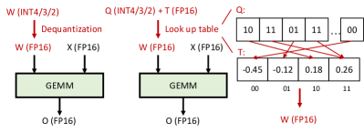
(a) Dequantization-based and LUT-based of mpGEMM.

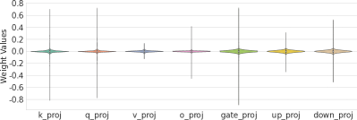
(b) Violin plots of LLaMA-2-7B’s first decoder layer weights.

Figure 1: (a) A comparison of two mpGEMM implementations: a dequantization-based approach (left) versus a LUT-based method (right). (b) Violin plots showing the first decoder layer’s weight distribution in the LLaMA-2-7B model, clearly illustrating their deviation from a uniform distribution.

Despite its promise, weight-only quantization faces two key challenges. First, it shifts the core computation of LLM inference from standard General Matrix Multiplication (GEMM) to mixed-precision GEMM (mpGEMM), where low-precision weights (e.g., INT4/3/2) are multiplied with high-precision activations (e.g., FP16). Current hardware lacks native support for mpGEMM, necessitating dequantization to upscale low-bit weights into supported formats (see the left part of Figure 1(a)). This additional step introduces inefficiencies, particularly in large-batch scenarios, undermining the expected performance gains (Mo et al., 2024). Second, most existing methods rely on uniform quantization $\mathcal{Q}:\mathbb{R}\to[0,2^{N}-1]\cap\mathbb{Z}$ defined as $\mathcal{Q}(x)=\text{clamp}(\lfloor\frac{x}{s}\rceil)+z,0,2^{N}-1)$, where $\lfloor\cdot\rceil$ denotes rounding $N$ is the target bit width, $s$ is the scaling factor, and $z$ is the zero-point (Frantar et al., 2022; Xiao et al., 2023; Dettmers et al., 2023; Lin et al., 2024; Shao et al., 2024; Ma et al., 2024; Li et al., 2024b). However, LLM weight distributions are often highly non-uniform (see Figure 1(b)), making uniform quantization inadequate and resulting in suboptimal representations, particularly due to outliers. Techniques such as introducing learnable scale and zero-point parameters (Shao et al., 2024), applying affine transformations to preprocess weights (Ma et al., 2024), or splitting weights into various components and quantizing those that are easier to process (Dettmers et al., 2023; Li et al., 2024b), have been proposed to mitigate these issues. While these methods improve accuracy, they primarily address challenges within the uniform quantization framework rather than fundamentally enhancing the quantization method itself. Furthermore, they often increase computational complexity during inference due to the extra operations they require.

To address these issues, we propose GANQ (GPU-Adaptive Non-Uniform Quantization), a layer-wise post-training non-uniform quantization framework optimized for lookup table (LUT)-based mpGEMM. In LUT-based mpGEMM (see the right part of Figure 1(a)), complex computations are replaced with simple table lookups, supported by several GPU kernels (Kim et al., 2023; Mo et al., 2024). The primary challenge then becomes how to determine effective low-bit representations for the LUTs. Existing non-uniform quantization methods often rely on heuristic-based approaches, such as manually designed mappings (e.g., power-exponent functions (Yvinec et al., 2023)) or clustering-based methods with heuristic distance metrics (Han et al., 2015; Xu et al., 2018; Kim et al., 2023). While these methods may achieve good results in specific cases, their heuristic nature limits generalization and theoretical grounding. In contrast, GANQ introduces a principled optimization model for layer-wise LUT-based non-uniform quantization, formulated as a mixed-integer quadratic programming problem. This model minimizes the the discrepancy between the outputs of the quantized and original layers, thereby preserving accuracy. To efficiently address this complex model, GANQ utilizes its decomposable structure to divide the original optimization task into multiple independent one-dimensional subproblems, which can be processed in parallel using GPU acceleration to achieve substantial computational efficiency. Besides, GANQ employs an alternating direction optimization framework that capitalizes on the splittable structure of decision variables, effectively reducing quantization error.

In addition, although GANQ is designed as a base quantization method, it is fully compatible with current techniques for handling outliers, such as splitting weights into sparse components (to address outliers) and quantized components (Dettmers et al., 2023; Kim et al., 2023), thereby enabling further performance enhancements.

We evaluate GANQ extensively across various model families and sizes on language modeling tasks. The results show that GANQ consistently outperforms previous methods in quantization performance. Moreover, GANQ is highly resource-efficient and easy to implement. For instance, GANQ processes the LLaMA-2-7B model on a single NVIDIA RTX 4090 GPU in approximately one hour using only 128 samples. Additionally, our deployed models on the NVIDIA RTX 4090 GPU achieve significant latency improvements, with speedups of up to 2.57$\times$ compared to the FP16 baseline. These results highlight the effectiveness of GANQ in both quantization quality and inference efficiency.

2 Related Work

Quantization for LLMs. Quantization reduces the bit-precision of neural networks, resulting in smaller models and faster inference. It has become a key direction for compressing LLMs given their growing size and inference costs. Current quantization methods for LLMs are broadly categorized into QAT (Liu et al., 2023) and PTQ (Nagel et al., 2020; Yao et al., 2022; Frantar et al., 2022; Xiao et al., 2023; Dettmers et al., 2023; Kim et al., 2023; Lin et al., 2024; Shao et al., 2024; Ma et al., 2024; Li et al., 2024b). QAT integrates quantization into the training process, preserving high performance but incurring prohibitive training costs, making it impractical for LLMs. In contrast, PTQ applies quantization to pretrained models, requiring only a small subset of data and modest computational resources, making it particularly appealing for LLMs. PTQ methods can be further classified into wight-only quantization and weight-activation quantization.

Weight-only quantization focuses on compressing model weights into low-bit formats. For example, GPTQ (Frantar et al., 2022) utilizes the optimal brain surgeon framework (Hassibi & Stork, 1992) for quantization and reconstruction. OminiQuant (Shao et al., 2024) introduces learnable parameters to determine quantization factors (e.g., scale and zero-point), while AffineQuant (Ma et al., 2024) extends this idea by incorporating a learnable matrix to preprocess weights before quantization.

Weight-activation quantization compresses both weights and activations, often addressing their quantization jointly. For example, SmoothQuant (Xiao et al., 2023) shifts quantization difficulty from activations to weights using manually designed scaling factors. Similarly, SVDQuant (Li et al., 2024b) applies this approach while further decomposing weights into low-rank and quantized components.

While weight-activation quantization can offer broader compression, studies (Kim et al., 2023; Lin et al., 2024) have shown that LLM inference, especially during generation, is heavily memory-bound, with weight access dominating activation access by orders of magnitude. Consequently, weight-only quantization is more effective for on-device deployment of LLMs. In this work, we focus on weight-only PTQ for its efficiency and suitability for LLMs.

Outlier Mitigation. Due to the widely used uniform quantization mapping and the inherent non-uniform distribution of LLM weights, a key challenge is the presence of outliers. These outliers unnecessarily expand the quantization range (see Figure 1(b)), comprising quantization performance. Recent methods have been proposed to address this issue. For example, SpQR (Dettmers et al., 2023) and SqueezeLLM (Kim et al., 2023) retain outliers in sparse matrices while applying quantization to the remaining weights to mitigate their impact on overall performance. AWQ (Lin et al., 2024) independently quantizes the channel-wise salient weights to improve performance, and SVDQuant (Li et al., 2024b), as mentioned, decomposes weights into low-rank and quantized components. While these methods effectively handle outliers and enhance quantization performance, they often introduce additional computational overhead during inference. For instance, SpQR and SqueezeLLM require both mpGEMM and sparse matrix multiplication, whereas SVDQuant adds an extra low-rank computation branch.

In this work, we propose a direct solution by introducing a non-uniform quantization framework that adapts to the distribution of LLM weights. Furthermore, our method is compatible with these outlier-handling techniques, enabling further performance enhancements when combined.

Non-Uniform Quantization. The non-uniform distribution of weights in LLMs highlights the importance of non-uniform quantization. However, existing non-uniform quantization methods often rely on heuristic-based approaches, limiting their generalization and theoretical grounding. NUPES (Yvinec et al., 2023) replaces uniform quantization with power-exponent functions and employs gradient-based optimization to learn the exponent parameter. Other methods focus on identifying shared weights, thereby forming a codebook, which is suitable for LUT-based mpGEMM. For example, Han et al. (2015) apply $k$-means clustering to minimize the Euclidean distance between weights and centroids in convolutional neural networks (CNNs), while Xu et al. (2018) extend this approach by using a loss-based metric for $k$-means clustering in CNNs. For LLMs, SqueezeLLM (Kim et al., 2023) adapts this idea by leveraging sensitivity-based $k$-means clustering, where the sensitivity metric measures measures the extent to which the model is perturbed after quantization. To mitigate the computational expense of this calculation, SqueezeLLM approximates the required Hessian matrix using the diagonal elements of the Fisher information matrix (Fisher, 1925).

In contrast, we propose a principled optimization model for layer-wise LUT-based non-uniform quantization for LLMs, along with an efficient GPU-adaptive algorithms to solve it.

3 Methodology

3.1 Optimization Model for Non-uniform Quantization

Consider a linear layer with weight matrix $\mathbf{W}\in\mathbb{R}^{m\times n}$ and input activation $\mathbf{X}\in\mathbb{R}^{n\times p}$. As shown in the right part of Figure 1(a), LUT-based quantization aims to compress $\mathbf{W}$ by representing its elements using a codebook. Specifically, the elements of the $i$-th channel in the quantized weight matrix $\mathbf{\widetilde{W}}$ are selected from the codebook $\mathbf{T}_{i}=\{t_{i,0},t_{i,1},\dots,t_{i,2^{N}-1}\}$, where $N$ is the bit-width of the quantization (e.g., 3 or 4 bits). Thus, each element $\mathbf{\widetilde{W}}_{i,j}$ satisfies $\mathbf{\widetilde{W}}_{i,j}\in\mathbf{T}_{i}$.

Table 1: Storage requirements for full-precision (FP16), basic per-channel uniform quantization (4-bit), and per-channel LUT-based non-uniform quantization (4-bit) for weight matrix $\mathbf{W}\in\mathbb{R}^{m\times n}$. Percentages indicate storage usage relative to full-precision representation.

Configuration	Full (FP16)	Basic Uniform (4-bit)	LUT-based (4-bit)
Theory	$2mn$	$0.5mn+4m$	$0.5mn+32m$
$m=n=2048$ (e.g., $\mathbf{W}_{\{k,q,v,o\}}$ in OPT-1.3B)	$100.00\%$	$25.10\%$	$25.78\%$
$m=n=4096$ (e.g., $\mathbf{W}_{\{k,q,v,o\}}$ in LLaMA-2-7B)	$100.00\%$	$25.05\%$	$25.39\%$
$m=n=8192$ (e.g., $\mathbf{W}_{\{k,q,v,o\}}$ in LLaMA-2-70B)	$100.00\%$	$25.02\%$	$25.20\%$

In practice, LUT-based quantization stores two components: a low-bit query matrix $\mathbf{Q}\in\{0,1,\dots 2^{N}-1\}^{m\times n}$, which specifies the indices of values in the codebook, and the codebook itself, $\mathbf{T}\in\mathbb{R}^{m\times 2^{N}}$, which contains the quantized values for each channel. For example, if $\mathbf{Q}_{ij}=0$, then $\mathbf{\widetilde{W}}_{i,j}=t_{i,0}$. Compared to the widely used basic per-channel uniform quantization (Frantar et al., 2022; Xiao et al., 2023), which requires two parameters per channel (i.e., scale and zero-point), this mechanism demands slightly more storage. However, as $\min\{m,n\}\gg 2^{N}$ in practice, the additional storage overhead is negligible. As shown in Table 1, for typical model sizes, the storage usage of LUT-based quantization remains comparable to the basic uniform quantization, differing by less than 0.2%. Moreover, some uniform quantization methods, such as OmniQuant (Shao et al., 2024) and AffineQuant (Ma et al., 2024), also require extra parameters.

To enable effective LUT-based non-uniform quantization, we formulate an optimization model aimed at minimizing the layer-wise output error.:

$$\min_{\mathbf{Q},\mathbf{T}}\|\mathbf{W}\mathbf{X}-\mathbf{\widetilde{W}}\mathbf{X}\|_{F}^{2},\;s.t.\;\mathbf{\widetilde{W}}_{i,j}=\mathbf{T}_{i,\mathbf{Q}_{i,j}},\;\forall i,j,$$ (1)

where $\|\cdot\|_{F}$ denotes the Frobenius norm, and $\mathbf{Q}$ and $\mathbf{T}$ are the decision variables.

Note that the quantized output for each row $(\mathbf{\widetilde{W}}\mathbf{X})_{i,:}$ depends only on its corresponding codebook $\mathbf{T}_{i,:}$ and query vector $\mathbf{Q}_{i,:}$. Consequently, the model in (1) is inherently decomposable across the rows of $\mathbf{W}$. Leveraging this property, the problem can be reformulated into $m$ independent subproblems, which are highly parallelizable and particularly suitable for GPU acceleration. Specifically, this parallelization is achieved by expressing computations in matrix form, which enables efficient matrix-vector and element-wise operations across rows. Furthermore, each subproblem can be expressed as a mixed-integer quadratic programming problem:

$$\min_{\mathbf{S}_{i},\mathbf{T}_{i}}\|\mathbf{W}_{i}\mathbf{X}-\mathbf{T}_{i}\mathbf{S}_{i}\mathbf{X}\|^{2}\;s.t.\;\mathbf{1}^{\top}\mathbf{S}_{i}=\mathbf{1}^{\top},\;\forall i,$$ (2)

where $\mathbf{W}_{i}\in\mathbb{R}^{1\times n}$ is the $i$-th row of $\mathbf{W}$, $\mathbf{T}_{i}\in\mathbb{R}^{1\times 2^{N}}$ is the $i$-th row of $\mathbf{T}$, $\mathbf{S}_{i}\in\{0,1\}^{2^{N}\times n}$ is a column-wise one-hot encoding matrix indicating the mapping of elements from $\mathbf{T}_{i}$, and $\mathbf{1}$ denotes an all-one vector.

The mixed-integer structure of $\mathbf{S}_{i}$ introduces significant combinatorial complexity, and the bilinear interaction between $\mathbf{S}_{i}$ and $\mathbf{T}_{i}$ in the objective further compounds the computational challenge, rendering the problem inherently non-convex and non-smooth. These factors pose serious difficulties for off-the-shelf solvers, especially in large-scale settings with high-dimensional weight matrices and input activations. In response, we develop a specialized, GPU-adaptive approach tailored to navigate this complex search space while scaling to practical problem sizes.

3.2 GPU-Adaptive Non-uniform Quantization Method

To efficiently solve the model in (2) for LUT-based non-uniform quantization, we employ an alternating direction optimization framework. This framework iteratively updates $\mathbf{S}_{i}$ and $\mathbf{T}_{i}$ by decomposing the objective into two subproblems. Each subproblem optimizes one decision variable while keeping the other fixed. The iterative scheme is outlined as follows:

$$\mathbf{S}_{i}^{k+1}\!=\!\operatorname*{argmin}_{\mathbf{S}_{i}}\!\left\{\|\mathbf{W}_{i}\mathbf{X}-\mathbf{T}_{i}^{k}\mathbf{S}_{i}\mathbf{X}\|^{2}\;|\;\mathbf{1}^{\top}\mathbf{S}_{i}\!=\!\mathbf{1}^{\top}\!\right\}\!\!,$$ (3)

$$\mathbf{T}_{i}^{k+1}\!=\!\operatorname*{argmin}_{\mathbf{T}_{i}}\!\left\{\|\mathbf{W}_{i}\mathbf{X}-\mathbf{T}_{i}\mathbf{S}_{i}^{k+1}\mathbf{X}\|^{2}\right\}\!\!.$$ (4)

The $\mathbf{T}_{i}$-subproblem in (4) is an unconstrained quadratic program and admits a closed form solution given by:

$$\mathbf{T}_{i}^{k+1}\!=\!\mathbf{W}_{i}\mathbf{XX}^{\top}\!(\mathbf{S}_{i}^{k+1})^{\top}\!((\mathbf{S}_{i})^{k+1}\mathbf{XX}^{\top}(\mathbf{S}_{i}^{k+1})^{\top})^{\dagger},$$ (5)

where $(\cdot)^{\dagger}$ denotes the Moore-Penrose inverse. Notably, the matrix $(\mathbf{S}_{i})^{k+1}\mathbf{XX}^{\top}(\mathbf{S}_{i}^{k+1})^{\top}$ has dimensions $2^{N}\times 2^{N}$, which is relatively small in practice (e.g., $16\times 16$ under 4-bit quantization), ensuring that the computation remains efficient. Moreover, computing (5) involves only matrix-vector multiplications, making it highly efficient for GPU acceleration. Since the solutions to all $\mathbf{T}_{i}$-subproblems share the same formulation, they can be combined into a single batch computation by stacking all $\mathbf{W}_{i}$ and $\mathbf{T}_{i}$ vectors row-wise and organizing $\mathbf{S}_{i}$ matrices into a tensor. Then, matrix operations can be used to efficiently compute the batch. This approach leverages modern GPUs’ parallel processing capabilities, significantly reducing computational overhead and improving overall efficiency.

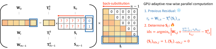
Figure 2: An illustration of the back-substitution framework for determining $\mathbf{S}_{i}$, leveraging the lower triangular structure of $\mathbf{L}$.

The primary challenge lies in the $\mathbf{S}_{i}$-subproblem (3), which is a discrete, non-convex, and non-smooth combinatorial optimization problem. In the case of 4-bit quantization, each element of $\mathbf{S}_{i}$ can assume one of 16 possible values. A brute-force search over all combinations would require $\mathcal{O}(16^{n})$ operations, rendering it computationally prohibitive. Therefore, developing efficient solution techniques is essential for practical applications.

To address the $\mathbf{S}_{i}$-subproblem, we propose an efficient method that leverages the problem’s inherent structure. The objective in (3) can be expanded as:

$$\|\mathbf{W}_{i}\mathbf{X}-\mathbf{T}_{i}^{k}\mathbf{S}_{i}\mathbf{X}\|^{2}$$ (6)

$$= (\mathbf{W}_{i}-\mathbf{T}_{i}^{k}\mathbf{S}_{i})(\mathbf{X}\mathbf{X}^{\top})(\mathbf{W}_{i}-\mathbf{T}_{i}^{k}\mathbf{S}_{i})^{\top}.$$ (7)

Then, consider the Cholesky decomposition of $\mathbf{X}\mathbf{X}^{\top}$:

$$\mathbf{X}\mathbf{X}^{\top}=\mathbf{L}\mathbf{L}^{\top},$$ (8)

where $\mathbf{L}$ is a lower triangle matrix, meaning all its entries above the diagonal are zero.

Remark 3.1.

If $\mathbf{X}\mathbf{X}^{\top}$ is not positive definite, which is rare but can occur in cases like the fc2 layer of OPT models, we can add $\lambda\mathbf{I}$ ($\lambda>0$) to guarantee positive definiteness before Cholesky decomposition. Specifically, for any vector $\mathbf{v}$, $\mathbf{v}^{\top}(\mathbf{X}\mathbf{X}^{\top}+\lambda\mathbf{I})\mathbf{v}=\|\mathbf{X}^{\top}\mathbf{v}\|^{2}+\lambda\|\mathbf{v}\|^{2}>0$.

By combining (7) and (8), we have:

$$(\mathbf{W}_{i}-\mathbf{T}_{i}^{k}\mathbf{S}_{i})(\mathbf{X}\mathbf{X}^{\top})(\mathbf{W}_{i}-\mathbf{T}_{i}^{k}\mathbf{S}_{i})^{\top}$$ (9)

$$= (\mathbf{W}_{i}-\mathbf{T}_{i}^{k}\mathbf{S}_{i})(\mathbf{L}\mathbf{L}^{\top})(\mathbf{W}_{i}-\mathbf{T}_{i}^{k}\mathbf{S}_{i})^{\top}$$ (10)

$$= \|\mathbf{W}_{i}\mathbf{L}-\mathbf{T}_{i}^{k}\mathbf{S}_{i}\mathbf{L}\|^{2}.$$ (11)

Leverage the structure of $\mathbf{L}$, we minimize the upper bound of (11) using a back-substitution approach to efficiently derive a sub-optimal solution to (3). Specifically, there is

$$\|\mathbf{W}_{i}\mathbf{L}-\mathbf{T}_{i}^{k}\mathbf{S}_{i}\mathbf{L}\|^{2}$$ (12)

$$\leq \sum_{j=0}^{n-1}\left(\left(\mathbf{W}_{i}\mathbf{L}\right)_{j}-\left(\mathbf{T}_{i}^{k}\mathbf{S}_{i}\mathbf{L}\right)_{j}\right)^{2}$$ (13)

$$= \sum_{j=0}^{n-1}\!\left(\sum_{u=j}^{n-1}\left({\mathbf{W}_{i,u}}-\mathbf{T}_{i}^{k}\left(\mathbf{S}_{i}\right)_{:,u}\right)\mathbf{L}_{u,j}\right)^{2}.$$ (14)

Following (14), we can solve for $\mathbf{S}_{i}$ from the last column $(j=n-1)$ to the first column ($j=0$), minimizing each of the $n$ squared terms respectively. The $(n-1)$-th column of $\mathbf{L}$ has only one nonzero entry in rows $u\geq n-1$, namely $\mathbf{L}_{n-1,n-1}$. Therefore, for $j=n-1$, the residual involves a single term:

$$\left(\mathbf{W}_{i,n-1}-\mathbf{T}_{i}^{k}\left(\mathbf{S}_{i}\right)_{:,n-1}\right)\mathbf{L}_{n-1,n-1}.$$ (15)

Minimizing with respect to $(\mathbf{S}_{i})_{:,n-1}$ gives that it should select an element from $\mathbf{T}_{i}^{k}$ that satisfies

$$\text{idx}=\operatorname*{argmin}_{s}\left|\mathbf{W}_{i,n-1}-\mathbf{T}^{k}_{i,s}\right|.$$ (16)

Then, we set $(\mathbf{S}_{i})_{\text{idx},n-1}=1$ and all other elements in this column to 0.

Once $(\mathbf{S}_{i})_{:,n-1}$ is determined, the process moves to the $(n-2)$-th column. The residual becomes

$$\left(\mathbf{W}_{i,n-2}-\mathbf{T}_{i}^{k}\left(\mathbf{S}_{i}\right)_{:,n-2}\right)\mathbf{L}_{n-2,n-2}$$ (17)

$$+ \left(\mathbf{W}_{i,n-1}-\mathbf{T}_{i}^{k}\left(\mathbf{S}_{i}\right)_{:,n-1}\right)\mathbf{L}_{n-1,n-2},$$ (18)

where (18) is a constant value given $\left(\mathbf{S}_{i}\right)_{:,n-1}$. In the following steps, we refer to $\mathbf{W}_{i,n-1}-\mathbf{T}_{i}^{k}\left(\mathbf{S}_{i}\right)_{:,n-1}$ as $r_{n-1}$. Then, we solve for $(\mathbf{S}_{i})_{:,n-2}$ by minimizing the square of (17)–(18):

$$\text{idx}=\operatorname*{argmin}_{s}\left|\mathbf{W}_{i,n-2}+\frac{r_{n-1}\mathbf{L}_{n-1,n-2}}{\mathbf{L}_{n-2,n-2}}-\mathbf{T}^{k}_{i,s}\right|,$$ (19)

and we set $(\mathbf{S}_{i})_{\text{idx},n-2}=1$ and the rest of $(\mathbf{S}_{i})_{:,n-2}=0$.

This back-substitution process continues for $j=n-3,\dots,0$. At each step the element of $(\mathbf{S}_{i})_{\text{idx},j}$ set to 1 is determined as

$$\text{idx}=\operatorname*{argmin}_{s}\left|\mathbf{W}_{i,j}+\frac{1}{\mathbf{L}_{j,j}}\sum_{u=j+1}^{n-1}r_{u}\mathbf{L}_{u,j}-\mathbf{T}^{k}_{i,s}\right|.$$ (20)

where $r_{u}=\mathbf{W}_{i,u}-\mathbf{T}_{i}^{k}\left(\mathbf{S}_{i}\right)_{:,u}$.

Figure 2 illustrates the back-substitution framework for efficiently determining $\mathbf{S}_{i}$. Since the solution processes for $\mathbf{S}_{i},i=0,1,\dots,m-1$ are independent, similar to the batch solving of $\mathbf{T}_{i}$-subproblems described earlier, we can stack all $\mathbf{W}_{i}$ and $\mathbf{T}_{i}$ vectors row-wise and organize the $\mathbf{S}_{i}$ matrices into a tensor. This allows the back-substitution process to be performed for the entire problem using matrix operations, leveraging modern GPUs’ parallel processing capabilities to enhance overall efficiency.

Algorithm 1 GANQ: GPU-Adaptive Layer-Wise LUT-Based Non-Uniform Quantization

 Input: $\mathbf{W}\!\!\in\!\!\mathbb{R}^{m\times n}$, $\mathbf{X}\!\!\in\!\!\mathbb{R}^{n\times p}$, initial codebook $\mathbf{T}^{0}\!\!\in\!\!\mathbb{R}^{m\times 2^{N}}$, number of iterations $K$

 Output: Updated $\mathbf{T}^{K}$ and query matrix $\mathbf{Q}^{K}\!\!\in\!\!\{0,2^{N}\!-\!1\}^{m\times n}$

 Initialize $\mathbf{S}^{0}=\mathbf{0}^{m\times 2^{N}\times n}$ # tensor format

 Compute $\mathbf{H}=\mathbf{XX}^{\top}$

 Compute $\mathbf{L}=\text{Cholesky}(\mathbf{H})$ # Cholesky decomposition

 for $k\leftarrow 0$ to $K-1$ do

  Initialize $\mathbf{r}=\mathbf{0}^{m\times 1}$ # previous residual vector

  for $j\leftarrow n-1$ to $0$ do

  $\textbf{idx}=\operatorname*{argmin}_{\mathbf{s}}\left|\mathbf{W}_{:,j}+\frac{\mathbf{r}}{\mathbf{L}_{j,j}}-\mathbf{T}^{k}_{:,\mathbf{s}}\right|$# row-wise

  $\mathbf{Q}^{k+1}_{:,j}=\textbf{idx}$

  Update $\mathbf{S}^{k+1}_{:,:,j}$ using idx # one-hot encoding

  $\mathbf{r}=(\mathbf{W}_{:,j:}-\mathbf{T}^{k}\mathbf{S}_{:,:,j:}^{k+1})\mathbf{L}_{j:,j}$ # update residual

  end for

  $\mathbf{T}^{k+1}\!\!=\!\!\mathbf{W}\mathbf{H}(\mathbf{S}^{k+1})^{\top}\!((\mathbf{S}^{k+1})\mathbf{H}^{\top}\!(\mathbf{S}^{k+1})^{\top}\!)^{\dagger}$ # batch update

 end for

 Return $\mathbf{T}^{K},\mathbf{Q}^{K}$

Finally, the full pseudocode of GANQ for layer-wise LUT-based non-uniform quantization is presented in Algorithm 1.

3.3 Compatibility with Outlier-Handling Techniques

GANQ provides a foundational framework for LUT-based non-uniform quantization and is inherently compatible with existing techniques for handling outliers in weight matrices. Among these techniques, a widely adopted approach involves splitting the weight matrix into a sparse matrix for outliers and a quantized matrix for the remaining weights. For example, SpQR (Dettmers et al., 2023) and SqueezeLLM (Kim et al., 2023) extract outliers into a separate sparse matrix to mitigate their impact on the quantization process.

In our framework, the weight matrix $\mathbf{W}$ can similarly be decomposed into a sparse component $\mathbf{W}_{\text{sparse}}$, containing extracted outliers, and a dense component $\mathbf{W}_{\text{dense}}$, processed through GANQ. The method for extracting outliers is detailed in Appendix A. This decomposition reduces quantization range, thereby enhancing the quantization performance.

4 Experiments

4.1 Settings

Quantization. We evaluate GANQ on weight-only non-uniform quantization. The default configuration employs INT4/3 per-channel weight quantization.

Models. We comprehensively evaluate GANQ on a range of models, including OPT (Zhang et al., 2022), LLaMA (Touvron et al., 2023a), LLaMA-2 (Touvron et al., 2023b), and LLaMA-3 (Meta AI, 2024) families. Specifically, we assess its performance across OPT-125M, OPT-350M, OPT-1.3B, OPT-2.7B, OPT-6.7B, LLaMA-7B, LLaMA-2-7B, and LLaMA-3-8B models.

Evaluation. Following prior work (Frantar et al., 2022; Shao et al., 2024; Ma et al., 2024; Kim et al., 2023), we evaluate the quantized models by reporting perplexity on language generation tasks, specifically using the WikiText-2 (Merity et al., 2016), C4 (Raffel et al., 2020), and PTB (Marcus et al., 1994) datasets. Additionally, we assess accuracy on zero-shot tasks, including ARC Easy, ARC Challenge (Clark et al., 2018), WinoGrande (Sakaguchi et al., 2021), BoolQ (Clark et al., 2019), RTE (Wang et al., 2018), and HellaSwag (Zellers et al., 2019), facilitated by the LM Harness library (Gao et al., 2021).

Baselines. For basic weight-only quantization, we compare GANQ with standard round-to-nearest uniform quantization (RTN), GPTQ (Frantar et al., 2022), and OminiQuant (Shao et al., 2024). For weight-only quantization with outlier handling, we compare with GPTQ, OminiQuant, and AWQ (Lin et al., 2024), each using a group size of 128, as well as SqueezeLLM (Kim et al., 2023).

Setup. We implement GANQ using PyTorch (Paszke et al., 2019) and utilize the HuggingFace Transformers library (Wolf, 2019) for model and dataset management. All experiments are conducted on a single NVIDIA RTX 4090 GPU. For calibration data, we follow the methodology outlined in previous works (Frantar et al., 2022; Shao et al., 2024; Kim et al., 2023). Specifically, we use 32 sequences for OPT models and 128 sequences for LLaMA models. Each sequence consists of 2048 tokens, sampled from the first shard of the C4 dataset.

Latency Profiling. Following prior works and associated quantized model inference kernels (GPTQ-for-LLaMa, 2023; Kim et al., 2023), we evaluate latency and peak memory usage while generating 1024 tokens on a single NVIDIA RTX 4090 GPU using the Torch CUDA profiler.

4.2 Main Results

Table 2: WikiText2 perplexity ($\downarrow$) of quantized models under 4-bit and 3-bit. GANQ outperforms state-of-the-art methods.

Method	Bit-width	OPT					LLaMA
		125M	350M	1.3B	2.7B	6.7B	7B	2-7B	3-8B
Full	16	27.66	22.00	14.63	12.47	10.86	5.68	5.47	6.13
RTN	4	37.11	25.94	48.18	16.73	12.14	6.29	6.12	8.53
GPTQ	4	31.08	23.99	15.60	12.88	11.45	6.95	6.08	2.4e2
OminiQuant	4	30.98	23.34	15.25	12.84	11.25	5.92	5.88	–
GANQ	4	28.58	23.04	14.94	12.33	10.70	5.83	5.65	6.61
RTN	3	1.3e3	64.56	1.3e4	1.3e4	5.8e3	25.54	5.4e2	2.2e3
GPTQ	3	52.48	34.47	21.60	16.95	15.11	16.65	9.46	1.4e2
OminiQuant	3	42.43	29.64	18.22	19.47	13.47	6.79	7.08	–
GANQ	3	35.98	29.42	17.05	14.10	11.39	6.33	6.25	8.83

Table 3: Accuracies (%, $\uparrow$) of the quantized LLaMA-2-7B model on 6 zero-shot tasks under 4-bit and 3-bit quantization.

Method	Bit-width	HellaSwag	BoolQ	RTE	WinoGrande	Arc-e	Arc-c	Mean
Full	16	57.12	77.68	63.18	69.06	76.35	43.43	64.47
RTN	4	55.59	73.61	59.57	68.43	74.03	41.30	62.09
GPTQ	4	55.66	74.43	57.76	57.72	75.25	42.32	60.52
OminiQuant	4	55.66	75.69	63.90	68.19	74.33	39.85	62.94
GANQ	4	56.10	77.31	65.70	68.75	74.96	42.58	64.23
RTN	3	30.93	42.54	52.71	52.17	34.76	21.33	39.07
GPTQ	3	47.55	67.03	55.60	59.75	64.60	33.11	54.61
OminiQuant	3	52.58	72.11	57.40	64.72	68.73	36.43	58.66
GANQ	3	53.85	75.02	62.82	67.48	73.36	40.78	62.22

Weight-only Quantization. The results in Table 2 present the WikiText2 perplexity of various quantized models under 4-bit and 3-bit configurations across different model sizes (with additional perplexity results on the C4 and PTB datasets in Appendix B). As shown, GANQ consistently outperforms baseline methods such as RTN, GPTQ, and OminiQuant across all configurations. For 4-bit quantization, GANQ achieves the lowest perplexity across both OPT and LLaMA models, with notable improvements. Remarkably, on OPT-2.7B, GANQ’s perplexity (12.33) even outperforms the full-precision FP16 model (12.47). GANQ also demonstrates strong performance with 3-bit quantization, maintaining competitive perplexity reductions across model sizes. For example, on OPT-6.7B, GANQ’s perplexity is 11.39, compared to 15.11 for GPTQ and 13.47 for OminiQuant. These results underscore GANQ’s effectiveness in both 4-bit and 3-bit quantization, achieving substantial perplexity reductions across various model scales. The “–” in Table 2 indicates that OmniQuant cannot quantize LLaMA-3-8B on a single RTX 4090 GPU due to memory constraints or the unavailability of the pre-quantized model.

The results in Table 3 show the zero-shot performance of the quantized LLaMA-2-7B model across six tasks under 4-bit and 3-bit quantization. GANQ outperforms baseline methods such as RTN, GPTQ, and OmniQuant in both bit-width configurations. With 4-bit quantization, GANQ achieves an average accuracy of 64.23%, which is comparable to the full-precision model (64.47%). For 3-bit quantization, GANQ maintains strong performance with an average accuracy of 62.22%, significantly surpassing other baseline methods. These results demonstrate GANQ’s ability to preserve high task performance, even under aggressive quantization.

Weight-only Quantization with Outlier Handling. To mitigate outlier impact, methods like RTN, GPTQ, AWQ, and OminiQuant divide per-channel distributions into smaller blocks (typically of size 128). SqueezeLLM retains a small percentage of outliers (e.g., 0.5%) and a fixed number of full rows (default: 10). GANQ can integrate seamlessly with SqueezeLLM’s outlier handling mechanism. We evaluate this integration through experiments. Due to memory constraints, OmniQuant cannot quantize LLaMA-3-8B, and SqueezeLLM is limited to models up to 2.7B. We use results directly from their paper for these cases if available. Additionally, SqueezeLLM’s current code does not support OPT-350M. For GANQ, we retain 0.5% outliers for all OPT models and LLaMA-3-8B. Additionally, we retain 10 full rows for LLaMA-7B and LLaMA-2-7B to ensure a fair comparison with SqueezeLLM

As shown in Table 4, GANQ^⋆ (indicating GANQ integrated with outlier handling) outperforms other baselines. Furthermore, when retaining only 0.5% of outliers for LLaMA-7B and LLaMA-2-7B, we observe the following results: LLaMA-7B (5.78 for 4-bit, 6.20 for 3-bit), LLaMA-2-7B (5.60 for 4-bit, 6.10 for 3-bit), which still outperform all other methods, except for SqueezeLLM.

Table 4: WikiText2 perplexity ($\downarrow$) of quantized models under 4-bit and 3-bit. GANQ outperforms state-of-the-art methods.

Method	Bit-width	OPT					LLaMA
		125M	350M	1.3B	2.7B	6.7B	7B	2-7B	3-8B
Full	16	27.66	22.00	14.63	12.47	10.86	5.68	5.47	6.13
RTN (g128)	4	30.49	24.51	15.29	12.80	11.15	5.96	5.72	6.73
GPTQ (g128)	4	29.78	23.40	14.91	12.50	10.99	6.40	5.65	8.97
AWQ (g128)	4	29.09	1.3e4	14.93	12.70	10.96	5.78	5.60	6.53
OminiQuant (g128)	4	29.57	22.85	14.88	12.66	11.04	5.79	5.62	–
SqueezeLLM	4	28.51	–	14.83	12.60	10.92	5.77	5.57	–
GANQ⋆	4	28.16	22.84	14.53	12.19	10.69	5.76	5.57	6.50
RTN (g128)	3	50.61	36.33	1.2e2	2.6e2	22.87	7.01	6.66	12.07
GPTQ (g128)	3	37.93	28.21	16.33	13.57	11.30	8.68	6.43	19.87
AWQ (g128)	3	35.75	1.7e4	16.31	13.56	11.39	6.35	6.24	8.22
OminiQuant (g128)	3	35.61	27.65	16.16	13.28	11.23	6.30	6.23	–
SqueezeLLM	3	32.59	–	15.76	13.43	11.31	6.13	5.96	–
GANQ⋆	3	32.35	26.84	15.52	13.11	11.13	6.08	5.93	7.46

Table 5: Comparison CUDA time (s), speedup ($\uparrow$), and peak memory (GB) ($\downarrow$) for uniform and LUT-based quantization methods on OPT-6.7B and LLaMA-7B models.

Method	Bit-width	OPT-6.7B			LLaMA-7B
		CUDA time	Speedup ($\uparrow$)	Peak Memory ($\downarrow$)	CUDA time	Speedup ($\uparrow$)	Peak Memory ($\downarrow$)
Full	16	16.76	1.0	12.91	17.86	1.00	13.06
GPTQ	4	44.19	0.38	4.30	50.92	0.35	4.07
GPTQ (g128)	4	48.37	0.35	4.42	54.73	0.33	4.18
GANQ	4	7.47	2.24	4.88	8.46	2.11	4.14
GANQ	3	6.51	2.57	4.10	7.48	2.39	3.30

4.3 Profiling

We present the CUDA time, speedup, and peak GPU memory usage of GANQ in Table 5, measured on a single NVIDIA RTX 4090 GPU across different configurations when generating 1024 tokens. GANQ achieves up to a 2.57$\times$ speedup compared to the FP16 baseline, with peak memory usage reduced to 4.10 GB for OPT-6.7B and 3.30 GB for LLaMA-7B at 3-bit quantization. Furthermore, the lack of native support for mpGEMM in uniform quantization methods (e.g., GPTQ) significantly slows down the overall inference process. In contrast, GANQ incurs only a slight increase in memory usage compared to uniform quantization, underscoring that the overhead of LUT-based dequantization is minimal, especially when weighed against the significant improvements in perplexity and latency. Note that the GPTQ-for-LLaMA (GPTQ-for-LLaMa, 2023) package does not currently support 3-bit inference, so no 3-bit results are reported for GPTQ. We expect similar performance to the 4-bit quantization results.

4.4 Quantization Cost

Among the evaluated methods, RTN, GPTQ, and AWQ are the most efficient in GPU memory usage and quantization time, due to their layer-wise heuristic approach. However, they trade off model performance. In contrast, OmniQuant and SqueezeLLM require gradient information, leading to higher memory demands. OmniQuant can quantize 7B models on a single RTX 4090 GPU but fails for 8B models and takes over 3 hours for 7B quantization. SqueezeLLM, which requires global gradients, can only quantize models up to 2.7B. GANQ leverages GPU-adaptive, parallel row-wise computation to quantize 7B models in approximately 1 hour for $K=10$. Considering both model performance and quantization cost, GANQ is an effective solution.

5 Conclusion

In this work, we introduce GANQ, a GPU-adaptive non-uniform quantization framework for efficient deployment and inference of LLMs. GANQ introduces a principled optimization model for layer-wise LUT-based quantization, formulated as a mixed-integer quadratic programming problem, and solves it efficiently using a GPU-adaptive alternating direction optimization algorithm. Extensive experiments demonstrate that GANQ reduces perplexity compared to state-of-the-art methods in 3-bit and 4-bit quantization settings, while preserving high accuracy. Additionally, GANQ achieves up to 2.57$\times$ speedup over FP16 baselines on a single NVIDIA RTX 4090 GPU, showcasing its substantial improvements in both memory usage and inference efficiency. GANQ is highly resource-efficient, easy to implement, and compatible with existing techniques for handling outliers, making it a highly flexible solution for large-scale LLM deployment. These results highlight GANQ’s potential to enable practical and efficient deployment of high-performance LLMs across a wide range of hardware configurations.

Appendix A Outlier Extraction Method

In this section, we describe the method we implemented to extract outliers from the matrix $\mathbf{W}$. This method decomposes $\mathbf{W}$ into two components: a sparse component $\mathbf{W}_{\text{sparse}}$, which contains the extracted outliers, and a dense component $\mathbf{W}_{\text{dense}}$, which consists of the remaining non-outlier values. We then perform quantization on $\mathbf{W}_{\text{dense}}$ to enhance quantization performance.

Algorithm 2 Outlier Extraction and Weight Decomposition

 Input: Weight matrix $\mathbf{W}\in\mathbb{R}^{m\times n}$, outlier extraction ratio $0<r<1$

 Output: Sparse component $\mathbf{W}_{\text{sparse}}$, Dense component $\mathbf{W}_{\text{dense}}$

 $p\leftarrow 1-0.5\times r$ # compute tail percentile

 $\mathbf{M}\leftarrow\mathbf{0}$ # initialize outlier mask $\mathbf{M}$ with zeros

 $\text{upper}\leftarrow\lfloor n\times p\rfloor$

 $\mathbf{W}_{\text{sorted}}\leftarrow\text{sort}(\mathbf{W}[:])$# row-wise sorting

 $\mathbf{c}_{\text{upper}}\leftarrow\mathbf{W}_{\text{sorted}}[:,\text{upper}]$ # upper cutoff values

 $\text{lower}\leftarrow\lceil n\times(1-p)\rceil$

 $\mathbf{c}_{\text{lower}}\leftarrow\mathbf{W}_{\text{sorted}}[:,\text{lower}]$ # lower cutoff values

 $\mathbf{O}\leftarrow(\mathbf{W}\geq\mathbf{c}_{\text{upper}})\vee(\mathbf{W}\leq\mathbf{c}_{\text{lower}})$ # identify outliers

 $\mathbf{M}[\mathbf{O}]\leftarrow 1$ # mark outliers in the mask

 $\mathbf{W}_{\text{sparse}}\leftarrow\mathbf{W}\circ\mathbf{M}$ # extract outliers

 $\mathbf{W}_{\text{dense}}\leftarrow\mathbf{W}-\mathbf{W}_{\text{sparse}}$ # extract non-outliers

 Return $\mathbf{W}_{\text{sparse}},\mathbf{W}_{\text{dense}}$

The pseudocode is shown in Algorithm 2. This decomposition is achieved through a row-wise outlier extraction process based on an extraction ratio $r$, where $0<r<1$ (e.g., $0.5\%$). The process begins by computing a tail percentile $p=1-0.5\times r$, which determines the boundaries for identifying outliers in each row symmetrically. For each row of the weight matrix, the algorithm sorts the values in ascending order and computes the upper and lower cutoff values corresponding to the percentiles $p$ and $1-p$. These cutoff values define the outliers, which are those values that fall either above the upper percentile or below the lower percentile. An outlier mask $\mathbf{M}$ is then created, where values that are identified as outliers are marked with 1, and non-outliers are marked with 0. The sparse component $\mathbf{W}_{\text{sparse}}$ is obtained by multiplying the weight matrix $\mathbf{W}$ element-wise with the outlier mask, while the dense component $\mathbf{W}_{\text{dense}}$ is obtained by subtracting the sparse component from the original matrix.

Appendix B Additional Results

Table 6: C4 perplexity ($\downarrow$) of quantized models under 4-bit and 3-bit. GANQ outperforms state-of-the-art methods.

Method	Bit-width	OPT					LLaMA
		125M	350M	1.3B	2.7B	6.7B	7B	2-7B	3-8B
Full	16	26.56	22.59	16.07	14.34	12.71	7.34	7.26	9.45
RTN	4	33.89	26.21	27.49	18.83	14.37	8.12	8.16	13.35
GPTQ	4	29.08	24.64	17.00	14.99	13.18	8.83	7.87	51.33
OminiQuant	4	28.76	23.85	16.85	14.93	13.10	7.66	7.77	–
GANQ	4	27.72	23.47	16.54	14.71	12.96	7.52	7.47	10.23
RTN	3	8.3e2	55.15	6.5e3	1.0e4	5.0e3	20.78	5.3e2	5.7e2
GPTQ	3	42.14	30.90	21.52	18.24	17.00	22.28	11.67	70.53
OminiQuant	3	36.37	28.82	19.61	19.10	15.51	8.75	9.38	–
GANQ	3	33.59	29.46	18.46	16.43	13.68	8.20	8.20	12.88

The results in Table 6 present the C4 perplexity of various quantized models under 4-bit and 3-bit configurations across different model sizes. As shown, GANQ outperforms baseline methods such as RTN, GPTQ, and OminiQuant across all configurations. For 4-bit quantization, GANQ achieves the lowest perplexity across both OPT and LLaMA models, with notable improvements. GANQ also demonstrates strong performance with 3-bit quantization, maintaining competitive perplexity reductions across model sizes. On OPT-6.7B, GANQ’s perplexity is 13.68, compared to 17.00 for GPTQ and 15.51 for OminiQuant. These results highlight GANQ’s effectiveness in both 4-bit and 3-bit quantization, achieving substantial perplexity reductions across a wide range of model scales. The symbol ’–’ in Table 6 indicates that OmniQuant cannot quantize LLaMA-3-8B on a single RTX 4090 GPU due to memory constraints, or the quantized model is unavailable in their model zoo.

Table 7: PTB perplexity ($\downarrow$) of quantized models under 4-bit and 3-bit. GANQ outperforms state-of-the-art methods.

Method	Bit-width	OPT
		125M	350M	1.3B	2.7B	6.7B
Full	16	38.99	31.07	20.29	17.97	15.77
RTN	4	53.88	36.79	75.40	32.40	18.86
GPTQ	4	45.45	34.33	22.04	19.19	16.58
OminiQuant	4	42.53	33.80	21.79	19.00	16.18
GANQ	4	40.75	33.21	21.06	18.73	15.95
RTN	3	1.4e3	87.20	1.5e3	1.2e4	5.4e3
GPTQ	3	72.91	47.17	31.94	25.63	21.63
OminiQuant	3	59.56	42.65	26.87	29.82	21.52
GANQ	3	55.67	44.58	24.27	21.28	16.91

The results in Table 7 present the PTB perplexity of various quantized models under 4-bit and 3-bit configurations across different model sizes. As shown, GANQ outperforms baseline methods such as RTN, GPTQ, and OminiQuant across all configurations. For 4-bit quantization, GANQ achieves the lowest perplexity across OPT models with notable improvements. GANQ also demonstrates strong performance with 3-bit quantization, maintaining competitive perplexity reductions across model sizes. On OPT-6.7B, GANQ’s perplexity is 16.91, compared to 21.63 for GPTQ and 21.52 for OminiQuant. These results highlight GANQ’s effectiveness in both 4-bit and 3-bit quantization, achieving substantial perplexity reductions across a range of model sizes.

LLaMA-7B and LLaMA-2-7B perform similarly to the much smaller OPT-125M model in full-precision FP16 configuration on the PTB dataset. Specifically, the FP16 versions of LLaMA-7B (41.15) and LLaMA-2-7B (37.91) do not achieve significantly better perplexity than the OPT-125M model (38.99), highlighting the relative inefficiency of LLaMA models on this dataset. Therefore, we focus on reporting results for OPT models, which demonstrate stronger performance in this context.

References

- Achiam et al. (2023) Achiam, J., Adler, S., Agarwal, S., Ahmad, L., Akkaya, I., Aleman, F. L., Almeida, D., Altenschmidt, J., Altman, S., Anadkat, S., et al. Gpt-4 technical report. arXiv preprint arXiv:2303.08774, 2023.
- Arefeen et al. (2024) Arefeen, M. A., Debnath, B., and Chakradhar, S. Leancontext: Cost-efficient domain-specific question answering using llms. Natural Language Processing Journal, 7:100065, 2024.
- Brown et al. (2020) Brown, T., Mann, B., Ryder, N., Subbiah, M., Kaplan, J. D., Dhariwal, P., Neelakantan, A., Shyam, P., Sastry, G., Askell, A., et al. Language models are few-shot learners. Advances in Neural Information Processing Systems, 33:1877–1901, 2020.
- Chowdhery et al. (2023) Chowdhery, A., Narang, S., Devlin, J., Bosma, M., Mishra, G., Roberts, A., Barham, P., Chung, H. W., Sutton, C., Gehrmann, S., et al. Palm: Scaling language modeling with pathways. Journal of Machine Learning Research, 24(240):1–113, 2023.
- Clark et al. (2019) Clark, C., Lee, K., Chang, M.-W., Kwiatkowski, T., Collins, M., and Toutanova, K. Boolq: Exploring the surprising difficulty of natural yes/no questions. arXiv preprint arXiv:1905.10044, 2019.
- Clark et al. (2018) Clark, P., Cowhey, I., Etzioni, O., Khot, T., Sabharwal, A., Schoenick, C., and Tafjord, O. Think you have solved question answering? try arc, the ai2 reasoning challenge. arXiv preprint arXiv:1803.05457, 2018.
- Dettmers et al. (2023) Dettmers, T., Svirschevski, R., Egiazarian, V., Kuznedelev, D., Frantar, E., Ashkboos, S., Borzunov, A., Hoefler, T., and Alistarh, D. Spqr: A sparse-quantized representation for near-lossless llm weight compression. arXiv preprint arXiv:2306.03078, 2023.
- Dubey et al. (2024) Dubey, A., Jauhri, A., Pandey, A., Kadian, A., Al-Dahle, A., Letman, A., Mathur, A., Schelten, A., Yang, A., Fan, A., et al. The llama 3 herd of models. arXiv preprint arXiv:2407.21783, 2024.
- Fisher (1925) Fisher, R. A. Theory of statistical estimation. In Mathematical proceedings of the Cambridge philosophical society, pp. 700–725. Cambridge University Press, 1925.
- Frantar et al. (2022) Frantar, E., Ashkboos, S., Hoefler, T., and Alistarh, D. Gptq: Accurate post-training quantization for generative pre-trained transformers. arXiv preprint arXiv:2210.17323, 2022.
- Gao et al. (2021) Gao, L., Tow, J., Biderman, S., Black, S., DiPofi, A., Foster, C., Golding, L., Hsu, J., McDonell, K., Muennighoff, N., et al. A framework for few-shot language model evaluation. Version v0. 0.1. Sept, 10:8–9, 2021.
- Gemini Team et al. (2023) Gemini Team, Anil, R., Borgeaud, S., Wu, Y., Alayrac, J.-B., Yu, J., Soricut, R., Schalkwyk, J., Dai, A. M., Hauth, A., et al. Gemini: a family of highly capable multimodal models. arXiv preprint arXiv:2312.11805, 2023.
- GPTQ-for-LLaMa (2023) GPTQ-for-LLaMa. Gptq-for-llama, 2023. URL https://github.com/qwopqwop200/GPTQ-for-LLaMa/tree/triton.
- Han et al. (2015) Han, S., Mao, H., and Dally, W. J. Deep compression: Compressing deep neural networks with pruning, trained quantization and huffman coding. arXiv preprint arXiv:1510.00149, 2015.
- Hassibi & Stork (1992) Hassibi, B. and Stork, D. Second order derivatives for network pruning: Optimal brain surgeon. Advances in neural information processing systems, 5, 1992.
- Huang et al. (2024) Huang, L., Li, Z., Sima, C., Wang, W., Wang, J., Qiao, Y., and Li, H. Leveraging vision-centric multi-modal expertise for 3d object detection. Advances in Neural Information Processing Systems, 36, 2024.
- Kaplan et al. (2020) Kaplan, J., McCandlish, S., Henighan, T., Brown, T. B., Chess, B., Child, R., Gray, S., Radford, A., Wu, J., and Amodei, D. Scaling laws for neural language models. arXiv preprint arXiv:2001.08361, 2020.
- Kim et al. (2023) Kim, S., Hooper, C., Gholami, A., Dong, Z., Li, X., Shen, S., Mahoney, M. W., and Keutzer, K. Squeezellm: Dense-and-sparse quantization. arXiv preprint arXiv:2306.07629, 2023.
- Li et al. (2024a) Li, J., Tang, T., Zhao, W. X., Nie, J.-Y., and Wen, J.-R. Pre-trained language models for text generation: A survey. ACM Computing Surveys, 56(9):1–39, 2024a.
- Li et al. (2024b) Li, M., Lin, Y., Zhang, Z., Cai, T., Li, X., Guo, J., Xie, E., Meng, C., Zhu, J.-Y., and Han, S. Svdqunat: Absorbing outliers by low-rank components for 4-bit diffusion models. arXiv preprint arXiv:2411.05007, 2024b.
- Lin et al. (2024) Lin, J., Tang, J., Tang, H., Yang, S., Chen, W.-M., Wang, W.-C., Xiao, G., Dang, X., Gan, C., and Han, S. Awq: Activation-aware weight quantization for on-device llm compression and acceleration. Proceedings of Machine Learning and Systems, 6:87–100, 2024.
- Liu et al. (2023) Liu, Z., Oguz, B., Zhao, C., Chang, E., Stock, P., Mehdad, Y., Shi, Y., Krishnamoorthi, R., and Chandra, V. Llm-qat: Data-free quantization aware training for large language models. arXiv preprint arXiv:2305.17888, 2023.
- Ma et al. (2024) Ma, Y., Li, H., Zheng, X., Ling, F., Xiao, X., Wang, R., Wen, S., Chao, F., and Ji, R. Affinequant: Affine transformation quantization for large language models. In The Twelfth International Conference on Learning Representations, 2024.
- Marcus et al. (1994) Marcus, M., Kim, G., Marcinkiewicz, M. A., MacIntyre, R., Bies, A., Ferguson, M., Katz, K., and Schasberger, B. The penn treebank: Annotating predicate argument structure. In Human Language Technology: Proceedings of a Workshop held at Plainsboro, New Jersey, March 8-11, 1994, 1994.
- Merity et al. (2016) Merity, S., Xiong, C., Bradbury, J., and Socher, R. Pointer sentinel mixture models. arXiv preprint arXiv:1609.07843, 2016.
- Meta AI (2024) Meta AI. Llama-3: Meta ai’s latest language model. https://ai.meta.com/blog/meta-llama-3/, 2024.
- Mo et al. (2024) Mo, Z., Wang, L., Wei, J., Zeng, Z., Cao, S., Ma, L., Jing, N., Cao, T., Xue, J., Yang, F., et al. Lut tensor core: Lookup table enables efficient low-bit llm inference acceleration. arXiv preprint arXiv:2408.06003, 2024.
- Nagel et al. (2020) Nagel, M., Amjad, R. A., Van Baalen, M., Louizos, C., and Blankevoort, T. Up or down? adaptive rounding for post-training quantization. In International Conference on Machine Learning, pp. 7197–7206. PMLR, 2020.
- Paszke et al. (2019) Paszke, A., Gross, S., Massa, F., Lerer, A., Bradbury, J., Chanan, G., Killeen, T., Lin, Z., Gimelshein, N., Antiga, L., et al. Pytorch: An imperative style, high-performance deep learning library. Advances in neural information processing systems, 32, 2019.
- Raffel et al. (2020) Raffel, C., Shazeer, N., Roberts, A., Lee, K., Narang, S., Matena, M., Zhou, Y., Li, W., and Liu, P. J. Exploring the limits of transfer learning with a unified text-to-text transformer. Journal of machine learning research, 21(140):1–67, 2020.
- Sakaguchi et al. (2021) Sakaguchi, K., Bras, R. L., Bhagavatula, C., and Choi, Y. Winogrande: An adversarial winograd schema challenge at scale. Communications of the ACM, 64(9):99–106, 2021.
- Shao et al. (2024) Shao, W., Chen, M., Zhang, Z., Xu, P., Zhao, L., Li, Z., Zhang, K., Gao, P., Qiao, Y., and Luo, P. Omniquant: Omnidirectionally calibrated quantization for large language models. In The Twelfth International Conference on Learning Representations, 2024.
- Touvron et al. (2023a) Touvron, H., Lavril, T., Izacard, G., Martinet, X., Lachaux, M.-A., Lacroix, T., Rozière, B., Goyal, N., Hambro, E., Azhar, F., et al. Llama: Open and efficient foundation language models. arXiv preprint arXiv:2302.13971, 2023a.
- Touvron et al. (2023b) Touvron, H., Martin, L., Stone, K., Albert, P., Almahairi, A., Babaei, Y., Bashlykov, N., Batra, S., Bhargava, P., Bhosale, S., et al. Llama 2: Open foundation and fine-tuned chat models. arXiv preprint arXiv:2307.09288, 2023b.
- Wang et al. (2018) Wang, A., Singh, A., Michael, J., Hill, F., Levy, O., and Bowman, S. Glue: A multi-task benchmark and analysis platform for natural language understanding. arXiv preprint arXiv: 1804.07461, 2018.
- Wang et al. (2023) Wang, Y., Ma, X., and Chen, W. Augmenting black-box llms with medical textbooks for clinical question answering. arXiv preprint arXiv:2309.02233, 2023.
- Wolf (2019) Wolf, T. Huggingface’s transformers: State-of-the-art natural language processing. arXiv preprint arXiv:1910.03771, 2019.
- Xiao et al. (2023) Xiao, G., Lin, J., Seznec, M., Wu, H., Demouth, J., and Han, S. Smoothquant: Accurate and efficient post-training quantization for large language models. In International Conference on Machine Learning, pp. 38087–38099. PMLR, 2023.
- Xu et al. (2018) Xu, Y., Wang, Y., Zhou, A., Lin, W., and Xiong, H. Deep neural network compression with single and multiple level quantization. In Proceedings of the AAAI Conference on Artificial Intelligence, 2018.
- Yao et al. (2022) Yao, Z., Yazdani Aminabadi, R., Zhang, M., Wu, X., Li, C., and He, Y. Zeroquant: Efficient and affordable post-training quantization for large-scale transformers. Advances in Neural Information Processing Systems, 35:27168–27183, 2022.
- Yvinec et al. (2023) Yvinec, E., Dapogny, A., and Bailly, K. Nupes: Non-uniform post-training quantization via power exponent search. arXiv preprint arXiv:2308.05600, 2023.
- Zellers et al. (2019) Zellers, R., Holtzman, A., Bisk, Y., Farhadi, A., and Choi, Y. Hellaswag: Can a machine really finish your sentence? arXiv preprint arXiv:1905.07830, 2019.
- Zhang et al. (2023) Zhang, B., Haddow, B., and Birch, A. Prompting large language model for machine translation: A case study. In International Conference on Machine Learning, pp. 41092–41110. PMLR, 2023.
- Zhang et al. (2022) Zhang, S., Roller, S., Goyal, N., Artetxe, M., Chen, M., Chen, S., Dewan, C., Diab, M., Li, X., Lin, X. V., et al. Opt: Open pre-trained transformer language models. arXiv preprint arXiv:2205.01068, 2022.