Unraveling quantum phase estimation: exploring the impact of multi-photon interference on the quantum Fisher information

Abstract

Quantum interference is known to become extinct with distinguishing information, as illustrated by the ubiquitous double-slit experiment or the two-photon HOM effect. In the former case single particle interference is destroyed with which-path information while in the latter bunching interference tails-off as photons become distinguishable. It has been observed that when more than two particles are involved, these interference patterns are in general a non monotonic function of the distinguishability. Here we perform a comprehensive characterization, both theoretically and experimentally, of four-photon interference by analyzing the corresponding correlation functions, contemplating several degrees of distinguishability across different parameters. This study provides all the necessary tools to quantify the impact of multi-photon interference on precision measurements of parameters such as phase, frequency, and time difference. We apply these insights to quantify the precision in the estimation of an interferometric phase in a two-port interferometer using a four-photon state. Our results reveal that, for certain phase values, partially distinguishable multi-photon states can achieve higher Fisher information values compared to the two-photon experiment. These findings highlight the potential of distinguishable multi-photon states for enhanced precision in quantum metrology and related applications.

I Introduction

Photon-based quantum technologies rely on quantum interference as an essential resource for applications such as quantum computation, simulation, and quantum metrology [1, 2, 3]. Their implementation is heavily based on the development of sources of identical single photons, where the indistinguishability between photons needs to be carefully characterized [4, 5]. As quantum systems increase in scale, understanding the effects of interference is crucial from a fundamental as well as a technological point of view.

Indistinguishability and quantum interference have gone hand in hand when dealing with single particles and two-particle systems, given that information allowing distinguishability of a system can destroy interference. In the double-slit experiment, single particles may lead to an interference pattern as long as the which-path information remains indistinguishable [6, 7, 8]. When an observer can tell with certainty which path the particle took, interference is completely destroyed. The Hong-Ou-Mandel (HOM) interference effect showed that when two identical particles impinge on the input faces of a 50:50 beam splitter (BS) both photons exit the BS together through one or the other face [9]. This bunching effect vanishes monotonically as the photons become distinguishable in any degree of freedom. This distinguishing information can arise from interactions with the environment or decoherence effects that ultimately destroy quantum interference, thus undermining any quantum advantage.

For more than two photons, interference is in general a non-monotonic function of the distinguishability [10, 11] and different experiments have shown that quantum interference does not always vanish with distinguishability [12, 13, 14], proving that multi-particle interference is substantially different than the two-particle case as multi-particle interference may persist even in the presence of distinguishing information. Understanding multi-photon interference is therefore of great relevance for the development of quantum technologies relying on photon interference.

In this work, we deal with the characterization of four photon interference in a two-port interferometer and simultaneously perform an estimation of the phase difference introduced between the two interfering modes. For the task of estimating an interferometric phase, more photons usually imply better precision. Without quantum correlations, the minimum phase uncertainty $\Delta\phi$ achievable using $N$ photons is given by the standard quantum limit (SQL), where $(\Delta\phi)\sim\frac{1}{\sqrt{N}}$. Quantum metrology, however, allows us to improve the precision: By using phenomena such as entanglement, it is possible to reach the Heisenberg limit (HL). This limit defines the ultimate bound to the uncertainty: $(\Delta\phi)\sim\frac{1}{N}$ [15, 16]. In this way, using multi-photon states in a particularly engineered state, phase measurements with an uncertainty below the SQL can be obtained [17, 18, 19, 20, 21].

Here, we analyse the effect of distinguishability on four-photon interference, and evaluate its impact on the precision achieved in phase estimation quantified by the quantum Fisher information.

II Interference and phase estimation

II.1 Theory

Phase estimation in optical quantum metrology uses interferometers as the main tool. Interference is generated among Gaussian wave packets representing photons along with their corresponding modes. In the simplest case, interference is determined by two photons labeled with arrival times $t_{1}$ and $t_{2}$ at the detector, and the detection probability can be found using the average second order correlation function, defined as:

$$G^{(2)}(t_{1},t_{2})=tr[\hat{g}\rho^{\mathrm{in}}],$$ (1)

where $\rho^{\mathrm{in}}$ is the initial state of the two-particle system, and $\hat{g}$ is the operator that describes the two-particle measurement. In this way, we can define the joint probability of a photodetection in two detectors as:

$$P^{(2)}(\delta\tau_{1},\delta\tau_{2},\Delta t_{0})=\int_{\delta\tau_{1}-\Delta t_{0}/2}^{\delta\tau_{1}+\Delta t_{0}/2}dt_{1}\,\int_{\delta\tau_{2}-\Delta t_{0}/2}^{\delta\tau_{2}+\Delta t_{0}/2}dt_{2}\,G^{(2)}(t_{1},t_{2}),$$ (2)

where the integration limits correspond to the detection interval for each particle with a relative time difference $|\delta\tau_{1}-\delta\tau_{2}|$ between both intervals, and a detection window at each detector given by $\Delta t_{0}$.

In realistic experimental scenarios, the resolution window is not sufficiently narrow to distinguish each wave packet precisely, such that $\Delta t_{0}\gg t_{c}$, with $t_{c}$ the coherence time of the wave packet. Then, the integration limits can be extended to infinity [22]:

$$P^{(2)}=\iint_{-\infty}^{\infty}dt_{1}dt_{2}\,G^{(2)}(t_{1},t_{2})\equiv\iint dt_{1}dt_{2}\,G^{(2)}(t_{1},t_{2}).$$ (3)

The same reasoning can be applied to the case of four photons, where in the approximation of $\Delta t_{0}\gg t_{c}$ the four-photon detection probability can be expressed as:

$$P^{(4)}=\iiiint dt_{1}dt_{2}dt_{3}dt_{4}\,G^{(4)}(t_{1},t_{2},t_{3},t_{4}).$$ (4)

To calculate this probability, we need to define the fourth-order correlation function $G^{(4)}$, which is particular to the designed scheme for phase estimation. To this end, first we need to introduce the photon wave packet operators.

Throughout this work, photons are described as wave packets with a certain frequency bandwidth $\Delta$. When describing any continuous-mode state that contains a finite number of photons it is convenient to use Gaussian wave packets centered at a frequency $\omega_{0}$, whose spectral amplitude can be expressed as:

$$\Phi(\omega)=\left(\frac{1}{2\pi\Delta^{2}}\right)^{1/4}\exp\left[-\frac{(\omega_{0}-\omega)^{2}}{4\Delta^{2}}-i\left(\omega_{0}-\omega\right)\delta\tau_{0}\right].$$ (5)

Then, by using the continuous mode creation and annihilation operators $\hat{a}^{\dagger}(\omega)$ and $\hat{a}(\omega)$, the photon wave packet operators can be defined, where the creation operator for photons in mode $\Phi(\omega)$ is expressed as

$$\hat{a}^{\dagger}_{\Phi}=\int d\omega\Phi(\omega)\hat{a}^{\dagger}(\omega).$$ (6)

In the narrow-bandwidth approximation ($\Delta<<\omega_{0}$) we can define the wave packet amplitude as the Fourier transform of Eq. (5):

$$\xi(t)=\frac{1}{\sqrt{2\pi}}\int d\omega\,e^{-i\omega t}\Phi(w)=\left(\frac{2}{\pi t_{c}^{2}}\right)^{1/4}\exp\left[-\frac{(t-\delta\tau_{0})^{2}}{t_{c}^{2}}-i\omega_{0}(t-\delta\tau_{0})\right]$$ (7)

which corresponds to a spatiotemporal Gaussian mode with $t_{c}=1/\Delta$ the coherence time describing the wave packet dispersion.

By defining the Fourier transformed operators of $\hat{a}^{\dagger}(\omega)$ and $\hat{a}(\omega)$, creation and annihilation operators can also be assigned to spatiotemporal modes:

$$\hat{a}^{\dagger}(t)=\frac{1}{\sqrt{2\pi}}\int d\omega\,e^{-i\omega t}\hat{a}^{\dagger}(\omega),\quad\hat{a}(t)=\frac{1}{\sqrt{2\pi}}\int d\omega\,e^{i\omega t}\hat{a}(\omega).\\$$ (8)

In a similar way as done for Ec (6) we can define the creation operator of a photon wave packet in spatiotemporal mode $\xi(t)$ as

$$\hat{a}^{\dagger}_{\xi}=\int dt\xi(t)\hat{a}^{\dagger}(t).$$ (9)

II.2 Four-photon interference

Our model consists on an interferometric system composed of three parts: a photon pair source, a polarization-based Hong-Ou-Mandel interferometer and a detection system. We will focus on the case of $N$ photons entering a HOM interferometer such that the input state is described by:

$$\ket{\Psi^{\mathrm{in}}}=\ket{N/2,N/2}.$$ (10)

That is, $N/2$ photons impinge on each of the two input ports of a balanced beam splitter (BS). We will show below that this configuration allows for the generation of a particular type of output state, which is the Holland-Burnett state [24]

$$\ket{\Psi}_{HB}=\sum_{n=0}^{N/2}c_{n}\ket{2n,N-2n},\quad c_{n}=\frac{\sqrt{(2n)!(N-2n)!}}{2^{N/2}n!(N/2-n)!}.$$ (11)

This $N$-photon state achieves a high phase sensitivity, as it will be detailed in the next section. We will restrict our analysis and experiment to the case $N=4$. Note that for the case of $N=2$ the state in Ec. (11) results in a two-photon $N00N$ state.

As mentioned above, we will consider a polarization-based HOM interferometer consisting of a polarizing beam splitter (PBS) and a half-wave plate (HWP) followed by another PBS, as shown schematically in Fig. 1.

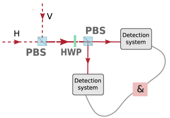
Figure 1: General scheme describing the setup for characterizing the output of the polarization HOM interferometer: Distinguishable polarization modes are combined in a common path by means of a first PBS. A half wave plate erasures the information in the polarization degree of freedom and a second PBS projects the two polarization modes for detection

The polarization HOM interferometer is an alternative version in which polarization modes $H$ (horizontal) and $V$ (vertical) play the same role as path modes in the traditional HOM interferometer.

Photons with orthogonal polarization travel in orthogonal directions towards the two input faces of the PBS. Due to the nature of the PBS, the horizontally polarized photons will be transmitted, and the vertically polarized ones will be reflected. This means that the two beams are combined into the same output path. Immediately after the PBS, a half-wave plate is placed on the photons path allowing the rotation of the polarization state of the entering photons, adding an arbitrary phase difference between the two polarization modes. Finally, a second PBS is placed after the HWP. Photons are detected at each output of the PBS with individual photon detectors.

Therefore, the first PBS allows for the combination of both beams into a single path. In this way, interference occurs in the polarization degree of freedom while the path modes are assumed indistinguishable, in principle. Polarization interference occurs with the combination of the HWP followed by the second PBS. Under the assumption that the PBS is balanced, the transformation of the creation operators $\hat{a}^{\dagger}$ in each mode is uniquely defined by the angle of the HWP:

$$\begin{pmatrix}\hat{a}^{\dagger}_{s_{3}}\\ \hat{a}^{\dagger}_{s_{4}}\end{pmatrix}=-i\begin{pmatrix}\cos(2\theta)&\sin(2\theta)\\ \sin(2\theta)&-\cos(2\theta)\end{pmatrix}\begin{pmatrix}\hat{a}^{\dagger}_{s_{1}}\\ \hat{a}^{\dagger}_{s_{2}},\end{pmatrix},$$ (12)

where modes $s_{1},s_{2},s_{3},s_{4}$ describe linear polarization states and where $\theta=\phi/4$ is the physical angle of the HWP. For the particular case of $\theta=\pi/8$ ($\phi=\pi/2$), the matrix in (12) is equivalent to that of a balanced beam splitter. Then, by adjusting the angle of the half-wave plate, it is possible to introduce a relative phase difference between the polarization modes of the photons in the input state, generating an interference pattern.

We will assume that photons are generated in pairs. In the simplest case, the four photons arrive at the HWP at the same time, two photons with polarization $s_{1}$ and other two photons with polarization $s_{2}$. In a case closer to the experimental conditions, the photons can differ in their spatiotemporal modes and their frequency; then the photon wave packet operator formalism is used to find the probability distribution of each state. After interacting with the first PBS, the four photons are combined in a single path mode and the initial state

$$\ket{\psi^{\mathrm{in}}}=\ket{2_{\xi_{1}}}_{s_{1}}\ket{2_{\xi_{2}}}_{s_{2}}$$ (13)

is generated, where two photons are in mode $\xi_{1}$ with polarization $s_{1}$ and the other two photons are in mode $\xi_{2}$ with polarization $s_{2}$.

The probability distributions are then described by the aforementioned correlation functions, with the corresponding observables. The general expression for the fourth order correlation function is given by:

$$G^{(4)}(t_{1},t_{2},t_{3},t_{4})=\sum_{s,s^{\prime},s^{\prime\prime},s^{\prime\prime\prime}}tr\left[\hat{A}_{s,s^{\prime},s^{\prime\prime},s^{\prime\prime\prime}}(t_{1},t_{2},t_{3},t_{4})\rho^{\mathrm{in}}\right],$$ (14)

where $\hat{A}(t_{1},t_{2},t_{3},t_{4})$ is the temporal correlation operator that describes the arrival of photons with polarization along arbitrary directions $s,s^{\prime},s^{\prime\prime},s^{\prime\prime\prime}$ to the detectors at each time $t_{1},t_{2},t_{3},t_{4}$ respectively, and can be expressed in terms of the photon wave packet operators:

$$\hat{A}_{s,s^{\prime},s^{\prime\prime},s^{\prime\prime\prime}}(t_{1},t_{2},t_{3},t_{4})=\hat{a}_{s}^{\dagger}(t_{1})\hat{a}_{s^{\prime}}^{\dagger}(t_{2})\hat{a}_{s^{\prime\prime}}^{\dagger}(t_{3})\hat{a}_{s^{\prime\prime\prime}}^{\dagger}(t_{4})\hat{a}_{s^{\prime\prime\prime}}(t_{4})\hat{a}_{s^{\prime\prime}}(t_{3})\hat{a}_{s^{\prime}}(t_{2})\hat{a}_{s}(t_{1}).$$ (15)

This operator is different for each detection configuration at the output of the second PBS, where photons can be distributed in each of the two output faces of the PBS according to their polarization. We can differentiate 3 cases, with the following corresponding operators:

• $\hat{A}^{4:0}_{s_{3},s_{3},s_{3},s_{3}}$ where all four photons are polarized in the direction $s_{3}$. This term will contribute to the probability of detecting state $\ket{4}_{s_{3}}\ket{0}_{s4}\equiv\ket{4,0}$. The case of state $\ket{0,4}$ is equivalent.

• $\hat{A}^{3:1}_{s_{3},s_{3},s_{3},s_{4}}$ where three photons exit the PBS through the same path mode with their polarization oriented along direction $s_{3}$, while one photon exits the PBS through the other path mode with polarization direction $s_{4}$, orthogonal to $s_{3}$. This operator describes the probability distribution associated to state $\ket{3,1}$ (case $\ket{1,3}$ is equivalent).

• $\hat{A}^{2:2}_{s_{3},s_{3},s_{4},s_{4}}$ where two photons are polarized along direction $s_{3}$ at the output of the PBS, while the other two photons are oriented along the orthogonal polarization direction $s_{4}$ at the other output path of the PBS. This observable describes the probability of detecting the state $\ket{2,2}$.

All these operators can be expressed in terms of the input operators using (12). In this way, each probability distribution can be calculated, obtaining (see Appendix A for a detailed calculation):

$$\begin{aligned} \hfil\displaystyle\begin{split}P^{(4,4:0)}&(\theta,\delta\tau,\delta\omega)=\cos^{4}(2\theta)\sin^{4}(2\theta)\left(1+e^{-\frac{8\delta\tau^{2}}{t_{c}^{2}}-2\,\delta\omega^{2}t_{c}^{2}}+4e^{-\frac{4\delta\tau^{2}}{t_{c}^{2}}-\delta\omega^{2}t_{c}^{2}}\right),\end{split}\end{aligned}$$ (16a)

$$\begin{aligned} \hfil\displaystyle\begin{split}P^{(4,3:1)}&(\theta,\delta\tau,\delta\omega)=2\cos^{2}(2\theta)\sin^{2}(2\theta)\Bigg{(}\sin^{4}(2\theta)+\cos^{4}(2\theta)+\\ &+2(\sin^{2}(2\theta)-\cos^{2}(2\theta))^{2}e^{-\frac{4\delta\tau^{2}}{t_{c}^{2}}-\delta\omega^{2}t_{c}^{2}}-2\cos^{2}(2\theta)\sin^{2}(2\theta)e^{-\frac{8\delta\tau^{2}}{t_{c}^{2}}-2\,\delta\omega^{2}t_{c}^{2}}\Bigg{)},\end{split}\end{aligned}$$ (16b)

$$\begin{aligned} \hfil\displaystyle\begin{split}P^{(4,2:2)}&(\theta,\delta\tau,\delta\omega)=\sin^{8}(2\theta)+4\cos^{4}(2\theta)\sin^{4}(2\theta)+\cos^{8}(2\theta)+\\ &+8\left(\sin^{4}(2\theta)\cos^{4}(2\theta)-\cos^{6}(2\theta)\sin^{2}(2\theta)-\sin^{6}(2\theta)\cos^{2}(2\theta)\right)e^{-\frac{4\delta\tau^{2}}{t_{c}^{2}}-\delta\omega^{2}t_{c}^{2}}+\\ &+6\sin^{4}(2\theta)\cos^{4}(2\theta)e^{-\frac{8\delta\tau^{2}}{t_{c}^{2}}-2\,\delta\omega^{2}t_{c}^{2}},\end{split}\end{aligned}$$ (16c)

with $\delta\omega=(\omega_{2}-\omega_{1})/2$ and $\delta\tau=(\tau_{2}-\tau_{1})/2$, being $\tau_{1,2}$ the times at which each photon pair arrives at the HWP. To better understand these distributions, Fig. 2 shows each one as a function of the phase difference given by the angle of the HWP $\theta$ and the path length difference, where we used $\delta\tau=\delta z/c$. In all cases we assumed $\delta\omega=0$, that is, frequency indistinguishability, and $t_{c}=l_{c}/c$ with $l_{c}=60\mu m$ the coherence length of the photon wave packet.

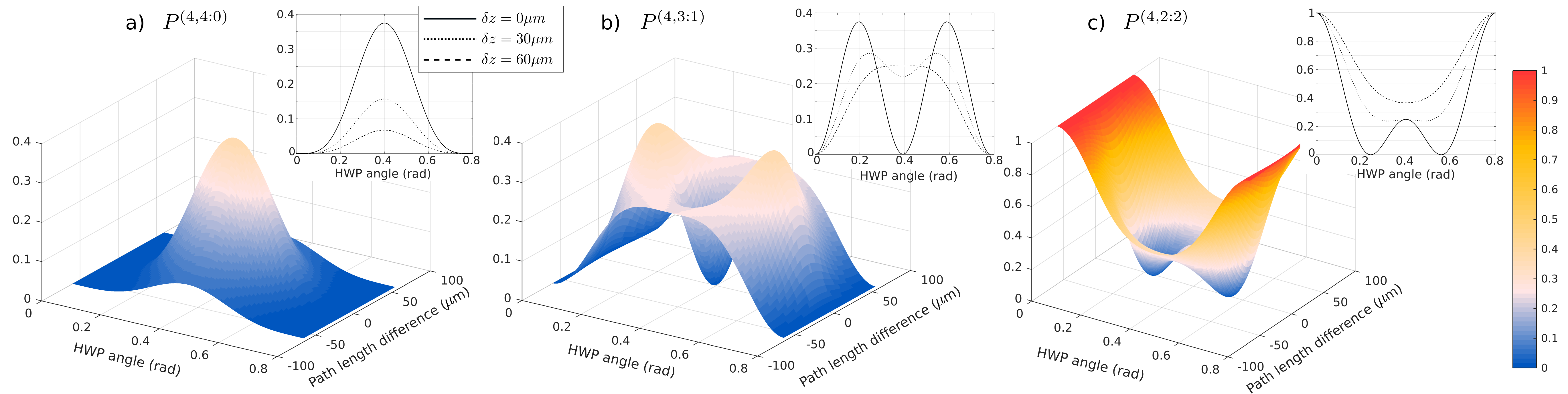
Figure 2: Probability distributions a) $P^{(4,4:0)}$; b) $P^{(4,3:1)}$ and c) $P^{(4,2:2)}$ as a function of the phase difference given by the angle of the HWP $\theta$ on the $x$ axis and the path length difference $\delta z$ on the $y$ axis. The insets correspond to cuts in the $y$ axis for three particular cases of $\delta z=0\mu m$ (solid line); $\delta z=30\mu m$ (dotted line) and $\delta z=60\mu m$ (dashed line).

From these figures, it can be observed that the probability distributions exhibit a high sensitivity to variations in the parameter $\theta$. In particular, for indistinguishable photon paths ($\delta z=0$), $P^{(4,4:0)}$ achieves its maximum value for $\theta=\pi/8$, while $P^{(4,3:1)}$ reaches a minimum zero value, contributing to the four-photon bunching interference. In analogy to the two photon HOM effect, we would also expect $P^{(4,2:2)}$ to have a minimum at this point. On the contrary, $P^{(4,2:2)}$ shows an enhancement at $\theta=\pi/8$ and two (minimum) zero values located symmetrically with respect to this point. This effect has already been reported [10, 11], proving that when four particles interfere simultaneously there is a non-monotonic transition as the photons become distinguishable. In our case, this behaviour arises as the polarization modes become orthogonal, even though the photon paths are indistinguishable. The non-monotonic behaviour can also be seen for $P^{(4,3:1)}$ as a function of the phase difference. An interesting effect that can be observed is that the interference patterns behave differently if the distinguishing information arises in the polarization or in the path degree of freedom. For completely distinguishable photon paths, we can still observe a phase modulation, while for orthogonal polarization modes interference vanishes completely in the path degree of freedom. Also, for complete indistinguishability in the photon’s path, the non-monotonic behaviour is present in both $P^{(4,3:1)}$ and $P^{(4,2:2)}$, while for indistinguishable polarization modes this non-monotonic transition is only seen for $P^{(4,2:2)}$.

As the path length difference increases, the pattern close to $\theta=\pi/8$ experiences fewer fluctuations and becomes more uniform, implying that the system loses the ability to record changes in $\theta$. To describe how these probability distributions (16) affect the precision achievable in the problem of phase estimation, and to quantify the sensitivity of interference mentioned above, we will use the Fisher information.

II.3 Phase estimation and quantum Fisher information

The Fisher information (FI) quantifies the information encoded in an estimation process based on the probability distribution. The lower bound for the variance of the estimated parameter $\hat{\phi}$ is given by the quantum Cramér-Rao bound [25, 26] (QCRB):

$$\Delta^{2}(\hat{\phi})\geq\frac{1}{F_{Q}(\phi)},$$ (17)

where $F_{Q}(\phi)=\max_{\{\mathcal{M}\}}F(\phi)$ is the quantum Fisher information (QFI), and $F(\phi)$ the Fisher information defined as:

$$F(\phi)=\sum_{m}\frac{1}{p(m|\phi)}\left|\frac{dp(m|\phi)}{d\phi}\right|^{2}.$$ (18)

The QFI is then determined from the corresponding probabilities $p(m|\phi)=\mathrm{tr}[M_{m}\hat{\rho}_{\phi}]$ associated to a positive-operator valued measure (POVM) $\mathcal{M}=\{M_{m}\}$ (with possible outcomes $m$) for the given state $\hat{\rho}_{\phi}$, and the maximum is taken over all possible POVMs ${\{\mathcal{M}\}}$. Therefore, the QFI quantifies the maximal information on the parameter to be estimated.

For the particular case of phase estimation $\phi$ from the unitary evolution $U_{\phi}=\exp(-i\phi H)$, and for an arbitrary initial pure state $\rho^{\mathrm{in}}=\ket{\Phi^{\mathrm{in}}}\bra{\Phi^{\mathrm{in}}}$, the QFI is proportional to the variance of the Hamiltonian in the initial state and does not depend on $\phi$. That is, $F_{Q}(\ket{\Phi^{\mathrm{in}}})=4\Delta^{2}(H)$ with $\Delta^{2}(H)=\braket{\Phi^{\mathrm{in}}|H^{2}|\Phi^{\mathrm{in}}}-\left(\braket{\Phi^{\mathrm{in}}|H|\Phi^{\mathrm{in}}}\right)^{2}$ [27, 16].

In this paper, we focus on the problem of phase estimation inside a two-port interferometer using an input state with a definite number of photons ($N$). It has been shown [28] that for the input state given by Ec. (11), that is, $\ket{\Phi^{\mathrm{in}}}=\ket{\psi_{HB}}$ the QFI is given by

$$F_{Q}(\ket{\psi_{HB}},N)=N(N/2+1),$$ (19)

such that the variance scales as the Heisenberg limit ($\Delta^{2}(\hat{\phi})\sim 1/N^{2}$).

To evaluate the phase sensitivity in our scheme, we used the Fisher information defined as:

$$F(\phi)=\sum_{m}\frac{1}{P^{(4,m)}(\phi)}\left(\frac{\partial P^{(4,m)}(\phi)}{\partial\phi}\right)^{2}$$ (20)

with $m\in\left\{4:0,0:4,3:1,1:3,2:2\right\}$ and the probabilities given by Ec. (16), with $\theta=\phi/4$.

The Fisher information (20) can be calculated as a function of the phase difference $\phi\in[0,\pi]$ for different values of the path length difference $\delta z\in[0,l_{c}]$ (see Fig. 3). For complete indistinguishability ($\delta z=0$) we obtain $F(\phi)\equiv 12\quad\forall\quad\phi$, which is exactly the value of the QFI in Ec. (19) for $N=4$: $F_{Q}(\phi)=12$. Therefore, for indistinguishable photons, the maximum precision is achieved for the selected POVM and it is independent of the parameter to be estimated.

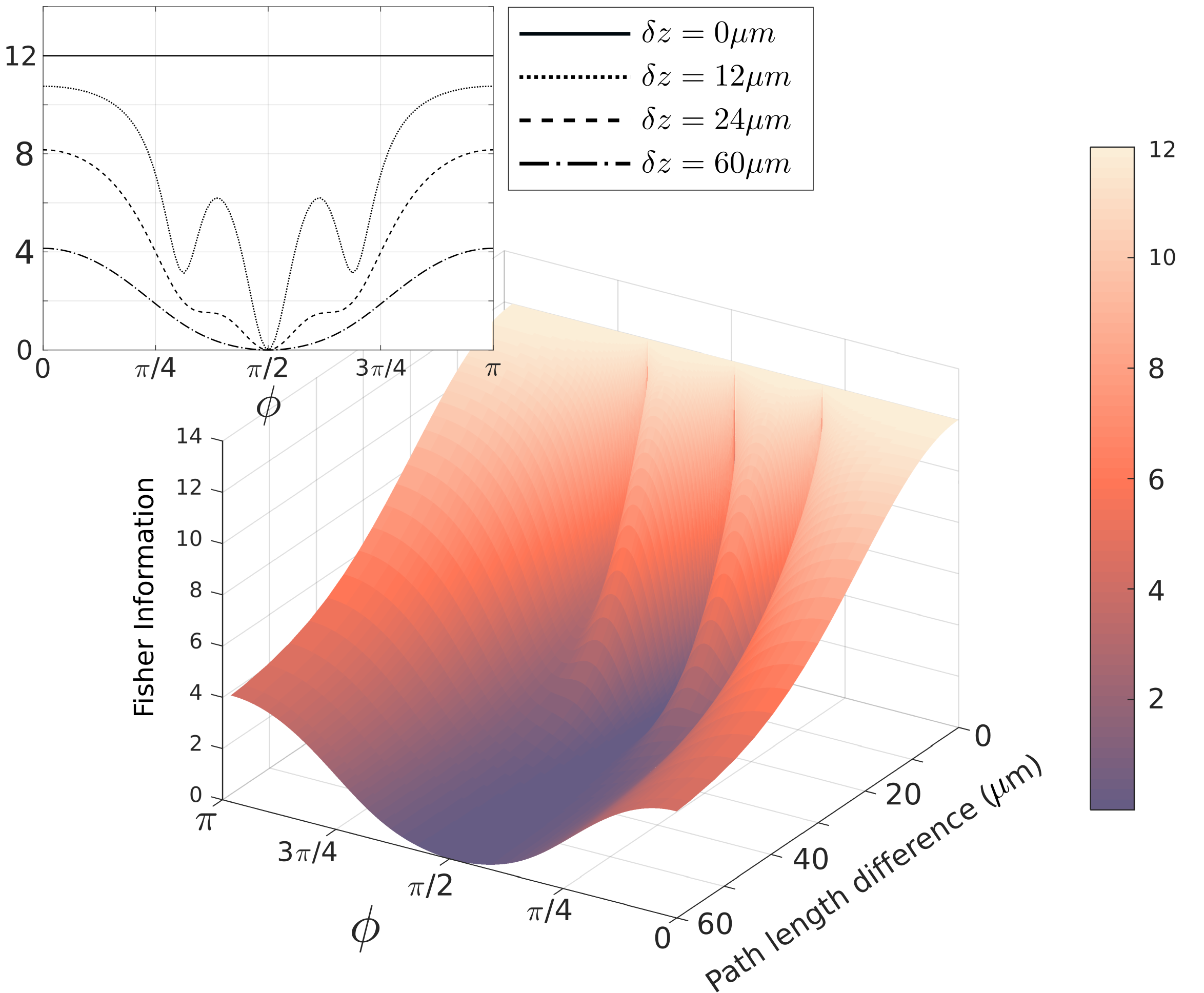
Figure 3: Fisher information as a function of the phase difference $\phi$ and the path length difference $\delta z$. For indistinguishable photons ($\delta z$=0) a maximum value of $F=12$ is achieved for all phase values. With increasing indistinguishability (as the path length difference increases) the FI decreases and becomes dependent on the phase. This can be seen on the inset for four different values of $\delta z$.

As the path length difference increases, the Fisher information decreases and a dependence with the phase also appears. When $\delta z\geq l_{c}$ the Fisher information reaches the SQL ($F(\phi)=4$) for certain phase values, as can be seen on the inset of Fig. 3. For all values of $\delta z\neq 0$ the Fisher information goes to zero for $\phi=\pi/2$. As mentioned before, as the path difference increases and the phase difference is close to $\phi=\pi/2$ ($\theta=\pi/8$) the system becomes less sensitive to changes in the phase, losing precision in its estimation.

An interesting feature that can be seen from these figures is that for indistinguishable photon paths ($\delta z=0$), the probability distributions present a high sensitivity to variations in the phase, while the FI remains constant and equal to the ultimate value given by the QFI for our particular scheme, even in the presence of a non-monotonic behaviour in the phase as the ones given by $P^{(4,2:2)}$ and $P^{(4,3:1)}$. This suggests that the enhancement on the precision is achieved by interference patterns exhibiting significant variations in the phase.

For the particular case of $N/2$ photons per input mode in a two-port interferometer it has been shown that the QFI increases linearly with respect to the degree of indistinguishability $\mathcal{I}$, and does not depend on the phase $\phi$ to be estimated: $F_{Q}(\phi)=N\left(\frac{N}{2}\mathcal{I}+1\right)$ [29, 30]. This result shows that, for a given POVM, the FI can be found to be independent of the phase for all values of $\mathcal{I}$ (given by the path length difference). The chosen POVM in our scheme does not attain the QFI, except for $\delta z=0$ ($\mathcal{I}=1$). Nonetheless, for certain phase values, the multi-photon state enables higher values of FI compared to the QFI in the best two-particles scenario, achieving higher precisions in the estimation process.

III Experiment and Results

As described in the previous Section II.2, our experimental scheme (Fig. 4a)) consists of three parts: i) a photon pair source; ii) a polarization based interferometer; iii) a detection system. Photon pairs are generated by Spontaneous Parametric Down Conversion (SPDC) in a BBO type-I nonlinear crystal pumped by a CW 405 nm vertically polarized laser (120 mW). Pairs of horizontally polarized photons are generated at 810 nm and directed into two distinct path modes.

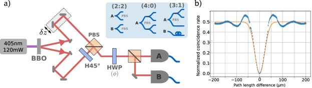
Figure 4: a) Experimental setup consisting of a photon pair source generating horizontally polarized photons by SPDC. These photons are then recombiend into a single path mode by means of a HWP at 45^∘ and a PBS. Polarization interference is then achieved by a HWP adding a phase difference $\phi$ between both polarization modes. Photons are then projected by a PBS into the output modes and coupled to FBSs assembled in different configurations associated to each probability measurement (outlined in the blue inset). b) HOM interference: Two-fold coincidences as a function of the path length difference. The blue dots correspond to the normalized coincidence counts after background subtraction. The peaks on each side of the dip are caused by the rectangular shape of the interference filters used in the experiment. Error bars were calculated assuming the count rates follow a Poisson distribution. The solid line corresponds to the fitted two-photon coincidence probability distribution.

Our photon pair source has an effective coincidence/single count ratio of $0.30\pm 0.02$, with a maximum two-fold coincidence count rate of 150 kHz. The measured four-fold coincidence rate was 45 Hz. These coincidences were obtained using fiber beam splitters (FBS) coupled to each path, four single photon detectors (Si APD) and an FPGA-based coincidence counter. 10 nm interference filters were placed before the coupling to each FBS. The coincidence time window was 20 ns, determined by the FPGA’s internal clock.

The generated photons in each of the two paths are then recombined into a single path mode by use of a HWP at $45^{\circ}$ in one of the paths, that rotates the horizontally polarized photons into vertically polarized ones, followed by a PBS. In this way, the vertically polarized photons are reflected by the PBS and the horizontally polarized photons on the other path are transmitted into the same output path after the PBS (see Fig. 4a)).

The polarization-based interferometer is implemented as described in Section II.2. The output state is detected with four Si APDs. Each probability distribution in Eq. (16) is detected individually using FBSs in a tree configuration in order to resolve each contribution (see inset in Fig. 4a)).

By measuring the two-fold coincidences as a function of the path length difference for $\phi=\pi/2$ ($\theta=\pi/8$), the traditional two-photon HOM interference effect can be observed and used to define indistinguishability. Fig. 4b) shows the normalized coincidence counts as a function of the path length difference (blue dots). The solid line corresponds to the fitted two-photon coincidence probability distribution [22]. The obtained visibility is $0.998\pm 0.001$. The observed oscillations outside the dip correspond to the spectral filtering given by the use of rectangular-shaped interference filters and the fiber coupling.

Measurements of the probability distributions $P^{(4,2:2)}$, $P^{(4,3:1)}$ and $P^{(4,4:0)}$ as a function of the HWP angle (phase difference) were taken for both a) indistinguishable ($\delta z=0$) and b) distinguishable ($\delta z>60\mu m$) cases, shown in Figure 5. Symbols represent the measured probabilities, calculated from the normalized count rates, while the dashed lines correspond to the fitted probabilities according to (16).

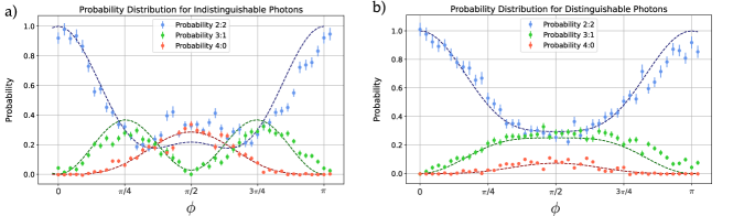
Figure 5: Probability distributions $P^{(4,2:2)}$ (blue), $P^{(4,3:1)}$ (green) and $P^{(4,4:0)}$ (red) for a) indistinguishable and b) distinguishable photons as a function of the phase difference $\phi$. Symbols represent the calculated probabilities from the measured count rates while the dashed lines correspond to the fitted probabilities according to (16).

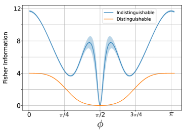
Figure 6: Fisher information for four indistinguishable (blue) and distinguishable (orange) photons as a function of the parameter $\phi$. Shaded area corresponds to the uncertainty estimated by Monte Carlo simulations (for the distinguishable case errors are smaller than the line width).

From the fitted probability distributions the parameters $\delta\lambda$ and $\delta z$ for the case of maximum indistinguishability were determined to be 10 nm and 10 $\mu$m, respectively. The value for $\delta\lambda$ is within the FWHM of the interference filters used in the detection system, while the value of $\delta z$ differs from the desired optimal conditions due to noise and other experimental imperfections, especially for the case of $P^{(4,2:2)}$, which shows considerable background noise affecting the visibility and sensitivity of the measurements.

The Fisher information was then calculated from the fitted probability distributions as a function of the phase difference $\phi$ using (20), for both indistinguishable and distinguishable photons. The obtained values are shown in Fig. 6. The shaded area corresponds to the uncertainty in the FI, calculated by Monte Carlo simulations of experimental runs with the same statistics as the measured count rates.

For both cases the FI exhibits fluctuations with respect to the parameter $\phi$. This behaviour is expected given that complete indistinguishability was not achieved, as mentioned above, making the FI no longer independent of the parameter to be estimated (see Fig. 3). The maximum value is achieved for $\phi=0,\pi$ in both cases, obtaining $F^{4,ind}=11.6\pm 0.1$ and $F^{4,dis}=3.998\pm 0.002$. Despite fluctuations, the FI for indistinguishable photons surpasses de one for distinguishable photons for every phase value other than $\phi=\pi/2$.

IV Concluding remarks

We presented theoretical and experimental results for the problem of parameter estimation using a four-photon Holland-Burnett probe state. We have described the correlation functions needed to calculate the probability distributions associated with our experimental scheme. These were calculated as a function of different degrees of freedom, which contribute to the indistinguishability of the photons. Our characterization allows a complete description of the attainable precision in the problem of parameter estimation using this multi-photon state as the input probe in a HOM experiment.

For the case of completely indistinguishable photons, the probability distributions show significant variations in the phase, presenting non-monotonic behaviors. Our measurement scheme achieves the maximum precision, given by the QFI, for all phase values: $F(\phi)=F_{Q}(\phi)=12\quad\forall\quad\phi$. As the path length difference increases, the interference patterns exhibit fewer fluctuations with the phase, suggesting that the system becomes less sensitive to changes in $\phi$. As a consequence, the FI decreases and becomes dependent with the phase. These results are observed experimentally, where complete indistinguishability is hard to achieve. Nevertheless, a maximum precision given by $F^{4,ind}=11.6\pm 0.1$ was calculated for the experimentally generated indistinguishable four-photon state, surpassing the SQL estimated from the distinguishable photon case were we obtained $F^{4,dis}=3.998\pm 0.002$.

Our results contribute to the understanding of multi-particle interference and its impact in the problem of parameter estimation. The general framework presented in this work is of great relevance to photonic quantum metrology where photon interference is a crucial resource to access higher precisions than those determined by classical states.

Appendix A Probability distributions

In order to calculate each of the probabilities in equation (16) for different outputs of a two-photon pairs per input polarizing beamsplitter one have to obtain the specific fourth order correlation function, which is determined by the input state and detection configuration, which defines a specific temporal correlation operator $\hat{A}$. We subsequently show how to obtain the probability of detecting four photons with the same polarization $P^{(4,4:0)}$. The corresponding four-photon temporal correlation operator, assuming $s_{3}$ output polarization is therefore:

$$\hat{A}_{s3,s3,s3,s3}^{(4)}(t_{1},t_{2},t_{3},t_{4})=\frac{1}{\sqrt{4!}}\hat{a}_{s3}^{\dagger}(t_{1})\hat{a}_{s3}^{\dagger}(t_{2})\hat{a}_{s3}^{\dagger}(t_{3})\hat{a}_{s3}^{\dagger}(t_{4})\frac{1}{\sqrt{4!}}\hat{a}_{s3}(t_{4})\hat{a}_{s3}(t_{3})\hat{a}_{s3}(t_{2})\hat{a}_{s3}(t_{1})$$ (21)

According to (12), the operator for the $s_{3}$ output mode can be expressed in terms of the input modes as

$$\hat{a}_{3}^{\dagger}(t_{i})=-i\left[\cos(2\theta)\hat{a}_{1}^{\dagger}(t_{i})+\sin(2\theta)\hat{a}_{2}^{\dagger}(t_{i})\right],$$ (22)

where the “$s$” label has been omitted for simplicity of notation. Consequently we can express $\hat{A}$ in terms of the input operators:

$$\begin{split}\hat{A}_{3,3,3,3}^{(4)}(t_{1},t_{2},t_{3},t_{4})=&\frac{1}{4!}\left[\cos(2\theta)\hat{a}_{1}^{\dagger}(t_{1})+\sin(2\theta)\hat{a}_{2}^{\dagger}(t_{1})\right]\times\left[\cos(2\theta)\hat{a}_{1}^{\dagger}(t_{2})+\sin(2\theta)\hat{a}_{2}^{\dagger}(t_{2})\right]\\ &\times\left[\cos(2\theta)\hat{a}_{1}^{\dagger}(t_{3})+\sin(2\theta)\hat{a}_{2}^{\dagger}(t_{3})\right]\times\left[\cos(2\theta)\hat{a}_{1}^{\dagger}(t_{4})+\sin(2\theta)\hat{a}_{2}^{\dagger}(t_{4})\right]\\ &\times\Big{[}\cos(2\theta)\hat{a}_{1}(t_{4})+\sin(2\theta)\hat{a}_{2}(t_{4})\Big{]}\times\Big{[}\cos(2\theta)\hat{a}_{1}(t_{3})+\sin(2\theta)\hat{a}_{2}(t_{3})\Big{]}\\ &\times\Big{[}\cos(2\theta)\hat{a}_{1}(t_{2})+\sin(2\theta)\hat{a}_{2}(t_{2})\Big{]}\times\Big{[}\cos(2\theta)\hat{a}_{1}(t_{1})+\sin(2\theta)\hat{a}_{2}(t_{1})\Big{]}.\end{split}$$ (23)

Upon distribution of all the products of sums, it must be noticed that, since the input state is a two-photon state on each mode,

$$\ket{\psi^{\mathrm{in}}}=\ket{2_{\xi_{1}}}_{1}\ket{2_{\xi_{2}}}_{2}\propto\left(\hat{a}^{\dagger}_{\xi_{1}}\right)^{2}\left(\hat{a}^{\dagger}_{\xi_{2}}\right)^{2}\ket{0},$$ (24)

several terms of (23) will vanish; namely all the terms involving three or more creation or destruction operators. For this particular selection of input and output states the temporal correlation operator takes the form

$$\begin{split}\hat{A}_{3,3,3,3}^{(4)}(t_{1},t_{2},t_{3},t_{4})=\frac{\cos^{4}(2\theta)\sin^{4}(2\theta)}{24}&\Big{[}\hat{a}_{1}^{\dagger}(t_{1})\hat{a}_{1}^{\dagger}(t_{2})\hat{a}_{2}^{\dagger}(t_{3})\hat{a}_{2}^{\dagger}(t_{4})+\hat{a}_{2}^{\dagger}(t_{1})\hat{a}_{2}^{\dagger}(t_{2})\hat{a}_{1}^{\dagger}(t_{3})\hat{a}_{1}^{\dagger}(t_{4})\\ &+\hat{a}_{2}^{\dagger}(t_{1})\hat{a}_{1}^{\dagger}(t_{2})\hat{a}_{1}^{\dagger}(t_{3})\hat{a}_{2}^{\dagger}(t_{4})+\hat{a}_{2}^{\dagger}(t_{1})\hat{a}_{1}^{\dagger}(t_{2})\hat{a}_{2}^{\dagger}(t_{3})\hat{a}_{1}^{\dagger}(t_{4})\\ &+\hat{a}_{1}^{\dagger}(t_{1})\hat{a}_{2}^{\dagger}(t_{2})\hat{a}_{1}^{\dagger}(t_{3})\hat{a}_{2}^{\dagger}(t_{4})+\hat{a}_{1}^{\dagger}(t_{1})\hat{a}_{2}^{\dagger}(t_{2})\hat{a}_{2}^{\dagger}(t_{3})\hat{a}_{1}^{\dagger}(t_{4})\Big{]}\\ &\times\Big{[}\hat{a}_{1}(t_{4})\hat{a}_{1}(t_{3})\hat{a}_{2}(t_{2})\hat{a}_{2}(t_{1})+\hat{a}_{1}(t_{4})\hat{a}_{2}(t_{3})\hat{a}_{1}(t_{2})\hat{a}_{2}(t_{1})\\ &+\hat{a}_{1}(t_{4})\hat{a}_{2}(t_{3})\hat{a}_{2}(t_{2})\hat{a}_{1}(t_{1})+\hat{a}_{2}(t_{4})\hat{a}_{1}(t_{3})\hat{a}_{1}(t_{2})\hat{a}_{2}(t_{1})\\ &+\hat{a}_{2}(t_{4})\hat{a}_{1}(t_{3})\hat{a}_{2}(t_{2})\hat{a}_{1}(t_{1})+\hat{a}_{2}(t_{4})\hat{a}_{2}(t_{3})\hat{a}_{1}(t_{2})\hat{a}_{1}(t_{1})\Big{]}.\end{split}$$ (25)

The corresponding fourth order correlation function can be calculated as

$$G^{(4)}(t_{1},t_{2},t_{3},t_{4})=\bra{\psi^{\mathrm{in}}}\hat{A}_{3,3,3,3}^{(4)}(t_{1},t_{2},t_{3},t_{4})\ket{\psi^{\mathrm{in}}};$$ (26)

when the product of sums in (25) is distributed, a sum of 36 terms is obtained. Each of these terms $g$ has the form of

$$g=\frac{\cos^{4}(2\theta)\sin^{4}(2\theta)}{24}\cdot\bra{2_{\xi_{1}}}_{1}\bra{2_{\xi_{2}}}_{2}\hat{a}_{i}^{\dagger}(t_{1})\hat{a}_{j}^{\dagger}(t_{2})\hat{a}_{k}^{\dagger}(t_{3})\hat{a}_{l}^{\dagger}(t_{4})\hat{a}_{i^{\prime}}(t_{4})\hat{a}_{j^{\prime}}(t_{3})\hat{a}_{k^{\prime}}(t_{2})\hat{a}_{l^{\prime}}(t_{1})\ket{2_{\xi_{1}}}_{1}\ket{2_{\xi_{2}}}_{2}$$ (27)

where $\{i,j,k,l\}$ and $\{i^{\prime},j^{\prime},k^{\prime},l^{\prime}\}$ run over the six permutations of the sequence $\{1,1,2,2\}$. Using standard properties of number states and creation and destruction operators and re-ordering the product of scalar terms, each term $g$ of the sum can be written in terms of the temporal wavepackets of each input mode, and we obtain an expression that is separable in the variables $t_{1}$, $t_{2}$, $t_{3}$ and $t_{4}$.

$$g=\frac{4\cos^{4}(2\theta)\sin^{4}(2\theta)}{24}\xi_{i}^{*}(t_{1})\xi_{l^{\prime}}(t_{1})\cdot\xi_{j}^{*}(t_{2})\xi_{k^{\prime}}(t_{2})\cdot\xi_{k}^{*}(t_{3})\xi_{j^{\prime}}(t_{3})\cdot\xi_{l}^{*}(t_{4})\xi_{i^{\prime}}(t_{4}).$$ (28)

The four-photon detection probability $P^{(4,4:0)}$ can be calculated, in the limit of the detection time $\Delta t_{0}$ much larger than the coherence time of the wavepacket $t_{c}$, by integrating the fourth order correlation function $G^{(4)}$:

$$P^{(4)}=\iiiint dt_{1}dt_{2}dt_{3}dt_{4}\,G^{(4)}(t_{1},t_{2},t_{3},t_{4}).$$ (29)

It should be noted that permutation of the mode indexes in (28) leads to different expressions depending on whether the modes on the products $\xi_{i}^{*}(t)\xi_{j}(t)$ are similar or not. The expression for $P^{(4)}$ can then be rearranged as

$$\begin{split}P^{(4,4:0)}=&\frac{\cos^{4}(2\theta)\sin^{4}(2\theta)}{6}\left\{6\,\left(\int\left|\xi_{1}(t)\right|^{2}dt\right)^{2}\cdot\left(\int\left|\xi_{2}(t)\right|^{2}dt\right)^{2}\right.\\ &+6\,\Re\left(\int\left|\xi_{1}(t)\right|^{2}dt\cdot\int\left|\xi_{2}(t)\right|^{2}dt\cdot\int\xi^{*}_{1}(t)\xi_{2}(t)dt\cdot\int\xi^{*}_{2}(t)\xi_{1}(t)dt\right)\\ &\left.+24\,\Re\left[\left(\int\xi^{*}_{1}(t)\xi_{2}(t)dt\right)^{2}\cdot\left(\int\xi^{*}_{2}(t)\xi_{1}(t)dt\right)^{2}\right]\right\}.\end{split}$$ (30)

This expression allows for the calculation of the probability of obtaining a four-photon output at one of the outputs as a function of several parameters of the photon wavepackets, such as the temporal width, the central frequency and the arrival time of the input states. We assume Gaussian temporal wavepackets for both input modes of the form

$$\xi_{k}(t)=\left(\frac{2}{\pi t_{c}^{2}}\right)^{1/4}\exp{\left[-\frac{\left(t-\delta\tau_{k}\right)^{2}}{t_{c}^{2}}-i\omega_{k}\left(t-\delta\tau_{k}\right)\right]}$$ (31)

where $t_{c}$ is the coherence time of the wavepackets, which is inversely proportional to their bandwith, $\delta\tau_{1}=-\delta\tau_{2}\equiv\delta\tau$ are the arrival times of (the two) input modes, $\omega_{k}$ is the central optical frequency of each mode and the frequency difference is $\delta\omega=(\omega_{2}-\omega_{1})/2$. The probability of obtaining four photons at a single output is therefore

$$P^{(4,4:0)}(2\theta,t_{c},\delta\tau,\delta\omega)=\cos^{4}(2\theta)\sin^{4}(2\theta)\left(1+e^{-\frac{8\delta\tau^{2}}{t_{c}^{2}}-2\,\delta\omega^{2}t_{c}^{2}}+4e^{-\frac{4\delta\tau^{2}}{t_{c}^{2}}-\delta\omega^{2}t_{c}^{2}}\right).$$ (32)

In order to calculate the probabilities of the other detection configurations at the output, namely $P^{(4,3:1)}$ and $P^{(4,2:2)}$, the correlation operator has to be modified accordingly:

$$\hat{A}_{3,3,3,4}^{(4)}(t_{1},t_{2},t_{3},t_{4})=\frac{1}{\sqrt{3!}}\hat{a}_{3}^{\dagger}(t_{1})\hat{a}_{3}^{\dagger}(t_{2})\hat{a}_{3}^{\dagger}(t_{3})\hat{a}_{4}^{\dagger}(t_{4})\frac{1}{\sqrt{3!}}\hat{a}_{4}(t_{4})\hat{a}_{3}(t_{3})\hat{a}_{3}(t_{2})\hat{a}_{3}(t_{1})$$ (33)

and

$$\hat{A}_{3,3,4,4}^{(4)}(t_{1},t_{2},t_{3},t_{4})=\frac{1}{\sqrt{2!}\sqrt{2!}}\hat{a}_{3}^{\dagger}(t_{1})\hat{a}_{3}^{\dagger}(t_{2})\hat{a}_{4}^{\dagger}(t_{3})\hat{a}_{4}^{\dagger}(t_{4})\frac{1}{\sqrt{2!}\sqrt{2!}}\hat{a}_{4}(t_{4})\hat{a}_{4}(t_{3})\hat{a}_{3}(t_{2})\hat{a}_{3}(t_{1})$$ (34)

respectively; the operator for the $s_{4}$ output mode is

$$\hat{a}_{4}^{\dagger}(t_{i})=-i\left[\sin(2\theta)\hat{a}_{1}^{\dagger}(t_{i})-\cos(2\theta)\hat{a}_{2}^{\dagger}(t_{i})\right].$$ (35)

References

- [1] H. S. Zhong, et. al, Quantum computational advantage using photons, Science, 370, 1460-1463 (2020).
- [2] E. Polino, M. Valeri, N. Spagnolo, and F. Sciarrino, Photonic quantum metrology, AVS Quant. Sci., 2, 2 (2020).
- [3] J. L. O’brien, A. Furusawa, and J. Vučković, Photonic quantum technologies, Nat. Phot., 3, 687-695 (2009).
- [4] X. Ding, et. al, On-demand single photons with high extraction efficiency and near-unity indistinguishability from a resonantly driven quantum dot in a micropillar, Phys. Rev. Lett., 116, 020401 (2016).
- [5] N. Tomm, et. al, A bright and fast source of coherent single photons, Nat. Nanotech., 16, 399-403 (2021).
- [6] R. P. Feynman, R. B. Leighton, and M. Sands, The Feynman Lectures on Physics Vol. III, Addison Wesley (1965).
- [7] M. O. Scully, B. G. Englert, and H. Walther, Quantum optical tests of complementarity, Nature, 351, 111-116 (1991).
- [8] L. Mandel, Coherence and indistinguishability, Opt. Lett. 16(23), 1882-1883 (1991).
- [9] C. K. Hong, Z. Ou and L. Mandel, Measurement of subpicosecond time intervals between two photons by interference, Phys. Rev. Lett. 59, 2044 (1987).
- [10] M. C. Tichy, H. T. Lim, Y. S. Ra, F. Mintert, Y. H. Kim, and A. Buchleitner, Four-photon indistinguishability transition. Phys. Rev. A, 83, 062111 (2011).
- [11] Y.-S. Ra, M. C. Tichy, H.-T. Lim, O. Kwon, F. Mintert, A. Buchleitner and Y.-H. Kim, Nonmonotonic quantum-to-classical transition in multiparticle interference, PNAS 110, 1227 (2013).
- [12] A. E. Jones, A. J. Menssen, H. M. Chrzanowski, T. A. Wolterink, V. S. Shchesnovich, and I. A. Walmsley, Multiparticle interference of pairwise distinguishable photons, Phys. Rev. Lett., 125, 123603 (2020).
- [13] A. J. Menssen, A. E. Jones, B. J. Metcalf, M. C. Tichy, S. Barz, W. S. Kolthammer, and I. A. Walmsley, Distinguishability and many-particle interference, Phys. Rev. Lett., 118, 153603 (2017).
- [14] A. E. Jones, S. Kumar, S. D’Aurelio, M. Bayerbach, A. J. Menssen, and S. Barz, Distinguishability and mixedness in quantum interference. Phys. Rev. A, 108, 053701 (2023).
- [15] V. Giovannetti, S. Lloyd, and L. Maccone, Quantum-enhanced measurements: beating the standard quantum limit, Science, 306, 1330-1336 (2004).
- [16] G. Tóth and I. Apellaniz1, Quantum metrology from a quantum information science perspective, J. Phys. A: Math. Theor. 47, 424006 (2014).
- [17] The LIGO Scientific Collaboration. A gravitational wave observatory operating beyond the quantum shot-noise limit, Nature Phys. 7, 962–965 (2011).
- [18] J. P. Dowling, Correlated input-port, matter-wave interferometer: Quantum-noise limits to the atom-laser gyroscope, Phys. Rev. A 57, 4736 (1998).
- [19] J. Qin, Y.-H. Deng, H.-S. Zhong, et al., Unconditional and Robust Quantum Metrological Advantage beyond N00N States, Phys. Rev. Lett. 130, 070801 (2023).
- [20] Z. Ou and X. Li, Quantum SU(1,1) interferometers: Basic principles and applications. APL Photonics, 5, 080902 (2020).
- [21] P. M. Birchall, J. Sabines-Chesterking, J. L. O’Brien, H. Cable and J. C. F. Matthews, Beating the shot-noise limit with sources of partially-distinguishable photons, arXiv:1603.00686v2 (2016).
- [22] T. Legero, T. Wilk, A. Kuhn, and G. Rempe, Characterization of single photons using two-photon interference, Adv. In At., Mol., and Opt. Phys., 53, 253-289 (2006).
- [23] R. Loudon, The quantum theory of light. OUP Oxford (2000).
- [24] M. J. Holland and K. Burnett, Interferometric detection of optical phase shifts at the Heisenberg limit, Phys. Rev. Lett. 71, 1355 (1993).
- [25] C. W. Helstrom, Minimum mean-squared error of estimates in quantum statistics, Phys. Lett. A 25, 101 (1967).
- [26] A. S. Holevo, Probabilistic and Statistical Aspects of Quantum Theory, North-Holland, Amsterdam, (1982).
- [27] M. Paris, Quantum estimation for quantum technology, Int. J. Quantum Inf 7, 125 (2009).
- [28] M. Eaton, R. Nehra, A. Win, and O. Pfister, Heisenberg-limited quantum interferometry with multiphoton-subtracted twin beams, Phys. Rev. A, 103, 013726 (2021).
- [29] L. T. Knoll, G. M. Bosyk, I. L. Grande, and M. A. Larotonda, Role of indistinguishability in interferometric phase estimation, Phys. Rev. A, 100, 062125 (2019).
- [30] L. T. Knoll and G. M. Bosyk, Simultaneous quantum estimation of phase and indistinguishability in a two-photon interferometer, JOSA B, 40, C67-C72 (2023).