Offline Critic-Guided Diffusion Policy for Multi-User Delay-Constrained Scheduling

Abstract

Effective multi-user delay-constrained scheduling is crucial in various real-world applications, such as instant messaging, live streaming, and data center management. In these scenarios, schedulers must make real-time decisions to satisfy both delay and resource constraints without prior knowledge of system dynamics, which are often time-varying and challenging to estimate. Current learning-based methods typically require interactions with actual systems during the training stage, which can be difficult or impractical, as it is capable of significantly degrading system performance and incurring substantial service costs. To address these challenges, we propose a novel offline reinforcement learning-based algorithm, named Scheduling By Offline Learning with Critic Guidance and Diffusion Generation (SOCD), to learn efficient scheduling policies purely from pre-collected offline data. SOCD innovatively employs a diffusion-based policy network, complemented by a sampling-free critic network for policy guidance. By integrating the Lagrangian multiplier optimization into the offline reinforcement learning, SOCD effectively trains high-quality constraint-aware policies exclusively from available datasets, eliminating the need for online interactions with the system. Experimental results demonstrate that SOCD is resilient to various system dynamics, including partially observable and large-scale environments, and delivers superior performance compared to existing methods.

1 Introduction

The rapid expansion of real-time applications, such as instant messaging [86], live streaming [63], and datacenter management [13], has underscored the necessity for effective multi-user delay-constrained scheduling. The quality of scheduling significantly influences user satisfaction, which, in turn, impacts the economic viability of the scheduling system. For instance, [27] demonstrates that system response time is a predominant factor in user satisfaction within information systems. Moreover, an efficient scheduling policy must adhere to resource expenditure budgets. For example, power consumption is a critical concern in scheduling problems such as datacenter maintenance [25]. A resource-efficient scheduling policy will also facilitate the development of low-carbon systems, e.g., [11, 40].

These requirements compel schedulers to make instantaneous decisions that adhere to stringent delay [41] and resource [78] constraints. The delay metric depends on the comprehensive dynamics and control of the system over time, while resource constraints add further complexity to scheduling decisions. Traditional optimizaiton-based scheduling methods, such as dynamic programming, e.g., [72, 8], and Lyapunov optimization, e.g., [58, 44], rely on predefined rules or stochastic approximation algorithms that can address resource constraints through compact formulations. However, they may not adapt effectively to the dynamic and unpredictable nature of real-world systems. System dynamics are typically time-varying and challenging to estimate accurately, further complicating the scheduling process. For example, existing research, e.g., [18, 12], highlights that the utilization of extremely large aperture arrays in massive multiple-input multiple-output (MIMO) systems leads to non-stationary channel conditions, impacting transceiver design and channel state information acquisition.

Consequently, there has been a burgeoning interest in leveraging machine learning techniques, particularly deep reinforcement learning (DRL), to develop more adaptive and intelligent scheduling policies [88, 53, 4, 22]. However, current learning-based approaches face substantial challenges. Primarily, they require extensive real-time interaction with the actual system during the training phase, which is often difficult or even impractical, as it can significantly degrade system performance and incur large service costs. To address these challenges, we focus on the problem of offline scheduling algorithm learning, i.e., developing an efficient scheduling policy purely from pre-collected offline data without interaction with the environment during training. This is a crucial problem, as in many practical systems, it is often challenging to deploy an algorithm that requires substantial online learning [82, 81]. Therefore, it is highly desirable for the developed algorithm to guarantee reasonable performance without requiring any system interaction before deployment.

However, directly applying DRL techniques to the offline scheduling problem presents a significant challenge. Specifically, delay-constrained scheduling involves handling complex system dynamics and guaranteeing user latency. On the other hand, offline RL algorithms struggle to learn good policies due to the substantial policy inconsistency between the unknown behavior policy that generates the offline data and the target policy, as online interactions are prohibited in offline settings. Furthermore, training an efficient and high-quality policy becomes significantly more challenging when faced with poor offline data. To effectively tackle this challenge, we propose a novel approach, Scheduling By Offline Learning with Critic Guidance and Diffusion Generation (SOCD). This novel approach employs offline reinforcement learning to train the scheduling policy, utilizing a critic-guided diffusion-based framework. SOCD introduces a novel approach by utilizing a diffusion-based policy network in conjunction with a sampling-free critic network to provide policy guidance. By incorporating Lagrangian multiplier optimization within the framework of offline reinforcement learning, SOCD enables the efficient training of constraint-aware scheduling policies, leveraging only the pre-collected datasets. By integrating these components, the proposed method addresses the challenges of offline training while maintaining robust performance under strict constraints, representing a significant advancement in resource-constrained scheduling tasks.

SOCD effectively addresses these challenges in the following ways. First, it ensures compliance with resource and delay constraints by using the Lagrangian dual for resource constraints and delay-sensitive queues for managing delays, all in a fully offline manner. Second, in contrast to traditional methods, SOCD eliminates the need for online system interactions during training. This not only avoids affecting system operation but also reduces the costs associated with online interactions. The system purely learns from offline data and autonomously refines its policies. Additionally, SOCD operates within the Markov Decision Process (MDP) framework, enabling it to handle various system dynamics effectively.

The contributions of this paper are threefold:

• We propose a general offline learning formulation that effectively addresses multi-user delay-constrained scheduling problems with resource constraints. Our approach ensures compliance with both resource and delay constraints by utilizing the Lagrangian dual and delay-sensitive queues, all in a fully offline manner.

• We introduce Scheduling By Offline Learning with Critic Guidance and Diffusion Generation (SOCD), a novel offline reinforcement learning algorithm that leverages a critic-guided, diffusion-based framework for the efficient training of high-quality policies. SOCD eliminates the need for online system interactions during training, reducing interaction costs while maintaining strong performance. A notable advantage of SOCD is that it requires only a single training phase for the diffusion policy, greatly improving training efficiency.

• We assess the performance of SOCD through comprehensive experiments conducted across diverse environments. Notably, SOCD demonstrates exceptional capabilities in multi-hop networks, adapting to different arrival and service rates, scaling efficiently with a growing number of users, and operating effectively in partially observed environments, even without channel information. The results highlight SOCD’s robustness to varying system dynamics and its consistent superiority over existing methods.

The remainder of this paper is organized as follows. Section 2 reviews related work on delay-constrained scheduling, offline reinforcement learning and diffusion models. Section 3 presents the scheduling problem and its MDP formulation. Section 4 provides a detailed description of the SOCD algorithm. Section 5 discusses the experimental setup and presents the results. Finally, Section 6 concludes the paper.

2 Related Work

Numerous studies have addressed the scheduling problem through various approaches, including optimization-based methods and deep reinforcement learning. Additionally, recent advancements in offline reinforcement learning algorithms and diffusion models are reviewed in this section.

2.1 Optimization-Based Scheduling

2.1.1 Stochastic Optimization

A key research direction for addressing scheduling problems involves the use of stochastic optimization techniques. This category encompasses four main methodologies: convex optimization, e.g., [61, 26], which focuses on network scheduling, dynamic programming (DP)-based control, e.g., [8, 72], which aims to achieve throughput-optimal scheduling, queueing theory-based methods, e.g., [23, 70, 52], which concentrate on multi-queue systems, and Lyapunov optimization, e.g., [59, 49, 3], used for network resource allocation and control. Although these methods are theoretically sound, they often encounter difficulties in explicitly addressing delay constraints and require precise knowledge of system dynamics, which is challenging to obtain in practical applications.

2.1.2 Combinatorial Optimization

Combinatorial optimization is another key class of methods for network scheduling. For instance, [32] employs fuzzy logic to optimize resource consumption with multiple mobile sinks in wireless sensor networks. More recently, graph neural networks (GNNs) have been applied to tackle scheduling problems, as demonstrated in [64, 38]. Additionally, [80] provides a comprehensive survey of applications in the domain of telecommunications. Despite their potential, these combinatorial optimization approaches often suffer from the curse of dimensionality, which makes it challenging to scale effectively to large-scale scenarios.

2.2 DRL-based Scheduling

Deep reinforcement learning (DRL) has garnered increasing attention in the field of scheduling, owing to its strong performance and significant potential for generalization. DRL has been applied in various scheduling contexts, including video streaming [51], Multipath TCP control [88], and resource allocation [56, 53]. Despite the promise of DRL, these approaches often face challenges in enforcing average resource constraints and rely heavily on online interactions during training, which can be costly for many real-world systems. Offline reinforcement learning (Offline RL) algorithms are novel in that they require only a pre-collected offline dataset to train the policy without interacting with the environment [37, 39]. The feature of disconnecting interactions with the environment is crucial for numerous application scenarios, such as wireless network optimization [81, 87]. However, existing offline RL algorithms struggle to effectively address delay and resource constraints. Our proposed SOCD algorithm provides a robust, data-driven, end-to-end solution. It incorporates delay and resource constraints using delay-sensitive queues and the Lagrangian dual method, respectively. Additionally, it employs an offline learning paradigm, eliminating the need for online interactions.

2.3 Offline Reinforcement Learning and Diffusion Models

Distributional shift presents a significant challenge for offline reinforcement learning (RL), and various methods have been proposed to address this issue by employing conservatism to constrain the policy or Q-values through regularization techniques [85, 35, 17, 36, 50]. Policy regularization ensures that the learned policy remains close to the behavior policy by incorporating policy regularizers. Examples include BRAC [85], BEAR [35], BCQ [17], TD3-BC [16], implicit updates [62, 71, 55], and importance sampling approaches [33, 77, 45, 54]. In contrast, critic regularization focuses on constraining Q-values to enhance stability, e.g., CQL [36], IQL (Implicit Q-Learning) [34], and TD3-CVAE [69]. Furthermore, developing a rigorous theoretical understanding of optimality and designing robust, well-founded algorithms remain fundamental challenges in the field of offline RL [42, 2, 60].

Diffusion models [21, 76, 73, 75, 74], a specialized class of generative models, have achieved remarkable success in various domains, particularly in generating images from text descriptions [68, 84]. Recent advancements have explored the theoretical foundations of diffusion models, such as their statistical underpinnings [9, 29], and methods to accelerate sampling [48, 15]. Generative models have also been applied to policy modeling, including approaches like conditional VAE [31], Diffusers [24, 1], DQL [83, 10, 28], SfBC [6, 47, 5], and IDQL [19]. Our proposed SOCD represents a novel application of a critic-guided diffusion-based policy as the scheduling policy, specifically designed for multi-user delay-constrained scheduling tasks.

3 Problem Formulation

This section presents our formulation for the offline learning-based scheduling problem. We begin by introducing the multi-user delay-constrained scheduling problem and its corresponding dual problem in Section 3.1. In Section 3.2, we present the MDP formulation for the dual problem. While our formulation builds on the foundations laid by previous works [72, 8, 22, 43], our primary goal is to develop practical scheduling policies that can be implemented in real-world settings without the need for online interactions during training.

3.1 The Multi-User Delay-Constrained Scheduling Problem

3.1.1 Single-Hop Setting

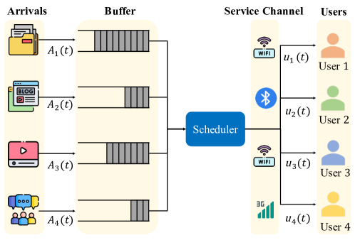
Figure 1: A four-user delay-constrained single-hop network.

We consider the same scheduling problem as in [72, 22, 43], using a four-user example shown in Figure 1. Time is divided into discrete slots, $t\in\{0,1,2,\dots\}$. The scheduler receives job arrivals, such as data packets in a network or parcels at a delivery station, at the beginning of each time slot. The number of job arrivals for user $i$ at time slot $t$ is denoted as $A_{i}(t)$, and we define the arrival vector as $\bm{A}(t)=[A_{1}(t),\dots,A_{N}(t)]$, where $N$ refers to the number of users. Each job for user $i$ has a strict delay constraint $\tau_{i}$, meaning that the job must be served within $\tau_{i}$ slots of its arrival; otherwise, it will become outdated and be discarded.

The Buffer Model

Jobs arriving at the system are initially stored in a buffer, which is modeled by a set of delay-sensitive queues. Specifically, the buffer consists of $N$ separate delay-sensitive queues, one for each user, and each queue has infinite capacity. The state of queue $i$ at time slot $t$ is denoted by $\bm{Q}_{i}(t)=[Q_{i}^{0}(t),Q_{i}^{1}(t),\dots,Q_{i}^{\tau_{i}}(t)]$, where $\tau_{i}$ is the maximum remaining time and $Q_{i}^{\tau}(t)$ represents the number of jobs for user $i$ that have $\tau$ time slots remaining until expiration, for $0\leq\tau\leq\tau_{i}$.

The Service Model

At every time slot $t$, the scheduler makes decisions on the resources allocated to jobs in the buffer. For each user $i$, the decision is denoted as $\bm{v}_{i}(t)=[v_{i}^{0}(t),v_{i}^{1}(t),...,v_{i}^{\tau_{i}}(t)]$, where $v_{i}^{\tau}(t)\in[0,v_{\max}]$ represents the amount of resource allocated to serve each job in queue $i$ with a deadline of $\tau$. Each scheduled job is then passed through a service channel, whose condition is random and represented by $c_{i}(t)$ for user $i$ at time slot $t$. The channel conditions at time slot $t$ are denoted as $\bm{c}(t)=[c_{1}(t),c_{2}(t),...,c_{N}(t)]$. If a job is scheduled but fails in service, it remains in the buffer if it is not outdated. The successful rate to serve each job is jointly determined by the channel condition $c_{i}(t)$ and $\bm{v}_{i}(t)$, i.e., $p_{i}(t)=P_{i}(\bm{v}_{i}(t),c_{i}(t))$.

The Scheduler Objective and Lagrange Dual

For each user $i$, the number of jobs that are successfully served at time slot $t$ is denoted as $u_{i}(t)$. A known weight $\omega_{i}$ is assigned to each user, and the weighted instantaneous throughput is defined as $D(t)=\sum_{i=1}^{N}\omega_{i}u_{i}(t).$ The instantaneous resource consumption at time slot $t$ is denoted as $E(t)=\sum_{i=1}^{N}\bm{v}_{i}^{\top}(t)\bm{Q}_{i}(t),$ and the average resource consumption is $\overline{E}=\lim_{T\to\infty}\frac{1}{T}\sum_{t=1}^{T}E(t)$. The objective of the scheduler is to maximize the weighted average throughput, defined as $\overline{D}=\lim_{T\to\infty}\frac{1}{T}\sum_{t=1}^{T}D(t)$, subject to the average resource consumption limit (corresponds to Equation (1) in [22] and Equation (3) in [43]), i.e.,

$$\mathcal{P}:\max_{\bm{v}_{i}(t):1\leq i\leq N,1\leq t\leq T} \lim_{T\to\infty}\frac{1}{T}\sum_{t=1}^{T}\sum_{i=1}^{N}\omega_{i}u_{i}(t),$$ (1)

s.t. $$\lim_{T\to\infty}\frac{1}{T}\sum_{t=1}^{T}\sum_{i=1}^{N}\bm{v}_{i}^{\top}(t)\bm{Q}_{i}(t)\leq E_{0},$$

where $E_{0}$ is the average resource consumption constraint.

We denote the optimal value of problem $\mathcal{P}$ by $\mathcal{T}^{*}$. Similar to Equation (2) in [22] and Equation (4) in [43], we define a Lagrangian function to handle the average resource budget constraint in problem $\mathcal{P}$, as follows:

$$\mathcal{L}(\pi,\lambda)=\lim_{T\rightarrow\infty}\frac{1}{T}\sum_{t=1}^{T}\sum_{i=1}^{N}\left[\omega_{i}u_{i}(t)-\lambda\bm{v}_{i}^{\top}(t)\bm{Q}_{i}(t)\right]+\lambda E_{0},$$ (2)

where $\pi$ is the control policy and $\lambda$ is the Lagrange multiplier. The policy $\pi$ determines the decision value $\bm{v}_{i}(t)$ explicitly and influences the number of served jobs $u_{i}(t)$ implicitly. We denote $g(\lambda)$ as the Lagrange dual function for a given Lagrange multiplier $\lambda$:

$$g(\lambda)=\max_{\pi}\mathcal{L}(\pi,\lambda)=\mathcal{L}(\pi^{*}(\lambda),\lambda),$$ (3)

where the maximizer is denoted as $\pi^{*}(\lambda)$.

Remark 1.

As shown in [72, 22], the optimal timely throughput, denoted by $\mathcal{T}^{*}$, is equal to the optimal value of the dual problem, i.e., $\mathcal{T}^{*}=\min_{\lambda\geq 0}g(\lambda)=g(\lambda^{*})$, where $\lambda^{*}$ is the optimal Lagrange multiplier. Moreover, the optimal policy $\pi^{*}(\lambda^{*})$ can be obtained by computing the dual function $g(\lambda)$ for some $\lambda$ and applying gradient descent to find the optimal $\lambda^{*}$, as detailed in [72, 22]. According to [22], the derivative of the dual function $g(\lambda)$ is given by $g^{\prime}(\lambda)=\frac{\partial\mathcal{L}(\pi^{*}(\lambda),\lambda)}{\partial\lambda}=E_{0}-E_{\pi^{*}(\lambda)}$, where $E_{\pi^{*}(\lambda)}=\lim_{T\to\infty}\frac{1}{T}\sum_{t=1}^{T}E_{\pi^{*}(\lambda)}(t)$ denotes the average resource consumption under the optimal policy $\pi^{*}(\lambda)$.

We emphasize that, although our formulation builds upon the work of [72, 22], our setting is significantly different. Our goal is to learn an efficient scheduling policy solely from pre-collected data, without interacting with the system. Furthermore, our formulation ensures adherence to resource and delay constraints using the Lagrangian dual and delay-sensitive queues, all in a fully offline manner.

3.1.2 Scalability in Multi-hop Setting

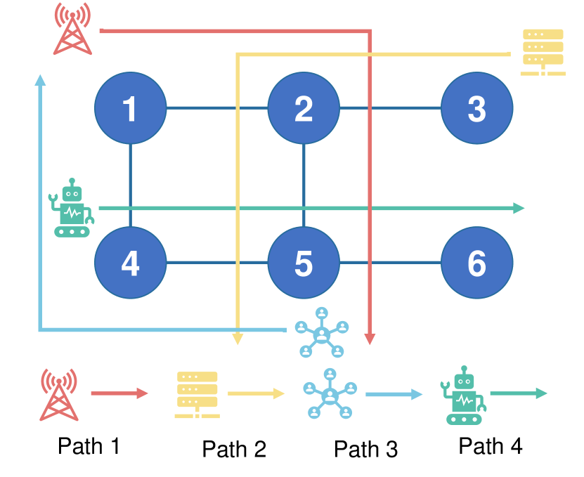
(a) A multi-hop network.

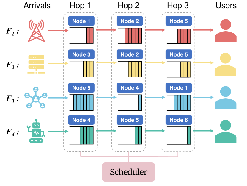
(b) Four aligned flows.

Figure 2: A four-user delay-constrained multi-hop network: (a) The multi-hop network with user flows, and (b) The buffer structure of the network.

We consider a similar multi-hop formulation as in [72, 22, 43]. In a multi-hop network, each data flow spans multiple hops, requiring the scheduler to decide which flows to serve and how to allocate resources at each intermediate node. We consider a multi-hop network consisting of $N$ flows (or users), denoted by $\{F_{1},F_{2},\dots,F_{N}\}$, and $K$ nodes, indexed as $\{1,2,\dots,K\}$. The length of the path for flow $i$ is denoted by $J_{i}$, and the longest path among all flows is given by $J=\max_{1\leq i\leq N}J_{i}$.

The routing of each flow $i$ is encoded in a matrix $\mathbf{H}^{(i)}=(h_{jk}^{(i)})\in\mathbb{R}^{J\times K}$, where $h_{jk}^{(i)}=1$ indicates that the $j$-th hop of flow $i$ corresponds to node $k$, and $h_{jk}^{(i)}=0$ otherwise. At time $t$, the number of jobs arriving for flow $i$ is expressed as $A_{i}(t)$, with each job subject to a strict delay requirement $\tau_{i}$. Furthermore, each node must adhere to an average resource constraint $E_{0}^{(k)}$.

As an example, Figure 2 illustrates a multi-hop network with four distinct flows. These flows traverse the network along the following routes: $F_{1}=\{1\rightarrow 2\rightarrow 5\}$, $F_{2}=\{3\rightarrow 2\rightarrow 5\}$, $F_{3}=\{5\rightarrow 4\rightarrow 1\}$, and $F_{4}=\{4\rightarrow 5\rightarrow 6\}$.

The multi-hop scheduling problem can be viewed as an extension of multiple single-hop scheduling problems, tailored to account for the unique characteristics of multi-hop scenarios. These characteristics include the buffer model, scheduling and service mechanisms, and the overarching system objectives specific to multi-hop networks.

Aggregated Buffer Model

In multi-hop networks, buffers are represented as delay-sensitive queues, similar to those in single-hop networks. However, due to the requirement for jobs to traverse multiple hops to reach their destinations, the buffer model must account for the flow of jobs across the entire network. To effectively describe the system state, we introduce an aggregated buffer model that organizes flows based on their originating nodes, as illustrated in Figure 2.

For a flow $i$ with a path length of $J_{i}$, the buffer state at the $j$-th hop ($1\leq j\leq J_{i}$) is denoted by $\bm{Q}_{i}^{(j)}(t)=[Q_{i}^{(j,0)}(t),Q_{i}^{(j,1)}(t),\dots,Q_{i}^{(j,\tau_{i}-j+1)}(t)]$. Here, $Q_{i}^{(j,\tau)}(t)$ represents the number of jobs in flow $i$ at the $j$-th hop with $\tau$ time slots remaining until expiration, where $0\leq\tau\leq\tau_{i}-j+1$. For hops beyond the path length of flow $i$ ($J_{i}<j\leq J$), the buffer state is set to $\bm{Q}_{i}^{(j)}(t)=\bm{0}$, indicating the absence of flow $i$ in these hops.

This formulation leads to the definition of $J$ aggregated buffers, represented as $\mathbf{Q}^{(1)}(t),\mathbf{Q}^{(2)}(t),\dots,$ $\mathbf{Q}^{(J)}(t)$. Each aggregated buffer $\mathbf{Q}^{(j)}(t)$ consolidates the states of all flows at the $j$-th hop, such that $\mathbf{Q}^{(j)}(t)=[\bm{Q}_{1}^{(j)}(t),\bm{Q}_{2}^{(j)}(t),\dots,\bm{Q}_{N}^{(j)}(t)]$ for $1\leq j\leq J$.

Multi-hop Scheduling and Service Model

At each time slot $t$, the scheduler is responsible for deciding which flows to prioritize and determining the resource allocation for each node. The resources allocated to flow $i$ are represented by $\mathbf{v}_{i}(t)=[\bm{v}_{i}^{(1)}(t),\bm{v}_{i}^{(2)}(t),\dots,\bm{v}_{i}^{(J_{i})}(t)]$, where $\bm{v}_{i}^{(j)}(t)$ specifies the resources assigned to the $j$-th hop of flow $i$, for $1\leq j\leq J_{i}$. Consequently, the complete scheduling decision for all flows at time $t$ is denoted as $\mathbf{V}(t)=[\mathbf{v}_{1}(t),\mathbf{v}_{2}(t),\dots,\mathbf{v}_{N}(t)]$.

Each scheduled job must traverse the service channels along its designated flow path. The service channel condition between nodes $i$ and $j$ at time $t$ is denoted by $c_{ij}(t)$. For a job belonging to flow $i$, given an allocated resource $v$ and channel condition $c$, the probability of successful service is $P_{i}(v,c)$. The instantaneous resource utilization at node $k$ during time slot $t$ is defined as $E^{(k)}(t)=\sum_{i=1}^{N}\sum_{j=1}^{J_{i}}h_{jk}^{(i)}{\bm{v}_{i}^{(j)}}^{\top}(t)\bm{Q}_{i}^{(j)}(t),$ where $h_{jk}^{(i)}$ represents the association of flow $i$’s $j$-th hop with node $k$, and $\bm{Q}_{i}^{(j)}(t)$ denotes the buffer state. The average resource utilization for node $k$ is given by $\overline{E}^{(k)}=\lim_{T\to\infty}\frac{1}{T}\sum_{t=1}^{T}E^{(k)}(t).$

Multi-hop System Objective and Lagrange Dual

The number of jobs successfully served for flow $i$ at time slot $t$ is denoted by $u_{i}(t)$. Each flow is assigned a weight $\omega_{i}$, and the weighted instantaneous throughput is given by $D(t)=\sum_{i=1}^{N}\omega_{i}u_{i}(t)$. The scheduler’s primary objective is to maximize the weighted average throughput, defined as $\overline{D}=\lim_{T\to\infty}\frac{1}{T}\sum_{t=1}^{T}D(t)$, while ensuring compliance with the average resource consumption constraints at each node (similar to Equation (4) in [22]).

$$\mathcal{P}_{m}:\max_{\bm{v}_{i}(t):1\leq i\leq N,1\leq t\leq T} \lim_{T\to\infty}\frac{1}{T}\sum_{t=1}^{T}\sum_{i=1}^{N}\omega_{i}u_{i}(t),$$ (4)

s.t. $$\lim_{T\to\infty}\frac{1}{T}\sum_{t=1}^{T}\sum_{i=1}^{N}\sum_{j=1}^{J_{i}}h_{jk}^{(i)}{\bm{v}_{i}^{(j)}}^{\top}(t)\cdot$$

$$\bm{Q}_{i}^{(j)}(t)\leq E_{0}^{(k)},\quad\forall 1\leq k\leq K,$$

where $E_{0}^{(k)}$ represents the average resource constraint at node $k$. The Lagrangian dual function for the multi-hop optimization problem $\mathcal{P}_{m}$ is expressed as:

$$\mathcal{L}_{m}(\pi,\bm{\lambda})=\lim_{T\to\infty}\frac{1}{T}\sum_{t=1}^{T}\sum_{i=1}^{N}\Big{[}\omega_{i}u_{i}(t)-\sum_{k=1}^{K}\lambda_{k}\sum_{j=1}^{J_{i}}h_{jk}^{(i)}{\bm{v}_{i}^{(j)}}^{\top}(t)\bm{Q}_{i}^{(j)}(t)\Big{]}+\sum_{k=1}^{K}\lambda_{k}E_{0}^{(k)},$$ (5)

where $\bm{\lambda}=[\lambda_{1},\lambda_{2},\dots,\lambda_{K}]$ is the vector of Lagrange multipliers.

The Lagrange dual function, given a fixed multiplier $\bm{\lambda}$, is defined as:

$$g_{m}(\bm{\lambda})=\max_{\pi}\mathcal{L}_{m}(\pi,\bm{\lambda})=\mathcal{L}_{m}(\pi_{m}^{*}(\bm{\lambda}),\bm{\lambda}),$$ (6)

where $\pi_{m}^{*}(\bm{\lambda})$ represents the policy that maximizes the Lagrangian function. To derive the optimal policy $\pi_{m}^{*}(\bm{\lambda}^{*})$, the dual function $g_{m}(\bm{\lambda})$ is optimized using gradient descent to identify the optimal multiplier $\bm{\lambda}^{*}$.

3.1.3 Offline Learning

Although our formulation bears similarities to those in [72, 22, 43], our offline learning-based scheduling setting introduces unique challenges. Specifically, the algorithm cannot interact with the environment during training and must rely entirely on a pre-collected dataset $\mathcal{D}$, which is generated by an unknown behavior policy that governs the data collection process. Importantly, the quality of $\mathcal{D}$ may be limited or suboptimal, as it reflects the biases and imperfections of the behavior policy. The objective, therefore, is to train an effective policy based solely on the dataset, without any online interaction with the system.

3.2 The MDP Formulation

We present the Markov Decision Process (MDP) formulation for our scheduling problem, which allows SOCD to determine the optimal policy $\pi(\lambda)$. Specifically, an MDP is defined by the tuple $\mathcal{M}=\langle\mathcal{S},\mathcal{A},r,\mathbb{P},\gamma\rangle$, where $\mathcal{S}$ represents the state space, $\mathcal{A}$ is the action space, $r$ is the reward function, $\mathbb{P}$ is the transition matrix, and $\gamma$ is the discount factor. The overall system state $\bm{s}_{t}$ includes $\bm{A}(t)$, $\bm{Q}_{1}(t)$, …, $\bm{Q}_{N}(t)$, $\bm{c}(t)$, and possibly other relevant information related to the underlying system dynamics. At each time slot $t$, the action is represented by $\bm{a}_{t}=[\bm{v}_{1}(t),...,\bm{v}_{N}(t)]$. Similar to [43], to take the resource constraint into consideration, we set the reward of the MDP to be

$$r_{t}=D(t)-\lambda E(t),$$ (7)

where $D(t)$ is the instantaneous weighted throughput, and $E(t)$ is the resource consumption weighted by $\lambda$.

The objective of the optimal agent is to learn an optimal policy $\pi(\cdot;\bm{\theta})$, parameterized by $\bm{\theta}$, which maps the state to the action space in order to maximize the expected rewards:

$$J(\pi(\cdot;\bm{\theta}))=\mathbb{E}\left[\sum_{t=0}^{T}\gamma^{t}r(s_{t},a_{t})\mid s_{0},a_{0},\pi(\cdot;\bm{\theta})\right].$$ (8)

Remark 2.

By considering the above MDP formulation, our objective is to maximize the Lagrange function under a fixed $\lambda$, i.e., to obtain the Lagrange dual function in Equation (3). Specifically, the reward setting in Equation (7) implies that when $\gamma=1$, the cumulative discounted reward becomes $R=\sum_{t=1}^{T}\gamma^{t}r_{t}=T{\mathcal{L}}(\pi,\lambda)-\lambda TE_{0}$. Therefore, an algorithm that maximizes the expected rewards $J(\pi(\cdot;\phi))$ also maximizes the Lagrangian function, which is the objective of SOCD as detailed in Section 4. Furthermore, we emphasize that our goal is to learn an efficient scheduling policy based purely on pre-collected data without interacting with the system.

4 SOCD: Offline RL-based Scheduling

This section provides a comprehensive description of SOCD, our offline RL-based scheduling algorithm. The SOCD framework comprises two fundamental components designed to address offline scheduling tasks: the critic-guided diffusion policy for offline reinforcement learning (Section 4.1) and the Lagrange multiplier optimization (Section 4.2). The overall structure of the proposed SOCD algorithm is depicted in Figure 3.

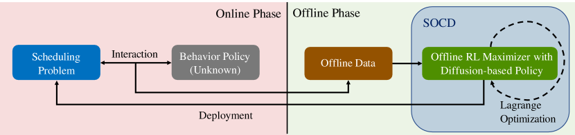
Figure 3: The SOCD algorithm: Operating solely in the offline phase, it does not require online interactions or prior knowledge of system dynamics. This makes it particularly well-suited for scenarios where online system interactions are either impractical or infeasible.

4.1 Offline RL Maximizer with Diffusion-based Policy

In this subsection, we introduce our offline reinforcement learning (RL) algorithm, which consists of two key components: a diffusion model for behavior cloning and a critic model for learning the state-action value function (Q-value). The primary objective is to maximize the Lagrangian function in Equation (3) for a fixed Lagrange multiplier $\lambda$, without requiring online interactions.

We begin by considering the general offline RL setting, where the Markov Decision Process (MDP) is defined as $\langle\mathcal{S},\mathcal{A},r,\mathbb{P},\gamma\rangle$, and the offline dataset $\mathcal{D}^{\mu}=\left\{\mathcal{T}_{j}=(\bm{s}^{j}_{1},\bm{a}^{j}_{1},\dots,\bm{s}^{j}_{t},\bm{a}^{j}_{t},\dots,\bm{s}^{j}_{T},\bm{a}^{j}_{T})\right\}_{j=1}^{J}$ is collected by a behavior policy $\mu(\cdot|\bm{s})$. We define the state-action value function (i.e., the critic model) as $Q(\bm{s},\bm{a})$ and the policy as $\pi(\cdot|\bm{s})$.

To ensure the learned policy remains close to the behavior policy while maximizing the expected value of the state-action functions, prior work [62, 55] has explicitly constrained the policy $\pi$ using the following formulation:

$$\mathop{\mathrm{arg\ max}}_{\pi}\quad\int_{\mathcal{S}}\rho_{\mu}(\bm{s})\int_{\mathcal{A}}\pi(\bm{a}|\bm{s})Q(\bm{s},\bm{a})\mathrm{d}\bm{a}\mathrm{d}\bm{s}-\frac{1}{\alpha}\int_{\mathcal{S}}\rho_{\mu}(\bm{s})D_{\mathrm{KL}}\left(\pi(\cdot|\bm{s})||\mu(\cdot|\bm{s})\right)\mathrm{d}\bm{s}.$$ (9)

Here, $\rho_{\pi}(\bm{s})=\sum_{n=0}^{\infty}\gamma^{n}p_{\pi}(\bm{s}_{n}=\bm{s})$ denotes the discounted state visitation frequencies induced by policy $\pi$, with $p_{\pi}(\bm{s}_{n}=\bm{s})$ representing the probability of the event $\{\bm{s}_{n}=\bm{s}\}$ under policy $\pi$. The optimal policy $\pi^{*}$ of Equation (9) can be derived using the method of Lagrange multipliers [62, 55]:

$$\pi^{*}(\bm{a}|\bm{s}) =\frac{1}{Z(\bm{s})}\mu(\bm{a}|\bm{s})\mathrm{exp}\left(\alpha Q(\bm{s},\bm{a})\right),$$ (10)

where $Z(\bm{s})$ is the partition function and $\alpha$ is he temperature coefficient.

A key observation based on Equation (10) is that $\pi^{*}$ can be decoupled into two components: (1) a behavior cloning (BC) model $\mu_{\bm{\theta}}(\cdot|\bm{s})$ trained on $\mathcal{D}^{\mu}$ parameterized by $\bm{\theta}$, which is irrelevant to the Lagrange multiplier $\lambda$, and (2) a critic model $Q_{\bm{\phi}}(\bm{s},\bm{a})$ parameterized by $\bm{\phi}$, which is influenced by the Lagrange multiplier $\lambda$.

4.1.1 Diffusion-based Behavior Cloning

It is critical for the BC model to express multi-modal action distributions, as previous studies [83, 7] have pointed out that uni-modal policies are prone to getting stuck in suboptimalities. Moreover, offline RL methods often suffer from value overestimation due to the distributional shift between the dataset and the learned policy [36], underscoring the importance of maintaining high fidelity in the BC model. To address these challenges, we propose cloning the behavior policy using diffusion models, which have demonstrated significant success in modeling complex and diverse distributions [65].

We adopt the score-based structure introduced in [76]. To be specific, the forward process of the diffusion model gradually adds Gaussian noise to the action distribution conditional on the state given by the behavior policy, i.e., $p_{0}(\bm{a}_{0}|\bm{s})=\mu(\bm{a}_{0}|\bm{s})$, such that the conditional transition function is given by $p_{t0}(\bm{a}_{t}|\bm{a}_{0},\bm{s})=\mathcal{N}(\bm{a}_{t};\alpha_{t}\bm{a}_{0},\sigma_{t}^{2}\bm{I})$ for some $\alpha_{t},\sigma_{t}>0$ and with a sufficiently small $\alpha_{T}$, $p_{T0}(\bm{a}_{T}|\bm{a}_{0},\bm{s})\approx\mathcal{N}(\bm{a}_{T};0,\bm{I})$. This corresponds to a stochastic differential equation (SDE) $\mathrm{d}\bm{a}_{t}=f(\bm{a}_{t},t)\mathrm{d}t+g(t)\mathrm{d}\bm{w}_{t}$, where $\bm{w}_{t}$ is a standard Wiener process and $f(\cdot,t)$, $g(t)$ are called drift coefficient and diffusion coefficient, respectively [76]. Following the Variance Preserving (VP) SDE setting as introduced in [76], we choose $\alpha_{t}=e^{-\frac{1}{2}\int_{0}^{t}\omega(s)\mathrm{d}s}$ and $\sigma_{t}^{2}=1-e^{-\int_{0}^{t}\omega(s)\mathrm{d}s}$, where $\omega(t)=\left(\omega_{\max}-\omega_{\min}\right)t+\omega_{\min}$ such that $f(\bm{a}_{t},t)=\bm{a}_{t}\frac{{\rm{d}}\log\alpha_{t}}{{\rm{d}}t}$, $g^{2}(t)=\frac{{\rm{d}}\sigma_{t}^{2}}{{\rm{d}}t}-2\frac{{\rm{d}}\log\alpha_{t}}{{\rm{d}}t}\sigma_{t}^{2}$.

Based on the findings in [76, 30], a corresponding reverse stochastic differential equation (SDE) process exists, enabling the transition from $T$ to $0$ that guarantees that the joint distribution $p_{0:T}(\bm{a}_{0},\bm{a}_{1},...,\bm{a}_{T})$ are consistent with the forward SDE process. This process is detailed in Equation (2.4) of [48] that considers the state $\bm{s}$ as conditioning variables:

$${\rm{d}}\bm{a}_{t}=\big{[}f(\bm{a}_{t},t)-g^{2}(t)\underbrace{\nabla_{\bm{a}_{t}}p_{t}(\bm{a}_{t}|\bm{s})}_{\text{Neural Network }\bm{s}_{\bm{\theta}}}\big{]}{\rm{d}}t+g(t){\rm{d}}\overline{\bm{w}}_{t},$$ (11)

where $p_{t}(\bm{a}_{t}|\bm{s})=\int_{\bm{a_{0}}}p_{t0}(\bm{a}_{t}|\bm{a}_{0},\bm{s})\mu(\bm{a}_{0}|\bm{s}){\rm{d}}\bm{a}_{0}$ is the state-conditioned marginal distribution of $\bm{a}_{t}$ including the unknown data distribution $\mu$, and $\overline{\bm{w}}_{t}$ represents a standard Wiener process when time flows backwards from $T$ to $0$.

To fully characterize the reverse SDE process described in Equation (11), it is essential to obtain the conditional score function, defined as $\nabla_{\bm{a}_{t}}p_{t}(\bm{a}_{t}|\bm{s})$, at each $t$. The score-based model is to learn the conditional score model $\mathbf{s}_{\bm{\theta}}(\bm{a}_{t},\bm{s},t)$ that estimates the conditional score function of the behavior action distribution by minimizing the score-matching objective [76]:

$$\mathcal{L}(\bm{\theta})=\mathbb{E}_{(\bm{s},\bm{a})\sim D^{\mu},\bm{\epsilon},t}[\|\sigma_{t}\mathbf{s}_{\bm{\theta}}(\alpha_{t}\bm{a}+\sigma_{t}\bm{\epsilon},\bm{s},t)+\bm{\epsilon}\|_{2}^{2}],$$ (12)

where $\bm{\epsilon}\sim\mathcal{N}(0,\bm{I})$, $t\sim\mathcal{U}(0,T)$. When sampling, the reverse process of the score-based model solves a diffusion ODE from time $T$ to time $0$ to obtain $\bm{a}_{0}\sim\mu_{\bm{\theta}}(\cdot|\bm{s})$:

$$\mathrm{d}\bm{a}_{t}=\bigg{[}f(\bm{a}_{t},t)-\frac{1}{2}g^{2}(t)\mathbf{s}_{\bm{\theta}}(\bm{a}_{t},\bm{s},t)\bigg{]}\mathrm{d}t.$$ (13)

with $\bm{a}_{T}$ sampled from $\mathcal{N}(0,\bm{I})$. In this manner, we can effectively perform behavior cloning using a diffusion policy.

It is important to note that training the diffusion policy is independent of the Lagrange multiplier $\lambda$, which means that the policy only needs to be trained once compared with other offline RL-based scheduling algorithm, e.g., SOLAR [43] needs multiple iterations of the policy for different Lagrange multiplier $\lambda$. This significantly enhances the model’s reusability and reduces training time.

4.1.2 Sampling-free Critic Learning

The objective of training the state-action value function $Q_{\bm{\phi}}(\bm{s},\bm{a})$ is to minimize the temporal difference (TD) error under the Bellman operator, which is expressed as:

$$\mathcal{L}(\bm{\phi})= \mathbb{E}_{(\bm{s},\bm{a},\bm{r},\bm{s}^{\prime})\sim\mathcal{D}^{\mu},\bm{a}^{\prime}\sim\pi(\cdot|\bm{s}^{\prime})}\left[(\gamma\min_{k=1,2}Q_{\overline{\bm{\phi}}}^{k}(\bm{s}^{\prime},\bm{a}^{\prime})+\bm{r}-Q_{\bm{\phi}}(\bm{s},\bm{a}))^{2}\right].$$ (14)

Nevertheless, calculating the TD loss requires generating new (and potentially unseen) actions $\bm{a}^{\prime}$, which is computationally inefficient, especially when relying on multiple steps of denoising under diffusion sampling. Additionally, generating out-of-sample actions introduces potential extrapolation errors [17], which can degrade the quality of value estimates.

To address these challenges, we propose a sampling-free approach for training the critic by directly using the discounted return as the target. Specifically, for each trajectory $\mathcal{T}=(\bm{s}_{1},\bm{a}_{1},\bm{r}_{1},\dots,\bm{s}_{t}$ $,\bm{a}_{t},\bm{r}_{t},\dots,\bm{s}_{T},\bm{a}_{T},\bm{r}_{T})$ with rewards calculated via Equation (7), which is randomly sampled from the offline dataset $\mathcal{D}^{\mu}$, we define the critic’s training objective as:

$$\mathcal{L}(\bm{\phi})=\mathbb{E}_{t\sim\mathcal{U}(1,T),\mathcal{T}\sim\mathcal{D}^{\mu}}\left[(\min_{k=1,2}Q_{\bm{\phi}}^{k}(\bm{s}_{t},\bm{a}_{t})-\sum_{i=t}^{T}\gamma^{i-t}\bm{r}_{i})^{2}\right].$$ (15)

By incorporating the double Q-learning technique [20], this approach ensures stable loss convergence during training. Additionally, it helps mitigate the overestimation bias in Q-value estimation, leading to consistently strong performance during evaluation. The proposed method has shown to be both robust and computationally efficient, making it a reliable strategy for training the critic in offline RL settings.

4.1.3 Selecting From Samples

We can generate the final output action from the trained BC model (diffusion policy) under the guidance of the trained critic model. The action-generation procedure is shown in Algorithm 1.

According to Equation (10), for a given state $\bm{s}$, we can generate the action $\bm{a}^{\prime}\sim\pi^{*}(\cdot|\bm{s})$ using importance sampling. Specifically, $K$ actions $\{\bm{a}^{(k)}_{0}\}_{k=1}^{K}$ are sampled using the diffusion-based BC model $\mu_{\bm{\theta}}(\cdot|\bm{s})$ (Line 3, Line 4). The final action $\bm{a}^{\prime}\sim\pi^{*}(\cdot|\bm{s})$ is then obtained by applying the importance sampling formula (Line 7):

$$\bm{a}^{\prime}=\sum_{k=1}^{K}\frac{\mathrm{exp}\left(\alpha Q_{\bm{\phi}}(\bm{s},\bm{a}^{(k)}_{0})\right)}{\sum_{k=1}^{K}\mathrm{exp}\left(\alpha Q_{\bm{\phi}}(\bm{s},\bm{a}^{(k)}_{0})\right)}\bm{a}^{(k)}_{0}.$$ (16)

This formula computes a weighted combination of actions $\bm{a}^{(k)}_{0}$ based on their Q-values $Q_{\phi}(\bm{s},\bm{a}^{(k)}_{0})$, where $\alpha$ is the temperature coefficient that governs the trade-off between adhering to the behavior policy and selecting actions that are more likely to yield higher rewards according to the Q-value function.

Empirically, we observe that selecting the action with the maximum Q-value across the sampled actions (which corresponds to $\alpha=+\infty$) provides more stable performance in many scenarios (Line 7). This is formalized as:

$$\bm{a}^{\prime}=\mathop{\mathrm{argmax}}_{\bm{a}^{(k)}_{0}}Q_{\bm{\phi}}(\bm{s},\bm{a}^{(k)}_{0})$$ (17)

which involves simply choosing the action with the highest Q-value among the $K$ sampled actions. This approach simplifies the selection process while still leveraging the value function to select high-reward actions.

In both scenarios, our final action is essentially a weighted combination of the actions output by the BC model, which leverages the expressivity and generalization capability of the diffusion model while significantly reducing extrapolation errors introduced by out-of-distribution actions generated.

Note that a larger value of $K$ offers distinct advantages. In the importance sampling case, increasing $K$ improves the approximation of the target distribution $\pi^{*}(\cdot|\bm{s})$. In the case of selecting the action with the maximum Q-value, a larger $K$ provides a broader set of options, thus increasing the likelihood of selecting the optimal action. Therefore, we use the DPM-solver [48] as the sampler to enhance sampling efficiency, enabling support for a larger value of $K$.

Algorithm 1 Scheduling By Offline Learning with Critic Guidance and Diffusion Generation ($\mathtt{SOCD}$) (Action Generation)

1: Input: State $\bm{s}$, BC model $\mu_{\bm{\theta}}$, Q-networks $Q_{\bm{\phi}}^{1},Q_{\bm{\phi}}^{2}$ // Input Trained Model and Current State

2: for Behavior sampling step $k=1$ to $K$ do

3:  Sample $\bm{a}^{(k)}_{T}$ from $\mathcal{N}(0,\bm{I})$. // Sampling Raw Noise

4:  Sample $\bm{a}^{(k)}_{0}$ from BC model $\mu_{\bm{\theta}}(\cdot|\bm{s})$ by solving Equation (13). // Diffusion Generation

5:  Calculate the Q-value for action $\bm{a}^{(k)}_{0}$: $Q_{\bm{\phi}}(\bm{s},\bm{a}^{(k)}_{0})=\min_{k=1,2}Q_{\bm{\phi}}^{k}(\bm{s},\bm{a}^{(k)}_{0})$. // Critic Guidance

6: end for

7: Obtain final action $\bm{a}^{\prime}$ via Equation (16) (Importance Sampling) or (17) (Argmax Selecting). // Obtain Final Action

8: Output: Final action $\bm{a}^{\prime}$

4.1.4 User-level Decomposition

In the MDP of multi-user scheduling systems, the dimensionality of the input state and action spaces scales with the number of users, which poses a considerable challenge to learning in large-scale scenarios due to the restricted capacity of the neural networks used for learning policies.

To address this limitation, we adopt the user-level decomposition techniques introduced in [22]. Specifically, we decompose the original MDP into $N$ user-specific sub-MDPs. For each user $i$, the state is $\bm{s}_{t}^{(i)}=[i,A_{i}(t),\bm{Q}_{i}(t),c_{i}(t)]$, the action is $\bm{a}_{t}^{(i)}=\bm{v}_{i}(t)$, and the reward becomes $\bm{r}_{t}^{(i)}=\omega_{i}u_{i}(t)-\bm{v}_{i}^{T}(t)\bm{Q}_{i}(t)$ at each time slot $t$.

By introducing an additional user index $i$ into the state representation of each sub-MDP, we can train a single model that generates actions for all users. This approach reduces the complexity of the problem by keeping the dimensionality of the input states and actions constant, regardless of the number of users. Consequently, this decomposition enhances the scalability of the algorithm, allowing it to efficiently handle larger multi-user systems.

4.2 Lagrange Optimization via Offline Data

To ensure the resource constraint, SOCD adopts a Lagrangian dual method. According to Remark 1, for a given $\lambda$ value, the gradient of the dual function with respect to $\lambda$ is:

$$g^{\prime}(\lambda)=\frac{\partial\mathcal{L}(\pi^{*}(\lambda),\lambda)}{\partial\lambda}=E_{0}-E_{\pi^{*}(\lambda)}.$$ (18)

Here $E_{\pi^{*}(\lambda)}$ is the groundtruth average resource consumption under the policy $\pi^{*}(\lambda)$. Thus, we can update the Lagrange multiplier $\lambda$ according to:

$$\lambda\leftarrow\lambda-\alpha g^{\prime}(\lambda)=\lambda-\alpha(E_{0}-E_{\pi^{*}(\lambda)}).$$ (19)

Then, after updating the value of $\lambda$, we modify the offline dataset’s reward using $r_{t}=D(t)-\lambda E(t)$ and iterate the learning procedure.

While our method is similar to that in [22], the offline learning nature means that we cannot learn the value $E_{\pi^{*}(\lambda)}$ by interacting with the environment, as is done in online algorithms [22].

To address the problem of estimating $E_{\pi^{*}(\lambda)}$, we propose to estimate the resource consumption in an offline manner. Specifically, given a fixed $\lambda$, we train the algorithm and obtain a policy. Then, we sample $n$ trajectories $\{\mathcal{T}_{j}\}_{j=1}^{n}$ from the dataset $\mathcal{D}$. For each trajectory $\mathcal{T}_{j}=(\bm{s}^{j}_{1},\bm{a}^{j}_{1},...\bm{s}^{j}_{t},\bm{a}^{j}_{t},...,\bm{s}^{j}_{T},\bm{a}^{j}_{T})$, we feed the states $\bm{s}^{j}_{t}$ into the network, and obtain the output action $\hat{\bm{a}}^{j}_{t}=[\hat{\bm{v}}^{j}_{1}(t),...,\hat{\bm{v}}^{j}_{N}(t)]\sim\pi_{\bm{\theta}}(\cdot|\bm{s}^{j}_{t})$. According to (3.1.1), the resource consumption is estimated as $\hat{E}^{j}_{t}=\sum_{i=1}^{N}\hat{\bm{v}}^{j}_{i}(t)^{\top}\bm{Q}^{j}_{i}(t)$. Here $\bm{Q}^{j}_{i}(t)$ is the buffer information included in $\bm{s}_{t}^{j}$. Thus, the average resource consumption over the sampled trajectories can be given as

$$\hat{E}_{\pi^{*}(\lambda)}=\frac{1}{n}\sum_{j=1}^{n}\frac{1}{T}\sum_{t=1}^{T}\hat{E}^{j}_{t}.$$ (20)

We use Equation (20) as an estimate for $E_{\pi^{*}(\lambda)}$. This approach effectively avoids interacting with the environment and enables an offline estimation of $E_{\pi^{*}(\lambda)}$. Note that if the policy is allowed to interact with the environment, we can evaluate the policy of SOCD in the online phase to obtain the groundtruth value of $E_{\pi^{*}(\lambda)}$ and update the Lagrange multiplier more accurately. However, in the offline phase, it is impossible to acquire the accurate value.

The pseudocode for the SOCD algorithm is shown in Algorithm 2. Our algorithm provides a systematic way to integrate the offline RL algorithm to solve the offline network scheduling problems. The novelty of the algorithm lies in two key aspects: First, SOCD integrates a diffusion-based scheduling policy into the framework, leveraging its superior performance in general offline RL tasks [9]. Second, SOCD requires training the behavioral cloning (BC) model, specifically the diffusion policy, only once in the offline scheduling task. This design significantly enhances training efficiency compared to baseline algorithms such as SOLAR [43], which necessitate multiple policy training iterations following each update of the Lagrange multiplier.

Algorithm 2 Scheduling By Offline Learning with Critic Guidance and Diffusion Generation ($\mathtt{SOCD}$) (Training)

1: Input: Dataset $\mathcal{D}$, initialize Diffusion-based BC model $\mu_{\bm{\theta}}$ with random parameter $\bm{\theta}$ // BC Model Initialization

2: for BC training step $b=1$ to $S$ do

3:  Sample a random minibatch of $\mathcal{B}\times T$ state-action Pairs $(\bm{s},\bm{a})$ from dataset $\mathcal{D}$. // Sampling State-action pairs

4:  Update BC Model $\mu_{\bm{\theta}}$ to minimize (12). // Update BC Model

5: end for

6: for Lagrange multiplier iteration step $k=1,...,K$ do

7:  Input: Initialize Q-networks $Q_{\bm{\phi}}^{1},Q_{\bm{\phi}}^{2}$, policy network $\pi$ with random parameters $\bm{\phi}^{1},\bm{\phi}^{2}$, target Q-networks with $\overline{\bm{\phi}}^{1}\leftarrow\bm{\phi}^{1},\overline{\bm{\phi}}^{2}\leftarrow\bm{\phi}^{2}$, Lagrange multiplier $\lambda$. // Critic Initialization

8:  for training step $i=1$ to $T$ do

9:   Sample a random minibatch of $\mathcal{B}$ trajectories $\left\{\mathcal{T}_{j}=(\bm{s}^{j}_{1},\bm{a}^{j}_{1},\bm{r}^{j}_{1},...\bm{s}^{j}_{t},\bm{a}^{j}_{t},\bm{r}^{j}_{t},...,\bm{s}^{j}_{T},\bm{a}^{j}_{T},\bm{r}^{j}_{T})\right\}_{j=1}^{\mathcal{B}}$ from dataset $\mathcal{D}$ with reward updated (${r}=E-\lambda D$). // Sampling Trajectories

10:   Update critics $\bm{\phi}^{1},\bm{\phi}^{2}$ to minimize (15). // Update Critic

11:   Update target networks: $\overline{\bm{\phi}}^{k}\leftarrow\rho\bm{\phi}^{k}+(1-\rho)\overline{\bm{\phi}}^{k}$,$(k=1,2)$. // Soft Update Target Critic

12:  end for

13:  With action-generation procedure (Algorithm 1), obtain the value $\hat{E}_{\pi^{*}(\lambda)}$ via (20) and update $\lambda$ via (19). // Update Lagrange Multiplier

14: end for

5 Experimental Results

We evaluate SOCD in numerically simulated environments. Section 5.1 details the experimental setup and the properties of the offline dataset. Section 5.2 describes the network architecture and provides the hyperparameter configurations. In Sections 5.3 and 5.4, we introduce several baseline scheduling algorithms known for their effectiveness, and compare SOCD’s performance against them in both standard and more demanding offline scheduling scenarios.

5.1 Environment Setup

This subsection specifies the setup of the delay-constrained network environments, as depicted in Figure 1, where our experiments are conducted. We employ a setup similar to existing works [72, 8, 22], where each interaction step corresponds to a single time slot in the simulated environment. A total of $T=100$ interaction steps (or time steps) define one episode during data collection and training. Each episode is represented by the data sequence $(\bm{s}_{0},\bm{a}_{0},\dots,\bm{s}_{T},\bm{a}_{T})$. In addition, we perform online algorithm evaluations over 20 rounds, each consisting of 1000 time units of interaction with the environment, to ensure accuracy and reliability.

To showcase SOCD’s superior performance across varying system dynamics, we conduct experiments in a variety of diverse environments. The specific settings for all environments used in our experiments are detailed in Table 1 and Table 2.

Table 1: Environment Information: The table outlines various environment configurations used in this study. “Poisson” refers to a Poisson arrival process and Markovian channel conditions, while “Real” refers to environments based on real records. “-$x$hop” indicates the number of hops in the network, while “-$x$user” denotes the number of users in the environment (without this flag the default is 4 users). “-partial” signifies the presence of partial information in the environment.

Environment	User	Flow Generation	Channel Condition	Hop	Partial
Poisson-1hop	4	Poisson	Markovian	1	False
Poisson-2hop	4	Poisson	Markovian	2	False
Poisson-3hop	4	Poisson	Markovian	3	False
Poisson-100user	100	Poisson	Markovian	1	False
Real-1hop	4	Real Record	Real Record	1	False
Real-2hop	4	Real Record	Real Record	2	False
Real-partial	4	Real Record	Real Record	1	True

Table 2: Environment Information Continued. The environment characteristics follow the same explanation as in Table 1.

Environment	Delay $\tau$	Weight $\omega_{i}$	Instantaneous Arrival Rate
Poisson-1hop	[4, 4, 4, 6]	[4, 2, 1, 4]	[3, 2, 4, 2]
Poisson-2hop	[5, 5, 5, 7]	[4, 2, 1, 4]	[3, 2, 4, 2]
Poisson-3hop	[6, 6, 6, 8]	[4, 2, 1, 4]	[3, 2, 4, 2]
Poisson-100user	$[3.39\pm 1.75]^{100}$	$[3.09\pm 1.46]^{100}$	$[3.64\pm 1.18]^{100}$
Real-1hop	[2, 5, 1, 3]	[1, 4, 4, 4]	/
Real-2hop	[3, 6, 2, 4]	[1, 4, 4, 4]	/
Real-partial	[2, 5, 1, 3]	[1, 4, 4, 4]	/

5.1.1 Arrivals and Channel Conditions

The arrivals and channel conditions are modeled in two distinct ways: (1) The arrivals follow the Poisson processes, while the channel conditions are assumed to be Markovian. (2) The arrivals are based on trajectories with various types from an LTE dataset [46], which records the traffic flow of mobile carriers’ 4G LTE network over the course of approximately one year. The channel conditions are derived from a wireless 2.4GHz dataset [79], which captures the received signal strength indicator (RSSI) in the check-in hall of an airport.

5.1.2 Outcomes

We adopt the same assumption for the probability of successful service as proposed in [8, 22]. Specifically, the probability of successful service for user $i$, given channel condition $c$ and allocated resource $v$ is modeled as follows:

$$P_{i}(v,c)=\frac{2}{1+\exp\left(-\frac{2v}{l_{i}^{3}c}\right)}-1,$$ (21)

where $l_{i}$ denotes the distance between user $i$ and the server. This model is representative of a wireless downlink system, where $v$ is interpreted as the transmission power of the antenna responsible for transmitting the current packet [8].

5.1.3 Offline Dataset

We set the episode length to $T=100$. Each dataset comprises $J=5000$ episodic trajectories, generated using the online RSD4 algorithm [22]. During the training procedure of RSD4, the algorithm interacts with the environment to generate new trajectories, which are then stored in the replay buffer for training purposes. We retain the first $5000$ trajectories from the RSD4 replay buffer to form the offline dataset. Details of this dataset are provided in Table 3, all of which are of medium quality, i.e., generated by a suboptimal behavior policy.

Table 3: Dataset Information. The environment characteristics follow the same explanation as in Table 1. L.R. refers to the Learning Rate.

Environment	RSD4 L.R.	$\lambda$ under RSD4	Throughput	Resource Consumption
Poisson-1hop	0.0001	1.0	12.77$\ \pm\$1.14	14.64$\ \pm\$4.47
Poisson-2hop	0.0001	0.5	9.52$\ \pm\$1.44	15.71$\ \pm\$4.61
Poisson-3hop	0.0001	0.001	1.62$\ \pm\$0.44	25.90$\ \pm\$2.27
Poisson-100user	0.0003	0.1	53.55$\ \pm\$4.12	356.46$\ \pm\$102.83
Real-1hop	0.0001	1.0	5.84$\ \pm\$1.56	6.70$\ \pm\$2.54
Real-2hop	0.0001	0.1	0.56$\ \pm\$0.47	5.26$\ \pm\$4.13
Real-partial	0.0001	1.0	5.94$\ \pm\$1.23	5.60$\ \pm\$1.63

5.2 Network Structures and Hyperparameters

For the score model $\mathbf{s}_{\bm{\theta}}(\cdot,\bm{s},t)$ used in the diffusion-based behavior cloning (BC) component of our SOCD algorithm as defined in Equation (11) , we embed the time slot $t$ via Gaussian Fourier Projection [66], resulting in a latent representation of dimension 32, while the state $\bm{s}$ is embedded as a latent variable of dimension 224. These embeddings are concatenated and subsequently passed through a 4-layer multi-layer perceptron (MLP) with hidden layer sizes of $[512,256,256,256]$, using the SiLU activation function [67]. For the critic model, we employ a 2-layer MLP with 256 hidden units and ReLU activation. The hyperparameters of the SOCD algorithm are detailed in Table 4.

Table 4: Hyperparameter Information.

Hyperparameter	Value
BC Model Training Steps	$1\times 10^{5}$
BC Model Learning Rate	$1\times 10^{-4}$
BC Model Optimizer	Adam
Critic Training Steps	$3\times 10^{3}$
Critic Learning Rate	$3\times 10^{-4}$
Critic Optimizer	Adam
Soft Update Parameter $\rho$	$0.05$
Discount Factor $\gamma$	$0.8$
Temperature Coefficient $\alpha$	$100$
DPM-solver Sampling Steps	$10$
Number of Behavior Actions sampled per state	$1024$
$\omega_{min}$	0.1
$\omega_{max}$	20
Batch Size $\mathcal{B}$	50

The network architecture and hyperparameters for the SOLAR algorithm used in this study are consistent with those presented in [43].

5.3 Baselines

We compare our SOCD algorithm with several alternative algorithms, including the offline DRL algorithm Behavior Cloning (BC) [37], a DRL-based scheduling algorithm SOLAR [43], and traditional scheduling methods including Uniform and Earliest Deadline First (EDF) [14], as described below. Note that while there exist other online DRL algorithms, e.g., RSD4 [22], they require online interaction and are thus not suitable for the offline learning setting. We also exclude the programming-type methods from our baselines, as they requires access to full environment information, whereas in the offline setting, dynamic information is completely unavailable.

Behavior Policy

We compare the performance with that of the behavior policy, which is represented by the average score of all trajectories in the offline dataset.

Uniform

This method allocates available resources uniformly across all packets in the buffer, without considering their individual characteristics or deadlines.

Earliest Deadline First (EDF)

The EDF algorithm prioritizes packets based on the remaining time to their respective deadlines [14]. Specifically, it serves packets with the shortest remaining time to deadline first, assigning the maximum available resource allocation, $e_{max}$, to these packets. The process is repeated for packets with the next smallest remaining time to deadline, continuing until the total resource allocation reaches the hard limit $E_{0}$.

Behavior Cloning (BC)

The Behavior Cloning method aims to learn a policy network by minimizing the following objective [37]:

$$\mathcal{L}(\theta)=\mathbb{E}_{(\bm{s},\bm{a})\sim\mathcal{D},\tilde{\bm{a}}\sim\pi_{\theta}(\cdot|\bm{s})}\left[(\tilde{\bm{a}}-\bm{a})^{2}\right].$$ (22)

This objective strives to imitate the behavior policy by reducing the discrepancy between the actions predicted by the policy network and the actions observed in the dataset. In our experiments, we leverage the diffusion-based BC model within our SOCD algorithm to evaluate the performance of the Behavior Cloning approach.

SOLAR

SOLAR is a scheduling algorithm based on offline reinforcement learning [43], where the RL maximizer is an actor-critic RL framework. The critic is trained using a conservative regularized loss function, while the actor loss incorporates Actor Rectification [57] technique, as detailed in [43]. Although both SOLAR and our SOCD algorithm share the same framework, comprising an offline RL maximizer and Lagrange multiplier optimization, SOLAR exhibits inferior performance compared to SOCD. This performance is primarily due to the higher fidelity and the expressivity provided by the diffusion model within SOCD, as demonstrated in the results below.

5.4 Performance Evaluation

To demonstrate the effectiveness of SOCD, we evaluate its performance across a diverse set of environments, as summarized in Table 1. These environments are carefully designed to capture a broad range of challenges, including single-hop and multi-hop network configurations, both simulated and real-world arrival and channel conditions, settings with full and partial observability, as well as large-scale environments that test the scalability and robustness of the proposed method. In the following sections, we present and discuss the results in detail.

5.4.1 Single-hop Environments

We begin by evaluating the performance in a single-hop environment, where both arrivals and channel conditions are modeled as Poisson processes, as denoted by Poisson-1hop in Table 1.

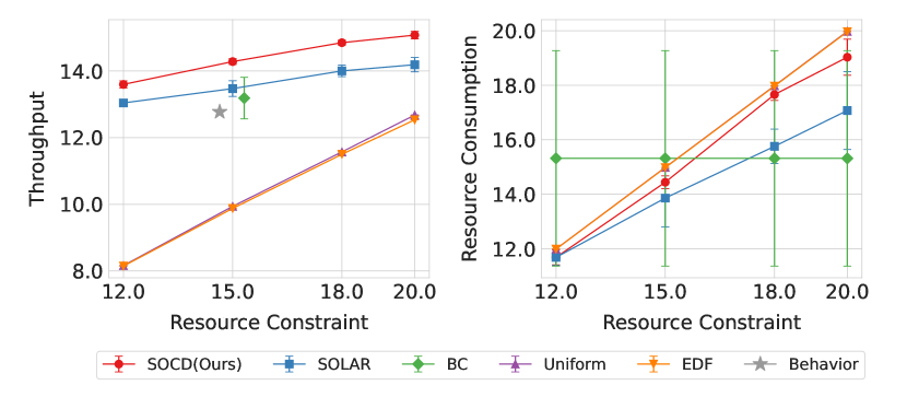
Figure 4: Comparison of different algorithms in the Poisson-1hop environment, where arrivals and channel conditions are modeled as Poisson processes. The plots display throughput (left) and resource consumption (right) under varying resource constraints.

The results are shown in Figure 4. The Behavior Cloning (BC) policy consistently exhibits the same variance because its training relies solely on the state and action data from the dataset, without incorporating the reward signal which includes the Lagrange multiplier. As a result, its outcomes remain unaffected by resource constraints.

The results demonstrate that SOCD effectively learns an efficient policy, outperforming traditional scheduling methods, such as Uniform and EDF. Additionally, both SOCD and SOLAR outperform the behavior policy, indicating that DRL-based algorithms can successfully generalize beyond the suboptimal behavior policy embedded in the offline dataset to effectively utilize the offline data to learn improved policies. Notably, SOCD consistently outperforms SOLAR in terms of both throughput and resource consumption efficiency, further highlighting the superiority of SOCD.

5.4.2 Multi-hop Environments

We extend the evaluation to multi-hop settings, starting with Poisson-2hop, a 2-hop network environment where arrivals and channel conditions are modeled as Poisson processes.

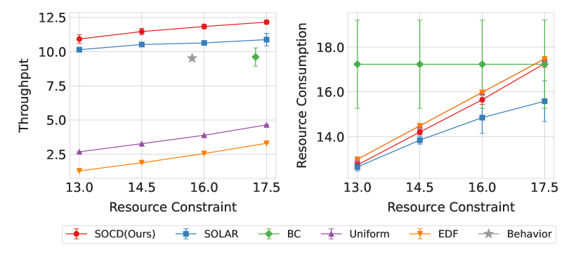
Figure 5: Comparison of different algorithms in a 2-hop environment, Poisson-2hop, with arrivals and channel conditions modeled as Poisson processes. The left column shows throughput, while the right column illustrates resource consumption under varying resource constraints.

As shown in Figure 5, SOCD outperforms SOLAR, further demonstrating its robustness in optimizing scheduling policies across different network topologies. A noteworthy point is that the BC policy and the behavior policy exhibit significantly different performance, suggesting that the learned behavior policy can diverge from the average policy observed in the offline dataset due to the diversity in actual behavior. Despite this, SOCD consistently delivers superior performance compared to BC, highlighting the critical role of Critic Guidance.

5.4.3 Real Data Simulation

Building on the insights gained from single-hop and multi-hop environments, we now evaluate our algorithms in more challenging scenarios, where arrivals and channel conditions are drawn from real-world datasets. Unlike the synthetic Poisson-based environments, where the scheduling task is relatively straightforward, real-world data introduces noise and irregularities, significantly complicating the scheduling problem. Real-1hop and Real-2hop, as described in Table 1, represent environments where the arrival processes are modeled using an LTE dataset [46], while the channel conditions are derived from a 2.4GHz wireless dataset [79].

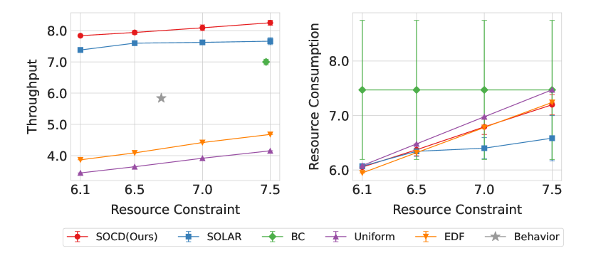
(a) Comparison of different algorithms in Real-1hop.

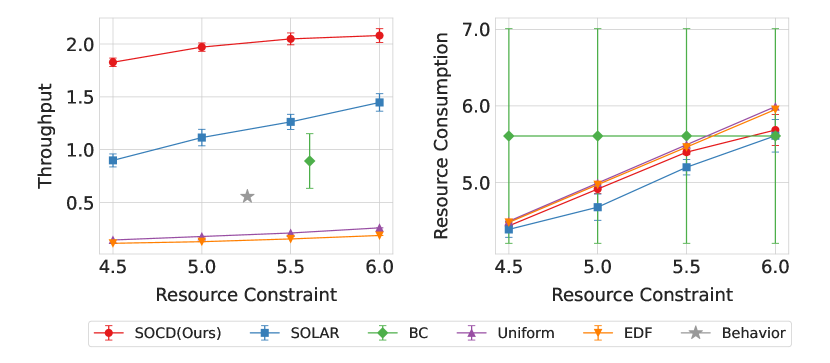
(b) Comparison of different algorithms in Real-2hop.

Figure 6: Comparison of different algorithms in two environments that utilize real-world data to model arrivals and channel conditions. Real-1hop (upper) is a single-hop environment, while Real-2hop (lower) is a 2-hop environment. The left column shows throughput, and the right column illustrates resource consumption under varying resource constraints.

The results presented in Figure 6 underscore the consistent superiority of SOCD over other algorithms, even in these more complex, real-data-driven environments. This highlights SOCD’s robustness and its ability to optimize scheduling policies despite the unpredictability and complexity inherent in real-world network data. Notably, under resource constraints of 6.1 and 6.5 in Real-1hop (Figure 6(a)) and 4.5 in Real-2hop (Figure 6(b)), the resource consumption of SOCD and SOLAR is nearly identical. However, SOCD achieves notably higher throughput than SOLAR, demonstrating its superior resource utilization efficiency in terms of algorithm performance.

5.4.4 Dynamic Changes

In this section, we further evaluate the performance of the algorithms in three more challenging environments characterized by different dynamic conditions: (1) a Real-partial scenario, where channel conditions are unavailable during decision-making, adding the challenge of partial observability; (2) a Poisson-3hop scenario, which models a 3-hop network and introduces increased complexity due to the additional hop; and (3) a Poisson-100user scenario, which simulates a high user density and requires scalable solutions to manage the increased load and complexity.

Partially Observable Systems

We begin by evaluating the algorithms in a partially observable environment Real-partial, where the channel condition is unavailable for decision-making. Despite the limited observability, SOCD not only outperforms SOLAR in equivalent conditions but also nearly matches the performance of SOLAR in fully observable settings, as evidenced by the throughput under resource constraints of 6.5 and 7.0 (Figure 6(a) and Figure 7). This highlights SOCD’s exceptional generalization capability, enabling it to perform well even when it has no knowledge of the hidden factors driving the dynamic environment.

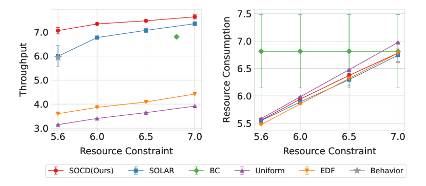
Figure 7: Comparison of different algorithms in a partially observable environment, where the channel condition is unobservable. The left plot shows throughput, and the right plot illustrates resource consumption under varying resource constraints.

More Hops

As the number of hops increases, the achievable throughput for a given amount of resource decreases, and throughput becomes dependent on a broader range of factors. This complicates the establishment of a clear correlation between resource consumption and throughput, making the scheduling task more challenging. Consequently, it becomes increasingly difficult for the policy to fully utilize the available resource under higher resource constraints. Specifically, SOLAR, which relies on a Gaussian model to approximate the policy, struggles to adapt to higher resource constraints, as evidenced by the right plot in Figure 8.

In contrast, SOCD employs a diffusion model for behavior cloning, ensuring that its performance is never worse than the behavior policy, which provides a solid foundation. Building upon this, SOCD incorporates Critic Guidance to consistently enhance its performance. As shown in Figure 8, it effectively utilizes resource to improve throughput, even as the number of hops increases.

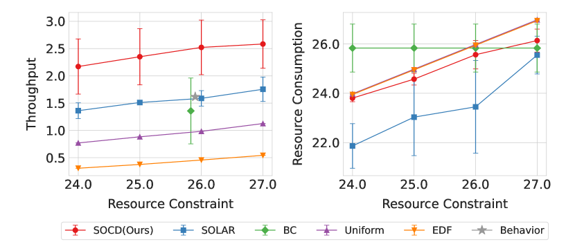
Figure 8: Comparison of different algorithms as the number of hops increases to 3. The left plot shows the throughput, while the right plot illustrates resource consumption under varying resource constraints.

Scalability in User Number

As the number of users grows to $100$, scalability becomes a significant challenge due to the rapid increase in the dimensionality of the input state and action spaces, which leads to a substantial performance degradation. To address this, SOLAR, BC, and SOCD are evaluated with their user-level decomposition versions as discussed in Section 4.1.4, which is unnecessary in four-user networks but vital in large-scale scenarios. This is because, with fewer users, the size of the state and action space is small enough for a standard network to handle, but with more users, the required network size expands to an unbearable degree, necessitating decomposition. A higher user density also introduces additional challenges, particularly in terms of stability. As the number of users grows, the variability in scheduling decisions increases, and the system becomes more prone to performance fluctuations. This leads to larger deviations in both throughput and resource consumption, making it difficult to maintain consistent performance over time.

As shown in Figure 9, traditional scheduling methods such as EDF and Uniform effectively utilize the entire resource capacity, but fail to deliver competitive throughput. Despite learning the policy in a single round without the use of Lagrange optimization, BC performs similarly to SOLAR in terms of throughput, highlighting the strong expressivity of the diffusion model. This allows BC to capture subtle variations in user index $i$ within the state space, generating more diverse scheduling strategies for each individual user. However, BC exhibits higher resource consumption and significantly larger variance, with the upper bound of its resource consumption consistently exceeding the constraint.

By incorporating Critic Guidance on top of BC, SOCD addresses these limitations and significantly outperforms both SOLAR and BC. SOCD’s throughput is consistently superior to both BC and SOLAR, and its resource variance remains well within the constraint, even at higher user densities. The superior stability in throughput and more consistent resource consumption underscore SOCD’s clear advantage.

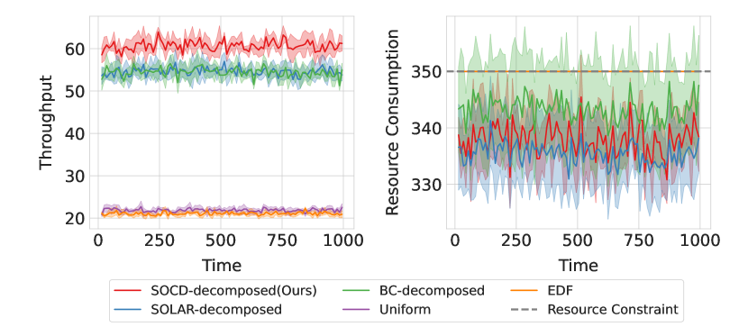
Figure 9: Comparison of various algorithms under an resource constraint of 350 as the number of users increases to 100. The left plot shows throughput, while the right plot illustrates resource consumption over time. All data are averaged across 10 time points.

In the three environments characterized by different dynamic changes discussed above, it is clear that SOLAR’s performance does not significantly exceed that of the behavior policy or the BC policy. In contrast, SOCD consistently demonstrates better generalization with more stable improvements, thanks to its diffusion-based policy component.

6 Conclusion

This paper presents Scheduling by Offline Learning with Critic Guidance and Diffusion Generation (SOCD), an offline deep reinforcement learning (DRL) algorithm designed to learn scheduling policies from offline data. SOCD introduces an innovative diffusion-based policy network, augmented by a sampling-free critic network that provides policy guidance. By integrating Lagrangian multiplier optimization into the offline reinforcement learning framework, SOCD effectively learns high-quality constraint-aware policies, eliminating the need for online system interactions during training and relying solely on offline data to autonomously refine the policies. Experiments on simulated datasets demonstrate SOCD’s robustness to diverse system dynamics and its superior performance compared to existing methods.

References

- [1] Anurag Ajay, Yilun Du, Abhi Gupta, Joshua Tenenbaum, Tommi Jaakkola, and Pulkit Agrawal. Is conditional generative modeling all you need for decision-making? arXiv preprint arXiv:2211.15657, 2022.
- [2] Abdullah Akgül, Manuel Haußmann, and Melih Kandemir. Deterministic uncertainty propagation for improved model-based offline reinforcement learning. arXiv preprint arXiv:2406.04088, 2024.
- [3] Claudio Battiloro, Paolo Di Lorenzo, Mattia Merluzzi, and Sergio Barbarossa. Lyapunov-based optimization of edge resources for energy-efficient adaptive federated learning. IEEE Transactions on Green Communications and Networking, 7(1):265–280, 2022.
- [4] Rajarshi Bhattacharyya, Archana Bura, Desik Rengarajan, Mason Rumuly, Bainan Xia, Srinivas Shakkottai, Dileep Kalathil, Ricky K. P. Mok, and Amogh Dhamdhere. Qflow: A learning approach to high qoe video streaming at the wireless edge. IEEE/ACM Transactions on Networking, 30(1):32–46, 2022.
- [5] Huayu Chen, Cheng Lu, Zhengyi Wang, Hang Su, and Jun Zhu. Score regularized policy optimization through diffusion behavior. arXiv preprint arXiv:2310.07297, 2023.
- [6] Huayu Chen, Cheng Lu, Chengyang Ying, Hang Su, and Jun Zhu. Offline reinforcement learning via high-fidelity generative behavior modeling. arXiv preprint arXiv:2209.14548, 2022.
- [7] Huayu Chen, Cheng Lu, Chengyang Ying, Hang Su, and Jun Zhu. Offline reinforcement learning via high-fidelity generative behavior modeling. ArXiv, abs/2209.14548, 2022.
- [8] Kun Chen and Longbo Huang. Timely-throughput optimal scheduling with prediction. IEEE/ACM Transactions on Networking, 26(6):2457–2470, 2018.
- [9] Minshuo Chen, Kaixuan Huang, Tuo Zhao, and Mengdi Wang. Score approximation, estimation and distribution recovery of diffusion models on low-dimensional data. arXiv preprint arXiv:2302.07194, 2023.
- [10] Tianyu Chen, Zhendong Wang, and Mingyuan Zhou. Diffusion policies creating a trust region for offline reinforcement learning. arXiv preprint arXiv:2405.19690, 2024.
- [11] Xianhao Chen and Xiao Wu. The roles of carbon capture, utilization and storage in the transition to a low-carbon energy system using a stochastic optimal scheduling approach. Journal of Cleaner Production, 366:132860, 2022.
- [12] Mingyao Cui and Linglong Dai. Channel estimation for extremely large-scale mimo: Far-field or near-field? IEEE Transactions on Communications, 70(4):2663–2677, 2022.
- [13] Miyuru Dayarathna, Yonggang Wen, and Rui Fan. Data center energy consumption modeling: A survey. IEEE Communications Surveys & Tutorials, 18(1):732–794, 2016.
- [14] Khaled MF Elsayed and Ahmed KF Khattab. Channel-aware earliest deadline due fair scheduling for wireless multimedia networks. Wireless Personal Communications, 38(2):233–252, 2006.
- [15] Kevin Frans, Danijar Hafner, Sergey Levine, and Pieter Abbeel. One step diffusion via shortcut models. arXiv preprint arXiv:2410.12557, 2024.
- [16] Scott Fujimoto and Shixiang Shane Gu. A minimalist approach to offline reinforcement learning. Advances in neural information processing systems, 34:20132–20145, 2021.
- [17] Scott Fujimoto, David Meger, and Doina Precup. Off-policy deep reinforcement learning without exploration. In International conference on machine learning, pages 2052–2062. PMLR, 2019.
- [18] Yu Han, Shi Jin, Chao-Kai Wen, and Xiaoli Ma. Channel estimation for extremely large-scale massive mimo systems. IEEE Wireless Communications Letters, 9(5):633–637, 2020.
- [19] Philippe Hansen-Estruch, Ilya Kostrikov, Michael Janner, Jakub Grudzien Kuba, and Sergey Levine. Idql: Implicit q-learning as an actor-critic method with diffusion policies. arXiv preprint arXiv:2304.10573, 2023.
- [20] Hado Hasselt. Double q-learning. Advances in neural information processing systems, 23, 2010.
- [21] Jonathan Ho, Ajay Jain, and Pieter Abbeel. Denoising diffusion probabilistic models. Advances in Neural Information Processing Systems, 33:6840–6851, 2020.
- [22] Pihe Hu, Yu Chen, Ling Pan, Zhixuan Fang, Fu Xiao, and Longbo Huang. Multi-user delay-constrained scheduling with deep recurrent reinforcement learning. IEEE/ACM Transactions on Networking, pages 1–16, 2024.
- [23] Longbo Huang, Shaoquan Zhang, Minghua Chen, and Xin Liu. When backpressure meets predictive scheduling. IEEE/ACM Transactions on Networking, 24(4):2237–2250, 2015.
- [24] Michael Janner, Yilun Du, Joshua B Tenenbaum, and Sergey Levine. Planning with diffusion for flexible behavior synthesis. arXiv preprint arXiv:2205.09991, 2022.
- [25] Chaoqiang Jin, Xuelian Bai, Chao Yang, Wangxin Mao, and Xin Xu. A review of power consumption models of servers in data centers. Applied Energy, 265:114806, 2020.
- [26] Soyi Jung, Joongheon Kim, and Jae-Hyun Kim. Joint message-passing and convex optimization framework for energy-efficient surveillance uav scheduling. Electronics, 9(9):1475, 2020.
- [27] Leila Kalankesh, Zahra Nasiry, Rebecca Fein, and Shahla Damanabi. Factors influencing user satisfaction with information systems: A systematic review. Galen Medical Journal, 9:1686, 06 2020.
- [28] Bingyi Kang, Xiao Ma, Chao Du, Tianyu Pang, and Shuicheng Yan. Efficient diffusion policies for offline reinforcement learning. Advances in Neural Information Processing Systems, 36, 2024.
- [29] Diederik Kingma and Ruiqi Gao. Understanding diffusion objectives as the elbo with simple data augmentation. Advances in Neural Information Processing Systems, 36, 2024.
- [30] Diederik Kingma, Tim Salimans, Ben Poole, and Jonathan Ho. Variational diffusion models. Advances in neural information processing systems, 34:21696–21707, 2021.
- [31] Diederik P Kingma and Max Welling. Auto-encoding variational bayes. arXiv preprint arXiv:1312.6114, 2013.
- [32] Kambiz Koosheshi and Saeed Ebadi. Optimization energy consumption with multiple mobile sinks using fuzzy logic in wireless sensor networks. Wireless Networks, 25:1215–1234, 2019.
- [33] Ilya Kostrikov, Rob Fergus, Jonathan Tompson, and Ofir Nachum. Offline reinforcement learning with fisher divergence critic regularization. In International Conference on Machine Learning, pages 5774–5783. PMLR, 2021.
- [34] Ilya Kostrikov, Ashvin Nair, and Sergey Levine. Offline reinforcement learning with implicit q-learning. arXiv preprint arXiv:2110.06169, 2021.
- [35] Aviral Kumar, Justin Fu, Matthew Soh, George Tucker, and Sergey Levine. Stabilizing off-policy q-learning via bootstrapping error reduction. Advances in Neural Information Processing Systems, 32, 2019.
- [36] Aviral Kumar, Aurick Zhou, George Tucker, and Sergey Levine. Conservative q-learning for offline reinforcement learning. Advances in Neural Information Processing Systems, 33:1179–1191, 2020.
- [37] Sascha Lange, Thomas Gabel, and Martin Riedmiller. Batch reinforcement learning. In Reinforcement learning, pages 45–73. Springer, 2012.
- [38] Henrique Lemos, Marcelo Prates, Pedro Avelar, and Luis Lamb. Graph colouring meets deep learning: Effective graph neural network models for combinatorial problems. In 2019 IEEE 31st International Conference on Tools with Artificial Intelligence (ICTAI), pages 879–885. IEEE, 2019.
- [39] Sergey Levine, Aviral Kumar, George Tucker, and Justin Fu. Offline reinforcement learning: Tutorial, review, and perspectives on open problems. arXiv preprint arXiv:2005.01643, 2020.
- [40] Jifeng Li, Xingtang He, Weidong Li, Mingze Zhang, and Jun Wu. Low-carbon optimal learning scheduling of the power system based on carbon capture system and carbon emission flow theory. Electric Power Systems Research, 218:109215, 2023.
- [41] Junling Li, Weisen Shi, Ning Zhang, and Xuemin Shen. Delay-aware vnf scheduling: A reinforcement learning approach with variable action set. IEEE Transactions on Cognitive Communications and Networking, 7(1):304–318, 2021.
- [42] Lanqing Li, Hai Zhang, Xinyu Zhang, Shatong Zhu, Junqiao Zhao, and Pheng-Ann Heng. Towards an information theoretic framework of context-based offline meta-reinforcement learning. arXiv preprint arXiv:2402.02429, 2024.
- [43] Zhuoran Li, Pihe Hu, and Longbo Huang. Offline learning-based multi-user delay-constrained scheduling. In 2024 IEEE 21st International Conference on Mobile Ad-Hoc and Smart Systems (MASS), pages 92–99. IEEE, 2024.
- [44] Qingsong Liu and Zhixuan Fang. Learning to schedule tasks with deadline and throughput constraints. In IEEE INFOCOM 2023 - IEEE Conference on Computer Communications, pages 1–10, 2023.
- [45] Yao Liu, Adith Swaminathan, Alekh Agarwal, and Emma Brunskill. Off-policy policy gradient with state distribution correction. arXiv preprint arXiv:1904.08473, 2019.
- [46] N. Loi. Predict traffic of lte network. https://www.kaggle.com/naebolo/predicttraffic-of-lte-network, 2018. Accessed: Jul. 2021.
- [47] Cheng Lu, Huayu Chen, Jianfei Chen, Hang Su, Chongxuan Li, and Jun Zhu. Contrastive energy prediction for exact energy-guided diffusion sampling in offline reinforcement learning. arXiv preprint arXiv:2304.12824, 2023.
- [48] Cheng Lu, Yuhao Zhou, Fan Bao, Jianfei Chen, Chongxuan Li, and Jun Zhu. Dpm-solver: A fast ode solver for diffusion probabilistic model sampling in around 10 steps. Advances in Neural Information Processing Systems, 35:5775–5787, 2022.
- [49] Lingling Lv, Chan Zheng, Lei Zhang, Chun Shan, Zhihong Tian, Xiaojiang Du, and Mohsen Guizani. Contract and lyapunov optimization-based load scheduling and energy management for uav charging stations. IEEE Transactions on Green Communications and Networking, 5(3):1381–1394, 2021.
- [50] Yi Ma, HAO Jianye, Xiaohan Hu, Yan Zheng, and Chenjun Xiao. Iteratively refined behavior regularization for offline reinforcement learning. In The Thirty-eighth Annual Conference on Neural Information Processing Systems, 2023.
- [51] Hongzi Mao, Ravi Netravali, and Mohammad Alizadeh. Neural adaptive video streaming with pensieve. In ACM SIGCOMM, pages 197–210, 2017.
- [52] Lluís Mas, Jordi Vilaplana, Jordi Mateo, and Francesc Solsona. A queuing theory model for fog computing. The Journal of Supercomputing, 78(8):11138–11155, 2022.
- [53] Fan Meng, Peng Chen, Lenan Wu, and Julian Cheng. Power allocation in multi-user cellular networks: Deep reinforcement learning approaches. IEEE Transactions on Wireless Communications, 19(10):6255–6267, 2020.
- [54] Ofir Nachum, Bo Dai, Ilya Kostrikov, Yinlam Chow, Lihong Li, and Dale Schuurmans. Algaedice: Policy gradient from arbitrary experience. arXiv preprint arXiv:1912.02074, 2019.
- [55] Ashvin Nair, Abhishek Gupta, Murtaza Dalal, and Sergey Levine. Awac: Accelerating online reinforcement learning with offline datasets. arXiv preprint arXiv:2006.09359, 2020.
- [56] Yasar Sinan Nasir and Dongning Guo. Multi-agent deep reinforcement learning for dynamic power allocation in wireless networks. IEEE Journal on Selected Areas in Communications, 37(10):2239–2250, 2019.
- [57] Ling Pan, Longbo Huang, Tengyu Ma, and Huazhe Xu. Plan better amid conservatism: Offline multi-agent reinforcement learning with actor rectification. In International Conference on Machine Learning, pages 17221–17237. PMLR, 2022.
- [58] Su Pan and Yuqing Chen. Energy-optimal scheduling of mobile cloud computing based on a modified lyapunov optimization method. In GLOBECOM 2017 - 2017 IEEE Global Communications Conference, pages 1–6, 2017.
- [59] Su Pan and Yuqing Chen. Energy-optimal scheduling of mobile cloud computing based on a modified lyapunov optimization method. IEEE Transactions on Green Communications and Networking, 3(1):227–235, 2018.
- [60] Seohong Park, Kevin Frans, Sergey Levine, and Aviral Kumar. Is value learning really the main bottleneck in offline rl? arXiv preprint arXiv:2406.09329, 2024.
- [61] Georgios S Paschos, Apostolos Destounis, and George Iosifidis. Online convex optimization for caching networks. IEEE/ACM Transactions on Networking, 28(2):625–638, 2020.
- [62] Xue Bin Peng, Aviral Kumar, Grace Zhang, and Sergey Levine. Advantage-weighted regression: Simple and scalable off-policy reinforcement learning. arXiv preprint arXiv:1910.00177, 2019.
- [63] Karine Pires and Gwendal Simon. Youtube live and twitch: a tour of user-generated live streaming systems. In Proceedings of the 6th ACM Multimedia Systems Conference, MMSys ’15, page 225–230, New York, NY, USA, 2015. Association for Computing Machinery.
- [64] Marcelo Prates, Pedro HC Avelar, Henrique Lemos, Luis C Lamb, and Moshe Y Vardi. Learning to solve np-complete problems: A graph neural network for decision tsp. In Proceedings of the AAAI Conference on Artificial Intelligence, volume 33, pages 4731–4738, 2019.
- [65] Yiming Qin, Huangjie Zheng, Jiangchao Yao, Mingyuan Zhou, and Ya Zhang. Class-balancing diffusion models. 2023 IEEE/CVF Conference on Computer Vision and Pattern Recognition (CVPR), pages 18434–18443, 2023.
- [66] Ali Rahimi and Benjamin Recht. Random features for large-scale kernel machines. Advances in neural information processing systems, 20, 2007.
- [67] P. Ramachandran, B. Zoph, and Q. V. Le. Swish: A self-gated activation function. arXiv preprint arXiv:1710.05941, 2017.
- [68] Aditya Ramesh, Prafulla Dhariwal, Alex Nichol, Casey Chu, and Mark Chen. Hierarchical text-conditional image generation with clip latents. arXiv preprint arXiv:2204.06125, 2022.
- [69] Shideh Rezaeifar, Robert Dadashi, Nino Vieillard, Léonard Hussenot, Olivier Bachem, Olivier Pietquin, and Matthieu Geist. Offline reinforcement learning as anti-exploration. In Proceedings of the AAAI Conference on Artificial Intelligence, volume 36, pages 8106–8114, 2022.
- [70] Ziv Scully, Mor Harchol-Balter, and Alan Scheller-Wolf. Simple near-optimal scheduling for the m/g/1. ACM SIGMETRICS Performance Evaluation Review, 47(2):24–26, 2019.
- [71] Noah Y Siegel, Jost Tobias Springenberg, Felix Berkenkamp, Abbas Abdolmaleki, Michael Neunert, Thomas Lampe, Roland Hafner, Nicolas Heess, and Martin Riedmiller. Keep doing what worked: Behavioral modelling priors for offline reinforcement learning. arXiv preprint arXiv:2002.08396, 2020.
- [72] Rahul Singh and P. R. Kumar. Throughput optimal decentralized scheduling of multihop networks with end-to-end deadline constraints: Unreliable links. IEEE Transactions on Automatic Control, 64(1):127–142, 2019.
- [73] Jascha Sohl-Dickstein, Eric Weiss, Niru Maheswaranathan, and Surya Ganguli. Deep unsupervised learning using nonequilibrium thermodynamics. In International Conference on Machine Learning, pages 2256–2265. PMLR, 2015.
- [74] Jiaming Song, Chenlin Meng, and Stefano Ermon. Denoising diffusion implicit models. arXiv preprint arXiv:2010.02502, 2020.
- [75] Yang Song and Stefano Ermon. Generative modeling by estimating gradients of the data distribution. Advances in Neural Information Processing Systems, 32, 2019.
- [76] Yang Song, Jascha Sohl-Dickstein, Diederik P Kingma, Abhishek Kumar, Stefano Ermon, and Ben Poole. Score-based generative modeling through stochastic differential equations. arXiv preprint arXiv:2011.13456, 2020.
- [77] Adith Swaminathan and Thorsten Joachims. Batch learning from logged bandit feedback through counterfactual risk minimization. The Journal of Machine Learning Research, 16(1):1731–1755, 2015.
- [78] Haoyue Tang, Jintao Wang, Linqi Song, and Jian Song. Minimizing age of information with power constraints: Multi-user opportunistic scheduling in multi-state time-varying channels. IEEE Journal on Selected Areas in Communications, 38(5):854–868, 2020.
- [79] W. Taotao, X. Jiantao, X. Wensen, C. Yucheng, and Z. Shengli. Wireless signal strength on 2.4 ghz (wss24) dataset. https://github.com/postman511/Wireless-Signal-Strength-on-2.4GHz-WSS24-dataset, 2021. Accessed: Feb. 17, 2022.
- [80] Natalia Vesselinova, Rebecca Steinert, Daniel F Perez-Ramirez, and Magnus Boman. Learning combinatorial optimization on graphs: A survey with applications to networking. IEEE Access, 8:120388–120416, 2020.
- [81] Jialin Wan, Sen Lin, Zhaofeng Zhang, Junshan Zhang, and Tao Zhang. Scheduling real-time wireless traffic: A network-aided offline reinforcement learning approach. IEEE Internet of Things Journal, 2023.
- [82] Xiaohan Wang, Lin Zhang, Yongkui Liu, and Chun Zhao. Logistics-involved task scheduling in cloud manufacturing with offline deep reinforcement learning. Journal of Industrial Information Integration, 34:100471, 2023.
- [83] Zhendong Wang, Jonathan J Hunt, and Mingyuan Zhou. Diffusion policies as an expressive policy class for offline reinforcement learning. arXiv preprint arXiv:2208.06193, 2022.
- [84] Zhengyi Wang, Cheng Lu, Yikai Wang, Fan Bao, Chongxuan Li, Hang Su, and Jun Zhu. Prolificdreamer: High-fidelity and diverse text-to-3d generation with variational score distillation. Advances in Neural Information Processing Systems, 36, 2024.
- [85] Yifan Wu, George Tucker, and Ofir Nachum. Behavior regularized offline reinforcement learning. arXiv preprint arXiv:1911.11361, 2019.
- [86] Zhen Xiao, Lei Guo, and John Tracey. Understanding instant messaging traffic characteristics. In 27th International Conference on Distributed Computing Systems (ICDCS ’07), pages 51–51, 2007.
- [87] Kun Yang, Chengshuai Shi, Cong Shen, Jing Yang, Shu-ping Yeh, and Jaroslaw J Sydir. Offline reinforcement learning for wireless network optimization with mixture datasets. IEEE Transactions on Wireless Communications, 2024.
- [88] Han Zhang, Wenzhong Li, Shaohua Gao, Xiaoliang Wang, and Baoliu Ye. Reles: A neural adaptive multipath scheduler based on deep reinforcement learning. In IEEE INFOCOM 2019 - IEEE Conference on Computer Communications, pages 1648–1656, 2019.