A Denser Hydrogen Inferred from First-Principles Simulations Challenges Jupiter’s Interior Models

Abstract

First-principle modeling of dense hydrogen is crucial in materials and planetary sciences. Despite its apparent simplicity, predicting the ionic and electronic structure of hydrogen is a formidable challenge, and it is connected with the insulator-to-metal transition, a century-old problem in condensed matter. Accurate simulations of liquid hydrogen are also essential for modeling gas giant planets. Here we perform an exhaustive study of the equation of state of hydrogen using Density Functional Theory and quantum Monte Carlo simulations. We find that the pressure predicted by Density Functional Theory may vary qualitatively when using different functionals. The predictive power of first-principle simulations is restored by validating each functional against higher-level wavefunction theories, represented by computationally intensive variational and diffusion Monte Carlo calculations. Our simulations provide evidence that hydrogen is denser at planetary conditions, compared to currently used equations of state. For Jupiter, this implies a lower bulk metallicity (i.e., a smaller mass of heavy elements). Our results further amplify the inconsistency between Jupiter’s atmospheric metallicity measured by the Galileo probe and the envelope metallicity inferred from interior models.

I Introduction

Compressed hydrogen (H) has been subject of both theoretical and experimental research for nearly a century[1, 2]. Most experimental studies have focused on exploring the complex phase diagram of hydrogen, particularly the insulator-to-metal transition, which has been referred to as the holy grail of condensed matter physics[3, 4, 5, 6, 7]. This phase transition, when occurring in the liquid sector[8, 9, 10] of the pressure-temperature ($P$-$T$) diagram, has significant implications for planetary science, as it affects the inferred planetary internal structure and determines the conditions for magnetic field generation in gas giant planets [11]. Since the gas giants in the Solar System are predominantly composed of hydrogen, qualitative discoveries and quantitative assessments of the thermodynamics of this simple element are crucial to constraining the compositions and internal structures of these planets[e.g., 2]. Constraining the equation of state (EoS) of hydrogen has become even more important recently as the Juno and Cassini missions provided accurate measurements of the gravitational fields of Jupiter and Saturn [12, 13]. The gravitational fields are used to constrain the planetary density profiles[14]. Given the small uncertainties in the gravity field measurements, minor differences in the hydrogen EoS can result in relatively large differences in the inferred internal structure [15, 16]. Recent developments have opened new questions in planetary science and have affected the way we view giant planets. Interestingly, Jupiter interior models have found that the planet is inhomogeneous in composition [17]. In addition, interior models suggest that Jupiter’s deep interior is rather metal-poor [18, 19, 17, 20, 16] while atmospheric measurements from the Galileo probe indicate that Jupiter’s atmosphere is enriched by a factor of $\sim 3$ compared to solar composition. This discrepancy could have several explanations, one of which is that the behavior of hydrogen is not yet understood to within 1% accuracy [21]. Given the precision of the gravity measurements, it is crucial to ensure that theoretical uncertainties are compatible with these measurements. As a result, obtaining an accurate H-EoS is of great importance.

Since the experimental data at planetary conditions are not accurate enough, numerical models must be used. The range of pressure and temperature encountered from the planetary surface to the center varies by several orders of magnitude, and therefore different theories are used. The choice of method or theory for calculating the EoS depends on the temperature and density conditions. From ambient to $\approx$ 0.1 g/cc density, hydrogen is present in a weakly interacting molecular form, and the Saumon Chabrier van Horn (SCvH) EoS [22] is utilized. Hydrogen becomes a challenging system at higher density, where pressure-induced dissociation occurs, hence, one needs to treat the system as a genuine many-electron quantum mechanical problem. In this case, first-principle (or ab initio) molecular dynamics (MD) simulations are used.

Most methods provide an EoS that relates the pressure $P$ and density $\rho$ with temperature $T$. For instance, MD simulations fix $\rho$ and $T$ and output the corresponding $P$. While this information could be sufficient to explore phase diagrams, planetary models, which are often adiabatic, also require knowledge of the entropy, $S$. This information is computed through post-processing of the MD data. However, previous studies that used different methods have led to rather different inferred entropy, even when considering compatible $P$ vs $\rho$ input data[23, 24, 15]. These differences significantly affected the predicted internal structure of Jupiter where the inferred masses of heavy elements could differ by a factor of $\sim$5. [15, 25] Recently, in Ref [26], we addressed this aspect conclusively, showing that the source of entropy error stems from thermodynamic inconsistencies at the boundaries, where different theories are joined to produce a single EoS. By solving this major methodological issue, we can now address the final fundamental weaknesses of the various hydrogen EOSs, namely, the choice of the electronic structure theory.

There have been several widely used ab-initio hydrogen EoSs for planetary modeling, namely the Chabrier, Mazevet and Soubiran (CMS19)[27], Militzer and Hubbard (MH13)[24], and the Rostock EoS (REOS2[23], REOS3[28]). All these EOSs have a common origin, as their ab initio part is based on density functional theory (DFT), with the specific choice of the Perdew-Burke-Ernzerhof (PBE) functional as the exchange-correlation (xc) functional.

While in principle DFT is an exact theory (if the exact xc functionals were known), in practice, the choice of an approximation for the xc functionals introduces some errors[29]. Although the PBE functional is the most widely used in materials science, due to an excellent balance between providing reasonable results and computational cost, there is no guarantee that it is suitable for a system as peculiar as dense hydrogen. In fact, it is known that the choice of functional has a significant impact on predicting the phase diagram at low temperatures, such that resorting to higher levels of theory is considered fundamental.[30, 10, 31, 32]

In this work, we explore the effect of the functionals on the H-EoS and show that other reasonable xc functionals yield pressure outputs that may differ by $\pm 20\%$, at planetary conditions, compared to PBE, i.e., compared to the most-commonly used EoS tables in planetary science. This is far exceeding the level of accuracy required for planetary modeling. In the absence of an experimental benchmark, valid over the whole range of $P$ and $T$ of interest, the only possible way forward to identify the most accurate xc functional is through a comparison with a higher level of theory, quantum Monte Carlo (QMC).

This manuscript is organized as follow. In Sect. II we outline the first-principle methods to compute EoS, In Sect. III we compare several DFT functionals and identify the best performing one using QMC calculations. In Sect. IV we use this information to compute a thermodynamically consistent EoS, including entropy, which is then used in the interior models of Sect. V. We discuss the implications for Jupiter modeling in Sect. VI.

II Ab-initio electronic structure methods

The majority of hydrogen in gas giant planets exists in a density regime where a fully quantum treatment of the electrons is essential[1, 33]. The interacting $N$-electron problem is the central theme in materials science and quantum chemistry, and it inevitably requires approximations to be solved [34]. The key concept with which we want to begin is that being ab initio, or first-principle, does not mean that a method is exact; rather that it does not require ad hoc fits to experimental data. In this Section, we outline the theoretical foundations and the various approximations that must be made to address the electronic structure problem. The starting point is the (non-relativistic) Hamiltonian of $N$ electrons and $N$ protons in the so-called first quantization formalism:

$$\hat{H} =\hat{H}_{e}+\hat{H}_{p}+\hat{H}_{p},$$ (1)

$$\hat{H}_{e} =-\frac{\hbar^{2}}{2m_{e}}\sum_{i=1}^{N_{e}}\nabla_{i}^{2}+\frac{1}{2}\sum_{i\neq j}^{N_{e}}{\frac{e^{2}}{|\textbf{r}_{i}-\textbf{r}_{j}|}}\,,$$ (2)

$$\hat{H}_{p} =-\frac{\hbar^{2}}{2m_{p}}\sum_{i=1}^{N_{p}}\nabla_{i}^{2}+\frac{1}{2}\sum_{i\neq j}^{N_{p}}{\frac{e^{2}}{|\textbf{R}_{i}-\textbf{R}_{j}|}}\,,$$ (3)

$$\hat{H}_{ep} =-\sum_{i,j=1}^{N}{\frac{e^{2}}{|\textbf{r}_{i}-\textbf{R}_{j}|}}\,,$$ (4)

where $\textbf{r}=\{\textbf{r}_{1},\dots\textbf{r}_{N}\}$ and ${\bf x}=\{{\bf R}_{1},{\bf R}_{2},\cdots,{\bf R}_{N}\}$, are the electrons and protons coordinates, respectively. The problem simplifies if we consider only the electrons as quantum particles, and the protons as classical objects. Then, following the ground-state Born-Oppenheimer (BO) approximation, the electrons are considered to be in their instantaneous ground state, while the classical nuclei ${\bf x}$ move accordingly to the potential energy surface $E_{e}[{\bf x}]$ corresponding to this ground state. Notice that the BO holds also in case of a quantum description of the nuclei. In this case, one could adopt path-integral formalism to describe the quantum delocalization of the protons at low temperatures.[35, 36] In this work, we employ the classical nuclei approximation, as it is exact at temperatures relevant to planetary science, i.e., above 2000 K.[36] While our EoS extends to lower temperatures, where nuclear quantum effects may not be negligible[37] (e.g., at 500 K), we do this to maintain consistency with other EoS tables and to analyze the temperature dependence of the variation between different xc functional predictions, which can be of independent interest for the high-pressure community.

Even within the Born-Oppenheimer approximation, solving the fixed-nuclei Schrödinger equation,

$$(\hat{H}_{e}+\hat{H}_{ep}[{\bf x}])\leavevmode\nobreak\ \psi({\bf r})=E_{e}[{\bf x}]\leavevmode\nobreak\ \psi({\bf r}),$$ (5)

where $\psi({\bf r})$ is a $N$-electron non-separable wavefunction, obeying the fermionic anti-symmetry principle, requires computational resources that grow exponentially with $N$[38].

Previous works have shown that one needs to reach a system of about a hundred hydrogen atoms, with appropriate schemes to mitigate electronic finite-size effects, to attain a converged EoS[39]. Therefore, simulating a system of this size exactly can only be achieved using approximations. Several methods exist, with the key difference being that some methods features uncontrolled approximations, while others can be systematically improved.

II.1 Density Functional Theory

Density Functional Theory is the most commonly used ab initio simulation method for electronic systems with $N>100$ electrons.[29, 40] Its widespread use relies on a relatively simple theoretical framework and the development of several software packages that allow fast and reproducible calculations [41, 42]. The fundamental idea behind DFT is that it is possible to describe the ground-state properties of an $N-$ electron system in terms of the three-dimensional electronic density $\rho_{e}$ alone, without any explicit reference to the $3N$-dimensional many-body wave function.[43, 44] Therefore, one could search for the solution of Eq. (5) in the space of antisimmetrized products of single particle orbitals $\phi({\bf r}_{j})$, a much simpler task. Indeed, even if the exact solution of Eq. (5) is a non-separable wavefunction, the wavefunction constructed from the orbitals $\phi({\bf r}_{j})$ could yield the same exact electronic density. To obtain the single-particle orbitals it is sufficient to work with a one-body Hamiltonian of the form:

$$\hat{H}_{\textrm{DFT}}[{\bf x}]=-\frac{\hbar^{2}}{2m_{e}}\sum_{i=1}^{N}\nabla_{i}^{2}+\hat{H}_{ep}[{\bf x}]+\hat{V}_{\mathrm{xc}}[\rho_{e}].$$ (6)

Notice the replacement of the explicit two-body electron-electron Coulomb term in Eq. (2) with a potential $V_{\mathrm{xc}}$ which should only depends on the electron density. This approach would be exact if the functional form key term in Eq. (6), the exchange-correlation functional $V_{\mathrm{xc}}$ is known. Unfortunately, this term can only be approximated, such that the DFT solution for the electronic density, and the other properties, is not exact. For more details, we refer to comprehensive reviews of the DFT method[45, 40].

There are various theories, each offering different prescriptions for constructing $V_{\mathrm{xc}}$. Each of these is labeled by the name of the xc functional . PBE functional[46], introduced 30 years ago, is the most used in materials science, and the only one used so far to create EoS tables for hydrogen[28, 27] and hydrogen-helium[24, 47] More recent functionals include the BLYP functional[48, 49], which is most commonly used in chemical problems, functionals with van-der-Waals corrections like vdW-DF[50, 51] and vdW-DF2,[52] and the recently released strongly constrained and appropriately normed (SCAN) functional[53]. These functionals have been applied to pure-hydrogen (and hydrogen-helium mixtures)[54, 36, 55, 56, 57, 58, 59], but never to compute the H-EoS.

It is crucial to note that (1) the sophistication level or release date of a functional does not necessarily mean it is better than its predecessors, and (2) in general, the accuracy of a functional is system-dependent[29] For most materials science problems, precise experimental data is available, so one can a posteriori select which xc functional performs best for a given problem. This is not the case for hydrogen at order of 100 GPa pressures, where experiments can only provide incomplete -and sometimes contested- results, such as phase boundaries.[6, 9, 10, 60, 61, 62]

Unfortunately, the choice of the xc functional has a qualitative impact on the phase diagram of hydrogen and quantitatively alters its EoS. The predicted phase boundaries between insulating solid phases[30], as well as the insulator-to-metal transition[63, 10, 64], can vary by up to 100$\%$ depending on the functional chosen. Given this body of evidence, there is no rigorous justification for using a PBE-based EoS because (1) PBE is not expected to be the best-performing functional for this system, since it overestimates the molecular bond lenght by $\sim 5\%$, and overstabilizes the metallic phase[63, 54, 65], and (2) numerical predictions obtained with PBE do not align with experimental results in the solid region[30].

Details of our DFT setup are provided in Appendix A.

II.2 Quantum Monte Carlo

While DFT is an incredibly successful technique, it faces challenges describing strong electronic correlations[66, 67, 68] and non-covalent interactions[69, 70], due to the approximate functional form to describe the xc effects between the electrons. For this reason, and especially in high-pressure physics, where experiments do not represent a quantitative benchmark, DFT results should be validated against higher-level theories.

Quantum Monte Carlo is among one of these methods as it represents the most reliable choice available for medium-sized system (e.g. order of 100-200 electrons) [71, 69]. The main advantages of QMC are: (1) QMC relies on a many-body theory with a natural and explicit description of electron correlations, and its accuracy is systematically improvable. (2) QMC gives accurate results exhibiting, at the same time, a comparable scaling of computational cost with system size with DFT (although usually with a much larger prefactor). (3) New supercomputer architectures are becoming more and more suitable for intrinsically parallel techniques such as Monte Carlo rather than for DFT or quantum chemistry methods.[72] Therefore, the system sizes that can be simulated by QMC are substantially larger compared to the ones of Couple Cluster (CC) theory, which is considered the gold standard (in its CCSD(T) formulation[73, 74]) for quantum chemistry calculations. This enables the possibility of performing electronic structure simulations on bulk systems comparable with DFT, and to benchmark xc functionals.

In this work we employ two QMC techiques: Variational Monte Carlo (VMC) and Lattice Regularized Diffusion Monte Carlo (LRDMC) [75] implemented in the TurboRVB package [72, 76]. The first is a purely variational method, while the second is a projection method. The central object of VMC is the trial-wave function $\psi_{\boldsymbol{\theta}}({\bf r})$ which depends explicitly on the $3N$-dimensional vector of electron positions, ${\bf r}$ (notice that for hydrogen the number of electrons is the same as the number of protons), and parametrically on a set of optimizable parameters $\boldsymbol{\theta}$. The wavefunction also implicitly depends on the ionic coordinates, ${\bf x}$, as it is constructed using an atom-centered basis set. Appendix B presents further details on the functional form of the trial state $\psi_{\boldsymbol{\theta}}({\bf r})$.

The parameters $\boldsymbol{\theta}$ are optimized in order to minimize the energy:

$$E_{\boldsymbol{\theta}}[{\bf x}]=\frac{\langle\psi_{\boldsymbol{\theta}}({\bf r;{\bf x}})|H|\psi_{\boldsymbol{\theta}}({\bf r};{\bf x})\rangle}{\langle\psi_{\boldsymbol{\theta}}({\bf r;{\bf x}})|\psi_{\boldsymbol{\theta}}({\bf r};{\bf x})\rangle}\geq E_{0}[{\bf x}]\leavevmode\nobreak\ ,$$ (7)

where the expectation value needs to be evaluated as $3N$-dimensional integral over the coordinate ${\bf r}$, and $E_{0}$ is the exact ground state energy. This high-dimensional integral cannot be computed using quadrature methods but instead with the Monte Carlo method, hence the name of the technique.

The main difference with the DFT framework is that QMC features the exact Hamiltonian (Eq. 5) while the approximations are transferred to the wavefunction. Crucially, the trial wave function can be systematically improved both in its functional form and in the number of parameters. For example, one could enhance the description of 2-, 3-, or 4-body electron-ion correlations, or expand the basis set used to define the wave function (see Appendix  B). This mirrors the popular machine learning methods, where accuracy increases with the complexity of the network or model.

Following this parallel with ML,[77, 78, 79, 80] VMC also needs efficient and stable methods to optimize the parameters in order to be practical. In our case, the wave function features 13315 tunable parameters (only in the Jastrow factor), which are optimized using the Stochastic Reconfiguration method of Refs. [81, 82]. The optimized trial wave function obtained from a VMC calculation serves as the starting point for the LRDMC method.

The LRDMC method provides even more accurate results and offers another way to systematically improve the many-body wave function, and has been employed successfully in Refs. [83, 84]. The computational settings employed in the calculations are provided in Appendix  B. Further details of the LRDMC method can be found in Ref. 75, 85, 72.

Concerning the computational cost, VMC and LRDMC electronic structure calculations are more expensive than DFT calculations by more than an order of magnitude. Moreover, LRDMC with the lattice discretization parameter of 0.3 bohr is 3 times more expensive than VMC, and therefore has been used mostly to validate the accuracy of VMC, over the full range of density and pressure. Additionally, direct LRDMC simulations will be used in the range of 0.2–0.5 g/cc and 2000–5000 K for the xc functional benchmarking. This is because the VMC pressure estimate is affected by an error of about 1 GPa compared to LRDMC. While this value is negligible at moderate to high pressure, it cannot be neglected at low pressures. For this reason, we switch to LRDMC in this region of the phase diagram.

In summary, we computed energies and pressures of 4512 and 832 structures by VMC and LRDMC, respectively. These atomic structures are sampled using PBE-driven molecular dynamics (see procedure outlined in Sect. III.2). Notice that, since the pressures were computed numerically by fitting the potential energy surfaces computed with 7 volumes for each structure as described in Appendices  C and D, we actually computed seven times larger numbers of structures (i.e., 31584 and 5824 structures by VMC and LRDMC calculations, respectively). These calculations were carried out on the Fugaku supercomputer with total CPU costs of approximately 57 million and 25 million CPU hours for the VMC and LRDMC parts, respectively. It is clear that brute-force MD simulations using QMC (while technically possible[86, 87, 31]) would be impractical in the full $\rho$-T range, as they would require hundreds of times more computational resources (note that each DFT-MD simulation at a fixed density and temperature involves around 10,000 electronic structure calculations).

A possible strategy could be to use the QMC dataset as a training set for a machine learning potential[88, 89, 90, 91]. However, there are outstanding technical challenges[92] and we hope to address this in future studies.

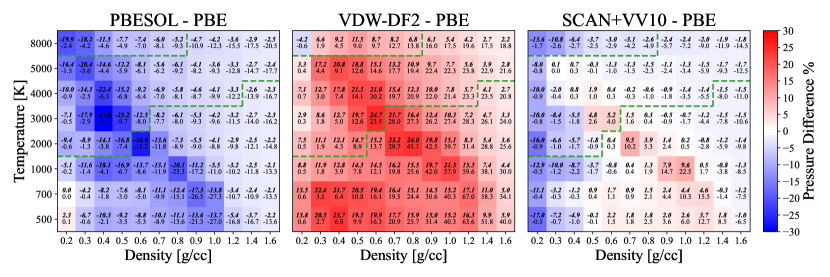
Figure 1: Equation of state of hydrogen using selected DFT approximations. We plot the difference between the EoS calculated with three different xc DFT potentials, PBEsol (left), vdW-DF2 (middle), and SCAN+vv10 (right) versus the REOS3 data (which is obtained with the PBE functional). In each cell we report the relative (above, in $\%$) and the absolute (below, in GPa) differences. The color code refers to the relative values. The green dashed lines highlight the ‘planetary’ region of temperatures and densities which is of particular interest for interior models (see Sect. III.2).

II.3 Molecular dynamics

In the previous sections, we introduced two different computational methods to solve the many-body electronic problem at fixed ionic configurations. The output of these methods includes not only the potential energy surface, $E_{e}[{\bf x}]$, but also the electronic forces and the electronic contribution to the pressure, which is the dominant factor at the densities considered here.

To obtain the EoS, we need to average over the ionic positions. This task is obtained using molecular dynamics, where the motion of $N$ interacting ions is numerically integrated based on the forces acting between them.[35] By employing an appropriate thermostat, the canonical ensemble can be simulated, at a constant temperature $T$.[93] For sufficiently large systems and long simulation times, thermodynamic properties such as internal energy, stress, and pressure can be determined by averaging their values over the trajectory, and statistical methods can be used to calculate reliable error bars. The forces between ions are computed at each step of the dynamics from the computed electronic structure. It is important to note that different levels of theory (or exchange-correlation functionals) produce different forces, which in turn affect the equilibrium distribution generated.

After an equilibration period, the MD sequentially generates configurations ${\bf x}_{i}$ distributed according to the Boltzmann weights $p({\bf x}_{i})\propto e^{-\beta E({\bf x}_{i})}$ ($\beta=1/T$, in atomic units). We can calculate the energy $E({\bf x}_{i})$, the ionic forces ${\bf F}({\bf x}_{i})$, and the pressure $P({\bf x}_{i})$ for each configuration ${\bf x}_{i}$. Indeed, all the quantities above are understood having also a subscript $\{A,B,C,\cdots\}$ indicating the level of theory we are using to calculate them. At each thermodynamic point $(\rho,T)$ we will obtain different average values of energy $\langle E\rangle_{A}$, $\langle E\rangle_{B}$ etc., and pressure $\langle P\rangle_{A}$, $\langle P\rangle_{B}$ etc., not only because the output $E_{A}({\bf x}_{i})$ and $P_{A}({\bf x}_{i})$ is different from $E_{B}({\bf x}_{i})$ and $P_{B}({\bf x}_{i})$ at the same ionic configuration ${\bf x}_{i}$, but also because the generated configurations will also be different.

To summarize, we will run different MD using several xc-correlation functionals, and compute different EoS which correspond to these different electronic structure theories. Moreover, we will use a dataset of uncorrelated configurations $\{\bar{\bf x}\}_{\textrm{PBE}}^{(\rho,T)}$, for each $(\rho,T)$ point, obtained at the DFT-PBE level of theory and will recompute the energies and pressure using our QMC method as well as 15 other different DFT xc functionals. This will allows us to select the best performing xc functional against QMC data.

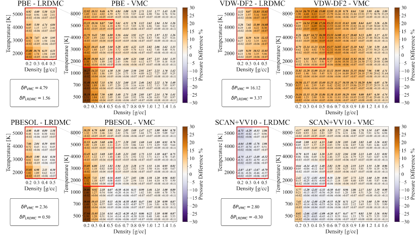
Figure 2: Benchmarks of selected DFT xc functionals against VMC and LRDMC pressure data. We plot the pressure error as defined in Eq. 8 of PBE, PBEsol, vdW-DF2, and SCAN+vv10 compared to VMC (full table) and LRDMC (left insets) benchmarks. In each cell we report the relative (above, in $\%$) and the absolute (below, in GPa, with associated statistical error) differences. The color code refers to the relative values. Lighter colors indicate smaller errors. The values in the box are the error averaged only over the ‘planetary’ region, LRDMC where it is present and VMC otherwise. This is the same region highlighted by the green dashed lines in Fig. 1.

III Selecting the most accurate equation of state

III.1 Direct DFT-MD simulations with various xc functionals

We perform direct MD simulations using four DFT theories: PBE, PBEsol[94], vdW-DF2, and SCAN-VV10[95], across a density range of 0.2–1.6 g/cc and a temperature range of 500–8000 K. We use a 12-point density grid and an 8-point temperature grid, resulting in 96 ($\rho$, T) thermodynamic points. The first set of simulations, using PBE, is primarily used to validate our setup against REOS3, which also employs the same xc functional (in this range) but a different DFT code and particle number. We find that our PBE EoS is perfectly consistent with the REOS3 pressure output.

We then run the 96 MD simulations for each of the other three functionals and compare the new EoS against REOS3 in Fig. 1. We observe that the changes in the EoS are significant. The PBEsol functional, a modified version of PBE designed to improve the description of solids[94], and that could be better for high-pressure materials[96], predicts a denser liquid across the entire range, with peaks of up to 20-30$\%$ denser liquid at 3000-4000 K and 0.4 g/cc (i.e., along Jupiter’s adiabatic curve). For clarity, PBEsol yields a lower pressure than REOS at fixed density, therefore by inverting the $P-\rho$ relation, it predicts a denser liquid at fixed pressure. In contrast, the vdW-DF2 functional predicts a much lighter fluid across the table. In this case, we find a 20$\%$ lighter fluid at 4000 K and 0.5–0.6 g/cc. Finally, the SCAN-VV10 functional shows smaller variations compared to REOS3, predicting either a denser or lighter liquid in different regions of the phase diagram.

It is noticeable that the largest deviations from REOS3 occur along a diagonal line in the center of the plot. This is due to the different positions of the metal-to-insulator transition predicted by the various functionals. For example, PBE (which is the basis of REOS3) underestimates the transition pressure compared to vdW-DF2[10]. Between the two predicted phase boundaries, PBE stabilizes an atomic liquid, while vdW-DF2 predicts a molecular one, leading to much differing EoS.

It is also interesting to observe the pressure changes in a subset of ($\rho$, T) values relevant to gas giants. While PBEsol (vdW-DF2) consistently predicts a denser (lighter) fluid, the SCAN-VV10 functional shows a slightly denser fluid across most of the range, except for the density interval between 0.3 and 0.6 g/cc, at about 4000 K, where it predicts a lighter material.

Note that all four functionals considered so far, PBE, PBEsol, vdW-DF2, and SCAN+vv10 are plausible choices. Indeed, PBE has been the most widely used for describing the solid and liquid phase diagrams in the 00’s and the early 10’s of this century[97, 98, 99, 39, 100]. Later, van der Waals corrected functionals, such as the vdW-DF2, has been introduced among the employed for studying this and related systems[63, 10, 57, 56]. Finally, the newly introduced family of SCAN functionals, has also been used for hydrogen yielding a liquid-liquid phase boundary which seems to be more in agreement with QMC predictions compared to other functionals.[59, 101] In this regard, while previous DFT and QMC works have focused on determining the liquid-liquid phase boundary, the calculation of a complete EoS table using functionals different that PBE is a new contribution of the manuscript. For example, it is known that SCAN improves the description of electronic gaps over PBE. However, this fact may simply improve the prediction for the metallization transition with no guarantees in improving uniformly also the EoS.

III.2 Benchmarking results

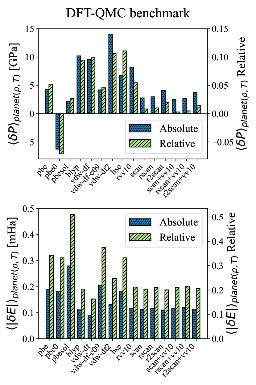
Figure 3: Pressure and energy benchmarks. Results for the benchmark of Pressure and Energy per atom from all the set of DFTxc against QMC results computed as shown in Eq.10. The set of $(T,\rho)$ over which the benchmark has been computed is the one highlighted in Fig.1 by the green dashed line, with LRDMC results where they are present and VMC elsewhere.

It is not possible to choose a functional in the absence of reliable experimental results or comprehensive data from higher-level theories such as QMC. In 2014, Clay and collaborators benchmarked pressure, energy, and bond lengths of selected solid structures, as well as representative liquid structures, of several xc functionals against QMC data [54]. The liquid structures used in Clay et al.’s work were sampled at T = 1000 K and under three density regimes, corresponding to molecular, atomic, and mixed fluids. The main difference compared to our work is that (1) we feature a much larger dataset in liquid phase, utilizing 47 uncorrelated 128-atoms structures for each of the 96 thermodynamic conditions in our EoS table. This provides a better understanding of DFT errors across the entire range, especially for planetary science applications. (2) We test more functionals including those not developed at that time, and this is crucial given that SCAN is the best performing one. (3) Additionally, another significant difference is in the QMC setup. Clay et al.[54] employed a different functional form for the trial wavefunction in VMC, a different projective QMC approach, and a smaller system size of 54 protons compared to our current study. Therefore, we expect quantitative differences that may affect the results.

Their main finding of Ref. [54] was that, at least for the set of functionals considered at the time, no clear ‘winner’ could be identified, as the performance of most DFT functionals depended on the property being studied and the thermodynamic conditions (e.g., metallic or insulating). Moreover, they concluded that PBE did not perform well for the energetics and properties of molecular bonds.

Finally, other groups have employed QMC at the fixed-node DMC level, focusing on solid structures.[102] This information have also been used to assess the predictive power of various xc functionals. For instance, that dataset suggested that vdW-DF2 perform better than vdW-DF [57].

In this work, for consistency, we do not use previous QMC data but we construct from scratch our validation dataset, following the procedure of Ref. [54], but using a much finer mesh of density and temperatures. For each of the 96 $\rho$ and $T$ combinations, we extract $M=47$ uncorrelated structures ${\bf x}_{i}$ from the PBE molecular dynamics and calculate the VMC energy and pressures. At lower densities, from 0.2 to 0.5 g/cc, and temperatures between 2000 and 5000 K (i.e. for a total of 16 thermodynamic points) we also calculate the LRDMC outputs. This is needed because at low densities the pressure difference between DFT data and VMC falls within the estimated accuracy of VMC, so a more accurate QMC method is needed. The total number of structured considered is 4512. We choose not to utilize the VMC forces as benchmark as they can be affected by a residual error [103, 104, 92], as explained in Appendix C. This error may not be negligible if our task is to provide a quantitative benchmark of DFT, given that we also expect several xc functional being competitive with each other.

We benchmark 15 functionals, belonging to the set $\mathrm{DFTxc}=\{$ PBE, PBEsol, PBE0[105], BLYP, vdW-DF, vdW-DF2, vdw-DF2-c09[106], rVV10[107, 108], HSE[109], SCAN, rSCAN[110], r2SCAN[111], SCAN+vv10, rSCAN+vv10, r2SCAN+vv10 $\}$. For each ($\rho,T$) condition, we introduce the following metrics. The pressure error of a given functional against QMC is defined as

$$\delta P^{(\rho,T)}=\frac{1}{M}\sum_{{\bf x}_{i}\in\mathcal{S}^{(\rho,T)}}\left(P^{\mathrm{DFTxc}}({\bf x}_{i})-P^{\mathrm{QMC}}({\bf x}_{i})\right)$$ (8)

where $\mathcal{S}^{(\rho,T)}$ is the set of $M$ uncorrelated and physically representative of the thermodynamic conditions ($\rho,T$). Concering $P^{\mathrm{QMC}}$ will use both pressures calculated with VMC, $P^{\mathrm{VMC}}$ and LRDMC, $P^{\mathrm{LRDMC}}$, when available.

Assessing the energy error is more cumbersome given that energies are defined up to a offset. We adopt a strategy similar to Ref. [54], and define the energetic error as

$$|\delta E^{(\rho,T)}|=\frac{1}{M}\sum_{{\bf x}_{i}\in\mathcal{S}^{(\rho,T)}}\left|E^{\mathrm{DFTxc}}({\bf x}_{i})-E^{\mathrm{QMC}}({\bf x}_{i})-c_{\mathcal{S}}\right|,$$ (9)

where $c_{\mathcal{S}}$ is a set-dependent constant that is optimimized to minimize the total difference $\sum_{{\bf x}_{i}\in\mathcal{S}^{(\rho,T)}}\left|E^{\mathrm{DFTxc}}({\bf x}_{i})-E^{\mathrm{QMC}}({\bf x}_{i})\right|$. This metric quantifies how large is the spread of the differences between the DFTxc and the QMC energies on the same dataset. In Fig. 2 we plot the relative pressure error of the four xc functionals previously considered, i.e, PBE, PBEsol, vdW-DF2, and SCAN+vv10. More are reported in Appendix G.

We observe that the PBE pressure errors are almost always greater than 1 GPa and reach about 10 GPa at higher densities. The error is uniformly positive, meaning that PBE consistently predicts slightly higher pressures than QMC. However, considering that absolute pressures are also small at low densities, even a sub-GPa error translates into a significant relative error of about 10$\%$. For this reason, we use LRDMC data in this low-pressure region.

On the other hand, a 10 GPa error at high pressure may be almost negligible. For instance, at T=5000 K, the pressure at the lower end of the density range is about 1 GPa, while at the opposite end (1.6 g/cc), it reaches around 700 GPa. We believe that plotting the relative error is much more informative, though these considerations need to be taken into account when ranking the DFT xc functionals.

Continuing with our analysis, the vdW-DF2 functional performs comparatively worse, with relative errors of about 20$\%$ under planetary conditions. Nevertheless, this functional performs better than PBE in the low-density regime, where intermolecular distances are relatively large and van der Waals forces become important. However, this xc functional already underperforms compared to PBE at 0.3 g/cc. Overall, this data rule out the possibility of an excessively light EoS, such as the one provided by vdW-DF2.

We observe that PBEsol and SCAN+vv10 perform much better than PBE and vdW-DF2 according to this metric. It is not straightforward to rank these two functionals, as they both show regions where their predicted pressures are reasonably consistent with QMC.

Note that, unlike vdW-DF2, which clearly overestimates QMC pressures, it is not possible to conclude whether the QMC EoS would be lighter or denser than PBEsol or SCAN+vv10. Indeed, what is plotted here are the calculated pressures from datasets $\mathcal{S}^{(\rho,T)}$, which are sampled from a PBE equilibrium distribution. The true, unknown QMC ionic equilibrium distribution is expected to be different under the same conditions, so assigning the QMC thermodynamic average directly as $\langle P^{\textrm{QMC}}(\rho,T)\rangle=1/M\sum_{{\bf x}_{i}\in\mathcal{S}^{(\rho,T)}}P^{\mathrm{QMC}}({\bf x}_{i})$ would be inaccurate (see Sect. III.3). For the same reason, we cannot calculate the QMC correction to the REOS EoS by simply subtracting, for example, the values in Fig. 2 from the REOS.

On the other hand, it is also true that if an xc functional provided uniformly the same pressure, stress, and energy over all the datasets, this functional would also yield the same QMC ionic equilibrium distribution, meaning that its calculated EoS would be equal to the QMC EoS. This validates the entire benchmarking procedure.

Similar plots can be done for the energy, and are featured in Appendix G. To select the best performing DFTxc, for planetary science applications, we need to reduce this large amount of information into a single number. For the pressure, we define the following average pressure error

$$\delta P^{QMC}=\frac{1}{\#\mathcal{J}}\sum_{(\rho,T)\in\mathcal{J}}\delta P^{(\rho,T)},$$ (10)

where $\mathcal{J}$ is the set of $(\rho,T)$ points relevant for planetary models, as defined in Fig.1, and $\#\mathcal{J}$ is the number of elements in the set. This choice prevents outlier values in the low-temperature solid region from disrupting valuable information for planetary science applications. The respective metric for the energy follows the definition of Eq. 10, exchanging $E\leftrightarrow P$.

Fig. 3 shows the final outcome of the pressure and energy benchmarks. We find that the family of SCAN functional performs better than the rest for the pressure. While PBEsol performs comparatively similar to SCAN+vv10, it displays a much larger energy error. For this reason, we conclude that SCAN+vv10 is the closest approximation to QMC. Notice that our results concerning the vdW functionals are consistent with Ref. [54], despite the fact that we focus here on structures sampled at much higher temperatures. Indeed, we also find that these van der Waals corrected functionals overperforms PBE for energy but are significantly worse as far as the pressure is concerned In Sect. III.3 we provide further evidence that the SCAN+vv10 EoS should replace the PBE-based one for planetary interiors modeling.

III.3 Benchmarking with the liquid-liquid transition and reweighting of QMC data

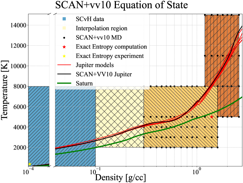
Figure 4: Present work EoS table. Illustrative figure of the different regions that compose our final EoS. At very low $T-\rho$ SCvH data are employed (blue region). In the region between 2000 and 8000 $K$, 0.3 and 1.6 g/cc (orange region) and 5000 to 15000 $K$ and 1.2 to 3.0 g/cc (brown region) MD simulations have been performed in the points highlighted in black. Finally in the region between 2000 and 8000 $K$, 0.1 and 0.3 g/cc (yellow region) an interpolation between SCvH and SCAN+vv10 data has been performed to ensure a smooth connection between the different sources of data. The Jupiter models showed in the figure are taken from [16] for different EoSs. The presence of a small plateau in Jupiter adiabats is due to interior models assuming a change of composition due to helium rain at pressures between 1.64 and 2.12 Mbar. The Saturn model is taken from [112]. We plot in black the Jupiter adiabat obtained using the SCAN+vv10 EoS (see Sect. V)

We seek another independent validation of the SCAN+vv10 functional using the predicted location of the liquid-liquid phase transition as benchmark[98, 63, 31]. The nature and position of the liquid-liquid transition between a molecular, insulating and a atomic, metallic fluid is still debated experimentally. As mentioned previously, DFT predictions heavily depend on the functional chosen, while QMC predictions from different groups are nowadays consistent[32, 31]. Here we demonstrate that the SCAN+vv10 prediction is closer to the QMC line compared to other functionals. While liquid-liquid transition using SCAN have already been reported [58, 59, 101], they used different simulations set-ups and codes. Using a finer grid of densities, we trace the position of the liquid-liquid transition at lower temperatures (i.e. 1000 and 1500 K), i.e. where the transition is expected to exhibit a first-order character. The results, shown in Appendix E, further validate the choice of our SCAN+vv10 set-up as the best EoS for liquid hydrogen. The predicted SCAN+vv10 transition pressure is only about 10 GPa away from the QMC references[32, 31], while PBE differs by about 50 GPa, at 1500 K. Notice that the absolute pressure transitions are $\sim 120$ and $\sim 170$ GPa for PBE and SCAN respectively, such that a difference of 50 GPa is noteworthy. Finally, as mentioned above, it would be tempting to utilize the calculated QMC pressures to construct a fully-QMC EoS; however this would be inaccurate (i.e targeting a sub-GPa accuracy) as the configurations, are sampled at each $\rho$ and $T$ according to weights $e^{-\beta E_{\textrm{PBE}}({\bf x}_{i})}$. In principle, one could adopt a reweighting strategy, where each configuration is weighted with $e^{-\beta(E_{\textrm{VMC}}({\bf x}_{i})-E_{\textrm{PBE}}({\bf x}_{i}))}$. Unfortunately, this estimate is affected by an enhanced statistical error, using only 47 samples for each ($\rho,T$) parameter. Despite this statical noise, the underlying signal is compatible with the SCAN EoS. This corroborates the choice of the SCAN+vv10 functional for hydrogen. The results are shown in Appendix F.

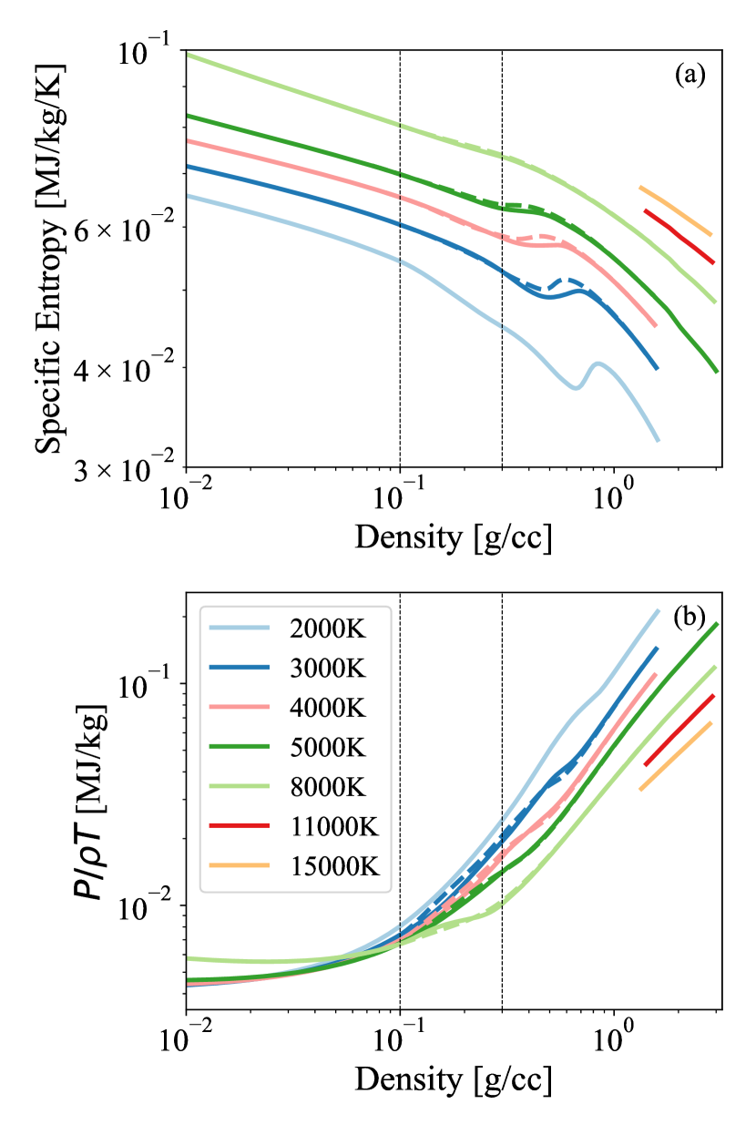
Figure 5: SCAN+vv10 EOS. Several (a) specific entropy, (b) pressure (scaled by $\rho T$) isotherms of our final SCAN+vv10 EoS(solid lines), which consist of the ab initio data at high densities, the SCvH EoS at low densities, and an interpolation region between them, as indicated by the vertical lines. SCAN+vv10 results are compared with PBE results (below 8000 K) from Xie et al. [26] (dashed lines).

IV Calculating the full EoS with entropy

Planetary modeling also requires calculations of entropy. This introduces an additional issue. There has been a longstanding entropy discrepancy between the two most widely used EoS models in planetary science [24, 28], both based on the same PBE electronic structure theory. This conundrum has been recently resolved by some of us in Ref. [26]. The primary source of error was identified as inconsistencies in matching different theories when constructing the EoS table, resulting in an inconsistent thermodynamic construction. Interestingly, the error is not caused by thermodynamic integration over a coarse interpolation grid in $(P,T)$ space, nor due to the linear mixing approximation.

Here, we apply the same methodology to the SCAN data. We interpolate the free energy surface over the ab initio range and then find a smooth connection with the SCvH EOS. The interpolation region is between 0.1 and 0.3 g/cc.

To do so, we perform a rigid shift of the SCvH entropy, as explained in [26]. However, this procedure is not artificial; rather, it ensures that the shifted SCvH EoS matches the room temperature experimental entropy value, that would otherwise be missed by the original SCvH data. The absolute value of the entropy for the ab initio portion of the data, calculated at $5000$ K and $1.4$ g/cc, is $0.0494(2)\,\textrm{MJ/kg/K}$. This value is in agreement with the one calculated at the PBE level (see Ref. [26]). This is expected since at these conditions both PBE and SCAN return the same kind of atomic liquid. Now that we have fixed the two reference entropy points—one at low density and one at high density— we can proceed with the interpolation in the region between the SCvH and the SCAN ab initio data. The results are plotted in Fig. 5.

In Fig. 5, we also directly compare our results with the thermodynamically consistent EoS recently obtained at the PBE level of theory by Xie et. al. [26]. Since we use the same procedure to calculate the entropy, the only differences arise from the use of the SCAN+vv10 functional instead of PBE. This direct comparison allows us to precisely quantify the effect of the xc functional on the EOS. While the difference seems small at this scale, the interior models are very sensitive to changes in thermodynamic properties, such that a few percent difference in the EoS may translate into a much more sizable variation in the model’s predictions (see Sect V).

As expected from the previous section, the main differences occur in the intermediate dissociation region, i.e., from $0.3$ to $1$ g/cc. Entropy exhibits the largest deviations, owing to its strong dependence on molecular dissociation. Notice that we compute the entropy only for $T\geq 2000$ K.

For simplicity, we avoid comparisons with REOS and CSM19 in Fig. 5. Note that both our results and the PBE results of  [26] predict a non-monotonic behavior of entropy in contrast to the CSM19 results. This distinctive entropy behavior implies a flatter Jupiter adiabat (see Sect.  V and Fig. 4).

We also perform additional MD simulations at higher temperatures and densities, compared to the region explored in Sect. III.2. In this way, we cover also the region $5000\leq T\leq 15000$ K, and $1.2\leq\rho\leq 2.6\leavevmode\nobreak\ \textrm{g/cc}$. This region is depicted in brown in Fig. 4. Note also that above $11000$ K we perform finite temperature DFT (using 90 bands) since temperature effects for the electrons may not be neglected anymore. Moreover we switch pseudopotential above $1.8$ g/cc due to the core radius of the SG15-ONCV pseudopotential employed at lower densities. For the simulations in the region $2.0\leq\rho\leq 2.6\leavevmode\nobreak\ \textrm{g/cc}$ we employed ONCV pseudopotential from PseudoDojo library [113] whose smaller core radius allow us to reach a maximum density of $2.7$ g/cc.

Above $8000$ K or about $1$ g/cc, PBE and SCAN+vv10 are very consistent across all quantities. As previously mentioned, the absolute entropies in the fully atomic liquid phase are in agreement.

For all practical purposes, this means that the SCAN+vv10 EoS can be extended to even higher densities and temperatures by matching it to thermodynamically consistent EoSs calculated with PBE. These conditions are needed for modeling the interiors of giant planets like Jupiter. However, H content in the core is much lower compared to the envelope, which contains the majority of the planet’s mass. Residual H-EOS errors in this density regime are therefore expected to have a negligible impact on the models.

In this work, to calculate the interior models of Sect. V, we choose to merge our new SCAN-vv10 EoS with the CMS19 EoS data[27]. An interpolation region is used to smoothly connect the pressure and energy data, while the entropy is recalculated using thermodynamic integration. The initial starting point is selected based on our usual reference condition, at $5000$ K and $1.4$ g/cc, for which we have a precise and accurate absolute entropy evaluation.

The full EoS will be released in tabular form together with the published version of the manuscript.

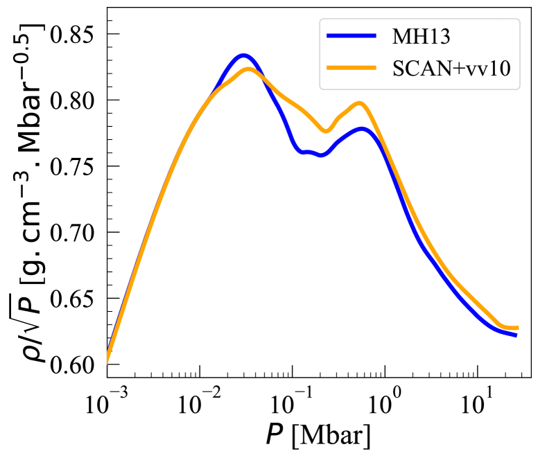
Figure 6: A comparison of the adiabats obtained with our new SCAN+vv10 EoS and the MH13 EoS [24]. Here we used a homogeneous model with no core and a uniform helium composition, starting at $P=1\leavevmode\nobreak\$bar and $T=166.1\leavevmode\nobreak\$K (i.e. Jupiter’s conditions).

V Implications for Jupiter’s interior

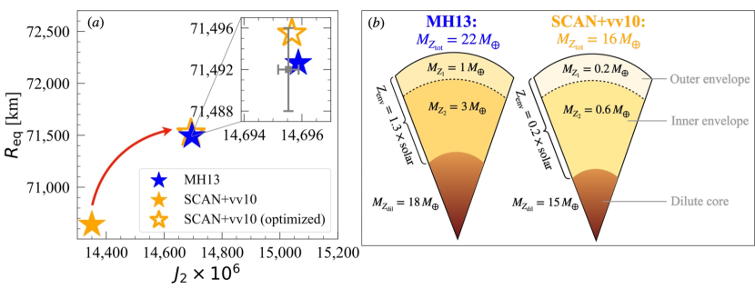
Figure 7: The effect of our new hydrogen EoS on Jupiter’s internal structure. Panel (a) shows the equatorial radius and $J_{2}$ for Jupiter interior models using SCAN+vv10 (orange) or MH13 (blue). The orange empty star shows a model which was optimized to match the observed $R_{\rm eq}$ and $J_{2}$. The grey errorbar shows the observed equatorial radius and the measured $J_{2}$ value accounting for differential rotation (see [17, 16]). Panel (b) shows schematics of Jupiter’s internal structure using the MH13 (left) and SCAN+vv10 (right) EoSs. We show the inferred total heavy-element mass ($M_{Z_{\rm tot}}$) as well as the heavy-element mass in the different layers of the models ($M_{Z_{1}}$, $M_{Z_{2}}$, $M_{Z_{\rm dil}}$) and the envelope metallicity ($Z_{\rm env}$).

In this section, we investigate how the new SCAN+vv10 EoS affects the inferred internal structure and bulk composition of Jupiter. First, we calculated adiabats for pure hydrogen-helium mixtures at Jupiter’s conditions ($T_{\rm 1bar}=166.1\leavevmode\nobreak\$K). We used a simple homogeneous model, without a core and with a uniform helium composition. We assumed linear mixing with mass fractions of hydrogen and helium set at $X=0.755$ and $Y=0.245$, respectively. We compared the adiabat derived from our new EoS for hydrogen, combined with the SCvH-He EoS [22] for helium, to the MH13 EoS [24] which is the current standard for H-He mixtures. The results are shown in Fig. 6. Since $P\propto\rho^{2}$ in Jupiter’s interior [114] we compare values of $\rho/\sqrt{P}$. We find that the differences between the two adiabats are up to 4%. The SCAN+vv10 EoS yields lower densities only between 0.01 and 0.05 Mbar, and higher densities for pressures above 0.05 Mbar (0.01 Mbar $=$ 1 GPa). This is consistent with Fig. 1. Fig. 4 also shows the Jupiter adiabat (in the $\rho-T$ diagram) inferred with our new EOS. Interestingly, its profile is flatter compared to previous models, suggesting a mildly increasing temperature across a large region in the planetary interior. The implication of the new EOS on Jupiter’s composition and thermal profile should be investigated in future studies.

Overall, our new EoS results in a denser adiabat throughout most of Jupiter’s interior. This implies that interior models using the new EoS will yield lower metallicities (less heavy elements). This is because if the density of hydrogen is higher, in order to fit a given density (which is consistent with the gravity data), less heavy elements can be included.

To determine the differences in the inferred bulk composition of Jupiter with the new EoS, we used a Jupiter model from [16] based on the MH13 EoS (see their Table E.1.). This model assumes the presence of a dilute core, helium differentiation between an outer envelope of molecular hydrogen and an inner envelope of metallic hydrogen, with a high internal entropy (see e.g., [14] for further details). Note that the heavy-element mass fraction (i.e., the envelope metallicity) is assumed to be the same in the inner and outer envelopes. The left panel of Figure 7 shows the inferred equatorial radius and $J_{2}$ for the Jupiter model with the MH13 EoS (blue star). Using CEPAM [115], we calculated a similar Jupiter model with SCAN+vv10 (orange star). Due to the higher densities predicted by our EoS, we obtain a smaller radius and a lower $J_{2}$ value. In order to match Jupiter’s observed equatorial radius and $J_{2}$, we adjust the extent of the dilute core and the heavy-element mass fraction in the envelope ($Z_{\rm env}$). The results for Jupiter’s internal structure are shown in the right panel of Figure 7. We find that: (i) the required modification of the extent of the dilute core decreases the heavy-element mass in this region from $M_{Z_{\rm dil}}=18\leavevmode\nobreak\ M_{\oplus}$ to $15\leavevmode\nobreak\ M_{\oplus}$, and (ii) the envelope metallicity $Z_{\rm env}$ decreases from $1.3\times\rm solar$ to $0.2\times\rm solar$. The heavy-element mass in the outer envelope is reduced from $M_{Z_{1}}=1\,M_{\oplus}$ to $0.2\,M_{\oplus}$ and in the inner envelope from $M_{Z_{2}}=3\,M_{\oplus}$ to $0.6\,M_{\oplus}$.

Overall, using SCAN+vv10 rather than MH13 led to a decrease in the inferred total heavy-element mass in Jupiter, from $M_{Z_{\rm tot}}=22\leavevmode\nobreak\ M_{\oplus}$ to $16\leavevmode\nobreak\ M_{\oplus}$. Note that although our results correspond to a single optimized model, the trend of lower inferred metallicity for Jupiter using the SCAN+vv10 EoS is robust due to the higher inferred density of hydrogen at Jupiter’s conditions.

Our study suggests that the tension between Jupiter’s atmospheric metallicity as measured by the Galileo probe and the metallicity inferred by interior models remains, and in fact, with the new EoS the difference between the two values increases. While the Galileo probe measured an atmospheric metallicity of three times solar, our presented Jupiter model predicts an atmospheric metallicity of 0.2 solar, a difference by a factor of 15! It is therefore clear that the discrepancy between Jupiter’s atmosphere and interior metallicities cannot be resolved by improvements in the hydrogen EoS calculations.

VI Conclusion

We calculate the equation of state for hydrogen using a more accurate electronic structure method compared to currently adopted EoSs,[28, 24, 27, 47] validated against computationally intensive quantum Monte Carlo calculations (these alone utilized 82 million CPU hours). Several density functional theories have been tested, and we identified SCAN+vv10 as the consistently best-performing setup. In addition, we find that other reasonable and previously adopted functionals for hydrogen yield EoSs that vary by up to $\pm 20\%$, significantly exceeding the accuracy required for constructing planetary models. Therefore, benchmarking against a higher level of theory is crucial to avoid qualitatively incorrect predictions. We also find that the PBE functional, which forms the basis of currently utilized EoSs, does not perform excessively poorly. However, this result is likely fortuitous, as PBE significantly underestimates the metallization pressure by about $25\%$ and produces inaccurate molecular bond predictions.[54]

The new EoS is derived from first principles and is thermodynamically consistent across a wide range of densities and temperatures. Since knowledge of the hydrogen EoS is critical for determining Jupiter’s internal structure, we also explored how our new EoS affects the predicted composition and internal structure of the planet. Because the SCAN+vv10 hydrogen EoS is denser, it leads to a lower bulk metallicity for Jupiter. The lower inferred envelope metallicity in Jupiter further highlights the mismatch between the enrichment of Jupiter’s atmosphere as measured by the Galileo probe and the one inferred from structure models. Although there were speculations that this disagreement could be resolved by improvements in the hydrogen EoS calculations [116], our study shows that this is not the case. We therefore conclude that this inconsistency cannot be resolved by improving the uncertainties in the hydrogen EoS. Instead, it implies that the internal structure of Jupiter is more complex than typically assumed and that the atmospheric composition does not represent the bulk composition. It is therefore possible that Jupiter’s outmost atmospheres is more metal-rich than its outer envelope [117, 118, 119]. This conclusion is of high importance for the interpretation of atmospheric measurements of giant planets’ atmospheres in the solar system and around other stars. Finally, our modified hydrogen EoS will also affect the inferred bulk compositions of Saturn and giant exoplanets and we hope to address this in future research.

Appendix A Details of DFT calculations

All the DFT simulations have been performed using QuantumESPRESSO [120], with plane-wave basis set and $3\times 3\times 3$ Monkhorst-Pack grid for the k-points. For BLYP, PBE, PBEsol, vdW-DF, vdW-DF2, vdW-DF2-c09 xc functionals it has been used projected-augmented-wave (PAW) pseudopotentials [121] from psl library [122]; all the other xc functionals employ optimized norm-conserving Vanderbilt (ONCV) pseudopotentials [123] from the SG15 library [124].
For every xc functional the kinetic energy cutoffs for both the wavefunction and density have been studied through convergence of the internal energy and stresses, and the consistency between numerical and analytical pressure is checked as explained in Appendix D. All the xc functional using PAW pseudopotential have been employed with a wavefunction cutoff of 80 Ry and a density cutoff of 800 Ry. The hybrid functionals (i.e. HSE and PBE0) and rVV10 employ 100 and 400 Ry for the wavefunction and density cutoff respectively, moreover for HSE and PBE0 it has been employed a kinetic energy cutoff for the exact exchange operator of 100 Ry and a $1\times 1\times 1$ three-dimensional mesh for q sampling of the Fock operator. The meta-GGA xc functionals (i.e. SCAN, rSCAN, etc.) requires an higher wavefunction cutoff, due to their additional dependence on the kinetic energy density, of 140 Ry and 560 Ry for the density cutoff. It has been tried to increase just the FFT grid as suggested in Ref.[125], but it did not provide the converged results. For all the SCANs functional a pseudopotential generated with SCAN xc has been tried [125], it has been tested on a smaller set of configurations (10 configuratiions for every $T-\rho$) providing results that are slightly better than the same functional with a PBE pseudopotential. Nevertheless the SCAN pseusopotential requires a wavefunction and density cutoff of 280 and 1120 Ry to reach convergence, respectively, and the improvement in the results is not enough to justify a doubling in the computational time.
The Molecular Dynamics simulations with PBE xc functionals, used to sample the configurations for the benchmark against QMC have been performed with over damped Langevin dynamics with timestep ranging from 0.2 to 0.05 a.u. depending from $T-\rho$. The same set up has been used for the vdW-DF2 and PBEsol MD. The SCAN+vv10 MD has been performed using Stochastic Velocity Rescaling (SVR) thermostat [126], with timestep ranging from 2 to 21 a.u. (0.1 to 1 fs) depending from $T-\rho$.

The PAW and ONCV pseudopotentials used in this study were very carefully validated via the comparison with all-electron DFT calculations performed by Vienna Ab initio Simulation Package (VASP) code [127]. In all electron calculations by VASP, the kinetic energy cutoff was set to 10000 eV. The same smearing method, smearing parameter, and k-point were employed. Figure 8 shows pressures computed by QuantumESPRESSO with the PAW pseudo potential and those computed by all-electron calculations using VASP, where LDA-PZ functional was employed. They give perfectly consistent pressures, indicating that the use of the PAW pseudo potential does not introduce bias. Figure. 8 shows pressures computed by QuantumESPRESSO with the PAW pseudo potential and those computed by QuantumESPRESSO with the ONCV pseudo potential, where GGA-PBE functional was employed. They give perfectly consistent pressures, indicating that the use of the ONCV pseudo potential does not introduce bias.

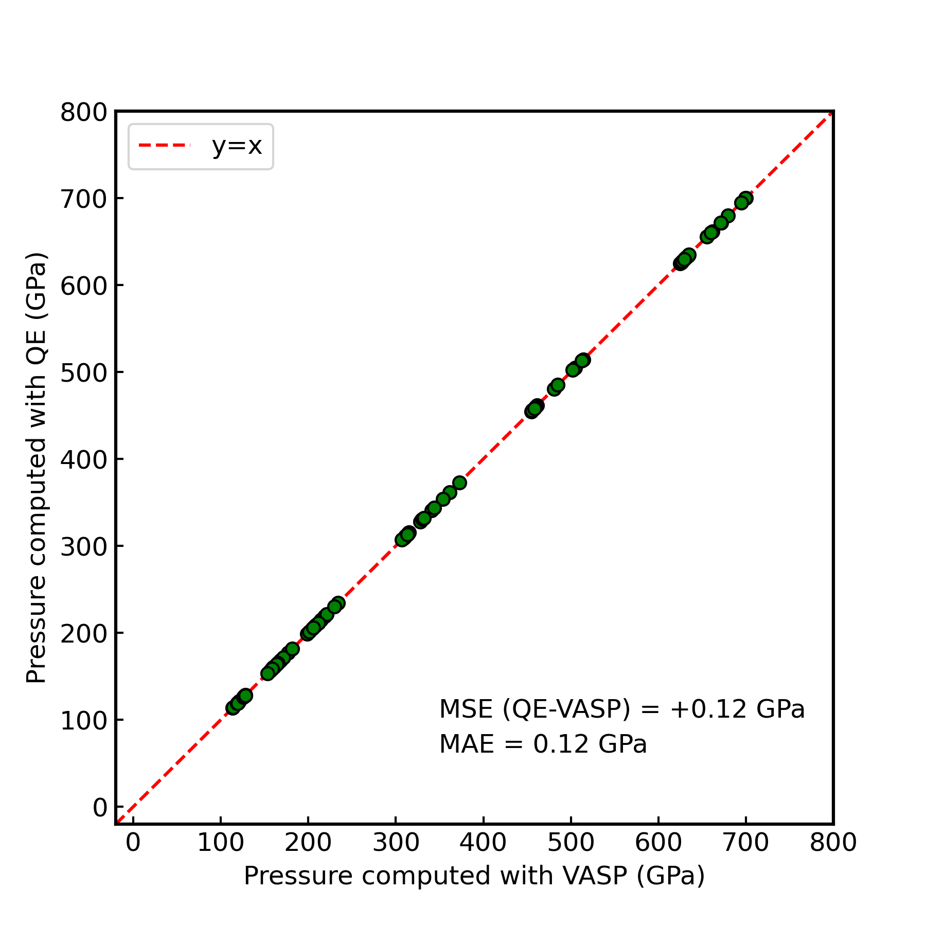
Figure 8: The comparison between pressures computed by QuantumESPRESSO with the PAW pseudo potential and those computed by all-electron calculations using VASP. The LDA-PZ functional was employed. MSE and MAE stand for mean signed error and mean absolute error, respectively.

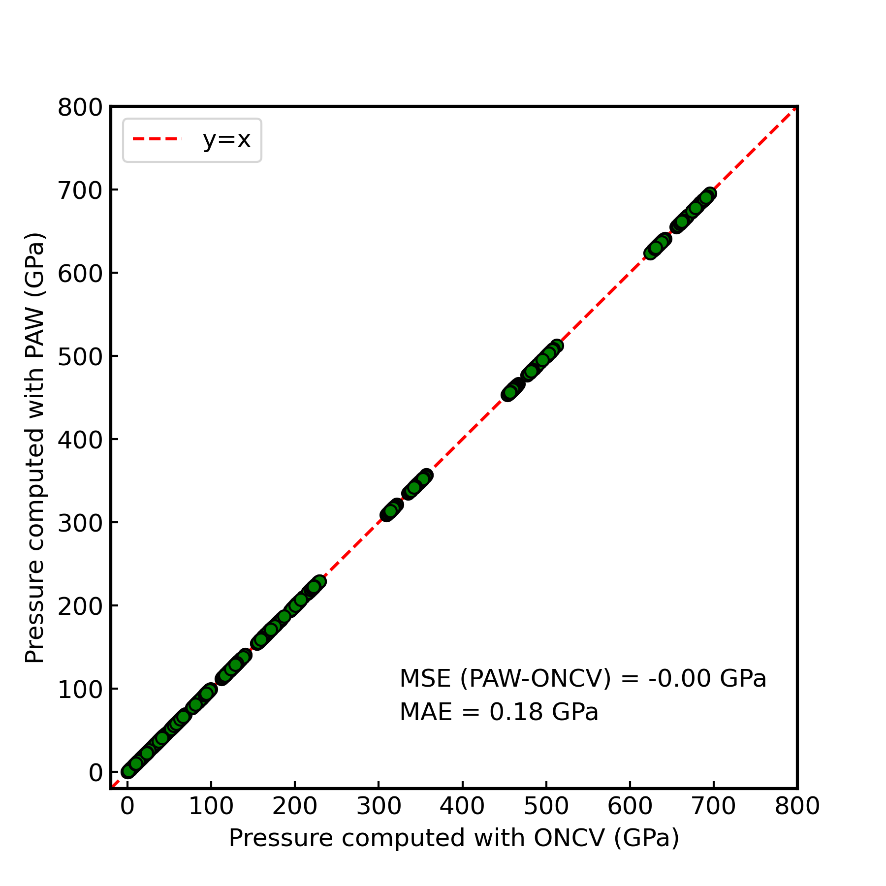
Figure 9: The comparison between pressures computed by QuantumESPRESSO with the PAW pseudo potential and those computed by QuantumESPRESSO with the ONCV pseudo potential. The GGA-PBE functional was employed. MSE and MAE stand for mean signed error and mean absolute error, respectively.

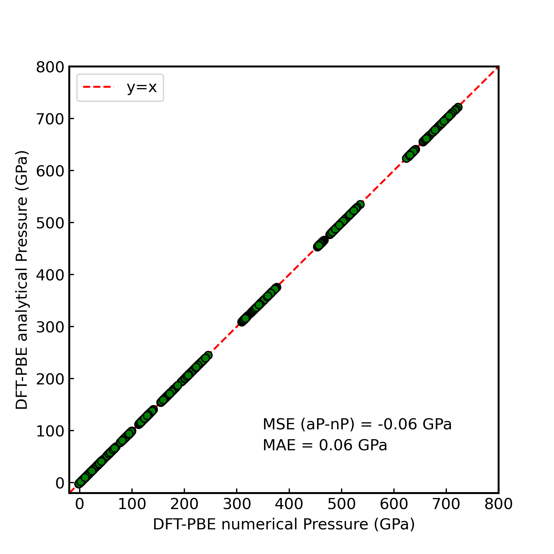
Figure 10: The comparison between pressures computed by QuantumESPRESSO via FDM (denoted as nP:numerical pressure) and those computed via the Hellmann–Feynman theorem (denoted as aP:analytical pressure). The GGA-PBE functional and the PAW pseudo potential were employed. MSE and MAE stand for mean signed error and mean absolute error, respectively.

Appendix B Details of VMC and LRDMC calculations

The all-electron VMC and LRDMC calculations for the liquid hydrogen were performed using TurboRVB [72] combined with the Python package TurboGenius [76]. TurboRVB employs the Jastrow antisymmetrized geminal power (JAGP) [128] ansatz. The ansatz is composed of a Jastrow and an antisymmetric part ($\Psi=J\cdot{\Phi_{{\text{AGP}}}}$). The singlet antisymmetric part is denoted as the singlet antisymmetrized geminal power (AGPs), which reads:

$${\Psi_{{\text{AGPs}}}}\left({{{\mathbf{r}}_{1}},\ldots,{{\mathbf{r}}_{N}}}\right)=$$

$${\hat{A}}\left[{\Phi\left({{\mathbf{r}}_{1}^{\uparrow},{\mathbf{r}}_{1}^{\downarrow}}\right)\Phi\left({{\mathbf{r}}_{2}^{\uparrow},{\mathbf{r}}_{2}^{\downarrow}}\right)\cdots\Phi\left({{\mathbf{r}}_{N/2}^{\uparrow},{\mathbf{r}}_{N/2}^{\downarrow}}\right)}\right],$$ (11)

where ${\hat{A}}$ is the antisymmetrization operator, and $\Phi\left({{\mathbf{r}}^{\uparrow},{\mathbf{r}}^{\downarrow}}\right)$ is called the pairing function. The spatial part of the geminal function is expanded over the Gaussian-type atomic orbitals (GTOs):

$${\Phi_{{\text{AGPs}}}}\left({{{\mathbf{r}}_{i}},{{\mathbf{r}}_{j}}}\right)=\sum\limits_{l,m,a,b}{{f_{\left\{{a,l}\right\},\left\{{b,m}\right\}}}{\psi_{a,l}}\left({{{\mathbf{r}}_{i}}}\right){\psi_{b,m}}\left({{{\mathbf{r}}_{j}}}\right)},$$ (12)

where ${\psi_{a,l}}$ and ${\psi_{b,m}}$ are primitive GTOs, their indices $l$ and $m$ refer to different orbitals centered on atoms $a$ and $b$, and $i$ and $j$ are coordinates of spin-up and spin-down electrons, respectively. When the JAGPs is expanded over $p$ = $N_{\rm el}/2$ molecular orbitals, the JAGPs coincides with the Jastrow–Slater determinant (JSD) ansatz. In this study, we restrict ourself to use the JSD anstaz. Indeed, the coefficients in the pairing functions (i.e., variational parameters in the antisymmetric part) are obtained by the built-in DFT code, named Prep, with the PZ-LDA functional and the coefficients are fixed during the VMC optimization step. This is the simplest choice, but it is reasonable in the majority of QMC applications. Only the coefficients in the Jastrow factor are optimized at the VMC level, which keeps the nodal surface of the trial wavefunction unchanged from that obtained at the DFT level. Indeed, the LRDMC calculations were done using the DFT nodal surfaces (i.e., the JSD ansatz with the DFT nodal surfaces).

The Jastrow term is composed of one-body, two-body, and three-body factors ($J={J_{1}}{J_{2}}{J_{3}}$). The one-body and two-body factors are used to satisfy the electron–ion and electron–electron cusp conditions, respectively, and the three-/four-body factor is adopted to take the further electron–electron correlation into consideration. The one-body Jastrow factor reads:

$${J_{1}}\left({{{\mathbf{r}}_{1}},\ldots,{{\mathbf{r}}_{N}}}\right)=\exp\left({\sum\limits_{i,I,l}{g_{I,l}\chi_{I,l}\left({{{\mathbf{r}}_{i}}}\right)}}\right)\cdot\prod\limits_{i}{{{\tilde{J}}_{1}}\left({{{\mathbf{r}}_{i}}}\right)},$$ (13)

where

$${\tilde{J}_{1}}\left({\mathbf{r}}\right)=\exp\left({\sum\limits_{I}{-{{\left({2{Z_{I}}}\right)}^{3/4}}u\left({2{Z_{I}}^{1/4}\left|{{\mathbf{r}}-{{\mathbf{R}}_{I}}}\right|}\right)}}\right),$$ (14)

${{{\mathbf{r}}_{i}}}$ are the electron positions, ${{{\mathbf{R}}_{I}}}$ are the atomic positions with corresponding atomic number $Z_{I}$, $l$ runs over atomic orbitals ${\chi_{I,l}^{J}}$ centered on atom $I$, and ${u\left(r\right)}$ is a short-range function containing a variational parameter $b$:

$$u\left(r\right)=\frac{b}{2}\left({1-{e^{-r/b}}}\right).$$ (15)

The two-body Jastrow factor is defined by a long-range function as:

$${J_{2}}\left({{{\mathbf{r}}_{1}},\ldots,{{\mathbf{r}}_{N}}}\right)=\exp\left({\sum\limits_{i<j}{v\left({\left|{{{\mathbf{r}}_{i}}-{{\mathbf{r}}_{j}}}\right|}\right)}}\right),$$ (16)

where $v\left(r\right)$ is:

$$v\left(r\right)=\frac{1}{2}r\cdot{\left({1+F\cdot r}\right)^{-1}}$$ (17)

and $F$ is a variational parameter. The three-body Jastrow factors are:

$${J_{3}}\left({{{\mathbf{r}}_{1}},\ldots,{{\mathbf{r}}_{N}}}\right)=\exp\left({\sum\limits_{i<j}{{\Phi_{{\text{Jas}}}}\left({{{\mathbf{r}}_{i}},{{\mathbf{r}}_{j}}}\right)}}\right),$$ (18)

and

$${\Phi_{{\text{Jas}}}}\left({{{\mathbf{r}}_{i}},{{\mathbf{r}}_{j}}}\right)=\sum\limits_{l,m,a}{g_{l,m,a}\chi_{a,l}^{{\text{Jas}}}\left({{{\mathbf{r}}_{i}}}\right)\chi_{a,m}^{{\text{Jas}}}\left({{{\mathbf{r}}_{j}}}\right)},$$ (19)

where the indices $l$ and $m$ again indicate different orbitals centered on corresponding atoms $a$.

In the antisymmetric part, the uncontracted cc-pVTZ basis set [4$s$2$p$1$d$] taken from the Basis-Set Exchange Library [129] modified with the one-body Jastrow factor [31] were employed. This is the same one used in previous high-pressure hydrogen studies [89, 83, 130]. Moreover, Mazzola et al., reported that the modified cc-pVTZ basis was converged to the CBS limit (within 0.01 eV/atom) [31]. Hereafter, we describe the detail of the modification of the one-body orbitals. The original basis set was modified such that the $s$ orbitals whose exponents are larger than $8\cdot Z^{2}$ (where $Z$ is the atomic number) are disregarded, and they are implicitly compensated by the homogeneous one-body Jastrow part [${\tilde{J}_{1}}\left({\mathbf{r}}\right)$] to fulfill the electron–ion cusp condition explicitly [31, 131]. Indeed, a single-particle orbital is modified as:

$$\tilde{\phi}_{j}^{b}\left({{\mathbf{r}}-{{\mathbf{R}}_{b}}}\right)=\phi_{j}^{b}\left({{\mathbf{r}}-{{\mathbf{R}}_{b}}}\right){{\tilde{J}}_{1}}\left({\mathbf{r}}\right),$$ (20)

where ${{\tilde{J}}_{1}}\left({\mathbf{r}}\right)$ is the same as in Eq. (14). The parameter $b$ in Eq. (15) is set to 1.1 for all volume points, and optimized at the VMC level. In this way, each element of the modified basis set satisfies the electron–ion cusp conditions even at the DFT level [31, 131].

In the inhomogeneous one-body and three-body Jastrow parts, [2$s$2$p$1$d$] basis set was employed, which is the same basis set as used in recent high-pressure hydrogen studies [83, 130]. The variational parameters in the Jastrow factors were optimized the Stochastic Reconfiguration method described in Refs. [81, 82] implemented in TurboRVB.

The LRDMC calculations for computing the PESs were performed by the single-grid scheme [75] with the lattice space $a$ = 0.30 Bohr. For several structures, we performed LRDMC calculations with the lattice space $a$ = 0.20 Bohr and confirmed that the obtained pressures are consistent with those obtained with the lattice space $a$ = 0.30 Bohr within their statistical uncertainties (within $2\sigma$).

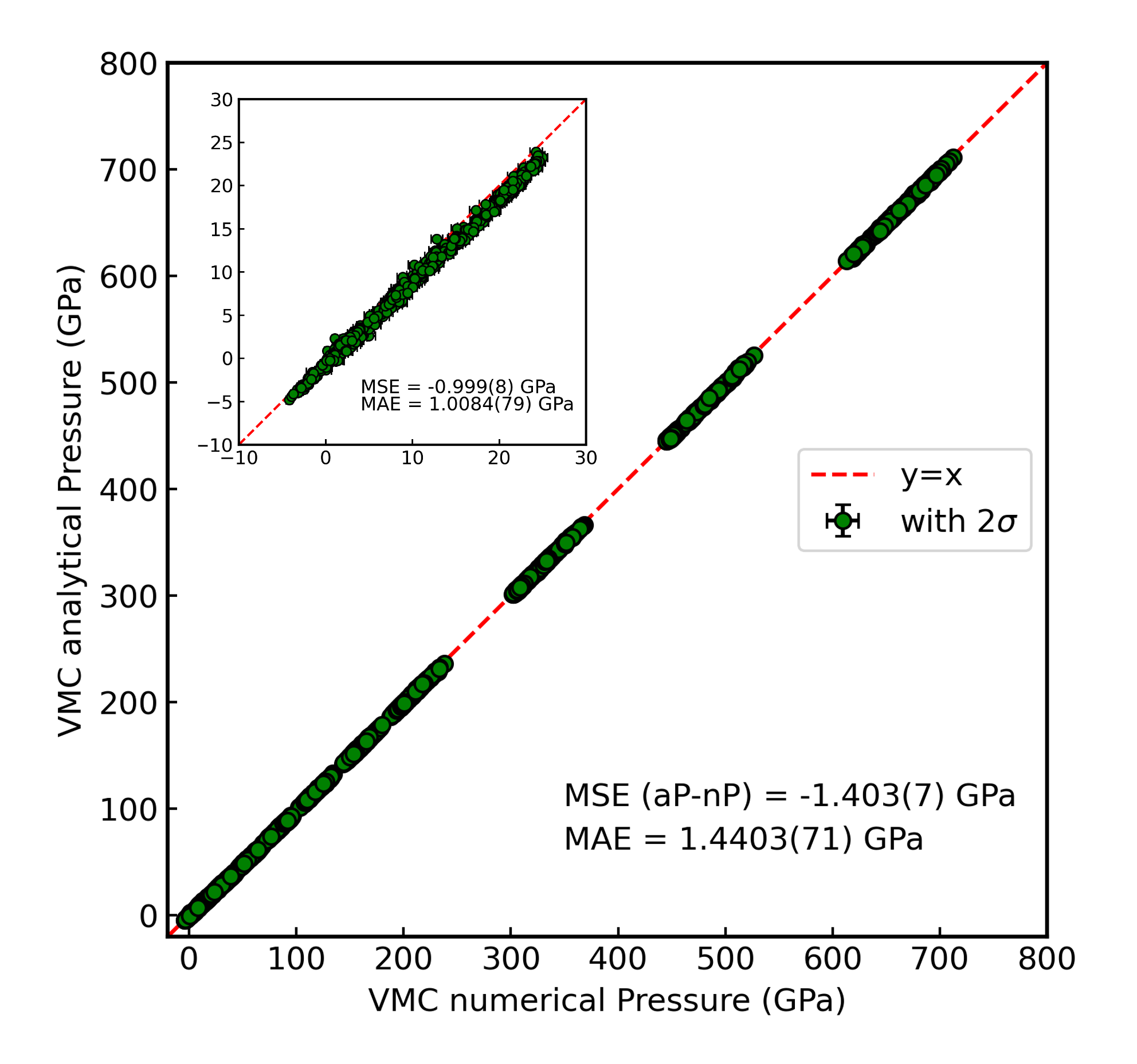
Figure 11: The comparison between Pressures computed via FDM (denoted as nP: numerical pressure) and those computed from the Hellmann–Feynman and Pulay terms (denoted as aP:analytical pressure) at the VMC level. Inset: Those in the range $\leq$ 25 GPa. MSE and MAE stand for mean signed error and mean absolute error, respectively.

Appendix C Difficulty in Computing Unbiased Atomic forces and Pressures by QMC

Although the computation of atomic forces and pressures are established and routinely used in the DFT framework, they are still under development in QMC calculations [132, 133, 134, 135, 136, 137, 138, 139, 103, 104, 92]. There are three routes to compute unbiased forces and pressures. (i) fitting potential energy surfaces with respect to an atomic position or the volume (a.k.a. finite-difference method: FDM). (ii) computing the so-called Hellmann–Feynman and Pulay terms with a fully optimized WF. (iii) computing the Hellmann–Feynman and Pulay terms with a partially optimized WF and compensating the missing term appearing with the partially optimized WF. (i) is the most straightforward computation and is applicable both for VMC and LRDMC calculations, and is the one adopted in this study. The significant drawback of this approach is that the computation of atomic forces is infeasible for large systems because 3$N_{a}$ times FDM fitting procedures are needed, where $N_{a}$ refers to the number of atoms in the system. Therefore, we computed only pressures and used them as reference data for bench-marking XC functionals. (ii) has been successful for small molecules and solids [104, 130, 140], while it is impractical in this study because the number of variational parameters is too much to exactly optimize all of them. (iii) Nakano et al. [92] recently proposed a method that guarantees unbiased forces and pressures even though not all variational parameters are optimized. Their proposed method have been successful for VMC force and pressure computations, while it is still under development for DMC forces and pressures.

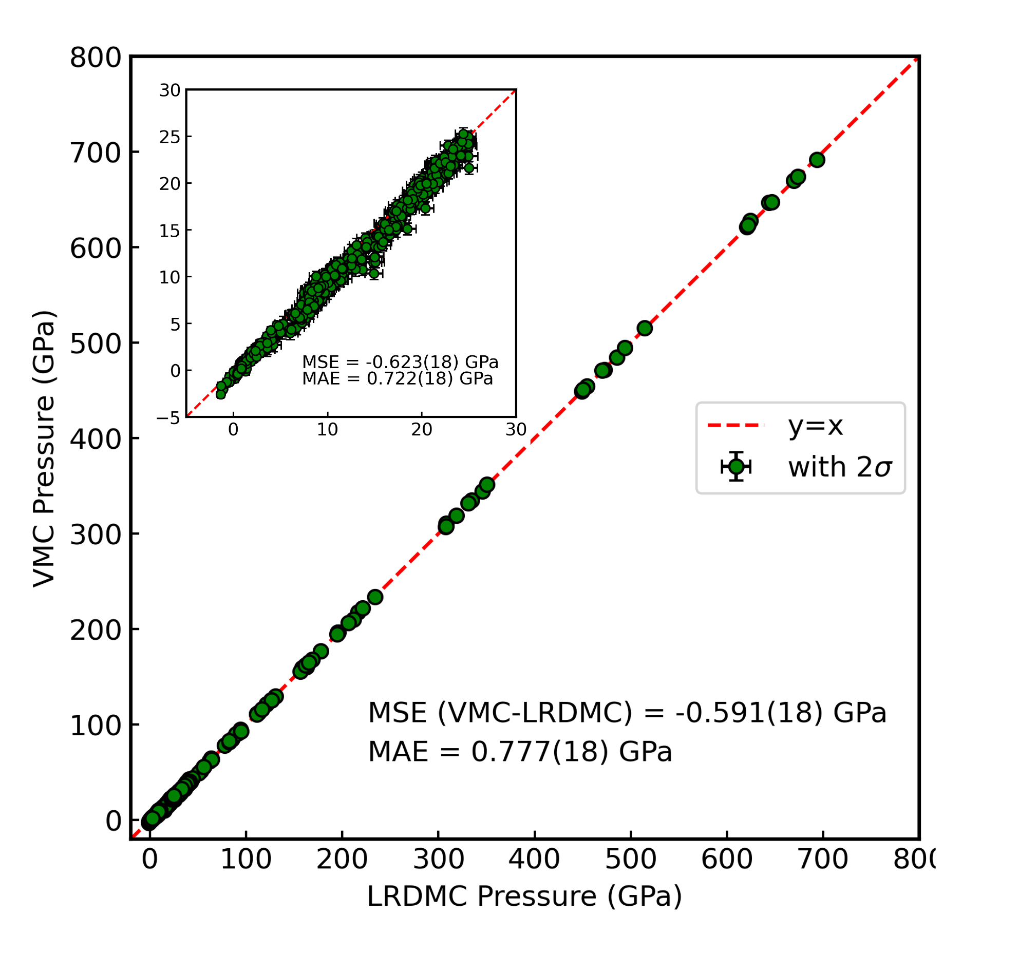
Figure 12: The comparison between Pressures computed by VMC and LRDMC. Inset: Those in the range $\leq$ 25 GPa. MSE and MAE stand for mean signed error and mean absolute error, respectively.

Appendix D Validation of the VMC and LRDMC setups for computing pressures.

The VMC and LRDMC pressures were computed by fitting energy curves computed with 7 volumes ($r_{s}$) around the target one. The fittings were done using the third-order polynominal function. First of all, using DFT, we confirmed that the chosen polynomial enables us to compute pressures correctly. More specifically, since the aforementioned bias problem does not exist in DFT, the pressures obtained via the PES fitting (denoted as numerical pressure) and those directly obtained via the Hellmann–Feynman theorem (denoted as analytical pressure) should be perfectly consistent. Figure 10 shows the consistency checks for the randomly chosen configurations in the entire density region. The figure clearly shows that the fitting with the third-order polynomial gives pressures perfectly consistent with those directly obtained via the Hellmann–Feynman theorem. We also confirmed that all the PES obtained by VMC and LRDMC calculations are as smooth as those in the DFT calculations, thanks to accumulated statistics (In the VMC calculations, $\sim 1.2$ mHa/cell and $\sim 1.0$ mHa/cell for $r_{s}\leq 2.079$ and $r_{s}=2.380$, respectively. In the LRDMC calculations, $\sim 2.0$ mHa/cell and $\sim 1.2$ mHa/cell for $r_{s}\leq 2.079$ and $r_{s}=2.380$, respectively).

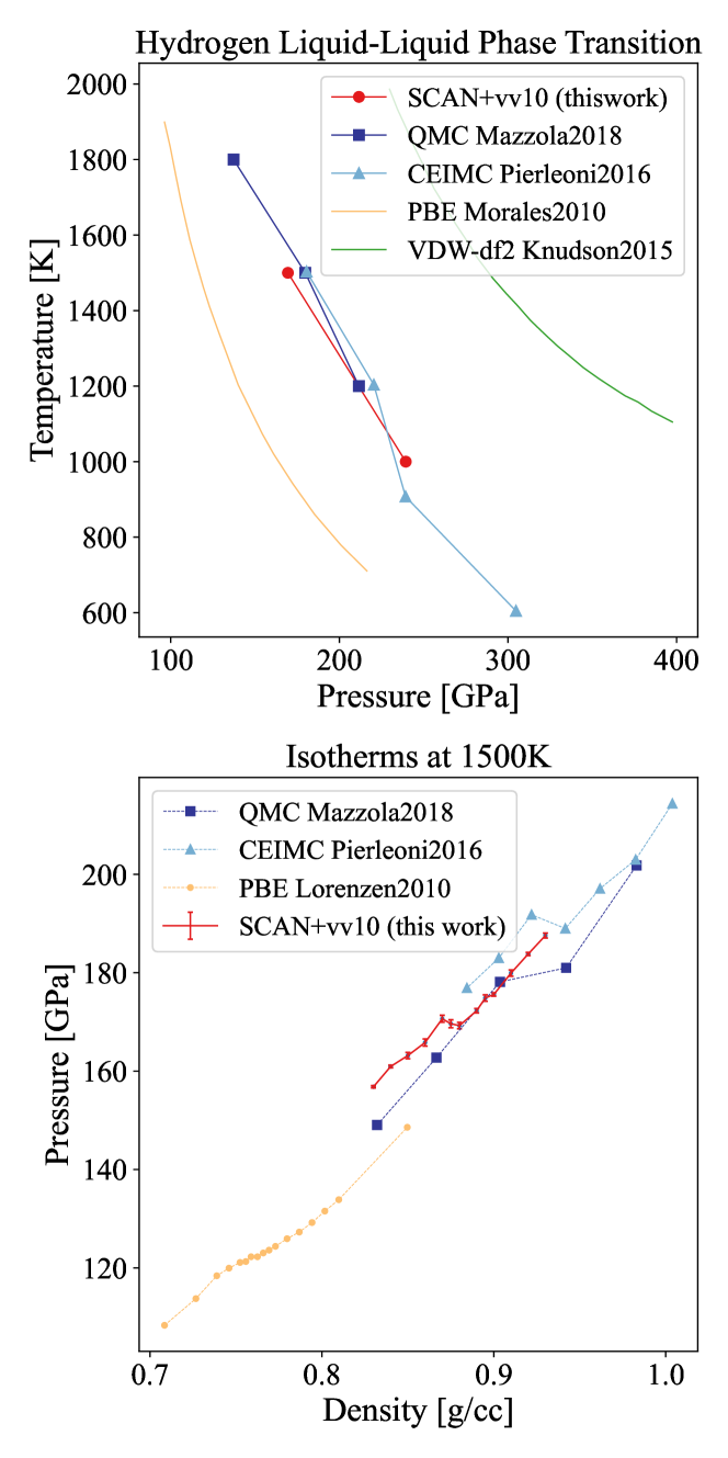
Figure 13: Liquid-liquid phase transition obtained with our SCAN+VV10 ab-initio. Top: Location of the phase boundary in the $P,T$ plane. We also plot the predictions made using PBE [98], vdW-DF2[10] and QMC, using the CEIMC method[32] and a VMC-MD method which uses the same VMC code as the present work and but a slighlty different set-up[31]. Bottom: the discontinuity of the EoS at 1500 K from the different theories. We chose to plot the 1500 K isotherm as we can find published data, from the above references, for this exact temperature.

Figure 11 plots the numerical and analytical VMC pressures collected from all 4512 configurations. The figure reveals that the biased arising from the parameters which are not variationally minimum amounts to MAE = $\sim$ 1.440(7) GPa, which is constant among the studied $P$ and $r_{s}$, highlighting the importance in the smaller P and $r_{s}$ region. Fig. 12 plots numerical (i.e. unbiased) VMC and LRDMC pressures collected from 832 configurations. The figure reveals that LRDMC and VMC pressures are consistent in the concerned pressure region (MAE = $\sim$ 0.78(2) GPa and $\sim$ 0.72(2) GPa for all $P$ and for $P\leq 25$ GPa, respectively), supporting the reliability our XC benchmark test referring to VMC Pressures as thier reference values.

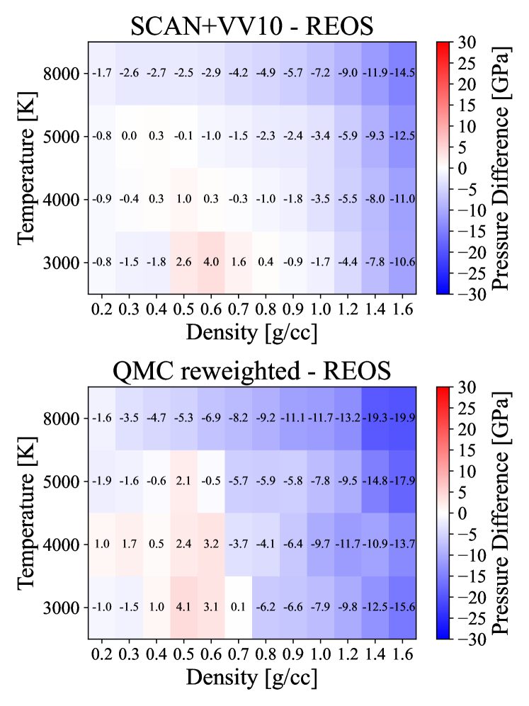
Figure 14: Comparison between the QMC EoS obtained by reweighting method (Eq. 21) and the SCAN EoS, for $T\geq 3000K$. Shown is the difference with REOS.

Appendix E Liquid-liquid phase transition

In Fig. 13 we show the agreement of SCAN+VV10 with previously published QMC data concerning the location of the liquid-liquid phase transition. It is important to mention that all simulations reported adopt the classical-ions approximations as we do in the main text. At about 1000 K nuclear quantum effects are expected to push the transition to lower pressure by about 30 GPa, therefore one needs to be careful to not mix data with and without inclusion of zero-point motion.

Appendix F Reweighting technique

In principle, it could be possible to compute average values for different level of theories, using only one configuration dataset $\bar{\bf x}_{\alpha}$, e.g. computing $\langle O\rangle_{B}$ without running a full MD at theory $B$, but postprocessing the set $\bar{\bf x}_{A}$ using a procedure called reweighting. Formally, the expectation value of an operator $O$ can be computed using

$$\langle O\rangle_{B}=\frac{1}{M}\sum_{{\bf x}_{i}\in\bar{\bf x}_{A}}O_{B}({\bf x}_{i})\omega_{A\rightarrow B}({\bf x}_{i}),$$ (21)

where

$$\omega_{A\rightarrow B}({\bf x}_{i})=\frac{e^{-\beta(E_{B}({\bf x}_{i})-E_{A}({\bf x}_{i}))}}{\sum_{{\bf x}_{i}\in\bar{\bf x}_{A}}e^{-\beta(E_{B}({\bf x}_{i})-E_{A}({\bf x}_{i}))}}\quad.$$ (22)

With this procedure one enhance or decrease the significance for of a datapoint ${\bf x}_{i}$ sampled with theory $A$, for the theory $B$. Unfortunately this procedure is unstable, due to the large fluctuation of the weights, as the energy $E$ is an extensive quantity. Clearly, the fluctuations are particularly severe at low temperature, due to the presence of the inverse temperature in the exponents. The method becomes more accurate as the energy predicted by the two theories becomes equal.

We can try this procedure using $A=$ PBE and $B=$ VMC. In Fig. 14 we plot the reweighted VMC pressure on the PBE configurations, and we compare with the SCAN+VV10 EoS. For consistency we plot the differences with respect of REOS3. We also plot only the region above 2000 K because it is less affected by statistical noise and is relevant for planetary science.

We notice that the two EoS are qualitative in agreement, both showing a region at intermediate densities where they predicts a lighter liquid compared to REOS, while it is denser at higher densities. However, the statistical error of this method is of about 8 GPa. For this reason the VMC reweighted results cannot be used to build a precise EOS, but the signal it provides us is a further proof of the quality of the SCAN+VV10 results. Notice that statistical noise in the EoS would prevent us from calculating entropy accurately.

Appendix G Extended DFTxc benchmarks

In the following we show the results for the benchmark against VMC and LRDMC for energy and pressure for all the DFT xc functional s who has been tested.

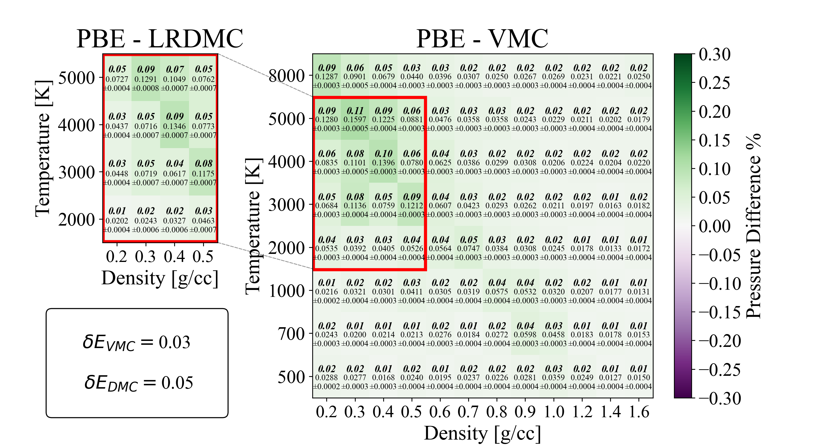
(a)

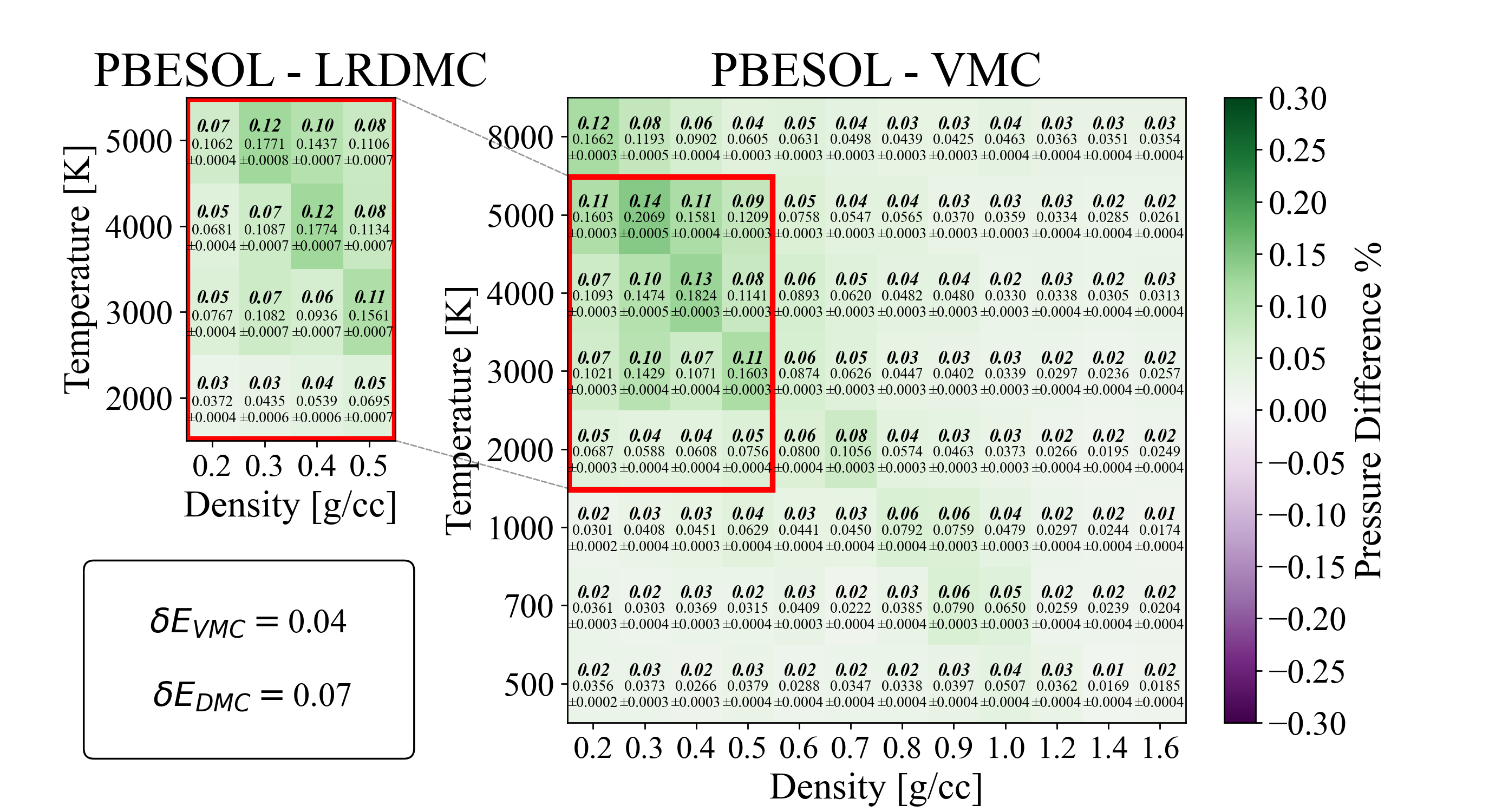
(b)

(c)

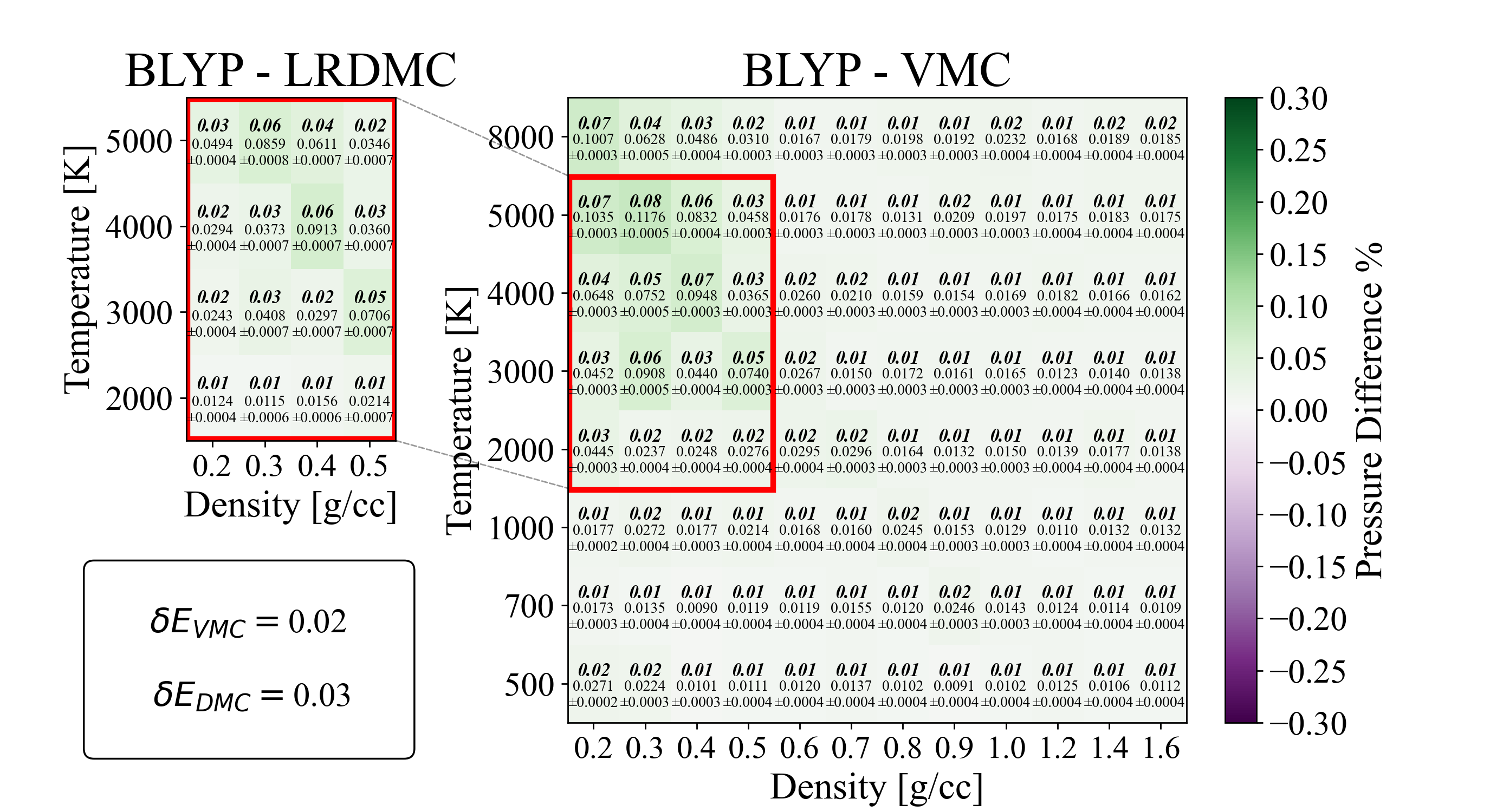
(d)

(e)

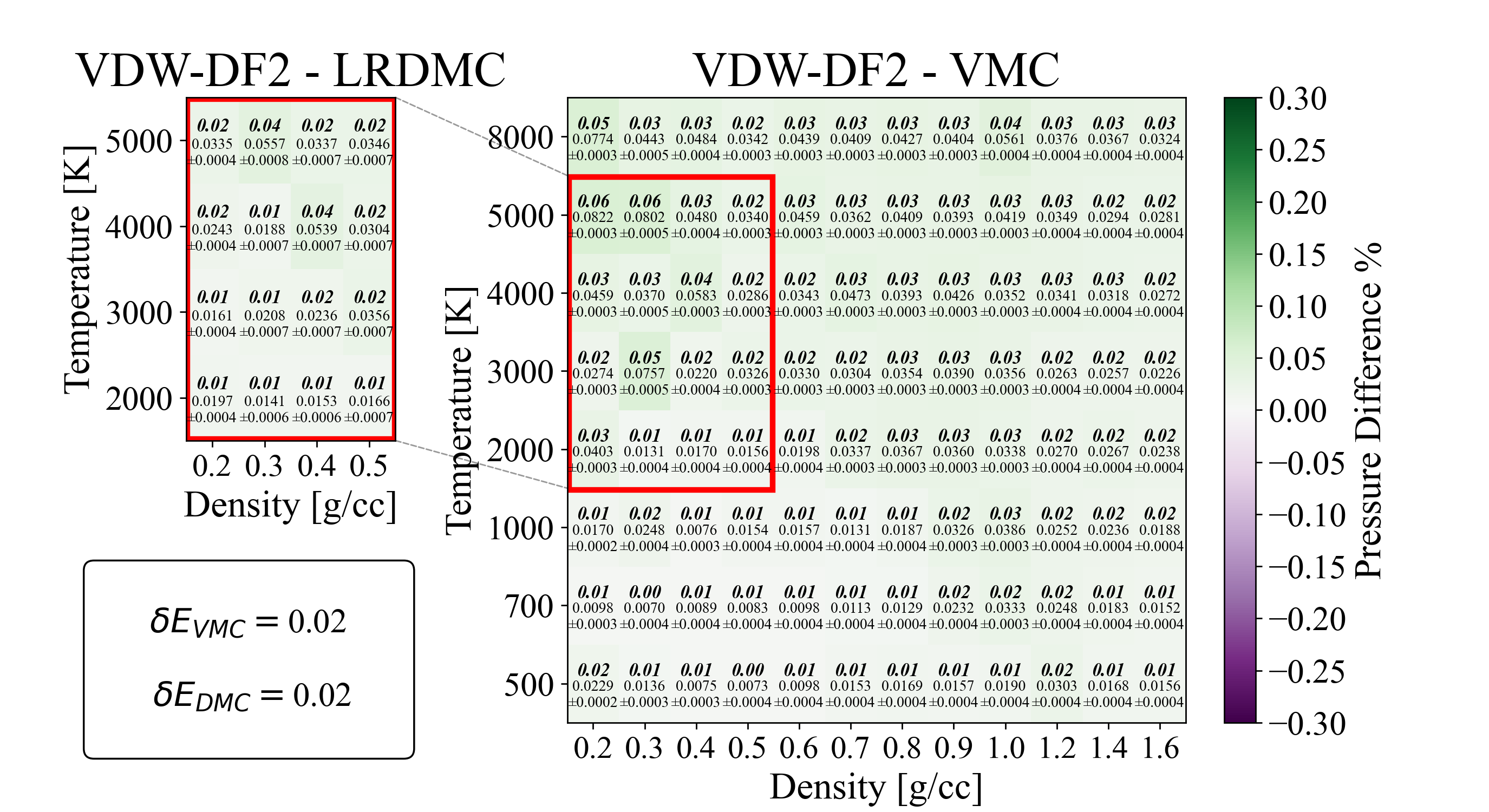
(f)

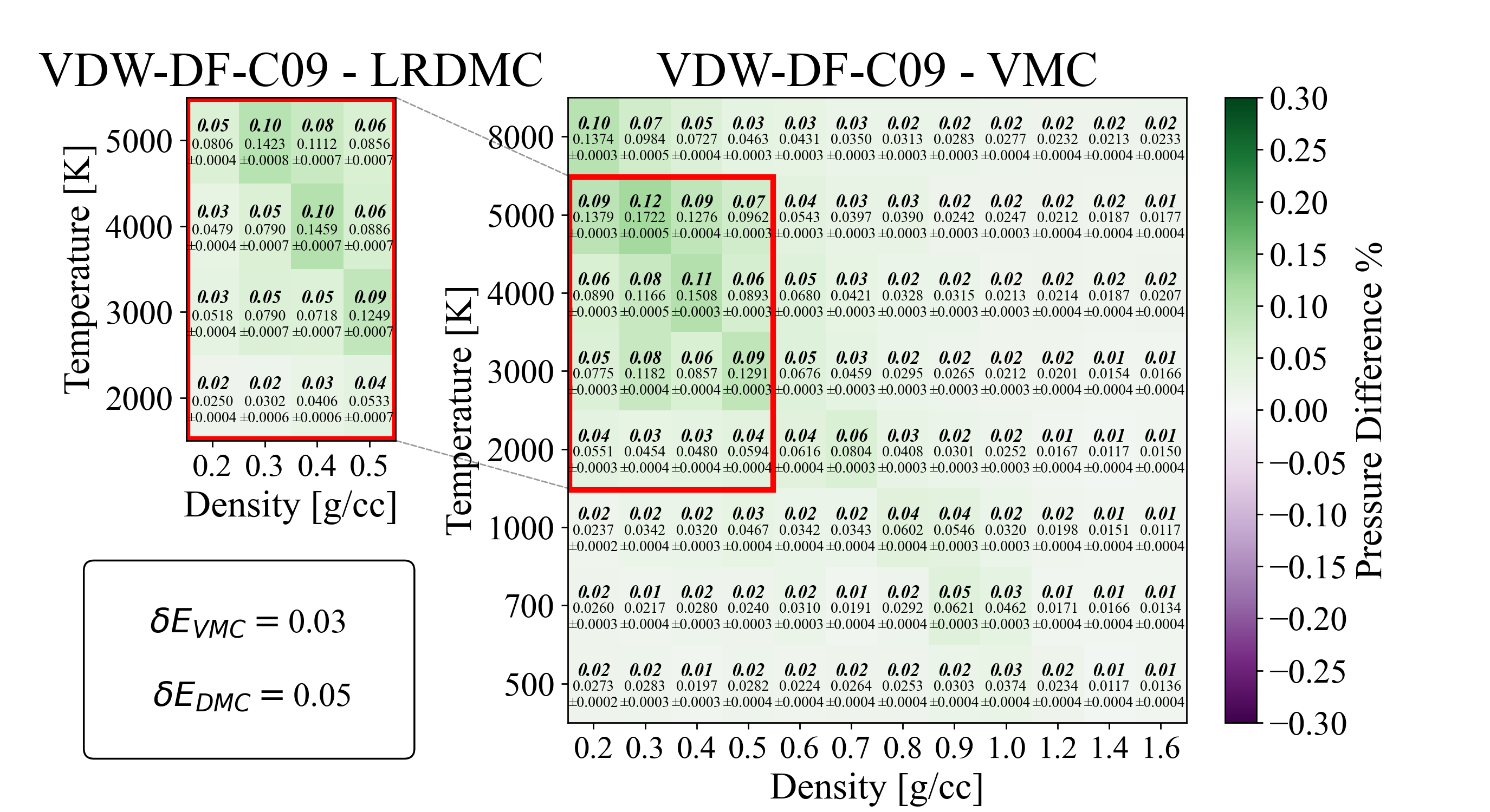
(g)

(h)

Figure 15: Part 1. Internal Energy benchmark of the DFT xc functional against VMC and LRDMC for the $T-\rho$ of interest. In every cell the bold value is the relative difference, while the lower value is the absolute difference with error. These values are computed as in Eq.9. The values in the box of every image are computed as Eq.10, exchanging $E$ with $P$ .

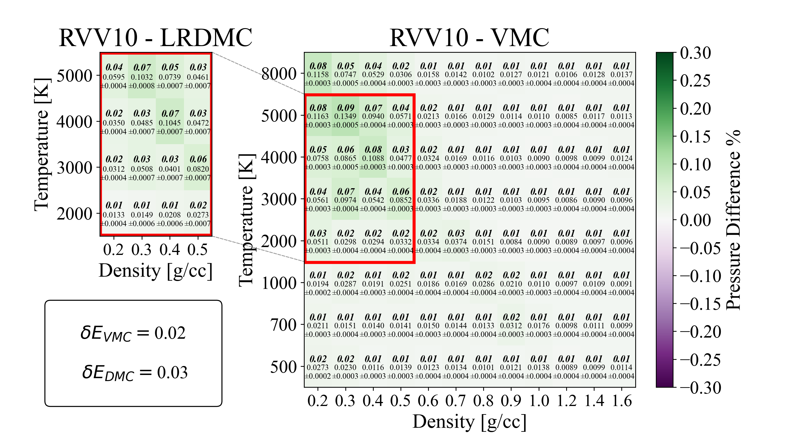
(a)

(b)

(c)

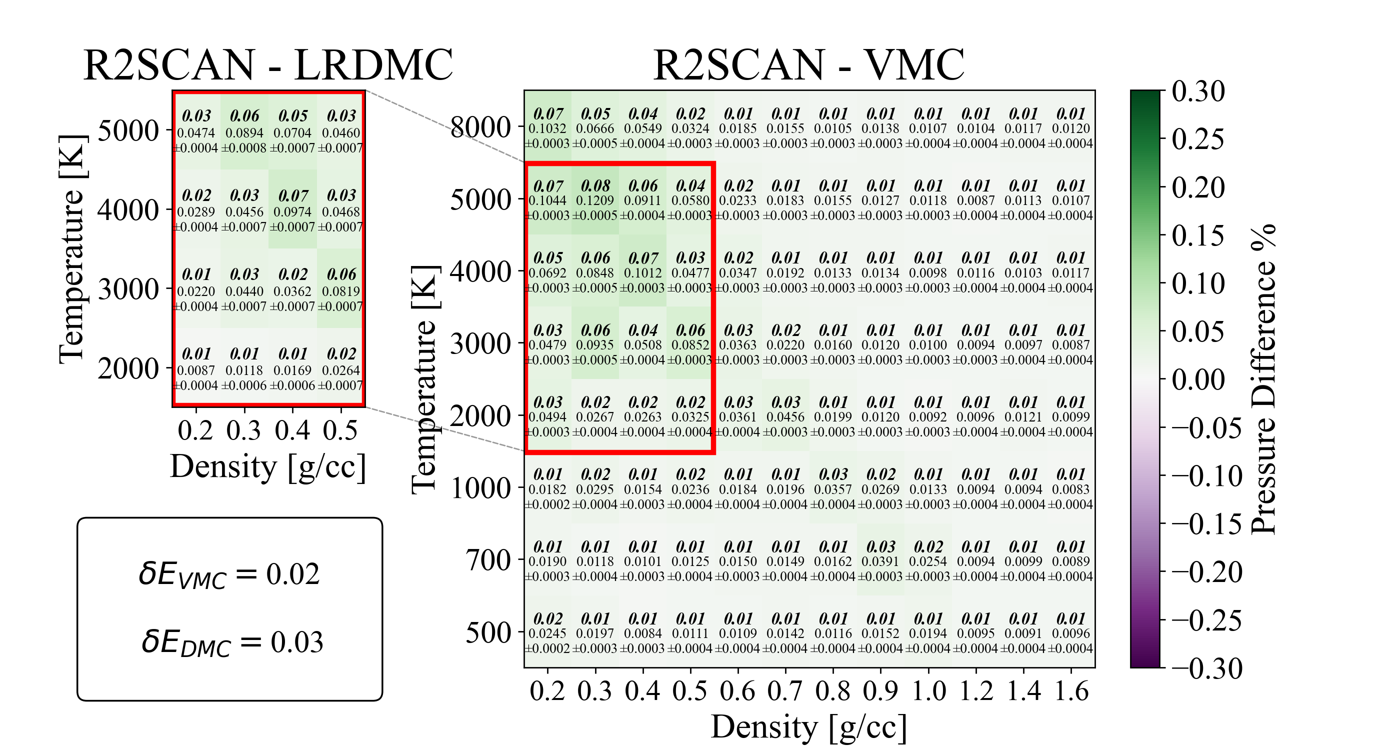
(d)

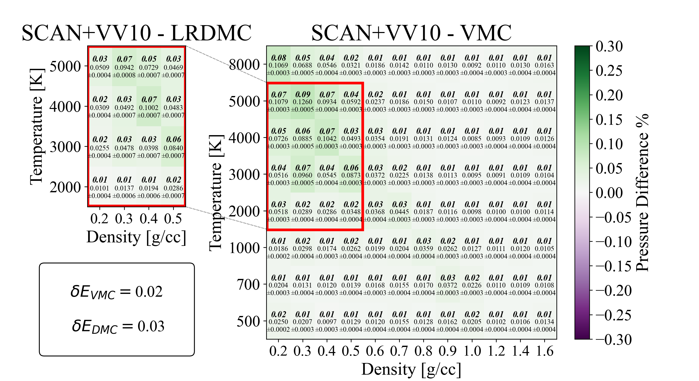
(e)

(f)

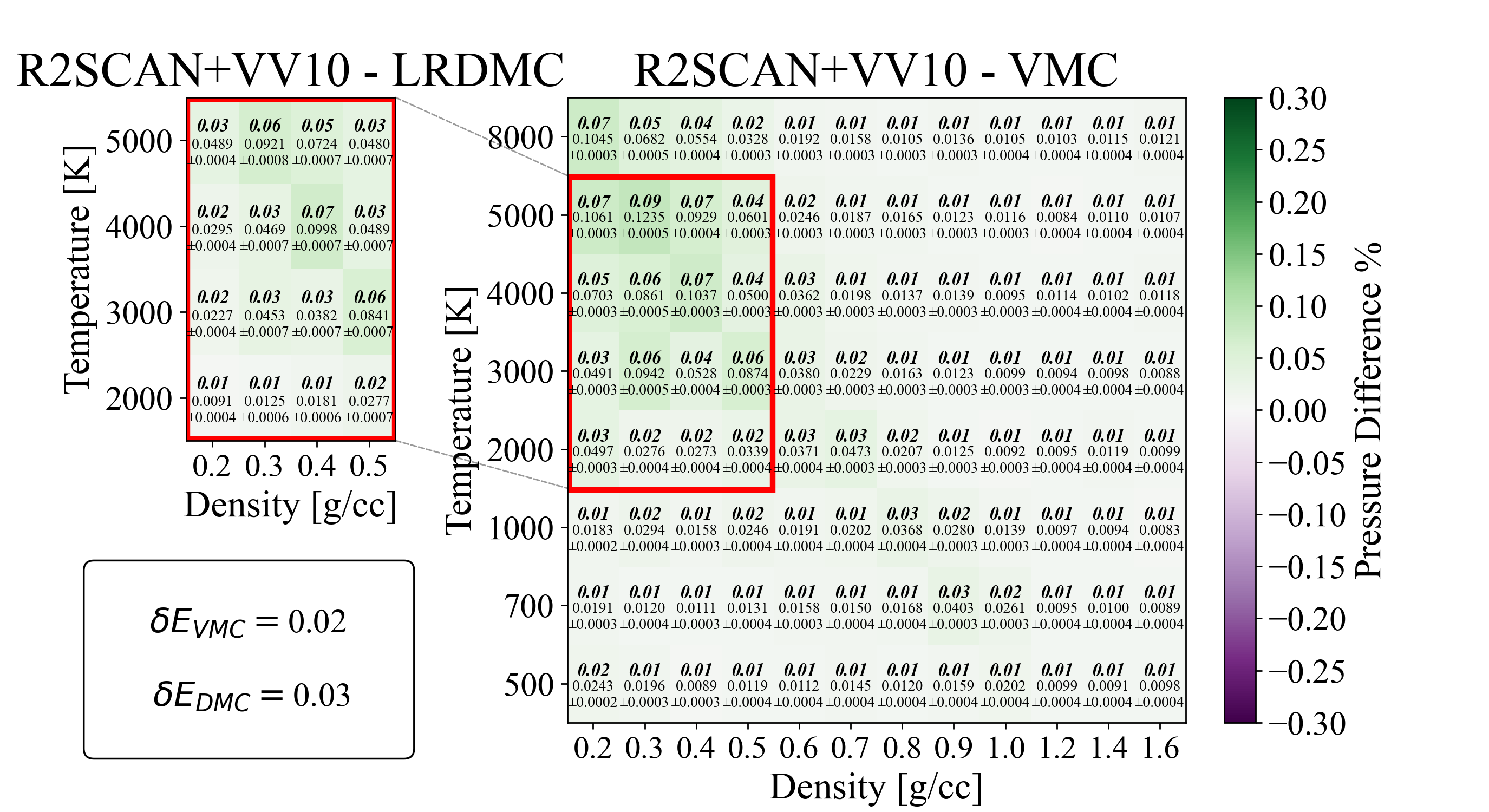
(g)

Figure 16: Part 2. Internal Energy benchmark of the DFT xc functional against VMC and LRDMC for the $T-\rho$ of interest. In every cell the bold value is the relative difference, while the lower value is the absolute difference with error. These values are computed as in Eq.9. The values in the box of every image are computed as Eq.10, exchanging $E$ with $P$.

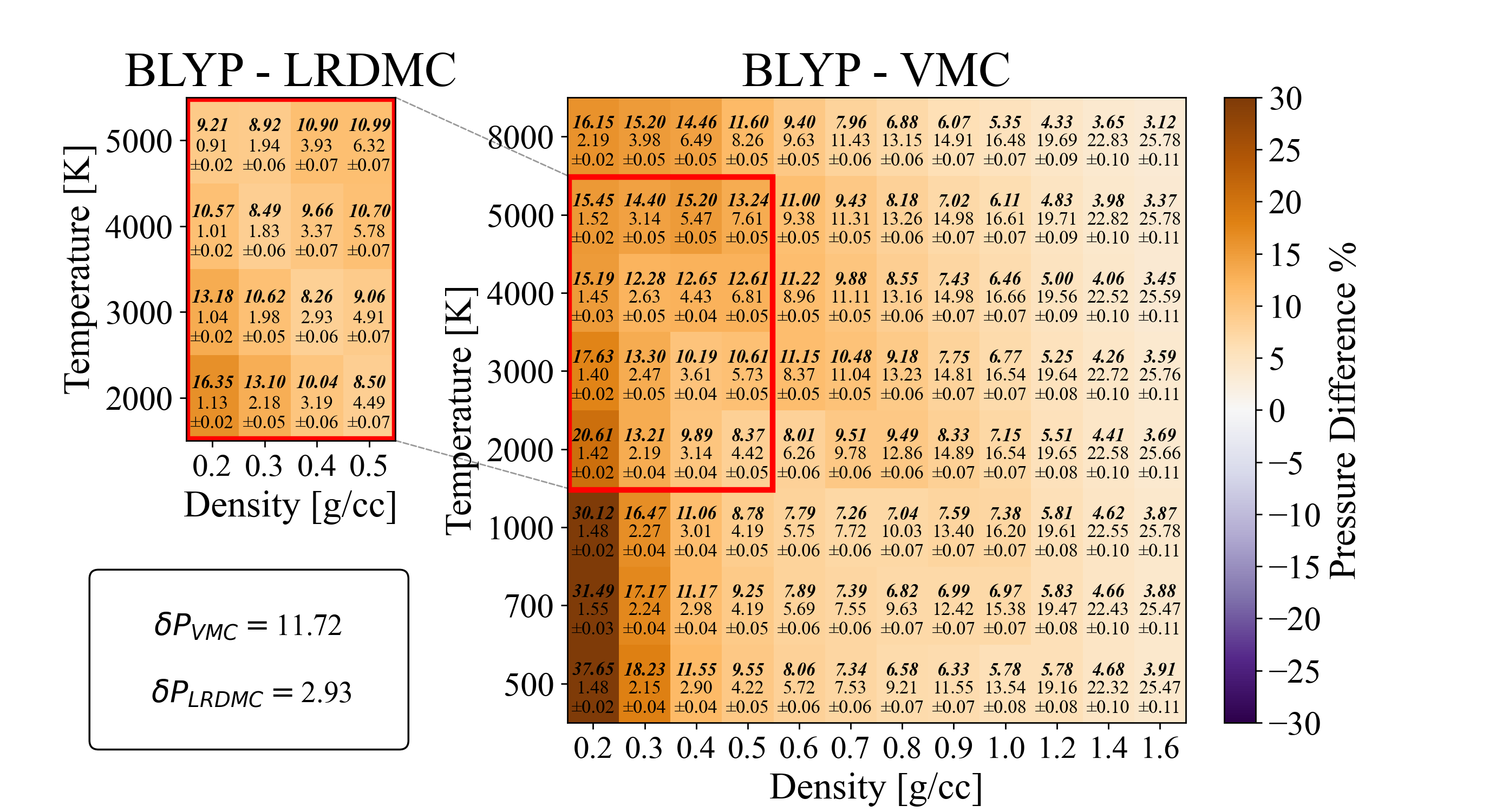
(a)

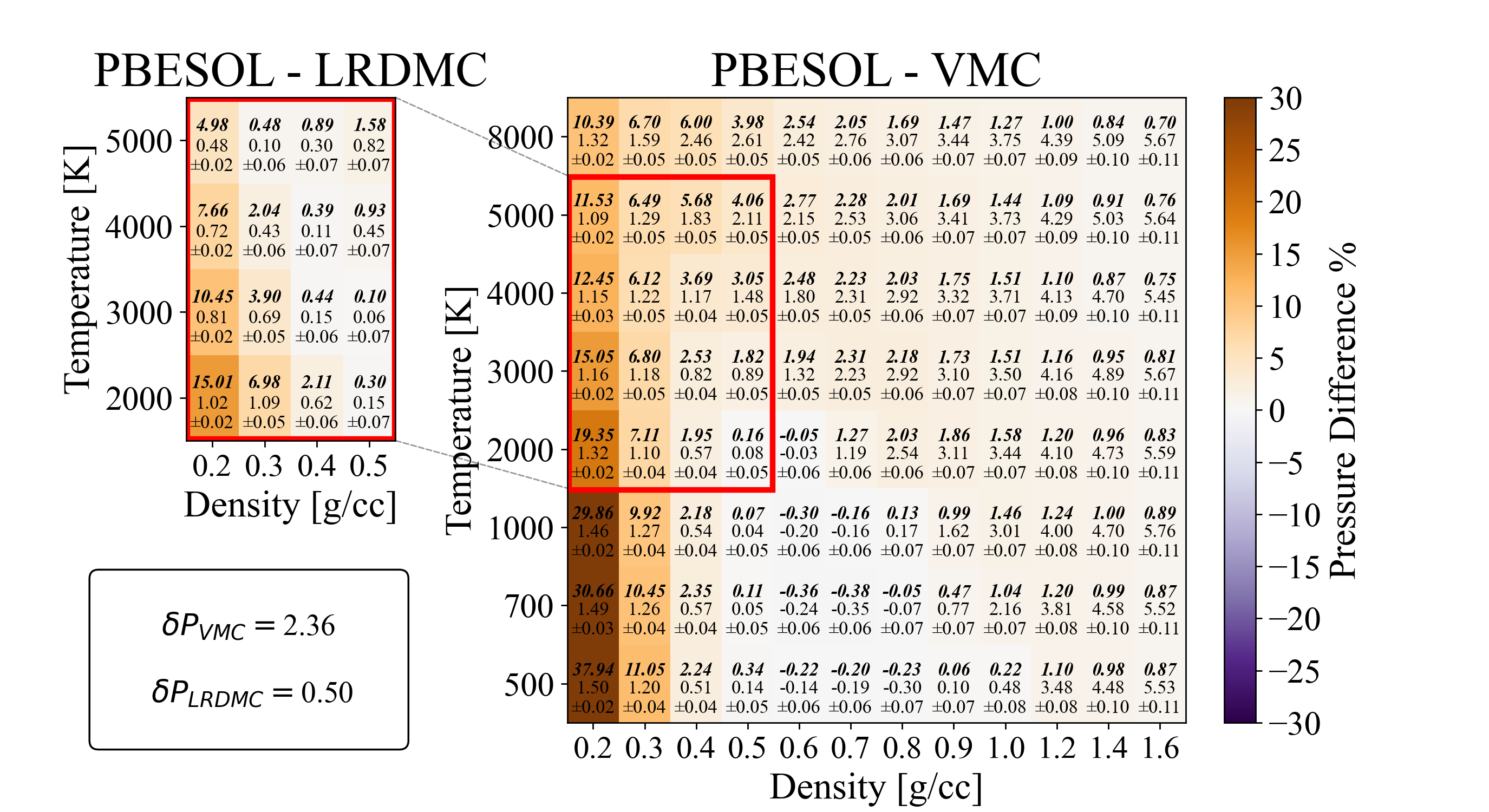
(b)

(c)

(d)

(e)

(f)

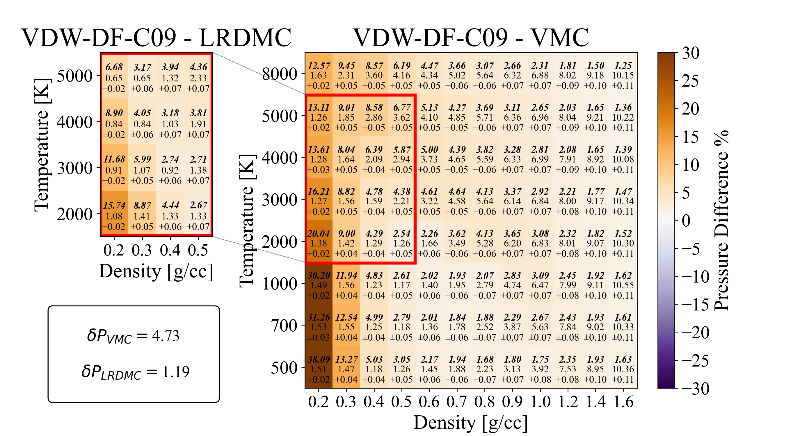
(g)

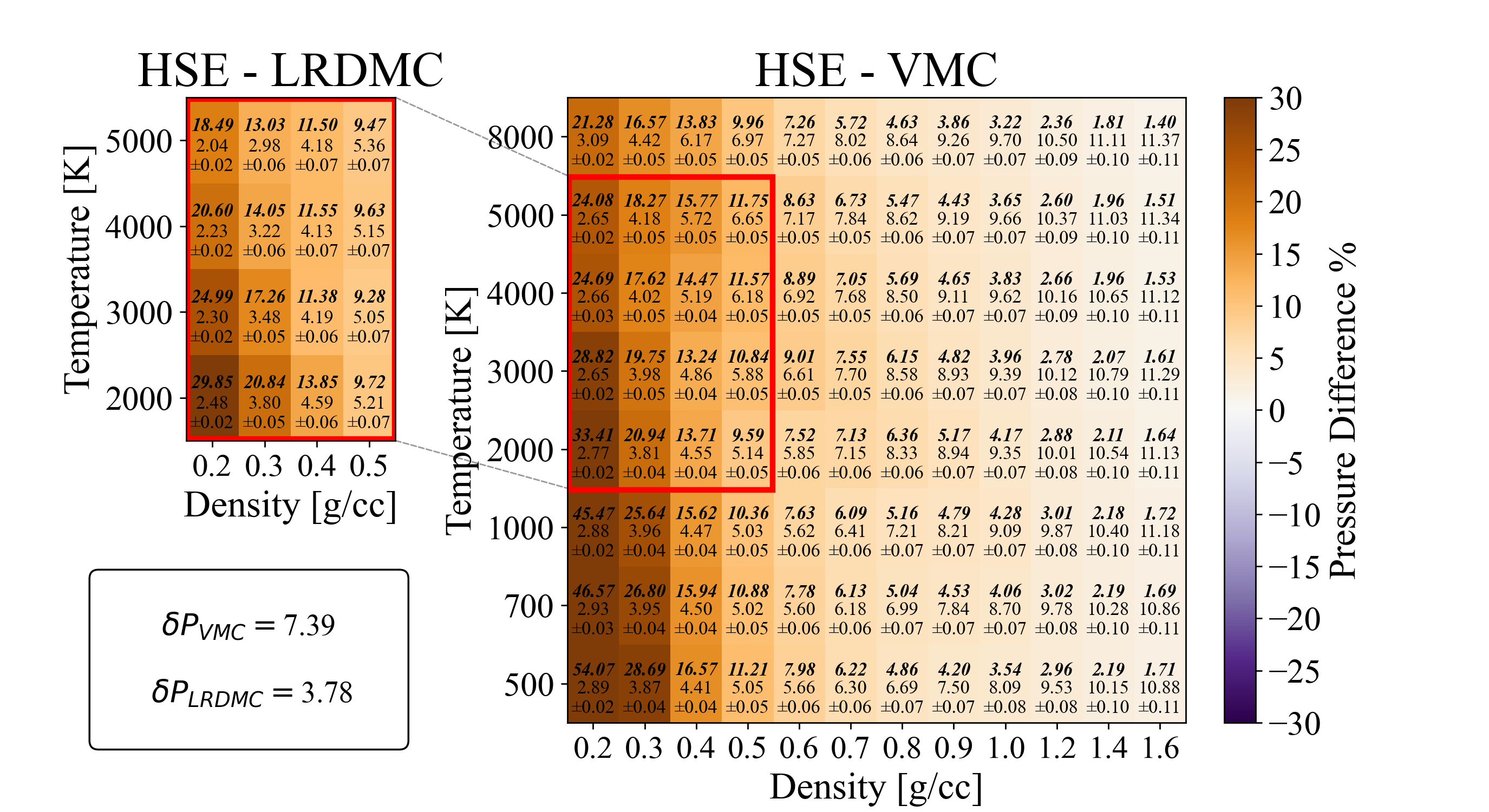
(h)

Figure 17: Part 1. Pressure benchmark of the DFT xc functional against VMC and LRDMC for the $T-\rho$ of interest. In every cell the bold value is the relative difference, while the lower value is the absolute difference with error. These values are computed as in Eq.8. The values in the box of every image are computed as Eq.10.

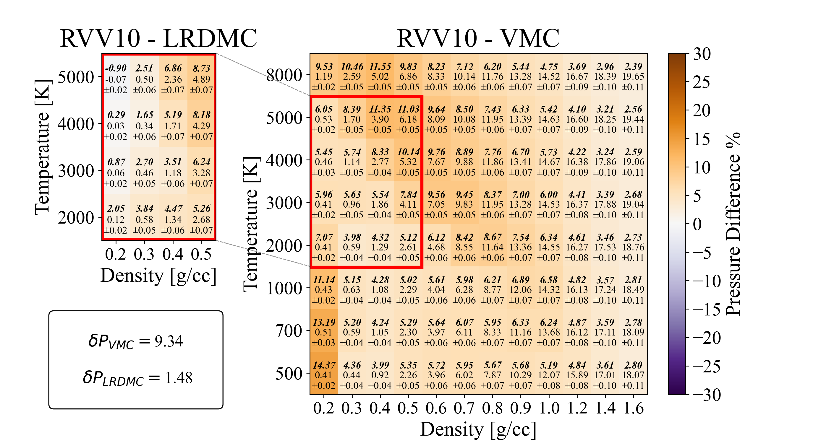
(a)

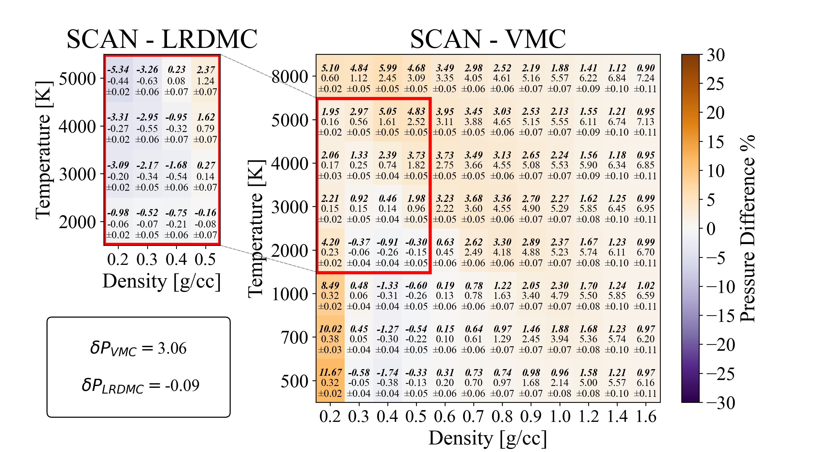
(b)

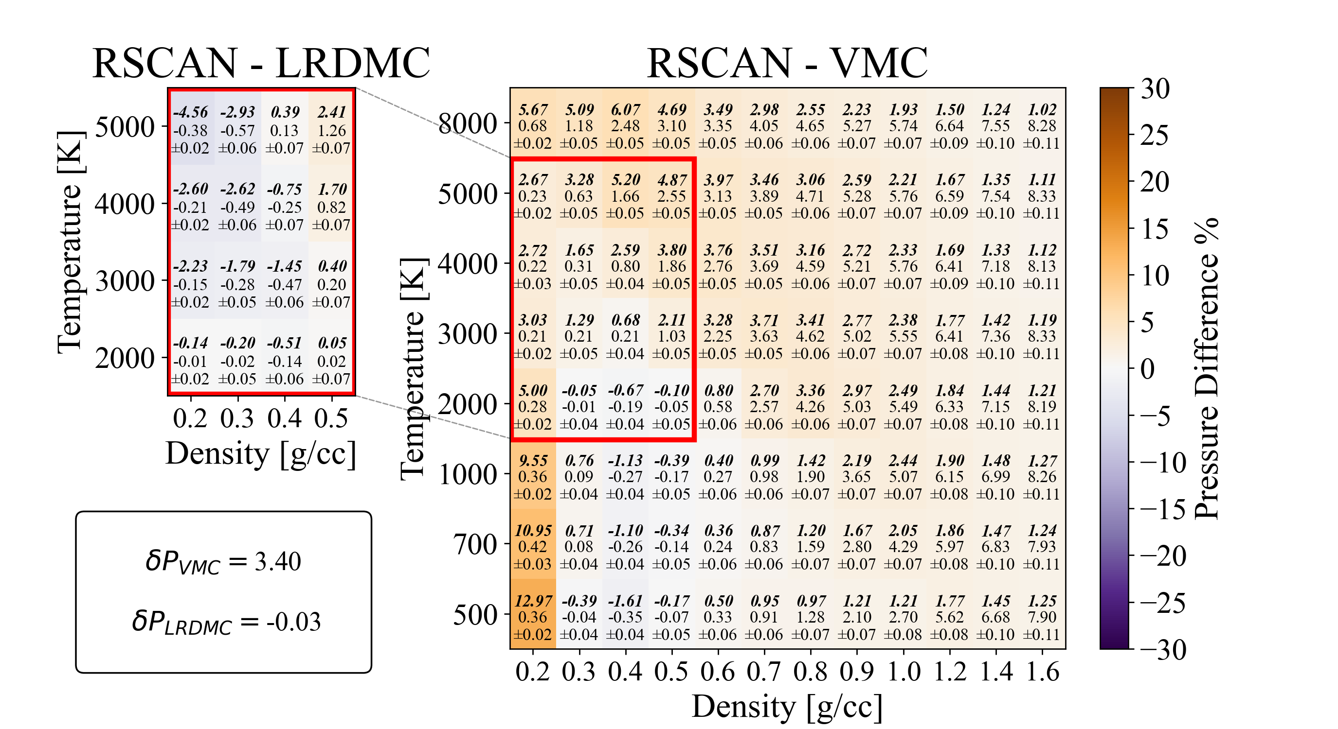
(c)

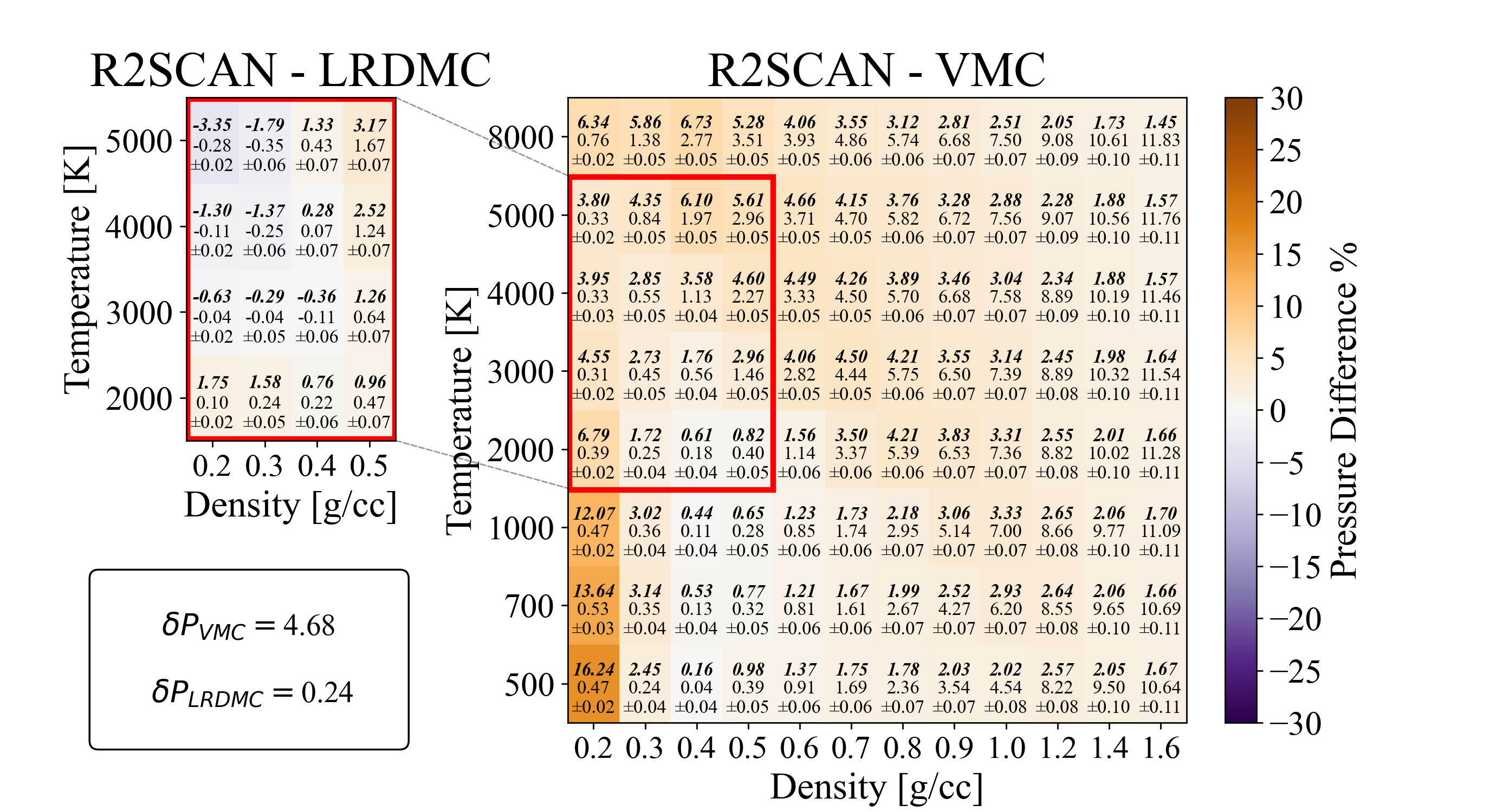
(d)

(e)

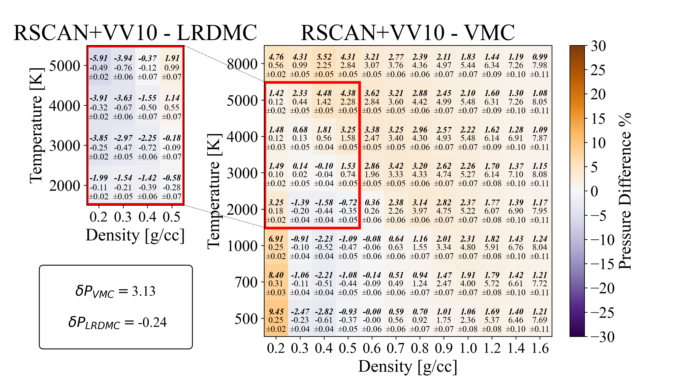
(f)

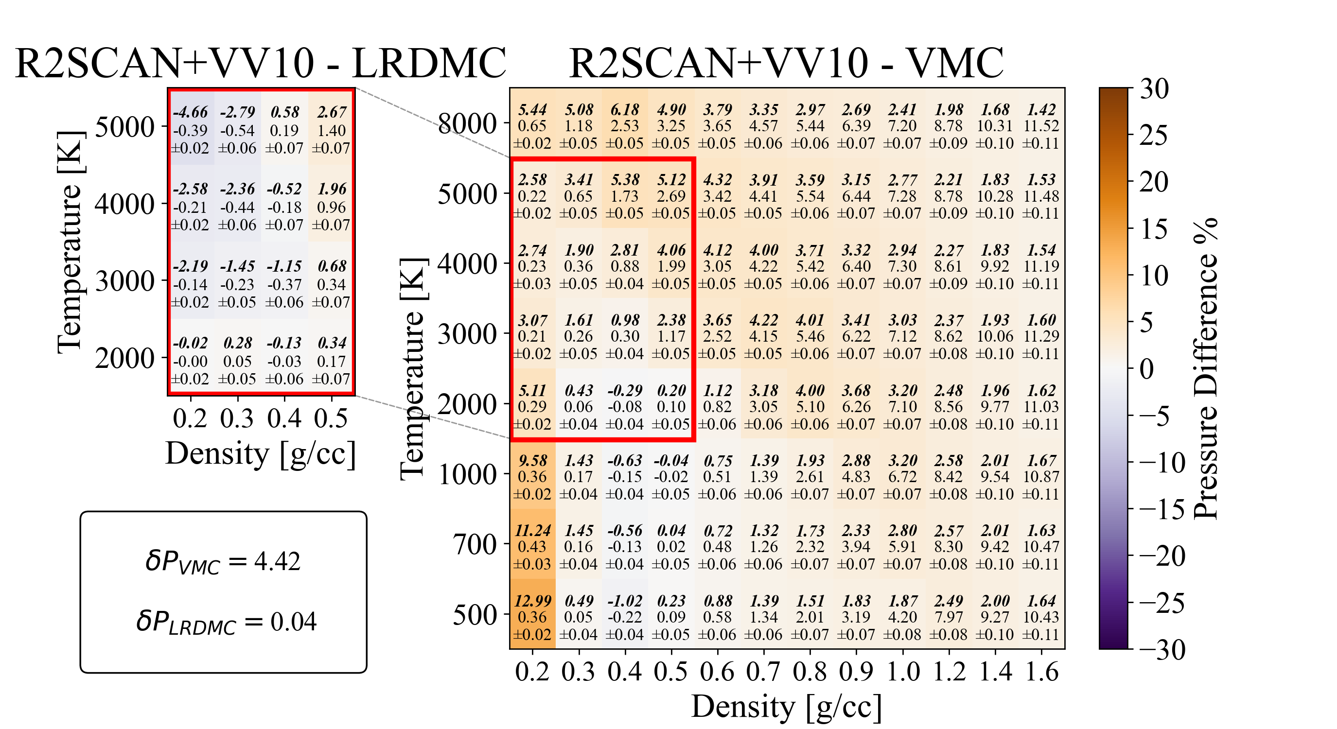
(g)

Figure 18: Part 2. Pressure benchmark of the DFT xc functional against VMC and LRDMC for the $T-\rho$ of interest. In every cell the bold value is the relative difference, while the lower value is the absolute difference with error. These values are computed as in Eq.8. The values in the box of every image are computed as Eq.10.

References

- McMahon et al. [2012] J. M. McMahon, M. A. Morales, C. Pierleoni, and D. M. Ceperley, The properties of hydrogen and helium under extreme conditions, Reviews of Modern Physics 84, 1607 (2012).
- Helled et al. [2020] R. Helled, G. Mazzola, and R. Redmer, Understanding dense hydrogen at planetary conditions, Nature Reviews Physics 2, 562 (2020).
- Wigner and Huntington [1935] E. Wigner and H. B. Huntington, On the possibility of a metallic modification of hydrogen, The Journal of Chemical Physics 3, 764 (1935).
- Ginzburg [2004] V. L. Ginzburg, Nobel lecture: On superconductivity and superfluidity (what i have and have not managed to do) as well as on the “physical minimum” at the beginning of the xxi century, Rev. Mod. Phys. 76, 981 (2004).
- Dalladay-Simpson et al. [2016] P. Dalladay-Simpson, R. T. Howie, and E. Gregoryanz, Evidence for a new phase of dense hydrogen above 325 gigapascals, Nature 529, 63 (2016).
- Dias and Silvera [2017] R. P. Dias and I. F. Silvera, Observation of the wigner-huntington transition to metallic hydrogen, Science 10.1126/science.aal1579 (2017).
- Loubeyre et al. [2020] P. Loubeyre, F. Occelli, and P. Dumas, Synchrotron infrared spectroscopic evidence of the probable transition to metal hydrogen, Nature 577, 631 (2020).
- Weir et al. [1996] S. Weir, A. Mitchell, and W. Nellis, Metallization of fluid molecular hydrogen at 140 gpa (1.4 mbar), Physical Review Letters 76, 1860 (1996).
- Celliers et al. [2018] P. M. Celliers, M. Millot, S. Brygoo, R. S. McWilliams, D. E. Fratanduono, J. R. Rygg, A. F. Goncharov, P. Loubeyre, J. H. Eggert, J. L. Peterson, N. B. Meezan, S. Le Pape, G. W. Collins, R. Jeanloz, and R. J. Hemley, Insulator-metal transition in dense fluid deuterium, Science 361, 677 (2018).
- Knudson et al. [2015] M. Knudson, M. Desjarlais, A. Becker, R. Lemke, K. Cochrane, M. Savage, D. Bliss, T. Mattsson, and R. Redmer, Direct observation of an abrupt insulator-to-metal transition in dense liquid deuterium, Science 348, 1455 (2015).
- Lühr et al. [2018] H. Lühr, J. Wicht, S. A. Gilder, and M. Holschneider, Magnetic Fields in the Solar System, Vol. 448 (Springer, 2018).
- Durante et al. [2020] D. Durante, M. Parisi, D. Serra, M. Zannoni, V. Notaro, P. Racioppa, D. R. Buccino, G. Lari, L. Gomez Casajus, L. Iess, W. M. Folkner, G. Tommei, P. Tortora, and S. J. Bolton, Jupiter’s Gravity Field Halfway Through the Juno Mission, Geophysical Research Letter 47, e86572 (2020).
- Iess et al. [2019] L. Iess, B. Militzer, Y. Kaspi, P. Nicholson, D. Durante, P. Racioppa, A. Anabtawi, E. Galanti, W. Hubbard, M. J. Mariani, P. Tortora, S. Wahl, and M. Zannoni, Measurement and implications of Saturn’s gravity field and ring mass, Science 364, aat2965 (2019).
- Helled and Howard [2024] R. Helled and S. Howard, Giant planet interiors and atmospheres, arXiv e-prints , arXiv:2407.05853 (2024), arXiv:2407.05853 [astro-ph.EP] .
- Miguel et al. [2016] Y. Miguel, T. Guillot, and L. Fayon, Jupiter internal structure: the effect of different equations of state, A&A 596, A114 (2016).
- Howard et al. [2023a] S. Howard, T. Guillot, M. Bazot, Y. Miguel, D. J. Stevenson, E. Galanti, Y. Kaspi, W. B. Hubbard, B. Militzer, R. Helled, N. Nettelmann, B. Idini, and S. Bolton, Jupiter’s interior from Juno: Equation-of-state uncertainties and dilute core extent, Astronomy and Astrophysics 672, A33 (2023a), arXiv:2302.09082 [astro-ph.EP] .
- Miguel et al. [2022] Y. Miguel, M. Bazot, T. Guillot, S. Howard, E. Galanti, Y. Kaspi, W. B. Hubbard, B. Militzer, R. Helled, S. K. Atreya, J. E. P. Connerney, D. Durante, L. Kulowski, J. I. Lunine, D. Stevenson, and S. Bolton, Jupiter’s inhomogeneous envelope, Astronomy & Astrophysics 662, A18 (2022), arXiv:2203.01866 [astro-ph.EP] .
- Wahl [2017] S. e. a. Wahl, Comparing Jupiter interior structure models to Juno gravity measurements and the role of a dilute core, Geophys. Res. Lett. 44, 80 (2017).
- Nettelmann et al. [2021] N. Nettelmann, N. Movshovitz, D. Ni, J. J. Fortney, E. Galanti, Y. Kaspi, R. Helled, C. R. Mankovich, and S. Bolton, Theory of Figures to the Seventh Order and the Interiors of Jupiter and Saturn, The Planetary Science Journal 2, 241 (2021), arXiv:2110.15452 [astro-ph.EP] .
- Militzer et al. [2022] B. Militzer, W. B. Hubbard, S. Wahl, J. I. Lunine, E. Galanti, Y. Kaspi, Y. Miguel, T. Guillot, K. M. Moore, M. Parisi, J. E. P. Connerney, R. Helled, H. Cao, C. Mankovich, D. J. Stevenson, R. S. Park, M. Wong, S. K. Atreya, J. Anderson, and S. J. Bolton, Juno Spacecraft Measurements of Jupiter’s Gravity Imply a Dilute Core, The Planetary Science Journal 3, 185 (2022).
- Stevenson [2020] D. J. Stevenson, Jupiter’s Interior as Revealed by Juno, Annual Review of Earth and Planetary Sciences 48, 465 (2020).
- Saumon et al. [1995] D. Saumon, G. Chabrier, and H. M. van Horn, An equation of state for low-mass stars and giant planets, Astrophysical Journal Supplement v. 99, p. 713 99, 713 (1995).
- Nettelmann et al. [2012] N. Nettelmann, A. Becker, B. Holst, and R. Redmer, Jupiter models with improved ab initio hydrogen equation of state (h-reos.2), The Astrophysical Journal 750, 52 (2012).
- Militzer and Hubbard [2013] B. Militzer and W. B. Hubbard, Ab initio equation of state for hydrogen-helium mixtures with recalibration of the giant-planet mass-radius relation, The Astrophysical Journal 774, 148 (2013).
- Miguel, Y. et al. [2018] Miguel, Y., Guillot, T., and Fayon, L., Jupiter internal structure: the effect of different equations of state (corrigendum), A&A 618, C2 (2018).
- Xie et al. [2025] H. Xie, S. Howard, and G. Mazzola, Accurate and thermodynamically consistent hydrogen equation of state for planetary modeling with flow matching (2025), arXiv:2501.10594 [astro-ph.EP] .
- Chabrier et al. [2019] G. Chabrier, S. Mazevet, and F. Soubiran, A new equation of state for dense hydrogen–helium mixtures, The Astrophysical Journal 872, 51 (2019).
- Becker et al. [2014] A. Becker, W. Lorenzen, J. J. Fortney, N. Nettelmann, M. Schöttler, and R. Redmer, Ab initio equations of state for hydrogen (h-reos. 3) and helium (he-reos. 3) and their implications for the interior of brown dwarfs, The Astrophysical Journal Supplement Series 215, 21 (2014).
- Burke [2012] K. Burke, Perspective on density functional theory, The Journal of Chemical Physics 136, 150901 (2012).
- Azadi and Foulkes [2013] S. Azadi and W. M. C. Foulkes, Fate of density functional theory in the study of high-pressure solid hydrogen, Physical Review B 88, 014115 (2013).
- Mazzola et al. [2018] G. Mazzola, R. Helled, and S. Sorella, Phase diagram of hydrogen and a hydrogen-helium mixture at planetary conditions by quantum monte carlo simulations, Phys. Rev. Lett. 120, 025701 (2018).
- Pierleoni et al. [2016] C. Pierleoni, M. A. Morales, G. Rillo, M. Holzmann, and D. M. Ceperley, Liquid–liquid phase transition in hydrogen by coupled electron–ion monte carlo simulations, Proceedings of the National Academy of Sciences 113, 4953 (2016).
- Bonitz et al. [2024] M. Bonitz, J. Vorberger, M. Bethkenhagen, M. P. Böhme, D. M. Ceperley, A. Filinov, T. Gawne, F. Graziani, G. Gregori, P. Hamann, S. B. Hansen, M. Holzmann, S. X. Hu, H. Kählert, V. V. Karasiev, U. Kleinschmidt, L. Kordts, C. Makait, B. Militzer, Z. A. Moldabekov, C. Pierleoni, M. Preising, K. Ramakrishna, R. Redmer, S. Schwalbe, P. Svensson, and T. Dornheim, Toward first principles-based simulations of dense hydrogen, Physics of Plasmas 31, 10.1063/5.0219405 (2024).
- Martin et al. [2016] R. M. Martin, L. Reining, and D. M. Ceperley, Interacting electrons (Cambridge University Press, 2016).
- Marx and Hutter [2009] D. Marx and J. Hutter, Ab initio molecular dynamics: basic theory and advanced methods (Cambridge University Press, 2009).
- Van De Bund et al. [2021] S. Van De Bund, H. Wiebe, and G. J. Ackland, Isotope quantum effects in the metallization transition in liquid hydrogen, Physical Review Letters 126, 225701 (2021).
- Zaghoo et al. [2018] M. Zaghoo, R. J. Husband, and I. F. Silvera, Striking isotope effect on the metallization phase lines of liquid hydrogen and deuterium, Physical Review B 98, 104102 (2018).
- Schuch and Verstraete [2009] N. Schuch and F. Verstraete, Computational complexity of interacting electrons and fundamental limitations of density functional theory, Nature physics 5, 732 (2009).
- Lorenzen et al. [2010] W. Lorenzen, B. Holst, and R. Redmer, First-order liquid-liquid phase transition in dense hydrogen, Phys. Rev. B 82, 195107 (2010).
- Jones [2015] R. O. Jones, Density functional theory: Its origins, rise to prominence, and future, Rev. Mod. Phys. 87, 897 (2015).
- Lejaeghere et al. [2016] K. Lejaeghere, G. Bihlmayer, T. Björkman, P. Blaha, S. Blügel, V. Blum, D. Caliste, I. E. Castelli, S. J. Clark, A. Dal Corso, et al., Reproducibility in density functional theory calculations of solids, Science 351, aad3000 (2016).
- Bosoni et al. [2023] E. Bosoni, L. Beal, M. Bercx, P. Blaha, S. Blügel, J. Bröder, M. Callsen, S. Cottenier, A. Degomme, V. Dikan, K. Eimre, E. Flage-Larsen, M. Fornari, A. Garcia, L. Genovese, M. Giantomassi, S. P. Huber, H. Janssen, G. Kastlunger, M. Krack, G. Kresse, T. D. Kühne, K. Lejaeghere, G. K. H. Madsen, M. Marsman, N. Marzari, G. Michalicek, H. Mirhosseini, T. M. A. Müller, G. Petretto, C. J. Pickard, S. Poncé, G.-M. Rignanese, O. Rubel, T. Ruh, M. Sluydts, D. E. P. Vanpoucke, S. Vijay, M. Wolloch, D. Wortmann, A. V. Yakutovich, J. Yu, A. Zadoks, B. Zhu, and G. Pizzi, How to verify the precision of density-functional-theory implementations via reproducible and universal workflows, Nature Reviews Physics 6, 45–58 (2023).
- Hohenberg and Kohn [1964] P. Hohenberg and W. Kohn, Inhomogeneous electron gas, Phys. Rev. 136, B864 (1964).
- Kohn and Sham [1965] W. Kohn and L. J. Sham, Self-consistent equations including exchange and correlation effects, Phys. Rev. 140, A1133 (1965).
- Martin [2004] R. M. Martin, Electronic Structure: Basic Theory and Practical Methods (Cambridge University Press, 2004).
- Perdew et al. [1996a] J. P. Perdew, K. Burke, and M. Ernzerhof, Generalized gradient approximation made simple, Phys. Rev. Lett. 77, 3865 (1996a).
- Chabrier and Debras [2021] G. Chabrier and F. Debras, A new equation of state for dense hydrogen–helium mixtures. ii. taking into account hydrogen–helium interactions, The Astrophysical Journal 917, 4 (2021).
- Becke [1988] A. D. Becke, Density-functional exchange-energy approximation with correct asymptotic behavior, Physical review A 38, 3098 (1988).
- Lee et al. [1988] C. Lee, W. Yang, and R. G. Parr, Development of the colle-salvetti correlation-energy formula into a functional of the electron density, Physical review B 37, 785 (1988).
- Dion et al. [2004] M. Dion, H. Rydberg, E. Schröder, D. C. Langreth, and B. I. Lundqvist, Van der waals density functional for general geometries, Physical review letters 92, 246401 (2004).
- Thonhauser et al. [2015] T. Thonhauser, S. Zuluaga, C. Arter, K. Berland, E. Schröder, and P. Hyldgaard, Spin signature of nonlocal correlation binding in metal-organic frameworks, Physical review letters 115, 136402 (2015).
- Lee et al. [2010] K. Lee, É. D. Murray, L. Kong, B. I. Lundqvist, and D. C. Langreth, Higher-accuracy van der waals density functional, Physical Review B—Condensed Matter and Materials Physics 82, 081101 (2010).
- Sun et al. [2015] J. Sun, A. Ruzsinszky, and J. P. Perdew, Strongly constrained and appropriately normed semilocal density functional, Physical review letters 115, 036402 (2015).
- Clay et al. [2014] R. C. Clay, J. Mcminis, J. M. McMahon, C. Pierleoni, D. M. Ceperley, and M. A. Morales, Benchmarking exchange-correlation functionals for hydrogen at high pressures using quantum monte carlo, Phys. Rev. B 89, 184106 (2014).
- Yang et al. [2020] H.-C. Yang, K. Liu, Z.-Y. Lu, and H.-Q. Lin, First-principles study of solid hydrogen: Comparison among four exchange-correlation functionals, Phys. Rev. B 102, 174109 (2020).
- Schöttler and Redmer [2018] M. Schöttler and R. Redmer, Ab initio calculation of the miscibility diagram for hydrogen-helium mixtures, Phys. Rev. Lett. 120, 115703 (2018).
- Azadi and Ackland [2017] S. Azadi and G. J. Ackland, The role of van der waals and exchange interactions in high-pressure solid hydrogen, Physical Chemistry Chemical Physics 19, 21829 (2017).
- Lu et al. [2019] B. Lu, D. Kang, D. Wang, T. Gao, and J. Dai, Towards the same line of liquid–liquid phase transition of dense hydrogen from various theoretical predictions, Chinese Physics Letters 36, 103102 (2019).
- Hinz et al. [2020] J. Hinz, V. V. Karasiev, S. Hu, M. Zaghoo, D. Mejía-Rodríguez, S. Trickey, and L. Calderín, Fully consistent density functional theory determination of the insulator-metal transition boundary in warm dense hydrogen, Physical Review Research 2, 032065 (2020).
- Zaghoo et al. [2016] M. Zaghoo, A. Salamat, and I. F. Silvera, Evidence of a first-order phase transition to metallic hydrogen, Physical Review B 93, 155128 (2016).
- Zaghoo and Silvera [2017] M. Zaghoo and I. F. Silvera, Conductivity and dissociation in liquid metallic hydrogen and implications for planetary interiors, Proceedings of the National Academy of Sciences 114, 11873 (2017).
- Ji et al. [2019] C. Ji, B. Li, W. Liu, J. S. Smith, A. Majumdar, W. Luo, R. Ahuja, J. Shu, J. Wang, S. Sinogeikin, et al., Ultrahigh-pressure isostructural electronic transitions in hydrogen, Nature 573, 558 (2019).
- Morales et al. [2013] M. A. Morales, J. M. McMahon, C. Pierleoni, and D. M. Ceperley, Nuclear quantum effects and nonlocal exchange-correlation functionals applied to liquid hydrogen at high pressure, Physical Review Letters 110, 065702 (2013).
- Geng et al. [2019] H. Y. Geng, Q. Wu, M. Marqués, and G. J. Ackland, Thermodynamic anomalies and three distinct liquid-liquid transitions in warm dense liquid hydrogen, Phys. Rev. B 100, 134109 (2019).
- Clay III et al. [2016] R. C. Clay III, M. Holzmann, D. M. Ceperley, and M. A. Morales, Benchmarking density functionals for hydrogen-helium mixtures with quantum monte carlo: Energetics, pressures, and forces, Physical Review B 93, 035121 (2016).
- Cohen et al. [2011] A. J. Cohen, P. Mori-Sánchez, and W. Yang, Challenges for density functional theory, Chemical Reviews 112, 289 (2011).
- Wagner et al. [2012] L. O. Wagner, E. Stoudenmire, K. Burke, and S. R. White, Reference electronic structure calculations in one dimension, Physical Chemistry Chemical Physics 14, 8581 (2012).
- Motta et al. [2017] M. Motta, D. M. Ceperley, G. K.-L. Chan, J. A. Gomez, E. Gull, S. Guo, C. A. Jiménez-Hoyos, T. N. Lan, J. Li, F. Ma, A. J. Millis, N. V. Prokof’ev, U. Ray, G. E. Scuseria, S. Sorella, E. M. Stoudenmire, Q. Sun, I. S. Tupitsyn, S. R. White, D. Zgid, and S. Zhang (Simons Collaboration on the Many-Electron Problem), Towards the solution of the many-electron problem in real materials: Equation of state of the hydrogen chain with state-of-the-art many-body methods, Phys. Rev. X 7, 031059 (2017).
- Dubeckyy et al. [2016] M. Dubeckyy, L. Mitas, and P. Jurecka, Noncovalent interactions by quantum monte carlo, Chemical reviews 116, 5188 (2016).
- Gillan et al. [2016] M. J. Gillan, D. Alfè, and A. Michaelides, Perspective: How good is dft for water?, The Journal of Chemical Physics 144, 130901 (2016).
- Foulkes et al. [2001] W. M. C. Foulkes, L. Mitas, R. J. Needs, and G. Rajagopal, Quantum monte carlo simulations of solids, Reviews of Modern Physics 73, 33 (2001).
- Nakano et al. [2020] K. Nakano, C. Attaccalite, M. Barborini, L. Capriotti, M. Casula, E. Coccia, M. Dagrada, C. Genovese, Y. Luo, G. Mazzola, A. Zen, and S. Sorella, Turborvb: A many-body toolkit for ab initio electronic simulations by quantum monte carlo, J. Chem. Phys. 152, 204121 (2020).
- Szabo and Ostlund [2012] A. Szabo and N. S. Ostlund, Modern quantum chemistry: introduction to advanced electronic structure theory (Courier Corporation, 2012).
- Riley et al. [2010] K. E. Riley, M. Pitonak, P. Jurecka, and P. Hobza, Stabilization and structure calculations for noncovalent interactions in extended molecular systems based on wave function and density functional theories, Chemical Reviews 110, 5023 (2010), pMID: 20486691, http://dx.doi.org/10.1021/cr1000173 .
- Casula et al. [2005] M. Casula, C. Filippi, and S. Sorella, Diffusion Monte Carlo method with lattice regularization, Phys. Rev. Lett. 95, 1 (2005).
- Nakano et al. [2023] K. Nakano, O. Kohulák, A. Raghav, M. Casula, and S. Sorella, TurboGenius: Python suite for high-throughput calculations of ab initio quantum Monte Carlo methods, J. Chem. Phys. 159, 224801 (2023).
- Mazzola et al. [2012] G. Mazzola, A. Zen, and S. Sorella, Finite-temperature electronic simulations without the born-oppenheimer constraint, The Journal of Chemical Physics 137, 134112 (2012).
- Hermann et al. [2020] J. Hermann, Z. Schätzle, and F. Noé, Deep-neural-network solution of the electronic schrödinger equation, Nature Chemistry 12, 891–897 (2020).
- Pescia et al. [2024] G. Pescia, J. Nys, J. Kim, A. Lovato, and G. Carleo, Message-passing neural quantum states for the homogeneous electron gas, Phys. Rev. B 110, 035108 (2024).
- Pfau et al. [2020] D. Pfau, J. S. Spencer, A. G. D. G. Matthews, and W. M. C. Foulkes, Ab initio solution of the many-electron schrödinger equation with deep neural networks, Phys. Rev. Res. 2, 033429 (2020).
- Sorella [1998] S. Sorella, Green function monte carlo with stochastic reconfiguration, Phys. Rev. Lett. 80, 4558 (1998).
- Sorella et al. [2007] S. Sorella, M. Casula, and D. Rocca, Weak binding between two aromatic rings: Feeling the van der waals attraction by quantum monte carlo methods, J. Chem. Phys. 127, 014105 (2007).
- Monacelli et al. [2023] L. Monacelli, M. Casula, K. Nakano, S. Sorella, and F. Mauri, Quantum phase diagram of high-pressure hydrogen, Nat. Phys. 19, 845 (2023).
- Raghav et al. [2023] A. Raghav, R. Maezono, K. Hongo, S. Sorella, and K. Nakano, Toward chemical accuracy using the jastrow correlated antisymmetrized geminal power ansatz, J. Chem. Theory Comput. 19, 2222 (2023).
- Becca and Sorella [2017] F. Becca and S. Sorella, Quantum Monte Carlo Approaches for Correlated Systems, 1st ed. (Cambridge University Press, 2017).
- Mazzola et al. [2014] G. Mazzola, S. Yunoki, and S. Sorella, Unexpectedly high pressure for molecular dissociation in liquid hydrogen by electronic simulation, Nature Communications 5, 3487 (2014).
- Zen et al. [2015] A. Zen, Y. Luo, G. Mazzola, L. Guidoni, and S. Sorella, Ab initio molecular dynamics simulation of liquid water by quantum monte carlo, The Journal of chemical physics 142, 144111 (2015).
- Cheng et al. [2020] B. Cheng, G. Mazzola, C. J. Pickard, and M. Ceriotti, Evidence for supercritical behaviour of high-pressure liquid hydrogen, Nature 585, 217 (2020).
- Tirelli et al. [2022] A. Tirelli, G. Tenti, K. Nakano, and S. Sorella, High-pressure hydrogen by machine learning and quantum monte carlo, Physical Review B 106, L041105 (2022).
- Niu et al. [2023] H. Niu, Y. Yang, S. Jensen, M. Holzmann, C. Pierleoni, and D. M. Ceperley, Stable solid molecular hydrogen above 900 k from a machine-learned potential trained with diffusion quantum monte carlo, Phys. Rev. Lett. 130, 076102 (2023).
- Goswami et al. [2024] S. Goswami, S. Jensen, Y. Yang, M. Holzmann, C. Pierleoni, and D. M. Ceperley, High temperature melting of dense molecular hydrogen from machine-learning interatomic potentials trained on quantum monte carlo (2024), arXiv:2411.15665 [physics.chem-ph] .
- Nakano et al. [2024] K. Nakano, M. Casula, and G. Tenti, Efficient calculation of unbiased atomic forces in ab initio variational monte carlo, Physical Review B 109, 205151 (2024).
- Allen and Tildesley [2017] M. P. Allen and D. J. Tildesley, Computer simulation of liquids (Oxford university press, 2017).
- Perdew et al. [2008] J. P. Perdew, A. Ruzsinszky, G. I. Csonka, O. A. Vydrov, G. E. Scuseria, L. A. Constantin, X. Zhou, and K. Burke, Restoring the density-gradient expansion for exchange in solids and surfaces, Physical review letters 100, 136406 (2008).
- Peng et al. [2016] H. Peng, Z.-H. Yang, J. P. Perdew, and J. Sun, Versatile van der waals density functional based on a meta-generalized gradient approximation, Physical Review X 6, 041005 (2016).
- Csonka et al. [2009] G. I. Csonka, J. P. Perdew, A. Ruzsinszky, P. H. T. Philipsen, S. Lebègue, J. Paier, O. A. Vydrov, and J. G. Ángyán, Assessing the performance of recent density functionals for bulk solids, Phys. Rev. B 79, 155107 (2009).
- Bonev et al. [2004] S. Bonev, E. Schwegler, G. Galli, and T. Ogitsu, A quantum fluid of metallic hydrogen suggested by first-principles calculations, Nature 431, 669 (2004).
- Morales et al. [2010] M. A. Morales, C. Pierleoni, E. Schwegler, and D. M. Ceperley, Evidence for a first-order liquid-liquid transition in high-pressure hydrogen from ab initio simulations, Proceedings of the National Academy of Sciences 107, 12799 (2010).
- Scandolo [2003] S. Scandolo, Liquid–liquid phase transition in compressed hydrogen from first-principles simulations, Proceedings of the National Academy of Sciences 100, 3051 (2003).
- Tamblyn and Bonev [2010] I. Tamblyn and S. A. Bonev, Structure and phase boundaries of compressed liquid hydrogen, Physical review letters 104, 065702 (2010).
- Bergermann et al. [2024] A. Bergermann, L. Kleindienst, and R. Redmer, Nonmetal-to-metal transition in liquid hydrogen using density functional theory and the heyd–scuseria–ernzerhof exchange-correlation functional, The Journal of Chemical Physics 161 (2024).
- Azadi et al. [2017] S. Azadi, N. D. Drummond, and W. M. C. Foulkes, Nature of the metallization transition in solid hydrogen, Physical Review B 95, 035142 (2017).
- Tiihonen et al. [2021] J. Tiihonen, R. C. Clay III, and J. T. Krogel, Toward quantum monte carlo forces on heavier ions: Scaling properties, J. Chem. Phys. 154, 204111 (2021).
- Nakano et al. [2022] K. Nakano, A. Raghav, and S. Sorella, Space-warp coordinate transformation for efficient ionic force calculations in quantum monte carlo, J. Chem. Phys. 156, 034101 (2022).
- Perdew et al. [1996b] J. P. Perdew, M. Ernzerhof, and K. Burke, Rationale for mixing exact exchange with density functional approximations, The Journal of chemical physics 105, 9982 (1996b).
- Berland et al. [2017] K. Berland, Y. Jiao, J.-H. Lee, T. Rangel, J. B. Neaton, and P. Hyldgaard, Assessment of two hybrid van der waals density functionals for covalent and non-covalent binding of molecules, The Journal of Chemical Physics 146 (2017).
- Vydrov and Van Voorhis [2010] O. A. Vydrov and T. Van Voorhis, Nonlocal van der waals density functional: The simpler the better, The Journal of chemical physics 133 (2010).
- Sabatini et al. [2013] R. Sabatini, T. Gorni, and S. De Gironcoli, Nonlocal van der waals density functional made simple and efficient, Physical Review B—Condensed Matter and Materials Physics 87, 041108 (2013).
- Heyd et al. [2003] J. Heyd, G. E. Scuseria, and M. Ernzerhof, Hybrid functionals based on a screened coulomb potential, The Journal of chemical physics 118, 8207 (2003).
- Bartók and Yates [2019] A. P. Bartók and J. R. Yates, Regularized scan functional, The Journal of chemical physics 150 (2019).
- Furness et al. [2020] J. W. Furness, A. D. Kaplan, J. Ning, J. P. Perdew, and J. Sun, Accurate and numerically efficient r2scan meta-generalized gradient approximation, The journal of physical chemistry letters 11, 8208 (2020).
- Mankovich and Fuller [2021] C. R. Mankovich and J. Fuller, A diffuse core in Saturn revealed by ring seismology, Nature Astronomy 5, 1103 (2021), arXiv:2104.13385 [astro-ph.EP] .
- Van Setten et al. [2018] M. J. Van Setten, M. Giantomassi, E. Bousquet, M. J. Verstraete, D. R. Hamann, X. Gonze, and G.-M. Rignanese, The pseudodojo: Training and grading a 85 element optimized norm-conserving pseudopotential table, Computer Physics Communications 226, 39 (2018).
- Hubbard [1975] W. B. Hubbard, Gravitational field of a rotating planet with a polytropic index of unity, Astronomicheskii Zhurnal 18, 621 (1975).
- Guillot and Morel [1995] T. Guillot and P. Morel, CEPAM: a code for modeling the interiors of giant planets., Astronomy and Astrophysics Suppl. 109, 109 (1995).
- Helled et al. [2022] R. Helled, D. J. Stevenson, J. I. Lunine, S. J. Bolton, N. Nettelmann, S. Atreya, T. Guillot, B. Militzer, Y. Miguel, and W. B. Hubbard, Revelations on Jupiter’s formation, evolution and interior: Challenges from Juno results, Icarus 378, 114937 (2022), arXiv:2202.10041 [astro-ph.EP] .
- Debras and Chabrier [2019] F. Debras and G. Chabrier, New Models of Jupiter in the Context of Juno and Galileo, ApJ 872, 100 (2019).
- Howard et al. [2023b] S. Howard, T. Guillot, S. Markham, R. Helled, S. Müller, D. J. Stevenson, J. I. Lunine, Y. Miguel, and N. Nettelmann, Exploring the hypothesis of an inverted Z gradient inside Jupiter, Astronomy and Astrophysics 680, L2 (2023b), arXiv:2311.07646 [astro-ph.EP] .
- Müller and Helled [2024] S. Müller and R. Helled, Can Jupiter’s Atmospheric Metallicity Be Different from the Deep Interior?, Astrophys. J. 967, 7 (2024), arXiv:2403.16273 [astro-ph.EP] .
- Giannozzi et al. [2009] P. Giannozzi, S. Baroni, N. Bonini, M. Calandra, R. Car, C. Cavazzoni, D. Ceresoli, G. L. Chiarotti, M. Cococcioni, I. Dabo, et al., Quantum espresso: a modular and open-source software project for quantum simulations of materials, Journal of physics: Condensed matter 21, 395502 (2009).
- Blöchl [1994] P. E. Blöchl, Projector augmented-wave method, Phys. Rev. B 50, 17953 (1994).
- Dal Corso [2014] A. Dal Corso, Pseudopotentials periodic table: From h to pu, Computational Materials Science 95, 337 (2014).
- Hamann et al. [1979] D. R. Hamann, M. Schlüter, and C. Chiang, Norm-conserving pseudopotentials, Phys. Rev. Lett. 43, 1494 (1979).
- Hamann [2013] D. R. Hamann, Optimized norm-conserving vanderbilt pseudopotentials, Phys. Rev. B 88, 085117 (2013).
- Yao and Kanai [2017] Y. Yao and Y. Kanai, Plane-wave pseudopotential implementation and performance of scan meta-gga exchange-correlation functional for extended systems, The Journal of chemical physics 146 (2017).
- Bussi et al. [2007] G. Bussi, D. Donadio, and M. Parrinello, Canonical sampling through velocity rescaling, The Journal of chemical physics 126, 014101 (2007).
- Kresse and Hafner [1993] G. Kresse and J. Hafner, Ab initio molecular dynamics for liquid metals, Physical review B 47, 558 (1993).
- Casula and Sorella [2003] M. Casula and S. Sorella, Geminal wave functions with jastrow correlation: A first application to atoms, J. Chem. Phys. 119, 6500 (2003).
- Pritchard et al. [2019] B. P. Pritchard, D. Altarawy, B. T. Didier, T. D. Gibson, and T. L. Windus, A new basis set exchange: An open, up-to-date resource for the molecular sciences community, J. Chem. Inf. Model. 59, 4814 (2019).
- Tenti et al. [2024] G. Tenti, K. Nakano, A. Tirelli, S. Sorella, and M. Casula, Principal deuterium hugoniot via quantum monte carlo and -learning, Phys. Rev. B 110, L041107 (2024).
- Nakano et al. [2019] K. Nakano, R. Maezono, and S. Sorella, All-electron quantum monte carlo with jastrow single determinant ansatz: Application to the sodium dimer, J. Chem. Theory Comput. 15, 4044 (2019).
- Reynolds et al. [1986] P. Reynolds, R. Barnett, B. Hammond, R. Grimes, and W. Lester Jr, Quantum chemistry by quantum monte carlo: Beyond ground-state energy calculations, Int. J. Quantum Chem. 29, 589 (1986).
- Assaraf and Caffarel [2000] R. Assaraf and M. Caffarel, Computing forces with quantum monte carlo, J. Chem. Phys. 113, 4028 (2000).
- Filippi and Umrigar [2000] C. Filippi and C. J. Umrigar, Correlated sampling in quantum monte carlo: A route to forces, Phys. Rev. B 61, R16291 (2000).
- Chiesa et al. [2005] S. Chiesa, D. M. Ceperley, and S. Zhang, Accurate, efficient, and simple forces computed with quantum monte carlo methods, Phys. Rev. Lett. 94, 036404 (2005).
- Badinski and Needs [2008] A. Badinski and R. J. Needs, Total forces in the diffusion monte carlo method with nonlocal pseudopotentials, Phys. Rev. B 78, 035134 (2008).
- Assaraf et al. [2011] R. Assaraf, M. Caffarel, and A. C. Kollias, Chaotic versus nonchaotic stochastic dynamics in monte carlo simulations: A route for accurate energy differences in -body systems, Phys. Rev. Lett. 106, 150601 (2011).
- Moroni et al. [2014] S. Moroni, S. Saccani, and C. Filippi, Practical schemes for accurate forces in quantum monte carlo, J. Chem. Theory Comput. 10, 4823 (2014).
- Van Rhijn et al. [2021] J. Van Rhijn, C. Filippi, S. De Palo, and S. Moroni, Energy derivatives in real-space diffusion monte carlo, J. Chem. Theory Comput. 18, 118 (2021).
- Slootman et al. [2024] E. Slootman, I. Poltavsky, R. Shinde, J. Cocomello, S. Moroni, A. Tkatchenko, and C. Filippi, Accurate quantum monte carlo forces for machine-learned force fields: Ethanol as a benchmark, Journal of chemical theory and computation 20, 6020 (2024).