Set-point control and local stability for flat nonlinear systems using model-following control

Abstract

We consider the set-point control problem for nonlinear systems with flat output that are subject to perturbations. The nonlinear dynamics as well as the perturbations are locally Lipschitz. We apply the model-following control (MFC) approach which consists of a model control loop (MCL) for a feedforward generation and a process control loop (PCL) that compensates the perturbations using high-gain feedback. We analyse the resulting closed-loop system and discuss its relation to a standard flatness-based high-gain approach. In particular we analyse the estimated region of attraction provided by a quadratic Lyapunov function. A case study illustrates the approach and quantifies the region of attraction obtained for each control approach. Using the initial condition of the model control loop as tuning parameter for the MFC design, provides that a significantly larger region of attraction can be guaranteed compared to a conventional single-loop high-gain design.

1 Introduction

Model-following control (MFC), also referred to as model reference control, is a well-established control architecture consisting of a reference or model control loop (MCL) and the actual process control loop (PCL). A typical configuration of such structure is depicted in Figure 1. This variation of the classical two-degree-of-freedom control structure [11] has been applied and studied in many variations and control applications [7, 1, 19, 33, 16, 12, 4].

The MCL typically contains a linear model with a feedback controller that is often considered as imposing the desired behaviour on the control system. The PCL is designed towards disturbance rejection. However, since the reference control loop also provides a nominal control signal $u^{\star}$ and corresponding output $y^{\star}$ this control loop can also be considered as a feedforward control [33] and trajectory generator [20, 9, 22].

In many cases the MFC structure shows better robustness properties w.r.t. model uncertainties and disturbances compared to a single-loop feedback system, see e. g. [25]. Not least for this reason, a linear approximation of the nonlinear process is often used in the MCL in various control applications, e. g. a robotic manipulator [14, 16, 15], the low-frequency motions of the drilling vessel Wimpey Sealab [6], an electric heater [24], speed control of a permanent magnet synchronous motor [17] or boom cranes [23].

Using a state-space model in the MCL the model-state $\bm{x}^{\star}$ is available as reference trajectory. In [1, 19, 5] tracking of the reference state generated by a linear feedback system is studied using state-feedback in the PCL. The structure has been studied including a disturbance injection [20, 33]. In [3] an MFC structure with a combination of output and state feedback is developed. Compared to the standard MFC structure the combined feedback shows better performance and robustness w.r.t parameter uncertainties. These results are obtained considering some case studies but a systematic analysis is not provided.

This paper contributes to the analysis of the MFC structure using a nonlinear model in the MCL. Such approach has been investigated in several case studies [18, 4, 12, 2, 21, 30] and shows good performance and robustness properties. In [29, 30] a local model network to model the nonlinear process is used in the MCL. This feedforward control shows better performance than a comparable inversion-based approach. Some initial analysis of the potential benefits using a nonlinear model in the MCL is found in [31, 32, 28]. In [31] it is shown that the increase of robustness can be quantified in terms of the norm bound on the uncertainty. In [32] a high-gain control is applied to the PCL using feedback-linearisation based on the nominal nonlinear model in the MCL. This approach shows significantly better robustness and performance properties, while requiring less control effort compared to a single-loop high-gain control design [27].

In this contribution we consider nonlinear systems in Byrnes-Isidori form without internal dynamics but subject to locally Lipschitz uncertainties. We investigate the capabilities of set-point control using the MFC scheme with feedback linearisation and high-gain state-feedback in the PCL. In particular we study the robustness properties and estimates of the region of attraction for this control approach. The benefits of the MFC structure with two control loops are highlighted and illustrated by a benchmark example. Since the system exhibits a flat output we also discuss the relation of the MFC scheme to the well-known flatness-based approach [8]. Note however that the MFC scheme can also be applied to nonlinear systems with internal dynamics (i.e. the output is not flat), where the benefits of this structure are pronounced, see e.g. [28, 27, 26].

The paper is structured as follows. The next section states the problem definition. In Section 3 we present the proposed model-following control design and discuss its relation to a flatness-based approach. Section 4 provides an analysis of the set-point control w.r.t. the steady-state error and stability. Furthermore, we discuss the results obtained by a single-loop design (flatness-based approach). In order to illustrate and quantify the effects on the estimated region of attraction we consider a standard mass-spring-damper system in Section 5. Finally Section 6 illustrates the results for several simulation scenarios.

2 Problem definition

We consider a nonlinear SISO system in normal form with state vector $\bm{x}(t)\in\mathbb{R}^{n}$ and scalar input and output $u(t),y(t)\in\mathbb{R}$, respectively, given by

$$\dot{\bm{x}} =\bm{A}\bm{x}+\bm{b}\big{(}f(\bm{x})+g(\bm{x})u+\phi(\bm{x})\big{)}$$ (1)

$$y =\bm{c}^{\top}\bm{x},$$ (2)

with $\bm{A}\in\mathbb{R}^{n\times n}$, $\bm{b}\in\mathbb{R}^{n}$ in Brunowský form and $\bm{c}\in\mathbb{R}^{n}$ given by

$$\bm{A} \!=\!\begin{pmatrix}0&1&0&\cdots&0\\ \vdots&\ddots&\ddots&\ddots&\vdots\\ \vdots&&\ddots&\ddots&0\\ \vdots&&&\ddots&1\\ 0&\cdots&\cdots&\cdots&0\end{pmatrix}\!\!,\! \begin{aligned} \bm{b}&\!=\!\begin{pmatrix}0&\cdots&0&1\end{pmatrix}^{\top}\!\!,\\ \bm{c}&\!=\!\begin{pmatrix}1&0&\cdots&0\end{pmatrix}^{\top}\!\!.\end{aligned}$$ (3)

The structure implies that the output $y$ has relative degree $n$ with respect to the input $u$ and hence $y$ is a flat output of the system.

The nonlinear functions $f,g:\mathbb{R}^{n}\to\mathbb{R}$ are known and the model uncertainties are represented by the matched uncertainty $\phi:\mathbb{R}^{n}\to\mathbb{R}$. The functions $f,g,\phi$ shall be sufficiently smooth and locally Lipschitz for $\bm{x}\in\mathcal{D}\subset\mathbb{R}^{n}$ including the origin, and $g(\bm{x})\neq 0$ for all $\bm{x}\in\mathcal{D}$. The uncertainty $\phi$ shall satisfy the Lipschitz condition

$$\left\lVert\phi(\bm{x}_{a})-\phi(\bm{x}_{b})\right\rVert_{2}\leq\gamma\left\lVert\bm{x}_{a}-\bm{x}_{b}\right\rVert_{2}$$ (4)

for all $\bm{x}_{a},\bm{x}_{b}\in\mathcal{D}$, where $\gamma>0$ denotes the Lipschitz constant.

While our main results focus on set-point control we will formally introduce the tracking problem for arbitrary $n$-times differentiable trajectories. The design goal is to asymptotically track the desired output $y_{\mathrm{d}}(t)\in\mathbb{R}$, such that $\lim_{t\to\infty}y(t)-y_{\mathrm{d}}(t)=0$, while ensuring the boundedness of all states $\bm{x}$. The desired output $y_{\mathrm{d}}(t)$ and its derivatives shall only be known during run-time such that inversion-based approaches, e.g. [10], are not applicable. The dynamics of the desired states $\bm{x}_{\mathrm{d}}=\big{(}y_{\mathrm{d}}\enspace\dot{y}_{\mathrm{d}}\enspace\dots y_{\mathrm{d}}^{(n-1)}\big{)}\in\mathbb{R}^{n}$ can be written as exo-system

$$\dot{\bm{x}}_{\mathrm{d}}=\bm{A}\bm{x}_{\mathrm{d}}+\bm{b}y_{\mathrm{d}}^{(n)}\,,\qquad\bm{x}_{\mathrm{d}}(0)=\bm{x}_{\mathrm{d},0},$$ (5)

where $y_{\mathrm{d}}^{(n)}$ denotes the $n$-th derivative of the desired trajectory and matrices $\bm{A}$ and $\bm{b}$ are given as in (3). For set-point control, i.e. a constant output reference $y_{\mathrm{d}}$, the desired states simplify to $\bm{x}_{\mathrm{d}}=(y_{\mathrm{d}}\enspace 0\enspace\dots 0)^{\top}$ and satisfy $\bm{A}\bm{x}_{\mathrm{d}}=0$.

Figure 1: Block diagram model-following control (MFC)

3 Control design

We consider the 2DoF control architecture known as model-following control (MFC) depicted in Figure 1. The model control loop (MCL) uses a nominal model of the process

$$\dot{\bm{x}}^{\star}=\bm{A}\bm{x}^{\star}+\bm{b}\big{(}f(\bm{x}^{\star})+g(\bm{x}^{\star})u^{\star}\big{)}$$

where $\bm{x}^{\star}(t)\in\mathbb{R}^{n}$ denotes the model states and $u^{\star}(t)\in\mathbb{R}$ is the model control input. The goal of the model controller is to asymptotically stabilise the desired state $\bm{x}_{\mathrm{d}}$. Furthermore the MCL provides $\bm{x}^{\star}$ as suitable reference signal to the PCL.

Defining the error states for the MCL $\tilde{\bm{x}}^{\star}\coloneqq\bm{x}^{\star}-\bm{x}_{\mathrm{d}}$ we obtain the error dynamics by

$$\dot{\tilde{\bm{x}}}^{\star} =\bm{A}\tilde{\bm{x}}^{\star}+\bm{b}\big{(}f(\bm{x}_{\mathrm{d}}+\tilde{\bm{x}}^{\star})+g(\bm{x}_{\mathrm{d}}+\tilde{\bm{x}}^{\star})u^{\star}-y_{\mathrm{d}}^{(n)}\big{)}.$$

We use the feedback linearising control law

$$u^{\star}=\frac{1}{g(\bm{x}_{\mathrm{d}}+\tilde{\bm{x}}^{\star})}\left(-f(\bm{x}_{\mathrm{d}}+\tilde{\bm{x}}^{\star})+y_{\mathrm{d}}^{(n)}+{\bm{k}^{\star}{}}^{\top}\tilde{\bm{x}}^{\star}\right)$$ (6)

with feedback gain ${\bm{k}^{\star}{}}^{\top}=(k_{1}^{\star}\enspace\dots\enspace k_{n}^{\star})\in\mathbb{R}^{1\times n}$ and obtain the MCL closed loop dynamics

$$\dot{\tilde{\bm{x}}}^{\star} =(\bm{A}+\bm{b}{\bm{k}^{\star}{}}^{\top})\tilde{\bm{x}}^{\star}\,.$$

The feedback gain ${\bm{k}^{\star}{}}\in\mathbb{R}^{n}$ is designed such that $\bm{A}+\bm{b}{\bm{k}^{\star}{}}^{\top}$ is Hurwitz.

For the process controller design we use the deviation of the model and process states. Defining the error state $\tilde{\bm{x}}\coloneqq\bm{x}-\bm{x}^{\star}=\bm{x}-\tilde{\bm{x}}^{\star}-\bm{x}_{\mathrm{d}}$ and considering the control signal $u=u^{\star}+\tilde{u}$, the error dynamics of the PCL are given by

$$\dot{\tilde{\bm{x}}}=\bm{A}\tilde{\bm{x}}+\bm{b}\bigl{(}\tilde{f}(\bm{x}_{\mathrm{d}}+\tilde{\bm{x}}^{\star},\tilde{\bm{x}},u^{\star})+g(\bm{x}_{\mathrm{d}}+\tilde{\bm{x}}^{\star}+\tilde{\bm{x}})\tilde{u}+\phi(\bm{x}_{\mathrm{d}}+\tilde{\bm{x}}^{\star}+\tilde{\bm{x}})\bigr{)}$$

where

$$\tilde{f}(\bm{x}_{\mathrm{d}}+\tilde{\bm{x}}^{\star},\tilde{\bm{x}},u^{\star}) \coloneqq f(\bm{x}_{\mathrm{d}}+\tilde{\bm{x}}^{\star}+\tilde{\bm{x}})-f(\bm{x}_{\mathrm{d}}+\tilde{\bm{x}}^{\star})+\left(g(\bm{x}_{\mathrm{d}}+\tilde{\bm{x}}^{\star}+\tilde{\bm{x}})-g(\bm{x}_{\mathrm{d}}+\tilde{\bm{x}}^{\star})\right)u^{\star}\,.$$

Again, we use a feedback linearizing control law

$$\tilde{u}=\frac{1}{g(\bm{x}_{\mathrm{d}}+\tilde{\bm{x}}^{\star}+\tilde{\bm{x}})}\left(-\tilde{f}(\bm{x}_{\mathrm{d}}+\tilde{\bm{x}}^{\star},\tilde{\bm{x}},u^{\star})+\tilde{\bm{k}}^{\top}\tilde{\bm{x}}\right),$$ (7)

where $\tilde{\bm{k}}\in\mathbb{R}^{n}$ is designed such that $\bm{A}+\bm{b}\tilde{\bm{k}}^{\top}$ is Hurwitz.

We note the dynamics and control law in terms of the error states $\tilde{x}^{\star}$ and $\tilde{x}$, respectively. The overall control applied to the process is given by the composition $u=u^{\star}+\tilde{u}$. Thus the MFC scheme provides two degrees of freedom such that the feedback gains $\bm{k}^{\star},\tilde{\bm{k}}\in\mathbb{R}^{n}$ can be used to design the performance and robustness w.r.t. the model uncertainties $\phi$ separately.

3.1 Relation to flatness based approach

In the following we shall relate the MFC to a typical 2DoF control design structure known as flatness-based control [8]. The control law in a single-loop design reads

$$u=\frac{1}{g(\bm{x})}\left(-f(\bm{x})+y_{\mathrm{d}}^{(n)}+\bm{k}^{\top}\left(\bm{x}-\bm{x}_{\mathrm{d}}\right)\right)\,.$$ (8)

This control law can be separated into two parts. The first part, $\frac{1}{g(\bm{x})}\big{(}\!-f(\bm{x})\!+\!y_{\mathrm{d}}^{(n)}\big{)}$, is responsible for the tracking performance and the second part, $\frac{1}{g(\bm{x})}\bm{k}^{\top}(x-x_{\mathrm{d}})$, with feedback gain $\bm{k}\in\mathbb{R}^{n}$ is designed to compensate perturbations and initial deviations of the process to the desired state $\bm{x}_{\mathrm{d}}$.

In contrast, the overall MFC control law $u$ is composed by (6) and (7), i.e.

$$u=u^{\star}+\tilde{u} =\frac{1}{g(\bm{x})}\Big{(}-f(\bm{x})+y_{\mathrm{d}}^{(n)}$$

$$\quad+{\bm{k}^{\star}{}}^{\top}\left(\bm{x}^{\star}-\bm{x}_{\mathrm{d}}\right)+\tilde{\bm{k}}^{\top}\left(\bm{x}-\bm{x}^{\star}\right)\Big{)}.$$ (9)

Compared with the control law (8) we see the similar structure but with two design parameters $\bm{k}^{\star},\tilde{\bm{k}}\in\mathbb{R}^{n}$. Typically, the feedback gain $\bm{k}^{\star}$ in (6) is used for the performance design including the transient behaviour of the initial deviation from the model states to the desired states $\bm{x}^{\star}(0)-\bm{x}_{\mathrm{d}}(0)$. The feedback gain $\tilde{\bm{k}}$ in (7) is designed to account for perturbations.

For the special case $\bm{x}^{\star}=\bm{x}$, the control law (9) reads

$$u=\frac{1}{g(\bm{x})}\biggl{(}-f(\bm{x})+y_{\mathrm{d}}^{(n)}+{\bm{k}^{\star}{}}^{\top}\left(\bm{x}-\bm{x}_{\mathrm{d}}\right)\biggr{)},$$ (10)

which yields the control law of the classical flatness-based approach (8) with $\bm{k}=\bm{k}^{\star}$. In this sense the MFC scheme can be considered as a generalisation of the flatness-based approach. Note that the MFC scheme can also be applied to non-flat nonlinear systems.

3.2 High-gain feeback design for the PCL

Next we consider the feedback design of $\tilde{\bm{k}}$ for the process control loop (PCL). A high-gain state feedback as the process controller is able to suppress the influence of the (matched) model uncertainty [13]. In the context of MFC this has been studied in [32, 27]. Thus, we use a high-gain state feedback calculated by

$$\tilde{\bm{k}}^{\top}={\bm{k}^{\star}{}}^{\top}\bm{D}^{-1}\varepsilon^{-1},$$

where $\bm{D}\coloneqq\operatorname{diag}(\varepsilon^{n-1},\varepsilon^{n-2},\dots,1)$ and $0<\varepsilon\leq 1$. The parameter $\varepsilon$ can be interpreted as a time-scaling. The matrix $\bm{D}$ is a state-transformation producing the time-scaled states $\bm{z}\coloneqq\bm{D}^{-1}\tilde{\bm{x}}$. Then the PCL reads

$$\dot{\bm{z}}\!=\!\big{(}\!\bm{D}^{-1}\!\bm{A}\bm{D}+\bm{D}^{-1}\bm{b}{\bm{k}^{\star}{}}^{\top}\!\varepsilon^{-1}\!\big{)}\bm{z}+\bm{D}^{-1}\bm{b}\,\phi(\bm{x}_{\mathrm{d}}\!+\!\tilde{\bm{x}}^{\star}\!+\!\bm{D}\bm{z}).$$

Using (3) we obtain $\bm{D}^{-1}\bm{b}=\bm{b}$ and $\varepsilon\bm{D}^{-1}\bm{A}\bm{D}=\bm{A}$, and therefore

$$\varepsilon\dot{\bm{z}} =(\bm{A}+\bm{b}{\bm{k}^{\star}{}}^{\top})\bm{z}+\varepsilon\bm{b}\,\phi(\bm{x}_{\mathrm{d}}+\tilde{\bm{x}}^{\star}+\bm{D}\bm{z})\,.$$

Combining both designs the closed-loop system dynamics of the MFC with the scaled states are given by

$$\dot{\tilde{\bm{x}}}^{\star} =(\bm{A}+\bm{b}{\bm{k}^{\star}{}}^{\top})\tilde{\bm{x}}^{\star}$$ (11)

$$\varepsilon\dot{\bm{z}} =(\bm{A}+\bm{b}{\bm{k}^{\star}{}}^{\top})\bm{z}+\varepsilon\bm{b}\,\phi(\bm{x}_{\mathrm{d}}+\tilde{\bm{x}}^{\star}+\bm{D}\bm{z})\,.$$ (12)

4 Set-point control

In the following we consider the set-point control problem, i.e. $y_{\mathrm{d}}^{(i)}=0$ for $i=1,\ldots,n$, and $\bm{x}_{\mathrm{d}}=(y_{\mathrm{d}}\enspace 0\enspace\dots\enspace 0)^{\top}$. We compare the steady-state error and the estimated region of attraction for the MFC scheme to the single-loop design.

We show that the MFC scheme with a large enough high-gain feedback in the process control loop can globally stabilize the equilibrium near the desired state $\bm{x}_{\mathrm{d}}$ if the Lipschitz condition (4) holds for all $\bm{x}\in\mathbb{R}^{n}$. However, if condition (4) is satisfied only locally, stability can only be ensured locally. For this case we propose an approach to compute the estimated region of attraction for the MFC scheme. Furthermore, we compare the region of attraction obtained for the MFC scheme to a corresponding estimate for a single-loop design, using a standard linear feedback as well as a high-gain feedback design.

4.1 Steady-state error and stability analysis

We calculate the steady state in terms of the scaled states $\bm{z}_{\mathrm{s}}$ by

$$0 =(\bm{A}+\bm{b}{\bm{k}^{\star}{}}^{\top})\bm{z}_{\mathrm{s}}+\varepsilon\,\bm{b}\,\phi(\bm{x}_{\mathrm{d}}+\bm{D}\bm{z}_{\mathrm{s}})$$

and obtain $z_{\mathrm{s},i}=0$ for $i=2,\dots,n$. The first component $z_{\mathrm{s},1}$ is determined by

$$0=k_{1}^{\star}z_{\mathrm{s},1}+\varepsilon\phi(\bm{x}_{\mathrm{d}}+\bm{D}\bm{z}_{\mathrm{s}})\,.$$ (13)

Thus, the steady state $\bm{z}_{\mathrm{s}}$ depends on the uncertainty $\phi(\bm{x})$, if $\phi(\bm{x})$ depends on $x_{1}$ (and so $\phi(\bm{x}_{\mathrm{d}}+\bm{D}\bm{z}_{\mathrm{s}})$ dependents on $y_{\mathrm{d}}+z_{\mathrm{s},1}$). Otherwise the steady-state error is $\bm{z}_{\mathrm{s}}=0$. Note that the uncertainty may cause multiple solutions of Eq. (13). In such a case we refer to the solution closest to zero as $z_{\mathrm{s},1}$. This effect is illustrated by the second simulation scenario in Section 6.

The unscaled error steady-state $\tilde{\bm{x}}_{\mathrm{s}}$ is equivalent to the stationary deviation from the process states to the desired states $\bm{x}_{\mathrm{s}}-\bm{x}_{\mathrm{d}}$, because $\bm{x}_{\mathrm{s}}=\bm{x}_{\mathrm{d}}+\tilde{\bm{x}}^{\star}_{\mathrm{s}}+\bm{D}\bm{z}_{\mathrm{s}}=\bm{x}_{\mathrm{d}}+\tilde{\bm{x}}_{\mathrm{s}}$.

For convenience of the stability analysis we shift the origin to the steady-state by introducing $\tilde{\bm{z}}\coloneqq\bm{z}-\bm{z}_{\mathrm{s}}$. The dynamics in these coordinates are given by

$$\varepsilon\dot{\tilde{\bm{z}}} =(\bm{A}+\bm{b}{\bm{k}^{\star}{}}^{\top})\tilde{\bm{z}}+\varepsilon\bm{b}\,\tilde{\phi}(\bm{x}_{\mathrm{d}}+\bm{D}\bm{z}_{\mathrm{s}},\tilde{\bm{x}}^{\star}+\bm{D}\tilde{\bm{z}}),$$ (14)

where

$$\tilde{\phi}(\bm{x}_{\mathrm{d}}+\bm{D}\bm{z}_{\mathrm{s}},\tilde{\bm{x}}^{\star}+\bm{D}\tilde{\bm{z}})\coloneqq\phi(\bm{x}_{\mathrm{d}}+\tilde{\bm{x}}^{\star}+\bm{D}(\bm{z}_{\mathrm{s}}+\tilde{\bm{z}}))-\phi(\bm{x}_{\mathrm{d}}+\bm{D}\bm{z}_{\mathrm{s}})\,.$$

Assuming the state remains within the domain for which $\phi$ is Lipschitz, i.e. $\bm{x}=\bm{x}_{\mathrm{d}}+\tilde{\bm{x}}^{\star}+\bm{D}(\bm{z}_{\mathrm{s}}+\tilde{\bm{z}})\in\mathcal{D}$ and $\bm{x}_{\mathrm{s}}=\bm{x}_{\mathrm{d}}+\bm{D}\bm{z}_{\mathrm{s}}\in\mathcal{D}$ and with $\left\lVert\bm{D}\right\rVert_{2}=1$ for $0<\varepsilon<1$ the following estimate holds:

$$\left\lVert\tilde{\phi}(\bm{x}_{\mathrm{d}}+\bm{D}\bm{z}_{\mathrm{s}},\tilde{\bm{x}}^{\star}+\bm{D}\tilde{\bm{z}})\right\rVert_{2} =\left\lVert\phi(\bm{x}_{\mathrm{d}}+\tilde{\bm{x}}^{\star}+\bm{D}(\bm{z}_{\mathrm{s}}+\tilde{\bm{z}}))-\phi(\bm{x}_{\mathrm{d}}+\bm{D}\bm{z}_{\mathrm{s}})\right\rVert_{2}$$

$$\leq\gamma\left\lVert\bm{x}_{\mathrm{d}}+\tilde{\bm{x}}^{\star}+\bm{D}(\bm{z}_{\mathrm{s}}+\tilde{\bm{z}})-\bm{x}_{\mathrm{d}}-\bm{D}\bm{z}_{\mathrm{s}}\right\rVert_{2}$$

$$\leq\gamma\left\lVert\tilde{\bm{x}}^{\star}+\bm{D}\tilde{\bm{z}}\right\rVert_{2}$$

$$\leq\gamma\left(\left\lVert\tilde{\bm{x}}^{\star}\right\rVert_{2}+\left\lVert\tilde{\bm{z}}\right\rVert_{2}\right)\,.$$ (15)

Consider the block-diagonal quadratic Lyapunov function

$$V(\tilde{\bm{x}}^{\star},\tilde{\bm{z}})=\vartheta{\tilde{\bm{x}}^{\star}{}}^{\top}\bm{P}\tilde{\bm{x}}^{\star}+\tilde{\bm{z}}^{\top}\bm{P}\tilde{\bm{z}},$$ (16)

where the scalar $\vartheta>0$ is a weight of the error states in the MCL and will be determined later. The positive definite, symmetric matrix $\bm{P}\in\mathbb{R}^{n\times n}$ satisfies the Lyapunov equation

$$\big{(}\bm{A}+\bm{b}{\bm{k}^{\star}{}}^{\top}\big{)}^{\top}\bm{P}+\bm{P}\big{(}\bm{A}+\bm{b}{\bm{k}^{\star}{}}^{\top}\big{)}=-\bm{I},$$ (17)

where $\bm{I}$ denotes the identity matrix of appropriate dimension. Note that the same matrix $\bm{P}$ is used for both quadratic parts in the Lyapunov function (16).

The derivative of the Lyapunov function along the solution of (11) and (14) yields

$$\dot{V}(\tilde{\bm{x}}^{\star},\tilde{\bm{z}})=-\vartheta{\tilde{\bm{x}}^{\star}{}}^{\top}\tilde{\bm{x}}^{\star}-\varepsilon^{-1}\tilde{\bm{z}}^{\top}\tilde{\bm{z}}+2\tilde{\phi}(\bm{x}_{\mathrm{d}}+\bm{D}\bm{z}_{\mathrm{s}},\tilde{\bm{x}}^{\star}+\bm{D}\tilde{\bm{z}})\bm{b}^{\top}\bm{P}\tilde{\bm{z}}$$

and can be bounded by

$$\dot{V}(\tilde{\bm{x}}^{\star},\tilde{\bm{z}})\leq-\vartheta\left\lVert\tilde{\bm{x}}^{\star}\right\rVert_{2}^{2}-\varepsilon^{-1}\left\lVert\tilde{\bm{z}}\right\rVert_{2}^{2}+2\left\lVert\tilde{\phi}(\bm{x}_{\mathrm{d}}+\bm{D}\bm{z}_{\mathrm{s}},\tilde{\bm{x}}^{\star}+\bm{D}\tilde{\bm{z}})\right\rVert_{2}\left\lVert\bm{b}^{\top}\bm{P}\right\rVert_{2}\left\lVert\tilde{\bm{z}}\right\rVert_{2}\,.$$

Substituting the estimate (15) yields

$$\dot{V}(\tilde{\bm{x}}^{\star},\tilde{\bm{z}}) \leq-\vartheta\left\lVert\tilde{\bm{x}}^{\star}\right\rVert_{2}^{2}-(\varepsilon^{-1}-2\gamma\left\lVert\bm{b}^{\top}\bm{P}\right\rVert_{2})\left\lVert\tilde{\bm{z}}\right\rVert_{2}^{2}+2\gamma\left\lVert\bm{b}^{\top}\bm{P}\right\rVert_{2}\left\lVert\tilde{\bm{x}}^{\star}\right\rVert_{2}\left\lVert\tilde{\bm{z}}\right\rVert_{2}$$

$$\leq-\mathcal{\bm{Y}}^{\top}\bm{M}\mathcal{\bm{Y}},$$

where $\mathcal{\bm{Y}}:=\big{(}\left\lVert\tilde{\bm{x}}^{\star}\right\rVert_{2},\enspace\left\lVert\tilde{\bm{z}}\right\rVert_{2}\big{)}^{\top}$ and

$$\bm{M}:=\begin{pmatrix}\vartheta&-\gamma\left\lVert\bm{b}^{\top}\bm{P}\right\rVert_{2}\\ -\gamma\left\lVert\bm{b}^{\top}\bm{P}\right\rVert_{2}&\varepsilon^{-1}-2\gamma\left\lVert\bm{b}^{\top}\bm{P}\right\rVert_{2}\end{pmatrix}.$$

For asymptotic stability, we require the matrix $\bm{M}$ to be strictly positive definite, i.e. all leading principal minors of $\bm{M}$ have to be positive. In particular we require

$$\vartheta\varepsilon^{-1}-2\vartheta\gamma\left\lVert\bm{b}^{\top}\bm{P}\right\rVert_{2}-\gamma^{2}\left\lVert\bm{b}^{\top}\bm{P}\right\rVert_{2}^{2}>0,$$

and solving this for the uncertainty bound $\gamma$ yields

$$\gamma<\frac{1}{\varepsilon\left(1+\sqrt{1+(\vartheta\varepsilon)^{-1}}\right)\left\lVert\bm{b}^{\top}\bm{P}\right\rVert_{2}}\eqqcolon\Gamma_{\mathrm{MFC}}\,.$$ (18)

We denote this upper bound for $\gamma$ as robustness bound $\Gamma_{\mathrm{MFC}}$, which guarantees stabilisation of this class of uncertainties $\phi$. The robustness bound depends on the time-scaling $\varepsilon$ and the weight $\vartheta$ of the Lyapunov function. For any given uncertainty bound $\gamma$ we can choose $\varepsilon$ small enough such that the stability condition (18) is satisfied. For $\vartheta\rightarrow\infty$ we obtain

$$\Gamma_{\mathrm{MFC}} =\frac{1}{2\varepsilon\left\lVert\bm{b}^{\top}\bm{P}\right\rVert_{2}}\,.$$ (19)

Of course the robustness analysis can either be conducted in order to enlarge the estimated region of attraction for a fixed $\gamma$ (see Section 5), or to enlarge the maximum robustness bound $\Gamma_{\mathrm{MFC}}$ for a fixed estimated region of attraction.

4.2 Comparison to single-loop designs

For comparison, we consider system (1) with the single-loop control law

$$u_{\mathrm{SL}}=\frac{1}{g(\bm{x})}\left(-f(\bm{x})+\bm{k}_{\mathrm{SL}}^{\top}(\bm{x}-\bm{x}_{\mathrm{d}})\right)$$ (20)

and feedback gain $\bm{k}_{\mathrm{SL}}^{\top}$ chosen $\bm{k}_{\mathrm{SL}}^{\top}={\bm{k}^{\star}{}}^{\top}$. The closed-loop dynamics are

$$\dot{\bm{x}}=\big{(}\bm{A}+\bm{b}\bm{k}_{\mathrm{SL}}^{\top}\big{)}(\bm{x}-\bm{x}_{\mathrm{d}})+\bm{b}\phi(\bm{x})\,.$$

The steady-state is given by

$$0=\big{(}\bm{A}+\bm{b}\bm{k}_{\mathrm{SL}}^{\top}\big{)}(\bm{x}_{\mathrm{s}}-\bm{x}_{\mathrm{d}})+\bm{b}\phi(\bm{x}_{\mathrm{s}})$$ (21)

and yields $x_{\mathrm{s},i}=0$ for $i=2,\dots,n$ and

$$0=k_{1}^{\star}(x_{\mathrm{s},1}-y_{\mathrm{d}})+\phi(\bm{x}_{\mathrm{s}}).$$

Similar as in (13) there may be several solutions depending on the uncertainty $\phi(\cdot)$. In the following we consider $\bm{x}_{\mathrm{s}}$ as the solution closest to $\bm{x}_{\mathrm{d}}$. We define the error state $\bm{x}_{e}\coloneqq\bm{x}-\bm{x}_{\mathrm{s}}$ and calculate the error dynamics given by

$$\dot{\bm{x}}_{e}=(\bm{A}+\bm{b}\bm{k}_{\mathrm{SL}}^{\top})\bm{x}_{e}+\bm{b}\tilde{\phi}(\bm{x}_{\mathrm{s}},\bm{x}_{e}),$$ (22)

where $\tilde{\phi}(\bm{x}_{\mathrm{s}},\bm{x}_{e})\coloneqq\phi(\bm{x}_{e}+\bm{x}_{\mathrm{s}})-\phi(\bm{x}_{\mathrm{s}})$.

Assuming that $\bm{x}=\bm{x}_{\mathrm{s}}+\bm{x}_{e}\in\mathcal{D}$ and $\bm{x}_{\mathrm{s}}\in\mathcal{D}$ we follow the stability analysis of the MFC scheme. We choose a quadratic Lyapunov function

$$V_{\mathrm{SL}}(\bm{x}_{e})=\bm{x}_{e}^{\top}\bm{P}\bm{x}_{e}$$ (23)

with positive definite, symmetric matrix $\bm{P}$ as solution of the Lyapunov equation (17). Since $\bm{k}_{\mathrm{SL}}^{\top}={\bm{k}^{\star}{}}^{\top}$ we obtain the same matrix $\bm{P}$ as before. The derivative of the Lyapunov function yields

$$\dot{V}_{\mathrm{SL}}(\bm{x}_{e})=-\bm{x}_{e}^{\top}\bm{x}_{e}+2\tilde{\phi}(\bm{x}_{\mathrm{s}},\bm{x}_{e})\bm{b}^{\top}\bm{P}\bm{x}_{e}\,.$$

Using the Lipschitz condition (4) of the model uncertainty

$$\left\lVert\tilde{\phi}(\bm{x}_{\mathrm{s}},\bm{x}_{e})\right\rVert_{2} \leq\gamma\left\lVert\bm{x}_{e}\right\rVert_{2}$$

and using further simplifications leads to

$$\dot{V}_{\mathrm{SL}}(\bm{x}_{e}) \leq-\left(1-2\gamma\left\lVert\bm{b}^{\top}\bm{P}\right\rVert_{2}\right)\left\lVert\bm{x}_{e}\right\rVert_{2}^{2}\,.$$

For asymptotic stability we require the condition (18) to be satisfied with the robustness bound for the single-loop design

$$\Gamma_{\mathrm{SL}}=\frac{1}{2\left\lVert\bm{b}^{\top}\bm{P}\right\rVert_{2}}\,.$$

A comparison of the robustness bound of the single-loop design $\Gamma_{\mathrm{SL}}$ to the robustness bound of the MFC scheme $\Gamma_{\mathrm{MFC}}$ with a large parameter $\vartheta$ in (19) shows that $\Gamma_{\mathrm{MFC}}$ is approximately $\varepsilon^{-1}$ times as large as $\Gamma_{\mathrm{SL}}$ and thus allows for considerably larger uncertainties (or for a larger region of attraction for a fixed bound $\gamma$).

Secondly, we consider a high-gain state-feedback in the single loop and choose $\bm{k}_{\mathrm{SL}}=\tilde{\bm{k}}$. Following the analysis above yields the steady-state in (21) with $x_{\mathrm{s},i}=0$ for $i=2,\dots,n$ and

$$0=\tilde{k}_{1}(x_{\mathrm{s},1}-y_{\mathrm{d}})+\phi(\bm{x}_{\mathrm{s}})\,.$$

Note that the high-gain state feedback $\bm{k}_{\mathrm{SL}}=\tilde{\bm{k}}$ in single loop leads to exactly the same steady-state $\bm{x}_{\mathrm{s}}$ as for the MFC scheme obtained from (13) as some basic calculations reveal.

For the closed-loop analysis we define the scaled error state $\bm{z}_{\mathrm{SL}}\coloneqq\bm{D}^{-1}\left(\bm{x}-\bm{x}_{\mathrm{s}}\right)$ with the scaling matrix $\bm{D}=\operatorname{diag}\left(\varepsilon^{n-1},\varepsilon^{n-2},\dots,1\right)$ and $0<\varepsilon\leq 1$. Note that the scaling parameter $\varepsilon$ and matrix $\bm{D}$ are exactly the same as for the process control loop in the MFC scheme. But $\bm{z}_{\mathrm{SL}}$ is defined by the deviation of the process state from the steady-state. The closed-loop dynamics are given by

$$\varepsilon\dot{\bm{z}}_{\mathrm{SL}} =\left(\bm{A}+\bm{b}{\bm{k}^{\star}}^{\top}\right)\bm{z}_{\mathrm{SL}}+\varepsilon\bm{b}\tilde{\phi}(\bm{x}_{\mathrm{s}},\bm{D}\bm{z}_{\mathrm{SL}}).$$ (24)

The Lyapunov function is chosen as

$$V_{\mathrm{SLHG}}(\bm{z}_{\mathrm{SL}})=\bm{z}_{\mathrm{SL}}^{\top}\bm{P}\bm{z}_{\mathrm{SL}},$$

where the matrix $\bm{P}$ is given by (17) and is exactly the same solution as for the MFC scheme. Using the Lipschitz condition (4) with some basic calculations

$$\left\lVert\tilde{\phi}(\bm{x}_{\mathrm{s}},\bm{D}\bm{z}_{\mathrm{SL}})\right\rVert_{2}\leq\gamma\left\lVert\bm{D}\bm{z}_{\mathrm{SL}}\right\rVert_{2}\leq\gamma\left\lVert\bm{z}_{\mathrm{SL}}\right\rVert_{2}$$

we obtain for an estimate of the derivative of the Lyapunov function

$$\dot{V}_{\mathrm{SLHG}}(\bm{z}_{\mathrm{SL}})\leq-\left(\varepsilon^{-1}-2\gamma\left\lVert\bm{b}^{\top}\bm{P}\right\rVert_{2}\right)\left\lVert\bm{z}_{\mathrm{SL}}\right\rVert_{2}^{2}.$$

Consequently, the robustness bound is given by

$$\Gamma_{\mathrm{SLHG}}=\frac{1}{2\varepsilon\left\lVert\bm{b}^{\top}\bm{P}\right\rVert_{2}}$$ (25)

for the single-loop high-gain design.

A comparison shows that the robustness bounds of the single-loop high-gain design (25) is the limit of the robustness bound of the MFC scheme (19) for $\vartheta\rightarrow\infty$.

Typically the high-gain approach leads to a small steady-state error and a larger robustness bound at the expense of large initial control effort known as peaking phenomenon. It has been shown in [27] that this peaking-phenomenon can be completely avoided by an appropriate choice of the initial condition $\bm{x}^{\star}_{0}$ in den MCL when using high-gain feedback in the MFC scheme.

While the robustness bounds obtained for the single-loop high-gain and the MFC scheme are closely related, the analysis for their region of attraction is more involved since the Lyapunov functions $V_{\mathrm{SLHG}}$ and $V$ in (16) are defined in different coordinates. Therefore we shall use the case study in Section 5 to illustrate the robustness properties and resulting estimates of the regions of attraction for the two approaches.

5 Case study

We consider a standard mass-spring-damper process as depicted in Figure 2. It consists of a mass $m$ supported by a hardening spring and a linear damper. The system can be actuated by the force $u$ in order to regulate the vertical position $y$.

Figure 2: Sketch of the mass-springer-damper system.

We obtain the process dynamics considering the balance of forces

$$m\ddot{y}+F_{\mathrm{f}}+F_{\mathrm{d}}+F_{\mathrm{g}}=u\,.$$ (26)

The hardening spring generates the spring force

$$F_{\mathrm{f}}=k\big{(}1+\alpha^{2}y^{2}\big{)}y,$$

where $\alpha,k>0$ are the hardening factor and linear spring coefficient, respectively. The damping shall be linear

$$F_{\mathrm{d}}=c_{\mathrm{d}}\dot{y}$$

with damping coefficient $c_{\mathrm{d}}>0$, the gravitational force is

$$F_{\mathrm{g}}=mg_{0},$$

where $g_{0}$ denotes the gravity constant. Substitution of the forces into (26) yields the process dynamics

$$m\ddot{y}+c_{\mathrm{d}}\dot{y}+k\big{(}1+\alpha^{2}y^{2}\big{)}y+mg_{0}=u\,.$$ (27)

We consider the state vector $\bm{x}(t)=(y(t)\enspace\dot{y}(t))^{\top}\in\mathbb{R}^{2}$, the actuation force as input $u(t)\in\mathbb{R}$ and the displacement as output $y(t)\in\mathbb{R}$. The state space model is given by

$$\dot{\bm{x}} =\bm{A}\bm{x}+\bm{b}(f(\bm{x})+g(\bm{x})u)\,, y =\bm{c}^{\top}\bm{x}$$ (28)

with

$$\bm{A} =\begin{pmatrix}0&1\\ 0&0\end{pmatrix},\;\;\bm{b}=\begin{pmatrix}0\\ 1\end{pmatrix},\;\;\bm{c}^{\top}=\begin{pmatrix}1&0\end{pmatrix},\;\;g(\bm{x})=\frac{1}{m},$$

$$f(\bm{x}) =\mathmakebox[2em][l]{-\tfrac{k}{m}\big{(}1+\alpha^{2}x_{1}^{2}\big{)}x_{1}-\tfrac{c_{\mathrm{d}}}{m}\,x_{2}-g_{0}.}$$

The nominal parameters $\alpha$, $k$, $c_{\mathrm{d}}$ of a real process are usually not exactly known. Therefore, we consider parameter uncertainties for the parameters of the spring constant $\Delta k$, the hardening factor $\Delta\alpha$, and the damping coefficient $\Delta c_{\mathrm{d}}$.

Then the considered process dynamics are given by

$$\dot{\bm{x}} =\bm{A}\bm{x}+\bm{b}(f(\bm{x})+g(\bm{x})u+\phi(\bm{x}))\,, y =\bm{c}^{\top}\bm{x},$$ (29)

with is locally Lipschitz uncertainty

$$\phi(\bm{x})=-\frac{\Delta k}{m}\big{(}\alpha+\Delta\alpha\big{)}^{2}x_{1}^{3}-\frac{k}{m}\Delta\alpha\big{(}2\alpha+\Delta\alpha\big{)}x_{1}^{3}-\frac{\Delta k}{m}x_{1}-\frac{\Delta c_{\mathrm{d}}}{m}x_{2}.$$ (30)

5.1 MFC design and stability analysis

The controller for MFC scheme (6)–(7) is designed such that the eigenvalues of the MCL dynamics are all placed at $-2$ and the tuning parameter $\varepsilon$ is chosen as $\varepsilon=$0.1$$. The state feedback gains result in

$${\bm{k}^{\star}{}}^{\top} =\begin{pmatrix}-4&-4\end{pmatrix},$$ (31a)

$$\tilde{\bm{k}}^{\top} ={\bm{k}^{\star}{}}^{\top}\bm{D}^{-1}\varepsilon^{-1}=\begin{pmatrix}-400&-40\end{pmatrix},$$ (31b)

where $\bm{D}=\operatorname{diag}(\varepsilon,1)$. The system dynamics of the MFC system with scaled states are given as in (11)–(12).

Next we calculate the steady state of the scaled states $\bm{z}_{\mathrm{s}}$ and bring the dynamics into the desired closed-loop MFC form (11) and (14). The nominal system (29) without uncertainty and feedback (31) has a unique equilibrium at the set-point $y_{\mathrm{d}}$. Due to the third-order polynomial uncertainty $\phi(\bm{x})$, multiple equilibria with interchanging stability properties may occur (see Figure 6 in Section 6 for an illustration).

From (13) with $z_{\mathrm{s},2}=0$ for the scaled steady-state $\bm{z}_{\mathrm{s}}$, we obtain

$$0=k_{1}^{\star}z_{\mathrm{s},1}-\varepsilon\Big{(}\frac{\Delta k}{m}\big{(}\alpha+\Delta\alpha\big{)}^{2}\big{(}y_{\mathrm{d}}+\varepsilon z_{\mathrm{s},1}\big{)}^{3}+\frac{k}{m}\Delta\alpha\big{(}2\alpha+\Delta\alpha\big{)}\big{(}y_{\mathrm{d}}+\varepsilon z_{\mathrm{s},1}\big{)}^{3}+\frac{\Delta k}{m}\big{(}y_{\mathrm{d}}+\varepsilon z_{\mathrm{s},1}\big{)}\Big{)},$$

where $k_{1}^{\star}=-4$ is the first element of the feedback gain $\bm{k}^{\star}$. Substituting $\varepsilon z_{1}=\tilde{x}_{1}$ yields the steady-state of the unscaled error $\tilde{\bm{x}}_{\mathrm{s}}=\bm{x}_{\mathrm{s}}-\bm{x}_{\mathrm{d}}$. The equilibria are given by the roots of the polynomial

$$p_{\mathrm{MFC},\mathrm{s}}(\tilde{x}_{1}):=k_{1}^{\star}\varepsilon^{-2}\tilde{x}_{1}-\Big{(}\frac{\Delta k}{m}\big{(}\alpha+\Delta\alpha\big{)}^{2}(y_{\mathrm{d}}+\tilde{x}_{1})^{3}\\ +\frac{k}{m}\Delta\alpha\big{(}2\alpha+\Delta\alpha\big{)}\big{(}y_{\mathrm{d}}+\tilde{x}_{1}\big{)}^{3}+\frac{\Delta k}{m}\big{(}y_{\mathrm{d}}+\tilde{x}_{1}\big{)}\Big{)}.$$ (32)

Depending on the system parameters and the set-point some equilibria may vanish, see Figure 6 in Section 6.

Let us determine the uncertainty $\tilde{\phi}$. Therefore, we first consider the unscaled steady-states $\bm{x}_{\mathrm{s}}$ together with the unscaled error states $\bm{x}_{e}$ and calculate

$$\tilde{\phi}(\bm{x}_{\mathrm{s}},\bm{x}_{e}) =-\frac{\Delta k}{m}x_{e,1}-\frac{\Delta c_{\mathrm{d}}}{m}x_{e,2}-\frac{\sigma_{1}}{m}\left(\left(x_{e,1}+x_{\mathrm{s},1}\right)^{3}-x_{\mathrm{s},1}^{3}\right)$$

$$=-\frac{\Delta k}{m}x_{e,1}-\frac{\Delta c_{\mathrm{d}}}{m}x_{e,2}-\frac{\sigma_{1}}{m}\left(3x_{\mathrm{s},1}^{2}+3x_{\mathrm{s},1}x_{e,1}+x_{e,1}^{2}\right)x_{e,1}$$

$$=-\frac{\Delta k}{m}x_{e,1}-\frac{\Delta c_{\mathrm{d}}}{m}x_{e,2}-\frac{\sigma_{1}}{m}\left(\left(x_{e,1}+\frac{3}{2}x_{\mathrm{s},1}\right)^{2}+\frac{3}{4}x_{\mathrm{s},1}^{2}\right)x_{e,1}$$ (33)

with the auxiliary variable

$$\sigma_{1}=\Delta k\left(\alpha+\Delta\alpha\right)^{2}+k\Delta\alpha\left(2\alpha+\Delta\alpha\right)\,.$$

Substituting $\bm{x}_{\mathrm{s}}=\bm{x}_{\mathrm{d}}+\bm{D}\bm{z}_{\mathrm{s}}$ and $\bm{x}_{e}=\tilde{\bm{x}}^{\star}+\bm{D}\tilde{\bm{z}}$, the uncertainty $\tilde{\phi}$ reads

$$\tilde{\phi}(\bm{x}_{\mathrm{d}}+\bm{D}\bm{z}_{\mathrm{s}},\tilde{\bm{x}}^{\star}+\bm{D}\tilde{\bm{z}})=-\frac{\Delta k}{m}\left(\tilde{x}_{1}+D_{1}\tilde{z}_{1}\right)-\frac{\Delta c_{\mathrm{d}}}{m}\left(\tilde{x}_{2}+D_{2}\tilde{z}_{2}\right)\\ -\frac{\sigma_{1}}{m}\Big{(}\big{(}\left(\tilde{x}_{1}^{\star}+D_{1}\tilde{z}_{1}\right)+\tfrac{3}{2}\left(x_{\mathrm{d},1}+D_{1}z_{\mathrm{s},1}\right)\big{)}^{2}+\tfrac{3}{4}\big{(}x_{\mathrm{d},1}+D_{1}z_{\mathrm{s},1}\big{)}^{2}\Big{)}\left(\tilde{x}_{1}^{\star}+D_{1}\tilde{z}_{1}\right),$$ (34)

where $D_{i}$ with $i\in\{1,2\}$ denotes the $i$-th element on the diagonal of $\bm{D}$ (i.e. $D_{1}=\varepsilon=$0.1$$ and $D_{2}=1$).

The closed-loop MFC controlled mass-spring-damper system can be written according to (11) and (14) as

$$\dot{\tilde{\bm{x}}}^{\star} =\left(\bm{A}+\bm{b}{\bm{k}^{\star}}^{\top}\right)\tilde{\bm{x}}^{\star}$$ (35a)

$$\dot{\tilde{\bm{z}}} =\left(\bm{A}+\bm{b}\tilde{\bm{k}}^{\top}\right)\tilde{\bm{z}}+\bm{b}\tilde{\phi}(\bm{x}_{\mathrm{d}}+\bm{D}\bm{z}_{\mathrm{s}},\tilde{\bm{x}}^{\star}+\bm{D}\tilde{\bm{z}})\,.$$ (35b)

In order to prove stability of the closed-loop MFC system, we choose the quadratic Lyapunov function according to (16) with positive definite matrix $\bm{P}$. We calculate $\bm{P}$ according to (17) with the control parameter (31) and obtain

$$\bm{P}=\frac{1}{32}\begin{pmatrix}36&4\\ 4&5\end{pmatrix}.$$ (36)

Choosing $\vartheta=100\varepsilon^{-1}=$1000$$ yields for the Lyapunov function in (16)

$$V(\tilde{\bm{x}}^{\star},\tilde{\bm{z}}) =\vartheta{\tilde{\bm{x}}^{\star}{}}^{\top}\bm{P}\tilde{\bm{x}}^{\star}+\tilde{\bm{z}}^{\top}\bm{P}\tilde{\bm{z}}$$

$$=\frac{1000}{32}{\tilde{\bm{x}}^{\star}{}}^{\top}\begin{pmatrix}36&4\\ 4&5\end{pmatrix}\tilde{\bm{x}}^{\star}+\frac{1}{32}\tilde{\bm{z}}^{\top}\begin{pmatrix}36&4\\ 4&5\end{pmatrix}\tilde{\bm{z}}\,.$$

Following the analysis of Section 4 we compute the robustness bound (18) for our model-following control design

$$\Gamma_{\mathrm{MFC}}=\frac{1}{\varepsilon\left(1+\sqrt{1+(\vartheta\varepsilon)^{-1}}\right)\left\lVert\bm{b}^{\top}\bm{P}\right\rVert_{2}}=$24.9256$\,.$$ (37)

This robustness bound $\Gamma_{\mathrm{MFC}}$ represents the maximum gain for $\gamma$ in condition (15) as derived in (18). Next, we use this robustness bound to calculate an estimate of the region of attraction.

5.2 Estimated region of attraction

In this section we determine an estimate for the region of attraction for system (29) with uncertainty (30) and the model-following control law given by (6)–(7) with feedback gains given in (31). We shall use the stability analysis in Section 4 which is based on the estimate of the norm bound on $\tilde{\phi}$ in (15). Thus we need to ensure that this estimate is valid throughout the solution of the closed-loop system (35).

We consider two different approaches to estimate the region of attraction for the MFC scheme. In the first approach, the estimated region of attraction is calculated for the combined state $({\tilde{\bm{x}}^{\star}{}}^{\top},\tilde{\bm{z}}^{\top})^{\top}$. Whereas in the second approach the knowledge of $\tilde{\bm{x}}^{\star}$ is used and the estimated region of attraction is calculated only for the state $\tilde{\bm{z}}$.

The first approach employs the established method by considering a level-set of the Lyapunov function $V$. We consider the combined state vector $({\tilde{\bm{x}}^{\star}{}}^{\top},\tilde{\bm{z}}^{\top})^{\top}$ and the estimated region of attraction is then given by the set

$$\Omega_{\mathrm{MFC1}}\coloneqq\left\{\begin{pmatrix}\tilde{\bm{x}}^{\star}\\ \tilde{\bm{z}}\end{pmatrix}\in\mathbb{R}^{4}\Big{|}V(\tilde{\bm{x}}^{\star},\tilde{\bm{z}})\leq c_{1}\right\}$$ (38)

with $c_{1}$ to be determined. As outlined above we calculate the level $c_{1}$ such that the estimate on the norm of $\tilde{\phi}$ satisfies (15) while also satisfying the stability condition (18), i.e. $\gamma<\Gamma_{\mathrm{MFC1}}$.

Consider the estimate of $\tilde{\phi}$ in (34). Using the estimate for the scalar product of two vectors $\bm{v}_{1}$ and $\bm{v}_{2}$: $\bm{v}_{1}^{\top}\bm{v}_{2}\leq\left\lVert\bm{v}_{1}\right\rVert_{2}\left\lVert\bm{v}_{2}\right\rVert_{2}$ togehter with some elementary calculations we obtain

$$\left\lVert\tilde{\phi}(\bm{x}_{\mathrm{d}}+\bm{D}\bm{z}_{\mathrm{s}},\tilde{\bm{x}}^{\star}+\bm{D}\tilde{\bm{z}})\right\rVert_{2}\leq\frac{1}{m}\biggl{(}\Big{[}\left\lvert\Delta k\right\rvert+\bar{\sigma}_{1}\Big{(}\left(\left\lVert\tilde{\bm{x}}^{\star}\right\rVert_{2}+\left\lVert\tilde{\bm{z}}\right\rVert_{2}+\tfrac{3}{2}\left\lVert\bm{x}_{\mathrm{d}}+\bm{D}\bm{z}_{\mathrm{s}}\right\rVert_{2}\right)^{2}\\ +\tfrac{3}{4}\left\lVert\bm{x}_{\mathrm{d}}+\bm{D}\bm{z}_{\mathrm{s}}\right\rVert_{2}^{2}\Big{)}\Big{]}^{2}+\Delta c_{\mathrm{d}}^{2}\biggr{)}^{\frac{1}{2}}\big{(}\left\lVert\tilde{\bm{x}}^{\star}\right\rVert_{2}+\left\lVert\tilde{\bm{z}}\right\rVert_{2}\big{)},$$ (39)

where

$$\bar{\sigma}_{1}=\left\lvert\Delta k\right\rvert\left(\alpha+\left\lvert\Delta\alpha\right\rvert\right)^{2}+k\left\lvert\Delta\alpha\right\rvert\left(2\alpha+\left\lvert\Delta\alpha\right\rvert\right)\,.$$ (40)

From Eq. (39), the factor $\gamma$ for the estimate of the uncertainty $\tilde{\phi}$ in (15) can be readily bounded by

$$\gamma \geq\frac{1}{m}\biggl{(}\!\Delta c_{\mathrm{d}}^{2}+\!\Big{[}\left\lvert\Delta k\right\rvert+\bar{\sigma}_{1}\Big{(}\tfrac{3}{4}\left\lVert\bm{x}_{\mathrm{d}}+\bm{D}\bm{z}_{\mathrm{s}}\right\rVert_{2}^{2}+\left(\left\lVert\tilde{\bm{x}}^{\star}\right\rVert_{2}+\left\lVert\tilde{\bm{z}}\right\rVert_{2}+\tfrac{3}{2}\left\lVert\bm{x}_{\mathrm{d}}+\bm{D}\bm{z}_{\mathrm{s}}\right\rVert_{2}\right)^{2}\Big{)}\Big{]}^{2}\!\biggr{)}^{\frac{1}{2}}\!\!.$$ (41)

Further, we substitute $\left\lVert\tilde{\bm{x}}^{\star}\right\rVert_{2}+\left\lVert\tilde{\bm{z}}\right\rVert_{2}$ as a function of the Lyapunov function $V$. Therefore, we use the simplification $\frac{1}{2}\left(\left\lVert\tilde{\bm{x}}^{\star}\right\rVert_{2}+\left\lVert\tilde{\bm{z}}\right\rVert_{2}\right)^{2}\leq\left\lVert\tilde{\bm{x}}^{\star}\right\rVert_{2}^{2}+\left\lVert\tilde{\bm{z}}\right\rVert_{2}^{2}$ and the minimum estimate of the Lyapunov function (with $\vartheta\geq 1$) that satisfies

$$\hskip-10.00002pt\lambda_{\mathrm{min}}(\bm{P})\frac{1}{2}\left(\left\lVert\tilde{\bm{x}}^{\star}\right\rVert_{2}\!+\!\left\lVert\tilde{\bm{z}}\right\rVert_{2}\right)^{2}\leq\lambda_{\mathrm{min}}(\bm{P})\left(\left\lVert\tilde{\bm{x}}^{\star}\right\rVert_{2}^{2}\!+\!\left\lVert\tilde{\bm{z}}\right\rVert_{2}^{2}\right)\leq\lambda_{\mathrm{min}}(\bm{P})\left(\vartheta\left\lVert\tilde{\bm{x}}^{\star}\right\rVert_{2}^{2}\!+\!\left\lVert\tilde{\bm{z}}\right\rVert_{2}^{2}\right)\leq V\leq c_{1}$$

and solve this inequality for $\left\lVert\tilde{\bm{x}}^{\star}\right\rVert_{2}+\left\lVert\tilde{\bm{z}}\right\rVert_{2}$ to obtain

$$\left\lVert\tilde{\bm{x}}^{\star}\right\rVert_{2}+\left\lVert\tilde{\bm{z}}\right\rVert_{2}\leq\sqrt{\frac{2c_{1}}{\lambda_{\mathrm{min}}(\bm{P})}}\,.$$ (42)

The maximum level $c_{1}$ is calculated by substituting (42) into (41), evaluating the stability condition $\Gamma_{\mathrm{MFC}}>\gamma$ given by

$$\Gamma_{\mathrm{MFC}}>\frac{1}{m}\Biggl{(}\Delta c_{\mathrm{d}}^{2}+\biggl{[}\left\lvert\Delta k\right\rvert+\bar{\sigma}_{1}\biggl{(}\frac{3}{4}\left\lVert\bm{x}_{\mathrm{d}}+\bm{D}\bm{z}_{\mathrm{s}}\right\rVert_{2}^{2}+\left(\sqrt{\frac{2c_{1}}{\lambda_{\mathrm{min}}(\bm{P})}}+\frac{3}{2}\left\lVert\bm{x}_{\mathrm{d}}+\bm{D}\bm{z}_{\mathrm{s}}\right\rVert_{2}\right)^{2}\biggr{)}\biggr{]}^{2}\Biggr{)}^{\frac{1}{2}}$$

and solving for $c_{1}$, i.e.

$$c_{1}\leq\lambda_{\mathrm{min}}(\bm{P})r_{\mathrm{MFC1}}^{2}$$ (43)

with

$$r_{\mathrm{MFC1}}\!\coloneqq\!\left(\!\!\!\frac{\sqrt{\left(m\Gamma_{\mathrm{MFC}}\right)^{2}\!\!-\!\Delta c_{\mathrm{d}}^{2}}-\left\lvert\Delta k\right\rvert}{2\bar{\sigma}_{1}}-\frac{3}{8}\left\lVert\bm{x}_{\mathrm{d}}\!+\!\bm{D}\bm{z}_{\mathrm{s}}\right\rVert_{2}^{2}\!\!\right)^{\!\!\!\frac{1}{2}}-\frac{3}{2\sqrt{2}}\left\lVert\bm{x}_{\mathrm{d}}+\bm{D}\bm{z}_{\mathrm{s}}\right\rVert_{2}\,.$$ (44)

The second approach to calculate an estimate of the region of attraction exploits the fact that the dynamics in the MCL are not exposed to any uncertainty or disturbance and the state $\tilde{\bm{x}}^{\star}$ is perfectly known. Therefore we may analyse the estimated region of attraction for the states $\tilde{\bm{x}}^{\star}$ and $\tilde{\bm{z}}$ separately. By design, the closed-loop dynamics (35a) for $\tilde{\bm{x}}^{\star}$ are globally stable and thus independent of the validity of the condition $\Gamma>\gamma$. Therefore, we shall consider the state $\tilde{\bm{z}}$ only, for an estimate the region of attraction.

We decompose the Lyapunov function (16) as $V(\tilde{\bm{x}}^{\star},\tilde{\bm{z}})=V^{\star}(\tilde{\bm{x}}^{\star})+\tilde{V}(\tilde{\bm{z}})$. Consider the set

$$\Omega_{\mathrm{MFC2}}\coloneqq\left\{\begin{pmatrix}\tilde{\bm{x}}^{\star}\\ \tilde{\bm{z}}\end{pmatrix}\in\mathbb{R}^{4}\Big{|}V(\tilde{\bm{x}}^{\star},\tilde{\bm{z}})\leq c_{2}\right\},$$ (45)

where $c_{2}=c_{2}^{\star}+\tilde{c}_{2}$ with $c_{2}^{\star}\geq 0$ and $\tilde{c}_{2}\geq 0$ allocated to the quadratic parts

$$V^{\star}(\tilde{\bm{x}}^{\star}) :=\vartheta{\tilde{\bm{x}}^{\star}{}}^{\top}\bm{P}\tilde{\bm{x}}^{\star}\leq c_{2}^{\star}\,, \tilde{V}(\tilde{\bm{z}}) :=\tilde{\bm{z}}^{\top}\bm{P}\tilde{\bm{z}}\leq\tilde{c}_{2}.$$ (46)

We choose $c_{2}^{\star}$ using the initial values of the model state $\bm{x}^{\star}_{0}$ and the desired state $\bm{x}_{\mathrm{d}}$. With $\tilde{\bm{x}}^{\star}_{0}=\bm{x}^{\star}_{0}-\bm{x}_{\mathrm{d}}$ we obtain

$$c_{2}^{\star}=\vartheta{\tilde{\bm{x}}^{\star}_{0}{}}^{\top}\bm{P}\tilde{\bm{x}}^{\star}_{0}.$$ (47)

Note that the level of the Lyapunov function $V^{\star}(\bm{x}(t))$ decreases with time and hence has its maximum at the initial state $\tilde{\bm{x}}_{0}^{\star}$.

Next we consider the set

$$\tilde{\Omega}\coloneqq\left\{\tilde{\bm{z}}\in\mathbb{R}^{2}\big{|}\tilde{V}(\tilde{\bm{z}})=\tilde{\bm{z}}^{\top}\bm{P}\tilde{\bm{z}}\leq\tilde{c}_{2}\right\}\,.$$ (48)

The estimated region of attraction for the closed-loop system (35) with uncertainty (30) is obtained by a level $\tilde{c}_{2}$ such that the estimate (4) on the norm of $\tilde{\phi}$ as well as the stability condition $\gamma<\Gamma_{\mathrm{MFC}}$ in (18) are satisfied on $\tilde{\Omega}$. To obtain a suitable level $\tilde{c}_{2}$, we use the estimate

$$\vartheta\lambda_{\mathrm{min}}(\bm{P})\left\lVert\tilde{\bm{x}}^{\star}\right\rVert_{2} \leq c_{2}^{\star}\,, \lambda_{\mathrm{min}}(\bm{P})\left\lVert\tilde{\bm{z}}\right\rVert_{2} \leq\tilde{c}_{2}$$

and obtain

$$\left\lVert\tilde{\bm{x}}^{\star}\right\rVert_{2} \leq\sqrt{\frac{c_{2}^{\star}}{\vartheta\lambda_{\mathrm{min}}(\bm{P})}}\,, \left\lVert\tilde{\bm{z}}\right\rVert_{2} \leq\sqrt{\frac{\tilde{c}_{2}}{\lambda_{\mathrm{min}}(\bm{P})}}.$$

Substituting the estimates for the norm of the states into (41), and evaluating the stability condition $\Gamma_{\mathrm{MFC}}>\gamma$ and solving for $\tilde{c}_{2}$ yields

$$\tilde{c}_{2}\leq\lambda_{\mathrm{min}}(\bm{P})\tilde{r}_{\mathrm{MFC2}}^{2}$$ (49)

with

$$\tilde{r}_{\mathrm{MFC2}}\! \coloneqq\!\!\left(\!\!\frac{\sqrt{\left(m\Gamma_{\mathrm{MFC}}\right)^{2}\!\!-\!\Delta c_{\mathrm{d}}^{2}}-\left\lvert\Delta k\right\rvert}{\bar{\sigma}_{1}}-\frac{3}{4}\left\lVert\bm{x}_{\mathrm{d}}\!+\!\bm{D}\bm{z}_{\mathrm{s}}\right\rVert_{2}^{2}\!\right)^{\!\!\frac{1}{2}}-\frac{3}{2}\left\lVert\bm{x}_{\mathrm{d}}+\bm{D}\bm{z}_{\mathrm{s}}\right\rVert_{2}-\sqrt{\frac{c_{2}^{\star}}{\vartheta\lambda_{\mathrm{min}}(\bm{P})}}\,.$$ (50)

Let us compare the level-sets of the two approaches to estimate the region of attraction for the MFC scheme. To that effect we bring the bound for the level $c_{1}$ of the first approach into the form of the second approach, i.e. we consider $c_{1}=c_{1}^{\star}+\tilde{c}_{1}$. Suppose $c^{\star}=c_{1}^{\star}=c_{2}^{\star}$ is a fixed value for both approaches. Then for (43), we obtain

$$\tilde{c}_{1}\leq\lambda_{\mathrm{min}}(\bm{P})r_{\mathrm{MFC1}}^{2}-c^{\star}=\lambda_{\mathrm{min}}(\bm{P})\left(\frac{1}{\sqrt{2}}r_{a}\right)^{2}-c^{\star}$$

with

$$r_{a}\!\coloneqq\!\left(\!\frac{\sqrt{\left(m\Gamma_{\mathrm{MFC}}\right)^{2}\!\!-\!\Delta c_{\mathrm{d}}^{2}}-\left\lvert\Delta k\right\rvert}{\bar{\sigma}_{1}}-\frac{3}{4}\left\lVert\bm{x}_{\mathrm{d}}+\bm{D}\bm{z}_{\mathrm{s}}\right\rVert_{2}^{2}\right)^{\!\!\!\!\frac{1}{2}}-\frac{3}{2}\left\lVert\bm{x}_{\mathrm{d}}+\bm{D}\bm{z}_{\mathrm{s}}\right\rVert_{2}\,.$$

Whereas (49) gives

$$\tilde{c}_{2}\leq\lambda_{\mathrm{min}}(\bm{P})\tilde{r}_{\mathrm{MFC2}}^{2}=\lambda_{\mathrm{min}}(\bm{P})\left(r_{a}-\sqrt{\frac{c_{2}^{\star}}{\vartheta\lambda_{\mathrm{min}}(\bm{P})}}\right)^{2}.$$

With the above estimates and assuming $\vartheta>1$, the second approach yields the larger level since $\tilde{c}_{2}-\tilde{c}_{1}>0$ as is shown by the following calculation:

$$\lambda_{\mathrm{min}}(\bm{P})\!\left(\!\left(r_{a}-\sqrt{\frac{c_{2}^{\star}}{\vartheta\lambda_{\mathrm{min}}(\bm{P})}}\right)^{2}\!-\left(\frac{1}{\sqrt{2}}r_{a}\right)^{2}\right)+c^{\star} >0$$

$$\left(r_{a}-\sqrt{\frac{c_{2}^{\star}}{\vartheta\lambda_{\mathrm{min}}(\bm{P})}}\right)^{2}-\left(\frac{1}{\sqrt{2}}r_{a}\right)^{2}+\frac{c^{\star}}{\lambda_{\mathrm{min}}(\bm{P})} >0$$

$$\left(\frac{1}{\sqrt{2}}r_{a}-\sqrt{\frac{2c_{2}^{\star}}{\vartheta\lambda_{\mathrm{min}}(\bm{P})}}\right)^{2}+\left(1-\frac{1}{\vartheta}\right)\frac{c^{\star}}{\lambda_{\mathrm{min}}(\bm{P})} >0.$$

Noting that $(1-\frac{1}{\vartheta})>0$ for $\vartheta>1$ establishes the claim. Thus, for the same Lyapunov function the second approach leads to a larger level-set for which $\gamma<\Gamma_{\mathrm{MFC}}$ and stability is ensured.

5.3 Robustness of the single-loop designs

For comparison we consider the single-loop designs using the model controller $\bm{k}^{\star}$ as well as the high-gain control $\tilde{\bm{k}}$. The first single-loop control law is given by (20) with feedback gain $\bm{k}_{\mathrm{SL}}={\bm{k}^{\star}{}}$. The steady-state $\bm{x}_{\mathrm{s}}$ can be calculated by (21). We obtain $x_{\mathrm{s},2}=0$ and the zeros of the polynomial

$$p_{\mathrm{SL},\mathrm{s}}(x_{1})=k_{1}^{\star}(x_{1}-y_{\mathrm{d}})-\left(\frac{\Delta k}{m}\left(\alpha+\Delta\alpha\right)^{2}x_{1}^{3}\right.\left.+\frac{k}{m}\Delta a\left(2\alpha+\Delta\alpha\right)x_{1}^{3}+\frac{\Delta k}{m}x_{1}\right)\,.$$ (51)

Note that $p_{\mathrm{SL},\mathrm{s}}(x_{\mathrm{s},1})=0$ may have more than one solution. We denote by $\bm{x}_{\mathrm{s}}$ the solution that is closest to $\bm{x}_{\mathrm{d}}$. We calculate the error dynamics given by (22), i.e.

$$\dot{\bm{x}}_{e}=(\bm{A}+\bm{b}\bm{k}_{\mathrm{SL}}^{\top})\bm{x}_{e}+\bm{b}\tilde{\phi}(\bm{x}_{\mathrm{s}},\bm{x}_{e})$$

with uncertainty $\tilde{\phi}$ given by (33). Further, the quadratic Lyapunov function (23) with matrix $\bm{P}$ given by (36) and Lipschitz continuity of the model uncertainty

$$\left\lVert\tilde{\phi}(\bm{x}_{\mathrm{s}},\bm{x}_{e})\right\rVert_{2}<\gamma_{\mathrm{SL}}\left\lVert\bm{x}_{e}\right\rVert_{2}$$ (52)

are used for the stability analysis. For stability, condition (18) has to be satisfied with $\Gamma=\Gamma_{\mathrm{SL}}$ and

$$\Gamma_{\mathrm{SL}}=\frac{1}{2\left\lVert\bm{b}^{\top}\bm{P}\right\rVert_{2}}=$2.4988$\,.$$ (53)

Note that the robustness bound of the MFC scheme $\Gamma_{\mathrm{MFC}}$ in (37) is scaled by $\varepsilon^{-1}$ and thus roughly ten times larger than the robustness bound of the single-loop design $\Gamma_{\mathrm{SL}}$ which is the expected result of the analysis given by Eq. (19).

For completeness, we calculate an estimate of the region of attraction for the single-loop design. The analysis steps are similar to the MFC region of attraction analysis, i.e. we first determine the set of the estimated region of attraction

$$\Omega_{\mathrm{SL}}\coloneqq\left\{\bm{x}_{e}\in\mathbb{R}^{2}\Big{|}V_{\mathrm{SL}}(\bm{x}_{e})\leq c_{\mathrm{SL}}\right\}$$ (54)

such that the norm of $\tilde{\phi}$ satisfies (52) with stability condition $\gamma<\Gamma_{\mathrm{SL}}$ with $\Gamma_{\mathrm{SL}}$ given by (53).

Consider the estimate of $\tilde{\phi}$ in (33) given by

$$\left\lVert\tilde{\phi}(\bm{x}_{\mathrm{s}},\bm{x}_{e})\right\rVert_{2}\leq\frac{1}{m}\bigg{(}\Delta c_{\mathrm{d}}^{2}+\Bigl{[}\left\lvert\Delta k\right\rvert+\bar{\sigma}_{1}\left(\left(\left\lVert\bm{x}_{e}\right\rVert_{2}+\tfrac{3}{2}\left\lVert\bm{x}_{\mathrm{s}}\right\rVert_{2}\right)^{2}+\tfrac{3}{4}\left\lVert\bm{x}_{\mathrm{s}}\right\rVert_{2}^{2}\right)\Bigr{]}^{2}\biggr{)}^{\frac{1}{2}}\left\lVert\bm{x}_{e}\right\rVert_{2}.$$

The constant $\gamma_{\mathrm{SL}}$ of condition (52) is readily given by

$$\frac{1}{m}\sqrt{\!\Delta c_{\mathrm{d}}^{2}+\!\Bigl{[}\left\lvert\Delta k\right\rvert+\bar{\sigma}_{1}\!\left(\!\left(\left\lVert\bm{x}_{e}\right\rVert_{2}+\tfrac{3}{2}\left\lVert\bm{x}_{\mathrm{s}}\right\rVert_{2}\right)^{2}\!\!+\tfrac{3}{4}\left\lVert\bm{x}_{\mathrm{s}}\right\rVert_{2}^{2}\right)\Bigr{]}^{2}}.$$

The next step is to substitute $\left\lVert\bm{x}_{2}\right\rVert_{2}$ as a function of the Lyapunov function. Therefore, we use the estimate of the Lyapunov function

$$\lambda_{\mathrm{min}}(\bm{P})\left\lVert\bm{x}_{e}\right\rVert_{2}^{2} \leq V_{\mathrm{SL}}\leq c_{\mathrm{SL}}$$

$$\left\lVert\bm{x}_{e}\right\rVert_{2} \leq\sqrt{\frac{c_{\mathrm{SL}}}{\lambda_{\mathrm{min}}(\bm{P})}}.$$

Substituting in $\gamma_{\mathrm{SL}}$, evaluating $\Gamma_{\mathrm{SL}}>\gamma_{\mathrm{SL}}$, i.e.

$$\Gamma_{\mathrm{SL}}>\frac{1}{m}\Biggl{[}\Delta c_{\mathrm{d}}^{2}+\Biggl{(}\left\lvert\Delta k\right\rvert+\bar{\sigma}_{1}\left(\left(\sqrt{\frac{c_{\mathrm{SL}}}{\lambda_{\mathrm{min}}(\bm{P})}}+\tfrac{3}{2}\left\lVert\bm{x}_{\mathrm{s}}\right\rVert_{2}\right)^{2}+\tfrac{3}{4}\left\lVert\bm{x}_{\mathrm{s}}\right\rVert_{2}^{2}\right)\Biggr{)}^{2}\Biggr{]}^{\frac{1}{2}},$$

and solving for $c_{\mathrm{SL}}$ yields

$$c_{\mathrm{SL}}<\lambda_{\mathrm{min}}(\bm{P})r_{\mathrm{SL}}^{2}$$ (55)

with

$$r_{\mathrm{SL}}\!\coloneqq\!\left(\!\frac{\sqrt{\left(m\Gamma_{\mathrm{SL}}\right)^{2}\!\!-\!\Delta c_{\mathrm{d}}^{2}}-\left\lvert\Delta k\right\rvert}{\bar{\sigma}_{1}}-\frac{3}{4}\left\lVert\bm{x}_{\mathrm{s}}\right\rVert_{2}^{2}\!\right)^{\!\!\!\!\frac{1}{2}}\!\!-\frac{3}{2}\left\lVert\bm{x}_{\mathrm{s}}\right\rVert_{2}\,.$$

We consider now the single-loop high-gain design, i.e. control law (20) with feedback gain $\bm{k}_{\mathrm{SL}}=\tilde{\bm{k}}$. Following the previous analysis of the single-loop design we determine the estimated region of attraction

$$\Omega_{\mathrm{SLHG}}\coloneqq\left\{\bm{z}_{\mathrm{SL}}\in\mathbb{R}^{2}\big{|}V_{\mathrm{SLHG}}(\bm{z}_{\mathrm{SL}})\leq c_{\mathrm{SLHG}}\right\}$$ (56)

such that the norm of $\tilde{\phi}$ satisfies

$$\hskip-10.00002pt\left\lVert\tilde{\phi}(\bm{x}_{\mathrm{s}},\bm{D}\bm{z}_{\mathrm{SL}})\right\rVert_{2}<\gamma_{\mathrm{SLHG}}\left\lVert\bm{D}\bm{z}_{\mathrm{SL}}\right\rVert_{2}\leq\gamma_{\mathrm{SLHG}}\left\lVert\bm{z}_{\mathrm{SL}}\right\rVert_{2}$$ (57)

with stability condition $\gamma_{\mathrm{SLHG}}<\Gamma_{\mathrm{SLHG}}$. The robustness bound according to (25) is given by

$$\Gamma_{\mathrm{SLHG}}=\frac{1}{2\varepsilon\left\lVert\bm{b}^{\top}\bm{P}\right\rVert_{2}}=$24.9878$,$$

where the matrix $\bm{P}$ is given by (36). Similar calculations as for the standard single-loop design before yield for the maximal level for $V_{\mathrm{SLHG}}$

$$c_{\mathrm{SLHG}}<\lambda_{\mathrm{min}}(\bm{P})r_{\mathrm{SLHG}}^{2}$$

with

$$r_{\mathrm{SLHG}}\coloneqq\!\left(\frac{\sqrt{\left(m\Gamma_{\mathrm{SLHG}}\right)^{2}\!-\!\Delta c_{\mathrm{d}}^{2}}-\left\lvert\Delta k\right\rvert}{\bar{\sigma}_{1}}-\frac{3}{4}\left\lVert\bm{x}_{\mathrm{s}}\right\rVert_{2}^{2}\right)^{\!\!\frac{1}{2}}-\frac{3}{2}\left\lVert\bm{x}_{\mathrm{s}}\right\rVert_{2}\,.$$

We observe that the maximum levels for the single-loop design $c_{\mathrm{SL}}$ and for the single-loop high-gain design $c_{\mathrm{SLHG}}$ only differ in the auxiliary variable $r_{\mathrm{SL}}$ and $r_{\mathrm{SLHG}}$, where the different robustness bounds $\Gamma_{\mathrm{SL}}$ and $\Gamma_{\mathrm{SLHG}}$ enter, respectively. Note however that the maximum level for the single-loop design $c_{\mathrm{SLHG}}$ is related to the scaled states $\bm{z}_{\mathrm{SL}}$ and thus not directly comparable to $c_{\mathrm{SL}}$.

5.4 Comparison of the designs

A comparison of these estimates of the region of attraction is not straight forward as they depend on various different parameters. The estimates of the region of attraction (43) and (49) depend on the desired state $\bm{x}_{\mathrm{d}}$. That means for the MFC scheme the estimate depends on the states $\bm{x}_{\mathrm{d}}$, $\bm{z}_{\mathrm{s}}$, and for the second approach additionally on $\tilde{\bm{x}}^{\star}$. For the single-loop design the estimate (55) depends on the steady state $\bm{x}_{\mathrm{s}}$.

We used two different approaches to estimate the region of attraction for the MFC scheme. The first approach uses the combined state vector. The second approach estimates the region of attraction only for the state $\tilde{\bm{z}}$. This is possible since the closed MCL is linear, perfectly known without uncertainties and disturbances, and the use of the quadratic Lyapunov function $V^{\star}=\vartheta{\tilde{\bm{x}}^{\star}{}}^{\top}\bm{P}\tilde{\bm{x}}^{\star}$. Hence, the MCL dynamics are globally exponentially stable. The level-set $V^{\star}=c^{\star}$ is chosen depending on the initial state $\tilde{\bm{x}}^{\star}_{0}=\tilde{\bm{x}}^{\star}$. Since $V^{\star}$ is exponentially decreasing the Lyapunov function $V^{\star}$ has its maximum level-set at $V^{\star}=c^{\star}=\vartheta\tilde{\bm{x}}_{0}^{\star\top}\bm{P}\tilde{\bm{x}}^{\star}_{0}$. With $\tilde{V}<\tilde{c}$ we estimate the maximum region of attraction with respect to the (scaled) error state $\tilde{\bm{z}}$ around $\tilde{\bm{x}}^{\star}_{0}$. Since these estimates are dependent on the states $\bm{x}^{\star}(t)$, $\bm{x}_{\mathrm{d}}$, $\bm{z}_{\mathrm{s}}$ the value of $\tilde{c}$ may be increasing over time, since $c^{\star}$ decreases exponentially to zero for $t\to\infty$. Thus the level-set of $\tilde{V}$ may also increase over time. The second approach has also the advantage that the estimated region of attraction is increased for a large parameter $\vartheta$. This can bee seen by Eq. (50) with $\Gamma$ substituted by Eq. (18) and $c^{\star}$ by Eq. (47). Therefore, the suggested choice of $\vartheta\geq 100\varepsilon^{-1}$ increases the robustness bound $\Gamma_{\mathrm{MFC}}$ and additionally $\tilde{r}$ and hence the estimated region of attraction $\tilde{\Omega}$.

The examples in the next section illustrate the properties of each estimate. In most of the analysed cases it turns out that the MFC scheme shows an advantage in control performance and also the estimated region of attraction compared to the single-loop design.

Note that the price to be paid for the enlarged estimated region of attraction in the MFC scheme is the larger control effort when the scaled error state $\tilde{\bm{z}}$ is large. However, the initialisation of the MCL yields an additional degree of freedom compared to a single-loop high-gain design. Choosing $\bm{x}^{\star}_{0}$ close to $\bm{x}_{\mathrm{d}}$ approximates the single-loop high-gain design. Whereas initialisation of $\bm{x}^{\star}_{0}$ close to the process $\bm{x}_{0}$ such that $\tilde{\bm{x}}_{0}$ is small reduces the initial control significantly such that the so-called peaking phenomenon can be avoided [27].

6 Numerical results

In this section we discuss simulation results for two scenarios and the influence of the uncertainty on the steady-state error. The system parameters and uncertainties are given in Table 1.

Parameter	$k$	$c_{\mathrm{d}}$	$\alpha$	$m$	$g_{0}$
Value	$1.5$	$0.3$	$0.5$	$1$	$9.81$
Unit
Uncertainty	$\Delta k$	$\Delta c_{\mathrm{d}}$	$\Delta\alpha$
Value	$-0.075$	$0.06$	$-0.1$
Unit

Table 1: System parameters.

The control design follows the description in Section 3 for the considered mass-spring-damper system (29) with uncertainty (30). The desired eigenvalues of the MCL dynamics are placed at $\lambda_{1,2}=-2$ resulting in the state feedback vectors $\bm{\bm{k}}^{\star}$ and $\tilde{\bm{k}}$ given by (31), the weight $\vartheta=100\varepsilon^{-1}$ and the time-scaling parameter $\varepsilon$ is chosen as $\varepsilon=$0.1$$. The MFC closed-loop dynamics according to (35) can be calculated for specific desired outputs $y_{\mathrm{d}}$ as discussed in Section 5.

The first simulation scenario considers the desired set-point $\bm{x}_{\mathrm{d}}=($0.75$\enspace 0)^{\top}$ with the initial states at the origin, i.e. $\bm{x}_{0}=\bm{x}^{\star}_{0}=\bm{0}$. Figures 3 and 4 show the estimated regions of attraction and the phaseportraits (both in $x_{1}$ and $x_{2}$ coordinates). The time responses are depicted in Figure 5.

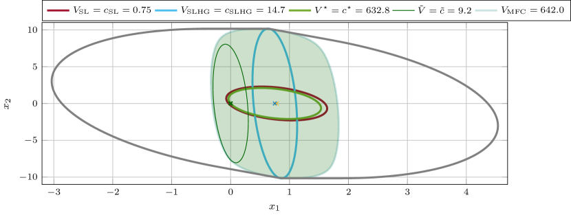
Figure 3: Estimated regions of attraction for $\bm{x}_{\mathrm{d}}=($0.75$\;0)^{\top}$ and $\bm{x}_{0}=\bm{0}$ and various control designs.

In Figure 3 the ruby ellipse is the maximum level-set $\Omega_{\mathrm{SL}}$ for the single-loop design in (54) satisfying (55), centred at the steady-state $\bm{x}_{\mathrm{s}}$ (marked in yellow) which has an offset to the set-point $\bm{x}_{\mathrm{d}}$ due to the uncertainty. The lightblue ellipse $V_{\mathrm{SLHG}}=c_{\mathrm{SLHG}}=$14.74$$ depicts the estimated region of attraction for the single-loop high-gain design (56). Note that the initial condition $\bm{x}_{0}=\bm{0}$ lies not within the estimated region of attraction of the single-loop high-gain design, thus we have no guarantee of convergence for this scenario. The green ellipse centred at $\bm{x}_{\mathrm{d}}$ shows the level-set of the Lyapunov function $V^{\star}$ for the MCL with $c^{\star}=$632.813$$. The level-set is chosen according to (47) such that it just covers the initial model state $\bm{x}^{\star}_{0}=\bm{0}$, i.e. $c^{\star}=\vartheta\tilde{\bm{x}}^{\star\top}_{0}\bm{P}\tilde{\bm{x}}^{\star}_{0}$.

In dark green we have the maximum set $\tilde{\Omega}$ in (48) satisfying (49) for this choice of $c^{\star}$. Note that $\tilde{\Omega}$ is defined for $\tilde{z}$, which describes an ellipse in the $(x_{1},x_{2})$-plane centred at $\bm{x}_{0}^{\star}+\tilde{\bm{x}}_{\mathrm{s}}$ for the initial states. Thus for any initial process state $\bm{x}_{0}\in\tilde{\Omega}$ we can guarantee asymptotic stability if we choose $\bm{x}^{\star}_{0}=\bm{0}$. In this sense the set $\tilde{\Omega}$ can be interpreted as robustness of the MFC with respect to an uncertain initial process state $\bm{x}_{0}$ for the chosen initial model state $\bm{x}^{\star}_{0}$. While $t>0$ increases, the centre of $\tilde{\Omega}$ moves along the solution $\bm{x}^{\star}(t)$ of the MCL offset by stationary error $\tilde{\bm{x}}_{\mathrm{s}}$, and represents the robustness of the MFC scheme w.r.t. the perturbed process state at any time instant $t\geq 0$ and also a bound for $\bm{x}(t)$, $t\geq 0$ in the closed-loop MFC scheme.

Of course different choices of $\bm{x}^{\star}_{0}$ yield different regions $\tilde{\Omega}$ for the initial process state $\bm{x}_{0}$. Considering $\bm{x}^{\star}_{0}$ as design parameter of the MFC restricted to $V^{\star}(\bm{x}^{\star}_{0})=$632.813$$ we can move the centre of $\tilde{\Omega}$ around the ellipse $V^{\star}$ offset by $\tilde{\bm{x}}_{\mathrm{s}}$, yielding the green-shaded area $\Omega_{\mathrm{MFC2}}$ for $c^{\star}+\tilde{c}=$642.045$$. This represents the region of attraction for the MFC scheme for $V^{\star}(\bm{x}^{\star}_{0})=$632.813$$, resulting in a much larger region than both single-loop designs.

We may also vary the choice of $c^{\star}$, i.e. the level of $V^{\star}(\bm{x}^{\star}_{0})$. We note that $c^{\star}$ decreases as $\bm{x}^{\star}_{0}$ approaches the set-point $\bm{x}_{\mathrm{d}}$, which allows for an increase of $\tilde{c}$ and thus the robustness w.r.t. the initial process state $\tilde{\Omega}$ increases. For $c^{\star}=0$, i.e. $\bm{x}^{\star}_{0}=\bm{x}_{\mathrm{d}}$, and with the weight $\vartheta\rightarrow\infty$ we get $V_{\mathrm{MFC}}=\tilde{V}=V_{\mathrm{SLGH}}$ as a special case. If we consider all possible pairs $c^{\star},\tilde{c}$ satisfying (46) we obtain the region of attraction for the initial process state $\bm{x}_{0}$ depicted by the grey line. This region is again considerably larger than both single-loop designs. Note, however, that some of these initial states require perfect knowledge of the initial process state such that $\bm{x}^{\star}_{0}=\bm{x}_{0}$ can be chosen. But in many cases we have a significant robustness with respect to the uncertain initial state $\bm{x}_{0}$ yielding again a much larger region of attraction.

Figure 4 shows several trajectories for $\bm{x}_{0}=\bm{0}$ and two additional trajectories for $\bm{x}_{0}\neq\bm{0}$. The yellow line (mostly covered) and purple line show the single-loop simulations. Remarkably, the single-loop high-gain approach shows convergence even though we have not shown stability for this initial condition. The yellow line is covered by the MFC solution $\bm{x}^{\star}$ (dashed red) as the MCL uses exactly the same control law as the single-loop design. Solid blue is the process state $\bm{x}$ for the MFC high-gain design which follows $\bm{x}^{\star}$ very closely. Additionally, we have included two further simulations of the MFC with perturbed initial process state in dashed and dash-dotted blue. This illustrates the robustness of the MFC towards uncertain initial states.

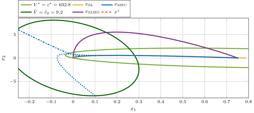
Figure 4: Phase portrait and estimated region of attraction for $\bm{x}_{\mathrm{d}}=($0.75$\;0)^{\top}$ and $\bm{x}_{0}=\bm{0}$. For the MFC scheme we have $\bm{x}^{\star}_{0}=\bm{0}$ with three different initial values of the process states: $\bm{x}_{0}=\bm{0}$ (solid blue line), $\bm{x}_{0}=(0.1\enspace-8)^{\top}$ (dotted blue line), and $\bm{x}_{0}=(-0.25\enspace 6)^{\top}$ (dashed-dotted blue line).

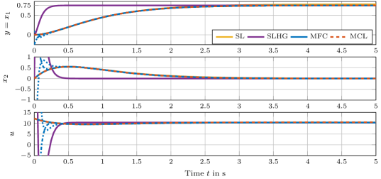
Figure 5: Time-responses of the states and input signal for $\bm{x}_{\mathrm{d}}=($0.75$\;0)^{\top}$ and $\bm{x}_{0}=\bm{0}$. For the MFC scheme we have $\bm{x}^{\star}_{0}=\bm{0}$ with three different initial values of the process states: $\bm{x}_{0}=\bm{0}$ (solid blue line), $\bm{x}_{0}=(0.1\enspace-8)^{\top}$ (dotted blue line), and $\bm{x}_{0}=(-0.25\enspace 6)^{\top}$ (dashed-dotted blue line).

The time response in Figure 5 shows that the MFC solutions are very similar to the standard single-loop design. However, the single-loop design has a large steady-state error of about [round-mode=none]4,3 whereas the steady-state error of the MFC scheme is negligible. We also observe that the deviations from the initial process state (dashed and dash-dotted lines) are rapidly compensated in the MFC scheme (less than [round-mode=none]0.5). The single-loop high-gain design (purple) shows a much faster convergence with identical (negligible steady-state error) at the expense of very large control effort $u_{\mathrm{SLGH}}(0)\approx$310$$. The MFC with the same initial process state only requires $u_{\mathrm{MFC}}(0)\approx$13$$. In this sense the MFC inherits the benefits of both single-loop designs: the steady-state performance of the high-gain design with moderate control effort of the simple single-loop design. Only if we move the initial process state to the extreme boundary of the estimated region of attraction we observe large control effort of $u_{\mathrm{MFC}}(0)\approx-127$ for $\bm{x}_{0}=(-0.25\enspace 6)^{\top}$, and even $u_{\mathrm{MFC}}(0)\approx 290$ for $\bm{x}_{0}=(0.1\enspace-8)^{\top}$.

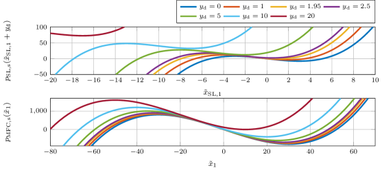
Figure 6: Functions $p_{\mathrm{SL},\mathrm{s}}(x_{1})$ and $p_{\mathrm{MFC},\mathrm{s}}(\tilde{x}_{1})$. They show the steady-state for $p_{\mathrm{SL},\mathrm{s}}(x_{\mathrm{s},1})=0$ and $p_{\mathrm{MFC},\mathrm{s}}(\tilde{x}_{\mathrm{s},1})=0$.

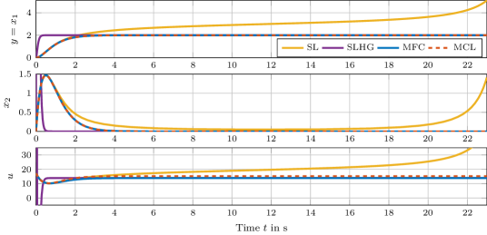
Figure 7: Time-response of states and input signal for $\bm{x}_{\mathrm{d}}=($2$\;0)^{\top}$ and $\bm{x}_{0}=\bm{x}^{\star}_{0}=\bm{0}$.

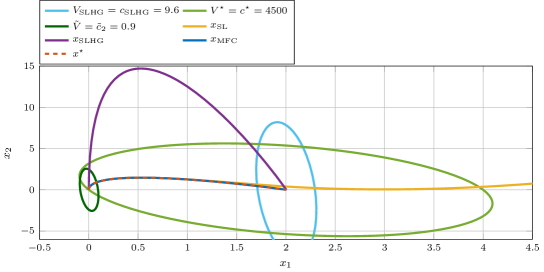
Figure 8: Phase portrait and estimated region of attraction for $\bm{x}_{\mathrm{d}}=($2$\;0)^{\top}$ and $\bm{x}_{0}=\bm{x}^{\star}_{0}=\bm{0}$.

The second scenario considers the desired state at $\bm{x}_{\mathrm{d}}=($2$\enspace 0)^{\top}$ and the initial states at $\bm{x}_{0}=\bm{x}^{\star}_{0}=\bm{0}$. For the single-loop design the uncertainty disturbs the steady-state (21) such that the set-point ceases to be an equilibrium. Defining $\tilde{\bm{x}}_{\mathrm{SL}}\coloneqq\bm{x}-\bm{x}_{\mathrm{d}}$ and substituting $x_{1}$ in Eq. (51) we obtain

$$\hskip-5.0ptp_{\mathrm{SL}}(\tilde{x}_{\mathrm{SL},1}+y_{\mathrm{d}})\!=\!k_{1}^{\star}\tilde{x}_{\mathrm{SL},1}-\left(\!\frac{\Delta k}{m}\left(\alpha+\Delta\alpha\right)^{2}(\tilde{x}_{\mathrm{SL},1}+y_{\mathrm{d}})^{3}\right.\\ \left.+\frac{k}{m}\Delta a\left(2\alpha+\Delta\alpha\right)(\tilde{x}_{\mathrm{SL},1}+y_{\mathrm{d}})^{3}+\frac{\Delta k}{m}(\tilde{x}_{\mathrm{SL},1}+y_{\mathrm{d}})\right).$$

The top plot of Figure 6 shows this polynomial for various values of the desired output $y_{\mathrm{d}}$. We observe that there are up to three possible solutions for the steady-state equation. However for a desired output references of $y_{\mathrm{d}}>$1.95$$, there remains only one solution for the considered uncertainty. The remaining steady-state is unstable. The plot at the bottom of Figure 6 depicts the function $p_{\mathrm{MFC}}(\tilde{x}_{1})$ given by Eq. (32) for the MFC scheme. We observe that the stable equilibria in terms of the error state $\tilde{x}_{1}$ remain close to zero for significantly larger values of $y_{\mathrm{d}}$. They are accompanied by unstable equilibria that are much further away than in the single-loop design. Note that the steady-state results of the MFC design are exactly the same for the single-loop high-gain design as discussed in Section 4.2.

Accordingly the single-loop design is not able to stabilise the desired state whereas the single-loop high-gain and the MFC high-gain design reach steady-state with negligible error, see Figure 7. Again the MFC requires significantly less control effort than the single-loop high-gain control $u(0)\approx$810$$. Figure 8 shows the phaseplane with the estimated regions of attraction. The initial condition $\bm{x}_{0}=\bm{0}$ is not within estimated the region of attraction for the single-loop high-gain design (lightblue). The robustness with respect to deviations of the initial conditions $\bm{x}_{0}$ and $\bm{x}^{\star}_{0}$ given by $\tilde{V}$ is smaller than in the first scenario. This is caused by a larger deviation of the model states to the desired states which requires a larger level-set $V^{\star}$ and allows only for smaller values of $\tilde{c}$ for the level-set of $\tilde{V}$.

References

- [1] G. Ambrosino, G. Celentano, and F. Garofalo. Robust model tracking control for a class of nonlinear plants. IEEE Transactions on Automatic Control, 30(3):275–279, 1985.
- [2] D. Bauer, U. Schaper, K. Schneider, and O. Sawodny. Observer design and flatness-based feedforward control with model predictive trajectory planning of a crane rotator. In American Control Conference, pages 4020–4025, 2014.
- [3] J. Brzózka. Modified model following control structure. Pomiary Automatyka Kontrola, 57(9):1052–1054, 2011.
- [4] J. Brzózka. Design of robust, nonlinear control system of the ship course angle, in a model following control (MFC) structure based on an input-output linearization. Scientific Journals Maritime University of Szczecin, 30(102):25–29, 2012.
- [5] Tzuen-Lih Chern and Geeng-Kwei Chang. Automatic voltage regulator design by modified discrete integral variable structure model following control. Automatica, 34(12):1575–1585, 1998.
- [6] Paweł Dworak, Krzysztof Pietrusewicz, and Stefan Domek. Improving stability and regulation quality of nonlinear MIMO processes. IFAC Proceedings Volumes, 42(13):180–185, 2009.
- [7] Heinz Erzberger. On the use of algebraic methods in the analysis and design of model-following control systems. Technical report, National Aeronautics and Space Administration, Washington DC, 1968.
- [8] Michel Fliess, Jean Lévine, Philippe Martin, and Pierre Rouchon. Flatness and defect of non-linear systems: introductory theory and examples. International Journal of Control, 61(6):1327–1361, 1995.
- [9] K. Graichen, M. Egretzberger, and A. Kugi. Suboptimal model predictive control of a laboratory crane. In Proc. of the 8th IFAC Symposium on Nonlinear Control Systems, pages 397–402, 2010.
- [10] Knut Graichen, Veit Hagenmeyer, and Michael Zeitz. A new approach to inversion-based feedforward control design for nonlinear systems. Automatica, 41(12):2033 – 2041, 2005.
- [11] Isaac M. Horowitz. Synthesis of feedback systems. Academic Press, 1963.
- [12] J. Huber, C. Gruber, and M. Hofbaur. Online trajectory optimization for nonlinear systems by the concept of a model control loop – Applied to the reaction wheel pendulum. In 2013 IEEE International Conference on Control Applications (CCA), pages 935–940, 2013.
- [13] Hassan K. Khalil. Nonlinear Systems. Prentice-Hall, 2002.
- [14] R. Osypiuk. Multi-loop model based parallel control systems. In 2010 IEEE/RSJ International Conference on Intelligent Robots and Systems (IROS), pages 1638–1643, 2010.
- [15] R. Osypiuk. Simple robust control structures based on the model-following concept – A theoretical analysis. International Journal of Robust and Nonlinear Control, 20(17):1920–1929, 2010.
- [16] Rafael Osypiuk and Torsten Kröger. A Three-Loop Model-Following Control Structure: Theory and Implementation. International Journal of Control, 83(1):97–104, 2010.
- [17] Tomasz Pajchrowski. Robust control of PMSM system using the structure of MFC. COMPEL - The international journal for computation and mathematics in electrical and electronic engineering, 30(3):979–995, 2011.
- [18] Krzysztof Pietrusewicz. Multi-degree of freedom robust control of the CNC XY table PMSM-based feed-drive module. Archives of Electrical Engineering, 61(1):15–31, 2012.
- [19] Günter Roppenecker. Zeitbereichsentwurf linearer Regelungen: Grundlegende Strukturen und eine allgemeine Methodik ihrer Parametrierung. Oldenbourg, 1990.
- [20] Günter Roppenecker. Zustandsregelung linearer Systeme – Eine Neubetrachtung. at - Automatisierungstechnik Methoden und Anwendungen der Steuerungs-, Regelungs- und Informationstechnik, 57(10):491–498, 2009.
- [21] Ulf Schaper. Schwingungsdämpfende Regelung der Pendel- und Schwenkdynamik von Hafenmobilkranen. PhD thesis, Institut für Systemdynamik der Universität Stuttgart, 2014.
- [22] Ulf Schaper, Eckhard Arnold, Oliver Sawodny, and Klaus Schneider. Constrained real-time model-predictive reference trajectory planning for rotary cranes. In IEEE/ASME International Conference on Advanced Intelligent Mechatronics, pages 680–685, 2013.
- [23] Ulf Schaper, Christina Dittrich, Eckhard Arnold, Klaus Schneider, and Oliver Sawodny. 2-DOF skew control of boom cranes including state estimation and reference trajectory generation. Control Engineering Practice, 33(12):63–75, 2014.
- [24] Stanisław Skoczowski. Robust model following control with use of a plant model. International Journal of Systems Science, 32(12):1413–1427, 2001.
- [25] Stanisław Skoczowski, Stefan Domek, and Krzysztof Pietrusewicz. Model following PID control system. Kybernetes, 32(5/6):818–828, 2003.
- [26] N. Tietze, K. Wulff, and J. Reger. Dynamic partial state-feedback revisited for output tracking using Lyapunov redesign and model-following control. In 63rd IEEE Conference on Decision and Control, 2024.
- [27] Niclas Tietze, Kai Wulff, and Johann Reger. A model-following control approach to peaking attenuation in the context of high-gain partial state feedback stabilisation of nonlinear systems. In 4th IFAC Conference on Modelling, Identification and Control of Nonlinear Systems, pages 7–12, Lyon, 2024.
- [28] Julian Willkomm. Model-Following Control for a Class of Nonlinear Systems. Dissertation, Technische Universität Ilmenau, 2023.
- [29] Julian Willkomm, Kai Wulff, and Johann Reger. Feedforward control for non-minimumphase local model networks using model following control. In 2018 IEEE Conference on Control Technology and Applications (CCTA), pages 1577–1582. IEEE, 2018.
- [30] Julian Willkomm, Kai Wulff, and Johann Reger. Tracking-control for the boost-pressure of a turbo-charger based on a local model network. In 2019 IEEE International Conference on Mechatronics (ICM), volume 1, pages 108–113. IEEE, 2019.
- [31] Julian Willkomm, Kai Wulff, and Johann Reger. Quantitative robustness analysis of model following control for nonlinear systems subject to model uncertainties. In 3rd IFAC Conference on Modelling, Identification and Control of Nonlinear Systems, pages 184–189, 2021.
- [32] Julian Willkomm, Kai Wulff, and Johann Reger. Set-point tracking for nonlinear systems subject to uncertainties using model-following control with a high-gain controller. In European Control Conference, pages 1617–1622, 2022.
- [33] Christoph Wurmthaler and Alexander Kühnlein. Modellgestützte vorsteuerung für messbare Störungen. at - Automatisierungstechnik, 57(7):328–331, 2009.