Topologically Charged Vortices at Superconductor/Quantum Hall Interfaces

Abstract

We explore interface states between a type-II $s$-wave superconductor (SC) and a Chern insulator in the integer quantum Hall (QH) regime. Our results show that the effective interaction at this boundary gives rise to two emergent Abelian Higgs fields, representing paired electrons at the SC/QH interface. These fields couple to a gauge field that includes both Chern-Simons term, originating from the QH sector, and Maxwell term. Using this framework, we investigate the effects of magnetic flux vortices on the SC/QH interface. The emergence of the Chern-Simons term significantly modifies the magnetic penetration depth, influencing the Abrikosov lattice period and potentially altering the superconducting behavior at the interface. Furthermore, we demonstrate that vortex solutions at the interface carry a fractional charge of $e/2$, which reflects the ratio between the effective Chern-Simons level parameter and the charge of the Cooper pairs.

Introduction: Superconductivity is a quantum effect arising from the spontaneous symmetry breaking (SSB) of the $U(1)$ symmetry and a phase transition driven by the Higgs mechanism. In this framework, the superconducting order parameter is pinned to a minimum of a Higgs potential in a Ginzburg-Landau theory, which emerges by integrating out the fermionic degrees of freedom in the microscopic Bardeen-Cooper-Schrieffer (BCS) action.

Superconductors can be classified into two main types based on the relation between two important length scales: the coherence length $\xi$ governs the spatial extent of Coopers pairs and is inversely related to the Higgs mass. Moreover, the penetration depth $\lambda$ is inversely related to the mass of the gauge boson after SSB, and governs the decay of magnetic fields inside the superconductor. Type-I superconductors ($\sqrt{2}\lambda<\xi$) completely expel the magnetic field and thus exhibit a strong Meissner effect. In contrast, type-II superconductors ($\sqrt{2}\lambda>\xi$) allow the magnetic field to penetrate into the superconductor in the form of quantized flux vortices.

These vortices have been extensively studied within the framework of the Ginzburg-Landau theory [1, 2, 3] and its relativistic generalization, the Abelian Higgs model [4], where they are electrically neutral. However, the inclusion of a Chern-Simons (CS) term alters this picture by introducing a topological charge to the vortices, determined by the ratio of the effective CS level parameter to the charge of the complex scalar field [5, 6, 7]. Consequently, in the case of Cooper pairs, this charge becomes fractional [8].

In this Letter, we investigate the interface between a type-II $s$-wave superconductor (SC) and a Chern insulator, which exhibits the integer quantum Hall (QH) effect. This experimentally well-established configuration [9, 10, 11, 12, 13] provides a rich platform for exploring novel excitations arising from the coupling between superconductivity and topological edge states [14, 15, 16, 17, 18]. Specifically, we show that the effective theory describing the interface interaction can be modeled by two coupled Abelian Higgs fields, corresponding to the paired electrons at the SC/QH interface, along with an emergent CS term. This interaction brings about novel phenomena at the interface, including a topological mass for the gauge boson, which affects the magnetic penetration depth and a topological charge for the vortices.

The change of the magnetic penetration depth directly influences the vortex lattice period and the type of superconductivity at the interface. Depending on the system parameters, this interaction can increase the lattice period and drive a transition between type-II and type-I superconductivity. Furthermore, the vortices at the interface acquire fractional charge, as the scalar pairs carry twice the charge of a fermion. This distinguishes them from both conventional superconducting vortices and those governed by the standard CS term in the Abelian Higgs model. This fractional charge raises the intriguing possibility that these vortices are a realization of anyons, i.e., particles that obey fractional statistics.

In this work, we provide a detailed analysis of the interface states and the novel features emerging from the coupling between the SC and the QH system, using the framework of quantum field theory. Throughout the Letter, we will consider a $2+1$ dimensional spacetime for the QH system with the metric $g^{\mu\nu}=(+,-,-)$ and the Levi-Civita symbol $\epsilon^{012}=\epsilon_{012}=+1$. The superconductor, on the other hand, lives in a $3+1$ dimensional spacetime. The contravariant vector is denoted as $x^{\mu}=(t,x,y,z)$. We adopt natural units where $\hbar=c=1$, and employ the Feynman slash notation, $\not{A}=\gamma^{\mu}A_{\mu}$, where the $\gamma$ matrices in the 2+1 and 3+1 dimensional systems are defined in Supplemental Material (SM). Additionally, $\bar{\psi}=\psi^{\dagger}\gamma^{0}$ and $\psi^{T}$ denotes the transpose of the corresponding spinor.

Effective Action: We consider the following total action for the combined SC/QH system,

$$S=S_{\rm QH}+S_{\rm SC}+S_{\rm int}+S_{\rm Maxwell}\,.$$ (1)

The first term describes the action for the QH sector. Our effective field theory is independent of the microscopic details of the electronic model, but to be specific we can consider for simplicity a Chern insulator, i.e., a lattice model with non-vanishing Chern number which shows an integer quantum Hall effect. The simplest such two-dimensional lattice Hamiltonian is $\sum_{\boldsymbol{k}}C_{\boldsymbol{k}}^{\dagger}(v_{F}\,\boldsymbol{\sigma}\cdot\boldsymbol{k}+m_{q}v_{F}^{2}\sigma_{z})C_{\boldsymbol{k}}$, where $v_{F}$ is the Fermi velocity, $\boldsymbol{\sigma}=(\sigma_{x},\sigma_{y},\sigma_{z})$ is the vector of Pauli matrices and the two-component operators $C_{\boldsymbol{k}}$ represent states in two bands with the momentum $\boldsymbol{k}=(k_{x},k_{y})$. The mass term $m_{q}v_{F}^{2}\sigma_{z}$ breaks time-reversal symmetry and opens a gap in the spectrum. The energy spectrum can be written as $\epsilon_{q}(\boldsymbol{k})=\pm\sqrt{(v_{F}\boldsymbol{k})^{2}+(m_{q}v_{F}^{2})^{2}}$ and in the limit of $m_{q}\to 0$, $\epsilon_{q}(\boldsymbol{k})=\pm v_{F}|\boldsymbol{k}|$, corresponding to the Dirac cone.

In the continuum limit, this Hamiltonian corresponds to that of a $2$-component Dirac fermion in $2+1$ dimensions. By further considering the orbital effect of a applied magnetic field, we obtain the $2+1$ dimensional action for the Dirac field with mass $m_{q}v_{F}^{2}$ coupled to a classical background gauge field $A_{\mu}(t,x,y)$,

$$S_{\rm QH}=\int d^{3}x\,\bar{\psi}_{q}(i\not{D}-m_{q}v_{F}^{2})\psi_{q}\,,$$ (2)

where we parametrize the quantum field as $v_{F}\psi_{q}(t,v_{F}x,v_{F}y)$. It can be expanded in terms of Grassmann variables in the basis of 2-component spinors, and $D_{\mu}=\partial_{\mu}+ieA_{\mu}$ is the covariant derivative for the gauge field $A_{\mu}$ with the charge $e$. We note that the disappearance of the Fermi velocity in the spatial derivatives stems from the relation $v_{F}\partial_{i}\psi_{q}(t,x,y)=\partial_{i}\psi_{q}(t,v_{F}x,v_{F}y)$, see SM.

To describe the SC sector at the microscopic level, we start from the BCS action for the fermionic field $\varphi_{\uparrow,\downarrow}(t,x,y,z)$,

$$S_{\rm BCS}=\int dtdxdydz \bigg{[}\sum_{\sigma=\uparrow,\downarrow}\varphi_{\sigma}^{*}\left(i\partial_{t}+\frac{\boldsymbol{\nabla}^{2}}{2m_{s}}+\mu\right)\varphi_{\sigma}$$

$$+g\,\varphi_{\uparrow}^{*}\varphi_{\downarrow}^{*}\varphi_{\downarrow}\varphi_{\uparrow}\bigg{]},$$ (3)

where $\mu$ is the chemical potential and $g$ denotes the strength of the phonon-mediated interaction between electrons, which leads to formation of Cooper pairs below a critical temperature. The BCS action yields the phenomenological Ginzburg–Landau description of superconductivity when integrated over the fermionic degrees of freedom. In principle, one can use the above BCS action, by coupling it to the gauge field $A_{\mu}$, for the SC sector in our model. However, since the action describing the QH sector is in relativistic form, it is beneficial for the calculation to approximate the BCS action with its relativistic form. For this purpose, we introduce the following $3+1$ dimensional action for the Dirac field $v_{F}^{3/2}\psi_{s}(t,v_{F}x,v_{F}y,v_{F}z)$ coupled to the gauge field $A_{\mu}(t,x,y,z)$:

$$S_{\rm SC}=\int d^{4}x \bigg{[}\bar{\psi}_{s}(i\not{D}-\tilde{m}_{s}v_{F}^{2}+m_{s}v_{F}^{2}\gamma^{0})\psi_{s}$$

$$+g\,\psi^{T}_{s}\xi_{s}\psi_{s}\,\bar{\psi}_{s}\xi^{\dagger}_{s}\bar{\psi}^{T}_{s}\bigg{]}\,.$$ (4)

Here $\tilde{m}_{s}v_{F}^{2}=m_{s}v_{F}^{2}\sqrt{1-2\mu/(v_{F}^{2}m_{s})}$ and for simplicity we assume that the Fermi velocities are identical in both the SC and QH sectors. The field $\psi_{s}$ can be expanded in the basis of $4$-compenent spinors with Grasmann coefficients. The last term is a four-fermion interaction, where $\xi_{s}=i\sigma_{y}/2\otimes I_{2}$, and corresponds to $s$-wave pairing in the mean-field approximation [19, 20]. Note that the energy is expressed as $\epsilon_{s}(\boldsymbol{k})=\sqrt{(v_{F}\boldsymbol{k})^{2}-(v_{F}k_{F})^{2}+(m_{s}v_{F}^{2})^{2}}-m_{s}v_{F}^{2}$, which approximates to $|\epsilon_{s}(\boldsymbol{k})|\approx\boldsymbol{k}^{2}/(2m_{s})-\mu$ with $k_{F}=\sqrt{2m_{s}\mu}$ in the limit $\sqrt{|k^{2}-k_{F}^{2}|}\ll m_{s}v_{F}$.

The third term of the action (1) describes the surface interaction between the SC and QH electrons. Suppose that an $s$-wave superconductor is deposited on the surface, allowing Cooper pairs to tunnel into the surface states due to the proximity effect [21]. As a result, we can consider a pair-pair interaction at the interface. Accordingly, we identify the interaction term as

$$S_{\rm int}=\eta\int d^{4}x\,\delta(z)(\psi_{s}^{T}\xi_{s}\psi_{s}\,\bar{\psi}_{q}\xi_{q}^{\dagger}\bar{\psi}^{T}_{q}+\text{h.c.})\,,$$ (5)

with an effective interaction strength $\eta$, which is typically small compared to the bare pairing strength, $\eta<g$. Here $\xi_{q}=i\sigma_{y}/2$ is the $s$-wave pairing matrix for the electrons at the QH sector and the Dirac delta function confines the SC sector to the $x-y$ plane to describe the interaction of the SC and QH electron pairs at the interface. Finally, the last term is the usual Maxwell action, given by

$$S_{\rm Maxwell}=-\frac{1}{4}\int d^{4}x\,F_{\mu\nu}F^{\mu\nu}\,,$$ (6)

with $F_{\mu\nu}=\partial_{\mu}A_{\nu}-\partial_{\nu}A_{\mu}$ being the electromagnetic tensor.

In order to derive an effective theory for the interface, we integrate over all fermionic degrees of freedom by considering the path integral,

$$Z[A]=\int D(\bar{\psi}_{s},\psi_{s})D(\bar{\psi}_{q},\psi_{q})e^{iS}\,.$$ (7)

After a series of manipulations, shown in SM, the path integral can be written as

$$Z[A]=\int D(\bar{\phi_{1}},\phi_{1})D(\bar{\phi_{2}},\phi_{2})e^{iS_{\rm eff}}\,,$$ (8)

with the effective action

$$S_{\rm eff}=\frac{k}{4\pi}\int d^{3}x\,\varepsilon^{\mu\nu\rho}A_{\mu}\partial_{\nu}A_{\rho}-\frac{1}{4}\int d^{3}x\,F_{\mu\nu}F^{\mu\nu}$$ (9)

$$+\int d^{3}x\,\sum_{i=1}^{2}\left[\left|(\partial_{\mu}+iqA_{\mu})\phi_{i}\right|^{2}-\lambda_{i}\left(|\phi_{i}|^{2}-\frac{\sigma_{i}^{2}}{2}\right)^{2}\right].$$

The second line of the action arises from the four-fermion interactions in the SC sector (Topologically Charged Vortices at Superconductor/Quantum Hall Interfaces) and the interface interaction (5) and contains the Hubbard-Stratonovich fields $\phi_{1}$ and $\phi_{2}$. We assume translational symmetry along the $z$-direction in the SC sector, which allows us to confine the action to the interface in $2+1$ dimensions [2]. Through a saddle-point approximation, equivalent to a mean-field approximation, it is established that these fields represent electron pairs in the SC and QH sectors, respectively, with a charge of $q=2e$: $\phi_{1,\rm MF}=g\braket{\psi_{s}^{T}\xi_{s}\psi_{s}}+\eta\braket{\psi^{T}_{q}\xi_{q}\psi_{q}}\approx g\braket{\psi_{s}^{T}\xi_{s}\psi_{s}}$ and $\phi_{2,\rm MF}\approx\eta^{2}\braket{\psi^{T}_{q}\xi_{q}\psi_{q}}/(gL_{\rm QH})$ with a short-distance cutoff $L_{\rm QH}$ corresponding to the thickness of the QH layer (see SM). The parameters $\lambda_{i}>0$ and $\sigma_{i}>0$ represent the coefficients arising in the perturbative expansion of the interaction term after the Hubbard-Stratonovich transformation.

The first term of Eq. (9) is a CS term resulting from integrating over the fermionic field of the QH sector. This can be understood by noting that in a $2+1$ dimensional spacetime, the trace of three gamma matrices does not vanish and is given by $\operatorname{Tr}(\gamma^{\mu}\gamma^{\nu}\gamma^{\rho})=2i\epsilon^{\mu\nu\rho}$, which emerges from the one-fermion loop. The parameter $k/e^{2}=1$ is known as the level parameter of the CS term, while $k=e^{2}$ can be referred to as the effective level parameter. The second term in the first line is the Maxwell action confined to the $2+1$ dimensions.

In physical terms, the effective action (9) describes the interaction of two species of electron pairs, represented by scalar fields $\phi_{1}$ and $\phi_{2}$, via the gauge field $A_{\mu}$, in the presence of both CS and Maxwell terms. From here on, we will refer to this effective action as the coupled Abelian Higgs-Chern-Simons (HCS) action: $S_{\rm eff}=S_{\rm HCS}$.

Spontaneous Symmetry Breaking: In the absence of the QH sector (i.e., when $\phi_{2}\to 0$ and $k\to 0$), the HCS action Eq. (9) reduces to the well-known Ginzburg-Landau action (or Abelian Higgs action in the terminology of high-energy physics). The potential energy term $\lambda_{1}(|\phi_{1}|^{2}-\sigma_{1}^{2}/2)^{2}$ reaches its minimum at $|\phi_{1}|=\sigma_{1}/\sqrt{2}$. As a result, the field $\phi_{1}$ settles into this minimum, breaking the global $U(1)$ symmetry and forming the superconducting state. This transition introduces the gap $\sigma_{1}/\sqrt{2}$ at the mean-field level, distinguishing the superconducting state from the normal state, where $\phi_{1}=0$. In the superconducting state, one can define the Landau parameter $\kappa=\lambda_{L}/\xi_{L}$, where $\lambda_{L}=1/(q\sigma_{1})$ represents the penetration depth of the magnetic field and $\xi_{L}=1/(\sigma_{1}\sqrt{\lambda_{1}})$ denotes the coherence length of $|\phi_{1}|$. For $\kappa<1/\sqrt{2}$, corresponding to type-I superconductors, $\sqrt{2}\lambda_{L}<\xi_{L}$ resulting in the magnetic field being entirely expelled (the Meissner effect). In contrast, $\kappa>1/\sqrt{2}$ defines type-II superconductors, where the magnetic field can penetrates into the SC in the form of vortex lines [22].

We can analyze the full HCS action (9) in a similar way within the framework of SSB. Accordingly, we introduce two Higgs bosons $H_{1,2}(x)$ and a single Goldstone boson $G(x)$ into the model. The latter emerges as a consequence of the gauge invariance of the action. The fields $\phi_{i}$ can then be expanded around their vacuum expectation values as follows,

$$\phi_{i}=\frac{1}{\sqrt{2}}(\sigma_{i}+H_{i}(x))e^{iG(x)}\,.$$ (10)

Using the gauge transformation $A_{\mu}\to A_{\mu}-\partial_{\mu}G/q$, known as the unitary gauge, the massless Goldstone boson disappears. The HCS Lagrangian density then describes the interactions between the two Higgs bosons and a single massive gauge boson,

$$\mathcal{L}_{\rm HCS}=\sum_{i=1}^{2}\left\{\frac{1}{2}\partial_{\mu}H_{i}\partial^{\mu}H_{i}-\lambda_{i}\sigma_{i}^{2}H_{i}^{2}\right\}+\mathcal{L}_{\rm HCS}^{\rm int}(H_{i},A)$$ (11)

$$-\frac{1}{4}F_{\mu\nu}F^{\mu\nu}+\frac{k}{4\pi}\varepsilon^{\mu\nu\rho}A_{\mu}\partial_{\nu}A_{\rho}+\frac{1}{2}q^{2}(\sigma_{1}^{2}+\sigma_{2}^{2})A_{\mu}A^{\mu}\,,$$

where the second line can be identified as the Proca-Chern-Simons Lagrangian density, and $\mathcal{L}_{\rm HCS}^{\rm int}$ describes the interaction between the Higgs bosons and the massive gauge boson. In this Lagrangian density, the masses of the two Higgs bosons and the massive gauge boson are given by, respectively,

$$m_{H_{i}} =\sigma_{i}\sqrt{2\lambda_{i}}\,,$$

$$m_{G_{\pm}} =\sqrt{q^{2}(\sigma_{1}^{2}+\sigma_{2}^{2})+k^{2}/16\pi^{2}}\pm k/4\pi\,,$$ (12)

and the latter determines the equations of motion of the Proca-Chern-Simons Lagrangian density [23],

$$(\partial^{2}+m_{G_{+}})(\partial^{2}+m_{G_{-}})A^{\nu}=0\,.$$ (13)

It is important to note that the term $k/(4\pi)$, known as the topological mass, arises due to the presence of the CS term and renormalizes $m_{G\pm}$.

These masses allow us to identify the characteristic length scales arising naturally from the corresponding equations of motion. Specifically, in the static case, the fields behave as $H_{i}\sim\exp(-m_{H_{i}}r/\sqrt{2})$ and $A^{\nu}\sim\exp(-m_{G_{\pm}}r)$. Therefore, the respective coherence lengths of the fields $|\phi_{i}|$ are given by (for $i=1,2$),

$$\xi_{L_{i}}=\frac{\sqrt{2}}{m_{H_{i}}}=\frac{1}{\sigma_{i}\sqrt{\lambda_{i}}}\,,$$ (14)

while the penetration depth of the magnetic field is

$$\lambda_{L_{-}}=\frac{1}{m_{G_{-}}}=\frac{1}{\sqrt{q^{2}(\sigma_{1}^{2}+\sigma_{2}^{2})+k^{2}/16\pi^{2}}-k/4\pi}\,.$$ (15)

Note that $\lambda_{L_{-}}$ has been selected over $\lambda_{L_{+}}$ because the larger penetration depth $\lambda_{L_{-}}>\lambda_{L_{+}}$ give rise to an energetically favorable vortex [7].

At this point, we would like to emphasize that in the absence of the QH sector, $\phi_{2}\to 0$ and $k\to 0$, the penetration depth simplifies to $\lambda_{L_{-}}\to\lambda_{L}=1/(q\sigma_{1})$, consistent with the conventional Ginzburg-Landau theory previously discussed. However, a crucial distinction arises due to the CS term: while $\sigma_{2}$, which is governed by the interaction strength $\eta$ between the SC and QH sectors, may become negligible by tuning $\eta$, the terms proportional to $k$ persist even for small values of $\eta$. This persistence is a direct consequence of the topological nature of the CS term, which can significantly influence the penetration depth and thus the type of superconductivity induced at the interface, as we discuss now.

To illustrate this point, we introduce the following new parameters analogous to the Landau parameter,

$$\kappa_{i}=\lambda_{L_{-}}/\xi_{L_{i}}\,,$$ (16)

which characterize the type of superconductivity at the interface based on the distinction $\kappa_{i}\gtrless 1/\sqrt{2}$. Since the bulk superconductor is of type-II in the absence of the QH sector, the condition $\kappa>1/\sqrt{2}$ must be satisfied. This requirement imposes the physical constraint $\lambda_{1}>q^{2}/2$ within our model. Additionally, assuming $\eta<g$, another constraint emerges in the form $\sigma_{2}<\sigma_{1}$.

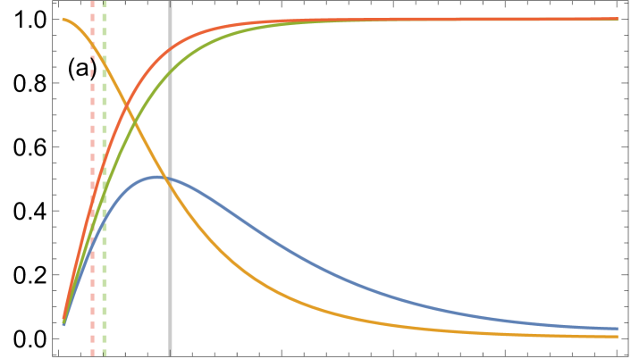
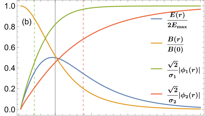
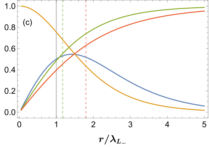
Figure 1: Numerical solutions of the vortex solutions (17) (see also Eq. (82) in SM) with $n=1$ and $e=1$. The applied parameters are as follows: (a) $\sqrt{2}\kappa_{1}=2.42$, $\sqrt{2}\kappa_{2}=3.27$ with $\sqrt{2}\kappa=2.73$, $\sigma_{2}/\sigma_{1}=0.62$; (b) $\sqrt{2}\kappa_{1}=2.35$, $\sqrt{2}\kappa_{2}=0.56$ with $\sqrt{2}\kappa=2.23$, $\sigma_{2}/\sigma_{1}=0.24$; (c) $\sqrt{2}\kappa_{1}=0.85$, $\sqrt{2}\kappa_{2}=0.55$ with $\sqrt{2}\kappa=1.02$, $\sigma_{2}/\sigma_{1}=0.66$. In the figures, the gray vertical lines represent the scaled penetration depths, while the dashed lines denote $1/(\sqrt{2}\kappa_{1})$ and $1/(\sqrt{2}\kappa_{2})$. A dashed line to the left of a gray line indicates type-II behavior; otherwise, it corresponds to type-I.

Vortex solutions: In the absence of the QH sector, the pair $(\phi_{1},A^{\mu})$ has vortex solutions, which are a hallmark of type-II superconductors. Furthermore, due to the gauge invariance of the total HCS action, the action must also admit a vortex solution for the pair $(\phi_{2},A^{\mu})$ to minimize the energy functional in the limit of $|\boldsymbol{x}|\to\infty$ [24] (see SM). To explore the pairs of vortex solutions, we build on the expansion around their vacuum expectation values (10), where the phase generates the gauge potential $A_{\theta}$, and thereby introduce the following ansatz, corresponding to a rotationally symmetric electric and magnetic field profile,

$$\phi_{i}=e^{in\theta}f_{i}(r)\,,\ A_{\theta}=A(r)/r\,,\ A_{r}=0\,,\ A_{0}=A_{0}(r)\,,$$ (17)

subject to the following appropriate boundary conditions: $\lim_{r\to\infty}f_{i}(r)=\sigma_{i}/\sqrt{2}$, $\lim_{r\to\infty}A(r)=n/q$, $\lim_{r\to\infty}A_{0}(r)=0$, $\lim_{r\to 0}f_{i}(r)=\lim_{r\to 0}A(r)=0$, and $\lim_{r\to 0}A_{0}(r)=A_{0}$. Here the constant $A_{0}$ can be specified such that the electric field in the limit of $r\to 0$ vanishes. Moreover, the integer $n$ is the winding number, and the flux $\Phi=-2\pi n/q$ classifies the finite energy solutions in terms of their winding number. We would like to point out that in the absence of the QH sector ($f_{2}=0$ and $k=0$, the latter also implies $A_{0}=0$) the ansatz precisely reduces to the one for the Nielsen-Olesen vortex solution [4]. However, unlike the Nielsen-Olesen vortex, the presence of the CS term endows the vortex with a topological charge. This can be demonstrated via the corresponding equations of motion, which can be expressed as

$$\boldsymbol{\nabla}\cdot\boldsymbol{E}+\frac{k}{2\pi}B=j^{0}\,,$$ (18)

see SM. Hence, the charge is

$$Q=\int d^{2}x\,j_{0}=\frac{k}{2\pi}\Phi=-n\,k/q=-n\,e/2\,.$$ (19)

This leads to the crucial conclusion that, for an odd winding number, the vortex possesses a fractional charge. This fractional charge emerges from the coupling of the CS term to electron pairs, which effectively carry twice the charge of a single fermion. This result indicates that the vortex formed at the SC/QH interface carries a fractional charge, even in the case of integer quantum Hall states.

Numerical calculations and experimental observables: It is known that except for certain special cases there is no analytical solution to the vortex equations presented in SM [25]. However, we can provide a set of numerical solutions for various parameters, as illustrated in Fig. 1. Fig. 1(a) illustrates a case where both pairs are affected by the penetrating magnetic field, with $\sqrt{2}\kappa_{1}=2.42$ and $\sqrt{2}\kappa_{2}=3.27$. In contrast, in Fig. 1(b) the superconducting pair experiences the magnetic field with a parameter value of $\sqrt{2}\kappa_{1}=2.35$, whereas the QH pair does not as $\sqrt{2}\kappa_{2}=0.56$. Interestingly, a third scenario exists in which the bulk superconductor, despite being type-II, behaves like a type-I at the interface with the parameters $\sqrt{2}\kappa_{1}=0.85$ and $\sqrt{2}\kappa_{2}=0.55$, and neither pair feels the magnetic field, see Fig. 1(c). Notably, a fourth possibility is ruled out as it violates the condition $\eta<g$.

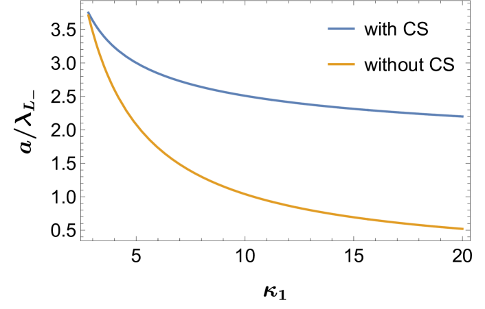
Figure 2: The change in the Abrikosov lattice period at the interface due to the QH sector for $n=1$ with $e=1$. The parameters used are $\sigma_{2}=0.01$, indicating a very weak interaction, and $\kappa_{1}$ ranges from 2.8 to 20 with $\lambda_{1}=30$, placing the system in the type-II superconducting regime. As shown in the figure, the presence of the CS term leads to an increase in lattice period, particularly for $\kappa_{1}\gg 1$.

All these numerical results can also be experimentally verified. It is well-established that vortices repel each other in the regime of type-II superconductivity [26]. Furthermore, this repulsion causes the vortices to form Abrikosov lattices which minimize the energy functional (see Eq. (80) in SM) [1]. For instance, the largest lattice period in a triangular lattice is given by [27]

$$a=\sqrt{\frac{2\Phi_{0}}{\sqrt{3}H_{c_{1}}}}\,,$$ (20)

where $\Phi_{0}=2\pi/q$ is the magnetic flux quantum, and $H_{c_{1}}\approx\Phi_{0}\ln(\lambda_{L_{-}}/\xi_{L_{i}})/(4\pi\lambda_{L_{-}}^{2})$ is the lower critical field. In the presence of the QH sector, the lattice period undergoes significant changes at the interface. In Fig. 2, we show that even for small coupling $\eta$, the lattice period increases due to the topological nature of the CS term. This finding provides a potential avenue for experimental verification of the predicted result. Consequently, the parameter regimes defined in Fig.1(a) and Fig.1(b) can be experimentally observed. On the other hand, for Fig. 1(c), we are in the regime of a type-I superconductor, where the Abrikosov lattice disappears, which can also be experimentally verified.

Conclusion. In summary, we have studied the interface between a type-II $s$-wave superconductor and a Chern insulator in the integer quantum Hall sregime. We showed that the interaction at this interface can be modeled using two Abelian Higgs fields coupled to a gauge field, which includes both an emergent Chern-Simons term and the Maxwell term. The presence of the Chern-Simons term significantly alters the magnetic field penetration depth at the interface, and hence the length scales of the Abrikosov lattice. Moreover, although the considered bulk superconductor is a type-II superconductor, the interaction with the QH sector can change the type of superconductivity at the interface. Finally, due to the interaction between the electron pairs and the Chern-Simons term, the emerging vortices at the interface carry a fractional charge.

Appendix A Supplemental Material

A.1 Emergence of the Chern-Simons Term

In the continuum limit, the action of the simplest two-dimensional lattice system, exhibiting an integer quantum Hall effect (QH), can be modeled with the action of a Dirac field $\psi_{q}$ of mass $m_{q}$

$$S_{\rm Dirac}=\int dt\,d^{2}x\,\bar{\psi}_{q}(t,x,y)\left(i\gamma^{0}\partial_{t}+iv_{F}\gamma^{i}\partial_{i}-m_{q}v_{F}^{2}\right)\psi_{q}(t,x,y)\,,$$ (21)

where $v_{F}$ is the Fermi velocity, and $\gamma^{0}=-\sigma_{z}$ and $\gamma^{1,2}=-i\sigma_{x,y}$ are the gamma matrices. Note that the energy can be written as $\epsilon_{q}(\boldsymbol{k})=\pm\sqrt{(v_{F}\boldsymbol{k})^{2}+(m_{q}v_{F}^{2})^{2}}$, and in the limit of $m_{q}\to 0$, $\epsilon_{q}(\boldsymbol{k})=\pm v_{F}|\boldsymbol{k}|$, corresponding to the Dirac cone.

The Dirac action (21) can be further expressed as

$$S_{\rm Dirac} =\int cdt\,d^{2}x\,\bar{\psi}_{q}(t,x,y)\left(i\gamma^{0}\partial_{0}+i\frac{v_{F}}{c}\gamma^{i}\partial_{i}-m_{q}\frac{v_{F}^{2}}{c}\right)\psi_{q}(t,x,y)$$

$$=\frac{v_{F}^{2}}{c^{2}}\int d^{3}x^{\prime}\,\bar{\psi}_{q}(t,x^{\prime}\,v_{F}/c,y^{\prime}\,v_{F}/c)\left(i\gamma^{0}\partial_{0}+i\gamma^{i}\partial^{\prime}_{i}-m_{q}\frac{v_{F}^{2}}{c}\right)\psi_{q}(t,x^{\prime}\,v_{F}/c,y^{\prime}\,v_{F}/c)$$

$$=\int d^{3}x\,\bar{\psi}_{q}^{\prime}(t,x,y)(i\gamma^{\mu}\partial_{\mu}-m_{q}v_{F}^{2})\psi_{q}^{\prime}(t,x,y)\,.$$ (22)

Here we define $\psi_{q}^{\prime}(t,x,y)=(v_{F}/c)\,\psi_{q}(t,x\,v_{F}/c,y\,v_{F}/c)$ with $c=1$. Furthermore, after we couple the Dirac field to a non-dynamical $U(1)$ gauge field $A_{\mu}(t,x,y)$, the action can be expressed as

$$S_{\rm QH}=\int d^{3}x\,\bar{\psi}_{q}\left(i\not{\partial}-e\not{A}-m_{q}v_{F}^{2}\right)\psi_{q}\,.$$ (23)

where we omit the primes. The two-component spinors $\psi_{q}(t,x,y)$ can be expanded in terms of Grassmann variables $\eta_{n}$ as

$$\psi_{q}(t,x,y)=\sum_{n}\eta_{n}\chi_{n}(t,x,y)\,,$$ (24)

where $\chi_{n}(t,x,y)$ denotes a complete basis of eigenstates of the Dirac equation. The corresponding path integral is given by

$$Z[A]=\int D(\bar{\psi}_{q},\psi_{q})e^{iS_{\rm QH}}=N\det M\,,$$ (25)

where $N$ is a normalization factor (see below) and

$$M=-i\not{\partial}+e\not{A}+m_{q}v_{F}^{2}=G_{0}^{-1}(1+ieS_{F}\not{A})\,.$$ (26)

Here, $G_{0}^{-1}=-i\not{\partial}+m_{q}v_{F}^{2}$ denotes the differential operator of the unperturbed massive Dirac field and

$$S_{F}(x-y)=\int d^{3}p\frac{i(\not{p}+m_{q}v_{F}^{2})}{p^{2}-(m_{q}v_{F}^{2})^{2}+i0^{+}}e^{-ip(x-y)}\,$$ (27)

is the Feynman propagator, i.e., the time-ordered Green’s function, which satisfies

$$\left(-i\not{\partial}_{x}+m_{q}v_{F}^{2}\right)_{\alpha\beta}[S_{F}(x-y)]_{\beta\gamma}=-i\delta_{\alpha\gamma}\delta^{(3)}(x-y)\,.$$ (28)

By choosing the normalization as $N=(\det G_{0}^{-1})^{-1}$ such that $Z[0]=1$, the path integral can be written as

$$Z[A]=\exp\left(-\sum_{n=1}^{\infty}\frac{(-e)^{n}}{n}\operatorname{Tr}(iS_{F}\not{A})^{n}\right)\,,$$ (29)

where the trace can be evaluated via

$$\operatorname{Tr}(iS_{F}\not{A})^{n}=i^{n}\int d^{3}x_{1}d^{3}x_{2}\cdots d^{3}x_{n}\operatorname{Tr}\not{A}(x_{1})S_{F}(x_{2}-x_{1})\not{A}(x_{2})S_{F}(x_{3}-x_{2})\cdots\not{A}(x_{n})S_{F}(x_{1}-x_{n})\,.$$ (30)

By writing $Z[A]=e^{iS_{\rm eff}[A]}$, the leading term of the effective action $S_{\rm eff}[A]$ can be expressed as

$$iS_{\rm eff}[A] =\frac{e^{2}}{2}\int d^{3}x_{1}d^{3}x_{2}\operatorname{Tr}\not{A}(x_{1})S_{F}(x_{2}-x_{1})\not{A}(x_{2})S_{F}(x_{1}-x_{2})=-\frac{e^{2}}{2}\int d^{3}p\,\tilde{A}_{\mu}(-p)\Pi^{\mu\nu}(p)\tilde{A}_{\nu}(p)\,,$$ (31)

where $\tilde{A}_{\mu}$ is the Fourier transform of the gauge field $A_{\mu}$ and $\Pi^{\mu\nu}$ is the polarization tensor arising from the one-loop Feynman diagram

$$\Pi^{\mu\nu}(p) =\operatorname{Tr}\int d^{3}k\,\gamma^{\mu}\frac{\not{k}-\not{p}+m_{q}v_{F}^{2}}{(k-p)^{2}-(m_{q}v_{F}^{2})^{2}+i0^{+}}\gamma^{\nu}\frac{\not{k}+m_{q}v_{F}^{2}}{k^{2}-(m_{q}v_{F}^{2})^{2}+i0^{+}}$$

$$=-\int d^{3}k\frac{2i\varepsilon^{\mu\rho\nu}p_{\rho}m_{q}v_{F}^{2}}{((k-p)^{2}-(m_{q}v_{F}^{2})^{2}+i0^{+})(k^{2}-(m_{q}v_{F}^{2})^{2}+i0^{+})}+\text{divergent terms}\,,$$ (32)

where we use $\operatorname{Tr}(\gamma^{\mu}\gamma^{\nu}\gamma^{\rho})=2i\epsilon^{\mu\nu\rho}$. In the limit of $m_{q}v_{F}^{2}\gg|p|$ the $k$-integral can be written as

$$\int d^{3}k\frac{2m_{q}v_{F}^{2}}{(k^{2}-(m_{q}v_{F}^{2})^{2}+i0^{+})^{2}}=i\int d^{3}k_{E}\frac{2m_{q}v_{F}^{2}}{(k_{E}^{2}+(m_{q}v_{F}^{2})^{2})^{2}}=\frac{i}{4\pi}\frac{m_{q}}{|m_{q}|}\,,$$ (33)

where we performed a Wick rotation $k\to k_{E}$ and used the identity

$$\int d^{D}k_{E}\frac{1}{(k_{E}^{2}+m^{2})^{n}}=\frac{1}{(4\pi)^{D/2}}\frac{\Gamma(n-D/2)}{\Gamma[n]}\frac{1}{(m^{2})^{n-D/2}}\,.$$ (34)

Therefore, in the limit of $m_{q}v_{F}^{2}\gg|p|$, the effective action is given by

$$S_{\rm eff}[A,m_{q}]=\frac{\text{sign}(m_{q})}{2}\frac{e^{2}}{4\pi}\int d^{3}x\varepsilon^{\mu\rho\nu}A_{\mu}\partial_{\rho}A_{\nu}+\text{divergent terms}\,.$$ (35)

The divergent terms, on the other hand, can be dealt with by introducing a suitable regularization scheme in the UV sector. Particularly, in the Pauli-Villars (PV) scheme, the regularized effective action can be defined as

$$S_{\rm eff}^{\rm PV\pm}[A]=S_{\rm eff}[A,m_{q}]-\lim_{\Lambda\to\pm\infty}S_{\rm eff}[A,\Lambda]\,.$$ (36)

Within the framework of the negative-mass PV regularization scheme, the regularized action is given by

$$S_{\rm CS}=S_{\rm eff}^{\rm PV-}=\frac{k}{4\pi}\int d^{3}x\,\varepsilon^{\mu\rho\nu}A_{\mu}\partial_{\rho}A_{\nu}\,,$$ (37)

which is the Chern-Simons (CS) action with the level parameter $k/e^{2}=1$. This shows that the Chern insulator contributes a Chern-Simons term to the effective action.

A.2 Emergence of the Ginzburg-Landau Term

As our main goal is to explore the interface between the SC and the QH, and the action of the latter is in the relativistic form, for the sake of pure computational simplicity, we will approximate the BCS action with its relativistic form. First, note that for the physical spectrum, we have $\epsilon_{\rm BCS}(k_{F})=0$ and $\epsilon_{\rm BCS}^{\prime}(k_{F})=k_{F}/m_{s}$, where $k_{F}=\sqrt{2m_{s}\mu}$. Accordingly, we define

$$\epsilon_{s}(\boldsymbol{k})=\sqrt{(v_{F}\boldsymbol{k})^{2}-(v_{F}k_{F})^{2}+(m_{s}v_{F}^{2})^{2}}-m_{s}v^{2}_{F}\,,$$ (38)

which satisfies the same conditions:

$$\epsilon_{s}(k_{F}) =0$$ (39a)

$$\epsilon_{s}^{\prime}(k_{F}) =\frac{2v_{F}^{2}k_{F}}{2m_{s}v_{F}^{2}}=\frac{k_{F}}{m_{s}}\,.$$ (39b)

Furthermore, in the limit $\sqrt{|k^{2}-k_{F}^{2}|}\ll m_{s}v_{F}$, the spectrum reduces to

$$\epsilon_{s}(\boldsymbol{k})\to\epsilon_{\rm BCS}(\boldsymbol{k})=\frac{\boldsymbol{k}^{2}}{2m_{s}}-\mu\,.$$ (40)

Therefore, we introduce the following Dirac action

$$S_{\rm Dirac}=\int dt\,d^{3}x\,\bar{\psi}_{q}(t,x,y,z)\left(i\gamma^{0}\partial_{t}+iv_{F}\gamma^{i}\partial_{i}-\tilde{m}_{s}v_{F}^{2}+m_{s}v_{F}^{2}\gamma^{0}\right)\psi_{q}(t,x,y,z)\,,$$ (41)

where $\tilde{m}_{s}v_{F}^{2}=m_{s}v_{F}^{2}\sqrt{1-2\mu/(v_{F}^{2}m_{s})}$ and the gamma matrices in a $3+1$ dimensional spacetime are given by

$$\gamma^{0}=\begin{pmatrix}I_{2}&0\\ 0&-I_{2}\end{pmatrix}\,,\quad\gamma^{i}=\begin{pmatrix}0&\sigma^{i}\\ -\sigma^{i}&0\end{pmatrix}\,,$$ (42)

with $I_{2}$ being the 2-dimensional identity matrix. The BCS action is obtained in the same limit by decomposing the field $\psi_{s}$ into its large and small components, $\varphi_{\sigma}$ and $\chi_{\sigma}$, with $\sigma=\{\uparrow,\downarrow\}$, respectively.

Similar to the QH sector, we can re-write the Dirac action (41) as

$$S_{\rm Dirac}=\int d^{4}x\,\bar{\psi}^{\prime}_{s}\left(i\not{\partial}-\tilde{m}_{s}v_{F}^{2}+m_{s}v_{F}^{2}\gamma^{0}\right)\psi^{\prime}_{s}\,,$$ (43)

where $\psi^{\prime}_{s}(t,x,y,z)=(v_{F}/c)^{3/2}\psi_{s}(t,x\,v_{F}/c,y\,v_{F}/c,z\,v_{F}/c)$ with $c=1$. Furthermore, by considering the four-fermion interaction, we introduce the following action

$$S_{\text{SC}}=\int d^{4}x\,\left(\bar{\psi}_{s}(i\not{\partial}-\tilde{m}_{s}v_{F}^{2}+m_{s}v_{F}^{2}\gamma^{0})\psi_{s}+g\,\psi_{s}^{T}\xi_{s}\,\psi_{s}\bar{\psi}_{s}\xi_{s}^{\dagger}\bar{\psi}_{s}^{T}\right)\,,$$ (44)

where we neglect the primes. In the introduced action, $\psi_{s}(t,x,y,z)$, describing the SQ, can be expanded as

$$\psi_{s}(t,x,y,z)=\sum_{n}\eta_{n}\chi_{n}(t,x,y,z)\,$$ (45)

with $\chi_{n}(t,x,y,z)$ being a basis of 4-component spinors. Furthermore, $\xi_{s}$ in the action (44) is a pairing matrix and can be defined as $\xi_{s}=i\sigma_{y}/2\otimes I_{2}$ such that we can obtain the Cooper pair in the form of $g\langle\psi^{T}_{s}\xi_{s}\,\psi_{s}\rangle$ in the mean field approximation.

By using the field theoretical generalization of the Hubbard-Stratonovich transformation, one can write the path integral,

$$Z[A]=\int D(\bar{\psi}_{s},\psi_{s})\,e^{iS_{\text{SC}}}\,,$$ (46)

as

$$Z[A]=\int D(\bar{\psi}_{s},\psi_{s})D(\bar{\phi},\phi)\,\exp\left(i\int d^{4}x\left(\bar{\psi}_{s}(i\not{\partial}-\tilde{m}_{s}v_{F}^{2}+m_{s}v_{F}^{2}\gamma^{0})\psi_{s}-\frac{1}{g}|\phi|^{2}+\bar{\phi}(\psi_{s}^{T}\xi_{s}\,\psi_{s})+\phi(\bar{\psi}_{s}\xi^{\dagger}_{s}\bar{\psi}_{s}^{T})\right)\right)\,.$$ (47)

If we further introduce the following Nambu spinors

$$\bar{\Psi}_{s}=\begin{pmatrix}\bar{\psi}_{s}&\psi^{T}_{s}\end{pmatrix}\,,\quad\Psi_{s}=\begin{pmatrix}\psi_{s}\\ \bar{\psi}^{T}_{s}\end{pmatrix}\,,$$ (48)

then the path integral can be expressed as

$$Z[A]=\int D[\bar{\phi},\phi]\exp\left(-i\int d^{4}x\,\frac{1}{g}|\phi|^{2}\right)\int D[\bar{\Psi}_{s},\Psi_{s}]\exp\left(-i\int d^{4}x\,\bar{\Psi}_{s}M_{s}\Psi_{s}\right)\,,$$ (49)

where

$$M_{s}=\begin{pmatrix}(-i\gamma^{\mu}\partial_{\mu}+\tilde{m}_{s}v_{F}^{2}-m_{s}v_{F}^{2}\gamma^{0})/2&-\phi\,\xi^{\dagger}_{s}\\ -\bar{\phi}\,\xi_{s}&(i\gamma^{\mu\,T}\partial_{\mu}+\tilde{m}_{s}v_{F}^{2}-m_{s}v_{F}^{2}\gamma^{0})/2\end{pmatrix}\,,$$ (50)

which can be called the relativistic Gor’kov matrix. In the Gor’kov matrix, the diagonal terms emerge as the Dirac Lagrangian can be written as

$$\bar{\psi}_{s}(i\gamma^{\mu}\partial_{\mu}-\tilde{m}_{s}v_{F}^{2}+m_{s}v_{F}^{2}\gamma^{0})\psi_{s}=\frac{1}{2}\bar{\psi}_{s}(i\gamma^{\mu}\partial_{\mu}-\tilde{m}_{s}v_{F}^{2}+m_{s}v_{F}^{2}\gamma^{0})\psi_{s}+\frac{1}{2}\psi^{T}_{s}(-i\gamma^{\mu T}\partial_{\mu}-\tilde{m}_{s}v_{F}^{2}+m_{s}v_{F}^{2}\gamma^{0})\bar{\psi}^{T}_{s}\,.$$ (51)

The fermionic path integral now becomes quadratic in the Nambu basis so that one can perform the integration:

$$\int D[\bar{\Psi}_{s},\Psi_{s}]\exp\left(-i\int d^{4}x\,\bar{\Psi}_{s}M_{s}\Psi_{s}\right)=N\det M_{s}\,.$$ (52)

Here we can split the matrix $M$ as

$$M_{s}=G_{0}^{-1}\left(1-2i\Sigma_{F}\Phi\right)\,,$$ (53)

such that $G_{0}^{-1}2i\Sigma_{F}=1$, with

$$G_{0}^{-1}=\frac{1}{2}\begin{pmatrix}-i\gamma^{\mu}\partial_{\mu}+\tilde{m}_{s}v_{F}^{2}-m_{s}v_{F}^{2}\gamma^{0}&0\\ 0&i\gamma^{\mu\,T}\partial_{\mu}+\tilde{m}_{s}v_{F}^{2}-m_{s}v_{F}^{2}\gamma^{0}\end{pmatrix}\,,$$ (54)

and

$$\Sigma_{F}=\begin{pmatrix}S_{F}(m_{s})&0\\ 0&-S_{F}^{T}(-m_{s})\end{pmatrix}\,,\quad\Phi=\begin{pmatrix}0&\phi\,\xi_{s}^{\dagger}\\ \bar{\phi}\,\xi_{s}&0\end{pmatrix}\,.$$ (55)

Here

$$S_{F}(m_{s})(x-y)=\int d^{4}p\frac{i(\not{p}+\tilde{m}_{s}v_{F}^{2}+m_{s}v_{F}^{2}\gamma^{0})}{(p^{0}+m_{s}v_{F}^{2})^{2}-\boldsymbol{p}^{2}-(\tilde{m}_{s}v_{F}^{2})^{2}+i0^{+}}e^{-ip(x-y)}\,,$$ (56)

which follows from

$$(-i\gamma^{\mu}\partial_{\mu}+\tilde{m}_{s}v_{F}^{2}-m_{s}v_{F}^{2}\gamma^{0})_{\alpha\beta}\left[S_{F}(m_{s})(x-y)\right]_{\beta\gamma}=-i\delta_{\alpha\gamma}\delta^{(4)}(x-y)\,.$$ (57)

After setting the normalization $N=\left(\det G_{0}^{-1}\right)^{-1}$, the path integral reads

$$\int D[\bar{\Psi}_{s},\Psi_{s}]\exp\left(-i\int d^{4}x\,\bar{\Psi}_{s}M_{s}\Psi_{s}\right)=\exp\left(-\sum_{n=1}\frac{1}{n}\operatorname{Tr}\left(2i\Sigma_{F}\Phi\right)^{n}\right)\,.$$ (58)

The Ginzburg-Landau theory follows from the perturbative expansion of $\Phi$. The path integral in the leading terms can be written as

$$\exp\left(-\sum_{n=1}\frac{1}{n}\operatorname{Tr}\left(2i\Sigma_{F}\Phi\right)^{n}\right)=\exp\left(i\int d^{4}p\,\tilde{\phi}(-p)\Pi_{1}(p)\bar{\tilde{\phi}}(p)+\cdots\right)\,,$$ (59)

where $\tilde{\phi}(p)$ is the Fourier transform of the Hubbard-Stratonovich field $\phi(x)$, and

$$\Pi_{1}(p)=-2i\int d^{4}k\,\frac{\operatorname{Tr}\left[\xi_{s}^{\dagger}(\gamma_{\mu}^{T}(k-p)^{\mu}-\tilde{m}_{s}v_{F}^{2}-m_{s}v_{F}^{2}\gamma^{0})\xi_{s}(\gamma_{\nu}k^{\nu}+\tilde{m}_{s}v_{F}^{2}+m_{s}v_{F}^{2}\gamma^{0})\right]}{((k^{0}-p^{0}-m_{s}v_{F}^{2})^{2}-(\boldsymbol{k}-\boldsymbol{p})^{2}-(\tilde{m}_{s}v_{F}^{2})^{2}+i0^{+})((k^{0}+m_{s}v_{F}^{2})^{2}-\boldsymbol{k}^{2}-(\tilde{m}_{s}v_{F}^{2})^{2}+i0^{+})}\,,$$ (60)

is the polarization scalar of the one-loop Feynman diagram.

The polarization scalar can be written in the gradient expansion as

$$\Pi_{1}(p)=\Pi_{1}(0)+\frac{p^{2}}{2}\Pi_{1}^{\prime\prime}(0)+\cdots$$ (61)

Then, the overall path integral can be expressed as

$$Z[A]=\int D(\bar{\phi},\phi)\,\exp\left(i\int d^{4}x\left(\left(-\frac{1}{g}+\Pi_{1}(0)\right)|\phi|^{2}-\frac{\Pi_{1}^{\prime\prime}(0)}{2}|\partial_{\mu}\phi|^{2}+\cdots\right)\right)\,.$$ (62)

In a similar way, one can go further terms in the expansion of $\Phi$, and the action, up to the quartic order in $|\phi|$, is called the the Ginzburg-Landau action. If we further take into account the presence of a $U(1)$ gauge field, $A^{\mu}$, the Ginzburg-Landau action can be written in a concise form as

$$S_{\text{AH}}=\int d^{4}x\left(|(\partial_{\mu}+iqA_{\mu})\phi|^{2}-\lambda\left(|\phi|^{2}-\frac{\sigma^{2}}{2}\right)^{2}\right)\,,$$ (63)

with $q=2e$, which is also called the Abelian Higgs (AH) model.

Appendix B The SC-QH Coupling

In the following we consider the pair-pair interaction between the SC and the QH electrons, which can be defined via

$$S_{\text{int}}(\psi_{s},\psi_{q})=\eta\int d^{4}x\,\delta(z)(\psi_{s}^{T}\xi_{s}\psi_{s})(\bar{\psi}_{q}\xi_{q}^{\dagger}\bar{\psi}^{T}_{q})+{\rm h.c.}\,,$$ (64)

where $\xi_{s}$ and $\xi_{q}=i\sigma^{y}/2$ represent the pairing matrices for the SC and the QH, respectively, and $\eta$ denotes the interaction strength, which we assume $\eta<g$. Here, we note that the Dirac delta, $\delta(z)$, confines the superconducting term to the $x-y$ plane.

The total action, then, reads

$$S =\int d^{3}x\,\bar{\psi}_{q}(i\not{D}-m_{q}v_{F}^{2})\psi_{q}$$ (65)

$$+\int d^{4}x\left(\bar{\psi}_{s}(i\not{D}-\tilde{m}_{s}v_{F}^{2}+m_{s}v_{F}^{2}\gamma^{0})\psi_{s}-\frac{1}{4}F_{\mu\nu}F^{\mu\nu}+g\,\psi_{s}^{T}\xi_{s}\psi_{s}\bar{\psi}_{s}\xi_{s}^{\dagger}\bar{\psi}^{T}_{s}+\eta\delta(z)\left(\psi_{s}^{T}\xi_{s}\psi_{s}\,\bar{\psi}_{q}\xi_{q}^{\dagger}\bar{\psi}^{T}_{q}+{\rm h.c.}\right)\right)\,,$$

which can be further written as

$$S= \int d^{3}x\,\left(\bar{\psi}_{q}(i\not{D}-m_{q}v_{F}^{2})\psi_{q}-\frac{\eta^{2}}{gL_{\rm QH}}\psi_{q}^{T}\xi_{q}\psi_{q}\bar{\psi}_{q}\xi_{q}^{\dagger}\bar{\psi}_{q}^{T}\right)$$ (66)

$$\int d^{4}x\,\left(\bar{\psi}_{s}(i\not{D}-\tilde{m}_{s}v_{F}^{2}+m_{s}v_{F}^{2}\gamma^{0})\psi_{s}-\frac{1}{4}F_{\mu\nu}F^{\mu\nu}+g\left|\psi_{s}^{T}\xi_{s}\psi_{s}+\frac{\eta}{g}\delta(z)\psi_{q}^{T}\xi_{q}\psi_{q}\right|^{2}\right)\,.$$

Note that after we take square of the last term, there emerges the $\delta(z)^{2}$ term, which can be defined as

$$\delta(z)^{2}=\delta(z)\delta(0)=\delta(z)/L_{\rm QH}\,,$$ (67)

where $L_{QH}$ can be interpreted as the thickness of the QH. This follows from the fact that in reality we would define the interaction as

$$S_{\text{int}}^{\text{real}}(\psi_{s},\psi_{q})=\int d^{4}x\,\eta(z,L_{\rm QH})(\psi_{s}^{T}\xi_{s}\psi_{s})(\bar{\psi}_{q}\xi_{q}^{\dagger}\bar{\psi}^{T}_{q})+{\rm h.c.}\,,$$ (68)

where

$$\eta(z,L_{\rm QH})=\begin{cases}\eta(z)&0\leq z\leq L_{\rm QH}\\ 0&z>L_{\rm QH}\end{cases}\,.$$ (69)

Furthermore, as the following should hold

$$\lim_{L_{\rm QH}\to 0^{+}}\eta(z,L_{\rm QH})=\eta\delta(z)\,,$$ (70)

we can interpret $\delta(0)\approx 1/L_{\rm QH}$.

Then, we introduce two auxiliary fields $\phi_{1}(t,x,y,z)$ and $\phi_{2}(t,x,y)$ such that the path integral can be written as

$$Z[A]=\int D(\bar{\phi_{1}},\phi_{1})D(\bar{\phi_{2}},\phi_{2})\exp\left(-i\int d^{4}x\,\frac{1}{g}|\phi_{1}|^{2}+i\int d^{3}x\,\frac{gL_{\rm QH}}{\eta^{2}}|\phi_{2}|^{2}-i\int d^{4}x\,\frac{1}{4}F_{\mu\nu}F^{\mu\nu}\right)$$ (71)

$$\times\int D(\bar{\psi}_{q},\psi_{q})D(\bar{\psi}_{s},\psi_{s})\exp\left(i\int d^{3}x\left(\bar{\psi}_{q}(i\not{D}-m_{q}v_{F}^{2})\psi_{q}-\bar{\phi_{2}}\psi_{q}^{T}\xi_{q}\psi_{q}-\phi_{2}\bar{\psi}_{q}\xi_{q}^{\dagger}\bar{\psi}_{q}^{T}\right)\right)$$

$$\times \exp\left(i\int d^{4}x\left(\bar{\psi}_{s}(i\not{D}-\tilde{m}_{s}v_{F}^{2}+m_{s}v_{F}^{2}\gamma^{0})\psi_{s}+\bar{\phi_{1}}\left(\psi_{s}^{T}\xi_{s}\psi_{s}+\delta(z)\frac{\eta}{g}\psi_{q}^{T}\xi_{q}\psi_{q}\right)+\phi_{1}\left(\bar{\psi}_{s}\xi_{s}^{\dagger}\bar{\psi}_{s}^{T}+\delta(z)\frac{\eta}{g}\bar{\psi}_{q}\xi_{q}^{\dagger}\bar{\psi}_{q}^{T}\right)\right)\right)\,.$$

We would like to note here that if we calculate the path integral via the saddle point approximation, we end up with

$$\phi_{1\,\text{spa}} =\phi_{1\,\text{MF}}=g\braket{\bar{\psi}_{s}\xi_{s}^{\dagger}\bar{\psi}_{s}^{T}+\delta(z)\frac{\eta}{g}\bar{\psi}_{q}\xi_{q}^{\dagger}\bar{\psi}_{q}^{T}}\approx g\braket{\bar{\psi}_{s}\xi_{s}^{\dagger}\bar{\psi}_{s}^{T}}\,,$$ (72a)

$$\phi_{2\,\text{spa}} =\phi_{2\,\text{MF}}=\frac{\eta^{2}}{gL_{\rm QH}}\braket{\psi_{q}^{T}\xi_{q}\psi_{q}}\,.$$ (72b)

Based on the fermionic part of the path integral, we can introduce the following two Nambu spinors

$$\bar{\Psi}_{q}=\begin{pmatrix}\bar{\psi}_{q}&\psi_{q}^{T}\end{pmatrix}\,,\quad\Psi_{q}=\begin{pmatrix}\psi_{q}\vskip 5.69046pt\\ \bar{\psi}_{q}^{T}\vskip 2.84544pt\end{pmatrix}\,,\quad\bar{\Psi}_{s}=\begin{pmatrix}\bar{\psi}_{s}&\psi_{s}^{T}\end{pmatrix}\,,\quad\Psi_{s}=\begin{pmatrix}\psi_{s}\vskip 5.69046pt\\ \bar{\psi}_{s}^{T}\end{pmatrix}\,,$$ (73)

which allows us to define the fermionic part of the path integral as

$$\int D(\bar{\Psi}_{q},\Psi_{q})e^{-i\int d^{3}x\,\bar{\Psi}_{q}M_{q}\Psi_{q}}\int D(\bar{\Psi}_{s},\Psi_{s})e^{-i\int d^{4}x\,\bar{\Psi}_{s}M_{s}\Psi_{s}}=N\det M_{q}\det M_{s}\,,$$ (74)

where the matrices can be written as

$$M_{q} =\begin{pmatrix}(-i\gamma^{\mu}D_{\mu}+m_{q}v_{F}^{2})/2&\xi_{q}^{\dagger}(\phi_{2}-\eta\phi_{1}(0)/g)\vskip 8.5359pt\\ \xi_{q}(\bar{\phi}_{2}-\eta\bar{\phi}_{1}(0)/g)&(i\gamma^{\mu T}D_{\mu}^{*}+m_{q}v_{F}^{2})/2\end{pmatrix}\,,$$ (75a)

$$M_{s} =\begin{pmatrix}(-i\gamma^{\mu}D_{\mu}+\tilde{m}_{s}v_{F}^{2}-m_{s}v_{F}^{2}\gamma^{0})/2&-\phi_{1}\xi_{s}^{\dagger}\\ -\bar{\phi_{1}}\xi_{s}&(i\gamma^{\mu T}D_{\mu}^{*}+\tilde{m}_{s}v_{F}^{2}-m_{s}v_{F}^{2}\gamma^{0})/2\end{pmatrix}\,,$$ (75b)

with $\phi_{1}(0)=\left.\phi_{1}\right|_{z=0}$.

Therefore, by following the previous sections where we derived the Abelian Higgs model and the Chern-Simons term, we obtain

$$Z[A]=\int D(\bar{\phi_{1}},\phi_{1})D(\bar{\phi_{2}},\phi_{2})e^{iS_{\rm eff}}\,,$$ (76)

with the following effective action, which we call the coupled Abelian Higgs-Chern-Simons (HCS) action,

$$S_{\rm eff}=S_{\rm HCS} =\int d^{4}x\,\left(|(\partial_{\mu}+iqA_{\mu})\phi_{1}|^{2}-\lambda_{1}\left(|\phi_{1}|^{2}-\frac{\sigma_{1}^{2}}{2}\right)^{2}-\frac{1}{4}F_{\mu\nu}F^{\mu\nu}\right)+\frac{e^{2}}{4\pi}\int d^{3}x\,\varepsilon^{\mu\nu\rho}A_{\mu}\partial_{\nu}A_{\rho}$$ (77)

$$+\int d^{3}x\,\left(|(\partial_{\mu}+iqA_{\mu})(\phi_{2}-\eta\phi_{1}(0)/g)|^{2}-\lambda_{2}\left(|\phi_{2}-\eta\phi_{1}(0)/g|^{2}-\frac{\sigma_{2}^{2}}{2}\right)^{2}\right)\,,$$

with $q=2e$.

Finally, we reduce the spatial dimensions to two, in order to explore vortex solutions. Accordingly, we assume

$$\phi_{1}(t,x,y,z) =\phi_{1}(t,x,y)\,,$$ (78a)

$$A^{\mu}(t,x,y,z) =(A^{0}(t,x,y),A_{x}(t,x,y),A_{y}(t,x,y),0)\,,$$ (78b)

then, the HCS action can be written as

$$S_{\text{HCS}} =\int d^{3}x\,\left(|D_{\mu}\phi_{1}|^{2}-\lambda_{1}\left(|\phi_{1}|^{2}-\frac{\sigma_{1}^{2}}{2}\right)^{2}+|D_{\mu}\phi_{2}|^{2}-\lambda_{2}\left(|\phi_{2}|^{2}-\frac{\sigma_{2}^{2}}{2}\right)^{2}\right)$$ (79)

$$+\int d^{3}x\,\left(-\frac{1}{4}F_{\mu\nu}F^{\mu\nu}+\frac{k}{4\pi}\varepsilon^{\mu\nu\rho}A_{\mu}\partial_{\nu}A_{\rho}\right)\,,$$

where we also shift $\phi_{2}-\eta\phi_{1}(0)/g\to\phi_{2}$ in the path integral.

Appendix C Vortex Equations

In the absence of the QH sector, the pair $(\phi_{1},A^{\mu})$ has vortex solutions, which are a hallmark of type-II superconductors. Furthermore, due to the gauge invariance of the total HCS action, the action must also admit a vortex solution for the pair $(\phi_{2},A^{\mu})$ to minimize the Gibbs energy functional in the limit of $|\boldsymbol{x}|\to\infty$ [22],

$$\mathcal{E}_{G}=\int d^{2}x\,\left(\boldsymbol{E}^{2}+B^{2}\right)/2-BH+\int d^{2}x\sum_{i=1}^{2}\left(q^{2}A_{0}^{2}|\phi_{i}|^{2}+|\boldsymbol{D}\phi_{i}|^{2}+\lambda_{i}\left(|\phi_{i}|^{2}-\frac{\sigma_{i}^{2}}{2}\right)^{2}\right)\,.$$ (80)

Here $B=(\boldsymbol{\nabla}\times\boldsymbol{A})_{z}=H+M$, with $H$ and $M$ being the external and induced magnetic fields along the $z$-direction, respectively. We emphasize that the presence of the Chern-Simons term in the HCS action is reflected in the electric field $\boldsymbol{E}$ and its associated scalar potential $A_{0}$, representing a critical distinction from the standard Ginzburg-Landau energy functional, where $\boldsymbol{E}=-\nabla A_{0}=0$. As we demonstrate below, these differences originate from the fact that, in the presence of the Chern-Simons term, the vortex solution carries an electric charge alongside its magnetic flux.

After a tedious but straightforward calculation, the equations of motion

$$\frac{\delta\mathcal{L}_{\rm HCS}}{\delta\bar{\phi_{1}}}-\partial_{\mu}\frac{\delta\mathcal{L}_{\rm HCS}}{\delta\partial_{\mu}\bar{\phi_{1}}} =0\,,$$ (81a)

$$\frac{\delta\mathcal{L}_{\rm HCS}}{\delta\bar{\phi_{2}}}-\partial_{\mu}\frac{\delta\mathcal{L}_{\rm HCS}}{\delta\partial_{\mu}\bar{\phi_{2}}} =0\,,$$ (81b)

$$\frac{\delta\mathcal{L}_{\rm HCS}}{\delta A_{\nu}}-\partial_{\mu}\frac{\delta\mathcal{L}_{\rm HCS}}{\delta\partial_{\mu}A_{\nu}} =0\,,$$ (81c)

can be written as

$$f_{i}^{\prime\prime}(r)+\frac{1}{r}f_{i}^{\prime}(r)-\frac{1}{r^{2}}f_{i}(r)\left[n-qA(r)\right]^{2}+q^{2}f_{i}(r)A_{0}(r)^{2}-2\lambda_{i}[f_{i}^{2}(r)-\sigma_{i}^{2}/2]f_{i}(r)=0\,,$$ (82a)

$$A^{\prime\prime}(r)-\frac{1}{r}A^{\prime}(r)+\frac{k}{2\pi}rA^{\prime}_{0}(r)+2q[n-qA(r)][f_{1}^{2}(r)+f_{2}^{2}(r)]=0\,,$$ (82b)

$$A_{0}^{\prime\prime}(r)+\frac{1}{r}A_{0}^{\prime}(r)+\frac{k}{2\pi r}A^{\prime}(r)-2q^{2}A_{0}(r)[f_{1}^{2}(r)+f_{2}^{2}(r)]=0\,.$$ (82c)

Eq. (82c) can be further expressed as

$$\boldsymbol{\nabla}\cdot\boldsymbol{E}+\frac{k}{2\pi}B=j^{0}\,,$$ (83)

where $j^{0}=-2q^{2}A_{0}(r)[f_{1}^{2}(r)+f_{2}^{2}(r)]$ such that the charge yields

$$Q=\int d^{2}x\,j_{0}=\int d^{2}x[\boldsymbol{\nabla}\cdot\boldsymbol{E}+kB/(2\pi)]=\frac{k}{2\pi}\int d^{2}xB=\frac{k}{2\pi}\Phi=-n\,e/2\,.$$ (84)