Measurement-induced Lévy flights of quantum information

Abstract

We explore a model of free fermions in one dimension, subject to frustrated (non-commuting) local measurements across adjacent sites, which resolves the fermions into non-orthogonal orbitals, misaligned from the underlying lattice. For maximal misalignment, superdiffusive behavior emerges from the vanishing of the measurement-induced quasiparticle decay rate at one point in the Brillouin zone, which generates fractal-scaling entanglement entropy $S\propto\ell^{1/3}$ for a subsystem of length $\ell$. We derive an effective non-linear sigma model with long-range couplings responsible for Lévy flights in entanglement propagation, which we confirm with large-scale numerical simulations. When the misalignment is reduced, the entanglement exhibits, with increasing $\ell$, consecutive regimes of superdiffusive, $S\propto\ell^{1/3}$, diffusive, $S\propto\ln\ell$, and localized, $S=\rm{const}$, behavior. Our findings show how intricate fractal-scaling entanglement can be produced for local Hamiltonians and measurements.

Introduction.— Quantum dynamics in many-body systems subjected to measurements has attracted much attention. It was, in particular, shown that quantum measurements may induce transitions between phases with the different scaling of entanglement entropy $S$ as a function of subsystem size $\ell$ [1, 2, 3, 4, 5, 6, 7] (see also reviews on monitored quantum circuits [8, 9]). A special role in this context is played by systems of free complex fermions with local density measurements preserving the Gaussian character of the state [4, 10, 11, 12, 13, 14, 15, 16, 17, 18, 19, 20]. It was shown that in one-dimensional (1D) geometry, $S(\ell)$ saturates as $\ell\to\infty$ (area law) [15, 20] (cf. Refs. [4, 12]). For small measurement rate $\gamma$, it is preceded by an intermediate range of $\ell$ with the scaling $S\sim\gamma^{-1}\ln\ell$. In ${d>1}$ dimensions, a measurement-induced transition between an area-law phase and a phase with $\ell^{d-1}\ln\ell$ scaling of $S$ is found [16, 17]. There is a remarkable relation between the physics of monitored systems in $d$ dimensions and Anderson localization in disordered systems in $d+1$ dimensions, with the area law for $S(\ell)$ corresponding to the localized phase and the $S\propto\ell^{d-1}\ln\ell$ behavior to the diffusive phase (or diffusive regime for $d=1$). This relation can be inferred from the comparison of the respective field theories—non-linear sigma models (NLSMs)—for the two problems [21, 22, 15, 16, 17, 19, 20, 23, 24, 25].

Importantly, local commuting measurements on free fermions prevent establishing a volume-law phase (${S\sim\ell^{d}}$), which is a typical phase in generic weakly-monitored quantum circuits. The appearance of the volume-law phase for fermions requires interactions between particles [23, 24], which breaks down the Gaussianity of the many-body states. Even more tricky is to obtain a fractal sub-extensive scaling of entanglement ($S\sim\ell^{\zeta}$ with ${d-1<\zeta<d}$) in monitored systems, although it was reported for, e.g., space-time dual quantum circuits [26], long-range interacting Hamiltonians or unitary gates [27, 28, 29], or “long-range dissipation and monitoring” [30, 31]. In this context, non-commutativity (“frustration”) of measurement operators (among themselves or with respect to the unitary dynamics of the system [7, 32, 33, 18, 29]) is expected to be of crucial importance for the phase diagrams. Another interesting class of models is based on the measurement-only dynamics [34, 35], where the quasi-local, possibly non-commuting measurements give rise to both generation and suppression of entanglement.

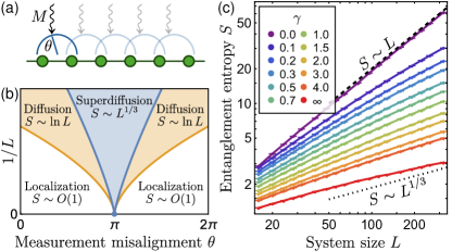
Figure 1: (a) Model: free-fermion chain of size $L$ monitored via frustrated measurements with a misalignment $\theta$. (b) “Phase diagram” of this system showing superdiffusion at $\theta=\pi$, with characteristic regimes of the entanglement scaling indicated by different colors. (c) Half-chain entanglement entropy $S$ as a function of $L$ for different values of the measurement strength $\gamma$ at fixed $\theta=\pi$. The dashed line shows the extensive (“ballistic”) behavior $S\sim L$, while the dotted line shows the fractal scaling $S\sim L^{1/3}$ corresponding to superdiffusion in 1+1-dimensional space-time.

In this Letter, we explore a 1D model of monitored free fermions, with the measurement operator being a particle number in a state residing on two adjacent sites (rather than on a single site), Fig. 1. This extension affects neither the U(1) symmetry (particle-number conservation) nor the local character of the measurement operator, nor the Gaussianity of the states. One could thus expect that the model belongs to the same “universality class” as previously studied 1D fermionic models [15]. Remarkably, this is not the case. We discover the emergence of the physics of superdiffusion (Lévy flights) of quantum information, with a fractal power-law scaling $S(\ell)\propto\ell^{1/3}$ in an intrinsically short-ranged model, which persists into the measurement-only limit.

Model.—We consider a model of monitored free fermions with non-commuting measurements and U(1) particle-number symmetry, on a periodic chain of $L$ sites (Fig. 1(a)). The monitored dynamics is characterized by the stochastic Schrödinger equation [4],

$$d\ket{\psi_{t+dt}} =\Big{[}-idtH-\frac{\gamma\,dt}{2}\sum_{i}(M_{i}-\langle M_{i}\rangle)^{2}$$

$$\quad+\sum_{i}d\xi_{i}^{t}(M_{i}-\langle M_{i}\rangle)\Big{]}\ket{\psi_{t}},$$ (1)

where $\gamma$ is the measurement strength, and $d\xi^{t}_{i}$ is the Itô increment with variance $\gamma\,dt$. The Hamiltonian includes fermion hopping, $H=J\sum_{i}c^{\dagger}_{i+1}c_{i}+\text{h.c.}$, where $J$ is the hopping strength. The measurement operator is a two-site projector

$$M_{i}=d_{i}^{\dagger}d_{i},\quad d_{i}=c_{i}\cos\frac{\theta}{4}+c_{i+1}\sin\frac{\theta}{4},$$ (2)

where parameter $\theta$ can be interpreted as a misalignment of the measurement apparatus that causes a superposition of two adjacent sites to be measured . When this misalignment is nonzero, the measurement operators on adjacent bonds do not commute, leading to frustration in the chain, with the maximal frustration happening for $\theta=\pi$. Since this evolution preserves the Gaussianity of the state, it is computationally simulable in polynomial time [4], and any state properties can be calculated from the corresponding single-particle correlation matrix ${\cal G}_{ij}=\braket{c_{i}^{\dagger}c_{j}}$.

Judging from the previous analytical description of monitored free fermions with the U(1) symmetry [15], one would be tempted to conclude that at a large enough spatial scale, this model should exhibit localization (i.e., area-law entanglement), with an intermediate logarithmic regime at small $\gamma$. However, a numerical analysis of the entanglement entropy at $\theta=\pi$ in Fig. 1(c) (where $\ell=L/2$) indicates the absence of localization, even at large measurement strengths. Furthermore, the data surprisingly reveal an entanglement growth that is faster than logarithmic: as we shall see later, in fact, the entropy grows as $S\sim\ell^{1/3}$, which corresponds to a superdiffusive transport in 1+1 (space-time) dimensions.

Effective field theory.— Our analytical description of the problem is based on the replicated Keldysh NLSM approach, developed in Refs. [15, 16, 24] and extended to weak measurements in Ref. [17], see Supplemental Material (SM) [37] for details. We introduce the Keldysh fermionic path-integral representation defined on $R\to 1$ replicas of the Keldysh contour. Averaging over the white noise $\xi(t)$ present in Eq. (Measurement-induced Lévy flights of quantum information) leads to the quartic fermionic term in the action. This term is decoupled by means of the Hubbard-Stratonovich matrix-valued field $\hat{Q}(x,t)$, which is interpreted as the local equal-time Green’s function of $d$-fermions, $Q_{\alpha\beta}(x,t)\sim 2\langle d_{\alpha}(x,t)d_{\beta}^{\ast}(x,t)\rangle$. Here, indices include the structure in the Keldysh and replica spaces, $\alpha,\beta\in\{+,-\}_{\text{K}}\otimes\{1,\dots,R\}_{\text{R}}$, and the spatial coordinate $x$ is a continuous version of the lattice index $i$. The Goldstone manifold consists of a replica-symmetric sector, the two-dimensional sphere $\mathrm{S}^{2}$, which describes the Lindbladian dynamics, and a replicon sector, the special unitary group $\hat{U}\in\mathrm{SU}(R)$, which describes the dynamics of observables that are non-linear in the density matrix. On this manifold, $\hat{Q}$ acquires the following block structure:

$$\hat{Q}=\begin{pmatrix}Q_{++}\hat{\mathbb{I}}&Q_{+-}\hat{U}\\ Q_{-+}\hat{U}^{\dagger}&Q_{--}\hat{\mathbb{I}}\end{pmatrix}_{\text{K}},$$ (3)

and satisfies the NLSM constraint ${\hat{Q}^{2}=\hat{\mathbb{I}}}$ along with ${\operatorname{Tr}\hat{Q}=0}$.

The crucial observation, which is responsible for the superdiffusive spreading of the quantum information in the system, is that the measurement-induced quasiparticle decay rate, obtained by means of the self-consistent Born approximation (SCBA), has the following momentum-dependent form:

$$\gamma_{k}=\gamma\left(1+\sin\frac{\theta}{2}\,\cos k\right),$$ (4)

and exactly vanishes at $k=\pm\pi$ for a special point $\theta=\pi$. Interestingly, this does not affect the diffusive behavior of the Lindbladian dynamics observed earlier [15] in the conventional density monitoring case $\theta=0$. The spatial diffusion coefficient consists of two contributions attributed to the unitary dynamics and non-commutativity of measurements,

$$D=\int_{-\pi}^{\pi}\frac{(dk)}{\gamma_{k}}\left[\left(\frac{\partial\xi_{k}}{\partial k}\right)^{2}+\frac{1}{4}\left(\frac{\partial\gamma_{k}}{\partial k}\right)^{2}\right]\\ =\frac{4J^{2}}{\gamma}\frac{1}{1+\left|\cos\frac{\theta}{2}\right|}+\frac{\gamma}{4}\left(1-\left|\cos\frac{\theta}{2}\right|\right),$$ (5)

and remains finite at $\theta=\pi$, since both the group velocity $\xi^{\prime}_{k}=-2J\sin k$ and the derivative $\gamma^{\prime}_{k}$ vanish at $k=\pm\pi$.

We now focus on the replicon sector, which describes observables of our interest, and parametrize $\hat{U}(x,t)$ via traceless Hermitian matrix field $\hat{\Phi}(x,t)$ as $\hat{U}=\exp(i\hat{\Phi})$. To see the emergence of superdiffusion, we inspect the quadratic form of the action (see SM [37] for the full action of NLSM). Vanishing of $\gamma_{k}$ leads to non-locality of the temporal term in the action:

$$S[\hat{\Phi}]=\frac{1}{4}\int dx\,\operatorname{Tr}\Bigg{\{}D\int_{-\infty}^{0}dt\,\left[\partial_{x}\hat{\Phi}(x,t)\right]^{2}\\ +\int_{-\infty}^{0}dt_{1}dt_{2}\,{\cal B}(t_{1}-t_{2})\,\partial_{t}\hat{\Phi}(x,t_{1})\partial_{t}\hat{\Phi}(x,t_{2})\Bigg{\}},$$ (6)

with the temporal diffusion coefficient ${\cal B}(\omega)$ [the Fourier transform of ${\cal B}(t)$] given by

$${\cal B}(\omega)=\int_{-\pi}^{\pi}\frac{(dk)}{\gamma_{k}-i\omega}=\frac{1}{\sqrt{(\gamma-i\omega)^{2}-\gamma^{2}\sin^{2}\frac{\theta}{2}}}\\ \stackrel{{\scriptstyle\omega\to 0}}{{\approx}}\begin{cases}\left(\gamma\left|\cos\frac{\theta}{2}\right|\right)^{-1},&\theta\neq\pi\,,\\ \left[-2i\gamma(\omega+i0)\right]^{-1/2},&\theta=\pi\,.\end{cases}$$ (7)

The emergence of superdiffusive Lévy flights with exponent $\alpha=3/2$—resulting in a heavy-tailed distribution of quantum-information spreading—in our NLSM theory at $\theta=\pi$ is manifest in the last line of Eq. (7).

The superdiffusive character of the field theory leads to the fractal scaling of observables. We focus below on the entanglement entropy (for a subsystem A of length $\ell$) $S_{A}=-\overline{\operatorname{Tr}\left(\hat{\rho}_{A}\ln\hat{\rho}_{A}\right)}$ and the charge correlation function

$$C(x-x^{\prime})=\overline{\left\langle\hat{n}(x)\hat{n}(x^{\prime})\right\rangle-\left\langle\hat{n}(x)\right\rangle\left\langle\hat{n}(x^{\prime})\right\rangle},$$ (8)

where the overbar denotes averaging over quantum trajectories. This correlation function determines the second cumulant of charge ${\cal C}_{A}^{(2)}$,

$${\cal C}_{A}^{(2)}=\overline{\left\langle\hat{N}_{A}^{2}\right\rangle-\left\langle\hat{N}_{A}\right\rangle^{2}}=\int_{0}^{\ell}\!dx\,dx^{\prime}\,C(x-x^{\prime}),$$ (9)

which, in view of the Gaussian character of the state, is related to the entropy via:

$$S_{A}\approx(\pi^{2}/3)\>{\cal C}_{A}^{(2)}.$$ (10)

The exact relation [38] contains also terms proportional to higher cumulants. However, they do not affect the scaling and amount to a small correction only, as was found for conventional density monitoring [15]; we have also verified this for the present model [37]. Both the entropy and the charge-cumulant generating function can be expressed via the NLSM partition function with appropriate boundary conditions [24, 37].

Fractality of correlations and entanglement.— We first consider the problem within the quasiclassical approximation with the Gaussian action (6). For $\delta=\theta-\pi\ll 1$, the Fourier transform of Eq. (8) reads

$$C(q)\approx\begin{cases}(2|\delta|)^{-1/2}|q\ell_{0}|&\text{for }q\ell_{0}\ll|\delta|^{3/2},\\ (2^{-2/3}3^{-1/2})|q\ell_{0}|^{2/3}&\text{for }q\ell_{0}\gg|\delta|^{3/2},\end{cases}$$ (11)

where $\ell_{0}=\sqrt{D/\gamma}\approx\sqrt{(2J/\gamma)^{2}+1/4}$ is the mean free path. Thus, $\delta=0$ ($\theta=\pi$) is a critical point, where $C(q)\propto q^{2/3}$ and the system exhibits a fractal (superdiffusive) scaling of the charge cumulant and entropy,

$$S_{A}\sim{\cal C}_{A}^{(2)}\sim\ell_{0}(L/\ell_{0})^{1/3}\quad\text{for}\ \ \ell=L/2\,,$$ (12)

explaining the surprising numerical results from Fig. 1. At small measurement strength $\gamma$, the entropy for small system sizes scales extensively with the system size $S\sim L$, which then experiences a ballistic-to-superdiffusion crossover as one increases $L$ or $\gamma$. This change in the entanglement behavior can be seen in Fig. 2, where we observe a nearly perfect data collapse of $S/\ell_{0}$ vs $L/\ell_{0}$ in a broad range of $\gamma$, from 0.1 to 4.0. Analytically, this universality of the crossover function is, strictly speaking, derived for $\gamma\ll 1$, in view of numerical corrections to the prefactor of $L^{1/3}$ scaling at $\gamma\gtrsim 1$, which come from spatial scales of the order of the level spacing and are not included in the NLSM analysis. We see, however, from Fig. 2 that the universality holds excellently up to a large measurement rate, $\gamma=4$. This universality shows that quantum corrections are essentially irrelevant even for large $\gamma$. A similar theory, with diffusive transport along one axis and superdiffusive along the other axis, was derived for transport in graphene with anisotropic disorder [39]. It was found there that quantum localization amounts to a finite correction only, without introducing strong localization or localization transition.

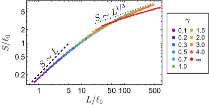
Figure 2: Collapse of $S/\ell_{0}$, where $S$ is half-chain entanglement entropy, as a function of $L/\ell_{0}$ for $\theta=\pi$ and different $\gamma$. The dashed line shows the ballistic behavior $S\sim L$, while the dotted line shows superdiffusion $S\sim L^{1/3}$.

Remarkably, the superdiffusive behavior and the absence of localization also hold in the measurement-only case, $\gamma=\infty$, in agreement with the analytical results. At the same time, the $\gamma=\infty$ data, when plotted as $S/\ell_{0}$ vs. $L/\ell_{0}$, deviate from the universal scaling curve. This has two reasons. First, for $\gamma=\infty$, corrections to the prefactor of the $L^{1/3}$ scaling mentioned in the preceding paragraph are particularly pronounced. Second, the $\gamma=\infty$ model belongs to a different symmetry class, as we are going to explain. A free-fermion system with particle-number conservation belongs to the BDI symmetry class when the Hamiltonian exhibits a particle-hole symmetry $H=-H^{T}$ and in the same basis the measurement operators are real $M=M^{*}$; otherwise, it belongs to the AIII class [20, 24]. For any finite $\gamma$, our model is therefore in the AIII class, while, for $\gamma=\infty$, the Hamiltonian is absent in the stochastic Schrödinger equation and the measurement-only point has a larger BDI symmetry. The difference between the NLSM field theories of these two classes is minimal and does not affect the qualitative behavior. The one-loop weak-localization correction in class BDI is negative and twice larger than that for class AIII. In our model, this is expected to lead to a numerical reduction of the prefactor of $S\sim L^{1/3}$ scaling in the $\gamma=\infty$ case (BDI class). This is what is observed in our simulations. We reiterate that the weak-localization correction in the present case is finite (i.e., not infrared divergent) and governed by short spatial scales.

For a non-zero (but small) $\delta$, the system exhibits a crossover from superdiffusive regime $C(q)\propto q^{2/3}$ to diffusive regime $C(q)\propto q$ at momentum $q\ell_{0}\sim|\delta|^{3/2}$, which corresponds to a lengthscale $\ell^{*}\sim\ell_{0}|\delta|^{-3/2}$. Ultimately, at large system sizes, the system then crosses over into localization, $C(q)/q\to 0$. We confirm this behavior using finite-size numerics in Fig. 3(a), where we plot the ratio $C(q)/q$. The three distinct regimes are clearly observed: superdiffusion (dashed line), diffusion (approximate saturation, with a slow decrease towards small $q$ due to weak-localization correction), and localization [vanishing $C(q)/q\propto q$ at $q\to 0$]. Translating to the real space, this implies that, as the system size is increased, one will first see the fractal (superdiffusive) entropy scaling $S\propto L^{1/3}$, then the logarithmic (diffusive) law $S\propto\ln L$, and finally the area law (localization) $S\simeq\text{const}$, see Fig. 1(b).

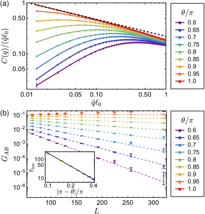
Figure 3: (a) Correlation function $C(q)$ as a function of rescaled momentum $\tilde{q}\ell_{0}$, where $\tilde{q}=2\sin(q/2)$ and $\ell_{0}=\sqrt{(2J/\gamma)^{2}+1/4}$, for $\gamma=4$ and different values of $\theta/\pi$. The system size used is $L=320$. The dashed line shows the superdiffusive behavior $C(q)/q\sim q^{-1/3}$. (b) Particle number covariance $G_{AB}$ as a function of system size $L$ for different values of $\theta/\pi$. Dashed lines are fits to $\sim\nobreak\exp(-L/4\ell_{\text{loc}})$ for $L\geq 128$. The extracted localization length is shown in the inset, along with a power-law fit $\ell_{\text{loc}}\sim|1-\theta/\pi|^{\nu}$, with exponent $\nu\approx 2.33(3)$ consistent with the analytical asymptotics (14) at numerically accessible scales.

In the diffusive regime, one can calculate the effective coupling constant (discarding localization effects),

$$\left.g=\frac{C(q)}{q}\right|_{\displaystyle q\ell^{*}\ll 1}\simeq\frac{\ell_{0}}{\sqrt{2}}|\delta|^{-1/2}.$$ (13)

This allows us to estimate the localization length, which scales at $|\delta|\ll 1$ as

$$\ell_{\text{loc}}\sim\ell^{*}\exp(4\pi g)\simeq\ell_{0}|\delta|^{-3/2}\exp\frac{2\sqrt{2}\pi\ell_{0}}{\sqrt{|\delta|}}.$$ (14)

The localization length $\ell_{\text{loc}}(\delta)$ thus diverges exponentially at the critical point $\delta=0$. If one fits Eq. (14) to a power-law form $\ell_{\text{loc}}\sim|\delta|^{-\nu}$ in a restricted range of $\delta$, one will get an “effective exponent” $\nu$ that increases from 3/2 towards infinity when one approaches the singular point $\delta=0$.

To probe the localization in real space numerically, we use the particle-number covariance, $G_{AB}=\overline{\langle N_{A}\rangle\langle N_{B}\rangle-\langle N_{A}N_{B}\rangle}$, where $N_{A}$ and $N_{B}$ are particle-number operators of antipodal regions $A$ and $B$, each of size $L/4$. This observable yields an effective conductance at scale $\sim L/4$ and scales in the area-law phase asymptotically as $G_{AB}\sim\exp(-L/4\ell_{\text{loc}})$. Numerical results for $G_{AB}(L)$ shown in Fig. 3(b) confirm that localization sets in when $\theta\neq\pi$. By fitting $G_{AB}(L)$ to the exponential law for $L\geq 128$ (dashed lines), we obtain estimates for the localization length $\ell_{\rm loc}(\delta)$ shown in the inset. The results clearly support the analytically predicted divergence of $\ell_{\rm loc}$ at $\delta\to 0$. Accurately verifying Eq. (14) in this way is hardly possible since $\ell_{\rm loc}$ quickly becomes very large at small $\delta$, where this formula holds. Instead, we show in the inset a power-law fit $\ell_{\text{loc}}\sim|\delta|^{-\nu}$, which yields effective exponent $\nu\approx 2.33(3)$, which is larger than 3/2 in agreement with a discussion below Eq. (14). Note that this effective exponent is not too far from 3/2, which reflects the difficulty in numerical verification of the exponential dependence in Eq. (14): when the exponential decay of $G_{AB}(L)$ is observed for realistic system sizes, the localization length is only a few times larger than $\ell^{*}\sim\ell_{0}|\delta|^{-3/2}$.

Discussion and outlook.— Summarizing, the free-fermion model with two-site monitoring operators (2) is characterized, at $\theta=\pi$, by a superdiffusive NLSM, which leads to the fractal scaling of the entanglement entropy, $S\propto L^{1/3}$, and charge correlations, $C(q)\propto q^{2/3}$. When $\theta$ deviates from the critical point $\pi$, the superdiffusive scaling is transient, giving rise to diffusion and, eventually, localization at longer length scales (smaller $q$). The superdiffusive behavior originates from the vanishing of the measurement-induced quasiparticle decay rate $\gamma_{k}$ at one point in the Brillouin zone and should also hold for other models of monitoring having this property (also for other symmetry classes). An example is a model with measurement of conventional site density $c_{i}^{\dagger}c_{i}$ but on even sites only. A related mechanism of Lévy flights was found to be operative in non-monitored models with “nodal” disorder [39, 40], dephasing [41], and interactions [42]. Our discovery of measurement-induced Lévy flights opens up avenues for the study of exotic entangled phases and novel quantum-information transport mechanisms.

Acknowledgments.— A. P. and M. S. were funded by the European Research Council (ERC) under the European Union’s Horizon 2020 research and innovation programme (Grant Agreement No. 853368). C. J. T. is supported by an EPSRC fellowship (Grant Ref. EP/W005743/1). The authors acknowledge the use of the UCL High Performance Computing Facilities (Myriad), and associated support services, in the completion of this work.

Supplemental Material to “Measurement-induced Lévy flights of quantum information”

S1 Derivation of superdiffusive NLSM

Here, we derive the effective action of the NLSM field theory for the measurement protocol considered in the present Letter. The derivation is based on the approach developed in Refs. [15, 16, 24]. The crucial difference is that now we monitor the density of $d$-fermions, which are linearly related to the original fermions $c$. An additional difference is that the present protocol corresponds to continuous monitoring, as opposed to projective measurements studied in Refs. [15, 16]; this, however, does not qualitatively affect the results.

Fermionic action for weak measurements

Continuous measurements of an arbitrary operator $\hat{M}$ can be realized via a complete set of Kraus operators enumerated with an index $\alpha\in\mathbb{R}$ corresponding to possible measurement outcomes:

$$\hat{\mathbb{K}}_{\alpha}=\exp\left[-\gamma dt\left(\hat{M}-\alpha\right)^{2}\right],\qquad\sqrt{\frac{2\gamma dt}{\pi}}\int_{-\infty}^{+\infty}d\alpha\,\hat{\mathbb{K}}_{\alpha}^{\dagger}\hat{\mathbb{K}}_{\alpha}=\hat{\mathbb{I}}$$ (S1)

Following Ref. [24], we introduce a replicated fermionic Keldysh path integral representation, and first focus on each individual replica and a given “measurement trajectory”—that is, a realization of measurement outcomes $\{\alpha_{m}\}$, where $m$ enumerates discrete time steps. The Lagrangian consists of a replica-diagonal contribution describing the unitary evolution:

$${\cal L}_{0}[c]=c^{\dagger}\left(i\partial_{t}-\hat{H}_{0}\right)c,\qquad c\equiv\begin{pmatrix}c_{+}\\ c_{-}\end{pmatrix}_{\text{K}},\qquad c^{\dagger}\equiv\begin{pmatrix}c_{+}^{\ast}&-c_{-}^{\ast}\end{pmatrix}_{\text{K}},$$ (S2)

and a measurement-induced contribution that acquires the following form:

$$\prod_{m}\mathbb{K}_{\alpha_{m}}^{(+)}(t_{m})\mathbb{K}_{\alpha_{m}}^{(-)}(t_{m})\simeq\exp\left[i\int dt\,{\cal L}_{M}(\xi(t))\right],\qquad i{\cal L}_{M}(\xi)=-\gamma\sum_{s=\pm}\left(\frac{\xi(t)}{2\gamma}-M_{s}(t)+\frac{1}{2}\right)^{2},$$ (S3)

where continuous (in the limit $dt\to 0$) field $\xi(t_{m})\equiv\gamma(2\alpha_{m}-1)$ is introduced.

For the case of density monitoring, $\hat{M}=\hat{d}^{\dagger}\hat{d}$, where $\hat{d}$ is an arbitrary (different from $\hat{c}$) set of fermions, we employ the “principal value” regularization procedure described in detail in Ref. [15] and arrive at the “symmetrized” coherent state representation $M(d^{\ast},d)=1/2+d^{\ast}d$. Utilizing the Grassmann nature of fields $d$, we finally arrive at the following Lagrangian:

$$i{\cal L}_{M}(\xi,d)=-\frac{\xi^{2}}{2\gamma}+\xi\,d^{\dagger}\hat{\tau}_{z}d,$$ (S4)

where $\hat{\tau}_{\alpha}$ are the Pauli matrices acting in the Keldysh space.

The full replicated action for the problem considered in the present Letter is then easily obtained by (i) introducing additional index $i$ enumerating the measurement operators (i.e. lattice sites), and performing summation over them, and (ii) performing summation over $R$ replicas, with the replica limit $R\to 1$ following from the Born’s rule. Thus, the effect of weak measurements of fermionic density is described, within this replicated theory, by introducing a Gaussian white-noise field $\xi_{i}(t)$ with the correlation function $\left\langle\xi_{i}(t)\xi_{j}(t^{\prime})\right\rangle=(\gamma/R)\delta_{ij}\delta(t-t^{\prime})$ and coupling this noise to $d^{\dagger}\hat{\tau}_{z}d$ on the Keldysh contour. Finally, Gaussian integration over $\xi_{i}(t)$ yields a quartic “interaction”, so that the full Lagrangian reads:

$$i{\cal L}=ic^{\dagger}\left(i\partial_{t}-\hat{H}_{0}\right)c+\frac{\gamma}{2R}\left(d^{\dagger}\hat{\tau}_{z}d\right)^{2}\,.$$ (S5)

Here, the (time- and space-dependent) fields $c$ and $d$ “live” in the $R$-dimensional replica space and, in addition, in the two-dimensional Keldysh space.

Effective matrix field theory

We perform the Hubbard-Stratonovich transformation to decouple the quartic term simultaneously in two possible channels, following the procedure from Ref. [15]. First, we introduce an auxiliary matrix field $\hat{{\cal G}}$ via the functional delta-function $\delta_{\text{slow}}[\mathcal{F}]$, which, however, fixes only the “slow” components (introducing a momentum cutoff). We represent this delta-function through an auxiliary integral by introducing matrix field $\hat{\tau}_{z}\hat{Q}$:

$$1=\int{\cal D}{\cal G}\,\delta_{\text{slow}}\!\left[{\cal G}-dd^{\dagger}\tau_{z}\right]=\int{\cal D}{\cal G}{\cal D}Q\,\exp\left[-\frac{\gamma}{2R}\operatorname{Tr}\left(\hat{{\cal G}}\hat{\tau}_{z}\hat{Q}\right)-\frac{\gamma}{2R}d^{\dagger}\hat{Q}d\right].$$ (S6)

Next, we decouple the quartic term in two channels, utilizing the delta function; such a procedure is equivalent to applying Wick’s theorem to the corresponding term (cf. Ref. [15]):

$$\left(d^{\dagger}\hat{\tau}_{z}d\right)^{2}\simeq-\operatorname{Tr}\hat{{\cal G}}^{2}+\operatorname{Tr}^{2}\hat{{\cal G}}.$$ (S7)

We then perform Gaussian integration over $\hat{{\cal G}}$, arriving at:

$$\int{\cal D}{\cal G}\,\exp\left\{-\frac{\gamma}{2R}\left[\operatorname{Tr}\left(\hat{{\cal G}}^{2}+\hat{{\cal G}}\hat{\tau}_{z}\hat{Q}\right)-\operatorname{Tr}^{2}\hat{{\cal G}}\right]\right\}=\exp\left\{\frac{\gamma}{8R}\left[\operatorname{Tr}(\hat{\tau}_{z}\hat{Q})^{2}-\frac{1}{2R-1}\operatorname{Tr}^{2}(\hat{\tau}_{z}\hat{Q}_{0})\right]\right\}.$$ (S8)

As the final step, we note that for the problem we consider in this Letter, fermions $d$ and $c$ obey a linear relation with an auxiliary matrix $\hat{m}$

$$d=\hat{m}c,\quad m_{i,i}=\cos\frac{\theta}{4},\quad m_{i,i+1}=\sin\frac{\theta}{4}.$$ (S9)

Utilizing this relation and performing Gaussian integration over fermions $c$, we finally arrive at the following effective action for the “slow” matrix field $\hat{Q}$:

$$-S[\hat{Q}]=\operatorname{Tr}\ln\left(i\partial_{t}-\hat{H}_{0}+\frac{i\gamma}{2R}\hat{m}^{\dagger}\hat{Q}\hat{m}\right)+\frac{\gamma}{8R}\left\{\operatorname{Tr}\left[\left(\tau_{z}\hat{Q}\right)^{2}\right]-\frac{1}{2R-1}\operatorname{Tr}^{2}\left(\hat{\tau}_{z}\hat{Q}\right)\right\}.$$ (S10)

Self-consistent Born approximation and saddle-point manifold

First, we put $R=1$ and focus on the replica-symmetric sector. As in earlier works, we note that for arbitrary $2\times 2$ matrix $\hat{Q}_{0}$, there is an exact identity:

$$\operatorname{Tr}\left[\left(\hat{\tau}_{z}\hat{Q}_{0}\right)^{2}\right]-\operatorname{Tr}^{2}\left(\hat{\tau}_{z}\hat{Q}_{0}\right)\equiv\operatorname{Tr}^{2}\hat{Q}_{0}-\operatorname{Tr}\left(\hat{Q}_{0}^{2}\right),$$ (S11)

which implies that arbitrary unitary rotations $\hat{Q}_{0}\mapsto\hat{{\cal R}}\hat{Q}_{0}\hat{{\cal R}}^{-1}$ form a symmetry group of the action given by Eq. (S10). The saddle-point equation (for a traceless matrix $\operatorname{Tr}\hat{Q}_{0}=0$) then yields:

$$\hat{Q}_{0}(\boldsymbol{r})=2i\left(\hat{m}\hat{G}_{Q_{0}}\hat{m}^{\dagger}\right)_{\boldsymbol{r}\boldsymbol{r}},\quad\text{where}\quad\hat{G}_{Q}=\left(i\partial_{t}-\hat{H}_{0}+i\frac{\gamma}{2}m^{\dagger}\hat{Q}\hat{m}\right)^{-1},$$ (S12)

where $\boldsymbol{r}=(x,t)$ is the space-time coordinate. When we look for a homogeneous solution, $\hat{Q}_{0}(\boldsymbol{r})=\hat{Q}_{0}=\operatorname{const}$, this equation reduces to

$$\hat{Q}_{0}=2i\int\frac{(d\varepsilon)(dk)|m_{k}|^{2}}{\varepsilon-\xi_{k}+i\gamma_{k}\hat{Q}_{0}/2}\qquad\Longrightarrow\qquad\hat{Q}_{0}=\operatorname{sign}\hat{Q}_{0}\,,$$ (S13)

where we have introduced Fourier transform $m_{k}$ of matrix $\hat{m}$ and momentum-dependent decay rate $\gamma_{k}$ [given by Eq. (4) of the main text]:

$$m_{k}=\cos\frac{\theta}{4}+e^{ik}\sin\frac{\theta}{4},\quad\gamma_{k}\equiv\gamma|m_{k}|^{2}=\gamma\left(1+\sin\frac{\theta}{2}\,\cos k\right).$$ (S14)

Thus, an arbitrary matrix satisfying $\hat{Q}_{0}^{2}=\hat{\mathbb{I}}$ and $\operatorname{Tr}\hat{Q}_{0}=0$ provides a solution. This yields the saddle-point manifold of the replica-symmetric sector of the theory, which is the two-dimensional sphere $\mathrm{S}^{2}$. On this manifold, there is a special point (SCBA solution)

$$\hat{Q}_{\text{SCBA}}=\hat{\Lambda}=\begin{pmatrix}1-2n_{0}&2n_{0}\\ 2(1-n_{0})&-(1-2n_{0})\end{pmatrix}_{\text{K}},$$ (S15)

which yields the average value of the Green function, as determined by causality. Here $n_{0}$ is the filling factor of the band, which is conserved and thus determined by initial conditions. (Formally, $n_{0}=\left\langle\hat{d}_{i}^{\dagger}\hat{d}_{i}\right\rangle_{0}$, but average density for fermions $\hat{d}$ is same as for fermions $\hat{c}$.) The replica-symmetric manifold $\mathrm{S}^{2}$ is obtained by rotations of $\Lambda$ in Keldysh space. The full saddle-point manifold in the $R\to 1$ limit is then obtained by noting that, for $R\neq 1$, arbitrary rotations that commute with $\hat{\tau}_{z}$ also produce a symmetry, yielding the structure given by Eq. (3) of the main text.

Gradient expansion

We substitute $\hat{Q}=\hat{{\cal R}}\hat{\Lambda}\hat{{\cal R}}^{-1}$ in the action (S10) and identically rewrite the trace-log term in a form suitable for gradient expansion:

$$-S[\hat{Q}]=\operatorname{Tr}\ln\left(1+\hat{G}_{\Lambda}\hat{{\cal R}}^{-1}\left[i\partial_{t}-\hat{H}_{0},\hat{{\cal R}}\right]+\frac{i\gamma}{2}\hat{G}_{\Lambda}\left(\hat{{\cal R}}^{-1}\hat{m}^{\dagger}\hat{{\cal R}}\hat{\Lambda}\hat{{\cal R}}^{-1}\hat{m}\hat{{\cal R}}-\hat{m}^{\dagger}\hat{\Lambda}\hat{m}\right)\right),$$ (S16)

where $\hat{G}_{\Lambda}$ is given by $\hat{G}_{Q}$ from Eq. (S12) with $\hat{Q}\to\hat{\Lambda}$, matrices $\hat{m}$ are introduced in Eq. (S9), and the limit $R\to 1$ was taken.

The first order of the expansion of Eq. (S16) yields two terms. The first term is the standard Wess-Zumino term, contributing to the replica-symmetric sector only and governing its time dynamics:

$$-S_{t}^{(1)}[\hat{Q}]=\frac{1}{2}\operatorname{Tr}\left(\hat{\Lambda}\hat{{\cal R}}^{-1}\partial_{t}\hat{{\cal R}}\right).$$ (S17)

The second term arises due to the non-commutativity of measurements and gives a contribution to the diffusion coefficient:

$$-S_{x}^{(1)}[\hat{Q}]=\frac{\gamma}{8}\operatorname{Tr}\left(\left[\hat{m}^{\dagger},\hat{Q}\right]\left[\hat{m},\hat{Q}\right]\right)\approx-\frac{D_{1}}{8}\operatorname{Tr}\left(\partial_{x}\hat{Q}\right)^{2},\quad D_{1}=-\gamma\operatorname{Tr}\left(\left[\hat{m}^{\dagger},\hat{x}\right]\left[\hat{m},\hat{x}\right]\right).$$ (S18)

Yet another contribution to the diffusion coefficient arises from the second-order expansion in a standard way, and yields:

$$-S_{x}^{(2)}[\hat{Q}]=-\frac{1}{4}\operatorname{Tr}\Bigg{[}\hat{G}_{R}\left(1+\hat{\Lambda}\right)\hat{{\cal R}}^{-1}\partial_{x}\hat{{\cal R}}\left(\left[\hat{H}_{0},\hat{x}\right]-\frac{i\gamma}{2}\left(\hat{m}^{\dagger}\left[\hat{m},\hat{x}\right]-\left[\hat{m}^{\dagger},\hat{x}\right]\hat{m}\right)\right)\\ \times\hat{G}_{A}(1-\hat{\Lambda})\hat{{\cal R}}^{-1}\partial_{x}\hat{{\cal R}}\left(\left[\hat{H}_{0},\hat{x}\right]+\frac{i\gamma}{2}\left(\hat{m}^{\dagger}\left[\hat{m},\hat{x}\right]-\left[\hat{m}^{\dagger},\hat{x}\right]\hat{m}\right)\right)\Bigg{]}\approx-\frac{D_{2}}{8}\operatorname{Tr}(\partial_{x}\hat{Q})^{2},$$ (S19)

where

$$D_{2}=\int(dk)\left\{\frac{1}{\gamma_{k}}\left[\left(\partial_{k}\xi_{k}\right)^{2}+\frac{1}{4}\left(\partial_{k}\gamma_{k}\right)^{2}\right]-\gamma|\partial_{k}m_{k}|^{2}\right\},$$ (S20)

and

$$G_{R/A}(\varepsilon,k)=\frac{1}{\varepsilon-\xi_{k}\pm i\gamma_{k}/2}.$$ (S21)

The full diffusion coefficient $D=D_{1}+D_{2}$ is then given by Eq. (5) of the main text. Due to the non-locality of matrix $\hat{m}$, the diffusion coefficient $D$ is nonzero even in the measurement-only limit $J=0$.

Finally, we focus on the term that governs the time dynamics of the replicon sector and is responsible for the Lévy flights. This term arises from the expansion beyond the first order with respect to the temporal-gradient term. It is sufficient to neglect the spatial dependence of $\hat{Q}$-matrix and focus on the temporal dependence only. Furthermore, we neglect fluctuations of the replica-symmetric sector here and make the following substitution:

$$\hat{{\cal R}}=\begin{pmatrix}\hat{{\cal V}}_{+}&0\\ 0&\hat{{\cal V}}_{-}\end{pmatrix}\ \Rightarrow\ \hat{{\cal R}}^{-1}i\partial_{t}\hat{{\cal R}}=\begin{pmatrix}i\hat{{\cal V}}_{+}^{-1}\partial_{t}\hat{{\cal V}}_{+}&0\\ 0&i\hat{{\cal V}}_{-}^{-1}\partial_{t}\hat{{\cal V}}_{-}\end{pmatrix},$$ (S22)

with ${\cal V}_{\pm}\in\mathrm{SU}(R)$ and $\hat{U}=\hat{{\cal V}}_{+}\hat{{\cal V}}_{-}^{\dagger}$. The corresponding contribution to the action then reads:

$$S_{t}[Q]\approx-\int dx\int(dk)\operatorname{Tr}\ln\left(1+\hat{G}_{\Lambda}(k)\hat{{\cal R}}^{-1}(x,t)i\partial_{t}\hat{{\cal R}}(x,t)\right).$$ (S23)

Expanding this term to the second order, we obtain:

$$S_{t}^{(2)}[\hat{Q}]=n_{0}(1-n_{0})\int dxdt_{1}dt_{2}{\cal B}(t_{1}-t_{2})\operatorname{Tr}\left[\hat{{\cal J}}_{t}(x,t_{1})\hat{{\cal J}}_{t}(x,t_{2})\right],$$ (S24)

where the diffuson ladder block $\mathcal{B}$ is defined as

$${\cal B}(\omega)=\int(dk)(d\varepsilon)G_{R}\left(\varepsilon+\frac{\omega}{2},k\right)G_{A}\left(\varepsilon-\frac{\omega}{2},k\right),$$ (S25)

which yields Eq. (7) of the main text. Further, the “current” $\hat{{\cal J}}_{t}$ in Eq. (S24) is defined as

$$\hat{{\cal J}}_{t}=\hat{{\cal J}}_{t}^{(+)}-\hat{{\cal J}}_{t}^{(-)},\quad\text{with}\quad\hat{{\cal J}}_{t}^{(\pm)}=i\hat{{\cal V}}_{\pm}^{\dagger}\partial_{t}\hat{{\cal V}}_{\pm}$$ (S26)

For maximal misalignment of the measurements, $\theta=\pi$, we have ${\cal B}(\omega)\propto\omega^{-1/2}$, see Eq. (7), and thus ${\cal B}(t)\propto t^{-1/2}$ for the kernel in Eq. (S24). We have thus a NLSM effective theory with a long-range coupling decaying as a power law. This non-locality of the NLSM action implies the emergence of superdiffusive Lévy flights. If one expands the matrix $\hat{U}$ with respect to its deviations from the saddle point $\hat{\mathbb{I}}$, i.e., $\hat{U}=\exp(i\hat{\Phi})\approx\hat{\mathbb{I}}+i\hat{\Phi}$ with $\Phi\ll 1$, then the lowest-order terms in Eq. (S24) give the action (6) of the main text. This action yields the following propagator in the “bulk” (i.e., sufficiently far from the boundary in the time domain):

$$\left\langle\Phi_{ab}(\omega,q)\Phi_{cd}(-\omega,-q)\right\rangle=\left(\delta_{ad}\delta_{bc}-\frac{1}{R}\delta_{ab}\delta_{cd}\right)\mathcal{D}_{\Phi}(\omega,q),$$ (S27)

where the replica structure originates from tracelessness of generator $\hat{\Phi}$, and, for the half-filling case $n_{0}=1/2$:

$$\mathcal{D}_{\Phi}(\omega,q)=\frac{2}{\omega^{2}\operatorname{Re}{\cal B}(\omega)+Dq^{2}}\underset{\omega,q\to 0}{\approx}\begin{cases}\displaystyle\frac{2}{\omega^{2}/\gamma|\cos\frac{\theta}{2}|+Dq^{2}},&\theta\neq\pi\,;\\[14.22636pt] \displaystyle\frac{2}{|\omega|^{3/2}/2\gamma^{1/2}+Dq^{2}},&\theta=\pi\,.\end{cases}$$ (S28)

The following subtle point should be mentioned here. The non-local Eq. (S24) is, strictly speaking, not gauge-invariant, even though it was obtained from the expansion of the manifestly gauge-invariant trace-log term. Indeed, a gauge transformation $\hat{{\cal V}}_{\pm}\mapsto\hat{{\cal V}}_{\pm}\hat{{\cal V}}$, which leaves matrix $\hat{U}$ unchanged, affects the current as $\hat{{\cal J}}_{t}\mapsto i\hat{{\cal V}}^{\dagger}\hat{{\cal J}}_{t}\hat{{\cal V}}$. In the conventional “diffusive” case ($\theta$ far from $\pi$ in our model), when ${\cal B}(t)$ can be replaced by the delta-function [i.e., $\mathcal{B}(\omega\to 0)$ is finite], the second order in the expansion of the trace-log acquires the following, gauge invariant, form:

$$S_{t}^{(2)}[\hat{Q}]\approx n_{0}(1-n_{0}){\cal B}(\omega=0)\int dxdt\operatorname{Tr}\left[\partial_{t}\hat{U}^{\dagger}\partial_{t}\hat{U}\right],$$ (S29)

characteristic of a diffusive NLSM. In this case, higher-order terms of the expansion contain additional smallness in $\omega/\gamma\ll 1$. On the other hand, in the case of the super-diffusion, with $\mathcal{B}(\omega\to 0)$ having a power-law divergence, a careful analysis reveals that higher-order terms do not contain such smallness and whole series has to be resummed in order to restore strict gauge invariance. These higher-order corrections to Eq. (S24) have the structure

$$S_{t}^{(k)}[\hat{Q}]\sim\sum_{s_{i}=\pm}\int dxdt_{1}\ldots dt_{k}{\cal B}_{s_{1}\dots s_{k}}^{(k)}(t_{1}-t_{2},\ldots,t_{1}-t_{k})\operatorname{Tr}\left[\hat{{\cal J}}_{t}^{(s_{1})}(x,t_{1})\ldots\hat{{\cal J}}_{t}^{(s_{k})}(x,t_{k})\right],\qquad k=3,4,\ldots\,,$$ (S30)

where the kernels ${\cal B}_{s_{1}\dots s_{k}}^{(k)}$ are homogeneous functions of fractional degree $-1/2$. When one expands in $\hat{\Phi}$ to the order $k$, only first $k$ terms in the series contribute, and their sum is gauge-invariant. In particular, to the Gaussian order, only the $k=2$ term (S24) contributes, giving Eq. (6) of the main text, as explained above.

For weak monitoring (small $\gamma$), the Gaussian approximation, Eq. (6) of the main text, fully determines the density correlation function of the NLSM theory, with quantum corrections originating from higher terms being negligibly small. At the same time, one can ask whether quantum effects may lead to strong localization in the limit of large $\gamma$. If this would be the case, we would have a localization transition at some intermediate $\gamma$. A rigorous analytic answer to this question requires a careful renormalization-group analysis of our NLSM theory. We leave this for the future, providing here the following arguments. Renormalization-group analysis of NLSM theories with power-law couplings was performed in Ref. [45] for a matrix NLSM, see also the early paper on a vector NLSM [46]. It was found in these works that, in the replica limit (in which the number of degrees of freedom is zero) and for sufficiently slowly decaying couplings, there is no infrared quantum corrections. As a consequence, there is no transition: the behavior of the correlation functions is the same as in the Gaussian (quasiclassical) approximation. In fact, our NLSM is different in several aspects from those studied in Refs. [45, 46]: (i) it is of a different symmetry class, (ii) its action includes a series of terms (S30), (iii) the action is superdiffusive with respect to $t$ direction but conventional diffusive in $x$ direction. We expect, however, that these differences do not affect the conclusion about the absence of transition. An additional argument supporting this is the result of Ref. [39] where a similar theory (diffusion in one direction and superdiffusive in another direction) was obtained for a problem of transport in a 2D disordered system with a special type of disorder. It was found in Ref. [39] from the inspection of a weak-localization correction (and supported by numerics there) that there are only finite quantum corrections but no localization transition.

We thus argue that the superdiffusive behavior (at $\theta=\pi$) obtained from the Gaussian approximation to our NLSM holds also for large $\gamma$, and there is no localization transition in this model. This is supported also by our numerical results shown in the main text of the paper.

Boundary conditions

Finally, we relate the derived NLSM field theory to observable quantities [24]. The theory is defined on the semi-axis $t<0$ in the time domain, whereas at $t=0$ one has to introduce boundary conditions. We define the partition function with arbitrary boundary conditions as follows:

$$Z_{A}[\hat{U}_{0}]=\int{\cal D}\hat{U}\,\exp\left(-S[\hat{U}]\right),\quad\text{subject to}\quad\begin{cases}\hat{U}(x\in A,t=0)=\hat{U}_{0}\oplus\hat{\mathbb{I}}_{R-N}\\ \hat{U}(x\notin A,t=0)=\hat{\mathbb{I}}_{R}\end{cases},$$ (S31)

where the matrix $\hat{U}_{0}$ has a size $N\times N$ with $N\leq R$.

Both the entanglement entropy and the charge generating function for arbitrary region $A$ can be then expressed via such partition function as follows:

$$S_{A} \equiv-\overline{\operatorname{Tr}\left(\hat{\rho}_{A}\ln\hat{\rho}_{A}\right)}=-\lim_{N\to 1}\frac{\ln Z[\hat{\mathbb{T}}_{N}]}{N-1},$$ (S32)

$$\chi_{A}(\lambda) \equiv\overline{\ln\left\langle e^{i\lambda\left(\hat{N}_{A}-\left\langle\hat{N}_{A}\right\rangle\right)}\right\rangle}=\lim_{N\to 1}\frac{\ln Z[e^{i\hat{\lambda}_{N}}]}{N-1},$$ (S33)

which involve auxiliary matrices of the following structure (shown here for $N=3$):

$$\hat{\mathbb{T}}_{N}=\begin{pmatrix}0&-1&0\\ 0&0&-1\\ 1&0&0\end{pmatrix},\quad e^{i\hat{\lambda}}=\begin{pmatrix}e^{i\lambda}&0&0\\ 0&e^{i\lambda}&0\\ 0&0&e^{-i(N-1)\lambda}\end{pmatrix}.$$ (S34)

Formally, such a procedure determines the fluctuation of charge of fermions $d$, as well as entanglement entropy calculated in the basis of fermions $d$ rather than original fermions $c$. However, since the relation between $c$-fermions and $d$-fermions is local (involves two adjacent sites only) and we are interested in the behavior for a large size of the region $A$, this difference is not essential since it may only give corrections proportional to the surface area of the region $A$, i.e. $\sim O(\partial A)$, i.e., a constant of order unity for 1D systems studied here.

The entanglement entropy can be alternatively expressed through the statistics of fluctuations of charge via the Klich-Levitov relation:

$$\chi_{A}(\lambda)\equiv\sum_{n=0}^{\infty}\frac{(i\lambda)^{n}}{n!}{\cal C}_{A}^{(n)}\quad\Longrightarrow\quad S_{A}=\sum_{n=1}^{\infty}2\zeta(2n){\cal C}_{A}^{(2n)},$$ (S35)

where ${\cal C}_{A}^{(n)}$ is the $n$-th cumulant of charge.

The quadratic expansion (6) allows us to calculate only the second cumulant ${\cal C}_{A}^{(2)}$, or, equivalently, the pair density correlation function $C(x-y)$ in the Gaussian approximation controlled by a large value of the “dimensionless conductance” (inverse of which controls the magnitude of quantum corrections). However, we have seen earlier [15, 16] for a model with conventional density monitoring, the second cumulant is sufficient to determine the entanglement entropy with very good precision in all regimes. We have checked numerically that this holds also for the present model. In Fig. S1, the ratio of the entanglement entropy to the second cumulant, $S/\mathcal{C}^{(2)}$, in our superdiffusive model ($\theta=\pi$) is shown for various system sizes and various monitoring strength. It is seen that this ratio is very close (within a few percent) to $2\zeta(2)=\pi^{2}/3$, i.e., Eq. (10) of the main text holds with excellent accuracy.

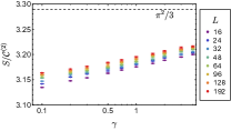
Figure S1: Numerical results for the ratio $S/\mathcal{C}^{(2)}$ for a subsystem of length $L/2$ at $\theta=\pi$, for various monitoring strength $\lambda$ and system size $L$. The dashed line shows the value of $\pi^{2}/3$.

S2 Saddle point approximation:  Density correlation function and second charge cumulant

Action

In this Section of the Supplemental Material, we calculate the density-density correlation function $C(q)$ and charge fluctuations ${\cal C}_{A}^{(2)}$ in the saddle-point approximation. This requires finding the minima of action (6) subject to the following boundary conditions:

$$\hat{\Phi}(x,t=0)=\begin{pmatrix}\lambda(x)&0&0\\ 0&\lambda(x)&0\\ 0&0&-(N-1)\lambda(x)\end{pmatrix},$$ (S36)

which follow from Eqs. (S31,S33,S34), and where we have kept the density source $\lambda(x)$ arbitrary. The charge fluctuations in the given region $A$ correspond to the specific choice $\lambda(x\in A)=\lambda$ and zero otherwise. Given the diagonal form of boundary conditions, the solution for the saddle-point equations can also be sought in the diagonal form:

$$\hat{\Phi}(x,t)=\varphi(x,t)\cdot\begin{pmatrix}1&0&0\\ 0&1&0\\ 0&0&-(N-1)\end{pmatrix},$$ (S37)

with the scalar function $\varphi(x,t)$. The action (6) with this Ansatz reduces to

$$S[\hat{\Phi}]=N(N-1)S_{0}[\varphi].$$ (S38)

The generating function (S33) in the saddle-point approximation then yields $\chi[\lambda]=-S_{0}[\varphi]$, with the action calculated on the saddle-point solution.

With the suitable choice of units of time, the action $S_{0}$ can be brought to the following form:

$$S_{0}[\varphi]=\frac{g_{0}}{2}\int dx\left[\int_{-\infty}^{0}dt\,\big{(}\partial_{x}\varphi(x,t)\big{)}^{2}+\int_{-\infty}^{0}dt_{1}\int_{-\infty}^{0}dt_{2}\,L(t_{1}-t_{2})\,\partial_{t}\varphi(x,t_{1})\partial_{t}\varphi(x,t_{2})\right],\quad L(\omega)=|\omega|^{\alpha-2},$$ (S39)

subject to the boundary conditions $\varphi(x,t=0)=\lambda(x)$. Here, $\alpha=2$ corresponds to standard diffusion and $\alpha=3/2$ corresponds to the model under consideration. The constant $g_{0}$ will be specified below. In the present calculation, we will consider arbitrary $\alpha\in(1,2]$.

Wiener-Hopf problem

We perform a spatial Fourier transformation and seek for the solution in the form:

$$\varphi_{q}(t)=\lambda_{q}\psi\left(\tau\equiv q^{2/\alpha}t\right),$$ (S40)

with a single dimensionless function $\psi(\tau)$; the saddle-point equation is then equivalent to

$$\psi(\tau)-\frac{\partial^{2}}{\partial\tau^{2}}\int_{-\infty}^{0}d\tau^{\prime}L(\tau-\tau^{\prime})\psi(\tau^{\prime})=\frac{\partial L(\tau)}{\partial\tau},\quad\psi(0)=1.$$ (S41)

The action calculated on such a saddle-point configuration reads:

$$S_{0}[\varphi]=\frac{1}{2}\int(dq)C(q)\lambda_{q}\lambda_{-q},\quad C(q)=c_{0}g_{0}|q|^{2\left(1-1/\alpha\right)},\quad c_{0}=\int_{-\infty}^{0}d\tau\psi(\tau).$$ (S42)

This form of the saddle point action then implies that the function $C(q)$ then identically yields the correlation function of densities.

To solve Eq. (S41), we employ the Wiener-Hopf method. We continue this equation to the entire line $\tau\in\mathbb{R}$ and seek the solution in the form

$$\psi(\tau)=\psi_{+}(\tau)+\psi_{-}(\tau),$$

where $\psi_{+}(\tau<0)=\psi_{-}(\tau>0)=0$ [that is, the function $\psi_{+}(\tau)$ is retarded and the function $\psi_{-}(\tau)$ is advanced]. Equation (S41) can then be solved using the Fourier transform:

$$\psi_{+}(\omega)+\left(1+\omega^{2}L(\omega)\right)\psi_{-}(\omega)=-i\omega L(\omega).$$ (S43)

As the next step, we perform the Wiener-Hopf factorization:

$$\frac{1}{1+\omega^{2}L(\omega)}=K(\omega)K^{\ast}(\omega),$$ (S44)

with function $K(\omega)$ being analytic in the upper complex half-plane (and, thus, $K^{\ast}(\omega)$ is analytic in the lower complex half-plane). We obtain:

$$\ln K(\omega)=\int_{-\infty}^{+\infty}\frac{dz}{2\pi i}\frac{\ln(1+z^{2}L(z))}{\omega+i0-z}=\omega\int_{0}^{+\infty}\frac{dz}{\pi i}\frac{\ln(1+z^{\alpha})}{(\omega+i0)^{2}-z^{2}}.$$ (S45)

Additionally, we perform the subsequent factorization:

$$-i\omega K(\omega)L(\omega)\equiv f_{+}(\omega)+f_{-}(\omega),$$ (S46)

with retarded (advanced) functions $f_{\pm}(\omega)$, with the help of the following integral representations:

$$f_{\pm}(\omega)=\mp\int_{-\infty}^{\infty}\frac{dz}{2\pi}\frac{zL(z)K(z)}{z-\omega\mp i0}.$$ (S47)

Performing both factorizations, we reduce Eq. (S43) to

$$K(\omega)\psi_{+}(\omega)+\frac{\psi_{-}(\omega)}{K^{\ast}(\omega)}=f_{+}(\omega)+f_{-}(\omega)\ \Rightarrow\ \begin{cases}\psi_{-}(\omega)=f_{-}(\omega)K^{\ast}(\omega)\\ \psi_{+}(\omega)=f_{+}(\omega)/K(\omega)\end{cases}.$$ (S48)

Finally, we note that the number $c_{0}$ is given by

$$c_{0}=\int_{-\infty}^{0}d\tau\,\psi(\tau)=\psi_{-}(\omega=0)=f_{-}(0)=\int_{0}^{\infty}\frac{d\omega}{\pi}L(\omega)\operatorname{Re}K(\omega).$$ (S49)

One can perform a transformation of the integration contour, such that the integration in Eq. (S49) runs along the branch cut [required to define $L(\omega)$] parallel to the imaginary axis, arriving at another representation for $c_{0}$:

$$c_{0}=\frac{1}{\pi}\sin\frac{\pi\alpha}{2}\int_{0}^{\infty}\frac{dx}{x^{2-\alpha}}g(x),\qquad\ln g(x)=-\int_{0}^{+\infty}\frac{dy}{\pi}\frac{\ln(1+x^{\alpha}y^{\alpha})}{1+y^{2}}.$$ (S50)

Remarkably, the integration in Eq. (S50) can be performed analytically. Identical integrals appear in the analysis of the extrema of Lévy-stable processes. Such integrals were studied extensively in Ref. [47], where the Mellin transform of $g(x)$ was expressed in terms of the Barnes $G$-functions:

$$\Phi(s,\alpha)\equiv\int_{0}^{\infty}dx\,x^{s-1}g(x)=\frac{\alpha^{-s}}{\sqrt{\pi}}\Gamma\left(s\right)\Gamma\left(1-\frac{s}{\alpha}\right)\frac{G_{\alpha}\left({\alpha}/{2}+1+s\right)}{G_{\alpha}\left({\alpha}/{2}-s\right)}\frac{G_{\alpha}\left(\alpha-s\right)}{G_{\alpha}\left(\alpha+s\right)}.$$ (S51)

Utilizing the recurrence relations

$$G_{\alpha}(z+1) =\Gamma\left(\frac{z}{\alpha}\right)G_{\alpha}(z),$$ (S52)

$$G_{\alpha}(z+\alpha) =(2\pi)^{(\alpha-1)/2}\alpha^{-z+1/2}\,\Gamma(z)G_{\alpha}(z),$$ (S53)

we obtain:

$$\Phi(\alpha-1,\alpha)=\frac{\pi}{\sin\frac{\pi\alpha}{2}\sin\frac{\pi}{\alpha}}\quad\Longrightarrow\quad c_{0}=\frac{\sin\frac{\pi\alpha}{2}}{\pi}\Phi(\alpha-1,\alpha)=\frac{1}{\sin\frac{\pi}{\alpha}}.$$ (S54)

Finally, we provide values of $g_{0}$, which enter (S39), and which correspond to our problem:

diffusion: $$\alpha =2 g_{0} =\ell_{0}/2\sqrt{\left|\cos\frac{\theta}{2}\right|},$$ (S55)

superdiffusion: $$\alpha =3/2 g_{0} =\ell_{0}^{2/3}/2^{5/3}.$$ (S56)

Combining this with Eqs. (S42,S54) yields Eq. (11) of the main text.

Second cumulant

We finally discuss the behavior of the second cumulant of charge, which follows from the obtained form of the density correlation function $C(q)$, for the case when the size $\ell$ of the subsystem might be of the order of the size of the whole system, $r\equiv\ell/L\in[0,1]$. For such a case, one has to take into account momentum quantization $q_{n}=2\pi n/L$, which holds for the finite system. The Eq. (9) then yields:

$${\cal C}_{A}^{(2)}=\frac{1}{L}\sum_{q}C(q)\left(\frac{2}{q}\sin\frac{q\ell}{2}\right)^{2}=g_{0}\ell^{2/\alpha-1}c_{\alpha}(r),$$ (S57)

with dimensionless function $c_{\alpha}(r)=O(1)$:

$$c_{\alpha}(r)=8c_{0}r\sum_{n=1}^{\infty}\frac{\sin^{2}(\pi nr)}{(2\pi nr)^{2/\alpha}}=\frac{4r}{(2\pi r)^{2/\alpha}\sin(\pi/\alpha)}\left[\zeta\left(\frac{2}{\alpha}\right)-\operatorname{Re}\text{Li}_{2/\alpha}\left(e^{2i\pi r}\right)\right],$$ (S58)

with the polylogarithm function $\text{Li}_{2/\alpha}(z)$. In the two important cases—the infinite system limit $r\to 0$ and the half-system bipartition case $r=1/2$—it yields:

$$c_{\alpha}(r)=\begin{cases}\displaystyle{\frac{4}{\pi\alpha}\Gamma\left(-\frac{2}{\alpha}\right)},&r\to 0\\[14.22636pt] \displaystyle{\frac{4\left(4^{1/\alpha}-1\right)}{(2\pi)^{2/\alpha}\sin(\pi/\alpha)}\zeta\left(\frac{2}{\alpha}\right)},&r=1/2.\end{cases}$$ (S59)

For $\alpha=3/2$ it reduces to:

$$c_{3/2}(r)=\begin{cases}2.58617,&r\to 0\\ 2.18024,&r=1/2,\end{cases}$$ (S60)

This, together with Eq. (S56), leads to scaling given by Eq. (12) of the main text, and gives the analytical value of the numerical prefactor in the scaling of the second cumulant.

S3 Numerical details

Numerical simulation is done using the efficient representation of Gaussian states for free fermionic systems with U(1) symmetry introduced in Ref. [4]. In short, a state of $N$ fermions on $L$ sites is described using an $L\times N$ complex matrix $U$, where each column represents a single-particle mode. The correlation matrix can be retrieved as $\mathcal{G}^{\ast}=UU^{\dagger}$. We initialize the system by randomly placing $N$ particles on $L$ sites.

Evolution through the stochastic Schrödinger equation in Eq. (Measurement-induced Lévy flights of quantum information) is equivalent to the following change in $U$,

$$U^{\prime}=e^{\mathbb{M}}e^{i\,dt\,\mathbb{H}}U,$$ (S61)

where $\mathbb{H}$ is the $L\times L$ single-particle Hamiltonian matrix, and $\mathbb{M}$ is the $L\times L$ representation of the measurement operator. The operator $U^{\prime}$ is then normalized by taking its (thin) QR decomposition, and assigning the final $U^{\prime}$ to be the matrix $Q$. For our model,

$$\mathbb{H}_{ij}=\delta_{i,j+1}+\delta_{i,j-1}$$

and

$$\mathbb{M}_{i}=A_{i}\left[\delta_{i,i}\cos^{2}\frac{\theta}{4}+\delta_{i+1,i+1}\sin^{2}\frac{\theta}{4}+(\delta_{i,i+1}+\delta_{i+1,i})\sin\frac{\theta}{4}\cos\frac{\theta}{4}\right],$$

where

$$A_{i}=(2\langle M_{i}\rangle-1)\gamma\,dt+d\xi_{i}^{t},$$

and

$$\langle M_{i}\rangle=\sum_{k}\left|U_{i,k}\cos\frac{\theta}{4}+U_{i+1,k}\sin\frac{\theta}{4}\right|^{2}.$$

We use trotterization for the measurement step, where we first calculate the action of the measurements on even bonds, followed by normalization, and then the measurements on odd bonds, again followed by normalization.

The particle-number covariance $G_{AB}$ can be calculated directly from the correlation matrix $\mathcal{G}$,

$$G_{AB}=\sum_{\begin{subarray}{c}i\in A\\ j\in B\end{subarray}}|\mathcal{G}_{ij}|^{2},$$ (S62)

as well as the pair density correlation function,

$$C_{ij}=\mathcal{G}_{ij}\delta_{ij}-\mathcal{G}_{ij}\mathcal{G}_{ji}.$$ (S63)

The corresponding quantity in the momentum space, $C(q)$, is obtained by performing a fast Fourier transform on the rows of matrix $C_{ij}$. The entanglement entropy $S$ of a region $A$ is calculated by diagonalizing the sub-matrix of $\mathcal{G}$, with indices corresponding to $A$, resulting in eigenvalues $\lambda_{i}$. Then,

$$S=-\sum_{i}\Big{(}\lambda_{i}\ln\lambda_{i}+(1-\lambda_{i})\ln(1-\lambda_{i})\Big{)}.$$ (S64)

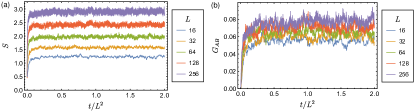
Figure S2: Early-time dependence of (a) half-chain entanglement entropy $S$ and (b) particle-number covariance $G_{AB}$ for the measurement-only model ($\gamma=\infty$) at $\theta=\pi$. The system is initialized at $t=0$ and then evolves due to monitoring.

Example results for the time dependence of the half-chain entropy $S$ and the particle-number covariance $G_{AB}$ are shown in Fig. S2. We can see that numerically, the equilibration period, before the steady state is reached, is roughly $t_{\text{equil}}=L^{2}$. We average the results over the time range between $t_{\text{equil}}$ and $t_{\text{equil}}+200$, and over 1000 random realizations (of the measurement and the initial state) for $L<320$ and 100 realizations for $L=320$. We also find that the time discretization of $dt=0.05$ accurately describes continuous evolution for $\gamma<1$, while we use $dt=0.02$ for $\gamma\geq 1$ and the measurement-only model.

References

- Li et al. [2018] Y. Li, X. Chen, and M. P. A. Fisher, Quantum Zeno effect and the many-body entanglement transition, Phys. Rev. B 98, 205136 (2018).
- Skinner et al. [2019] B. Skinner, J. Ruhman, and A. Nahum, Measurement-induced phase transitions in the dynamics of entanglement, Phys. Rev. X 9, 031009 (2019).
- Chan et al. [2019] A. Chan, R. M. Nandkishore, M. Pretko, and G. Smith, Unitary-projective entanglement dynamics, Phys. Rev. B 99, 224307 (2019).
- Cao et al. [2019] X. Cao, A. Tilloy, and A. De Luca, Entanglement in a fermion chain under continuous monitoring, SciPost Phys. 7, 024 (2019).
- Szyniszewski et al. [2019] M. Szyniszewski, A. Romito, and H. Schomerus, Entanglement transition from variable-strength weak measurements, Phys. Rev. B 100, 064204 (2019).
- Li et al. [2019] Y. Li, X. Chen, and M. P. A. Fisher, Measurement-driven entanglement transition in hybrid quantum circuits, Phys. Rev. B 100, 134306 (2019).
- Bao et al. [2020] Y. Bao, S. Choi, and E. Altman, Theory of the phase transition in random unitary circuits with measurements, Phys. Rev. B 101, 104301 (2020).
- Potter and Vasseur [2022] A. C. Potter and R. Vasseur, Entanglement dynamics in hybrid quantum circuits, in Entanglement in Spin Chains: From Theory to Quantum Technology Applications, edited by A. Bayat, S. Bose, and H. Johannesson (Springer International Publishing, Cham, 2022) pp. 211–249.
- Fisher et al. [2023] M. P. Fisher, V. Khemani, A. Nahum, and S. Vijay, Random quantum circuits, Annu. Rev. Condens. Matter Phys. 14, 335 (2023).
- Alberton et al. [2021] O. Alberton, M. Buchhold, and S. Diehl, Entanglement transition in a monitored free-fermion chain: From extended criticality to area law, Phys. Rev. Lett. 126, 170602 (2021).
- Buchhold et al. [2021] M. Buchhold, Y. Minoguchi, A. Altland, and S. Diehl, Effective theory for the measurement-induced phase transition of Dirac fermions, Phys. Rev. X 11, 041004 (2021).
- Coppola et al. [2022] M. Coppola, E. Tirrito, D. Karevski, and M. Collura, Growth of entanglement entropy under local projective measurements, Phys. Rev. B 105, 094303 (2022).
- Carollo and Alba [2022] F. Carollo and V. Alba, Entangled multiplets and spreading of quantum correlations in a continuously monitored tight-binding chain, Phys. Rev. B 106, L220304 (2022).
- Szyniszewski et al. [2023] M. Szyniszewski, O. Lunt, and A. Pal, Disordered monitored free fermions, Phys. Rev. B 108, 165126 (2023).
- Poboiko et al. [2023] I. Poboiko, P. Pöpperl, I. V. Gornyi, and A. D. Mirlin, Theory of free fermions under random projective measurements, Phys. Rev. X 13, 041046 (2023).
- Poboiko et al. [2024] I. Poboiko, I. V. Gornyi, and A. D. Mirlin, Measurement-induced phase transition for free fermions above one dimension, Phys. Rev. Lett. 132, 110403 (2024).
- Chahine and Buchhold [2024] K. Chahine and M. Buchhold, Entanglement phases, localization, and multifractality of monitored free fermions in two dimensions, Phys. Rev. B 110, 054313 (2024).
- Lumia et al. [2024] L. Lumia, E. Tirrito, R. Fazio, and M. Collura, Measurement-induced transitions beyond Gaussianity: A single particle description, Phys. Rev. Res. 6, 023176 (2024).
- Starchl et al. [2024] E. Starchl, M. H. Fischer, and L. M. Sieberer, Generalized Zeno effect and entanglement dynamics induced by fermion counting (2024), arXiv:2406.07673 [quant-ph] .
- Fava et al. [2024] M. Fava, L. Piroli, D. Bernard, and A. Nahum, Monitored fermions with conserved charge, Phys. Rev. Res. 6, 043246 (2024).
- Jian et al. [2023] C.-M. Jian, H. Shapourian, B. Bauer, and A. W. W. Ludwig, Measurement-induced entanglement transitions in quantum circuits of non-interacting fermions: Born-rule versus forced measurements (2023), arXiv:2302.09094 [cond-mat.stat-mech] .
- Fava et al. [2023] M. Fava, L. Piroli, T. Swann, D. Bernard, and A. Nahum, Nonlinear sigma models for monitored dynamics of free fermions, Phys. Rev. X 13, 041045 (2023).
- Guo et al. [2024] H. Guo, M. S. Foster, C.-M. Jian, and A. W. W. Ludwig, Field theory of monitored, interacting fermion dynamics with charge conservation (2024), arXiv:2410.07317 [cond-mat.stat-mech] .
- Poboiko et al. [2025] I. Poboiko, P. Pöpperl, I. V. Gornyi, and A. D. Mirlin, Measurement-induced transitions for interacting fermions, Phys. Rev. B 111, 024204 (2025).
- Tiutiakina et al. [2024] A. Tiutiakina, H. Lóio, G. Giachetti, J. De Nardis, and A. De Luca, Field theory for monitored Brownian SYK clusters (2024), arXiv:2410.08079 [cond-mat.stat-mech] .
- Ippoliti et al. [2022] M. Ippoliti, T. Rakovszky, and V. Khemani, Fractal, logarithmic, and volume-law entangled nonthermal steady states via spacetime duality, Phys. Rev. X 12, 011045 (2022).
- Block et al. [2022] M. Block, Y. Bao, S. Choi, E. Altman, and N. Y. Yao, Measurement-induced transition in long-range interacting quantum circuits, Phys. Rev. Lett. 128, 010604 (2022).
- Sharma et al. [2022] S. Sharma, X. Turkeshi, R. Fazio, and M. Dalmonte, Measurement-induced criticality in extended and long-range unitary circuits, SciPost Phys. Core 5, 023 (2022).
- Richter et al. [2023] J. Richter, O. Lunt, and A. Pal, Transport and entanglement growth in long-range random clifford circuits, Phys. Rev. Res. 5, L012031 (2023).
- de Albornoz et al. [2024] A. C. C. de Albornoz, D. C. Rose, and A. Pal, Entanglement transition and heterogeneity in long-range quadratic Lindbladians, Phys. Rev. B 109, 214204 (2024).
- Russomanno et al. [2023] A. Russomanno, G. Piccitto, and D. Rossini, Entanglement transitions and quantum bifurcations under continuous long-range monitoring, Phys. Rev. B 108, 104313 (2023).
- Lunt and Pal [2020] O. Lunt and A. Pal, Measurement-induced entanglement transitions in many-body localized systems, Phys. Rev. Research 2, 043072 (2020).
- Van Regemortel et al. [2021] M. Van Regemortel, Z.-P. Cian, A. Seif, H. Dehghani, and M. Hafezi, Entanglement entropy scaling transition under competing monitoring protocols, Phys. Rev. Lett. 126, 123604 (2021).
- Ippoliti et al. [2021] M. Ippoliti, M. J. Gullans, S. Gopalakrishnan, D. A. Huse, and V. Khemani, Entanglement phase transitions in measurement-only dynamics, Phys. Rev. X 11, 011030 (2021).
- Klocke and Buchhold [2023] K. Klocke and M. Buchhold, Majorana loop models for measurement-only quantum circuits, Phys. Rev. X 13, 041028 (2023).
- Note [1] A similar measurement operator was employed in a model of monitored Majorana fermions [43, 21, 22, 44], which violates the U(1) symmetry: there, a superposition of Majorana operators at adjacent cites was considered.
- [37] See Supplemental Material, which includes details of the theoretical analysis and computational approach, and which includes Refs. [45].
- Klich and Levitov [2009] I. Klich and L. Levitov, Quantum noise as an entanglement meter, Phys. Rev. Lett. 102, 100502 (2009).
- Gattenlöhner et al. [2016] S. Gattenlöhner, I. V. Gornyi, P. M. Ostrovsky, B. Trauzettel, A. D. Mirlin, and M. Titov, Lévy flights due to anisotropic disorder in graphene, Phys. Rev. Lett. 117, 046603 (2016).
- Wang et al. [2024] Y.-P. Wang, J. Ren, and C. Fang, Superdiffusive transport on lattices with nodal impurities, Phys. Rev. B 110, 144201 (2024).
- Wang et al. [2023] Y.-P. Wang, C. Fang, and J. Ren, Superdiffusive transport in quasi-particle dephasing models (2023), arXiv:2310.03069 [cond-mat.stat-mech] .
- Wang et al. [2025] Y.-P. Wang, J. Ren, S. Gopalakrishnan, and R. Vasseur, Superdiffusive transport in chaotic quantum systems with nodal interactions (2025), arXiv:2501.08381 [cond-mat.stat-mech] .
- Kells et al. [2023] G. Kells, D. Meidan, and A. Romito, Topological transitions in weakly monitored free fermions, SciPost Phys. 14, 031 (2023).
- Merritt and Fidkowski [2023] J. Merritt and L. Fidkowski, Entanglement transitions with free fermions, Phys. Rev. B 107, 064303 (2023).
- Mirlin et al. [1996] A. D. Mirlin, Y. V. Fyodorov, F.-M. Dittes, J. Quezada, and T. H. Seligman, Transition from localized to extended eigenstates in the ensemble of power-law random banded matrices, Phys. Rev. E 54, 3221 (1996).
- Brezin et al. [1976] E. Brezin, J. Zinn-Justin, and J. C. L. Guillou, Critical properties near dimensions for long-range interactions, J. Phys. A: Math. Gen. 9, L119 (1976).
- Kuznetsov [2011] A. Kuznetsov, On extrema of stable processes, Ann. Probab. 39, 1027 (2011).