Statistical Privacy

Abstract

To analyze the privacy guarantee of personal data in a database that is subject to queries it is necessary to model the prior knowledge of a possible attacker. Differential privacy considers a worst-case scenario where he knows almost everything, which in many applications is unrealistic and requires a large utility loss.

This paper considers a situation called statistical privacy where an adversary knows the distribution by which the database is generated, but no exact data of all (or sufficient many) of its entries. We analyze in detail how the entropy of the distribution guarantes privacy for a large class of queries called property queries. Exact formulas are obtained for the privacy parameters. We analyze how they depend on the probability that an entry fulfills the property under investigation. These formulas turn out to be lengthy, but can be used for tight numerical approximations of the privacy parameters. Such estimations are necessary for applying privacy enhancing techniques in practice. For this statistical setting we further investigate the effect of adding noise or applying subsampling and the privacy utility tradeoff. The dependencies on the parameters are illustrated in detail by a series of plots. Finally, these results are compared to the differential privacy model.

1 Introduction

In many fields like medicine or social sciences research is not possible without access to personal data. One solution is to anonymize databases by techniques like microaggregation to achieve $k$-anonymity or variants of it and then make such a modified database publicly available.

Alternatively one could keep the database secret, but allow certain queries about it. Depending on the type of queries and prior knowledge how much information about individual entries can be deduced from the answers?

The extreme case where the adversary knows almost everything about the database is modeled by the differential privacy setting [9, 8]. This is a pessimistic worst case scenario rarely occurring in practice where queries should not be answered precisely because then the adversary could easily determine the properties of the critical entry. Instead one has to distort the answer in some way.

What are suitable techniques for the distortion that on the one hand leave much uncertainty for an adversary and thus keeps the privacy of individuals, but on the other hand still enable researchers to deduce appropriate results – the tradeoff privacy versus utility [12]? If in this scenario good privacy can be guaranteed without significant loss of utility the problem would have been solved. However, in many cases the utility loss seems to be too severe. Hence, more realistic scenarios than this worst case might be better suited to solve the problem in practice [7]. For other subtleties of differential privacy see [13]. Alternatives to this strong privacy notion have been proposed since then. [7] gives a lists of more than 200 such privacy definitions and states their most important properties and relations as far as known.

The goal of this paper is to mathematically analyze a privacy notion that we consider most suitable for many practical applications and compare its privacy parameters with the one of differential privacy. Our alternative privacy setting assumes that an adversary does not know all details about the entries. His prior information (also called background knowledge) is limited and called passive partial knowledge differential privacy in [6]. The adversary knows the distribution by which the database has been generated and possibly some additional information. For a rigorous mathematical analysis we will concentrate on the underlying distribution and do not consider any other unspecified information. In [4] this situation is called noiseless privacy.

But we want to consider the option to increase privacy by adding noise or other techniques and refer to this setting as statistical privacy. It is similar to the notion (inference-based) distributional differential privacy of [3], but instead of a simulator here we compare conditional distributions directly. We refer to this setting as statistical privacy. We consider the case that an adversary knows the distribution of each entry exactly. These distributions can differ.

Some entries may even be fixed by restricting the support of their distribution to a single value. Thus, even background knowledge that fully specifies certain other entries can be handled. Differential privacy is the extreme case that all entries are fixed except the critical one. Then for an adversary there is no uncertainty caused by the entropy of the database distribution.

A suitable setting should be more realistic for many applications. If the entropy of a given distribution is not sufficient for specific privacy requirements one could add a privacy mechanism to get better bounds. Now the hope is that already for distributions with some entropy good privacy properties can be achieved with less distortion by noise or other techniques. The goal of this paper to analyze precisely how much privacy amplification can be achieved and how much utility is lost for this. We consider a generic class of database queries called counting or property queries. The databases may have any number of attributes with arbitrary dependencies among them to characterize its entries. A property query may select arbitrary combinations of attributes and ask for the number (percentage) of entries that fulfill this condition – in the following called positive entries with respect to this query.

One of our main results is a precise characterization of the privacy loss with respect to the probability of positive entries. Thus we can give privacy guarantees, for example, for medical data when researchers want to investigate rare diseases.

How much the addition of noise generated by classical distributions like Laplace or Gaussian can increase the privacy guarantee has been investigated in a series of papers (for example see [8]). Subsampling is another technique that has been considered [2, 10]. This paper investigates these mechanisms in the statistical setting. It turns out that the analysis gets significantly more complicated than in a worst case scenario. We derive mathematical formulas for the privacy parameters. In case that they cannot be given in a simple closed form the results of numerical approximations are presented to compare the different options. Among others it is shown that the additional entropy in the statistical setting significantly improves the privacy. Furthermore, subsampling compares favorably to artificial noise. Such explicit bounds have been missing for most privacy notions, but are essential for application in practice. In addition the utility loss caused by mechanisms has hardly been investigated. We evaluate this tradeoff and compare the privacy enhancement of mechanisms when they generate the same utility loss.

This paper is organized as follows. The next section introduces the formal setup for querying databases. In Section 3 we define privacy notions, in particular introduce the statistical privacy setting. Then mechanism to amplify privacy are analyzed and we try to obtain closed formulas for the corresponding parameters and the utility loss. Since this is not always possible Section 5 and 6 present the results of numerical approximations of these parameters. This way we provide a comparison between differential and statistical privacy and between noise mechanisms and subsampling to better understand the implications in practice. The paper closes with an outlook for further research on these issues.

2 Databases and Queries

The following setting will be used in this paper to model privacy issues with respect to querying databases.

Definition 1 (Databases and Queries)

An entry $I$ of a database is specified by $d$ attributes. Formally, it is a vector of the space $W\mathrel{\ =\ }W^{(1)}\times\ldots\times W^{(d)}$, where $W^{(i)}$ are the possible values of the $i$-th attribute. Then an entry is given by $I=(w_{1},\ldots,w_{d})$ with $w_{i}\in W^{(i)}$. There can be any dependencies among the attributes.

A database $D$ of size $n$ is a sequence of entries $I_{1},\ldots,I_{n}$. There may be some prior information how a specific database looks like given by a distribution, resp. density function $\mu=(\mu_{1},\ldots,\mu_{n})$ on $W^{n}$, where $\mu_{j}$ is the marginal distribution of the $j$-th entry. To reduce notation, in this paper we use the same symbols for a distribution and its density function if it is clear from the context. By $\mu_{j,\alpha}$ we denote the distribution where $\mu_{j}\equiv\alpha$ is fixed to a constant value $\alpha$ of the support of $\mu_{j}$ denoted by $\operatorname{supp}(\mu_{j})$.

Let $\mathcal{F}$ be a set of queries that may be asked for a given database. Formally, this is described by measurable functions $F:\;W^{n}\mapsto A$, where $A$ denotes an appropriate set of possible answers.

A precise analysis of the information gain of an adversary when querying a database looks hopeless if the distribution $\mu$ can be arbitrarily complex. There may be some dependency between entries of a database, for example if it contains twins that share many personal attributes. In many cases it is still realistic to assume that the entries are independent which will be assumed in the following. Attributes, however, may have arbitrary dependencies between each other.

If queries are allowed that are specific to certain entries of a database like “the age of the second entry” or “the number of female entries $I_{j}$ where the position $j$ is divisible by $3$” it is impossible to guarantee individual privacy. Thus, we restrict the adversary to queries $F$ where the order of the entries is irrelevant – that means symmetric functions. In particular, the weight by which an entry influences the result of $F$ is identical for all entries. Otherwise already with simple linear functions like summing up the values of an attribute over all entries, privacy is completely lost. An adversary even not knowing anything about the database may ask two queries, where in the second one the weight of the critical entry is slightly changed, and from this he can determine the value of that attribute exactly. Thus, symmetry is a natural restriction and prevents that precise information about single entries can be obtained by such simple queries.

For symmetric functions the sequence of arguments $I_{j}$ can be replaced by a multiset or alternatively by a histogram for all possible values of $W$. To extract information from a database one can consider specific properties $U$ and ask for the number or percentage of entries that have property $U$ (a counting query). A property $U$ can be any subset of $W$. Define $\mu_{j}(U):=\sum_{w\in U}\mu_{j}(w)$ as the prior probability that the $j$-entry has property $U$. A property is nontrivial if there is a nonempty set of entries such that $\mu_{j}(U)\not=0$ or $1$. In the following we consider only nontrivial property queries. For trivial properties one obviously does not have to query the database.

Definition 2 (Property Query)

A property query $F$ is described by a subset $W_{F}\mathrel{\subseteq}W$. The correct answer for $F$ given a database $D=I_{1},\ldots,I_{n}$ is the value $y_{F}\mathrel{\ =\ }y_{F}(D)\ :=\ |\{j\;|\;I_{j}\in W_{F}\}|/n\ .$

If $D$ is not fixed, but distributed according to a distribution $\mu$ then the correct answer is a random variable $Y_{F}^{\mu}$ with expectation ${\rm E}\left[Y_{F}^{\mu}\right]=\sum_{j}\mu_{j}(W_{F})/n$. In case that all prior probabilities $\mu_{j}(W_{F})$ are identical to some value $\pi$ such a property query $F$ will be denoted by $F^{\pi}$.

To protect entries and their attributes one could distort the correct answer by applying a function $M$ called mechanism to generate a distribution around $y_{F}(D)$. Let $Y_{F,M}^{\mu}$ denote this random variable.

Note that $Y_{F,M}^{\mu}$ has two sources of randomness: the distribution $\mu$ of $D$ and the deviation generated by $M$.

Property queries are a generic type of queries that can simulate almost every sensible exploration of databases by symmetric queries. For example, if one is interested in the average or median value of a certain attribute listed in a database, by a sequence of property queries with thresholds for this attribute (the percentage of entries that have at least a certain value for this attribute) a histogram can be obtained from which the answer to these questions can be approximated arbitrarily. This extends to combinations of attributes, too. With respect to privacy guarantees, properties with very low or high probability – for example being very rich or having a rare disease – could be critical. This dependency will be part of the following analysis.

A single query $F$ might provide only little information about the entries. To get more information a database might be queried several times called composition of queries or interactive protocol [4, 1, 14, 16]. An important question is the rate by which privacy is reduced in this case. This paper is restricted to the case of single queries. Composition in the statistical setting is even more complex to analyze mathematically and will be subject of further research.

3 Privacy

To measure the privacy loss of entries contained in a database $D$ after it has been queried we want to estimate the information an adversary can deduce from the answers. This obviously depends on the levels of prior information of the adversary. He may have no information at all, thus can only choose the queries to be answered by the curator of the database.

If an adversary has some background information and already knows certain entries of $D$ let $D^{n^{\prime}}$be the database consisting of the remaining $n^{\prime}$ unknown entries. For a query $F$ he can consider the restriction of $F$ to $D^{n^{\prime}}$ and then correct the answer according to the values of the known entries. Knowing some entries reduces the uncertainty of the adversary. The privacy analysis can proceed in the same way by taking the marginal distribution of the database conditioned on the knowledge of the adversary. In the simplest case we consider only the entropy of the entries that are completely unknown.

The strongest nontrivial adversary one can think of knows all entries exactly except one $I_{j}$ and tries to deduce as much information about its attributes as possible. An easier task is a decision problem, namely to decide given a fixed vector $\alpha\in W$ whether the critical entry has these properties. In other words, whether a known individual with attributes $\alpha$ is contained in the database. If this is still hard for an adversary the privacy of the critical entry is saved when it equals $\alpha$. This privacy setting been defined as follows.

Definition 3 (Differential Privacy)

A query $F$ together with a mechanism $M$ is called $(\varepsilon,\delta)$-differential private for a set $\mathcal{D}\mathrel{\subseteq}W^{n}$ of possible databases if for all $(I_{1},\ldots,I_{n})$, all $\alpha,\beta\in W$ and $j\in[1\ldots n]$ such that $D=(I_{1},\ldots,I_{j}=\alpha,\ldots,I_{n})$ and $D^{\prime}=(I_{1},\ldots,I_{j}=\beta,\ldots,I_{n})$ belong to $\mathcal{D}$ and all $S\mathrel{\subseteq}A$, holds

$${\rm Pr}\left[Y_{F,M}\in S\mid D\right]\mathrel{\ \leq\ }e^{\varepsilon}\ {\rm Pr}\left[Y_{F,M}\in S\mid D^{\prime}\right]+\delta\ ,$$

in other words the distribution for $D$ and $D^{\prime}$ are $(\varepsilon,\delta)$-indistinguishable.

If one can guarantee differential privacy with small parameters $\varepsilon,\delta$ against such a strong adversary the entries are protected in an optimal way. However, in general this requires a large distortion by the mechanism $M$ which decreases the utility of the answer significantly. In reality, an adversary in most cases has less prior information about the database.

Definition 4 (Statistical Privacy)

A query $F$ together with a mechanism $M$ is called $(\varepsilon,\delta)$-statistical private for a distribution $\mu$ (or a set of distributions $\mu$) if for all $j\in[1\ldots n]$, $S\mathrel{\subseteq}A$, $\alpha,\beta\in\operatorname{supp}(\mu_{j})$ holds

$${\rm Pr}_{\mu_{j,\alpha}}\left[Y_{F,M}\in S\right]\mathrel{\ \leq\ }e^{\varepsilon}\ {\rm Pr}_{\mu_{j,\beta}}\left[Y_{F,M}\in S\right]+\delta\ ,$$

this means the conditional distributions by fixing the $j$-entry to $\alpha$, resp. $\beta$ are $(\varepsilon,\delta)$-indistinguishable. If there is no mechanism involved, that is we consider $Y_{F}$ distributed according to $\mu$, the query $F$ is called $(\varepsilon,\delta)$-pure statistical private.

Note that our definition of pure statistical privacy is different from noiseless privacy given in [4] to avoid problems with post-processing as discussed in [13]. This issue has already been observed in [3] and fixed. Let us restate two fundamental properties of this privacy notion called privacy axioms in [12]. Using techniques of [6] it can easily been shown.

Lemma 1

For every distribution $\mu$ holds:

• Post-processing: If a query $F$ and a mechanism $M$ are $(\varepsilon,\delta)$-statistical private and $g$ is a random function from the output space $Z$ of queries to a set $Z^{\prime}$ then $g\circ(F,M)$ is $(\varepsilon,\delta)$-statistical private, too.

• Convexity: For any two queries $F_{1}$ and $F_{2}$ with mechanisms $M_{1}$ and $M_{2}$ that are $(\varepsilon,\delta)$-statistical private the query mechanism $(F,M)$ defined by $(F,M)=(F_{1},M_{1})$ with probability $p$ and $(F,M)=(F_{2},M_{2})$ with probability $1-p$ is $(\varepsilon,\delta)$-statistical private.

For property queries the privacy notion can be simplified. For a query $F$ let $\mu_{j}^{{+}}$ (resp. $\mu_{j}^{-}$) be the conditional distribution of $\mu$, where $I_{j}$ is an entry that belongs (resp. does not) to $W_{F}$. Now we measure the information gain obtained by the adversary, the privacy loss, by the difference of $y_{F,M}$ for $\mu_{j,+}$ and $\mu_{j,-}$, and require

$${\rm Pr}_{\mu_{j,+}}\left[Y_{F,M}\in S\right]\leq e^{\varepsilon}\ {\rm Pr}_{\mu_{j,-}}\left[Y_{F,M}\in S\right]+\delta\hbox{ \ and}$$ (1)

$${\rm Pr}_{\mu_{j,-}}\left[Y_{F,M}\in S\right]\leq e^{\varepsilon}\ {\rm Pr}_{\mu_{j,+}}\left[Y_{F,M}\in S\right]+\delta\ .$$ (2)

Definition 5

Let $Y_{F,M}:\;\Omega\mathrel{\rightarrow}Z$ be a random variable for a property query $F$ and mechanism $M$. $\nu_{1},\nu_{2}$ are distributions on $\Omega$ and ${\nu_{i}}^{{F,M}}$ the distributions, resp. density functions of $Y_{F,M}$ with respect to $\nu_{i}$. Then for $z\in Z$ the privacy loss random variable (PLRV) [15] of $F$ and $M$ with resp. to $\nu_{1},\nu_{2}$ is defined as

$$\mathcal{L}^{F,M}_{\nu_{1},\nu_{2}}(z)\ :=\ \ln\ \frac{\nu_{1}^{{F,M}}(z)}{\nu_{2}^{{F,M}}(z)}\ ,$$

where $\ln\frac{0}{0}:=0$ and $\ln\frac{>0}{0}:=\infty$. Given $F,M,\nu_{1},\nu_{2}$ we define the privacy curve by the following function for $\varepsilon\geq 0$

$$\delta_{F,M,\nu_{1},\nu_{2}}(\varepsilon)\ :=\ \int_{Z}\mu^{F,M}_{\nu_{1}}(z)\cdot\max(\;0,\;1-\;{\mathop{\rm exp}\nolimits}\,(\varepsilon-\mathcal{L}^{F,M}_{\nu_{1},\nu_{2}}(z)))\mathbf{d}z\ .$$ (3)

If $\delta\geq\underset{j}{\max}\underset{\alpha,\beta\;\in\;\operatorname{supp}(\mu_{j})}{\sup}\delta_{F,M,\mu_{j,\alpha},\mu_{j,\beta}}(\varepsilon)$ we call $(\varepsilon,\delta)$ an achievable privacy pair for $(F,M)$ and $\mu$.

In [2] the privacy curve is called privacy profile. For property queries the condition on $\delta$ can be simplified to

$$\delta\geq\max\{\delta_{F,M,\mu_{+},\mu_{-}}(\varepsilon),\;\delta_{F,M,\mu_{-},\mu_{+}}(\varepsilon)\}\ .$$ (4)

Lemma 2

For every distribution $\mu$ holds: If $(\varepsilon,\delta)$ is an achievable pair for $(F,M)$ then $(F,M)$ is $(\varepsilon,\delta)$ statistical private.

Proof

The inequality in (1) can be rewritten as

$$\delta \geq\max_{S}\left\{{\rm Pr}_{\mu_{j,\alpha}}\left[Y_{F,M}\in S\right]-e^{\varepsilon}{\rm Pr}_{\mu_{j,\beta}}\left[Y_{F,M}\in S\right]\right\}$$

$$=\max_{S}\left\{\int_{S}\mu_{j,\alpha}(z)-e^{\varepsilon}\ \mu_{j,\beta}(z)\ \mathbf{d}z\right\}=\max_{S}\left\{\int_{S}\mu_{j,\alpha}(z)\ \left(1-e^{\varepsilon}\nobreakspace\ \frac{\mu_{j,\beta}(z)}{\mu_{j,\alpha}(z)}\right)\ \mathbf{d}z\right\}\ .$$

The maximizing set $S\mathrel{\subseteq}Z$ it given by $\displaystyle S_{max}:=\left\{z\mid e^{\varepsilon}\mathrel{\ \leq\ }\frac{\mu_{j,\alpha}(z)}{\mu_{j,\beta}(z)}\right\}\ .$ Therefore the condition is equivalent to

$$\delta\geq\int_{Z}\max\left(0,\ \mu_{j,\alpha}(z)\ \left(1-e^{\varepsilon}\nobreakspace\ \frac{\mu_{j,\beta}(z)}{\mu_{j,\alpha}(z)}\right)\right)\ \mathbf{d}z=\int_{Z}\max\left(0,\ \mu_{j,\alpha}(z)\ \left(1-\frac{e^{\varepsilon}}{\nobreakspace e^{\ln\frac{\mu_{j,\alpha}(z)}{\mu_{j,\beta}(z)}}}\right)\right)\ \mathbf{d}z\ .$$

Combining Definition 4 and Lemma 2 we get

Lemma 3

Given $\mu$, a property query $F$ and a mechanism $M$ are $(\varepsilon,\delta)$-statistical private iff for all $j\in[1\ldots n]$ and all $\alpha,\beta\in\operatorname{supp}(\mu_{j})$ holds $\delta\mathrel{\ \geq\ }\delta_{F,M,\mu_{j,\alpha},\mu_{j,\beta}}(\varepsilon)\ .$

The next section derives explicit formulas for $\delta_{F,M,\mu_{j,\alpha},\mu_{j,\beta}}(\varepsilon)$ for property queries $F$ and the mechanisms that have mainly been considered so far. The pure case without any mechanism can technically be interpreted as a special case of subsampling. Thus, we start with subsampling and afterwards consider pure statistical privacy.

4 Mechanisms

Several mechanisms to guarantee privacy have been analyzed. One technique is adding external noise to the correct answer of a query. The amount of noise depends on the diversity of the entries in the database. If this is large, to achieve differential privacy the distortion of the answers has to be quite large, too. On the contrary, in the noiseless privacy setting exact results are returned – the entropy of the database distribution is used to confuse an adversary.

This section considers property queries and estimates precisely how much the entropy generated by the distribution guarantees statistical privacy and how much this can be enlarged by mechanisms based on noise and subsampling. To keep the mathematical formulas manageable we restrict the analysis to the case that the probability $\pi$ for fulfilling the property is identical for all entries.

4.1 Subsampling

Subsampling means that the answer to a query is derived from a random sample of size $m<<n$ of the entries. The curator does not compute the exact answer to a query, instead applies a corresponding function to the subsample drawn. Let us denote this privacy mechanism by SAMP – among others it has been considered in [17, 10]. Some adjustment might be necessary, for example for counting queries returning the total number since a set of smaller size is considered. For property queries this is not necessary since the ratio is computed. From an exact answer, however, the size of the subsample might be deduced since this is a multiple of $1/m$. If no additional noise is added this can be prevented if $m$ is chosen as a divisor of $n$. Our analysis below does not require that $m$ is unknown to an adversary. Here we consider only sampling without replacement. Similar results hold with replacement if $m$ is significantly smaller than $n$ ($<\sqrt{n}$).

Given a database $D$ of size $n$ and a property query $F$ we have defined $y_{F}=y_{F}(D)$, resp. $\pi_{F}$ as the portion of positive elements in $D$. Let us define  $\xi:=\pi_{F}/(1-\pi_{F})$ as the relation between positive and negative elements for a given database $D$. Furthermore, let $a_{F,m}$ denote the random variable that gives the portion of positive elements in a random sample $D^{m}$, which can take values $j/m$ with $j\in[0\ldots m]$ and is hypergeometric distributed. This means

$${\rm Pr}\left[a_{F,m}=j/m\right]\mathrel{\ =\ }\frac{\binom{y_{F}\;n}{j}\ \binom{(1-y_{F})\;n}{m-j}}{\binom{n}{m}}$$

with expectation $y_{F}$ and variance $m^{-1}\;y_{F}\;(1-y_{F})\;\frac{n-m}{n-1}\mathrel{\ \leq\ }1/4m$. For $m\leq 0.05\;n$ the distribution of $a_{F,m}$ is well approximated by the binomial distribution for $m$ independent draws and success probability $y_{F}$. Thus, ${\rm Pr}\left[a_{F,m}=j/m\right]\mathrel{\ \approx\ }\binom{m}{j}\ y_{F}^{\ j}\ (1-y_{F})^{m-j}\ .$ The expectation of this binomial distribution is given by $y_{F}$ and its variance by $m^{-1}\;y_{F}\;(1-y_{F})$. To simplify the calculation one can use this approximation for a fixed database.

Now consider subsampling for a database $D$ when it is known that the critical element is positive (resp. negative). Due to symmetry one can restrict the analysis to the case that the first element is the critical one. Let $y_{F}$ be the ratio of positive elements in the remaining $n-1$ ones. Then we distinguish whether the first element is drawn or not – the first case happening with probability $\lambda=m/n$. This gives

$${\rm Pr}\left[a_{F,m}=\frac{j}{m}\;|\;D_{1}\in W^{F}\right] \approx\lambda\;\binom{m-1}{j-1}\ y_{F}^{\ j-1}\;(1-y_{F})^{m-j}+(1-\lambda)\;\binom{m}{j}\ y_{F}^{\ j}\;(1-y_{F})^{m-j}$$

$${\rm Pr}\left[a_{F,m}=\frac{j}{m}\;|\;D_{1}\notin W^{F}\right] \approx\lambda\;\binom{m-1}{j}\ y_{F}^{\ j}\ (1-y_{F})^{m-j-1}+(1-\lambda)\;\binom{m}{j}\ y_{F}^{\ j}\;(1-y_{F})^{m-j}$$

The quotient of the right sides can be simplified to

$$\frac{{\rm Pr}\left[a_{F,m}=j/m\;|\;D_{1}\in W^{F}\right]}{{\rm Pr}\left[a_{F,m}=j/m\;|\;D_{1}\notin W^{F}\right]}$$

$$\approx\ \frac{\lambda\ \binom{m-1}{j-1}\ y_{F}^{\ j-1}\;(1-y_{F})^{m-j}+(1-\lambda)\;\binom{m}{j}\ y_{F}^{\ j}\;(1-y_{F})^{m-j}}{\lambda\ \binom{m-1}{j}\ y_{F}^{\ j}\ (1-y_{F})^{m-j-1}+(1-\lambda)\;\binom{m}{j}\ y_{F}^{\ j}\;(1-y_{F})^{m-j}}$$

$$\mathrel{\ =\ }\frac{\lambda\;j\ \;(1-y_{F})+(1-\lambda)\;m\;y_{F}\;(1-y_{F})}{\lambda\;(m-j)\;\xi\;(1-y_{F})+(1-\lambda)\;m\;y_{F}\;(1-y_{F})}=\frac{\lambda\;j+(1-\lambda)\;m\;y_{F}}{\lambda\;(m-j)\;\xi+(1-\lambda)\;m\;y_{F}}\ ,$$

which is monoton increasing in $j$.

Now assume that subsampling is performed for a property query $F$ with a random database $D$ drawn from a distribution $\mu$ where each entry is positive with probability $\pi_{F}$. Let $\xi=\pi_{F}/(1-\pi_{F})$ and $\mu_{+}$ and $\mu_{-}$ be the marginal distribution of $\mu$ when the critical element is positive, resp. negative. For these densities we get the same expression as above:

$${\rm Pr}_{\mu_{+}}\left[a_{F,m}=j/m\right] \mathrel{\ =\ }\lambda\ \binom{m-1}{j-1}\ \pi_{F}^{\ j-1}\;(1-\pi_{F})^{m-j}+(1-\lambda)\;\binom{m}{j}\ \pi_{F}^{\ j}\;(1-\pi_{F})^{m-j}$$

$${\rm Pr}_{\mu_{-}}\left[a_{F,m}=j/m\right] \mathrel{\ =\ }\lambda\ \binom{m-1}{j}\ \pi_{F}^{\ j}\ (1-\pi_{F})^{m-j-1}+(1-\lambda)\;\binom{m}{j}\ \pi_{F}^{\ j}\;(1-\pi_{F})^{m-j}$$

Define $\displaystyle Q_{+}(j)\ :=\ \frac{{\rm Pr}_{\mu_{+}}\left[a_{F,m}=j/m\right]}{{\rm Pr}_{\mu_{-}}\left[a_{F,m}=j/m\right]}\ .$

Lemma 4

When taking a subsample of size $m$ (without replacement) from a database distribution $\mu$, where each entry independently is positive with probability $\pi_{F}$, then the number of positive elements is binomially distributed with parameters $m$ and $\pi_{F}$. Therefore, the expectation of $Y_{F,{\tt SAMP}}$ is $\pi_{F}$ and its variance $\pi_{F}\;(1-\pi_{F})/m$ .
Furthermore, for the ratio of the marginal distribution holds

$$Q_{+}(j)\mathrel{\ =\ }\frac{\lambda\;j+(1-\lambda)\;m\;\pi_{F}}{\lambda\;(m-j)\;\xi+(1-\lambda)\;m\;\pi_{F}}\ .\\$$

Since we also have to bound the reciprocal fraction let us define $Q_{-}(j)\ :=\ Q(j)^{-1}$. Interpolating $Q_{+}(j)$ to arbitrary rational values $j$ this function takes value $1$ for $j=\pi_{F}\;m$ , which is the expectation of $m\;a_{F,m}$. To determine the privacy curve one has to estimate when the quotients $Q_{+}(j)$ and $Q_{-}(j)$ exceed $e^{\varepsilon}$. For $Q_{+}(j)$ consider a fraction $j=(1+\gamma)\;\pi_{F}m.$ above the expectation where $0\leq\gamma\leq 1/\pi_{F}-1$:

$$Q_{+}((1+\gamma)\;\pi_{F}\;m)\mathrel{\ =\ }\frac{\lambda\;j+(1-\lambda)\;m\;\pi_{F}}{\lambda\;(m-j)\;\xi+(1-\lambda)\;m\;\pi_{F}}$$

$$\mathrel{\ =\ }\frac{\lambda\;(1+\gamma)\;\pi_{F}\;m+(1-\lambda)\;m\;\pi_{F}}{\lambda\;(m-(1+\gamma)\;\pi_{F}\;m)\;\xi+(1-\lambda)\;m\;\pi_{F}}\mathrel{\ =\ }\frac{\lambda\;(1+\gamma)\;\pi_{F}\;m+(1-\lambda)\;m\;\pi_{F}}{\lambda\;(1-(1+\gamma)\;\pi_{F})\;m\;\frac{\pi_{F}}{1-\pi_{F}}+(1-\lambda)\;m\;\pi_{F}}$$

$$\mathrel{\ =\ }\frac{\lambda\;(1+\gamma)+(1-\lambda)}{\lambda\;\frac{1-\pi_{F}-\gamma\;\pi_{F}}{1-\pi_{F}}+(1-\lambda)}\mathrel{\ =\ }\mathrel{\ =\ }\frac{\lambda\;(1+\gamma)+(1-\lambda)}{\lambda\;(1-\frac{\gamma\;\pi_{F}}{1-\pi_{F}})+(1-\lambda)}\mathrel{\ =\ }\frac{1+\lambda\;\gamma}{1-\lambda\;\frac{\gamma\;\pi_{F}}{1-\pi_{F}}}\ .$$

This gives the equation $e^{\varepsilon}\mathrel{\ =\ }Q_{+}((1+\gamma)\;\pi_{F}\;m)\mathrel{\ =\ }\frac{1+\lambda\;\gamma}{1-\lambda\;\frac{\gamma\;\pi_{F}}{1-\pi_{F}}}$ that with respect to $\gamma$ has the solution $\gamma_{+}^{\star}\mathrel{\ =\ }\lambda^{-1}\;\frac{e^{\varepsilon}-1}{1+\;e^{\varepsilon}\;\frac{\pi_{F}}{1-\pi_{F}}}\ .$ Let $\gamma_{+}^{\star\star}:=\min\{\gamma_{+}^{\star},\;1/\pi_{F}-1\}$ and $j_{+}^{\star}\ :=\ (1+\gamma_{+}^{\star\star})\;\pi_{F}\;m$. Then for all $j\leq j_{+}^{\star}$ holds: $Q_{+}(j)\leq e^{\varepsilon}$. Now the privacy curve $\delta_{+}(\varepsilon)=\delta_{F,M_{{\tt SAMP}},\mu_{+},\mu_{-}}(\varepsilon)$ as defined in (3) and (4) simplifies to

$$\delta_{+}(\varepsilon) =\sum_{j=\left\lceil j_{+}^{\star}\right\rceil}^{m}{\rm Pr}_{\mu_{+}}\left[Y_{F,{\tt SAMP}}=j/m\right]\ \left(1-\frac{e^{\varepsilon}}{Q_{+}(j)}\right)=\sum_{j=\left\lceil j_{+}^{\star}\right\rceil}^{m}\left({\rm Pr}_{\mu_{+}}\left[Y_{F,{\tt SAMP}}=j/m\right]-e^{\varepsilon}\;{\rm Pr}_{\mu_{-}}\left[Y_{F,{\tt SAMP}}=j/m\right]\right)$$

$$=\sum_{j=\left\lceil j_{+}^{\star}\right\rceil}^{m}\pi_{F}^{j-1}(1-\pi_{F})^{m-j-1}\binom{m-1}{j}\left(\lambda\left(\frac{j(1-\pi_{F})}{m-j}-e^{\varepsilon}\;\pi_{F}\right)+(1-\lambda)(1-e^{\varepsilon})\;\frac{m\;\pi_{F}(1-\pi_{F})}{m-j}\right)$$

Similar calculations hold for the negative case $\delta_{-}(\varepsilon)\mathrel{\ =\ }\delta_{F,M_{{\tt SAMP}},\mu_{-},\mu_{+}}(\varepsilon)$ with the monoton decreasing function $Q_{-}(j)$. Now, for $\gamma\leq 1$ one has to solve

$$Q_{-}((1-\gamma)\;\pi_{F}\;m) =\frac{\lambda\;(m-j)\;\xi+(1-\lambda)\;m\;\pi_{F}}{\lambda\;j+(1-\lambda)\;m\;\pi_{F}}$$

$$=\frac{\lambda\;(m-(1-\gamma)\;\pi_{F}\;m)\;\xi+(1-\lambda)\;m\;\pi_{F}}{\lambda\;(1-\gamma)\;\pi_{F}\;m+(1-\lambda)\;m\;\pi_{F}}=\frac{1+\lambda\;\frac{\gamma\;\pi_{F}}{1-\pi_{F}}}{1-\lambda\;\gamma}\ .$$

The solution is $\displaystyle\gamma_{-}^{\star}\mathrel{\ =\ }\lambda^{-1}\;\frac{1-e^{-\varepsilon}}{1+\;e^{-\varepsilon}\;\frac{\pi_{F}}{1-\pi_{F}}}\ .$ For $\gamma_{-}^{\star\star}:=\min\{\gamma_{-}^{\star},\;1\}$ and $j_{-}^{\star}\ :=\ (1-\gamma_{-}^{\star\star})\;\pi_{F}\;m$ and all $j\geq j_{-}^{\star}$ holds: $Q_{-}(j)\leq e^{\varepsilon}$ . This gives

$$\delta_{-}(\varepsilon)\mathrel{\ =\ }\sum_{j=0}^{\,\left\lfloor j_{-}^{\star}\right\rfloor\,}{\rm Pr}_{\mu_{-}}\left[Y_{F,{\tt SAMP}}=j/m\right]\ \left(1-\frac{e^{\varepsilon}}{Q_{-}(j)}\right)\ .$$

Summarizing we have shown

Theorem 4.1

For databases of size $n$ and property queries $F$ with probability $\pi_{F}$ for an entry being positive, subsampling with rate $\lambda$ gives the privacy curve $\delta(\varepsilon)=\max\{\delta_{+}(\varepsilon),\;\delta_{-}(\varepsilon)\}$ where

$$\delta_{+}(\varepsilon) \mathrel{\ =\ } \sum_{j=\left\lceil j_{+}^{\star}\right\rceil}^{n\;\lambda}\pi_{F}^{j-1}(1-\pi_{F})^{n\;\lambda-j-1}\binom{n\;\lambda-1}{j}$$

$$\qquad\left(\lambda\left(\frac{j(1-\pi_{F})}{n\;\lambda-j}-e^{\varepsilon}\pi_{F}\right)+(1-\lambda)(1-e^{\varepsilon})\frac{n\;\lambda\;\pi_{F}(1-\pi_{F})}{n\;\lambda-j}\right)\ ,$$

$$\delta_{-}(\varepsilon) \mathrel{\ =\ } \sum_{j=0}^{\left\lceil j_{-}^{\star}\right\rceil}\pi_{F}^{j-1}(1-\pi_{F})^{n\;\lambda-j-1}\binom{n\;\lambda-1}{j}$$

$$\qquad\left(\lambda\left(\pi_{F}-e^{\varepsilon}\frac{j(1-\pi_{F})}{n\;\lambda-j}\right)+(1-\lambda)(1-e^{\varepsilon})\frac{n\;\lambda\;\pi_{F}(1-\pi_{F})}{n\;\lambda-j}\right)\ ,$$

$$j_{+}^{\star} \mathrel{\ =\ } \min\{\lambda,\;\lambda+\frac{e^{\varepsilon}-1}{1+\;e^{\varepsilon}\;\frac{\pi_{F}}{1-\pi_{F}}}\}\;n\;\pi_{F},\ j_{-}^{\star}\mathrel{\ =\ }\max\{0,\;\lambda+\frac{e^{-\varepsilon}-1}{1+\;e^{-\varepsilon}\;\frac{\pi_{F}}{1-\pi_{F}}}\}\;n\;\pi_{F}\ .$$

4.2 Pure Statistical Privacy

In the pure statistical privacy setting there is no mechanism applied to confuse an adversary. The entropy generated by the distribution of databases of size $n$ and property probability $\pi_{F}$ is $H(\pi_{F})\;n$, resp. $H(\pi_{F})\;(n-1)$ if the critical entry is fixed where $H$ denotes the Shannon entropy function. The distribution of the number of positive entries among the remaining $n-1$ entries has variance $\pi_{F}\;(1-\pi_{F})\;n$.

To derive the $(\varepsilon,\delta)$-curve in this case, for the quotient of the two conditional distributions $\mu_{+}$ and $\mu_{-}$ one can use the same formulas as for subsampling by setting $\lambda=1$. This gives (assuming $\varepsilon\leq\ln 2$)

Theorem 4.2

For databases of size $n$ and property queries $F$ with probability $\pi_{F}$ for an entry being positive, pure statistical privacy is guaranteed with $\delta(\varepsilon)=\max\{\delta_{+}(\varepsilon),\;\delta_{-}(\varepsilon)\}$ where

$$\delta_{+}(\varepsilon) \mathrel{\ =\ } \sum_{j=\left\lceil j_{+}^{\star}\right\rceil}^{n}\pi_{F}^{j-1}(1-\pi_{F})^{n-j-1}\binom{n-1}{j}\left(\frac{j(1-\pi_{F})}{n-j}-e^{\varepsilon}\pi_{F}\right)\ ,$$

$$\delta_{-}(\varepsilon) \mathrel{\ =\ } \sum_{j=0}^{\left\lceil j_{-}^{\star}\right\rceil}\pi_{F}^{j-1}(1-\pi_{F})^{n-j-1}\binom{n-1}{j}\left(\pi_{F}-e^{\varepsilon}\frac{j(1-\pi_{F})}{n-j}\right)$$

$$j_{+}^{\star} \mathrel{\ =\ } 1+\frac{e^{\varepsilon}-1}{1+\;e^{\varepsilon}\;\frac{\pi_{F}}{1-\pi_{F}}}\ n\;\pi_{F},\quad j_{-}^{\star}\mathrel{\ =\ }1+\frac{e^{-\varepsilon}-1}{1+\;e^{-\varepsilon}\;\frac{\pi_{F}}{1-\pi_{F}}}\ n\;\pi_{F}\ .$$

Note that the thresholds $j_{+}^{\star}$ and $j_{-}^{\star}$ are a constant fraction away from the expectation of the binomial distribution. Thus, by Chernoff’s bound $\delta(\varepsilon)$ decreases exponentially with respect to $n$.

4.3 Noise

Adding noise to the result of a query is the standard mechanism to enhance privacy. It has been shown that Laplace noise can achieve pure differential privacy(that means $\delta=0$) [8].

Definition 6 (Additive Noise Mechanism)

Let $F$ be a property query and ADN a noise function defined by a a random variable $\mathcal{N}$ with mean $0$ that is independent of the database distribution $\mu$. Then $Y_{F,{\tt ADN}}\ :=\ Y_{F}+\mathcal{N}$ is an additive noise mechanism for $F$. If $\mathcal{N}=Lap(\psi)$ is Laplace distributed with scaling factor $\psi$ and variance $2\psi^{2}$ this mechanism will be denoted by ${\tt LAP}_{\psi}$ and if $\mathcal{N}=N(0,\psi^{2})$ is normal distributed with standard deviation $\psi$ by ${\tt GAU}_{\psi}$.

The strength of the noise only depends on the sensitivity $s$ of the query, the maximal difference between the results of two databases that differ in exactly one entry. For property queries it holds $s=1/n$ for databases of size $n$. In general, $\varepsilon$-differential privacy can be achieved by Laplace noise ${\tt LAP}_{\psi}$ with $\psi=s/\varepsilon$, that means we need noise of scale $1/\varepsilon\;n$ for property queries.

As shown the entropy of the database distribution already guarantees a certain privacy level. How can statistical privacy be improved by adding noise? This section establishes bounds similar to the distributional privacy setting. They are independent of the probability $\pi$ of a property – thus noise may be helpful for very small $\pi$ where not enough entropy is given.

Lemma 5

Let $F$ be a property query for a distribution on databases of size $n$, where each entry is positive independently with some fixed probability $0<\pi<1$. Then for $\psi>0$, $(F,{\tt LAP}_{\psi})$ is $(1/\psi n,0)$–statistical private.

Proof

For every (measurable) set $S$ holds

$${\rm Pr}_{\mu_{+}}\left[Y_{F,{\tt LAP}_{\psi}}\in S\right] =\sum_{j=0}^{n}{\rm Pr}_{\mu_{+}}\left[Y_{F,{\tt LAP}_{\psi}}\in S\;|\;Y_{F}=\frac{j}{n}\right]\quad{\rm Pr}_{\mu_{+}}\left[Y_{F}=\frac{j}{n}\right]$$

$$=\sum_{j=1}^{n}\frac{1}{2\psi}\ \int_{S}e^{-\frac{\left|x-(j/n)\right|}{\psi}}\mathbf{d}x\quad\binom{n-1}{j-1}\ \pi_{F}^{j-1}(1-\pi_{F})^{n-j}$$

$$=\frac{1}{2\psi}\ \int_{S}\ \sum_{j=0}^{n-1}e^{-\frac{\left|x-((j+1)/n)\right|}{\psi}}\binom{n-1}{j}\ \pi_{F}^{j}(1-\pi_{F})^{n-j-1}\mathbf{d}x$$

$${\rm Pr}_{\mu_{-}}\left[Y_{F,{\tt LAP}_{\psi}}\in S\right] =\sum_{j=0}^{n}{\rm Pr}_{\mu_{-}}\left[Y_{F,{\tt LAP}_{\psi}}\in S\;|\;Y_{F}=\frac{j}{n}\right]\quad{\rm Pr}_{\mu_{-}}\left[Y_{F}=\frac{j}{n}\right]$$

$$=\frac{1}{2\psi}\ \int_{S}\ \sum_{j=0}^{n-1}e^{-\frac{\left|x-j/n\right|}{\psi}}\binom{n-1}{j}\ \pi_{F}^{j}(1-\pi_{F})^{n-j-1}\mathbf{d}x\ .$$

Notice that the corresponding summands only differ in the exponential function which can be rewritten as

$$e^{-\frac{\left|x-((j+1)/n)\right|}{\psi}}\mathrel{\ =\ }e^{-\frac{\left|x-(j/n)\right|}{\psi}}\quad e^{\frac{1}{\psi}\underbrace{\left(\left|x-j/n\right|-\left|x-(j+1)/n\right|\right)}_{\zeta(x,j)}}\ ,$$

where the distinguishing function $\zeta(x,j)$ is given

$$\zeta(x,j)=\begin{cases*}-1/n&\text{if $x\leq j/n$},\\ +1/n&\text{if $x\geq(j+1)/n$},\\ 2\;(x-\frac{j+1/2}{n})&\text{else.}\end{cases*}$$

Since $-1/n\leq\zeta(x,j)\leq 1/n$ for all $x$ and $j$ we get

$$e^{-1/\psi n}\ {\rm Pr}_{\mu_{-}}\left[Y_{F,{\tt LAP}_{\psi}}\in S\right]\mathrel{\ \leq\ }{\rm Pr}_{\mu_{+}}\left[Y_{F,{\tt LAP}_{\psi}}\in S\right]\mathrel{\ \leq\ }e^{1/\psi n}\ {\rm Pr}_{\mu_{-}}\left[Y_{F,{\tt LAP}_{\psi}}\in S\right]\ .$$

Note that the bound $e^{1/\psi n}$ is quite tight. If $x\geq 1$ then for all $0\leq j\leq n-1$ holds $x\geq(j+1)/n$ and thus $\zeta(x,j)=1/n$ . Choosing $S=[1,\infty)$ gives

$${\rm Pr}_{\mu_{+}}\left[Y_{F,{\tt LAP}_{\psi}}\in S\right]\mathrel{\ =\ }e^{1/\psi n}\ {\rm Pr}_{\mu_{-}}\left[Y_{F,{\tt LAP}_{\psi}}\in S\right]\ .$$

Thus, statistical privacy requires about the same Laplace noise as differential privacy for $\delta=0$. But what about $(\varepsilon,\delta)$-privacy with $\delta>0$? In the next section we will show that the uncertainty of an adversary based on the database distribution allows significantly smaller $\delta$ for the same $\varepsilon$. Alternatively, one could add Gaussian noise ${\tt GAU}_{\nu s}$ for arbitrary $\nu$. In this case it is not possible to achieve pure differential privacy with $\delta=0$, still the normal distribution has other favorable properties. In the statistical setting we get the following bound on $\delta$ with resp. to $\varepsilon$.

Lemma 6

For databases of size $n$ let $F$ be a property query, where each entry is positive independently with probability $0<\pi<1$. Then the query $(F,{\tt GAU}_{\nu s})$ is $(\varepsilon,\delta)$–statistical private if $\delta\geq\max\{\delta_{F,M,\mu_{+},\mu_{-}}(\varepsilon),\delta_{F,M,\mu_{-},\mu_{+}}(\varepsilon)\}$ where

$$\delta_{F,M,\mu_{+},\mu_{-}}(\varepsilon) \approx {\rm Pr}_{\mu_{+}}\left[Y_{F,M}\geq\pi+n\sigma^{2}\varepsilon+\frac{1/2-\pi}{n}\right]-e^{\varepsilon}\;{\rm Pr}_{\mu_{-}}\left[Y_{F,M}\geq\pi+n\sigma^{2}\varepsilon+\frac{1/2-\pi}{n}\right]$$

$$\delta_{F,M,\mu_{-},\mu_{+}}(\varepsilon) \approx {\rm Pr}_{\mu_{-}}\left[Y_{F,M}\leq\pi-n\sigma^{2}\varepsilon+\frac{1/2-\pi}{n}\right]-e^{\varepsilon}\;{\rm Pr}_{\mu_{+}}\left[Y_{F,M}\leq\pi-n\sigma^{2}\varepsilon+\frac{1/2-\pi}{n}\right]$$

and $\sigma^{2}=(\nu s)^{2}+\pi(1-\pi)(n-1)/n^{2}$.

Proof

For larger $n$ the binomial distribution can be approximated by the Gaussian distribution. Thus, $Y_{F}\approx\mathcal{N}(\pi-\pi/n+1/n,\pi(1-\pi)(n-1)/n^{2})$ with respect to $\mu_{+}$ and $Y_{F}\approx\mathcal{N}(\pi-\pi/n,\pi(1-\pi)(n-1)/n^{2})$ with respect to $\mu_{-}$. Since the convolution of these Gaussians with noise ${\tt GAU}_{\nu s}$ results in a Gaussian with variance $\sigma^{2}=(\nu s)^{2}+\pi(1-\pi)(n-1)/n^{2}$ it holds

$$Y_{F,M}\mid_{\mu_{+}} \approx \mathcal{N}(\pi(1-1/n)+1/n,\sigma^{2})$$

$$Y_{F,M}\mid_{\mu_{-}} \approx \mathcal{N}(\pi(1-1/n),\sigma^{2}).$$

This gives

$$\delta_{F,M,\mu_{+},\mu_{-}}(\varepsilon) \approx\int_{A}\frac{1}{\sqrt{2\pi\sigma^{2}}}\max\left\{0,e^{-\frac{(x-\pi(1-1/n)-1/n)^{2}}{2\sigma^{2}}}-e^{\varepsilon}e^{-\frac{(x-\pi(1-1/n))^{2}}{2\sigma^{2}}}\right\}\mathbf{d}x$$

$$=\int_{A}\frac{e^{-\frac{(x-\pi(1-1/n))^{2}}{2\sigma^{2}}}}{\sqrt{2\pi\sigma^{2}}}\max\left\{0,e^{-\frac{-2xn+2\pi(n-1)+1}{2\sigma^{2}n^{2}}}-e^{\varepsilon}\right\}\mathbf{d}x.$$

The second argument of the $\max$ function is monotone increasing and zero if

$$\varepsilon=-\frac{-2xn+2\pi(n-1)+1}{2\sigma^{2}n^{2}}.$$

This has the solution $x^{\star}=\pi+n\sigma^{2}\varepsilon+(1/2-\pi)/n$ and reduces the integral to

$$\delta_{F,M,\mu_{+},\mu_{-}}(\varepsilon) \approx \int_{x^{\star}}^{\infty}\frac{e^{-\frac{(x-\pi(1-1/n)-1/n)^{2}}{2\sigma^{2}}}}{\sqrt{2\pi\sigma^{2}}}\mathbf{d}x-e^{\varepsilon}\int_{x^{\star}}^{\infty}\frac{e^{-\frac{(x-\pi(1-1/n))^{2}}{2\sigma^{2}}}}{\sqrt{2\pi\sigma^{2}}}\mathbf{d}x$$

$$= {\rm Pr}_{\mu_{+}}\left[Y_{F,M}\geq x^{\star}\right]-e^{\varepsilon}\;{\rm Pr}_{\mu_{-}}\left[Y_{F,M}\geq x^{\star}\right].$$

Using similar calculations we get for $x^{\star\star}=\pi-n\sigma^{2}\varepsilon+(1/2-\pi)/n$

$$\delta_{F,M,\mu_{-},\mu_{+}}(\varepsilon)\approx{\rm Pr}_{\mu_{-}}\left[Y_{F,M}\leq x^{\star\star}\right]-e^{\varepsilon}\;{\rm Pr}_{\mu_{+}}\left[Y_{F,M}\leq x^{\star\star}\right].$$

For a property query $F^{\pi}$ the expectation of $Y_{F,{\tt GAU}_{\psi}}$ is $\pi$. Thus to achieve a small $\delta$, the parameters should be chosen such that ${\rm Pr}_{\mu_{+}}\left[Y_{F,{\tt GAU}_{\psi}}\geq\varepsilon n\psi^{2}+\frac{1}{2n}\right]$ is small, that means the threshold $\varepsilon n\psi^{2}+\frac{1}{2n}$ should be significantly larger than the expectation of $Y_{F,{\tt GAU}_{\psi}}$. This holds if it is larger than $\pi+k\psi$, some multiple $k$ of the standard deviation. Note that the bound for $\delta$ involves the error function for which no simple analytical formula is known.

4.4 Utility Loss

To estimate the tradeoff between privacy amplification and loss of utility for a query $F$ and a database $D$, one measures the deviation to the correct answer $y_{F}(D)$ by the mean squared error (MSE). In the statistical setting we take the expectation over all databases with respect to the distribution $\mu$.

Definition 7 (Utility Loss)

For a query $F$ on databases distributed according to a distribution $\mu$ and a mechanism $M$ the utility loss is given by

$${\rm UL}(F,M)\ :=\ \mathbf{E}_{\mu}\left[\left(Y_{F,M}-Y_{F}\right)^{2}\right].$$

For subsampling this can be estimated as follows.

Lemma 7

For a property query $F^{\pi}$ subsampling with selection probability $\lambda=m/n$ gives  ${\rm UL}(F,{\tt SAMP})\mathrel{\ =\ }\pi(1-\pi)\ (\frac{1}{m}-\frac{1}{n})$.

Proof

The random variables $Y_{F}$ and $Y_{F,M}$ are binomially distributed with expectation $\pi$ and variance $\pi\;(1-\pi)/n$, resp. $\pi\;(1-\pi)/m$ (Lemma 4). To shorten the formulas we drop writing down the distribution $\mu$ when it is clear from the context. Thus,

$$\mathbf{E}_{\mu}\left[\left(Y_{F,{\tt SAMP}}-Y_{F}\right)^{2}\right] =\mathbf{E}\left[\left((Y_{F,{\tt SAMP}}-{\pi})-(Y_{F}-{\pi})\right)^{2}\right]$$

$$=\mathbf{E}\left[\left(Y_{F,{\tt SAMP}}-{\pi}\right)^{2}\right]+\mathbf{E}\left[\left(Y_{F}-{\pi}\right)^{2}\right]-2\;\mathbf{E}\left[(Y_{F,{\tt SAMP}}-{\pi})(Y_{F}-{\pi})\right]$$

$$=\frac{{\pi}(1-{\pi})}{m}+\frac{{\pi}(1-{\pi})}{n}-2\left({\pi}^{2}-{\pi}\;\mathbf{E}\left[Y_{F,{\tt SAMP}}\right]-{\pi}\;\mathbf{E}\left[Y_{F}\right]+\mathbf{E}\left[Y_{F}Y_{F,{\tt SAMP}}\right]\right)$$

$$=\frac{{\pi}(1-{\pi})}{m}+\frac{{\pi}(1-{\pi})}{n}+2{\pi}^{2}-2\;\mathbf{E}\left[Y_{F}\;Y_{F,{\tt SAMP}}\right]\ .$$

The last term can be evaluated by computing the covariance since

$$\mathbf{E}\left[Y_{F}\;Y_{F,{\tt SAMP}}\right]=\mathbf{E}\left[Y_{F}\right]\ \mathbf{E}\left[Y_{F,{\tt SAMP}}\right]+{\rm Cov}\left[Y_{F},\;Y_{F,{\tt SAMP}}\right]$$

Now using the fact that taken random samples $X$ of a set $D$ and evaluating $F$ on $X$ has expectation $y_{F}(D)$ we get

$${\rm Cov}\left[Y_{F},\;Y_{F,{\tt SAMP}}\right]\mathrel{\ =\ }\mathbf{E}\left[(Y_{F}-\mathbf{E}[Y_{F}])\;(Y_{F,{\tt SAMP}}-\mathbf{E}[Y_{F,{\tt SAMP}}])\right]$$

$$=\int_{W^{n}}\left(y_{F}(D)-\mathbf{E}[Y_{F}]\right)\left(\sum_{\mathrlap{x\in{\rm Img}({\tt SAMP}(D))}}\ {\rm Pr}\left[x={\tt SAMP}(D)\right]\;(y_{F}(x)-\mathbf{E}[Y_{F,{\tt SAMP}}])\right)\mathbf{d}\mu(D)$$

$$=\int_{W^{n}}(y_{F}(D)-\pi)\;(y_{F}(D)-\pi)\;\mathbf{d}\mu(D)={\rm Var}[Y_{F}]\mathrel{\ =\ }\frac{{\pi}(1-{\pi})}{n}\ ,\text{\normalsize which gives}$$

$$\mathbf{E}\left[Y_{F}\;Y_{F,{\tt SAMP}}\right]={\pi}^{2}+\frac{{\pi}(1-{\pi})}{n}\phantom{=}\text{and}\phantom{=}\mathbf{E}\left[\left(Y_{F,{\tt SAMP}}-Y_{F}\right)^{2}\right]=\frac{{\pi}(1-{\pi})}{m}-\frac{{\pi}(1-{\pi})}{n}\ .$$

From a statistical point of view evaluating a property $F$ on databases $D$ could be interpreted differently. Namely, we want to estimate the expectation $Y_{F}$ for the given distribution $\mu$. This introduces a certain MSE. Now adding a mechanism $M$ like subsampling increases the MSE. Then the utility loss generated by $M$ should be defined as the increase of the MSE by $M$ compared to the MSE without $M$.

Definition 8 (Statistical Utility Loss)

For a query $F$ on databases distributed according to a distribution $\mu$ and a mechanism $M$ the statistical utility loss is defined as ${\rm UL}_{\tt STAT}(F,M)\ :=\ {\rm MSE}(Y_{F,M})-{\rm MSE}(Y_{F})\ .$

This value can easily be computed.

Lemma 8

Let $F^{\pi}$ be a property query and ${\tt SAMP}$ be the subsampling mechanism ${\tt SAMP}$ with selection probability $\lambda=m/n$. Then the statistical utility loss equals

$${\rm UL}_{\tt STAT}(F,{\tt SAMP})\mathrel{\ =\ }\frac{\pi(1-\pi)}{m}-\frac{\pi(1-\pi)}{n}.$$

Proof

As the subsampling mechanism is independend of $\mu$ Lemma 4 gives

$${\rm UL}_{\tt STAT}(F,{\tt SAMP})\mathrel{\ =\ }\text{MSE}(Y_{F,M})-\text{MSE}(Y_{F})\mathrel{\ =\ }\frac{\pi(1-\pi)}{m}-\frac{\pi(1-\pi)}{n}.$$

It may look surprising that for subsampling of $\mu$-distributed databases for property queries the utility loss is identical to the statistical utility loss. For additive noise with mean $0$ this is quite easy to see.

Lemma 9

Let $F^{\pi}$ be a property query and ${\tt ADN}$ an additive noise mechanism defined by the random variable $\mathcal{N}_{{\tt ADN}}$. Then it holds ${\rm UL}(F,{\tt ADN})\mathrel{\ =\ }{\rm Var}(\mathcal{N}_{{\tt ADN}})\mathrel{\ =\ }{\rm UL}_{\tt STAT}(F,{\tt ADN})$.

Proof

Since $\mathcal{N}_{{\tt ADN}}$ has mean $0$ and is independent of the database distribution the expected difference is

$$\mathbf{E}\left[\left(Y_{F,{\tt ADN}}-Y_{F}\right)^{2}\right]\mathrel{\ =\ }\mathbf{E}\left[\left(Y_{F}+\mathcal{N}_{{\tt ADN}}-Y_{F}\right)^{2}\right]\mathrel{\ =\ }\mathbf{E}\left[\mathcal{N}_{{\tt ADN}}^{2}\right]\ .$$

Similarly, since the noise has mean $0$, for an unbiased estimator $Y_{F,{\tt ADN}}$ for $\pi$ we only need to calculate its variance which equals the mean square error.

$$\text{MSE}(Y_{F,{\tt ADN}}) \mathrel{\ =\ }\mathbf{E}\left[\left(Y_{F}-\pi\right)^{2}\right]+2\;\mathbf{E}\left[\mathcal{N}_{{\tt ADN}}\left(Y_{F}-\pi\right)\right]+\mathbf{E}\left[N_{{\tt ADN}}^{2}\right]$$

$$\mathrel{\ =\ }\text{MSE}(Y_{F})+\text{Var}(\mathcal{N}_{{\tt ADN}})\ .$$

In the following let us compare the different privacy mechanisms for a fixed privacy loss. As shown above, subsampling generates ${\rm UL}(F,{\tt SAMP})\mathrel{\ =\ }\pi(1-\pi)\ (\frac{1}{m}-\frac{1}{n})$ for property queries $F^{\pi}$, whereas for additive noise the utility loss is given by the variance. For Laplace noise this gives the equation $2\psi^{2}\mathrel{\ =\ }\pi(1-\pi)\ (\frac{1}{m}-\frac{1}{n})\ .$ Since $(F,{\tt LAP}_{\psi})$ is $(1/\psi n,0)$–statistical private (Lemma 5) the Laplace mechanism achieves

$$\varepsilon\mathrel{\ =\ }\sqrt{\frac{2}{\pi(1-\pi)}}\ \sqrt{\frac{\lambda}{n-m}}\ .$$

Subsampling can achieve the same $\varepsilon$, but with a positive $\delta$. A formula for this $\delta$ seems to be quite complicated. For $\varepsilon<1.79$ we could deduce the expression

$$\sum_{j=\left\lceil\min\left\{\frac{m\pi\sqrt{\lambda^{-1}2\xi^{-1}}}{\sqrt{n-m}+\sqrt{2\xi\lambda}+2\lambda/\sqrt{n-m}},\;m-\pi\right\}\right\rceil}^{m}\hskip-42.67912pt\left(\pi^{j}(1-\pi)^{m-j}\binom{m}{j}(1+\lambda(\frac{j}{m}\pi^{-1}-1))\right)$$

$$\qquad\qquad\left(\frac{\lambda\left(j+(m-j)\xi+\frac{2\lambda}{1-\pi^{2}}\frac{m-j}{n-m}+\sqrt{\lambda\xi}\left(\frac{m-j}{\sqrt{n-m}}\frac{\sqrt{2}}{1-\pi}-2m\right)\right)}{\lambda j-(1-\lambda)m\pi}\right)\ ,$$

for $\delta$, but this does not look helpful. In the next section we present computations for concrete parameter settings and show plots of the results. Now, let us make the same comparison between subsampling and Gaussian noise.

Lemma 10

Let $F^{\pi}$ be a property query and ${\tt SAMP}$ a subsampling mechanism with sample size $\lambda n$. ${\tt GAU}$ denotes an Gaussian noise mechanism such that the same utility loss occurs as for ${\tt SAMP}$. Then $(F,{\tt GAU})$ is $(\varepsilon,\delta)$–statistical private if $\delta\geq\max\{\delta_{F,M,\mu_{+},\mu_{-}}(\varepsilon),\delta_{F,M,\mu_{-},\mu_{+}}(\varepsilon)\}$ where with $\psi=\pi(1-\pi)(1/\lambda-1/n)$

$$\delta_{F,M,\mu_{+},\mu_{-}}(\varepsilon) \approx {\rm Pr}_{\mu_{+}}\left[Y_{F,M}\geq\pi+\varepsilon\psi+\frac{1/2-\pi}{n}\right]-e^{\varepsilon}\;{\rm Pr}_{\mu_{-}}\left[Y_{F,M}\geq\pi+\varepsilon\psi+\frac{1/2-\pi}{n}\right]$$

$$\delta_{F,M,\mu_{-},\mu_{+}}(\varepsilon) \approx {\rm Pr}_{\mu_{-}}\left[Y_{F,M}\leq\pi-\varepsilon\psi+\frac{1/2-\pi}{n}\right]-e^{\varepsilon}\;{\rm Pr}_{\mu_{+}}\left[Y_{F,M}\leq\pi-\varepsilon\psi+\frac{1/2-\pi}{n}\right].$$

Proof

Follows from Lemma 6, 7 and 9.

Again it does not seem possible to describe $\delta$ by a simple explicit expression.

5 Differential Privacy versus Statistical Privacy

The previous section shows that the relation between the relevant parameters for privacy estimations often cannot be expressed by simple formulas. Therefore we have done computations using Mathematica to illustrate these dependencies for the mechanisms discussed above. In particular, this should provide a practically useful comparison of differential and statistical privacy.

There does not seem to be a consensus on the range of $\varepsilon$ needed to provide acceptable protection in the differential privacy setting. Many authors consider $\varepsilon$-values below $1$, but some real-world data providers use values $\varepsilon>5$ and claim still to achieve sufficent privacy, for example [5, 11]. For a worst case scenario where the adversary knows almost everything this definitely cannot be true. A calculation of the success probability of an adversary for different $\varepsilon$-values shows that $\varepsilon>1$ is useless.

Differential privacy assuming that an adversary knows all entries except the critical one is prone to exaggerate the real privacy loss in practical applications. However, mathematically it is relatively simple to estimate the privacy parameters when Laplace noise is used. For statistical privacy the situation is far more complex since one has to compute the convolution of the database distribution – which could be considered as a kind of internal noise – and the noise added by the curator – external noise as we seen in the previous section.

To understand the impact of internal noise in the statistical privacy setting, we have compared differential and statistical privacy for property queries when additive noise, either Gaussian or Laplace, is added. The computations were done for databases of size $n=1000$ and privacy parameter $\varepsilon=0.01$. For property queries the sensitivity equals $s=1/n$. In addition, we have evaluated the bounds in case of small databases with $n=100$, too.

For different strength $\sigma=\nu\;s$ of external noise the $\delta$ parameters achieved in both cases are plotted, where $\sigma$ denotes the standard deviation for Gaussian noise and the scaling factor in case of Laplace noise. For moderate values $\nu_{1}=1$ and $\nu_{2}=3$ the utility loss seems to be acceptable.

In the statistical setting the results depend on the property probability $\pi$. If $\pi$ is very close to $0$ or to $1$ the situation is similar to the worst case scenario in differential privacy. Since property queries (and the entropy function) are symmetric with respect to $\pi=1/2$. It suffices to restrict $\pi$ to the interval$[0,1/2]$.

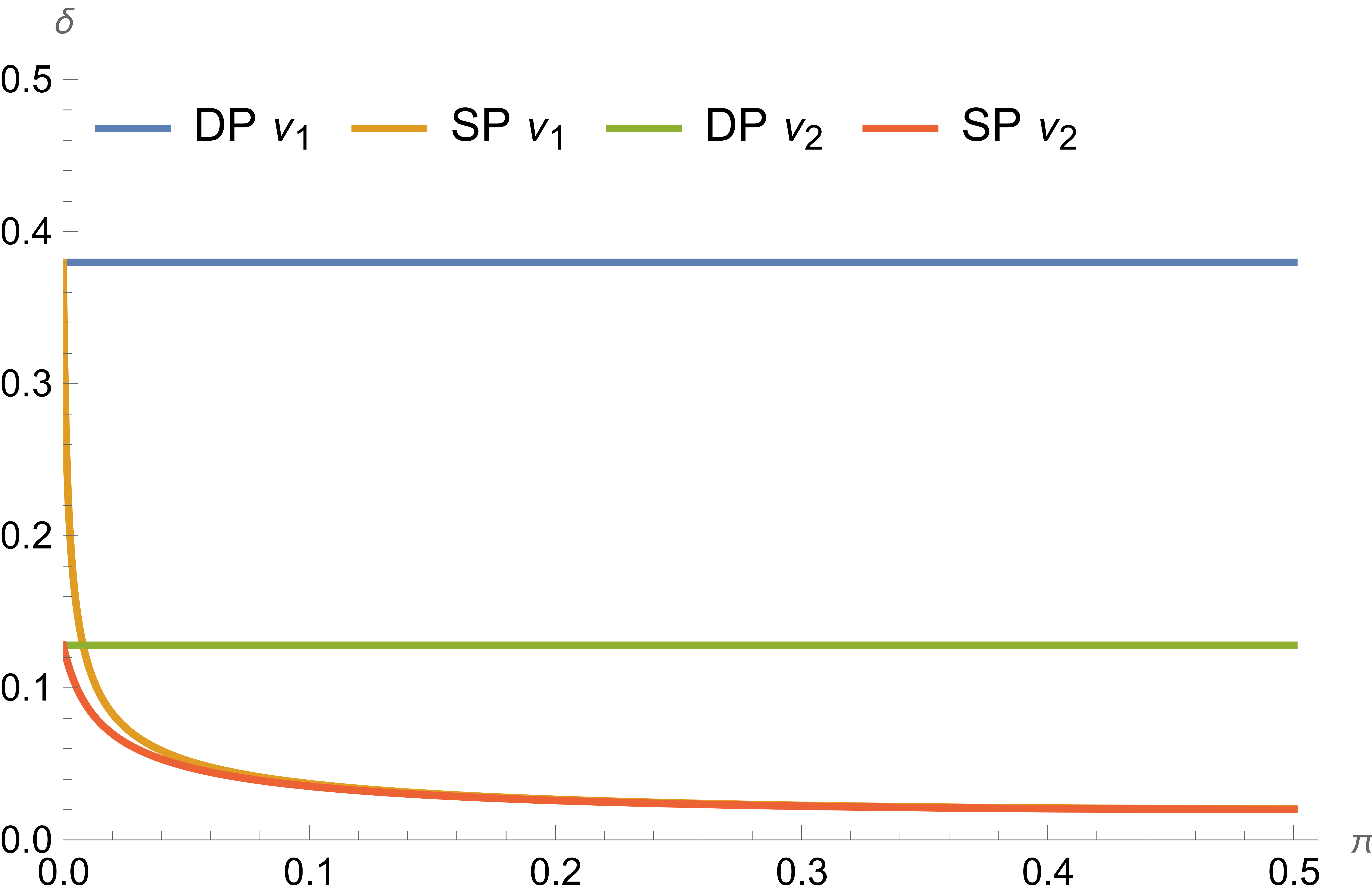
Figure 1: $\delta$ parameter with respect to $\pi$ for noise levels $\nu_{1}=1$ and $\nu_{2}=3$.

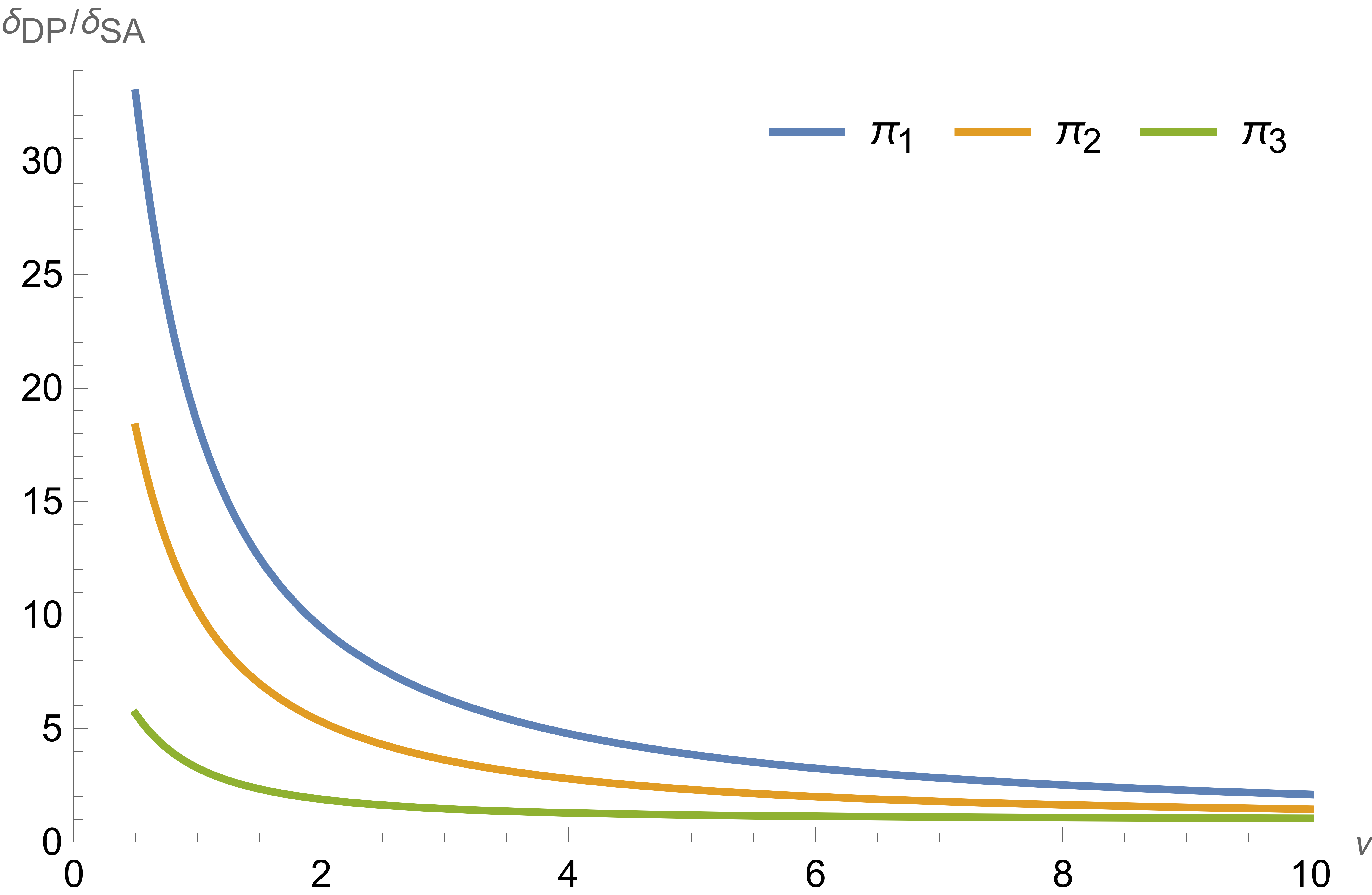
Figure 2: The ratio of the $\delta$ parameters for DP versus SP for different $\pi$-values.

For Gaussian noise, see Fig. 2: with $\nu_{1}$, that means external noise equal to the sensitivity, differential privacy achieves ${\color[rgb]{0,0,0.6}\delta=0.38}$ and ${\color[rgb]{0,0.6,0}\delta=0.128}$ for $\nu_{2}$. In the statistical privacy setting, $\delta$ is much lower and mainly determined by the internal noise if the external noise is moderate. This holds unless $\pi$ gets close to $0$ when the internal noise vanishes. Fig. 2 shows the ratio between the $\delta$-values obtained for these two privacy settings for different values of $\pi$, namely ${\color[rgb]{0,0,0.6}\pi_{1}=0.5}$, ${\color[rgb]{1,0.65,0}\pi_{2}=0.1}$ and ${\color[rgb]{0,0.6,0}\pi_{3}=0.01}$. The $x$-achses gives different strength of external noise where the factor $\nu$ ranges from $1$ to $10$. Even for the maximum $10$ the ratio is significantly larger than $1$. Note that $\pi_{3}$ models a real rare event, where only $1\%$ of all entries are expected to be positive, this means $10$ entries out of $1000$. Adding external noise with $\nu>>1$ degrades the utility of the answer to almost useless.

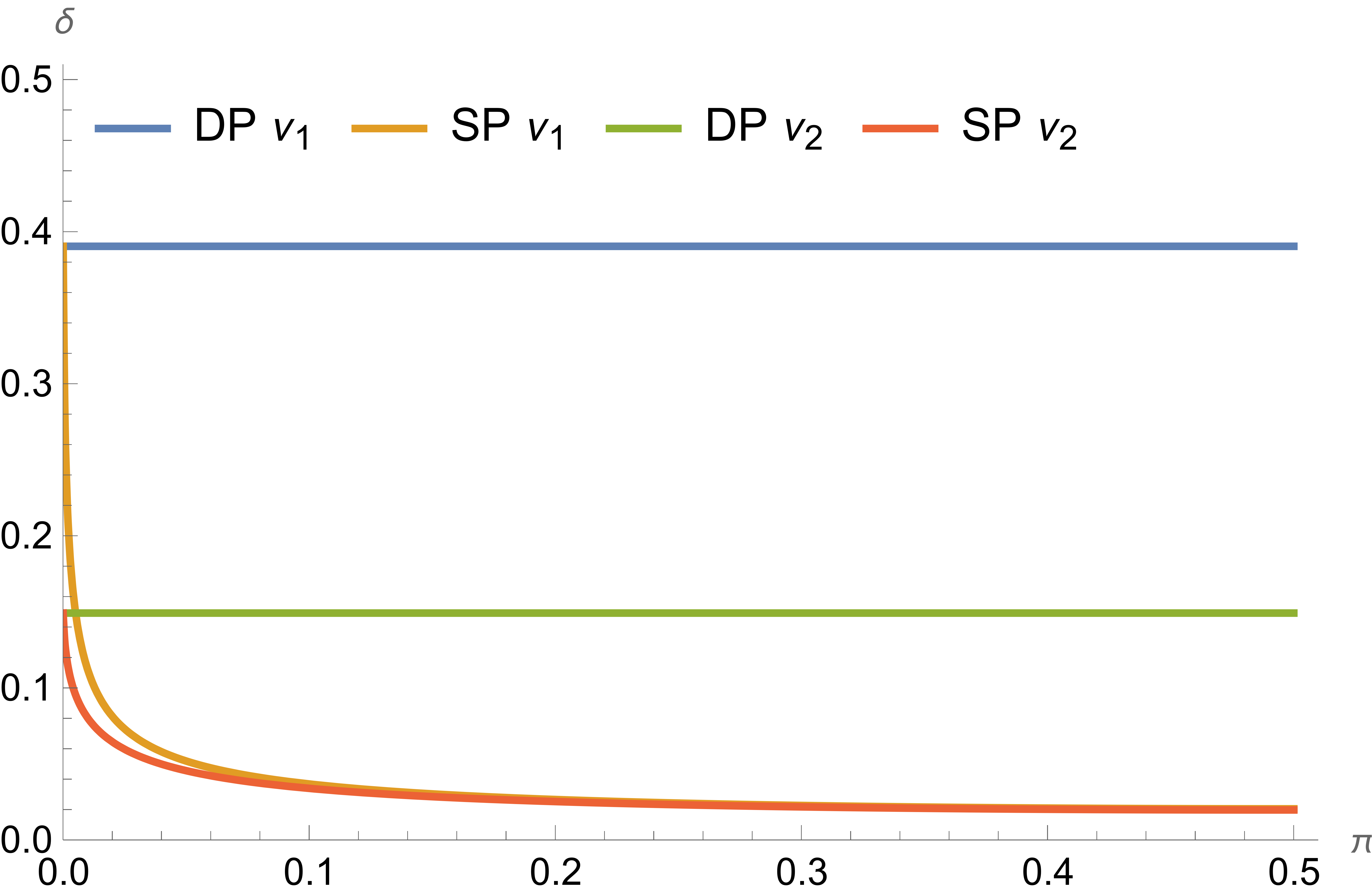
Figure 3: $\delta$ parameter with respect to $\pi$ for noise levels $\nu_{1}=1$ and $\nu_{2}=3$.

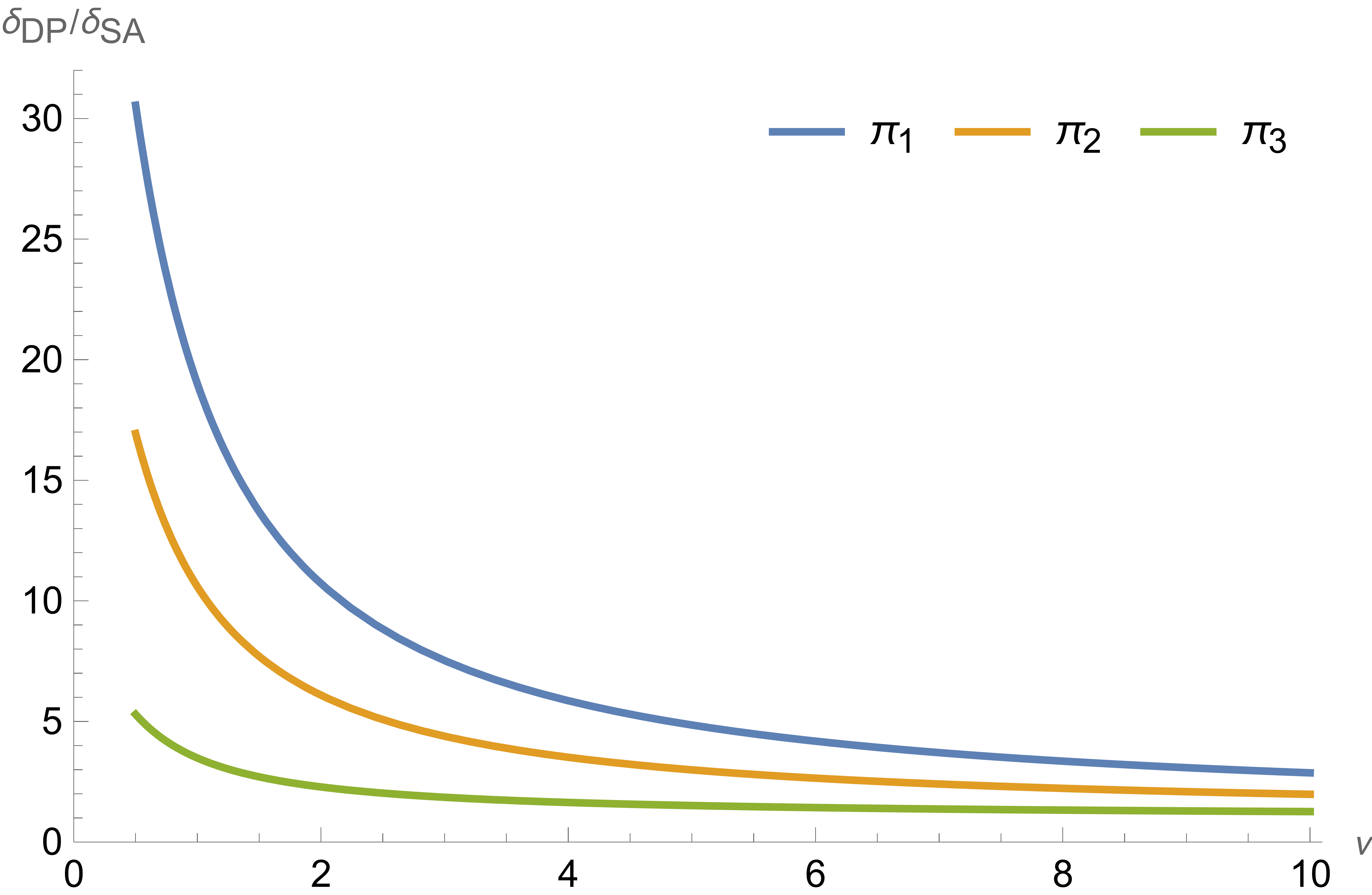
Figure 4: The ratio of the $\delta$ parameters for DP versus SP for different $\pi$-values.

For Laplace noise our computations have used the same parameters. Fig. 4 and 4 show that the results are quite similar. Laplace noise seems to be slightly better suited in the statistical setting. Even for quite small databases of size $n=100$ with much less entropy the internal noise is quite helpful to guarantee privacy as Fig. 6 illustrates. The loss of privacy compared to $n=1000$ is quite small. These results show that internal noise generated by the database distribution has a strong effect on the privacy guarantee obtained even in case of simple property queries.

6 External Noise versus Subsampling for Statistical Privacy

For differential privacy the privacy amplification by subsampling has been studied in [2], for noiseless privacy in [4]. For differential privacy it has been shown that subsampling without replacement with rate $\lambda$ turns a $(\varepsilon,\delta)$-differential privacy mechanism into one with parameters $(\mathop{\rm log}\nolimits\,(1+\lambda(e^{\varepsilon}-1)),\;\lambda\;\delta)$. Since for small $\varepsilon$ the first expression can be approximated by $\mathop{\rm log}\nolimits\,(1+\lambda(e^{\varepsilon}-1))\approx\lambda\;\varepsilon$ this yields a reduction of the privacy parameters by the sampling rate. Small $\lambda$, however, yield high utility loss.

Can the same reduction be achieved in the statistical setting? Here one has to consider that smaller databases provide less entropy. Thus, when the subsampling mechanism generates a database of size $m<<n$ then the base should be the statistical privacy of databases of size $m$. If this were much less than those for size $n$ then this reduces the effect of subsampling. But the previous section has shown that the size reduction does not have a larger effect.

In case of property queries subsampling without replacement generates a hypergeometric distribution that for small sample size can be approximated by a binomial distribution as we have already discussed above. Since a binomial distribution converges to a normal distribution the question arises what is the difference between subsampling and Gaussian noise that generate the same standard deviation of the correct value.

Furthermore, how does a combination of both behave? In the limit as the convolution of two normal distributions one can expect normal distributed distortion with variance being the sum of both variances. But for a precise answer again the same problem arises as for binomial distributions. No exact formula seems to be known for the convolution of a hypergeometric and a normal distribution.

To generate real data on this issue we have done the following computations. For a property query $F^{\pi}$ and $\varepsilon=0.01$ the corresponding $\delta$ is computed given a distortion by Laplace or Gaussian noise, resp. subsampling with $\lambda=0.1$ such that the utility loss is identical for all three cases. The loss is determined by the subsampling rate $\lambda$. Then the strength of the noise is adjusted accordingly to yield the same loss

Figure 5: Comparison of the three mechanisms with respect to the property probability $\pi$

Figure 6: The ratio of the $\delta$ parameters for DP versus SP für $n=100$.

Fig. 6 gives the results with respect to the property probability $\pi$. It shows that Gaussian noise and subsampling practically achieve the same $\delta$-values even in this bounded scenario while Laplace noise is about 20% worse.

Fig. 8 plots the dependency on $\lambda$ for these three distortion techniques for the $\pi$-values $\pi_{1}=0.5$ and $\pi_{2}=0.1$. As above the parameters are chosen in such a way that the utility loss is identical in the three cases. Again the curves of subsampling and Gaussian noise fall together while Laplace noise is always worse. The relative performance of Laplace noise deteriorates with smaller $\lambda$.

7 Conclusion

In this report the privacy risk when accessing a database by property queries has been analyzed for adversaries that know the distribution by which the database is generated. We have named this scenario statistical privacy and shown that good privacy bounds can already be achieved for moderate size databases. They depend on the probability of the property of interest, but are useful unless the probability gets so small that the expected number of positive entries is close to 1.

Figure 7: Results for $n=1000$, $\pi=0.5$ and $\varepsilon=0.1$ the blue curve gives the $\delta$-values for subsampling a database of size $n$ for $\varepsilon^{\prime}=\;\mathop{\rm log}\nolimits\,(1+\lambda(e^{\varepsilon}-1))$; note that $\delta$ increases when decreasing $\lambda$ up to a certain point because $\varepsilon^{\prime}$ gets smaller, the yellow curve shows the values for pure statistical privacy for databases of size $m$ multiplied by $\lambda$

Figure 8: Comparison with respect to the subsampling rate $\lambda$ for $\pi_{1}=0.5$ and $\pi_{2}=0.1$

For analyzing the addition of noise one has to determine the convolution of the noise distribution with the distribution of the query under the database distribution. This is an open mathematical problem for most pairs of distributions.

For distributional privacy there does not exist a general agreement for the choice of $\varepsilon$. Some real applications have used values on the order of 10 or even larger. This does not make sense and would yield a huge privacy leakage in this worst case scenario. When this is still applied to large databases it can only be justified by the condition that an adversary actually does not know almost all entries – thus we are in a statistical privacy setting. The worst case scenario is not appropriate for many applications.

Privacy amplification by subsampling has been well studied for differential privacy. In the statistical setting one has to analyze a mixture distribution which can be quite complex in general. Here we have restricted the query to a binomial distribution. As already discussed subsampling with rate $\lambda$ turns a $(\varepsilon,\delta)$-differential privacy mechanism into one where the parameters are of the form $\left(\;\mathop{\rm log}\nolimits\,(1+\lambda(e^{\varepsilon}-1)),\lambda\;\delta\right)$, which approximately for small $\varepsilon$ can be simplified to $(\lambda\;\varepsilon,\>\lambda\;\delta)$. And this bound is tight.

Does a comparable result hold for statistical privacy? This is not obvious since database of size $m<n$ have less entropy. For property queries one has to compare ${\color[rgb]{0,0,0.6}\delta_{F,{\tt SAMP}(\lambda),\mu_{+},\mu_{-}}(\varepsilon^{\prime})}$ for databases of size $n$ with the pure statistical privacy ${\color[rgb]{1,0.75,0}\delta_{F,\mu_{+},\mu_{-}}(\varepsilon)}$ scaled by the rate $\lambda$. Fig. 8 shows the result of a specific test. Here, subsampling gives even better results. We conjecture that for property queries subsampling never leads to larger $\delta$-values and that this even holds more general, formally:

Let $\nu$ be a probability distribution of entries and $\nu^{n},\;\nu^{m}$ be the product distribution of $\nu$ for databases of size $n$, resp. $m$. If $F$ is a symmetric query that is $(\varepsilon,\delta)$–pure statistical private for databases of size $m$ with distribution $\nu^{m}$ then $(F,M_{{\tt SAMP}})$ with selection property $\lambda=n/m$ is $(\;\mathop{\rm log}\nolimits\,(1+\lambda(e^{\varepsilon}-1)),\lambda\;\delta)$–statistical private for databases of size $n$ with distribution $\nu^{n}$.

Further questions include other subsampling types, for example with replacement. We have shown that for additive noise the utility loss is equal to the variance of the noise in the statistical setting. Given a maximal acceptable utility loss Laplace noise seems to perform worse than Gaussian noise in general. This should be examined in more detail.

References

- [1] Abadi, M., Chu, A., Goodfellow, I., McMahan, H., Mironov, I., Talwar, K., Zhang, L.: Deep learning with differential privacy. In: Proc. ACM CC. pp. 308–318 (2016)
- [2] Balle, B., Barthe, G., Gaboardi, M.: Privacy profiles and amplification by subsampling. J. Privacy and Confidentiality 10(1) (2020). https://doi.org/10.29012/jpc.726
- [3] Bassily, R., Groce, A., Katz, J., Smith, A.: Coupled-worlds privacy: Exploiting adversarial uncertainty in statistical data privacy. In: Proc. 54. FOCS. p. 439–448 (2013). https://doi.org/10.1109/FOCS.2013.54
- [4] Bhaskar, R., Bhowmick, A., Goyal, V., Laxman, S., Thakurta, A.: Noiseless database privacy. In: Proc. ASIACRYPT 2011. pp. 215–232. Springer LNCS 7073 (2011)
- [5] Desfontaines, D.: A list of real-world uses of differential privacy. https://desfontain.es/blog/real-world-differential-privacy.html (2021)
- [6] Desfontaines, D., Mohammadi, E., Krahmer, E., Basin, D.: Differential privacy with partial knowledge (2020)
- [7] Desfontaines, D., Pejo, B.: Sok: Differential privacies – a taxonomy of differential privacy variants and extensions (2022)
- [8] Dwork, C., McSherry, F., Nissim, K., Smith, A.: Calibrating noise to sensitivity in private data analysis. J. Privacy and Confidentiality 3, 17–51 (2016)
- [9] Dwork, C., Roth, A.: The algorithmic foundations of differential privacy. Foundations and Trends® in Theoretical Computer Science 9(3–4), 211–407 (2014). https://doi.org/10.1561/0400000042
- [10] Imola, I., Chaudhuri, K.: Privacy amplification via Bernoulli sampling. In: Proc. 38. Int. Conf. on Machine Learning (2021)
- [11] Joseph, N., David, D.: Differential privacy: Future work & open challenges. https://www.nist.gov/blogs/cybersecurity-insights/differential-privacy-future-work-open-challenges (1 2022), an official website of the United States government
- [12] Kifer, D., Lin, B.: An axiomatic view of statistical privacy and utility. J. Privacy and Confidentiality 4, 5–49 (2012)
- [13] Meiser, S.: Approximate and probabilistic differential privacy definitions. Cryptology ePrint Archive (2018)
- [14] Mironov, I.: Renyi differential privacy. In: Proc. 30. Computer Security Foundations Symposium (2017)
- [15] Sommer, D., Meiser, S., Mohammadi, E.: Privacy loss classes: The central limit theorem in differential privacy. In: Proc. Privacy Enhancing Technologies Symposium. vol. 2019 (2), pp. 245–269 (2019). https://doi.org/10.2478/popets-2019-0029
- [16] Steinke, T.: Composition of differential privacy and privacy amplification by subsampling. In: arXiv:2210.00597 (2022)
- [17] Wang, Y., Balle, B., Kasiviswanathan, S.: Subsampled Renyi differential privacy and analytical moments accountant. In: Proc. 22. AISTATS (2019)