The Deimginarity Cost of Quantum States
Abstract
Here we address a task denoted as deimaginarity, which is to transform a state into a real state with the aid of random covariant-free unitary operations. We consider the minimum cost of randomness required for deimaginarity in the scenario of infinite copies and sufficiently small error, and we prove that the deimaginarity cost of a state is equal to its regularized relative entropy of imaginarity, which can be seen as an operational interpretation of the relative entropy of imaginarity.
pacs:
03.65.Ud, 03.67.MnI Introduction
Quantum resource theories provide a fancy view to address the properties of quantum systems and present their applications in various quantum information tasks gour2015resource ; chitambar2019quantum ; gour2024resources . Among them, entanglement is one of the most fundamental resources horodecki2009quantum ; friis2019entanglement ; erhard2020advances . By consuming entanglement, varieties of protocols can be implemented that are impossible in the view of classical information theory, such as dense coding bennett1992communication , and quantum telecommunication bennett1993teleporting . Recently, many other quantum resources have been developed,such as coherence streltsov2017colloquium ; hu2018quantum , asymmetry marvian2012symmetry , magic howard2017application ; veitch2014resource , nonlocality brunner2014bell , steering cavalcanti2016quantum ; uola2020quantum and imaginarity hickey2018quantifying .
Due to the postulates of quantum mechanics Nielsen_Chuang_2010 , quantum information theory builds on the complex field. Many significant results showed the necessity and values of the imaginary part stueckelberg1960quantum ; wootters2014rebit ; renou2021quantum ; chiribella2023positive . Nevertheless, until recent years, imaginarity has been studied in the view of resource theory hickey2018quantifying ; wu2021resource ; wu2021operational ; kondra2023real ; wu2024resource ; zhang2024broadcasting . A fundamental problem of resource theory is how to quantify the resourcefulness of a quantum state hickey2018quantifying ; kondra2023real ; xue2021quantification . Among the commonly used quantifiers in the imaginarity resource, the method to quantify the imaginarity in terms of the relative entropy, the relative entropy of imaginarity, is considered in xue2021quantification . It is a strong imaginarity monotone and additive xue2021quantification . However, as far as I know, the operational interpretation of the relative entropy of imaginarity (REI) is unknown.
In this paper, we address the above problem by analyzing a task which is to transform a state into a real state with the aid of random free unitary operators. We consider the above task in the scenarios of infinite copies and vanishing errors, and present the minimum cost of randomness per copy to deimaginarity is equal to the REI. This task has been considered in the resource theory of multipartite correlations groisman2005quantum , entanglement berta2018disentanglement , coherence singh2015erasing , asymmetry wakakuwa2017symmetrizing , non-markovianity 9214470 , and dynamical resources liu2019resource .
This paper is organized as follows. In Sec. II, we review the definitions, properties, and measures of quantums state in terms of the imaginarity resource. In Sec. III, we present the definition of the deimaginarity cost of a state and the main result of this article. In Sec. IV, we end with a conclusion.
II Preliminary Knowledge
In this section, we recall the definitions of the imaginary of quantum states. We also review some quantifiers of the imaginary resource of quantum states.
II.1 The Resource Theory of Imaginarity
Here we consider a quantum system described by with finite dimensions. We denote as the set of linear operators of and as the set of states on Before reviewing the resource theory of imaginarity hickey2018quantifying , we fix an orthonormal reference basis of with its dimension .
In the imaginarity theory, the real states are called the free states, which is the set of a quantum state with a real density matrix,
| (1) |
here In this manuscript, we denote the set of all real density matrices as As all density matrices are Hermitian, a state if and only if Due to the definitions of is convex and affine. Besides, the set depends on the orthonormal reference basis .
Next we present the formulation of the free operations of this resource theory. In general, quantum channels can be represented by a set of Kraus operations with . The free operations of imaginarity theory can be specified by the Kraus operations with , here and takes over all the elements in the basis . Due to the properties of free operations of imaginarity theory, the real operations cannot creat imginarity from real states.
Assume is a unitary operator acting on the system , is RNG if and only , here is a real orthogonal operator. Let . When satisfies , is covariant. Next if is covariant, and is a free state
that is, . Hence, is a free state. That is, a covariant-free unitary operation cannot transform a free state into a resourceful state.
Before we introduce the process of deimaginarity of a generic state, we present the process of deimaginarity of the maximally resourceful state, . The deimaginary process can be achieved by two unitary operators and with equal probability,
Note that , and That is, by the application of two covariant unitary operations with equal probability, we could erase the imaginarity of the maximally resourceful state. The above effects can also be implemented for a dimensional quantum system. Let is a -dimensional system, any state acting on can be decomposed as
here is a real symmetric quantum state, and is a real anti-symmetric state. Moreover, there exists a real horn such that
where For a real orthogonal matrix , we have
| (2) |
Besides, for a state of two-dimensional systems, we have
| (3) |
That is, there always exists an ensemble of covariant-free unitaries to erase the imaginarity of a quantum state.
Next we present the resource theory of imaginarity of the composite systems. Assume is a Hilbert space with reference orthogonal basis , let be a system composed of duplicates of with reference orthogonal basis . A state acting on is free in terms of the imaginarity resource if and only if , here is with respect to the basis . As is a composite space composed of duplicates of , the transpose operator of can be seen as , here is the transpose operator of with repect to the reference basis
II.2 Relative Entropy of the Resource Theory of Imaginarity
To quantify the imaginarity of a quantum state, Xue considered a quantifier called the relative entropy of imaginarity (REI) of a quantum state xue2021quantification ,
| (4) |
where the minimum takes over all the real states , and Moreover, the REI can be written as
| (5) |
where , and . The REI is additive.
Up to now, there exists few results on the REI, , here we present a direct operational meaning of the REI.
III Main Results
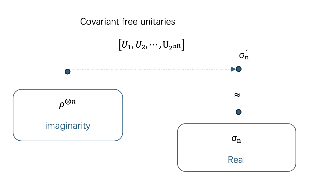
Assume is a state of a system with finite dimensions. A basic task is to transform a state to a real state by applying covariant-free unitary operations randomly. A fundamental problem is to minimize the cost of randomness to make the imaginary state free.
Definition 1
Assume is a state of with finite dimensions. A rate is denoted to be achievable to make free with respect to the reference basis of if, there exists a large such that there exists a free state and a set of real ortthogonal operators with such that
here
The deimaginarity cost of a state with respect to the reference basis is
Here the schematic diagram of the task of deimaginarity cost of a state is plotted in Fig 1.
The main result of this article is to present the analytical representation of the deimaginarity cost of a state , .
Theorem 2
Assume is a state acting on the Hilbert space then
The proof of this theorem is placed in Sec. VI
IV Conclusion
In this paper, we considered the task of deimaginarity, and analyzed the minimal cost of randomness needed to make a state real. Particularly, we addressed the transformation task in the scenarios of an asymptotic limit of infinite copies and vanishing error, and we showed the minimum cost of the randomness for a state to make it real is equal to the regularized relative entropy of imaginarity of the state. At last, it would be meaningful to study the task in terms of other resources of some quantum system, such as steering cavalcanti2016quantum ; uola2020quantum and contextuality budroni2022kochen ; pavicic2023quantum .
V Acknowledgement
X. S. was supported by the National Natural Science Foundation of China (Grant No. 12301580).
References
- (1) G. Gour, M. P. Muller, V. Narasimhachar, R. W. Spekkens, and N. Y. Halpern, “The resource theory of informational nonequilibrium in thermodynamics,” Physics Reports, vol. 583, pp. 1–58, 2015.
- (2) E. Chitambar and G. Gour, “Quantum resource theories,” Reviews of modern physics, vol. 91, no. 2, p. 025001, 2019.
- (3) G. Gour, “Resources of the quantum world,” arXiv preprint arXiv:2402.05474, 2024.
- (4) R. Horodecki, P. Horodecki, M. Horodecki, and K. Horodecki, “Quantum entanglement,” Reviews of modern physics, vol. 81, no. 2, pp. 865–942, 2009.
- (5) N. Friis, G. Vitagliano, M. Malik, and M. Huber, “Entanglement certification from theory to experiment,” Nature Reviews Physics, vol. 1, no. 1, pp. 72–87, 2019.
- (6) M. Erhard, M. Krenn, and A. Zeilinger, “Advances in high-dimensional quantum entanglement,” Nature Reviews Physics, vol. 2, no. 7, pp. 365–381, 2020.
- (7) C. H. Bennett and S. J. Wiesner, “Communication via one-and two-particle operators on einstein-podolsky-rosen states,” Physical review letters, vol. 69, no. 20, p. 2881, 1992.
- (8) C. H. Bennett, G. Brassard, C. Crepeau, R. Jozsa, A. Peres, and W. K. Wootters, “Teleporting an unknown quantum state via dual classical and einstein-podolsky-rosen channels,” Physical review letters, vol. 70, no. 13, p. 1895, 1993.
- (9) A. Streltsov, G. Adesso, and M. B. Plenio, “Colloquium: Quantum coherence as a resource,” Reviews of Modern Physics, vol. 89, no. 4, p. 041003, 2017.
- (10) M.-L. Hu, X. Hu, J. Wang, Y. Peng, Y.-R. Zhang, and H. Fan, “Quantum coherence and geometric quantum discord,” Physics Reports, vol. 762, pp. 1–100, 2018.
- (11) I. Marvian Mashhad, “Symmetry, asymmetry and quantum information,” 2012.
- (12) M. Howard and E. Campbell, “Application of a resource theory for magic states to fault-tolerant quantum computing,” Physical review letters, vol. 118, no. 9, p. 090501, 2017.
- (13) V. Veitch, S. H. Mousavian, D. Gottesman, and J. Emerson, “The resource theory of stabilizer quantum computation,” New Journal of Physics, vol. 16, no. 1, p. 013009, 2014.
- (14) N. Brunner, D. Cavalcanti, S. Pironio, V. Scarani, and S. Wehner, “Bell nonlocality,” Reviews of modern physics, vol. 86, no. 2, pp. 419–478, 2014.
- (15) D. Cavalcanti and P. Skrzypczyk, “Quantum steering: a review with focus on semidefinite programming,” Reports on Progress in Physics, vol. 80, no. 2, p. 024001, 2016.
- (16) R. Uola, A. C. Costa, H. C. Nguyen, and O. Guhne, “Quantum steering,” Reviews of Modern Physics, vol. 92, no. 1, p. 015001, 2020.
- (17) A. Hickey and G. Gour, “Quantifying the imaginarity of quantum mechanics,” Journal of Physics A: Mathematical and Theoretical, vol. 51, no. 41, p. 414009, 2018.
- (18) M. A. Nielsen and I. L. Chuang, Quantum Computation and Quantum Information: 10th Anniversary Edition. Cambridge University Press, 2010.
- (19) E. C. Stueckelberg, “Quantum theory in real hilbert space,” Helv. Phys. Acta, vol. 33, no. 727, p. 458, 1960.
- (20) W. K. Wootters, “The rebit three-tangle and its relation to two-qubit entanglement,” Journal of Physics A: Mathematical and Theoretical, vol. 47, no. 42, p. 424037, 2014.
- (21) M.-O. Renou, D. Trillo, M. Weilenmann, T. P. Le, A. Tavakoli, N. Gisin, A. Acin, and M. Navascues, “Quantum theory based on real numbers can be experimentally falsified,” Nature, vol. 600, no. 7890, pp. 625–629, 2021.
- (22) G. Chiribella, K. R. Davidson, V. I. Paulsen, and M. Rahaman, “Positive maps and entanglement in real hilbert spaces,” in Annales Henri Poincare, vol. 24, no. 12. Springer, 2023, pp. 4139–4168.
- (23) K.-D. Wu, T. V. Kondra, S. Rana, C. M. Scandolo, G.-Y. Xiang, C.-F. Li, G.-C. Guo, and A. Streltsov, “Resource theory of imaginarity: Quantification and state conversion,” Physical Review A, vol. 103, no. 3, p. 032401, 2021.
- (24) ——, “Operational resource theory of imaginarity,” Physical Review Letters, vol. 126, no. 9, p. 090401, 2021.
- (25) T. V. Kondra, C. Datta, and A. Streltsov, “Real quantum operations and state transformations,” New Journal of Physics, vol. 25, no. 9, p. 093043, 2023.
- (26) K.-D. Wu, T. V. Kondra, C. M. Scandolo, S. Rana, G.-Y. Xiang, C.-F. Li, G.-C. Guo, and A. Streltsov, “Resource theory of imaginarity in distributed scenarios,” Communications Physics, vol. 7, no. 1, p. 171, 2024.
- (27) Z. Zhang, N. Li, and S. Luo, “Broadcasting of imaginarity,” Physical Review A, vol. 110, no. 5, p. 052439, 2024.
- (28) S. Xue, J. Guo, P. Li, M. Ye, and Y. Li, “Quantification of resource theory of imaginarity,” Quantum Information Processing, vol. 20, pp. 1–20, 2021.
- (29) B. Groisman, S. Popescu, and A. Winter, “Quantum, classical, and total amount of correlations in a quantum state,” Physical Review A—Atomic, Molecular, and Optical Physics, vol. 72, no. 3, p. 032317, 2005.
- (30) M. Berta and C. Majenz, “Disentanglement cost of quantum states,” Physical Review Letters, vol. 121, no. 19, p. 190503, 2018.
- (31) U. Singh, M. N. Bera, A. Misra, and A. K. Pati, “Erasing quantum coherence: an operational approach,” arXiv preprint arXiv:1506.08186, 2015.
- (32) E. Wakakuwa, “Symmetrizing cost of quantum states,” Physical Review A, vol. 95, no. 3, p. 032328, 2017.
- (33) ——, “Communication cost for non-markovianity of tripartite quantum states: A resource theoretic approach,” IEEE Transactions on Information Theory, vol. 67, no. 1, pp. 433–451, 2021.
- (34) Z.-W. Liu and A. Winter, “Resource theories of quantum channels and the universal role of resource erasure,” arXiv preprint arXiv:1904.04201, 2019.
- (35) R. A. Horn and J. C. R., Matrix analysis. Cambridge University Press, 2012.
- (36) C. Budroni, A. Cabello, O. Guhne, M. Kleinmann, and J. Larsson, “Kochen-specker contextuality,” Reviews of Modern Physics, vol. 94, no. 4, p. 045007, 2022.
- (37) M. Pavicic, “Quantum contextuality,” Quantum, vol. 7, p. 953, 2023.
- (38) M. Fannes, “A continuity property of the entropy density for spin lattice systems,” Communications in Mathematical Physics, vol. 31, pp. 291–294, 1973.
- (39) M. Thomas and A. T. Joy, Elements of information theory. Wiley-Interscience, 2006.
- (40) A. Winter, “Coding theorem and strong converse for quantum channels,” IEEE Transactions on Information Theory, vol. 45, no. 7, pp. 2481–2485, 1999.
- (41) R. Ahlswede and A. Winter, “Strong converse for identification via quantum channels,” IEEE Transactions on Information Theory, vol. 48, no. 3, pp. 569–579, 2002.
VI Appendix
VI.1 Proof of Theorem 2
Here we prove Theorem 2 separablely, first we prove the converse part first, then we show . Combing the proof of the both parts, we finish the proof of Theorem 2.
VI.1.1 Converse Part
Assume , for any and sufficiently large , there exists a free state and a set of unitaries such that
| (A.1) |
here satisfies Next let ,as , ,
| (A.2) | ||||
| (A.3) | ||||
| (A.4) | ||||
| (A.5) |
here the first inequality is due to the triangle inequality of the -norm, the equality is due to that is free, the second inequality is due to the contractive property of the trace-preserving quantum operations under the -norm.
Assume is an ancillary system with dimension , and ,
Next let is a purification of let
then
| (A.6) |
here the second inequality is due to the subadditivity of von Neumann entropy , the second equality follows from
Next due to the inequality (A.5) and the Fannes inequality fannes1973continuity , we have
| (A.7) |
here satisfies Then due to the concavity of the von Neumann entropy, we have
| (A.8) | ||||
| (A.9) | ||||
| (A.10) |
here the first inequality is due to the concavity of , the second inequality is due to that is covariant-free and Lemma 6.
As the above inequality holds for all and arbitrarily small , we finish the proof of the converse part.
VI.1.2 Direct Part
In this subsection, we will present the proof of the following inequality,
The method of this proof is similar to the one shown in groisman2005quantum ; wakakuwa2017symmetrizing . The preliminary knowledge needed here are placed in Sec. VI.2.
Assume is the -typical subspacces with respect to . is the projection onto the space . Due to the properties of -typical subspace presented in Sec. VI.2, for any there exists a large such that
| (A.13) | |||
| (A.14) |
Based on and the Gentle Measurement Lemma 3, we have
| (A.15) |
Here we denote as the dimension of , then
The last inequality is due to the additivity of for product states and Lemma 7.
Assume is an ensemble of the covariant-free unitary operators such that for any state acting on the Hilbert space , , here is the identity acting on the space . Hence, we have
| (A.16) |
here
Next let us denote as random operators with its distribution . Let Based on (A.14), we have
| (A.17) |
hence . Let
then we have the minimum nonzero eigenvalue of is bounded by
| (A.18) |
If are i.i.d. , then by Lemma 5, we have
Denote , the right hand side of the above inequality is nonzero when is sufficiently large. Then there exists such that
| (A.19) |
here is real, hence, we have
here the first inequality is due to the triangle inequality of the -norm, the second inequality is due to (A.15) and (A.19). Note that and in the above proof can be chosen arbitrarily small, is achievable if , hence, we finish the proof.
VI.2 Mathematical Tools
In this subsection, we present necessary knowledge needed in the proof of the first two subsections of this appendix.
VI.2.1 Typical Sequences and Subspaces
Next we recall the definitions and properties of typical subspaces thomas2006elements . Assume is a discrete random variable with finite alphabet and when . A sequence is denoted as -typical with respect to if it owns the following property,
where is the Shannon entropy of . The set of all -typical sequences is called the -typical set, which is denoted as . The set owns the following property,
Moreover, based on the wek law of large numbers, for arbitrary positive , , and sufficiently large .
Assume is a state acting on the system , The -typical subspace with respect to is
where is the -typical set with respect to . Assume is the projection of , then
For any and sufficiently large , we have
VI.2.2 Necessary Lemmas
Lemma 3 (Gentle Measurement Lemma)
winter1999coding Assume is a density matrix with acting on a finite dimensional system, then for any such that and , we have
Lemma 4 (Fannes Inequality)
Lemma 5 (Operator Chernoff Bound)
ahlswede2002strong Assume are i. i. d. random variables taking values in the operator interval with expectation , then for , and denote
Lemma 6
Assume , and is a covariant-free unitary operation, then
Proof.
Lemma 7
Assume is a state, then
| (A.24) |
Proof.
As , then each eigenvalue of is nonnegative. Let is arbitrary eigenvalue of with its corresponding eigenvector is
that is is also the eigenvalue of . Hence, Due to the concativity of we have