Algebraic Lagrangian cobordisms, flux and the Lagrangian Ceresa cycle

Abstract.

We introduce an equivalence relation for Lagrangians in a symplectic manifold known as algebraic Lagrangian cobordism, which is meant to mirror algebraic equivalence of cycles. From this we prove a symplectic, mirror-symmetric analogue of the statement “the Ceresa cycle is non-torsion in the Griffiths group of the Jacobian of a generic genus $3$ curve”. Namely, we show that for a family of tropical curves, the Lagrangian Ceresa cycle, which is the Lagrangian lift of their tropical Ceresa cycle to the corresponding Lagrangian torus fibration, is non-torsion in its oriented algebraic Lagrangian cobordism group. We proceed by developing the notions of tropical (resp. symplectic) flux, which are morphisms from the tropical Griffiths (resp. algebraic Lagrangian cobordism) groups.

1. Introduction

In a smooth projective variety, studying and comparing the different equivalence relations between algebraic cycles can shed light on a wealth of interesting geometric phenonema. A chief example is that of the Ceresa cycle of a curve, which is a $1$-cycle living its Jacobian, and provided the first instance of a cycle which was shown to be homologically, but not algebraically, trivial [Cer83]. This discrepancy between homological and algebraic equivalence is encoded in the Griffiths group of the variety. Our aim is to propose a symplectic counterpart to this group and use it to exhibit, through an $SYZ$ picture, a symplectic manifestation of the fact that the Ceresa cycle is not algebraically trivial.

While we survey below how the (cylindrical) cobordism group of a symplectic manifold $(X,\omega)$ is known to be closely related to the Chow groups of its mirror, a candidate mirror to its Griffiths groups (that is, the quotient of the Chow groups by algebraic equivalence) has, to the best of our knowledge, not yet appeared in the literature. We propose such a mirror by introducing an equivalence relation which we call algebraic Lagrangian cobordism on the set of suitable Lagrangians in a symplectic manifold, and from this we define the algebraic Lagrangian cobordism group of $(X,\omega)$, $algCob(X)$.

The predicted relation between the Lagrangian cobordism group of a symplectic manifold $X$, denoted $\mathcal{C}ob(X)$, and the Chow groups of its mirror $\check{X}$, was first brought to light in the context of SYZ fibrations by Sheridan–Smith in [SS21]. Their constructions rely on the following observation. Let $B$ be a tropical torus, $Z_{1}$ and $Z_{2}$ be tropical cycles in $B$, and consider the Lagrangian torus fibration

$$X(B):=T^{*}B/T^{*}_{\mathbb{Z}}B\longrightarrow B.$$

A rational equivalence between $Z_{1}$ and $Z_{2}$, if it admits a Lagrangian lift to $X(B\times\mathbb{R})\cong X(B)\times\mathbb{C}^{*}$, defines a (cylindrical) Lagrangian cobordism between the Lagrangian lifts $L_{1}$ and $L_{2}$ of $Z_{1}$ and $Z_{2}$.

From the perspective of homological mirror symmetry, this correspondence can be formulated as follows. An equivalence of triangulated categories

$$\mathcal{D}^{\pi}\mathcal{F}uk(X)\cong D^{b}Coh(Y)$$

would in particular imply an isomorphism

$$K_{0}(D^{\pi}\mathcal{F}uk(X))\cong K_{0}(D^{b}Coh(Y))$$

between their Grothendieck groups. On the right-hand side, assuming $Y$ is smooth projective, it is known that

$$K_{0}(D^{b}Coh(Y))_{\mathbb{Q}}\cong K_{0}(Coh(Y))_{\mathbb{Q}}\cong CH_{*}(Y)_{\mathbb{Q}},$$

where $CH_{*}(Y)$ is the Chow ring of $Y$ and the second isomorphism is given by the Chern character map $ch$; see [Gil05, Section 2.3]. On the left-hand side, Biran$-$Cornea have shown in [BC13, BC14] that $K_{0}(D\mathcal{F}uk(X))$ is closely related to (the appropriate flavour of) the Lagrangian cobordism group $\mathcal{C}ob(X)$, which we define in section 2. More precisely, Lagrangian cobordisms yield triangle decompositions in the Fukaya category, therefore there is a surjective morphism

$$\mathcal{C}ob(X)\longrightarrow K_{0}(\mathcal{F}uk(X)).$$

In some cases, we know this to be an isomorphism [Hau15, Muñ24, Rat23], and it is interesting to note that the first two of these examples rely on a proof of homological mirror symmetry hence on understanding the mirror Chow groups. Purely symplectically, this line of questions amounts to uncovering which triangle decompositions in $\mathcal{F}uk(X)$ can be realised geometrically by Lagrangian cobordisms.

For symplectic topologists, one of the motivations for studying the groups $\mathcal{C}ob(X)$ associated to a symplectic manifold $X$ is that Lagrangian cobordism provides a coarser equivalence relation than Hamiltonian isotopy (see Example 2.2). Therefore understanding $\mathcal{C}ob(X)$ ought to be simpler than the famously hard problem of classifying Lagrangians in $X$ up to Hamiltonian isotopy. Nevertheless, currently there are only few instances in which these cobordism groups are fully understood. In dimension two, Arnold computed $\mathcal{C}ob(T^{*}S^{1})$ using flux arguments [Arn80] (see Section 2), then Haug used similar techniques to compute $\mathcal{C}ob(T^{2})$ [Hau15]. Rathael-Fournier computed Lagrangian cobordisms groups for higher-genus surfaces through a different approach [Rat23], namely using the action of the mapping class group to obtain generators following work of Abouzaid [Abo08]. The first computation for compact symplectic manifolds in dimension four was carried out by Muñiz-Brea in [Muñ24] for symplectic bielliptic surfaces, restricting to tropical Lagrangians. In the non-compact case, Bosshard studies $\mathcal{C}ob(X)$ when $X$ is a Liouville manifold, and computes these for non-compact Riemann surfaces of finite type [Bos24]. Here again, we have omitted information about the exact flavour of cobordism group considered in each of these cases.

In light of the observations above, it is natural to wonder whether one could further our understanding of Lagrangian cobordism groups by translating interesting examples about Chow cycles to the symplectic realm. Our main result achieves this; we exhibit an example of a nullhomologous Lagrangian $3$-manifold, namely the Lagrangian Ceresa cycle inside a symplectic $6$-torus, which is non-zero (and even non-torsion) in its Lagrangian cobordism group.

Theorem 1.1.

The Lagrangian Ceresa cycle $L-L^{-}$ has infinite order in $\mathcal{C}ob^{or}(X)$.

Here $X$ is a $6$-torus endowed with a symplectic structure constructed in Section 6; see Section 7 for a more precise version of this statement.

This result mirrors a classical algebraic story of the Ceresa cycle. Given an algebraic curve $C$, its Ceresa cycle is a homologically trivial $1$-cycle in the Jacobian $J(C)$, which we denote by $C-C^{-}\in CH_{1}(J(C))_{hom}$. It has been the subject of extensive study since Ceresa proved that for a generic genus $3$ curve, it provides an example of a homologically trivial cycle which is not algebraically trivial. More precisely, letting

$$\text{Griff}_{1}(J(C)):=CH_{1}(J(C))_{hom}/\sim$$

be the Griffiths group, with $\sim$ denoting algebraic equivalence, Ceresa proves the following:

Theorem 1.2 ([Cer83]).

For a generic genus $3$ curve, $C-C^{-}$ has infinite order in $\text{Griff}_{1}(J(C))$.

Let us note that Theorem 1.1 is not exactly mirror to Ceresa’s result 1.2, but rather to the weaker statement that for a generic genus $3$ curve, $C-C^{-}$ has infinite order in $CH_{1}(J(C))_{hom}$. This is where algebraic Lagrangian cobordisms come into play. The reason that the equivalence relation mirror to algebraic - rather than rational - equivalence is less straightforward, is that mirrors to higher genus curves are vastly complicated objects. An insight by which one can circumvent this difficulty is that a curve can be embedded into its Jacobian. From this perspective one can equivalently define algebraically equivalent cycles as cycles living in some family over a abelian variety. Then a candidate mirror equivalence relation for Lagrangians in $(X,\omega)$ would be to say two Lagrangians $L$ and $L^{\prime}$ are algebraically Lagrangian cobordant if they live in some Lagrangian family over a symplectic polarised torus; see Section 3. We call the group of suitable Lagrangians modulo the equivalence relation generated by algebraic Lagrangian cobordisms the algebraic Lagrangian cobordism group of the symplectic manifold, which we denote $algCob(X,\omega)$ or simply $algCob(X)$. A Lagrangian cobordism between finite sets of Lagrangians implies in particuar that they are algebraically Lagrangian cobordant, so there is a natural projection map

$$\mathcal{C}ob(X)\stackrel{{\scriptstyle\pi}}{{\longrightarrow}}algCob(X).$$

With this set up, Theorem 1.1 can be upgraded to

Theorem 1.3.

The Lagrangian Ceresa cycle $L-L^{-}$ has infinite order in $algCob^{or}(X)$.

Our proof relies on the tropical version of Ceresa’s statement 1.2, which is due to Zharkov [Zha13]. To a tropical curve $C$, one can similarly associate its tropical Ceresa cycle $C-C^{-}\in CH_{1}(J(C))^{trop}_{hom}$. Zharkov proves

Theorem 1.4.

[Zha13, Theorem 3] For a generic genus $3$ tropical curve of type $K4$, $C$ and $C^{-}$ are not algebraically equivalent.

A tropical curve of type $K4$ is represented in Figure 2, and is only one of five types of generic genus $3$ tropical curves. The other four are drawn in Figure 7. It distinguishes itself as the only non-hyperelliptic type; this is explained and discussed in Section 8.1. The fact that Ceresa’s classical statement does not translate for other generic types can be understood as a consequence of the failure of the tropical Torelli theorem.

Zharkov’s proof of Theorem 1.2 introduces a specific instance of what we refer to in this paper as tropical flux, namely a morphism

$$\Theta:\text{Griff}_{1}^{trop}(J(C))\longrightarrow\mathbb{R}/\mathcal{P},$$

where $\mathcal{P}$ is a finitely generated subgroup in $\mathbb{R}$. This morphism is given by integrating a tropical differential form $\Omega_{0}$, called the determinantal form, over a $2$-chain bounding cycles in $\text{Griff}_{1}^{trop}(J(C))$. The lattice $\mathcal{P}$ is simply given by the periods of $\Omega_{0}$. One can then conclude by proving that, for generic $C$,

$$m\cdot\Theta(C-C^{-})\neq 0\mod\mathcal{P}$$

for any $m\in\mathbb{Z}$. In Section 5.3 we extend this to aribtrary $k$-cycles in a tropical torus $B$ by defining morphisms

$$\Theta_{k}:\text{Griff}_{k}^{trop}(B)\longrightarrow\mathbb{R}/\mathcal{P}_{k}$$

which we call tropical fluxes.

Our proof of Theorem 1.3 is based on the observation that, in the Lagrangian torus fibration

$$X(J(C)):=T^{*}J(C)/T^{*}_{\mathbb{Z}}J(C)\longrightarrow J(C)$$

associated to the tropical $3$-torus $J(C)$, the tropical flux $\Theta$ is related to the morphism

$$\mathcal{C}ob^{or}(X(J(C)))_{hom}\longrightarrow\mathbb{R}/\left([\omega^{2}]\cdot H_{4}(X(J(C));\mathbb{Z})\right)$$

$$\hskip 31.29802ptL\hskip 36.98857pt\mapsto\hskip 45.5244pt\int_{\gamma}\omega^{2},$$

where $\mathcal{C}ob^{or}(X)_{hom}$ denotes the homologically trivial subgroup of the oriented cobordism group $\mathcal{C}ob^{or}(X)$, and $\gamma$ is a $4$-chain whose boundary is $\partial\gamma=L$. The content of Section 2 is to exhibit this as a specific instance of symplectic fluxes, which are morphisms

$$\mathcal{C}ob^{or}(X^{2n})_{hom}\longrightarrow\mathbb{R}/\mathcal{Q}$$

built from certain differential forms over $(n+1)$-chains bounding $L\in\mathcal{C}ob^{or}(X^{2n})_{hom}$. Here $\mathcal{Q}$ is the period lattice of the corresponding differential form.

The proof of Theorem 1.3 can now be sketched as follows. Still taking $C$ to be a genus $3$ tropical curve of type $K4$, we define the Lagrangian Ceresa cycle $L-L^{-}\in\mathcal{C}ob^{or}(X(J(C)))_{hom}$ as a Lagrangian lift of the tropical Ceresa cycle $C-C^{-}\in\text{Griff}_{1}^{trop}(J(C))$ - see 7.1 for the description of $L$ and $L^{-}$ as $3$-manifolds. We then show that $\mathcal{P}$ coincides with the periods of $\omega^{2}$, and that

$$\int_{\gamma_{0}}\omega^{2}=\Theta(C-C^{-})\in\mathbb{R}/\mathcal{P}$$

for some $\gamma_{0}$ whose boundary is $\partial\gamma_{0}=L-L^{-}$, allowing us to conclude.

In other words, we exhibit an instance of the following commutative diagram:

therefore the Ceresa cycle in $\text{Griff}_{1}(J(C))_{hom}$ having non-torsion image implies that its Lagrangian lift does as well.

Structure of the paper

In Section 2 we give the definition of the various flavours of Lagrangian cobordisms. We elaborate on the notion of symplectic fluxes and their relation to (oriented) Lagrangian cobordism groups as obstructions to nulhomologous Lagrangians being nullcobordant. We include an example application to the cotangent bundle of a torus.

Section 3 introduces and motivates the notion of algebraic Lagrangian cobordism, illustrated by simple examples. We then show that certain symplectic fluxes are well-defined from algebraic Lagrangian cobordism groups, and that these fluxes can be encoded in a map to a Lefschetz Jacobian, a naturally tropical object.

Section 4 collects relevant tropical background; it contains short expositions on tropical tori, tropical curves, their Jacobians and Ceresa cycles, as well as tropical (co)homology for tropical tori.

In Section 5, we introduce the notion of tropical fluxes for tori, which are defined using tropical (co)homology. These are given by integrals of differential forms, which are generalisations of Zharkov’s determinantal form. They detect obstructions to a nullhomologous tropical cycle being tropically algebraically trivial.

The aim of Section 6 is to provide the technical tools allowing one to translate tropical fluxes into symplectic fluxes in the associated Lagrangian torus fibration. Because both types of fluxes are given by integration of certain differential forms, this involves constructing maps of (co)chains from tropical (co)chains in $B$ to singular (co)chains in $X(B)$ in a way that preserves the integration pairing. The underlying maps on (co)homology are a Künneth-type decomposition for $X(B)\cong B\times T^{n}$.

We prove our main Theorem 1.3 in Section 7, after an explicit construction of the Lagrangian Ceresa cycle as a $3$-manifold inside a symplectic $6$-torus. We speculate on a higher-dimensional extension of this result.

We end with two additional remarks in Section 8. The first turns to the case of genus $3$ tropical curves of hyperelliptic type, whose Ceresa cycles and corresponding tropical fluxes provide one with a rich source of interesting questions and have inspired recent work [Rit24, CEL23]. The second relates our work to a construction by Reznikov [Rez97] building characters of symplectic Torelli-type groups.

Notation

We abuse notation and simply denote by $X$ a symplectic manifold $(X,\omega)$. Similarly, $(X,-\omega)$ will be written $\overline{X}$.

Acknowledgements

I am greatly endebted to Ivan Smith for his guidance and support throughout this project, and for his careful reading of previous drafts of this paper. I was supported by EPSRC grant EP/X030660/1 for the duration of this work.

2. (Oriented) Lagrangian cobordisms and flux

The notion of Lagrangian cobordism was originally introduced by Arnold in [Arn80].

Definition 2.1.

Two finite sets of Lagrangians $(L_{1},\dots,L_{k^{+}})$ and $(L^{\prime}_{1},\dots,L^{\prime}_{k^{-}})$ in $X$ are Lagrangian cobordant if there exists a Lagrangian $V$ in $X\times\mathbb{C}$ and a compact subset $K\subset X\times\mathbb{C}$ such that

$$V\backslash K\cong\bigsqcup_{i=1}^{k^{+}}L_{i}\times(-\infty,-1]\times\{x_{i}\}\sqcup\bigsqcup_{j=1}^{k^{-}}L^{\prime}_{j}\times[1,+\infty)\times\{x^{\prime}_{j}\}$$

for pairwise distinct real numbers $\{x_{i}\}$ and $\{x^{\prime}_{j}\}$. The Lagrangian cobordism group of $X$, $\mathcal{C}ob(X)$, is then

$$\mathcal{C}ob(X):=\bigoplus_{L\in X}\mathbb{Z}\cdot L/\sim,$$

where $\sim$ denotes the equivalence relations defined by

$$L_{1}+\dots+L_{k^{+}}\sim L^{\prime}_{1}+\dots+L^{\prime}_{k^{-}}$$

if there is a Lagrangian cobordism between the finite sets $(L_{1},\dots,L_{k^{+}})$ and $(L^{\prime}_{1},\dots,L^{\prime}_{k^{-}})$.

This definition can be modified to fit the desired set-up by adding assumptions on the finite sets of Lagrangians and the cobordisms themselves with a compatibility condition on the ends; in this way one can upgrade Lagrangians to Lagrangian branes, require exactness, monotonicity, etc. Most relevant to our considerations is the oriented Lagrangian cobordism group, which we denote by $\mathcal{C}ob^{or}(X)$.

A slight variation of Lagrangian cobordisms are cylindrical Lagrangian cobordisms, introduced by Sheridan–Smith in [SS21]. These differ from Definition 2.1 in that $V$ is a Lagrangian in $X\times\mathbb{C}^{*}$, which outside of a compact subset in $\mathbb{C}^{*}$ carries trivially fibered finite sets of Lagrangians in $X$ over radial rays. This variation appears naturally from mirror symmetry, where cylindrical cobordisms provide the more natural mirror to rational equivalence.

Example 2.2.

Let $L\subset X$ be a Lagrangian, and $h\in\mathcal{C}^{\infty}(X\times[0,1];\mathbb{R})$ a Hamiltonian on $X$. Then $L$ and $\phi^{1}(L)$ are Lagrangian cobordant, where $\phi^{t}$ is the time $t$-flow of the Hamiltonian vector field associated to $h$. This can be realised by the Hamiltonian suspension cobordism

$$V: \hskip 2.84526ptL\times[0,1]\longrightarrow X\times\mathbb{C}$$

$$\hskip 11.38109pt(x,t)\mapsto(\phi^{t}(x),t+ih(x,t)),$$

which is naturally oriented if $L$ is.

Example 2.3.

Let $L$ and $L^{\prime}$ be two Lagrangians intersecting transversally at a point $p=L\pitchfork L^{\prime}$, and denote by $L\#_{p}L^{\prime}$ the resulting Polterovich surgery. There exists a surgery trace cobordism

$$V:(L,L^{\prime})\rightsquigarrow L\#_{p}L^{\prime},$$

which is constructed in detail in [BC13, Section 6.1]. More involved cobordisms can be constructed from general Lagrangian $k$-(anti)surgeries, see [Hau20].

If $dim(X)=2n$ and when one restricts to oriented Lagrangians, there is a cycle class map

$$cyc:\hskip 5.69054pt\mathcal{C}ob^{or}(X) \longrightarrow H_{n}(X;\mathbb{Z})$$

$$L_{1}+\dots+ L_{k}\mapsto[L_{1}]+\dots+[L_{k}],$$

from which one can define the homologically trivial subgroup $\mathcal{C}ob^{or}(X;\mathbb{Z})_{0}$ appearing in the exact sequence

$$\mathcal{C}ob(X)^{or}_{0}\hookrightarrow\mathcal{C}ob^{or}(X)\longrightarrow H_{n}(X;\mathbb{Z}).$$

While proving the existence of a cobordism usually relies on exhibiting Lagrangian surgeries or Hamiltonian isotopies between Lagrangians, obstructions to their existence in the oriented case can be obtained by the presence of some symplectic flux bewteen homologically equivalent Lagrangians. This is the strategy employed by Arnold and Haug in [Arn80, Hau15] to compute $\mathcal{C}ob(T^{*}S^{1})^{or}$ and $\mathcal{C}ob(T^{2})^{or}$, respectively.

Classically, one can associate a flux $\text{Flux}(\iota)\in H^{1}(L;\mathbb{R})$ to a Lagrangian isotopy $\iota:L\times[0,1]\rightarrow M$

$$\text{Flux}(\iota)([\gamma]):=\int_{S^{1}\times[0,1]}(\iota\circ(\gamma\times\operatorname{Id}_{[0,1]}))^{*}\omega,$$

which is geometrically the area swept by $\gamma$ under the isotopy. In our setting, we refer to a flux between homologically equivalent Lagrangians $L$ and $L^{\prime}$ as integrals of certain closed differential forms over an $(n+1)$ chain $\gamma$ with $\partial\gamma=L-L^{\prime}$, modulo the periods of the form. They yield obstructions to the existence of oriented Lagrangian cobordisms between $L$ and $L^{\prime}$, as the following Lemma illustrates:

Lemma 2.4.

Let $L$ and $L^{\prime}$ be oriented Lagrangians in $M^{2n}$ with $L=L^{\prime}$ in $\mathcal{C}ob^{or}(X)$. Consider a smooth $(n+1)$-chain $\gamma$ in $M$ satisfying $\partial\gamma=L-L^{\prime}$. Then, for any closed $(n-1)$-form $\alpha$ on $M$,

$$\int_{\gamma}\alpha\wedge\omega$$

lies in the periods of $\alpha\wedge\omega$.

Proof.

The equality $L=L^{\prime}$ in $\mathcal{C}ob(X)$ meants there exists Lagrangians $L_{1},\dots,L_{k}$ and a Lagrangian cobordism $V\subset M\times\mathbb{C}$ betweeen $(L_{1},\dots,L_{j},L,L_{j+1},\dots,L_{k})$ and $(L_{1},\dots,L_{i},L^{\prime},L_{i+1},\dots,L_{k})$. At the cost of making $V$ immersed, one can modify its cylindrical ends so that they terminate over a single fibre $\{z\}\in\mathbb{C}$. Denote this modified Lagrangian by $\tilde{V}$. Then $\tilde{V}\cup(\gamma\times\{z\})$ is an $(n+1)$-cycle in $M\times\mathbb{C}$. Let $\pi_{M}:M\times\mathbb{C}\longrightarrow M$ and $\pi_{\mathbb{C}}:M\times\mathbb{C}\longrightarrow\mathbb{C}$ be projections onto the first and second factor respectively. Notice that, if $r:\mathbb{C}\rightarrow\{z\}$ is a strong deformation retraction, then

$$\int_{\tilde{V}\cup(\gamma\times\{z\}))}\pi_{M}^{*}\alpha\wedge(\pi_{M}^{*}\omega+\pi^{*}_{\mathbb{C}}\omega_{\mathbb{C}}) =\int_{(id_{M}\times r)_{*}(\tilde{V}\cup(\gamma\times\{z\}))}\pi_{M}^{*}\alpha\wedge(\pi_{M}^{*}\omega+\pi^{*}_{\mathbb{C}}\omega_{\mathbb{C}})$$

$$=\int_{(id_{M}\times r)_{*}(\tilde{V}\cup(\gamma\times\{z\}))}\pi_{M}^{*}(\alpha\wedge\omega)$$

$$=\int_{(\pi_{M}\circ(id_{M}\times r))_{*}\tilde{V}\cup\gamma}\alpha\wedge\omega,$$

which lies in the periods of $\alpha\wedge\omega$. On the other hand, because $\tilde{V}$ is Lagrangian,

$$\int_{\tilde{V}\cup(\gamma\times\{z\}))}\pi_{M}^{*}\alpha\wedge(\pi_{M}^{*}\omega+\pi^{*}_{\mathbb{C}}\omega_{\mathbb{C}}) =\int_{\gamma\times\{z\}}\pi_{M}^{*}\alpha\wedge(\pi_{M}^{*}\omega+\pi^{*}_{\mathbb{C}}\omega_{\mathbb{C}})$$

$$=\int_{\gamma\times\{z\}}\pi_{M}^{*}(\alpha\wedge\omega)\nobreakspace$$

$$=\int_{\gamma}\alpha\wedge\omega.$$

∎

One can rephrase this Lemma by saying that, for any closed $(n-1)$-form $\alpha$ on $M$, there exists a flux-type morphism

(2.1) $$\Theta_{\alpha}: \hskip 8.53581pt\mathcal{C}ob^{or}(X)_{0}\longrightarrow\mathbb{R}/(\alpha\wedge\omega)(H_{n+1}(X))$$

$$\hskip 14.22636ptL\hskip 17.07164pt\mapsto\hskip 22.76219pt\int_{\gamma}\alpha\wedge\omega,$$

where $\gamma$ is any smooth $(n+1)$-chain realising the homological equivalence $\partial\gamma=L$.

Remark 2.5.

While Lemma 2.4 does not hold for cylindrical Lagrangian cobordism groups because $\mathbb{C}^{*}$ is not contractible, flux provides an obstruction in this case as well. If $L$ and $L^{\prime}$ are cylindrically cobordant, $\int_{\gamma}\alpha$ is necessarily a period of $\pi_{M}^{*}\alpha\wedge(\pi_{M}^{*}\omega+\pi^{*}_{\mathbb{C}^{*}}\omega_{\mathbb{C}^{*}})$, another discrete lattice in $\mathbb{R}$.

As an example, we apply Lemma 2.4 to obstruct the existence of oriented Lagrangian cobordisms in cotangent bundles of tori:

Proposition 2.6.

Let $T$ be an $n$-torus, and $\eta$ be a closed $1$-form on $T$. Let $T_{0}$ be the zero section, and $T_{\eta}$ the graph of $\eta$. Then $T_{0}=T_{\eta}$ in $\mathcal{C}ob^{or}(X)$ if and only if $\eta$ is exact.

Proof.

Notice that if $\eta$ is exact, the Hamiltonian suspension cobordism 2.2 between $T$ and $T_{\eta}$ is oriented. On the other hand, $\eta$ being non-exact implies the existence of a primitive class $\alpha=(z_{1},\dots,z_{n})\in H_{1}(T,\mathbb{Z})$ such that $\int_{\alpha}\eta\neq 0$. Such a class can be represented by a cycle $\gamma$ given by a rational line in $[0,1]^{n}/\sim$. A choice of supplementary plane to $\gamma$ in $[0,1]^{n}/\sim$ yields a diffeomorphism $T\cong S^{1}\times T^{n-1}$, which in turn gives a symplectomorphism

$$\phi:(T^{*}T,\omega)\rightarrow(T^{*}(S^{1}\times T^{n-1}),\omega_{\gamma}\oplus\omega_{n-1}),$$

with $\omega$, $\omega_{\gamma}$, and $\omega_{n-1}$ respectively denoting the standard symplectic forms on $T^{*}T$, $T^{*}S^{1}$, and $T^{*}T^{n-1}$.

Consider the $(n+1)$-area swept by the isotopy in $T^{*}T$, namely the locus

$$A:=\{(x,t\eta_{x})\in T^{*}T:x\in T,t\in[0,1]\},$$

and its pushforward

$$\phi_{*}A=\{(x,t(\phi^{-1})^{*}\eta)\in T^{*}(\gamma\times T^{n-1})\},$$

which is just the $(n+1)$-area swept by the graph of the closed $1$-form $(\phi^{-1})^{*}\eta$ on $T^{*}S^{1}\times T^{*}T^{n-1}$.

We wish to apply Lemma 2.4 by integrating over $A$ the $(n+1)$-form $\omega\wedge\phi^{*}vol\in\Omega^{n+1}(T^{*}T)$ over $A$, where $vol\in\Omega^{n-1}(T^{*}(S^{1}\times T^{n-1}))$ is the pullback by the natural projection map $\pi:T^{*}(S^{1}\times T^{n-1})\rightarrow T^{n-1}$ of an integral volume form on $T^{n-1}$. Notice that, because $H^{n+1}(T^{*}T^{n}\times\mathbb{C})$ is trivial, it is enough to show that this integral does not vanish.

$$\int_{A}\omega\wedge\phi^{*}vol =\int_{\phi_{*}A}(\omega_{\gamma}\oplus\omega_{n-1})\wedge vol$$

$$=\int_{\phi_{*}A}\omega_{\gamma}\wedge vol.$$

Denoting by $\tilde{\pi}:\phi_{*}A\rightarrow T^{n-1}$ the restriction to $\phi_{*}A$ of the projection $\pi$, and by $y$ any point in $T^{n-1}$, we can apply fiberwise integration on each of the cylindrical fibres $\tilde{\pi}^{-1}(y)$ to obtain

$$\int_{\phi_{*}A}\omega_{\gamma}\wedge vol =\int_{T^{n-1}}\omega_{\gamma}(\tilde{\pi}^{-1}(y))vol.$$

Notice now that $\omega_{\gamma}(\tilde{\pi}^{-1}(y))=\int_{\gamma}\eta$, therefore

$$\int_{A}\omega\wedge\phi^{*}vol=vol(T^{n-1})\int_{\gamma}\eta\neq 0.$$

∎

Remark 2.7.

The result above does not hold for a general embedded Lagrangian torus $\iota:T^{n}\hookrightarrow X^{2n}$ in any symplectic manifold. By requiring that

$$\iota^{*}:H^{1}(X;\mathbb{R})\longrightarrow H^{1}(T^{n};\mathbb{R})$$

is onto, one can always find a non-zero integral over an $(n+1)$-chain bounding the Lagrangians $T^{n}$ and $T^{n}_{\eta}$ for some non-exact $\eta\in H^{1}(T^{n};\mathbb{R})$, as constructed in the proof of Lemma 2.6. However, this no longer translates to a non-zero flux because one might have $H_{n+1}(X;\mathbb{Z})\neq 0$. Counterexamples appear in recent work by Chassé-Leclercq [CL24]. They construct Lagrangian tori in any symplectic manifold of dimension $\geq 6$ which admit arbitrarily Hausdorff-close disjoint elements in their Hamiltonian orbit. This follows from the characterisation of such orbits for product tori in $\mathbb{C}^{n}$ by Chekanov in [Che96]. Crucially, these Lagrangian tori are not rational in the sense that $\omega(H_{2}(X,L))\neq t\mathbb{Z}$ for any $t\geq 0$. In dimension four, forthcoming results by Brendel–Kim announced by Brendel in a talk at ETH in October 2024 exhibit Hamiltonian isotopic Lagrangian tori $\iota:T\hookrightarrow(S^{2}\times S^{2},\omega\oplus t\omega)$ for $t\notin\mathbb{Q}$ and $\iota^{\prime}:T^{\prime}\hookrightarrow(S^{2}\times S^{2},\omega\oplus t\omega)$ such that $T^{\prime}\cong T_{\eta}$ for $\eta\neq 0\in H^{1}(T;\mathbb{R})$ in a Weinstein neighbourhood of $T$.

It is worth comparing this result to a result by Hicks–Mak [HM22, Corollary 4.2], who prove that any two oriented Lagrangians which are Lagrangian isotopic are Lagrangian cobordant. In particular, in the setting of the Lemma 2.6, $T_{\eta}$ is Lagrangian cobordant to $T_{0}$ for any closed $1$-form $\eta$ on $T$, and our orientation assumption on the cobordism is crucial. In the remaining paragraphs of this section, we expand on why this extra rigidity is in fact desired from the perspective of mirror symmetry.

In the interest of studying the Fukaya category of a symplectic manifold, one might want to consider Lagrangian branes. These are Lagrangians equipped with a grading, in order for their morphism spaces to be $\mathbb{Z}$-graded, and (twisted) Pin structures, which are used to orient the moduli spaces defining the $A_{\infty}$ operations, therefore are required unless one is content to work with $\mathbb{Z}_{2}$-coefficients.

The important implication here is that a graded Lagrangian automatically possesses a relative orientation with respect to some local system $\xi\subset\Lambda^{n}_{\mathbb{C}}TX$. Details can be found in [Sei08, Section 11j] (recall that defining such gradings required the assumption $2c_{1}(X)=0$). When furthermore $c_{1}(X)=0$, in particular for the tori we are concerned with in this paper, one can choose local system to be trivial. Therefore these relative orientations are in fact honest orientations on the Lagrangians, and cobordisms of Lagrangian branes should preserve these orientations.

Remark 2.8.

Of course in the graded setting but with $c_{1}(X)$ $2$-torsion, one would still have a relative cycle class map

$$cyc_{\xi}:\mathcal{C}ob(X)\longrightarrow H_{n}(X;\xi)$$

$$L_{1}+\dots+L_{k} \mapsto[L_{1}]_{\xi}+\dots+[L_{k}]_{\xi},$$

and flux obstructions can be constructed analogously in this setting using the theory developped in [Ste43], through a “local coefficient version” of 2.1.

3. Algebraic Lagrangian cobordisms

This Section uses some of the tropical background reviewed in 4.1 and 4.2 concerning tropical tori, as well as tropical curves and their Jacobians.

3.1. Motivation and definitions

As advertised in the introduction, our motivation for defining algebraic Lagrangian cobordisms is to provide an equivalence relation on Lagrangians mirror to algebraic equivalence of cycles. Because we use the language of Lagrangian correspondences to define and study algebraic Lagrangian cobordisms, the Lagrangians are only assumed to be immersed, not embedded. In fact, the Lagrangian Ceresa cycle 7 is immersed.

In this paper all of the algebraic varieties we consider are defined over $\mathbb{C}$. Let $Y$ be an algebraic variety, and $Z_{0}$, $Z_{\infty}$ two algebraic $k$-cycles in $Y$. The most frequent definition one will encounter in the literature is that $Z_{0}$ and $Z_{\infty}$ are said to be algebraically equivalent if they are two fibres of a flat family over a curve. However, an equivalent definition replaces the curve by any smooth projective variety; this is the version found in [Ful, §10.3]. The definition which is most relevant to us replaces the curve by an abelian variety. Equivalence of these three definitions was proved by A. Weil in [AWe54, Lemme 9] (translated in [Lan83, §III.1]), and the more general statement in modern algebro-geometric language is due to Achter–Casalaina-Martin–Vial in [ACV16].

Definition 3.1.

The cycles $Z_{0}$ and $Z_{\infty}$ are said to be algebraically equivalent if they are fibres over points $p,q\in B$ of a $(k+g)$-cycle $\Gamma$ in $Y\times B$, flat over $B$, where $B$ is an abelian variety of dimension $\dim(B)=g$ over $\mathbb{C}$.

Remark 3.2.

Notice that applying Bertini’s Theorem enough times to $\Gamma$ using that $B$ is projective, one readily obtains $Z_{0}$ and $Z_{\infty}$ as fibres over $p$ and $q$ of a flat family over a curve between these two points.

This will motivate our definition of algebraic Lagrangian cobordisms. We call symplectic polarised torus a symplectic manifold $X(B):=T^{*}B/T^{*}_{\mathbb{Z}}B$ where $B$ is a polarised tropical torus (tropical tori and polarisations thereof are introduced in Section 4).

Similarly as for Lagrangian cobordisms, one can choose a set of suitable Lagrangians on which to define the equivalence relation. Furthermore, if one endows these Lagrangians with additional decorations (eg orientation, local systems, etc), one should compatibly decorate the algebraic Lagrangian cobordism. Very generally, we will denote by $\mathcal{L}(X)$ a set of suitable (decorated) Lagrangians in $X$. As we have motivated at the end of the previous section, for our purposes this will mean closed oriented Lagrangians.

Definition 3.3.

Let $(L_{1},\dots,L_{k})$ and $(L_{1}^{\prime},\dots,L_{k^{\prime}}^{\prime})$ be two finite sets of Lagrangians in $\mathcal{L}(X)$. They are said to be algebraically Lagrangian cobordant if there exists a symplectic polarised torus $A:=T^{*}B/T^{*}_{\mathbb{Z}}B$ with points $p,q\in B$, and a Lagrangian correspondence $\Gamma\in\mathcal{L}(X\times A)$ such that

• $\Gamma(F_{p})=L_{1}+\dots+L_{k}$ and $\Gamma(F_{q})=L^{\prime}_{1}+\dots+L^{\prime}_{k^{\prime}}$, where $F_{p}$ and $F_{q}$ are the fibres in $A$ at $p$ and $q$ respectively;

• $\pi_{B}(\Gamma)=B$, where the map

  $$\pi_{B}:X\times A\longrightarrow B$$

  is the composition of the projection onto the second factor $X\times A\rightarrow A$ with the natural projection to the base $A\rightarrow B$.

Then we call $\Gamma$ an algebraic Lagrangian cobordism, or an algebraic Lagrangian correspondence between $(L_{1},\dots,L_{k})$ and $(L_{1}^{\prime},\dots,L_{k^{\prime}}^{\prime})$ and denote this $\Gamma:(L_{1},\dots,L_{k})\stackrel{{\scriptstyle A_{p,q}}}{{\rightsquigarrow}}(L_{1}^{\prime},\dots,L_{k^{\prime}}^{\prime})$ or simply $\Gamma:(L_{1},\dots,L_{k})\stackrel{{\scriptstyle A}}{{\rightsquigarrow}}(L_{1}^{\prime},\dots,L_{k^{\prime}}^{\prime})$. From this we define the algebraic Lagrangian cobordism group of $X$ as

$$algCob(X):=\oplus_{L\in\mathcal{L}}\mathbb{Z}\cdot L/\sim,$$

where $\sim$ denotes the equivalence relation generated by algebraic Lagrangian cobordism.

We will focus our attention on the oriented Lagrangian cobordism group, which we denote $algCob^{or}(X)$. Here the Lagrangians considered are oriented, and any algebraic Lagrangian cobordism is also oriented with equalities of the type $\Gamma(F)=L$ preserving the orientation (notice this requires a choice of orientation for fibres $F$ of $X(B)$.

Proposition 3.4.

There is a well-defined cycle class map

$$algCob^{or}(X)\longrightarrow H_{n}(X;\mathbb{Z}).$$

Proof.

Because $\pi_{B}(\Gamma)=B$, given any path $P:[0,1]\longrightarrow B$ between $p$ and $q$, one can consider $\pi^{-1}_{B}(P([0,1]))\cap\Gamma$. Perturbing $\pi^{-1}_{B}(P([0,1]))$ to make the intersection transverse yields a $(n+1)$-chain whose boundary is $L$ and $L^{\prime}$. ∎

Remark 3.5.

Notice that finite sets of Lagrangians which are (cylindrically) cobordant are algebraically Lagrangian cobordant, consistently with the comparison between rational and algebraic equivalence. Recall that a planar cobordism always defines a cylindrical cobordism by quotienting $\mathbb{C}$ by a large imaginary translation, therefore without loss of generality we assume there is a cylindrical cobordism $V\subset X\times\mathbb{C}^{*}$ between the finiste sets of Lagrangians $(L_{1},\dots,L_{k})$ and $(L_{1}^{\prime},\dots,L^{\prime}_{k^{\prime}})$. Then there is an obvious algebraic Lagrangian cobordism between those finite sets, obtained by gluing two copies of $V\subset X\times\mathbb{C}^{*}$ as shown below.

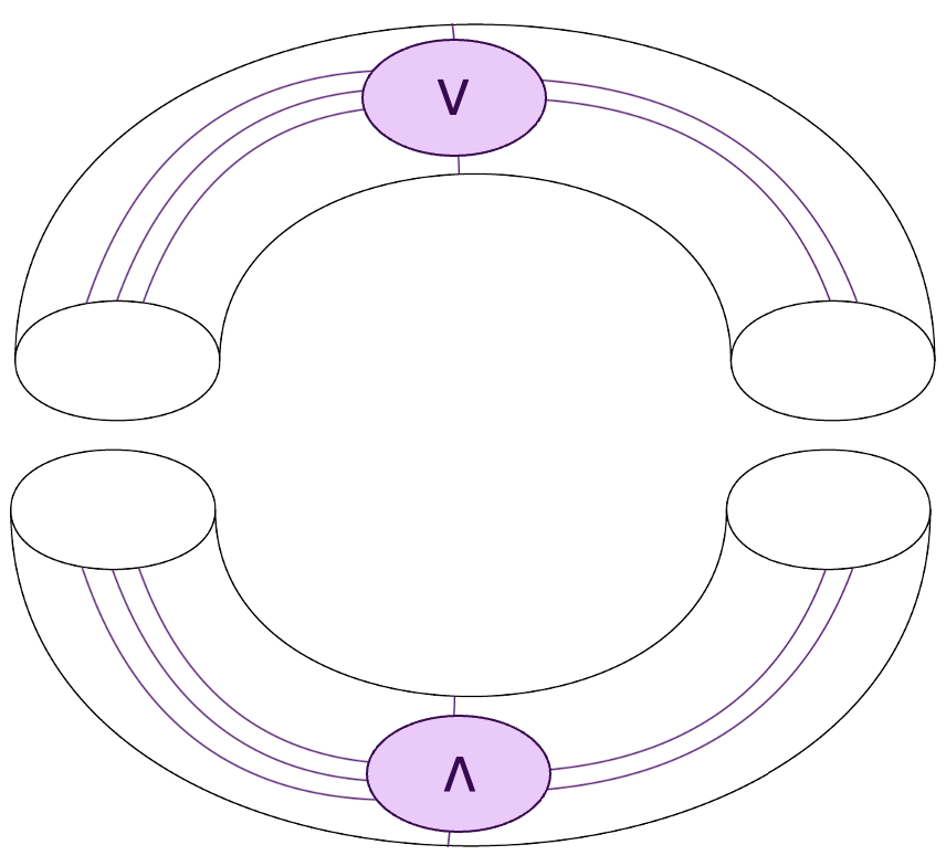
Figure 1. Gluing cylindrical cobordisms into an algebraic Lagrangian cobordism.

This can be seen as mirroring the fact that any rationally equivalent cycles are algebraically equivalent over an elliptic curve $E$ after a pullback by the double cover

$$E\longrightarrow\mathbb{P}^{1}.$$

In particular, there is a natural projection

$$\mathcal{C}ob(X)\stackrel{{\scriptstyle\pi}}{{\longrightarrow}}algCob(X),$$

and the cycle class maps from each of these groups coincide after factoring through $\pi$.

Example 3.6 (Abelian varieties).

Given a polarised tropical torus $B$, one can consider the oriented fibered cobordism group $\mathcal{C}ob_{fib}(X(B))$, that is the group generated by fibres $F_{b}$ for $b\in B$ in which relations come from cobordisms all of whose ends are fibres. It follows from flux considerations that there cannot exist an oriented cobordism between $F_{b}$ and $F_{b^{\prime}}$ for $b\neq b^{\prime}$. In fact, Sheridan–Smith prove in [SS21, Theorem 1.2] that $\mathcal{C}ob_{fib}(X(B))_{hom}$ is divisible (here they consider cylindrical cobordisms). This result mirrors an algebraic result about divisibility of (tropical) Chow groups, namely [Blo, Theorem 3.1], of which they prove a tropical version [SS21, Proposition 3.25]. On the other hand, the diagonal $\Delta\subset X(B)\times X(B)$ provides an obvious oriented algebraic Lagrangian cobordism between any two fibres $F_{b}$ and $F_{b^{\prime}}$, yielding $algCob(X(B))_{fib}\cong\mathbb{Z}$. This is a symplectic manifestation of the fact that any two points on an abelian variety $A$ lie on a curve, hence $\text{Griff}_{0}(A)\cong\mathbb{Z}$. Notice that while certain fluxes do obstruct the existence of algebraic Lagrangian cobordisms, this specific type of flux between fibres does not. This can be understood as a manifestation of Remark 5.11.

As noted in Remark 3.2, in the algebraic setting one can recover an algebraic equivalence of cycles over a curve from an algebraic equivalence of cycles over an abelian variety by considering the flat pullback to a curve between the two relevant points. We end this Section with a Lemma which is an analogous result for algebraic Lagrangian cobordisms:

Lemma 3.7.

Let $\Gamma:L\stackrel{{\scriptstyle X(B)_{p,q}}}{{\lx@xy@svg{\hbox{\raise 0.0pt\hbox{\kern 3.0pt\hbox{\ignorespaces\ignorespaces\ignorespaces\hbox{\vtop{\kern 0.0pt\offinterlineskip\halign{\entry@#!@&&\entry@@#!@\cr&\crcr}}}\ignorespaces{\hbox{\kern-3.0pt\raise 0.0pt\hbox{\hbox{\kern 0.0pt\raise 0.0pt\hbox{\hbox{\kern 3.0pt\raise 0.0pt\hbox{$\textstyle{{}\ignorespaces\ignorespaces\ignorespaces\ignorespaces}$}}}}}}}\ignorespaces\ignorespaces\ignorespaces{}\ignorespaces\ignorespaces{\hbox{\lx@xy@drawsquiggles@}}\ignorespaces{\hbox{\kern 27.0pt\raise 0.0pt\hbox{\hbox{\kern 0.0pt\raise 0.0pt\hbox{\lx@xy@tip{1}\lx@xy@tip{-1}}}}}}\ignorespaces\ignorespaces{\hbox{\lx@xy@drawsquiggles@}}\ignorespaces{\hbox{\lx@xy@drawsquiggles@}}{\hbox{\kern 27.0pt\raise 0.0pt\hbox{\hbox{\kern 0.0pt\raise 0.0pt\hbox{\hbox{\kern 3.0pt\raise 0.0pt\hbox{$\textstyle{}$}}}}}}}\ignorespaces}}}}\ignorespaces}}L^{\prime}$ be an algebraic Lagrangian cobordism. There exists a Lagrangian $\Gamma^{\prime}$ in $X\times X(B)$ such that $\pi_{B}(\Gamma^{\prime})\subset B$ is a tropical curve, and $\Gamma^{\prime}(F_{p})=L$, $\Gamma^{\prime}(F_{q})=L^{\prime}$.

Proof.

Because $B$ is polarised, it contains a tropical curve passing through any two given points. For our purposes, we want these curves to admit Lagrangian lifts. We use [SS21, Lemma 3.28], which states that, given a point $p$ on a polarised tropical torus $B$, there is an open dense subset $U_{p}$ of points in $B$ such that, for any point $q\in U_{p}$, $p$ and $q$ lie on edges of some trivalent tropical curve. Therefore, possibly after perturbing $\Gamma$ by a hamiltonian isotopy, one can take $p$ and $q$ to lie on edges of some trivalent tropical curve $C$ in $B$. The fact that trivalent tropical curves admit Lagrangian lifts follows independently from constructions of Matessi and Mikhalkin in [Mat21, Mik19], and is also proved in [SS21, Corollary 4.9] with additional properties of the lift (eg it is graded and locally exact). Let $L_{C}\subset X(B)$ denote such a lift. We now recall a construction of A. Subotic [Sub10] known as fibrewise sum in a Lagrangian torus fibration with a distinguished Lagrangian section, which in the case of a symplectic polarised torus $X(B)$ is the operation

$$\Sigma:\mathcal{F}uk(X(B))\times\mathcal{F}uk(X(B))\longrightarrow\mathcal{F}uk(X(B))$$

induced by the correspondence

$$\Sigma:=\{(x,p_{1},x,p_{2},x,p_{1}+p_{2}):x\in B,p_{1},p_{2}\in F_{x}\}\subset\overline{X\times X}\times X.$$

We now consider the correspondence $\varphi_{13425}(\Delta_{X}\times\Sigma)\subset\overline{X\times X(B)\times X(B)}\times X\times X(B)$, where $\Delta_{X}\subset X\times X$ is the diagonal, and

$$\varphi_{13425} :X\times X\times X(B)\times X(B)\times X(B)\longrightarrow X\times X(B)\times X(B)\times X\times X(B)$$

$$\hskip 56.9055pt(z_{1},z_{2},z_{3},z_{4},z_{5})\hskip 42.67912pt\mapsto\hskip 42.67912pt(z_{1},z_{3},z_{4},z_{2},z_{5})$$

is simply the map changing the order of the product components. This correspondence takes Lagrangians in $X\times X(B)\times X(B)$ to Lagrangians in $X\times X(B)$. From this we define $\Gamma^{\prime}$ as $\varphi_{13425}(\Delta_{X}\times\Sigma)(\Gamma\times L_{C})$. We check that $\Gamma^{\prime}(F_{p})=L$, and verifying $\Gamma^{\prime}(F_{q})=L^{\prime}$ is analogous. Notice that, by definition of $\Gamma^{\prime}$,

$$\Gamma^{\prime}(F_{p}) =\pi_{X}(\Gamma^{\prime}\pitchfork(X\times F_{p}))=\{x\in X:\exists f\in F_{p},(x,f)\in\Gamma^{\prime}))\}$$

$$=\{x\in X:\exists f,f_{1},f_{2}\in F_{p},(x,f_{1})\in\Gamma,f_{2}\in L_{C},f=f_{1}+f_{2}\}.$$

It remains to notice that because $\Gamma(F_{p})=L$, there exists $f_{1}\in F_{p}$ with $(x,f_{1})\in\Gamma$ if and only if $x\in L$. For $x\in L$, one can take any $f_{2}\in F_{p}\cap L_{C}$ to be the intersection of $F_{p}$ with the zero section in $X(B)$, then $f=f_{1}$ satisfies $(x,f)\in\Gamma^{\prime}$. ∎

3.2. Flux maps from $algCob(X)$

In this Section, we prove that some of the flux maps $\Theta_{\alpha}$ defined in 2 from $\mathcal{C}ob(X)$ (namely those with $\alpha$ of the form $\omega\wedge\beta$) factor through $\mathcal{C}ob(X)\stackrel{{\scriptstyle\pi}}{{\longrightarrow}}algCob(X)$.

Theorem 3.8.

For any closed form $\beta\in\Omega^{n-3}(X),$ there is a flux-type morphism

$$\tilde{\Theta}_{\beta}: \hskip 5.69054ptalgCob(X)_{hom}\longrightarrow\mathbb{R}/\left([\omega^{2}\wedge\beta]\cdot H_{n+1}(X)\right)$$

$$\hskip 25.60747ptL\hskip 48.36967pt\mapsto\hskip 34.1433pt\int_{\gamma_{0}}\omega^{2}\wedge\beta,$$

where $\gamma_{0}$ is an $(n+1)$-chain in $X$ with $\partial\gamma_{0}=L$.

Proof.

Assume there exists a Lagrangian correspondence $\Gamma\subset X\times X(B)$ between the finite sets of Lagrangians $(L_{1},\dots,L_{k})$ and $(L^{\prime}_{1},\dots,L^{\prime}_{k^{\prime}})$. It suffices to show that, if $\gamma_{0}$ is an $(n+1)$-chain in $X$ such that $\partial\gamma_{0}=L_{1}+\dots+L_{k}-L^{\prime}_{1}-\dots-L^{\prime}_{k^{\prime}}$, then

$$\int_{\gamma_{0}}\omega^{2}\wedge\beta\in[\omega^{2}\wedge\beta]\cdot H_{n+1}(X;\mathbb{Z}).$$

We proceed by constructing an $(n+1)$-cycle $C$ in $X\times X(B)$, and show on the one hand that the integral of $(\omega+\omega_{X(B)})^{2}\wedge\pi^{*}_{X}\beta$ on $C$ is the same as an integral over an $(n+1)$-chain $\gamma_{0}$ as above, and on the other hand that $C$ can be continuously deformed to an $(n+1)$-cycle in $X\times F_{p}$. The result will follow. Throughout the proof, we will assume all intersections we consider are transverse, which can always be achieved by a small hamiltonian perturbation of $\Gamma$.

We start by choosing a path

$$P:[0,1]\longrightarrow B$$

such that $P(0)=p$ and $P(1)=q$. Because $\pi_{B}(\Gamma)=B$, for all $t\in[0,1]$, $\pi^{-1}_{B}(P(t))\cap\Gamma$ is non-empty. We write

$$C_{1}:=\Gamma\cap(\pi^{-1}_{B}(P([0,1]))).$$

Recall that the flat connection determined by the affine structure on $B$ defines a canonical parallel transport map

$$\varphi_{\gamma}:\hskip 2.84526pt [0,1]\times\{q\}\times F_{q}\longrightarrow\pi_{B}^{-1}(\gamma([0,1]))\subset X(B)$$

$$\hskip 25.60747pt(t,y)\hskip 34.1433pt\mapsto\hskip 2.84526pt(\gamma(t),\tilde{\varphi}(t,y))$$

for any path $\gamma:[0,1]\rightarrow B$ with $\gamma(0)=q$, where $\tilde{\varphi}(t,y)\in F_{\gamma(t)}$ is the parallel transport along $\gamma([0,t])$ of $y\in F_{q}$. From this, we define $C_{2}$ as the image of the embedding

$$[0,1]\times(\Gamma\cap(X\times F_{q}))\longrightarrow X\times X(B)$$

$$\hskip 39.83385pt(t,x,q,y)\hskip 28.45274pt\mapsto\hskip 2.84526pt(x,\varphi_{\overline{P}}(t,y)),$$

where $\overline{P}$ denotes the path $P$ with the orientation reversed, and $x\in X$ while $y\in F_{q}$. Notice that $C_{1}\cup C_{2}$ is an $(n+1)$-chain in $X\times X(B)$ with boundary in $X\times F_{p}$, and more precisely $\pi_{X}(\partial(C_{1}\cup C_{2}))=L_{1}+\dots+L_{k}-L^{\prime}_{1}-\dots-L^{\prime}_{k^{\prime}}\subset X$. The fact that the boundary component in $X\times F_{q}$ is empty simply follows from the fact that the boundaries of $\partial C_{1}$ and $\partial C_{2}$ cancel out by construction of $C_{2}$.

Our next step is to construct an $(n+1)$-chain $C_{3}$ inside $X\times F_{p}$ with $\partial C_{3}=\partial(C_{1}\cup C_{2})\subset X\times F_{p}$. Here we use parallel transport again from the fibres $F_{P(t)}$ to $F_{p}$, this time sending $\Gamma\cap(X\times F_{P(t)})$ to $X\times F_{p}$. More explicitly, we take $C_{3}$ to be the image of the map

$$C_{1}\hskip 17.07164pt \longrightarrow\hskip 11.38109ptX\times F_{p}$$

$$(x,P(t),f) \hskip 2.84526pt\mapsto(x,p=P(0),\tilde{\varphi}_{\tilde{P}_{t}}(1,f)),$$

where $x\in X$, $f\in F_{P(t)}$, and $\tilde{P}_{t}:[0,1]\rightarrow B$ is defined by $\tilde{P}_{t}(s):=P(t(1-s))$. From this construction it follows that $C_{3}$ is $(n+1)$-dimensional except in the trivial case where $C_{1}=C_{2}$ as a set, in which case it is $n$-dimensional, and in particular this would imply $L_{1}+\dots+L_{k}=L^{\prime}_{1}+\dots+L^{\prime}_{k^{\prime}}$. Putting all this together, we have constructed an $(n+1)$-cycle

$$C:=C_{3}-C_{1}-C_{2}$$

inside $X\times X(B)$. We now compute the integral

(3.1) $$\int_{C}\left(\pi_{X}^{*}\omega+\pi_{X(B)}^{*}\omega_{X(B)}\right)^{2}\wedge\pi_{X}^{*}\beta$$

in two different ways. The first way involves noticing that the only contributions to this integral come from integrating over $C_{3}$. The fact that the contributions from $C_{1}$ vanish follows from the fact that

$$\left(\pi_{X}^{*}\omega+\pi_{X(B)}^{*}\omega_{X(B)}\right)|_{C_{1}}=0$$

because $TC_{1}\subset T\Gamma$ and $\Gamma$ is Lagrangian. Although the same doesn’t necessarily hold for $C_{2}$, it is true that

$$\left(\pi_{X}^{*}\omega+\pi_{X(B)}^{*}\omega_{X(B)}\right)^{2}|_{C_{2}}=0.$$

To see this, one can decompose the tangent space to $C_{2}\subset X\times X(B)$ at any point $(x,P(t),f_{P(t)})\in C_{2}$. The component along $X$ lives in an isotropic subspace of $T_{x}X$, because $C_{2}$ is parallel transport of $\Gamma\cap(X\times F_{q})$. By considering the trivialisation

$$t_{b}:X(B)\longrightarrow B\times F_{b}$$

given by parallel transport, one sees that the component along $T_{P(t)}B$ is one-dimensional, therefore $\omega_{X(B)}^{2}$ necessarily vanishes along the $X(B)$ direction.

We have now reduced the integral 3.1 to

$$\int_{C_{3}}\left(\pi_{X}^{*}\omega+\pi_{X(B)}^{*}\omega_{X(B)}\right)^{2}\wedge\pi_{X}^{*}\beta=\int_{C_{3}}\pi_{X}^{*}(\omega^{2}\wedge\beta)=\int_{(\pi_{X})_{*}C_{3}}\omega^{2}\wedge\beta.$$

Here the first equality follows from the fact that $C_{3}$ is contained in $X\times F_{p}$ and $F_{p}$ is Lagrangian in $X(B)$. Notice that wa have exhibited an $(n+1)$-chain in $X$, namely $(\pi_{X})_{*}C_{3}$, whose boundary is $L_{1}+\dots+L_{k}-L^{\prime}_{1}-\dots-L^{\prime}_{k^{\prime}}$, and over which $\omega^{2}\wedge\beta$ integrated to something which lies in

$$[\left(\pi_{X}^{*}\omega+\pi_{X(B)}^{*}\omega_{X(B)}\right)^{2}\wedge\pi_{X}^{*}\beta]\cdot H_{n+1}(X\times X(B);\mathbb{Z}).$$

The aim of the second computation of 3.1 is to show that the integral over $C$ can actually be reduced to an integral of $\omega^{2}\wedge\beta$ over an $(n+1)$-cycle in $X$. That is, 3.1 actually lies in

$$[\omega^{2}\wedge\beta]\cdot H_{n+1}(X;\mathbb{Z})\subset[\left(\pi_{X}^{*}\omega+\pi_{X(B)}^{*}\omega_{X(B)}\right)^{2}\wedge\pi_{X}^{*}\beta]\cdot H_{n+1}(X\times X(B);\mathbb{Z}).$$

This follows from the trivial fact that the composition of paths $\overline{P}\star P$ is contractible. Denote by

$$r:[0,1]^{2}\rightarrow B$$

a homotopy to $\{p\}$, that is $r(0,s)=p=r(1,s)$, $r(s,0)=\overline{P}\star P(s)$ and $r(s,1)=p$. This induces a strong deformation retraction

$$R(1):\pi_{B}^{-1}(P([0,1]))\longrightarrow X\times F_{p},$$

again obtain by parallel transport through the following family of maps parametrised by $s\in[0,1]$:

$$R(s): \hskip 2.84526pt\pi_{B}^{-1}(P([0,1]))\longrightarrow\pi_{B}^{-1}(r([0,1],s))$$

$$\hskip 8.53581pt(x,P(t),f)\hskip 8.53581pt\mapsto(x,r(t,s),\varphi_{r(t,\cdot)}(f)).$$

Noticing that $C\subset\pi_{B}^{-1}(P([0,1]))$, this allows us to compute 3.1:

$$\int_{C}\left(\pi_{X}^{*}\omega+\pi_{X(B)}^{*}\omega_{X(B)}\right)^{2}\wedge\pi_{X}^{*}\beta =\int_{R(1)_{*}C}\left(\pi_{X}^{*}\omega+\pi_{X(B)}^{*}\omega_{X(B)}\right)^{2}\wedge\pi_{X}^{*}\beta$$

$$=\int_{R(1)_{*}C}\pi_{X}^{*}(\omega^{2}\wedge\beta)$$

$$=\int_{(\pi_{X}\circ R(1))_{*}C}\omega^{2}\wedge\beta.$$

It remains to observe that $(\pi_{X}\circ R(1))_{*}C$ is an $(n+1)$-cycle in $X$, therefore we have shown that

$$\int_{C}\left(\pi_{X}^{*}\omega+\pi_{X(B)}^{*}\omega_{X(B)}\right)^{2}\wedge\pi_{X}^{*}\beta=\int_{(\pi_{X})_{*}C_{3}}\omega^{2}\wedge\beta$$

lies in the periods of $\omega^{2}\wedge\beta$, from which we conclude the proof. ∎

The following is immediate by comparing the definition of the flux maps from $\mathcal{C}ob^{or}(X)$ and $algCob^{or}(X)$.

Corollary 3.9.

For $\alpha=\omega\wedge\beta$, the flux morphisms $\Theta_{\alpha}$ and $\tilde{\Theta}_{\beta}$ defined from $\mathcal{C}ob^{or}(X)$ and $algCob^{or}(X)$ factor through the projection map as follows

3.3. A Lefschetz Jacobian

In this Section, we reformulate the flux maps constructed in 2.1 and 3.2 as “symplectic Abel-Jacobi maps” to a Lefschetz Jacobian. These can be thought of as a symplectic analogue of intermediate Jacobians. We work under the assumption that $X$ is a Lefschetz manifold, that is the maps

$$\cup[\omega]^{k}:H^{n-k}(X;\mathbb{R})\longrightarrow H^{n+k}(X;\mathbb{R})$$

are isomorphisms for all $0\leq k\leq n$.

Letting $\mathcal{L}^{or}$ be a set of suitable oriented Lagrangians in $X$, define $\mathbb{L}^{or}:=\oplus_{L\in\mathcal{L}}\mathbb{Z}\cdot L$. This comes with an obvious cycle class map

$$cyc:\mathbb{L}^{or}\longrightarrow H_{n}(X;\mathbb{Z}),$$

whose kernel we denote $\mathbb{L}^{or}_{hom}$.

There is a generalised flux map map

$$\Theta:\hskip 17.07164pt\mathbb{L}^{or}_{hom}\hskip 17.07164pt \longrightarrow LJ(X):=H^{n+1}(X;\mathbb{R})^{\vee}/H_{n+1}(X;\mathbb{Z})$$

$$L\hskip 25.60747pt \mapsto\hskip 39.83385pt\left([\eta]\mapsto\int_{\gamma}\eta\right),$$

where $\partial\gamma=L$. This is independent of the choice of such $\gamma$ because we view $H_{n+1}(X;\mathbb{Z})$ as a lattice inside $H^{n+1}(X;\mathbb{R})^{\vee}$ through the usual integration map over $(n+1)$-cycles. To see that $\Theta$ is well-defined at the level of cohomology, notice that an exact $(n+1)$-form $d\nu$ must be of the form $\omega\wedge d\mu=d(\omega\wedge\mu)$ for some $(n-2)$-form $\mu$. Therefore

$$\int_{\gamma}d\eta=\int_{L}\omega\wedge\mu=0.$$

Given an algebraic Lagrangian cobordism $\Gamma\subset X\times X(B)$, and given a choice of basepoint $b_{0}\in B$, one can consider the map

$$\varphi_{\Gamma}:B \longrightarrow LJ(X)$$

$$b \mapsto\Theta(\Gamma(F_{b}-F_{b_{0}})).$$

A special instance of this is

$$\varphi_{\Delta}:B\longrightarrow LJ(X(B))$$

induced by the diagonal $\Delta\subset X(B)\times X(B)$, which provides an algebraic Lagrangian cobordism between any pair of fibres $F_{p}$, $F_{q}$ in $X(B)$. Below we show that the real torus $LJ(X(B))$ can be endowed with a tropical structure making $\varphi_{\Delta}$ into a tropical embedding.

It follows from Theorem 3.5 and by the fact that $H^{n+1}(X;\mathbb{R})\cong[\omega]\cup H^{n-1}(X;\mathbb{R})$ that nullcobordant elements in $\mathbb{L}^{or}_{hom}$ lie in the kernel of $\Theta$. In other words, $\varphi_{\Gamma}$ factors as

Similarly, Theorem 3.2 implies that algebraically nullbordant elements in $\mathbb{L}^{or}_{hom}$ are mapped to the subset

(3.2) $$\left(H^{n+1}(X;\mathbb{R})/([\omega]^{2}\cup H^{n-3}(X;\mathbb{R}))\right)^{\vee}\subset\left(H^{n+1}(X;\mathbb{R})\right)^{\vee}.$$

We now describe a tropical structure for $LJ(X)$ by choosing a lattice in $(H^{n+1}(X;\mathbb{R}))^{\vee}$ of those maps $H^{n+1}(X;\mathbb{R})\longrightarrow\mathbb{R}$ which evaluate to integers on a certain sublattice $H^{n+1}(X;\mathbb{R})_{\mathbb{Z}}$ of $H^{n+1}(X;\mathbb{R})$. To define $H^{n+1}(X;\mathbb{R})_{\mathbb{Z}}$, we invoke the Lefschetz decomposition

$$H^{n+1}(X;\mathbb{R})\cong\bigoplus_{i}[\omega]^{i}\cup\ker([\omega]^{2i}:H^{n-2i+1}(X;\mathbb{R})\longrightarrow H^{n+2i+1}(X;\mathbb{R})).$$

From this we set

(3.3) $$H^{n+1}(X;\mathbb{R})_{\mathbb{Z}}:=\bigoplus_{i}[\omega]^{i}\cup\ker([\omega]^{2i}:H^{n-2i+1}(X;\mathbb{Z})\longrightarrow H^{n+2i+1}(X;\mathbb{R})).$$

Unless otherwise stated, from now on when referring to $LJ(X)$ as a tropical object we endow it with the aforementioned tropical structure.

Proposition 3.10.

A polarised tropical torus $B$ embeds tropically into the Lefschetz Jacobian $LJ(X(B))$.

Proof.

Let $\Delta\subset X(B)\times X(B)$ be the diagonal, which as we have seen, provides an algebraic Lagrangian cobordism between any pair of fibres $F_{p}$, $F_{q}$ in $X(B)$. We will show that the map

$$\varphi_{\Delta}:B\longrightarrow LJ(X(B))$$

is a embedding, where we have chosen a basepoint $b_{0}\in B$. For any $b_{0}\neq b\in B$, we consider a line segment $\{b_{0}+tv\}_{t\in[0,1]}$ between $b_{0}$ and $b$, where $v\in TB\cong\mathbb{R}^{n}$. This traces out a Lagrangian isotopy $\{F_{b_{0}+tv}\}_{t\in[0,1]}$ between $F_{b_{0}}$ and $F_{b}$, and the image $\varphi_{\Delta}(b)\in LJ(X(B))$ can be seen as integration of $(n+1)$-forms along this isotopy, modulo integration over $(n+1)$-cycles.

We start by understanding the differential

$$(\varphi_{\Delta})_{*}:TB\longrightarrow TLJ(X(B)),$$

using the observation above. Recall that up to a global coordinate transformation, $B\cong B(M):=\mathbb{R}^{n}/M\cdot\mathbb{Z}^{n}$ for some $M\in GL(n;\mathbb{R})$, where $\mathbb{R}^{n}$ is considered with the tropical structure given by the integer lattice $\mathbb{Z}^{n}\subset\mathbb{R}^{n}$. Given $v\in TB\cong\mathbb{R}^{n}$, there is a corresponding element $[v]\in H_{1}(B;\mathbb{R})$ obtained by identifying $H_{1}(B;\mathbb{R})\cong(M\cdot\mathbb{Z}^{n})\otimes\mathbb{R}\cong TB$. Fixing a point $b\in B$, a fundamental class $[F_{b}]\in H_{n}(F_{b};\mathbb{Z})$, and using the Künneth isomorphism

$$\psi:\bigoplus_{k=1}^{n}H^{k}(B;\mathbb{R})\otimes H^{n+1-k}(F_{b};\mathbb{R})\stackrel{{\scriptstyle\cong}}{{\longrightarrow}}H^{n+1}(X(B);\mathbb{R}),$$

the differential is simply

$$v\mapsto\psi([v]\otimes[F_{b}]),$$

which is injective. Injectivity of $\varphi_{\Delta}$ follows from the fact that it acts linearly with respect to scaling the vector $v$, from which we can deduce that $\varphi_{\Delta}(b)\neq 0\mod H_{n+1}(X(B);\mathbb{Z})$ unless $v\in H_{1}(B;\mathbb{Z})$.

The fact that the tropical structure defined by 3.3 makes $\varphi_{\Delta}$ into a tropical map follows from the observation that if $v\in T_{\mathbb{Z}}B$, then $[v]\otimes[F_{b}]\in M^{-1}\cdot H_{1}(B;\mathbb{Z})\otimes H_{n}(F_{b};\mathbb{Z}).$ This corresponds to maps $H^{n+1}(X(B);\mathbb{R})\longrightarrow\mathbb{R}$ which evaluate to integers on the lattice

$$\psi\left(M^{t}\cdot H^{1}(B;\mathbb{Z})\otimes H^{n}(F_{b};\mathbb{Z})\right)\subset H^{n+1}(X(B);\mathbb{R}).$$

Now notice that

$$[\omega]\in\psi\left(M^{t}\cdot H^{1}(B;\mathbb{Z})\otimes H^{1}(F_{b};\mathbb{Z})\right)$$

as it evaluates to integers on homology classes corresponding to

$$M^{-1}\cdot H_{1}(B;\mathbb{Z})\otimes H_{1}(F_{b};\mathbb{Z}).$$

In particular,

$$\psi\left(M^{t}\cdot H^{1}(B;\mathbb{Z})\otimes H^{n}(F_{b};\mathbb{Z})\right)\subset[\omega]\cup\ker([\omega]^{2}:H^{n-1}(X(B);\mathbb{Z})\longrightarrow H^{n+1}(X(B);\mathbb{R})),$$

from which we conclude. ∎

Remark 3.11.

It follows from 3.2 that the proof of tropicality of a map $\varphi_{\Gamma}:B\longrightarrow LJ(X)$ induced by an algebraic Lagrangian cobordism $\Gamma\subset X(B)\times X$ only depends on the choice of tropical structure in first component of the Lefschetz decomposition, that is in

$$[\omega]\cup\ker([\omega]^{2}:H^{n-1}(X;\mathbb{R})\longrightarrow H^{n+3}(X;\mathbb{R})).$$

Additionally, in this instance where $\Gamma=\Delta\subset X(B)\times X(B)$, the only component relevant to the tropical structure is

$$[\omega]\cup\psi\left(H^{0}(B;\mathbb{R})\otimes H^{n-1}(F_{b};\mathbb{R}))\right)\subset[\omega]\cup\ker([\omega]^{2}:H^{n-1}(X;\mathbb{R})\longrightarrow H^{n+3}(X;\mathbb{R})).$$

This is related to the fact that all of the Lagrangians considered here are fibres; one expects that the terms contained in

$$[\omega]\cup\psi\left(\bigoplus_{i\geq 1}H^{i}(B;\mathbb{R})\otimes H^{n-i-1}(F_{b};\mathbb{R}))\right)$$

would become relevant if one were to consider eg Lagrangians lifts in $X(B)$ of tropical $k$-cycles in $B$ with $k\geq 1$.

4. Tropical background

4.1. Tropical tori

We will be concerned with tropical tori, which are a particularly simple example of tropical manifold.

Definition 4.1.

Let $B$ be a smooth manifold. A tropical affine structure on $B$ is a set of coordinate charts $\{(U_{i},\varphi_{i})\}$ on $B$ such that for all $i,j$, the transition maps $\varphi_{i}\circ\varphi_{j}^{-1}$ lie in $\mathbb{R}^{n}\rtimes GL(n;\mathbb{Z})$. That is, they are of the form $x\mapsto Ax+b$ with $A\in GL(n;\mathbb{Z})$ and $b\in\mathbb{R}^{n}$. We call $B$ endowed with such a structure a tropical manifold.

Remark 4.2.

The base $B$ of a complete integrable system $X\rightarrow B$ carries a canonical tropical affine structure given by the action-angle coordinates [Eva22, Section 2.3].

From such a structure one can define a subsheaf $\textit{Aff}_{B}\subset C^{\infty}(B)$ of the sheaf of smooth functions, consisting of those functions which in any coordinate chart $(U_{i},\varphi_{i})$ are affine-linear with integer slope. Their differentials form a local system of rank $n$ lattices $T^{*}_{\mathbb{Z}}B$ inside $T^{*}B$. Equivalently, there is a short exact sequence of sheaves

$$0\longrightarrow\underline{\mathbb{R}}\longrightarrow\textit{Aff}_{B}\longrightarrow T_{\mathbb{Z}}^{*}B\longrightarrow 0.$$

Elements of the group of global sections $H^{0}(T_{\mathbb{Z}}^{*}B)$ are called tropical $1$-forms. Furthermore, there is a dual lattice $T_{\mathbb{Z}}B\subset TB$ of those vectors on which $T_{\mathbb{Z}}^{*}B$ evaluate to integers, and elements of $H^{0}(T_{\mathbb{Z}}B)$ are called integral vectors.

In the case where $B:=\mathbb{R}^{n}/\Gamma$ is a torus, the linear part of the monodromy on the sheaf of affine functions vanishes, and the local systems $T^{(*)}_{\mathbb{Z}}B$ are trivial. Therefore a tropical torus $B$ is simply the data of two rank $n$ lattices $\Gamma_{1}$ and $\Gamma_{2}$ in $\mathbb{R}^{n}$, such that $B=\mathbb{R}^{n}/\Gamma_{1}$ and the tropical structure on $B$ is given by $T_{\mathbb{Z}}B=\Gamma_{2}\subset\mathbb{R}^{n}$. Up to a global coordinate transformation, one can take $\Gamma_{2}$ to be the standard lattice $\mathbb{Z}^{n}\subset\mathbb{R}^{n}$, then a tropical torus is determined by a matrix $M$ in $GL(n;\mathbb{R})$ such that $B=B(M):=\mathbb{R}^{n}/M\cdot\mathbb{Z}^{n}$ (note that left or right multiplication of $M$ by elements of $GL(n;\mathbb{Z})$ yield isomorphic tropical tori, see eg [SS21, Lemma 2.4]).

A polarisation on a tropical torus $B$ is a class in $H^{1}(T^{*}_{\mathbb{Z}}B)$ in the image of the tropical Chern class map

$$H^{1}(\textit{Aff}_{B})\longrightarrow H^{1}(T_{\mathbb{Z}}^{*}B).$$

From the isomorphism $H^{1}(T^{*}_{\mathbb{Z}}B)\cong\Gamma_{1}^{*}\otimes H^{0}(T^{*}_{\mathbb{Z}}B)\cong\hom(H_{1}(B;\mathbb{Z}),H^{0}(T_{\mathbb{Z}}^{*}B))$ this can be shown [MZ08, Section 5.1] to be equivalent to a map

$$c:H_{1}(B;\mathbb{Z})\longrightarrow H^{0}(T_{\mathbb{Z}}^{*}B)$$

such that the induced pairing on $H_{1}(B;\mathbb{Z})$ given by $\int_{\gamma_{i}}c(\gamma_{j})$ is positive-definite and symmetric. A polarisation is principal if this map is an isomorphism.

4.2. Tropical curves, their Jacobian and their Ceresa cycle

We summarize the tropical version of the classical construction of the Jacobian of a curve and its Abel-Jacobi embedding, and give the definition of the tropical Ceresa cycle.

Definition 4.3.

A tropical curve consists of a finite connected graph $G$ together with a positive function $l:E(G)\longrightarrow\mathbb{R}_{\geq 0}$ on its edge set $E(G)$. Given $e\in E(G)$, $l(e)$ is called the length of $e$.

Remark 4.4.

As such, $C$ is not quite a tropical manifold of dimension $1$ as in Definition 4.1, but falls into the more general notion of tropical space [MR, Definition 7.1.8]. The two can be shown to be equivalent [MR, Section 8.1] if one additionally requires $C$ to be smooth, regular at infinity, and of finite type [MR, Definition 7.4.1]. For our purposes these assumptions are not restrictive, and we extend our constructions on tropical manifolds to tropical curves, where the tropical structure on the latter can be obtained by embedding edges of $C$ in $\mathbb{R}$ via metric-preserving charts (for more details, consult eg [MZ08, Proposition 3.6]).

If the underlying graph of $C$ has genus $g$, then $H^{0}(T_{\mathbb{Z}}^{*}C)$ is a free abelian group of rank $g$, in particular $H^{0}(T_{\mathbb{R}}^{*}C):=H^{0}(T_{\mathbb{Z}}^{*}C)\otimes\mathbb{R}\cong\mathbb{R}^{g}$. We define the tropical Jacobian of $C$ as the torus

$$J(C):=H^{0}(T_{\mathbb{R}}^{*}C)^{*}/H_{1}(C;\mathbb{Z}),$$

where $H_{1}(C;\mathbb{Z})$ is idetified with a lattice inside $H^{0}(T_{\mathbb{R}}^{*}C)^{*}$ by setting $\gamma(\alpha):=\int_{\gamma}\alpha$ for any $\alpha\in H^{0}(T_{\mathbb{R}}^{*}C)$.

Given a choice of basepoint $p\in C$, the tropical Abel-Jacobi map

$$AJ_{p}:\hskip 5.69054pt C\longrightarrow J(C)$$

$$q\mapsto\left(\alpha\in\Omega^{1}(C)\mapsto\int_{\gamma:p\rightarrow q}\alpha\right)$$

embeds $C$ into $J(C)$, where $\gamma:p\rightarrow q$ is any path in $C$ between $p$ and $q$.

The Jacobian torus $J(C)$ carries both a canonical tropical structure given by the lattice $\Gamma_{2}\subset H^{0}(T_{\mathbb{R}}^{*}C)^{*}$ of those maps which evaluate to integers on global sections of $T_{\mathbb{Z}}C$, and a canonical principal polarisation which we describe following [MZ08, Section 6.1]. The bilinear form on the space of paths in $C$ defined by

$$Q(E,E):=l(E)$$

on any edge $E$ of $C$, then extended bilinearly, induces a symmetric, positive-definite bilinear form on $H_{1}(C;\mathbb{Z})\cong H_{1}(J(C);\mathbb{Z})$, therefore a polarisation

$$c(C):H_{1}(J(C);\mathbb{Z})\longrightarrow H^{0}(T^{*}_{\mathbb{Z}}J(C))$$

by $\int_{\gamma_{i}}c(\gamma_{j}):=Q(\gamma_{i},\gamma_{j})$.

One can show [MZ08, Lemma 6.3] that the tropical structure on $J(C)$ makes $AJ_{p}$ into a tropical map, that is $(AJ_{p})^{*}\textit{Aff}_{J(C)}=\textit{Aff}_{C}$. In the language of tropical Chow groups [AR10], this implies that $AJ_{p}(C)$ is a tropical $1$-cycle inside $J(C)$ which we write $C\in CH_{1}(J(C))$.

Furthermore, $J(C)$ inherits a group structure from the one on $H^{0}(T_{\mathbb{R}}^{*}C)^{*}$, hence carries a natural involution

$$(-1):J(C)\longrightarrow J(C)$$

given by inverse for the group law. The Ceresa cycle of $C$ is

$$AJ_{p}(C)-(-1)_{*}(AJ_{p}(C))\in CH_{1}(J(C)).$$

We will often abuse notation and write $C$ instead of $AJ_{p}(C)$, $C^{-}$ instead of $(-1)_{*}(AJ_{p}(C))$, and the Ceresa cycle simply as $C-C^{-}$.

Whenever $C$ is a hyperelliptic curve, $C-C^{-}$ is algebraically trivial. In fact, taking the basepoint $p$ to be a Weierstrass point, one finds that $AJ_{p}(C)=(-1)_{*}(AJ_{p}(C))$. However, as soon as $g(C)\geq 3$, the Ceresa cycle (whether in its classical or tropical version) has been the object of extensive study for being an example of a cycle which is homologically, but not algebraically, trivial. The following result is originally due to Ceresa in the classical setting [Cer83], but its tropical version was proved by Zharkov:

Theorem 4.5.

[Zha13, Theorem 3] Let $C$ be a generic genus $3$ tropical curve of type $K4$. Then $C$ is not algebraically equivalent to $C^{-}$ in its Jacobian $J(C)$.

A tropical curve of type $K4$ is a tropical curve such as the one represented in Figure 2. While there are five generic types of genus $3$ tropical curves (see Figure 7), our results do not apply to the four others; it is the aim of Section 8.1 to address this.

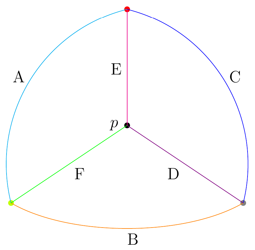
Figure 2. A tropical curve of type $K4$.

Remark 4.6.

Theorem 4.5 is only non-trivial because the Ceresa cycle is nullhomologous. In the classical case, this follows from the fact that $(-1)$ acts trivially on $H_{j}(J(C);\mathbb{Z})$ for $j$ even. Tropically, the tautological tropical cycles (see 5.1) associated to $C$ and $C^{-}$ in $J(C)$ are also homologically equivalent; in fact Zharkov exhibits a $\gamma_{0}\in C_{2}(J(C);T_{\mathbb{Z}}J(C))$ such that $\partial\gamma_{0}=\overline{C}-\overline{C^{-}},$ where $\overline{C}$ is the tautological tropical cycle defined in Section 5.1.

Remark 4.7.

The stronger statement that $C-C^{-}$ has infinite order in $CH_{1}(J(C))$ modulo algebraic equivalence follows from Zharkov’s proof, and is proved by Ceresa in the classical setting [Cer83]. We address this again in 7.4.

4.3. An important example: the genus $3$ curve of type $K4$

Here we exhibit some of the features of tropical curves and their Jacobians described above in the example which will be of primary interest to us; namely the genus $3$ curve of type $K4$. Figure 3 shows bases $\{\gamma_{1},\gamma_{2},\gamma_{3}\}$ of $H_{1}(C;\mathbb{Z})=\Gamma_{1}$ as well as $\{e_{1},e_{2},e_{3}\}$ of $\Gamma_{2}$. The coordinates of the former basis vectors in terms of the latter are

$$\gamma_{1}=(a+f+e,-f,-e) \gamma_{2}=(-f,b+d+f,-d) \gamma_{3}=(-e,-d,c+d+e),$$

where lowercase letters denote the length of the edge labelled by the corresponding uppercase letter.

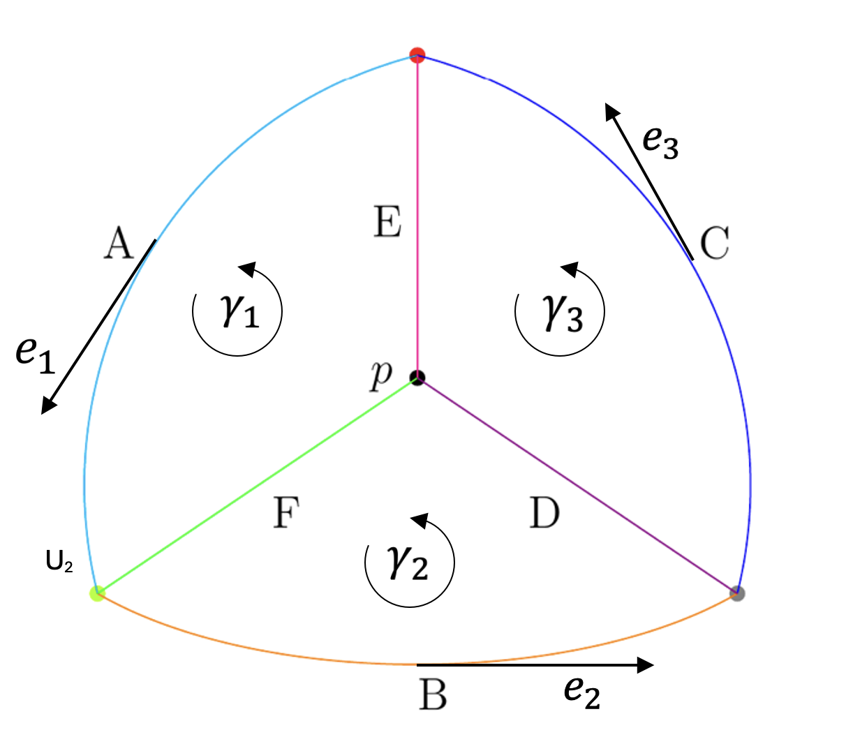
Figure 3. Bases for $\Gamma_{1}$ and $\Gamma_{2}$ represented in $C$.

In the colour-coded figure 4, we represent the image of $C$ in its Jacobian by the Abel-Jacobi map $AJ_{p}$, with the arbitrary choices of edge lengths

$$a=2 b=1 c=4 d=3 e=5 f=4.$$

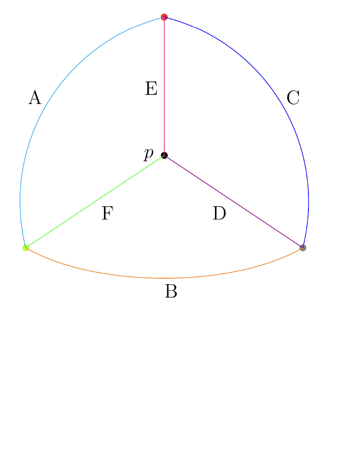
((a))

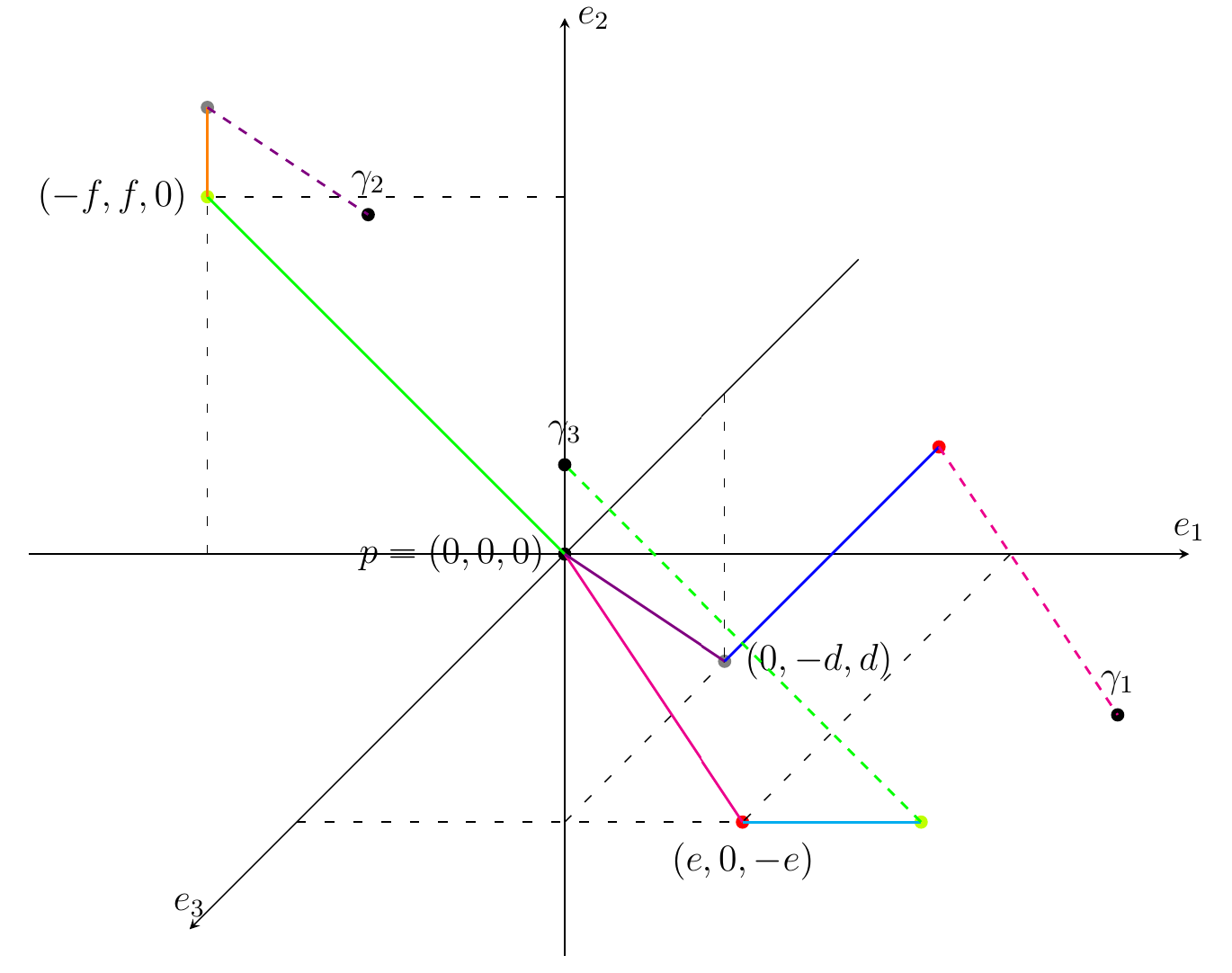
((b))

Figure 4. A non-hyperelliptic genus $3$ tropical curve in $(\text{A})$, and a representation of its embedding in $J(C)$ in $(\text{B})$; edges and vertices of the same color are identified.

4.4. Tropical (co)homology

Tropical (co)homology was originally introduced in [Ite+19], with the idea of encoding information about the (co)homology of an algebraic variety in the tropical (co)homology of its tropicalization. This is done by enriching singular (co)chains with coefficients in the exterior powers of the integral lattices $T_{\mathbb{Z}}^{(*)}B$ of a tropical manifold $B$, as a way of recording data from the tropical structure. In the case where $B$ is a tropical torus, we have seen that the local systems of lattices $T_{\mathbb{Z}}^{(*)}B$ are constant, therefore these are just global coefficients.

For any $k\geq 0$, we consider the chain complexes $C_{j}(B;\Lambda^{k}T_{\mathbb{Z}}B),$ whose objects are $j$-simplices $\sigma:\Delta\rightarrow B$ with coefficients in $\Lambda^{k}T_{\mathbb{Z}}B\cong\Lambda^{k}\Gamma_{2}$. The boundary map is given by restricting coefficients to the usual boundary map on singular $j$-chains. The resulting homology groups are denoted by $H_{j}(B;\Lambda^{k}T_{\mathbb{Z}}B)$. Similarly, we define the cohomology groups $H^{j}(B;\Lambda^{k}T^{*}_{\mathbb{Z}}B)$ for any $k$, by taking the cohomology of the dual complex $C^{j}(B;\Lambda^{k}T_{\mathbb{Z}}^{*}B)$. The universal coefficient theorem yields canonical isomorphisms:

$$H_{j}(B;\Lambda^{k}T_{\mathbb{Z}}B)\cong\Lambda^{j}\Gamma_{1}\otimes\Lambda^{k}\Gamma_{2}$$

$$H^{j}(B;\Lambda^{k}T_{\mathbb{Z}}^{*}B)\cong\Lambda^{j}\Gamma^{*}_{1}\otimes\Lambda^{k}\Gamma^{*}_{2}.$$

5. Tropical flux

A gap can be bridged between the symplectic flux obstructions described in Section 2, and ideas from Zharkov’s paper [Zha13] on the tropical Ceresa cycle, which proves Theorem 4.5. The key tool in its proof is the determinantal form $\Omega_{0}$, which is a $T^{*}_{\mathbb{Z}}J(C)$-valued $2$-form whose purpose is to detect obstructions to two $1$-cycles being algebraically equivalent.

We extend the idea of this proof by generalising determinantal forms to higher dimensions in any tropical torus $B$, and introducing the notion of tropical flux as morphisms

$$\Theta_{k}:\text{Griff}_{k}(B)\longrightarrow\mathbb{R}/\mathcal{P}_{k}.$$

Here $\text{Griff}_{k}(B)$ if the $k$-th Griffiths group of $B$ of homologically trivial $k$-cycles modulo algebraic equivalence, and $\mathcal{P}_{k}$ is the period lattice of a corresponding determinantal form.

In Section 6 we will show that, for a torus $B$, these tropical fluxes between tropical cycles translate to symplectic fluxes between their Lagrangian lifts in the symplectic manifold $X(B):=T^{*}B/T^{*}_{\mathbb{Z}}B$ in the sense of Section 2.

5.1. Tropical chains from algebraic equivalences

This section does not contain any original ideas, but extends constructions of Zharkov [Zha13, Section 3.1] from the case of $1$-cycles to that of arbitrary $k$-cycles. We borrow some of the notation and terminology for the sake of consistency. Note that here $B$ could be any tropical manifold, not just for a tropical torus.

Our first aim is to translate algebraic equivalence of cycles into the language of tropical (co)chains, in order to obtain tropical (co)homological obstructions to two cycles being algebraic equivalent. This requires two steps. The first is to associate to an algebraic cycle a tautological tropical cycle. The second is, given an algebraic equivalence between two cycles, to construct a tropical chain realising the tropical homological equivalence between the corresponding tautological tropical cycles.

Definition 5.1.

An algebraic $k$-cycle in $B$ is a weighted balanced $k$-dimensional polyhedral complex with $\Gamma_{2}$-rational slopes.

Two such cycles $Z_{1}$ and $Z_{2}$ are algebraically equivalent in $B$ if there exists two points $c_{1}$ and $c_{2}$ in some tropical curve $C$, and a $k+1$-cycle $W$ in $B\times C$ satisfying

$$\pi_{*}\left(W\cap(B\times\{c_{1}\})-W\cap(B\times\{c_{2}\})\right)=Z_{1}-Z_{2},$$

where $\pi:B\times C\rightarrow B$ is the projection onto the first factor, and $\cap$ denotes tropical intersection (also called stable interesection, [MR, Section 4.3]). This defines an equivalence relation.

To any algebraic $k$-cycle $Y$, one can associate a canonical element of $C_{k}(B;\Lambda^{k}T_{\mathbb{Z}}B)$ called a tautological tropical cycle $\overline{Y}$ as follows. Every oriented $k$-face $f$ of $Y$ with weight $w_{f}$ defines a $k$-cell $w_{f}\sigma_{f}$, as well as $k$ primitive tangent vectors $v_{1},\dots,v_{k}$ up to a transformation in $SL(n;\mathbb{Z})$. The data of an orientation on $f$ yields a preferred element $\beta(f)=v_{i_{1}}\wedge\dots\wedge v_{i_{k}}$ in $\Lambda^{k}T_{\mathbb{Z}}B$. Then the tautological cycle associated to $Y$ is

$$\overline{Y}=\sum_{f\in Y}\beta(f)w_{f}\cdot f.$$

Reversing the orientation on $f$ has the effect of taking $\beta(f)$ to $-\beta(f)$ as well as $\sigma_{f}$ to $-\sigma_{f}$, and these cancel out in $C_{j}(B;\Lambda^{k}T_{\mathbb{Z}}B)$, making $\overline{Y}$ well-defined. The fact that $\overline{Y}$ is closed follows from the fact that $Y$ satisfies a balancing condition; an $(n-1)$-face in the boundary of $s$ distinct $n$-faces $f_{1},\dots,f_{s}$ will appear $s$ times with coefficients $\beta(f_{1})\omega_{f_{1}},\dots,\beta(f_{s})\omega_{f_{s}}$, whose sum vanishes by the balancing condition.

The existence of an algebraic equivalence $W\subset B\times C$ between two $k$-cycles $Y_{1}$ and $Y_{2}$ in $C$ implies that $[\overline{Y_{1}}]=[\overline{Y_{2}}]$ in $H_{k}(B;\Lambda^{k}T_{\mathbb{Z}}B)$. Still following [Zha13, Section 3.1], we construct some $\tilde{W}$ in $C_{k+1}(B;\Lambda^{k}T_{\mathbb{Z}}B)$ satisfying

$$\partial\tilde{W}=\overline{Y_{1}}-\overline{Y_{2}}.$$

We proceed by choosing a path $P$ in $C$ from $c_{1}$ to $c_{2}$, and letting

$$Y_{c}:=\pi_{*}(W\cap(B\times\{c\}))$$

for any $c\in C$. Now define the weighted polyhedral complex $W_{P}\subset B\times C$ as the restriction of $W$ to $(\pi^{\prime})^{-1}(P)$, where $\pi^{\prime}:B\times C\longrightarrow C$ is the projection onto the second factor. For any $(k+1)$-cell $\sigma$ in the support of $W_{P}$, two scenarios arise. Either $\pi^{\prime}$ is not transversal on $\sigma$, in which case we set $\beta(\sigma)=0$, or $\pi^{\prime}$ is transversal on $\sigma$. In this latter case, above each $c\in\pi^{\prime}(\sigma)$, $\sigma\cap(Y_{c}\times\{c\})$ carries a tautological framing $\beta_{c}(\sigma)\in\Lambda^{k}T_{\mathbb{Z}}(B\times\{c\})$ as decribed above, which can be pulled back by $\pi$ to $\Lambda^{k}T_{\mathbb{Z}}(B\times C)$. Clearly, on a fixed $(k+1)$-cell $\sigma$, this is independent of $c$ because both $\pi$ and $\pi^{\prime}$ are linear; denote this by $\beta(\sigma)$. We can now define

$$\tilde{W}:=\sum_{\sigma\in W_{P}}\beta(\sigma)w_{\sigma}\cdot\pi(\sigma)\in C_{k+1}(B;\Lambda^{k}T_{\mathbb{Z}}B).$$

Lemma 5.2.

[Zha13, Lemma 4] Let $W$ be an algebraic equivalence between two algebraic $k$-cycles $Y_{1}$ and $Y_{2}$. Then the tropical $(k+1)$-chain $\tilde{W}$ defined above satisfies

$$\partial\tilde{W}=\overline{Y_{1}}-\overline{Y_{2}}.$$

5.2. Determinantal forms

The notion of a determinantal form on a tropical torus $B$ was originally introduced by Zharkov [Zha13, Section 3.2] as a cocycle in $C^{2}(B;T^{*}_{\mathbb{Z}}B)$. We extend this construction to higher dimensions. Although in practice we will only be interested in determinantal forms in $C^{k+1}(B;\Lambda^{k}T^{*}B)$, we construct them in any $C^{j}(B;\Lambda^{k}T^{*}B)$. As such, this construction does not extend to arbitrary tropical manifolds.

Let $e_{1},\dots,e_{n}$ be a basis of $\Gamma_{2}$, and $x_{1},\dots,x_{n}$ an associated choice of coordinates (well-defined up to translation) on $B$.

Definition 5.3.

On a tropical $n$ torus, we define for any $j,k\leq n$ the determinantal form

$$\Omega^{n}_{j,k}:=\sum_{(i_{1}<\dots<i_{j+k})\in\{1,\dots,n\}^{j+k}\atop(j_{1}<\dots<j_{k})\in\{i_{1},\dots,i_{j+k}\}^{k}}(-1)^{sgn(\sigma)}e^{*}_{j_{1}}\wedge\dots\wedge e^{*}_{j_{k}}\otimes dx_{s_{1}}\wedge\dots\wedge dx_{s_{j}},$$

where $s_{1}<\dots<s_{j}$ runs over $\{i_{1},\dots,i_{j+k}\}\backslash\{j_{1},\dots,j_{k}\}$, and $\sigma$ is the permutation taking $\{i_{1},\dots,i_{n+k}\}$ to $\{j_{1},\dots,j_{k},s_{1},\dots,s_{j}\}$.

We will simply write $\Omega^{n}_{k}$ for $\Omega^{n}_{k+1,k}$.

Remark 5.4.

Taking $n=3$, $k=1$ and $j=k+1=2$, we recover Zharkov’s original determinantal form [Zha13]

$$\Omega^{3}_{1}=e_{1}^{*}\otimes dx_{2}\wedge dx_{3}-e_{2}^{*}\otimes dx_{1}\wedge dx_{3}+e_{3}^{*}\otimes dx_{1}\wedge dx_{2}.$$

The period lattices of the forms $\Omega^{n}_{k,j}$ are nicely packaged in the matrix $M\in GL(n;\mathbb{R})$ determining the tropical torus $B=B(M)$. We denote them by $\mathcal{P}^{n}_{k,j}\subset\mathbb{R}$.

Proposition 5.5.

The periods $\mathcal{P}^{n}_{k,j}$of the determinantal form $\Omega^{n}_{j,k}$ on a tropical torus $B(M)$ are given by integer combinations of the real numbers

$$\sum_{(s_{1}<\dots<s_{j})\in(\{1,\dots,n\}\backslash\{i_{1},\dots,i_{k}\})^{j}}(-1)^{sgn(\sigma)}M_{(s_{1},\dots,s_{j}),(r_{1},\dots,r_{j})}$$

for any tuples $(i_{1}<\dots<i_{k})\in\{1,\dots,n\}^{k}$ and $(r_{1}<\dots<r_{j})\in\{1,\dots,n\}^{j}$, where $\sigma$ is the permutation taking $(i_{1},\dots,i_{k},s_{1},\dots,s_{j})$ to its corresponding ordered $(k+j)$-tuple, and $M_{(s_{1},\dots,s_{j}),(r_{1},\dots,r_{j})}$ is the $j\times j$ minor of the $n\times n$ matrix $M$ obtained by conserving only the rows $\{s_{1},\dots,s_{j}\}$ and the columns $\{r_{1},\dots,r_{j}\}$.

Proof.

The $\mathbb{Z}$-generators correspond to integrals of $\Omega^{n}_{k,j}$ over the homology classes

$$e_{i_{1}}\wedge\dots\wedge e_{i_{k}}\otimes\gamma_{r_{1}}\wedge\dots\wedge\gamma_{r_{j}}\in H_{j}(B;\Lambda^{k}T_{\mathbb{Z}}B)\cong\Lambda^{k}\Gamma_{2}\otimes\Lambda^{j}\Gamma_{1}.$$

The pairing of each term of the form

$$e_{j_{1}}^{*}\wedge\dots\wedge e_{j_{k}}^{*}\otimes dx_{s_{1}}\wedge\dots\wedge dx_{s_{j}}$$

in the determinantal form with such a class is non-vanishing if and only if $(j_{1},\dots,j_{k})=(i_{1},\dots,i_{k})$, and in this case it is equal to

$$dx_{s_{1}}\wedge\dots\wedge dx_{s_{j}}(\gamma_{r_{1}}\wedge\dots\wedge\gamma_{r_{j}})=dx_{s_{1}}\wedge\dots\wedge dx_{s_{j}}((Me_{r_{1}})\wedge\dots\wedge(Me_{r_{j}})).$$

This is given by

$$M_{(s_{1},\dots,s_{j}),(r_{1},\dots,r_{j})}.$$

Therefore the periods of the determinantal forms are generated by appropriate linear combinations of the minors of $M$. ∎

Example 5.6.

In the case of the non-hyperelliptic genus $3$ curve from 4.3, these periods of $\Omega^{n}_{1}$ were computed by Zharkov [Zha13, Section 3.2]. We use the bases represented in Figure 5. In particular $H_{2}(J(C);T_{\mathbb{Z}}J(C))\cong\Lambda^{2}\Gamma_{1}\otimes\Gamma^{2}$ has $9$ generators

$$\gamma_{1}\wedge\gamma_{2}\otimes e_{1} \gamma_{1}\wedge\gamma_{2}\otimes e_{2} \gamma_{1}\wedge\gamma_{2}\otimes e_{3}$$

$$\gamma_{1}\wedge\gamma_{3}\otimes e_{1} \gamma_{1}\wedge\gamma_{3}\otimes e_{2} \gamma_{1}\wedge\gamma_{3}\otimes e_{3}$$

$$\gamma_{2}\wedge\gamma_{3}\otimes e_{1} \gamma_{2}\wedge\gamma_{3}\otimes e_{2} \gamma_{2}\wedge\gamma_{3}\otimes e_{3},$$

and the matrix $M$ is given by

$$M=\begin{pmatrix}a+e+f&-f&-e\\ -f&b+d+f&-d\\ -e&-d&c+d+e\end{pmatrix}.$$

Using Proposition 5.5, these yield $6$ different periods, corresponding to the different minors of $M$:

$$ab+ad+af+be+de+ef+bf+df ad+ed+df+ef$$

$$ac+ad+ae+ec+ed+cf+df+ef df+be+de+ef$$

$$bc+bd+be+cd+de+cf+df+ef cf+df+ef+de.$$

This coincides with those obtained by Zharkov.

Remark 5.7.

In the case where $B=J(C)$ is a tropical Jacobian, the periods can be expressed in terms of the canonical polarisation of $B$ for the following reason. In the period computation above, we have used the fact that the map

$$\phi_{M}:\hskip 2.84526pt \mathbb{Z}^{n}\longrightarrow\mathbb{R}^{n}$$

$$x\mapsto M\cdot x$$

viewed as a map from $H_{1}(B;\mathbb{Z})$ to $\Gamma_{1}\otimes\mathbb{R}\cong H^{0}(T_{\mathbb{R}}B(M))$ is precisely the integration pairing, that is for any $\eta\in H^{0}(T_{\mathbb{R}}^{*}B(M))$ and $\gamma\in H_{1}(B(M);\mathbb{Z})$,

$$\int_{\gamma}\eta=\eta(\phi_{M}(\gamma)).$$

Integration over $H_{k}(B(M);\mathbb{Z})$ is obtained from exterior powers $\phi_{M}$. In the case of a Jacobian $B=J(C)$, the image of this map is contained in the lattice $H^{0}(T_{\mathbb{Z}}J(C))\subset H^{0}(T_{\mathbb{R}}J(C))$. Very generally, as described in [SS21, Lemma 3.9], any polarisation

$$c:H_{1}(B;\mathbb{Z})\longrightarrow H^{0}(T_{\mathbb{Z}}^{*}B)$$

on a tropical torus can be related to its integration pairing

$$\phi:H_{1}(B;\mathbb{Z})\longrightarrow H^{0}(T_{\mathbb{R}}B)$$

through an isomorphism $T_{\mathbb{R}}B\cong T_{\mathbb{R}}^{*}B$ whose image lives in $T_{\mathbb{Z}}^{*}B(M)$. In the case of the canonical principal polarisation on a Jacobian $J(C)$, one can verify that this isomorphism is simply the canonical duality isomorphism $T_{\mathbb{Z}}J(C)\cong T_{\mathbb{Z}}^{*}J(C)$.

5.3. Tropical flux

Recall that the $k$-th Griffiths group $\text{Griff}_{k}(B)$ is defined as the set of homologically trivial $k$ cycles in $B$, modulo the equivalence relation generated by algebraic equivalence.

If $dim(B)=n$, we define for all $k\geq 1$ the tropical flux maps

$$\Theta_{k}:\hskip 2.84526pt\text{Griff} {}_{k}(B)\longrightarrow\mathbb{R}/\mathcal{P}^{n}_{k}$$

$$\hskip 2.84526ptZ\hskip 14.22636pt\mapsto\hskip 5.69054pt\int_{\gamma}\Omega^{n}_{k},$$

where $\gamma\in C_{k+1}(B;\Lambda^{k}T_{\mathbb{Z}}B)$ satisfies $\partial\gamma=\overline{Z}$, and $\mathcal{P}^{n}_{k}$ is the period lattice of $\Omega^{n}_{k}$ as computed in Proposition 5.5.

The following Lemma and its subsequent Corollary 5.9 constitute the proof that this map is well-defined: while it is clear that a different choice of $k+1$-chain $\gamma$ would only change $\int_{\gamma}\Omega^{n}_{k}$ by a period of $\Omega^{n}_{k}$, it remains to show that for $Z$ algebraically trivial, this integral vanishes.

Proposition 5.8.

Given any integers $j$, $k$, and $n$ with $j+k\leq n$, point $b$ in $B$, and vectors $v_{1},\dots,v_{j+k}$ in $T_{b}B$, we have

$$(\Omega^{n}_{j,k})_{p}(v_{1},\dots,v_{j+k})=0$$

whenever the collection $v_{1},\dots,v_{j+k}$ is not linearly independent.

Proof.

It is enough to prove that if one of the last $j$ vectors $v_{j+l}$ with $l\in\{1,\dots j\}$ is a linear combination of the first $k$ vectors $v_{1},\dots,v_{k}$, then the statement holds. Indeed, if it were written as a linear combination of the last $j$ vectors, the sums below would vanish term by term. This is an exercise in linear algebra; writing down explicitly

$$(\Omega^{n}_{j,k})_{p}(v_{1},\dots,v_{j+k})=\sum_{(i_{1}<\dots<i_{j+k})\in\{1,\dots,n\}^{j+k}\atop(j_{1}<\dots<j_{k})\in\{i_{1},\dots,i_{j+k}\}^{k}} (-1)^{sgn(\sigma)}\left(\sum_{\mu\in S_{k}}(-1)^{sgn(\mu)}v_{1,\mu(j_{1})}\dots v_{k,\mu(j_{k})}\right)\times$$

$$\left(\sum_{\nu\in S_{j}}(-1)^{sgn(\nu)}v_{k+1,\nu(s_{1})}\dots v_{k+j,\nu(s_{j})}\right),$$

it suffices to notice that the terms cancel out in the event where $v_{k+l}=\sum_{r=1}^{k}a_{r}v_{r}$, because of the sign $(-1)^{sgn(\sigma)}$ alternating when composing $\sigma$ with a permutation $(s_{l}j_{m})$ for any $m\in\{1,\dots,k\}$. ∎

It follows that, in the special case where $n=j+k$, given any point $b\in B$ and $n$ tangent vectors $v_{1},\dots,v_{n}\in T_{b}B$,

$$(\Omega^{n}_{j,k})_{p}(v_{1},\dots,v_{n})=vol(v_{1},\dots,v_{n}).$$

Corollary 5.9.

Assume $Z$ is an algebraically trivial $k$-cycle for $k\geq 1$. Then

$$\int_{\gamma}\Omega^{n}_{k}\in\mathcal{P}^{n}_{k}$$

for any $\gamma\in C_{k+1}(B;\Lambda^{k}T_{\mathbb{Z}}B)$ satisfying $\partial\gamma=\overline{Z}$.

Proof.

Let $W$ be an algebraic equivalence of $k$-cycles $Z_{1}$ and $Z_{2}$ for $k\geq 1$, and $\tilde{W}$ its associated $(k+1)$-chain in $C_{k+1}(B;\Lambda^{k}T_{\mathbb{Z}}B)$ appearing in 5.1. Then it suffices to show

$$\int_{\tilde{W}}\Omega^{n}_{k}=0.$$

To compute this integral we locally pair $\Omega^{n}_{j,k}$ on each $k+1$-cell $\sigma$ in the support of $\tilde{W}$ with $k$ vectors coming from the framing $\beta(\sigma)$ and $k+1$ vectors tangent to $\sigma$. Notice that by construction the framing $\beta(\sigma)\in\Lambda^{k}T_{\mathbb{Z}}B$ is the pullback of a tautological framing on a $k$-cell. Of course a tautological framing is written as a wedge product of vectors living inside the tangent space to the $k$-cell, therefore they are clearly not linearly independent, and the integral vanishes. ∎

Remark 5.10.

We have actually proven a statement stronger than

$$\int_{\tilde{W}}\Omega^{n}_{k}=0,$$

namely that “$\Omega^{n}_{k}|_{\tilde{W}}=0$”, in the sense that $\Omega^{n}_{k}$ evaluates to zero at each point of $\tilde{W}$.

Remark 5.11.

Notice that this result does not hold for $k=0$; the argument of linear dependence used for the vanishing result 5.9 cannot be used for points. As a counterexample, consider the case $n=1$ where $B\cong S^{1}$ with two points $p$ and $q$ as shown below. In this setting $\Omega^{1}_{0}=dx\in C^{0}(B;T_{\mathbb{Z}}^{*}B)$.

These points are algebraically equivalent by the diagonal $\Delta$ in $S^{1}\times S^{1}$, and the associated chain $\tilde{\Delta}\in C_{1}(S^{1};\mathbb{Z})$ is the edge $E$, therefore

$$\int_{\tilde{\Delta}}\Omega^{1}_{0}=l(E)\neq 0.$$

6. Relating tropical and symplectic fluxes

Given a tropical manifold $B$, one can consider the Lagrangian torus fibration

$$X(B):=T^{*}B/T_{\mathbb{Z}}^{*}B\rightarrow B,$$

with the symplectic structure induced by the canonical one on $T^{*}B$. If $B$ is a torus, this fibration is trivial, and because furthermore the local system $T_{\mathbb{Z}}^{*}B$ is constant, it carries a canonical trivialisation

(6.1) $$t_{b}:X(B)\stackrel{{\scriptstyle\cong}}{{\longrightarrow}}B\times F_{b},$$

where $F_{b}:=(T^{*}B)_{b}/(T^{*}_{\mathbb{Z}}B)_{b}$. This is given by parallel transporting elements in any fibre $F_{b^{\prime}}$ for $b^{\prime}\in B$ to the fibre $F_{b}$ by the flat connection determined by the affine structure on $B$. Because there is no ambiguity, we will usually omit the subscript $b$ and simply write $F\cong T^{n}$ for any fibre of $X(B)$.

The product decomposition above implies a Künneth decomposition of the homology of $X(B)$ into terms of the form $H_{j}(B)\otimes H_{k}(F)$. Each of these is in fact isomorphic to the tropical homology groups $H_{j}(B;\Lambda^{n-k}T_{\mathbb{Z}}B)\cong H_{j}(B;\mathbb{Z})\otimes\Lambda^{n-k}T_{\mathbb{Z}}B$ through

(6.2) $$\Lambda^{n-k}T_{\mathbb{Z}}B\cong(\Lambda^{n-k}T_{\mathbb{Z}}^{*}B)^{*}\cong H_{n-k}(F;\mathbb{Z})^{*}\cong H^{n-k}(F;\mathbb{Z})\cong H_{k}(F;\mathbb{Z}),$$

where the last isomorphism is Poncaré duality, and they are all canonical after a choice of orientation on the fibres. An identical reasoning holds at the level of cohomology, where we find

$$H^{j}(B)\otimes H^{k}(F)\cong H^{j}(B;\Lambda^{n-k}T_{\mathbb{Z}}^{*}B)$$

through the chain of isomorphisms dual to 6.2, that is

(6.3) $$\Lambda^{n-k}T_{\mathbb{Z}}^{*}B\cong H_{n-k}(F;\mathbb{Z})\cong H^{k}(F;\mathbb{Z}).$$

These isomorphisms of (co)homology groups are the key to relating tropical fluxes in $B$ in the sense of Section 5.3 to symplectic fluxes in $X(B)$ in the sense of Section 2. Nevertheless, they are not sufficient, and one needs to explicitly realise them at the level of (co)chains. One reason for this is to understand what differential forms on $X(B)$ the determinantal forms are mapped to. Another is to show that tautological tropical cycles $\overline{Z}$ are mapped to something resembling a PL Lagrangian lift of $Z$, as well as understand the behaviour of chains of the form $\tilde{W}$ constructed in 5.1 under these maps.

Our first aim is thus to construct (a family of) (co)chain maps

$$\hat{\phi} :C_{\bullet}(B;\Lambda^{k}T_{\mathbb{Z}}B)\longrightarrow C_{\bullet+n-k}(X(B);\mathbb{Z})$$

$$\hat{\psi} :C^{\bullet}(B;\Lambda^{k}T^{*}_{\mathbb{Z}}B)\longrightarrow C^{\bullet+n-k}(X(B);\mathbb{Z})$$

whose induced maps at the level of (co)homology,

$$\phi :H_{\bullet}(B;\Lambda^{k}T_{\mathbb{Z}}B)\longrightarrow H_{\bullet+n-k}(X(B);\mathbb{Z})$$

$$\psi :H^{\bullet}(B;\Lambda^{k}T^{*}_{\mathbb{Z}}B)\longrightarrow H^{\bullet+n-k}(X(B);\mathbb{Z}),$$

realise the Künneth-type isomorphisms described above.

Remark 6.1.

It is natural to wonder how much of our construtions extend to more general settings, for instance when $B$ is singular, or the local system $T_{\mathbb{Z}}B$ has non-trivial monodromy. In the former situation, the constructions from this section do not translate, and our arguments are no longer valid globally. On the other hand, in a Lagrangian torus fibration which is non-singular, but with non-trivial monodromy for the local systems $T_{\mathbb{Z}}^{(*)}B$, we expect that our construction can be generalised by upgrading our maps to maps from (co)homology with local coefficients. However, the more complicated global topology of $X(B)$ implies the maps on homology and cohomology constructed in the following sections would no longer be isomorphisms, hence the correspondence between tropical and symplectic would no longer be one-to-one.

6.1. Map on homology

We construct a family of chain maps

$$C_{\bullet}(B;\Lambda^{k}T_{\mathbb{Z}}B)\longrightarrow C_{\bullet+n-k}(X(B);\mathbb{Z}),$$

each depending on arbitrary choices but inducing the same map on homology. The arbitrary choice involved in our construction is a map

(6.4) $$\kappa:H_{\bullet}(T^{n};\mathbb{Z})\longrightarrow C_{\bullet}(T^{n};\mathbb{Z})$$

with values in cycles satisfying $[\kappa(x)]=x$. In other words, a splitting of the short exact sequence

$$\text{im}(d:C_{\bullet}(F;\mathbb{Z})\rightarrow C_{\bullet}(F;\mathbb{Z}))\hookrightarrow\text{ker}(d:C_{\bullet}(F;\mathbb{Z})\rightarrow C_{\bullet}(F;\mathbb{Z}))\twoheadrightarrow H_{\bullet}(F;\mathbb{Z}),$$

which exists because $F\cong T^{n}$.

By 6.2, we have isomorphisms

$$C_{\bullet}(B;\Lambda^{k}T_{\mathbb{Z}}B)\cong C_{\bullet}(B;\mathbb{Z})\otimes\Lambda^{k}T_{\mathbb{Z}}B\cong C_{\bullet}(B;\mathbb{Z})\otimes H_{n-k}(F;\mathbb{Z}).$$

Therefore, given a $\kappa$ as above and the trivialisation $t$ 6.1, we can define a chain map

$$\hat{\phi}:C_{\bullet}(B;\Lambda^{k}T_{\mathbb{Z}}B)\longrightarrow C_{\bullet+n-k}(X(B);\mathbb{Z})$$

as the following composition:

$$C_{\bullet}(B;\mathbb{Z})\otimes H_{\bullet}(F;\mathbb{Z})\stackrel{{\scriptstyle(id,\kappa)}}{{\longrightarrow}}C_{\bullet}(B;\mathbb{Z})\otimes C_{\bullet}(F;\mathbb{Z})\stackrel{{\scriptstyle\text{quism}}}{{\longrightarrow}}C_{\bullet}(B\times F;\mathbb{Z})\stackrel{{\scriptstyle(t^{-1})_{*}}}{{\longrightarrow}}C_{\bullet}(X(B);\mathbb{Z}).$$

The fact that this is a chain map with the differential on $C_{\bullet}(B;\Lambda^{k}T_{\mathbb{Z}}B)$ given by restricting the coefficients for the usual singular differential is a straightforward verification, and the fact that the induced map on homology doesn’t depend on the choice of $\kappa$ follows from the condition that $[\kappa(x)]=x$. Therefore we have a well-defined map

$$\phi:H_{\bullet}(B;\Lambda^{k}T_{\mathbb{Z}}B)\longrightarrow H_{\bullet+n-k}(X(B);\mathbb{Z}).$$

It is instructive to understand this map more explicitly. For this, we construct a choice of $\kappa$, and study the associated map $\hat{\phi}$ at the level of chain complexes. Let $\beta$ be an element in $\Lambda^{k}T_{\mathbb{Z}}B\cong H_{n-k}(F;\mathbb{Z})\cong\Lambda^{n-k}T_{\mathbb{Z}}^{*}B$. From this perspective, it can be written (although not uniquely) as

(6.5) $$\beta=\sum_{i=1}^{s}e_{i,1}\wedge\dots\wedge e_{i,n-k}\in\Lambda^{n-k}T_{\mathbb{Z}}^{*}B$$

for some $s\in\mathbb{N}$ and covectors $e_{i,l}\in T^{*}_{\mathbb{Z}}B$, where $l\in\{1,\dots,n-k\}$. Choosing such a decomposition amounts to assigning to each element in $H_{n-k}(F;\mathbb{Z})$ a set of $s$ finite sets of $n-k$ covectors. To these $s$ finite sets we associate $s$ parallelepipeds in $T_{\mathbb{Z}}^{*}B$, defined for $i\in\{1,\dots,s\}$ as

$$E_{i}:=\{(b,t_{1}e_{i,1}+t_{2}e_{i,2}+\dots+t_{n-k}e_{i,n-k}):(t_{1},\dots,t_{n-k})\in[0,1]^{n-k}\}\subset T^{*}B.$$

Passing to the quotient, this yields a cycle $E_{\beta}$ in $F$ whose homology class is $\beta$. Therefore such a choice of decomposition 6.5 yields a map $\kappa$ as in 6.4. Let $\sigma:\Delta^{j}\longrightarrow B$ be a $j$-simplex in $B$. At the chain level, $\hat{\phi}$ maps $\sigma\otimes\beta$ to $(t^{-1})_{*}(\sigma\times E_{\beta})$ in $C_{\bullet}(X(B);\mathbb{Z})$.

6.2. Map on cohomology

Similarly, we construct families of cochain maps

$$\hat{\psi}:C^{\bullet}(B;\Lambda^{k}T_{\mathbb{Z}}^{*}B)\longrightarrow C^{\bullet+n-k}(X(B);\mathbb{Z}).$$

Again, our arbitrary choice is that of a splitting

$$\kappa^{\prime}:H^{\bullet}(F;\mathbb{Z})\longrightarrow C^{\bullet}(F;\mathbb{Z})$$

with $[\kappa^{\prime}(x)]=x$. This is equivalent to assigning to each element in $\Lambda^{k}T_{\mathbb{Z}}^{*}B$ a linear combination of closed $(n-k)$-forms $dx_{i_{1}}\wedge\dots\wedge dx_{i_{n-k}}$, where $\{x_{1},\dots,x_{n}\}$ are coordinates on $B$.

Given such a choice, we define the cochain map $\hat{\psi}$ as the composition

$$C^{\bullet}(B;\mathbb{Z})\otimes H^{\bullet}(F;\mathbb{Z})\stackrel{{\scriptstyle(id,\kappa^{\prime})}}{{\longrightarrow}}C^{\bullet}(B;\mathbb{Z})\otimes C^{\bullet}(F;\mathbb{Z})\stackrel{{\scriptstyle\text{quism}}}{{\longrightarrow}}C^{\bullet}(B\times F;\mathbb{Z})\stackrel{{\scriptstyle t^{*}}}{{\longrightarrow}}C^{\bullet}(X(B);\mathbb{Z}).$$

Again one readily verifies that this is a cochain map (using that $\kappa^{\prime}$ takes values in closed forms), and that the induced map on cohomology, which we denote $\psi$, does not depend on our choice of $\kappa^{\prime}$.

Very concretely, let $\alpha$ be a $j$-form on $B$, and $\beta\in\Lambda^{k}T_{\mathbb{Z}}^{*}B$. Then using 6.3, $\beta$ can be represented by an $(n-k)$-form $\kappa^{\prime}(\beta)$ on $F$. It follows that

$$\hat{\psi}(\beta\otimes\alpha)=t^{*}(\kappa^{\prime}(\beta)\wedge\alpha)\in C^{j+n-k}(X(B);\mathbb{Z}).$$

6.3. The pairing is preserved

We prove that the tropical fluxes we compute on the base $B$ lift to symplectic fluxes in $X(B)$. It follows from the fact that the chains of isomorphisms 6.2 and 6.3 are dual to one another that the maps $\phi$ and $\psi$ preserve the pairings in the sense that given $a$ in $H_{j}(B;\Lambda^{k}T_{\mathbb{Z}}B)$ and $\alpha$ in $H^{j}(B;\Lambda^{k}T_{\mathbb{Z}}^{*}B)$,

$$\alpha(a)=\psi(\alpha)(\phi(a)).$$

Nevertheless, we need the stronger result that an integration pairing at the level of (co)chains is also preserved.

Proposition 6.2.

Let $c\in C_{j}(B;\Lambda^{k}T_{\mathbb{Z}}B)$ and $\delta\in C^{j}(B;\Lambda^{k}T_{\mathbb{Z}}^{*}B)$. For any choices of $\kappa$ and $\kappa^{\prime}$ as in 6.1 and 6.2, the corresponding maps $\hat{\phi}$ and $\hat{\psi}$ satisfty

$$\int_{c}\delta=\int_{\hat{\phi}(c)}\hat{\psi}(\delta).$$

Proof.

Consider an element of $C_{j}(B;\Lambda^{k}T_{\mathbb{Z}}B)$ of the form $\beta\otimes\sigma$, where $\sigma$ is a singular $j$-chain in $B$, and $\beta$ is viewed as an element of $H_{n-k}(F;\mathbb{Z})$, to which $\kappa$ associates a choice of representative by parallelepipeds in the fibres as in Section 6.1. Similarly, let $\alpha\otimes\eta$ be an element in $C^{j}(B;\Lambda^{k}T_{\mathbb{Z}}^{*}B)$, where $\eta$ is a $j$-form on $B$, and $\alpha$ is viewed as an element of $H^{n-k}(F;\mathbb{Z})$, to which $\kappa^{\prime}$ associates a particular choice of closed $(n-k)$-form on the fibre $F$. The tropical pairing of $\alpha\otimes\eta$ with $\beta\otimes\sigma$ is

$$\beta(\alpha)\int_{\sigma}\eta.$$

From fiberwise integration over $E_{\beta}$, it follows that this coincides with the singular pairing

$$\int_{E_{\beta}}\beta\wedge\eta.$$

Here we have reused the notation from section 6.1, where $E_{\beta}\in C_{j+n-k}(B\times F_{b};\mathbb{Z})$ is the product of $\sigma$ with the quotient by $(T_{\mathbb{Z}}^{*}B)_{b}$ of the parallelepipeds in $T^{*}_{b}B$. It is also true that the pairing $\alpha(\beta)$ of $(n-k)$ (co)homology classes, coincides with the pairing between $\Lambda^{k}T_{\mathbb{Z}}^{*}B$ and $\Lambda^{k}T_{\mathbb{Z}}B$ through the identifications 6.2 and 6.3, which are dual through the canonical isomorphism

$$\Lambda^{k}T_{\mathbb{Z}}^{*}B\cong(\Lambda^{k}T_{\mathbb{Z}}B)^{*},$$

therefore the pairing is preserved. One readily verifies that this is independent of the choice of $\kappa$ and $\kappa^{\prime}$. ∎

6.4. Image of the determinantal forms and tautological tropical cycles

Here we show that determinantal forms in $C^{\bullet}(B;\Lambda^{k}T^{*}_{\mathbb{Z}}B)$ are mapped through $\hat{\psi}$ to differential forms in $C^{\bullet+n-k}(X(B);\mathbb{Z})$ that precisely detect flux-type obstructions to the existence of Lagrangian cobordisms in the sense of Section 2, and that tautological tropical cycles are mapped through $\hat{\phi}$ to something resembling a conormal bundle in $X(B)$. Once again, we fix a basis $e_{1},\dots,e_{n}$ of $\Gamma_{2}$, and the corresponding coordinates $x_{1},\dots,x_{n}$ (unique up to translation) on $B$. Let us prescribe a map $\kappa^{\prime}$ by setting

$$\kappa^{\prime}:H^{\bullet}(F;\mathbb{Z})\hskip 2.84526pt\longrightarrow \hskip 5.69054ptC^{\bullet}(F;\mathbb{Z})$$

$$[dp_{j_{1}}\wedge\dots\wedge dp_{j_{r}}] \mapsto dp_{j_{1}}\wedge\dots\wedge dp_{j_{r}},$$

where $p_{i}$ is the cotangent coordinate associated to $x_{i}$ in $X(B)$. In particular, composing with the the isomorphism $\Lambda^{k}T_{\mathbb{Z}}^{*}B\cong H^{n-k}(F;\mathbb{Z})$, elements of the form

$$e_{j_{1}}^{*}\wedge\dots\wedge e_{j_{k}}^{*}$$

are mapped to the differential form

$$(-1)^{sgn(\mu)}dp_{j_{k+1}}\wedge\dots\wedge dp_{j_{n}},$$

where $\mu$ is the permutation taking $\{1,\dots,n\}$ to $\{j_{1},\dots,j_{k},j_{k+1},\dots,j_{n}\}$.

Notice that in each term appearing in Definition 5.3, the $n-k$ indices $\{j_{k+1},\dots,j_{n}\}$ would correspond to the union of the $j$ indices $\{s_{1},\dots,s_{j}\}$ and the $n-(j+k)$ (ordered) indices

$$\{i_{j+k+1},\dots,i_{n}\}:=\{1,\dots,n\}\backslash\{i_{1},\dots,i_{j+k}\}\cong\{1,\dots,n\}\backslash\{j_{1},\dots,j_{k},s_{1},\dots,s_{j}\}.$$

Without loss of generality, we can therefore order $\{j_{k+1},\dots,j_{n}\}$ as $\{i_{j+k+1},\dots,i_{n},s_{1},\dots,s_{j}\}$.

We denote the wedge product $dp_{j_{k+1}}\wedge\dots\wedge dp_{j_{n-j}}$ by $vol_{n-(j+k)}$, or $vol_{n-(j+k)}^{(i_{1},\dots,i_{j+k})}$ if we need to emphasize the dependence on the indices $\{i_{1},\dots,i_{j+k}\}$. With these notations we have

$$(-1)^{sgn(\mu)}dp_{j_{k+1}}\wedge\dots\wedge dp_{j_{n}}=(-1)^{sgn(\mu)}vol_{n-(j+k)}\wedge dp_{s_{1}}\wedge\dots\wedge dp_{s_{j}}.$$

The following proposition then follows from a straightforward verification.

Proposition 6.3.

With the above notations and conventions, we have

$$\hat{\psi}(\Omega^{n}_{j,k})=\sum_{(i_{1}<\dots<i_{j+k})\in\{1,\dots,n\}^{j+k}}(-1)^{sgn(\eta)+1+j(n-k)}\frac{1}{j!}vol_{n-(j+k)}^{(i_{1},\dots,i_{j+k})}\wedge\omega^{j}\in C^{j+n-k}(X(B);\mathbb{Z}),$$

where $\eta$ is the permutation taking $\{1,\dots,n\}$ to $\{i_{1},\dots,i_{n}\}$.

Example 6.4.

With this prescribed map, the image of Zharkov’s determinantal form

$$\Omega_{1}^{3}:=e_{1}^{*}\otimes dx_{2}\wedge dx_{3}-e_{2}^{*}\otimes dx_{1}\wedge dx_{2}+e_{3}^{*}\otimes dx_{1}\wedge dx_{2}$$

is simply $\hat{\psi}=\frac{1}{2}\omega^{2}$ in $X(J(C))$.

We can similarly prescribe a map $\kappa$ as

$$\kappa:H_{\bullet}(F;\mathbb{Z})\hskip 2.84526pt\longrightarrow \hskip 5.69054ptC_{\bullet}(F;\mathbb{Z})$$

$$[e^{*}_{j_{1}}\wedge\dots\wedge e^{*}_{j_{r}}]\mapsto \hskip 2.84526pte^{*}_{j_{1}}\wedge\dots\wedge e^{*}_{j_{r}}.$$

Given an algebraic $k$-cycle on the base, every $k$-cell $\sigma$ in its support endowed with its tautological framing is mapped through $\hat{\phi}$ to the quotient by the lattice $T^{*}_{\mathbb{Z}}B$ of the conormal bundle over $\sigma$. This follows from the isomorphism

$$\Lambda^{k}T_{\mathbb{Z}}B\cong\Lambda^{n-k}T^{*}_{\mathbb{Z}}B,$$

which maps $v_{i_{1}}\wedge\dots\wedge v_{i_{k}}\in\Lambda^{k}T_{\mathbb{Z}}B$ to $(-1)^{sgn(\mu)}v^{*}_{i_{k+1}}\wedge\dots\wedge v^{*}_{i_{n}}\in\Lambda^{n-k}T_{\mathbb{Z}}^{*}B$, where $\mu$ is the permutation $\mu(\{1,\dots,n\})=\{i_{1},\dots,i_{n}\}$. This feature is crucial to our construction because it establishes a close relation between the image through $\hat{\phi}$ of $k$-cycles on the base, and their Lagrangian lifts in $X(B)$.

Example 6.5.

Consider a $1$-cell $e$ in $B$ with $\partial e=b_{1}-b_{2}$; this defines an element in $C_{1}(B;\mathbb{Z})$ whose image through $\hat{\phi}$ is an $(n+1)$-cycle $\hat{\phi}(e)\cong F\times[0,1]$ with boundary $F_{b_{1}}-F_{b_{2}}$. In this situation, the appropriate determinantal form is

$$\Omega^{n}_{0}=\sum_{i\in\{1,\dots,n\}}dx_{i},$$

which is mapped through $\hat{\psi}$ to

$$\sum_{i\in\{1,\dots,n\}}vol_{n-1}^{i}\wedge\omega,$$

where $vol_{n-1}^{i}=dp_{1}\wedge\dots\wedge dp_{i-1}\wedge dp_{i+1}\wedge\dots\wedge dp_{n}$. Therefore, if $v=(v_{1},\dots,v_{n})$ is a vector in $TB$ tangent to $e$, and because such a vector has rational slope since $e$ is tropical, we can decompose (although not canonically) the base $B\cong T^{n}$ as $T^{n-1}\times S^{1}$, with $v$ tangent to the $S^{1}$ direction, whose coordinate we denote by $\theta$. Then the tropical pairing $\int_{e}\Omega^{n}_{0}$ corresponds precisely to $\int_{(T^{n-1}\times S^{1})\times[0,1]}vol_{n-1}\wedge d\theta\wedge dt,$ with $t$ being the coordinate along $[0,1]$ and $vol_{n-1}$ a volume form on the $T^{n-1}$-component; this matches the symplectic flux used in Proposition 2.6.

Remark 6.6.

From Remark 5.11, we know that tropical flux does not obstruct algebraic equivalence for $0$-cycles. It does, however, yield symplectic flux obstructing Lagrangian cobordisms between the corresponding fibres. In the case of Remark 5.11, the corresponding symplectic flux between $F_{p}$ and $F_{q}$ in $X(S^{1})\cong T^{2}$ is

$$\int_{C}\omega,$$

where $C$ is a $2$-cylinder with $\partial C=F_{p}-F_{q}$. It implies that $F_{p}$ and $F_{q}$ are not Lagrangian cobordant unless $p=q$.

7. The Lagrangian Ceresa cycle

Recall the tropical Ceresa cycle of a tropical curve $C$ with basepoint $p\in C$ is

$$AJ_{p}(C)-(-1)_{*}AJ_{p}(C)\in CH_{1}(J(C)),$$

and when there is no ambiguity from the choice of $p$ we often abuse notation and simply write $C-C^{-}$. If they exist, we denote by $L_{C}$ or simply $L$ the Lagrangian lift of $C$, and by $L_{C}^{-}$ or simply $L^{-}$ the Lagrangian lift of $C^{-}$. We then define the Lagrangian Ceresa cycle as the Lagrangian $L-L^{-}$ inside $X(B)$. As mentioned in the introduction, for $C$ hyperelliptic, choosing $p$ to be a Weierstrass point implies $AJ_{p}(C)=(-1)_{*}AJ_{p}(C)$, therefore $L_{C}=L_{C}^{-}$. This means that the simplest non-trivial case to study the Lagrangian Ceresa is a non-hyperelliptic curve $C$ with $g(C)=3$, and here we restrict ourselves to the type $K4$ curve from Figure 5.

Figure 5. A curve of type $K4$ with basis $\{e_{1},e_{2},e_{3}\}$ of $T_{\mathbb{Z}}C$ and $\{\gamma_{1},\gamma_{2},\gamma_{3}\}$ of $H_{1}(C;\mathbb{Z})$.

7.1. The $3$-manifold $L-L^{-}$

From now on, when referring to the Lagrangian Ceresa cycle we will always be working with a curve of type $K4$, therefore $L-L^{-}$ is a $3$-manifold in a $6$-torus $X(J(C))\cong T^{6}$. Because such a curve is trivalent, we know from constructions of Mikhalkin and Matessi [Mat21, Mik19] that it admits a Lagrangian lift $L$.

Such a lift is not unique; we construct one after choosing small open balls $U_{i}$ around the vertices of $C$. Outside these open subsets around each vertex, the edges simply lift to $(0,1)\times T^{2}$ topologically. Because the balancing condition implies that each trivalent vertex is contained locally in a $2$-plane in an open subset of $\mathbb{R}^{3}$, the Lagrangian lift around a trivalent vertex is topologically $S^{1}\times S^{2}_{3}$, where $S^{2}_{3}$ denotes a $2$-sphere with three punctures.

Figure 6 shows a part of the Lagrangian lift of $C$, namely the part corresponding to the generator $\gamma_{1}$ of $H_{1}(C;\mathbb{Z})$. The rest can be assembled in the same way. We have chosen coordinates ${x_{1},x_{2},x_{3}}$ on $J(C)$ induced by the vectors $\{e_{1},e_{2},e_{3}\}$ from Figure 5, and ${p_{1},p_{2},p_{3}}$ their associated cotangent coordinates in $T^{*}(J(C))$. Then $\{x_{1},x_{2},x_{3},p_{1},p_{2},p_{3}\}$ canonically induce global coordinates for $X(J(C))\cong T^{6}$.

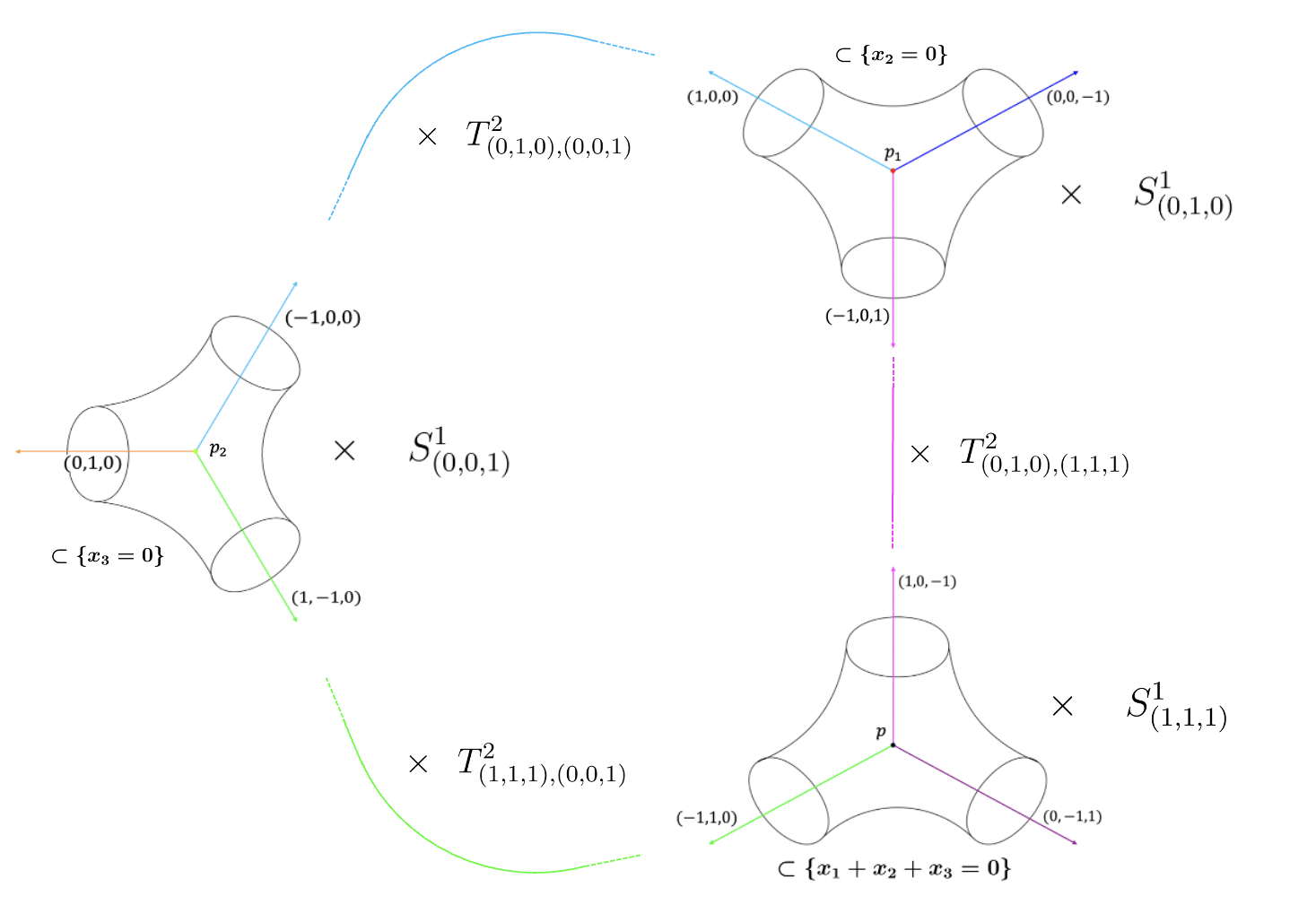
Figure 6. A representation of a part of the Lagrangian lift of $C$ inside $X(B)\cong B\times T^{3}$. Each of the pairs of pants is contained in a $2$-plane inside $B$ indicated on the figure, and $S^{1}_{(p_{1},p_{2},p_{3})}$ denotes the $S^{1}$-factor in the fibre direction generated by the line $(p_{1},p_{2},p_{3})$ in $(T^{*}B)_{b}$. Similarly, $T^{2}_{(p_{1},p_{2},p_{3}),(q_{1},q_{2},q_{3})}$ denotes the $2$-torus in a fibre generated by the linear span of the vectors $(p_{1},p_{2},p_{3})$ and $(q_{1},q_{2},q_{3})$ in $(T^{*}B)_{b}$.

The Lagrangian lift $L^{-}$ of $C^{-}$ is simply the image of $L$ by a global symplectomorphism. Indeed, $C^{-}$ is the image of $C$ by the automorphism $(-1)$ of $B$. Because $(-1)$ is tropical, the induced symplectomorphism on $T^{*}J(C)$ yields a symplectomorphism $\varphi^{-}$ of $T^{*}J(C)/T^{*}_{\mathbb{Z}}J(C)$. Notice $L$ and $L^{-}$ are not disjoint, therefore the Lagrangian Ceresa cycle is only immersed.

Although we know that the Ceresa cycle is nullhomologous 4.6, it may not yet be clear that the Lagrangian Ceresa cycle is. This fact will follow from our proof of Theorem 7.1 (see Remark 7.3), although we can already exhibit some supporting evidence. Tropically, $(-1)$ acts as $-\operatorname{Id}$ on $H_{1}(J(C);\mathbb{Z})$ and $T_{\mathbb{Z}}^{*}J(C)\cong H_{2}(F;\mathbb{Z})$, therefore it acts trivially on $H_{1}(J(C))\otimes H_{2}(F;\mathbb{Z})$. We know that this homology group contains $\hat{\phi}(\overline{C})$, and it will follow from the proof of Theorem 7.1 that it also contains $L$.

7.2. Main result

Here we prove the following Theorem:

Theorem 7.1.

For a generic tropical curve $C$ of type $K4$ with $g(C)=3$, the Lagrangian Ceresa cycle $L-L^{-}\in algCob^{or}(X(J(C)))_{hom}$ has infinite order.

From which the following Corollary is immediate from Remark 3.5:

Corollary 7.2.

For a generic tropical curve $C$ of type $K4$ with $g(C)=3$, the Lagrangian Ceresa cycle $L-L^{-}\in\mathcal{C}ob^{or}(X(J(C)))_{hom}$ has infinite order.

This result builds on Zharkov’s proof of the corresponding tropical statement 4.5 about the Ceresa cycle $C-C^{-}\in CH_{1}(J(C))$ being non-torsion. There Zharkov constructs a tropical $2$-chain $\gamma_{0}$ in $C_{2}(J(C),T_{\mathbb{Z}}B)$ satisfying $\partial\gamma_{0}=\overline{C}-\overline{C^{-}}$. He shows that

$$\int_{\gamma_{0}}\Omega^{3}_{1}=-ad,$$

which for a generic choice of edge lengths $\{a,b,c,d,e,f\}$ is not torsion modulo the period lattice computed in Example 5.5.

Recall from Example 6.4 that the determinantal form $\Omega^{3}_{1}$ is mapped through the appropriate choice of $\hat{\psi}$ to

$$\frac{1}{2}\omega^{2}\in\Omega^{2}(X(J(C))),$$

where $\omega$ is the canonical symplectic form on $X(J(C))$ induced by the one on $T^{*}J(C)$. Therefore by Proposition 6.2,

$$\int_{\gamma_{0}}\Omega^{3}_{1}=\frac{1}{2}\int_{\hat{\phi}(\gamma_{0})}\omega^{2}.$$

Proof of Theorem 7.1.

To prove Theorem 7.1, we apply Lemma 2.4 with $\alpha:=\frac{1}{2}\omega$, integrating $\frac{1}{2}\omega^{2}$ over an $n+1$-chain between $L$ and $L^{-}$. Notice that $\hat{\phi}(\gamma_{0})$ is an $(n+1)$-chain between $\hat{\phi}(\overline{C})$ and $\hat{\phi}(\overline{C^{-}})$, on which $\frac{1}{2}\omega^{2}$ integrates to something which is not in its periods. In Matessi’s construction of the Lagrangian pair-of-pants, he shows (Corollary 3.19 in [Mat21]) that these come in families which converge to his piecewise-linear Lagrangian lift. By inspection of [Mat21, Section 2] and by Section 6.4, the piecewise-linear Lagrangian lift of $C$ coincides with $\hat{\phi}(C)$. This family gives an $(n+1)$ chain $\gamma$ connecting $L$ and $\hat{\phi}(C)$, on which $\omega^{2}$ necessarily vanishes (as on any $(n+1)$-chain given by a $1$-dimensional family of Lagrangians). The same argument yields an $(n+1)$-chain $\gamma^{-}$ connecting $L^{-}$ and $\hat{\phi}(C^{-})$ on which $\omega^{2}$ vanishes. Therefore

$$\int_{\gamma\cup\hat{\phi}(\gamma_{0})\cup\gamma^{-}}\frac{1}{2}\omega^{2}=\int_{\hat{\phi}(\gamma_{0})}\frac{1}{2}\omega^{2}=\int_{\gamma_{0}}\Omega_{1}^{3}=-ad.$$

Because the maps $\phi$ and $\psi$ are isomorphisms, the periods of $\frac{1}{2}\omega^{2}$ are exactly the periods of $\Omega^{3}_{1}$. Therefore for a generic choice of edge lengths, $-ad$ is not torsion modulo the periods of $\frac{1}{2}\omega^{2}$, and we conclude. ∎

Remark 7.3.

While $\phi$ being an isomorphism already implied that $\hat{\phi}(C)$ and $\hat{\phi}(C^{-})$ are homologous, the $(n+1)$-chains provided by Matessi’s converging family of pairs-of-pants allows us to conclude that $L$ and $L^{-}$ are homologous in $X(J(C))$.

Remark 7.4.

While for generic choices of edge lengths, the flux $-ad$ is not torsion in $\mathcal{P}^{3}_{1}$, our computation 5.5 shows that choosing for instance $f=0$ immediately yields $-ad\in\mathcal{P}^{3}_{1}$. Although no analogous results have been brought to light tropically, classically [Bea21, BS23] exhibit an example of a non-hyperelliptic curve which nevertheless has torsion Ceresa cycle.

Remark 7.5.

It is worth noting that a few years after Ceresa proved the inifinite order statement for the Ceresa cycle in $\text{Griff}_{1}(J(C))$, Bardelli proved that this group is in fact infinitely generated. He proceeds by constructing generators as follows: for every $k\geq 1$, the cycles $C_{k}-C_{k}^{-}\in\text{Griff}_{1}(J(C))$ are pushforwards of Ceresa cycles of curves $C_{k}$ for which $J(C_{k})$ has a $k$-to-$1$ map to $J(C)$. It is expected that one could prove a similar statement symplectically, only with our methods this would require a tropical construction of these infinitely many generators, which to the best of our knowledge has not appeared in the literature. There has been, however, progress on the tropical Schottky problem; for instance an algorithm to produce a tropical curve $C_{k}$ from the data of its Jacobian (and a theta divisor) is suggested in [BBC17, Section 7], and in [CKS17].

7.3. Speculation for higher genus curves

While we have thus far restricted to studying the genus three $K4$ graph, we expect the methods used to be able to produce statements about Lagrangian Ceresa cycles of any higher genus tropical curve containing $K4$ as a subgraph.

Conjecture 7.1.

Let $C$ be a generic finite compact trivalent tropical curve of genus $\geq 3$ containing $K4$ as a subgraph. Then $L_{C}-L_{C}^{-}\in algCob^{or}(X(J(C)))$, its Lagrangian Ceresa cycle, has infinite order.

This Conjecture is motivated by the following tropical statement by Zharkov:

Theorem 7.6.

[Zha13, Theorem 8] Let $C$ be a generic tropical curve of genus $\geq 3$ containing $K4$ as a subgraph. Then $C$ is not algebraically equivalent to $C^{-}$ in $J(C)$.

The argument is sketched as follows. Let $C$ be a genus $g\geq 3$ curve containing $K4$ as a subgraph. We proceed by successively removing edges $e$ of $C$ to obtain a new curve $C_{e}$, until we are left with the $K4$ graph. Notice that this can be done in a way that at each iteration, $C_{e}$ is connected (up to removing edges which have constant image in the Jacobian). Furthermore, we only consider compact curves whose underlying graph is finite, therefore there are no $1$-valent vertices (this property is inherited by $C_{e}$ as two metric graphs are said to be equivalent if one is obtained from another by inserting a $2$-valent vertex in the interior of an edge). With these precautions, we observe that after each iteration $g(C_{e})=g(C)-1$. Zharkov proves [Zha13, Propositions 6. and 7.] that this comes with a tropical projection map $J(C)\rightarrow J(C_{e})$ along the direction of the edge $e$ in $J(C)$, which maps $C\subset J(C)$ to $C_{e}\subset J(C_{e})$. Because an algebraic equivalence between $C$ and $C^{-}$ would survive this tropical projection map, iterating this process would eventually lead to a contradiction.

A natural approach to proving a symplectic version of this would be the following. The graph of the tropical projection map above is a cycle of dimension $g$ in $J(C)\times J(C_{e})$, which induces a map

$$CH_{i}(J(C))\longrightarrow CH_{i}(J(C_{e})).$$

If we choose a set of coordinates $(x_{1},\dots,x_{g})$ for $J(C)$ such that the tangent vector to $e$ in $J(C)$ is parallel to $(0,\dots,0,1)$, then this $g$-cycle is

$$\{(x_{1},\dots,x_{g},x_{1},\dots,x_{g-1})\}\subset J(C)\times J(C_{e}).$$

Using the associated cotangent coordinates, this motivates us to consider its Lagrangian lift as a Lagrangian correspondence

$$P:=\{(x_{1},p_{1},\dots,x_{g},0,x_{1},p_{1},\dots,x_{g-1},p_{g-1})\}\subset\overline{X(J(C))}\times X(J(C_{e})).$$

Our result would follow from the following Conjecture:

Conjecture 7.2.

Let $Y$ be an oriented Lagrangian correspondence $Y\subset\overline{X}\times X^{\prime}$ between symplectic manifolds $X$ and $X^{\prime}$. Then $Y$ induces a well-defined map

$$Y: \hskip 2.84526ptalgCob(X)\longrightarrow algCob(X^{\prime})$$

$$\hskip 25.60747ptL\hskip 28.45274pt\mapsto\hskip 19.91692ptY(L).$$

One reason to expect and hope for this statement to be true, is that this would be the symplectic manifestation of the fact that algebraic equivalence is an adequate equivalence relation, in particular it behaves well under correspondences. A more explicit piece of evidence is hinted in the following Lemma:

Lemma 7.7.

Let $Y$ be an oriented Lagrangian correspondence $Y\subset\overline{X}\times X^{\prime}$ between symplectic manifold $X$ and $X^{\prime}$ which satisfies $\pi_{X}(Y)=X$. Then $Y$ induces a well-defined map

$$Y: \hskip 2.84526ptalgCob(X)\longrightarrow algCob(X^{\prime})$$

$$\hskip 25.60747ptL\hskip 28.45274pt\mapsto\hskip 19.91692ptY(L).$$

Proof.

Let $L_{1}$ and $L_{2}$ be oriented Lagrangians in $X$. Assume there is an oriented Lagrangian correspondence

$$\Gamma:L_{1}\stackrel{{\scriptstyle A_{p,q}}}{{\rightsquigarrow}}L_{2},$$

and set $L^{\prime}_{i}:=Y(L_{i})$ for $i=1,2$. Denote by $\Delta_{A}\subset\overline{A}\times A$ be the diagonal, and by

$$\varphi_{1324}: \hskip 2.84526ptX\times X^{\prime}\times A\times A\longrightarrow X\times A\times X^{\prime}\times A$$

$$\hskip 8.53581pt(x_{1},x_{2},x_{3},x_{4})\hskip 12.80373pt\mapsto\hskip 11.38109pt(x_{1},x_{3},x_{2},x_{4})$$

the map interchanging the factors. Then $\varphi_{1324}(Y\times\Delta_{A})$ is an oriented Lagrangian correspondence between $X\times A$ and $X^{\prime}\times A$. Define $\Gamma^{\prime}\subset X^{\prime}\times A$ as the image of $\Gamma$ under this correspondence. Observe

$$\Gamma^{\prime}(F_{q}) =\pi_{X^{\prime}}(\Gamma^{\prime}\pitchfork(X^{\prime}\times F_{q}))=\pi_{X^{\prime}}(\varphi_{1324}(Y\times\Delta_{A})\pitchfork(X^{\prime}\times F_{q}))$$

$$=\pi_{X^{\prime}}\left(\pi_{X^{\prime}\times A}(\varphi_{1324}(Y\times\Delta_{A})\pitchfork(\Gamma\times X^{\prime}\times A)\pitchfork(X^{\prime}\times F_{q}))\right)$$

$$=\pi_{X^{\prime}}\left(\varphi_{1324}(Y\times\Delta_{A})\pitchfork(\Gamma\times X^{\prime}\times F_{q})\right)=L^{\prime}_{2}.$$

Similarly, we have $\Gamma^{\prime}(F_{p})=L_{1}^{\prime}$. Finally, we verify that $\pi_{B}(\Gamma^{\prime})=B$, in other words that $\forall b\in B$, $\Gamma^{\prime}(F_{b})$ is non-empty. This can be rephrased as the requirement that for all $b\in B$, there should exist an $x\in X$, an $x^{\prime}\in X^{\prime}$, and an $f\in F_{b}$ such that $(x,x^{\prime})\in Y$ and $(x,f)\in\Gamma$. We know that $\pi_{B}(\Gamma)=B$, therefore we are guaranteed the existence of some $x\in X$ and $f\in F_{b}$ such that $(x,f)\in\Gamma$. The existence of an associated $x^{\prime}\in X^{\prime}$ such that $(x,x^{\prime})\in Y$ follows from our condition that $\pi_{X}(Y)=X$. ∎

Here the condition that $\pi_{X}(Y)=X$ is used to ensure that $\pi_{B}(\Gamma^{\prime})=B$. Very generally, we expect that this condition can be relaxed while still yielding an equivalent definition for algebraic Lagrangian cobordisms. Recall from Section 3.1 that the classical notion of algebraic equivalence can be equivalently formulated in terms of cycles living in flat families over a curve, an abelian variety, or any smooth projective variety [ACV16]. It is reasonable to expect a similar statement tropically, and by extension for our definition of algebraic Lagrangian cobordisms to be equivalent to the existence of a Lagrangian correspondence $\Gamma^{\prime}$ supported on a tropical curve for instance, as in Lemma 3.7.

Notice that in our specific setting of the correspondence $P\subset\overline{X(J(C))}\times X(J(C_{e}))$ above, the condition $\pi_{B}(P)$ fails to be satisfied in a very tangible way. Namely, letting $H:=\{p_{g}=0\}$ be the hyperplane $p_{g}=0$ in $X(J(C))$,

$$\pi_{B}(P)=\pi_{B}(\Gamma\cap(H\times A)),$$

which generically has dimension $\dim(B)+g-1\geq\dim(B)$.

8. Some additional remarks

8.1. Tropical curves of hyperelliptic type

The failure of the tropical Torelli theorem implies that some non-hyperelliptic curves can have a Jacobian isomorphic to that of a hyperelliptic curve; these are said to be of hyperelliptic type. Readers are referred to [Cha13] for background on tropical hyperelliptic curves, and [Cor21] for background on tropical curves of hyperelliptic type. In the latter, it is shown that a curve being of hyperelliptic type depends only on its underlying graph.

Throughout this paper, we have been concerned with a genus $3$ tropical curve of type $K4$ as represented in 2. There are however, four additional types of generic genus $3$ tropical curves; see Figure 7. By generic we mean that all other genus three tropical curves can be obtained as degenerations of these (in particular they are trivalent).

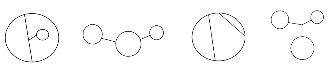
Figure 7. The four generic types of genus three tropical curves of hyperelliptic type.

The curves from Figure 7 are of hyperelliptic type. Figure 8 gives an example of two curves which have isomorphic Jacobians, yet the one on the left is hyperelliptic while the one on the right isn’t.

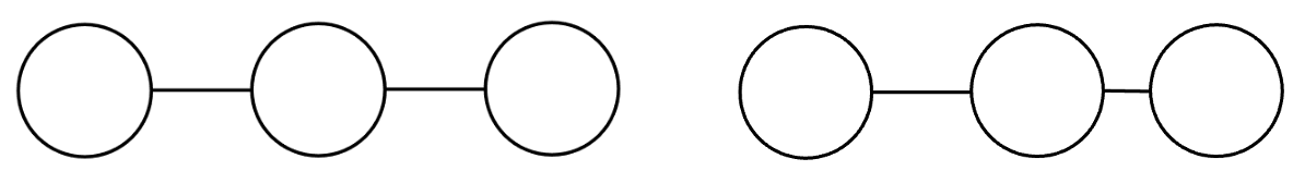
Figure 8. Two curves with isomorphic Jacobians, however the left one is hyperelliptic and the right one isn’t.

Recently, C. Ritter has shown [Rit24, Theorem A.] that, if $C$ is any genus $g$ tropical curve, the $\Omega^{g}_{1}$-flux obstruction for its Ceresa cycle $C-C^{-}$ vanishes if and only if $C$ is of hyperelliptic type. In particular, this implies that the symplectic flux vanishes for the Lagrangian Ceresa cycles associated to curves of hyperelliptic type. However, the mirror correspondence between rational equivalence and Lagrangian cobordisms suggests that they are not generally nullcobordant. These limitations of flux as an obstruction to Lagrangian cobordisms could already be noticed from the fact that it does not allow us to detect Lagrangians which are oriented cobordant, but not unobstructed cobordant.

8.2. Flux and characters of symplectic Torelli-type groups

A concept closely related to our notion of symplectic flux appeared in a paper by Reznikov [Rez97, Section 4], where it is used to construct characters of a symplectic Torelli-type group $Symp_{0}(X)/Ham(X)$. Here $Symp_{0}(X)$ is the kernel of the map

$$Symp(X)\longrightarrow\operatorname{Aut}(H_{odd}(X;\mathbb{Z})),$$

and $Ham(X)\subset Symp(X)$ is the subgroup of Hamiltonian isotopies of $X$.

Given $f\in Symp_{0}(X)$ and $z\in H_{2k-1}(X;\mathbb{Z})$, define

$$\chi(f,z):=\int_{b}\omega^{k}\mod\mathbb{Z},$$

with $b$ is a $2k$-chain satisfying $\partial b=c-f(c)$, and $c$ a chain representing $z$. This yields a well-defined map [Rez97, Theorem 4.1]:

$$\chi:Symp_{0}(X)/Ham(X)\longrightarrow\hom(H_{odd}(X;\mathbb{Z}),\mathbb{R}/\left([\omega^{k}]\cdot H_{2k}(X;\mathbb{Z})\right).$$

Now let $X$ be a symplectic manifold of dimension $2(2k-1)$, and fix a class $z\in H_{2k-1}(X;\mathbb{Z})$ which admits a Lagrangian representative $L$. Then

$$\chi(\cdot,z):Symp_{0}(X)/Ham(X)\longrightarrow\mathbb{R}/\left([\omega^{k}]\cdot H_{2k}(X;\mathbb{Z})\right)$$

fits into a commutative diagram

From this perspective, Theorem 7.1 can be translated into a non-triviality result for Reznikov’s character in $X(J(C))$. Indeed, recall that $L^{-}=\varphi^{-}(L)$ for some global symplectomorphism $\varphi^{-}$ which is in $Symp_{hom}(X)$. However, it is important to notice that the horizontal map from $Symp_{hom}(X)/Ham(X)$ to $Cob^{or}(X)_{hom}$ is not a group homomorphism, but a crossed homomorphism satisfying

$$\varphi_{2}\circ\varphi_{2}\mapsto(L-\varphi_{1}(L))+(\varphi_{1}(L)-\varphi_{2}\circ\varphi_{1}(L)).$$

In particular, in the case of the Ceresa cycle, $\varphi^{-}$ is of order two, and is mapped to $L-L^{-}$ of infinite order in $\mathcal{C}ob^{or}(X(J(C)))_{hom}$.

References

- [AWe54] A.Weil “Sur les critères d’équivalence en géométrie algébrique” In Math. Ann. 128, 1954, pp. 95–127
- [Abo08] Mohammed Abouzaid “On the Fukaya categories of higher genus surfaces” In Advances in Mathematics 217.3, 2008, pp. 1192–1235
- [ACV16] Jeff Achter, Sebastian Casalaina-Martin and Charles Vial “Parameter spaces for algebraic equivalence” In arXiv: Algebraic Geometry, 2016 URL: https://api.semanticscholar.org/CorpusID:119307498
- [Ale+08] Valery Alexeev, Arnaud Beauville, C. Clemens and Elham Izadi “Curves and Abelian Varieties” 465, Contemporary Mathematics American Mathematical Society, 2008
- [AR10] Lars Allermann and Johannes Rau “First Steps in Tropical Intersection Theory” In Mathematische Zeitschrift 264.3, 2010, pp. 633–670
- [Arn80] V.. Arnol’d “Lagrange and Legendre Cobordisms. I” In Functional Analysis and Its Applications 14.3, 1980, pp. 167–177
- [Bea21] Arnaud Beauville “A Non-Hyperelliptic Curve with Torsion Ceresa Class” In Comptes Rendus. Mathématique 359.7, 2021, pp. 871–872
- [BS23] Arnaud Beauville and Chad Schoen “A Non-Hyperelliptic Curve with Torsion Ceresa Cycle Modulo Algebraic Equivalence” In International Mathematics Research Notices 2023.5, 2023, pp. 3671–3675
- [BC13] Paul Biran and Octav Cornea “Lagrangian Cobordism. I” In Journal of the American Mathematical Society 26.2 American Mathematical Society, 2013, pp. 295–340 JSTOR: 43302800
- [BC14] Paul Biran and Octav Cornea “Lagrangian Cobordism and Fukaya Categories” In Geometric and Functional Analysis 24.6, 2014, pp. 1731–1830
- [Blo] Spencer Bloch “Some elementary theorems about algebraic cycles on abelian varieties” In Inventiones Mathematicae
- [BBC17] Barbara Bolognese, Madeline Brandt and Lynn Chua “From Curves to Tropical Jacobians and Back”, 2017 arXiv: https://arxiv.org/abs/1701.03194
- [Bos24] Valentin Bosshard “Lagrangian Cobordisms in Liouville Manifolds” In Journal of Topology and Analysis 16.05, 2024, pp. 777–831
- [Cer83] G. Ceresa “C Is Not Algebraically Equivalent to C- in Its Jacobian” In Annals of Mathematics 117.2 Annals of Mathematics, 1983, pp. 285–291
- [Cha13] Melody Chan “Tropical Hyperelliptic Curves” In J. Algebraic Comb. 37.2, 2013, pp. 331–359
- [CL24] Jean-Philippe Chassé and Rémi Leclercq “Weinstein exactness of nearby Lagrangians and the Lagrangian flux conjecture”, 2024 arXiv:2410.04158 [math.SG]
- [Che96] Yu.. Chekanov “Lagrangian tori in a symplectic vector space and global symplectomorphisms” In Mathematische Zeitschrift 223, 1996, pp. 547–559
- [CKS17] Lynn Chua, Mario Kummer and Bernd Sturmfels “Schottky algorithms: Classical meets tropical” In Math. Comput. 88, 2017, pp. 2541–2558
- [Cle83] Herbert Clemens “Homological Equivalence, modulo Algebraic Equivalence, Is Not Finitely Generated” In Publications Mathématiques de l’Institut des Hautes Études Scientifiques 58.1, 1983, pp. 19–38
- [Cor21] Daniel Corey “Tropical Curves of Hyperelliptic Type” In Journal of Algebraic Combinatorics 53.4, 2021, pp. 1215–1229
- [CEL23] Daniel Corey, Jordan Ellenberg and Wanlin Li “The Ceresa class: tropical, topological and algebraic” In Journal of the Institute of Mathematics of Jussieu, 2023, pp. 1–41
- [CL24a] Daniel Corey and Wanlin Li “The Ceresa Class and Tropical Curves of Hyperelliptic Type” In Forum of Mathematics, Sigma 12, 2024
- [Eva22] Jonathan David Evans “Lectures on Lagrangian Torus Fibrations” arXiv, 2022 arXiv:2110.08643 [math]
- [Fuk02] Kenji Fukaya “Floer Homology for Families – A Progress Report” In Integrable systems, topology, and physics (Tokyo, 2000), 2002
- [Ful] William Fulton “Intersection Theory”
- [Gil05] Henri Gillet “K-Theory and Intersection Theory” In Handbook of K-Theory Berlin, Heidelberg: Springer, 2005, pp. 235–293
- [Hau15] Luis Haug “The Lagrangian Cobordism Group of $$T^2$$ T 2” In Selecta Mathematica, 2015, pp. 1021–1069
- [Hau20] Luis Haug “Lagrangian Antisurgery” In Mathematical Research Letters 27.5, 2020, pp. 1423–1464
- [Hic22] Jeff Hicks “Wall-Crossing from Lagrangian Cobordisms”, 2022 arXiv:1911.09979 [math]
- [HM22] Jeffrey Hicks and C. Mak “Some Cute Applications of Lagrangian Cobordisms towards Examples in Quantitative Symplectic Geometry”, 2022
- [Ite+19] Ilia Itenberg, Ludmil Katzarkov, Grigory Mikhalkin and Ilia Zharkov “Tropical Homology” 42 PAGES, 1 figure, introduction expanded and references added, publication status added In Mathematische Annalen Springer Verlag, 2019
- [KS04] Maxim Kontsevich and Yan Soibelman “Affine Structures and Non-Archimedean Analytic Spaces”, 2004 arXiv:math/0406564
- [Lan83] Serge Lang “Abelian varieties” Springer, 1983
- [MR20] Cheuk Yu Mak and Helge Ruddat “Tropically Constructed Lagrangians in Mirror Quintic Threefolds” In Forum of Mathematics, Sigma 8, 2020, pp. e58 arXiv:1904.11780 [math]
- [Mat21] Diego Matessi “Lagrangian Pairs of Pants” In International Mathematics Research Notices 2021.15, 2021, pp. 11306–11356
- [Mik19] Grigory Mikhalkin “Examples of Tropical-to-Lagrangian Correspondence”, 2019 arXiv:1802.06473 [math]
- [MZ08] Grigory Mikhalkin and Ilia Zharkov “Tropical Curves, Their Jacobians and Theta Functions” In Contemporary Mathematics 465 Providence, Rhode Island: American Mathematical Society, 2008, pp. 203–230
- [MR] Mikhalkin, Grigory and Rau, Johannes “Tropical Geometry”
- [Muñ24] Álvaro Muñiz-Brea “Lagrangian Cobordisms and K-theory of Symplectic Bielliptic Surfaces”, 2024 arXiv:2403.17098 [math]
- [Rat23] Dominique Rathel-Fournier “Unobstructed Lagrangian Cobordism Groups of Surfaces”, 2023 arXiv:2307.03124 [math]
- [Rez97] A.G. Reznikov “Characteristic Classes in Symplectic Topology” In Selecta Mathematica 3.4, 1997, pp. 601–642
- [Rit24] Caelan Ritter “The Ceresa Period from Tropical Homology”, 2024 arXiv:2405.07402 [math]
- [Sei08] Seidel Paul “Fukaya Categories and PIcard-Lefschetz Theory” European Mathematical Society, 2008
- [SS20] Nick Sheridan and Ivan Smith “Rational Equivalence and Lagrangian Tori on K3 Surfaces” In Commentarii Mathematici Helvetici 95.2, 2020, pp. 301–337 arXiv:1809.03892 [math]
- [SS20a] Nick Sheridan and Ivan Smith “Symplectic Topology of K3 Surfaces via Mirror Symmetry” In Journal of the American Mathematical Society 33.3, 2020, pp. 875–915 arXiv:1709.09439 [math]
- [SS21] Nick Sheridan and Ivan Smith “Lagrangian Cobordism and Tropical Curves” In Journal für die reine und angewandte Mathematik (Crelles Journal) 2021.774 De Gruyter, 2021, pp. 219–265
- [Ste43] N.. Steenrod “Homology With Local Coefficients” In The Annals of Mathematics 44.4, 1943, pp. 610 JSTOR: 1969099
- [Sub10] Aleksandar Subotic “A monoidal structure for the Fukaya category”, 2010
- [Zha13] Ilia Zharkov “$C$ Is Not Equivalent to $C^-$ in Its Jacobian: A Tropical Point of View”, 2013 arXiv:1305.4595 [math]