Can optimal diversification beat the naive $1/N$ strategy in a highly correlated market? Empirical evidence from cryptocurrencies

Abstract

This study systematically examines how several alternative approaches considered affect three aspects that determine portfolio performance (the gross return, the transaction costs and the portfolio risk). We find that it is difficult to exploit the possible predictability of asset returns. However, the predictability of asset return volatility produces obvious economic value, although in a highly correlated cryptocurrencies market.

Keywords: mean-variance analysis, conditional mean, conditional variance, turnover penalty, performance fee.

1 Introduction

1.1 Related literature

Since the Markowitz’s modern portfolio theory was proposed in 1952, it has attracted extensive attention from both academia and financial industry. However, in many practical applications, Markowitz rule and its variants even perform worse than the equally weighted naive diversification. Michaud (1989) explains this tendency by the “error-maximizing” property of the mean-variance optimization, which suggests that the error in estimating risk and return leads to poor performance. Under the assumption that excess return follows a multivariate normal distribution, by using an expected loss function in the standard mean-variance analysis context, Kan and Zhou (2007) show analytically that the classical plug-in method using sample estimates to replace true parameters in optimization problem can result in poor out-of-sample performance. Under the same assumption, DeMiguel et al. (2009) indicate that a minimum length of estimation window is required such that standard mean-variance strategy can outperform the $1/N$ strategy, due to the existence of parameter uncertainty or estimation error.

As estimation error is one of the main causes of poor performance generated by optimal diversification, how to address estimation error has become a significant issue. In fact, there has been a large literature devoted to this issue in academia. For instance, DeMiguel et al. (2009) evaluate the performance of standard mean-variance model and its 13 extensions, covering almost all prominent models proposed in prior literature to mitigate the impact of estimation error. Most of these extensions employ the Bayesian or various shrinkage approaches, and the rest impose certain restrictions on the estimated moments. Nevertheless, according to the empirical results, DeMiguel et al. (2009) report that none of the considered models can consistently outperform the naive diversification for seven empirical datasets, which issue a serious challenge to the usefulness of portfolio theory. Fortunately, by using the shrinkage estimator toward $1/N$, Tu and Zhou (2011) develop an combination rule that optimally combines the $1/N$ weights with the weights obtained from each of four sophisticated rules derived from investment theory, and find that all of them outperform both the original sophisticated rules and the naive $1/N$ rule. This result seems to vindicate the mean-variance theory. Furthermore, Kirby and Ostdiek (2012) revisit the DeMiguel et al. (2009) results and indicate that the poor performance is largely due to their research design, which places the mean-variance optimization at an inherent disadvantage. By setting the conditional expected return equals to that of $1/N$ rule, the mean-variance model can outperform the $1/N$ rule for most of DeMiguel et al. (2009) datasets when transaction costs are not taken into account. In the presence of transaction costs, Kirby and Ostdiek (2012) also propose two new timing strategies dominating naive diversification, which mitigates estimation error by exploiting solely the estimated conditional volatility or estimated reward-to-risk ratios.

As can be seen, most of aforementioned studies primarily focus on improving the misspecification of the first two moments of asset returns through statistical analysis under the assumption of normality, while Kirby and Ostdiek (2012) effectively implement a new perspective of time-varying moments. There has been ample empirical evidence suggesting time-vary asset return moments (Gao and Nardari, 2018). A considerable amount of asset allocation literature adopts the time-varying perspective, with some studies focusing on volatility timing (see, e.g. Fleming et al. (2001) and Fleming et al. (2003)), others emphasizing return forecasting (see, e.g. Ahmed et al. (2016), Opie and Riddiough (2020)) , and most concerning with both matters (see, e.g., Della Corte et al. (2009), Kirby and Ostdiek (2012) and Gao and Nardari (2018)). Recent years, there has been a growing body of asset allocation literature employing machine learning techniques for return forecasting (see, e.g. D’Hondt et al. (2020), Chen et al. (2021), Ma et al. (2021), Kynigakis and Panopoulou (2022) and Du (2022)).

However, in the real world, any gains from optimal diversification can be easily eroded by large transaction costs. In traditional mean-variance optimization problem, the gains obtained from a rebalancing may not compensate the costs required for a rebalancing. As a result, it becomes necessary to introduce transaction costs into the optimization problem. Yoshimoto (1996) propose an optimization system with V-shaped cost function, and the empirical results show that ignoring transaction costs results in the higher turnover and an inefficient portfolio. Olivares-Nadal and DeMiguel (2018) theoretically and empirically explore the role of transaction costs in portfolio optimization problem. They prove that the mean-variance problem with p-norm transaction costs is equivalent to three different problems designed to deal with the estimation error: a robust portfolio problem, a regularized linear regression problem, and a Bayesian portfolio problem. The data-driven approach proposed by Olivares-Nadal and DeMiguel (2018) also typically outperform the benchmark portfolio, because it addresses transaction costs and estimation error simultaneously. Similarly, Hautsch and Voigt (2019) first theoretically demonstrate that the regulatory effect of quadratic and proportional transaction costs. Then an extensive empirical study in a large-scale portfolio optimization framework shows that the ex ante incorporation of transaction costs is crucial for achieving a reasonable portfolio performance.

In light of the aforementioned literature, we consider several alternative methods with regard to three areas of portfolio optimization problem in a conditional mean-variance context: the conditional mean, the conditional covariance and the objective function. For the conditional mean estimation, in addition to the conventional sample mean, we also consider the probabilistic time series forecasting based on state-of-the-art deep learning method. For the conditional covariance estimation, in addition to the conventional sample covariance, we also employ a DCC-EGARCH model to capture the volatility dynamics. For the objective function, we consider incorporating a turnover penalty term to inhibit excessive rebalancing.

Particularly, for the conditional mean estimation, we consider a special case where all the conditional means are set to be zero (i.e. the global minimum variance portfolio). DeMiguel et al. (2009) find that the minimum-variance strategy successfully reduce the extreme weights and the turnover of portfolio relative to the mean-variance strategy. Olivares-Nadal and DeMiguel (2018) also observe that the minimum-variance strategy generally outperform the mean-variance strategy, which they explain by the difficulties in estimating mean returns. Following numerous studies employing daily data, Hautsch and Voigt (2019) also ignore the estimation of mean returns but perform the minimum-variance strategy. Consequently, we consider a total of four optimization objective functions, depending on whether turnover penalty is incorporated and whether conditional mean is utilized. To the best of our knowledge, this is the first study that comprehensively examines the impacts of deep learning approaches, multivariate GARCH model, objective function with turnover penalty/zero conditional mean and rebalancing frequency on portfolio performance.

We employ cryptocurrencies as the empirical dataset of this paper to examine the performance of aforementioned strategies. As an emerging asset class, cryptocurrencies have widely attracted interest from investors, regulators and academia. Platanakis et al. (2018) implement an empirical examination employing weekly data of four popular cryptocurrencies, and conclude that there is no significant difference between the 1/N rule and the sample-based mean-variance strategy in cryptocurrency market. Over the past few years, cryptocurrencies have exhibited high correlations with each other. Generally, a lower level of correlation implies greater diversification benefits, and Christoffersen et al. (2014) propose a correlation-based measure of conditional diversification benefits where both parties are negatively related. DeMiguel et al. (2009) also indicate that optimal diversification can only outperform the naive 1/N strategy with very high idiosyncratic volatility through simulations. It appears that there are little diversification benefits in a highly correlated cryptocurrency market. However, from a contrary perspective, if a strategy can outperform the naive 1/N strategy in such a context, it would perform more robustly in other scenarios. This explains our interest in this matter.

1.2 Contribution and preview

This study contributes to the literature on portfolio optimization primarily in the following aspects:

First, we emphasize the impact of different estimators’ variation levels, which measure the variation characteristic of a series between before and after time, rather than measure the variation around average like variance. Most previous studies only involve the forecasting accuracy of estimators (see, e.g., D’Hondt et al. (2020), Chen et al. (2021), Ma et al. (2021) and Du (2022)). However, Fleming et al. (2001) find that volatility timing shows better effectiveness with smoother covariance estimates than with those obtained from the minimum MSE criterion. Fleming et al. (2003) observe that volatile multivariate GARCH estimates lead to poor performance of volatility timing as well. Kirby and Ostdiek (2012) consider an alternative estimator of conditional means with a lower asymptotic variance, which reduces portfolio variance and turnover. In this study, we are more concerned with transaction costs incurred by mutable characteristic than with portfolio variance, so we evaluate different estimators using the variation level rather than variance.

Second, given numerous theoretical and empirical benefits of the turnover penalty (Yoshimoto, 1996; Olivares-Nadal and DeMiguel, 2018; Hautsch and Voigt, 2019), we incorporate a transaction cost term into the objective function of optimization problem. Furthermore, we examine the role of rebalancing frequency in the impact of turnover penalty on portfolio performance from a theoretical perspective. Despite the differences in analytical framework, our finding corresponds to the deduction in Woodside-Oriakhi et al. (2013) (the expected portfolio return per period is given by the weighted sum of asset returns, minus the transaction cost scaled by investment horizon H), which suggests that the impact of introducing transaction cost diminishes as H increases.

Third, we adopt the larger one of two analytical solutions for performance fee as our evaluation criteria in accordance with Kirby and Ostdiek (2012) and detail the economic implication of performance fee to justify our choice. We highlight this because employing some software packages directly might yield the smaller solution which is unreasonable according to economic implication. Furthermore, we explicitly show that higher return and lower risk than the benchmark strategy facilitate generating positive performance fee. Given the performance of benchmark model, higher return and lower risk facilitate generating greater performance fee. Besides, return plays a more significant role than risk in determining performance fee.

Fourth, instead of focusing solely on eventual evaluation metrics, we detail the impact of various alternative methods on several aspects that determine portfolio performance. Most previous studies focus on eventual performance metrics (see, e.g., DeMiguel et al. (2009), Della Corte et al. (2009), Gao and Nardari (2018), Ahmed et al. (2016) and Opie and Riddiough (2020)). On a risk-adjusted basis, the portfolio performance is determined by return and risk, where the return net of transaction costs is further decomposed into the gross return and the transaction costs. Accordingly, we systematically analyze how various alternative methods considered in this study impact these three aspects that determine portfolio performance (the gross return, the transaction costs, the risk).

To preview our results:

(I) Depending solely on historical data (deep learning models train parameters using a “cross-learning” approach), deep learning models cannot produce more accurate forecasts than sample means and the errors are even slightly larger, which is similar to the results of Makridakis et al. (2023). However, on the other hand, the predictability of asset return volatility obviously improves portfolio risk, regardless of in the volatility timing or mean-variance context.

(II) We find that the estimators obtained from sophisticated methods (deep learning forecasts, DCC covariances) tend to be more volatile than their sample counterparts and usually lead to poor performance. Since the performance of moment estimation relies not only on the forecasting accuracy, but also on the variation level, especially for conditional mean estimation. With similar forecasting accuracy, the one with lower variation level is preferred. A higher variation level tends to result in larger transaction costs and higher portfolio risk, which deteriorate portfolio performance. Our finding coincides with and enhances the discussions in Fleming et al. (2001), Fleming et al. (2003), Kirby and Ostdiek (2012) and Kynigakis and Panopoulou (2022).

(III) The empirical results justify the significance of turnover penalty in reducing transaction costs and improving performance under a mean-variance context, which is consistent with Yoshimoto (1996) and Olivares-Nadal and DeMiguel (2018). For volatility timing strategies, the portfolios using DCC covariances are obviously improved and achieve comparable performance to those using sample estimates, which extends the finding in Fleming et al. (2001) and Fleming et al. (2003). Nevertheless, our turnover penalty ($L_{1}$-norm) isn’t beneficial for the portfolios using sample covariances, which effectively corresponds to the results of shortsale-constrained minimum-variance portfolio with nominal transaction costs in Olivares-Nadal and DeMiguel (2018). Furthermore, our analytical derivation suggests that the improvement resulting from turnover penalty will diminish as the rebalancing frequency decreases, which is similar to Woodside-Oriakhi et al. (2013), and our empirical results also confirm this.

(IV) Even in highly correlated cryptocurrency market, most of the volatility timing portfolios achieve positive performance fees and obviously outperform their counterparts depending on return estimates, which justifies the economic value of predictability of asset return volatility. Even after the turnover penalty is imposed, the portfolios utilizing return estimates are also inferior to those volatility timing portfolios and the naive 1/N benchmark, which reconfirms that it’s difficult to capture the possible predictability of asset return in order to produce investment gains.

The remainder of this paper is organized as follows. Section 2 introduces four optimization frameworks employed in this study and analytically derive the role of rebalancing frequency. Section 3 presents the methodology for estimating conditional moments of asset returns and dataset used in this study. Section 4 describes the optimization modelling process and various performance measures. Section 5 reports and demonstrates the empirical results for daily and weekly rebalancing cases. Section 6 concludes.

2 Optimization frameworks

In this section, we describe four different optimization frameworks for deriving optimal portfolio weights and discuss the regularization effect introduced by turnover penalty.

2.1 The MV and the MVC optimization

Based on the existing studies aforementioned, we abandon the assumption of constant moments and normality in this study and consider the conditional mean-variance optimization approach (“MV” optimization, hereafter) like in Della Corte et al. (2009) and Kirby and Ostdiek (2012):

$$\underset{w_{t}}{min}\;\{\frac{\gamma}{2}w_{t}^{\prime}\Sigma_{t+1|t}w_{t}-w_{t}^{\prime}\mu_{t+1|t}\}$$ (1)

$$s.t.\;w_{t}^{\prime}l=1$$

where $w_{t}$ is the N-dimensional decision variable representing the optimal portfolio weights derived at time t, $\mu_{t+1|t}$ and $\Sigma_{t+1|t}$ are the conditional mean and the conditional covariance matrix of N risk asset returns during the period from time t to time t+1 given the information set $I_{t}$ respectively, $l$ is a $N\times 1$ vector of ones, and $\gamma$ is the coefficient of relative risk aversion. In this study, we examine the portfolio performance using the risk aversion coefficients from 1 to 10 for all optimal strategies, where the “strategy” refers to a specific combination of mean estimator, covariance estimator and optimization framework, or the naive 1/N rule.

Given numerous theoretical and empirical benefits of the turnover penalty, we consider the second optimization framework incorporating transaction costs into the objective function (“MVC” optimization, hereafter). Olivares-Nadal and DeMiguel (2018) argue that the quadratic transaction costs ($L_{2}$-norm) might be more suitable to handle estimation error than the proportional transaction costs ($L_{1}$-norm), although the latter is more realistic. However, they also point out that if there are no estimation error, then proportional transaction costs are actually optimal. In this study, we want to examine whether our alternative approaches improve the forecasting accuracy of conditional moments, and hence we consider the MVC optimization framework with the proportional transaction costs as follows:

$$\underset{w_{t}}{min}\;\{\frac{\gamma}{2}w_{t}^{\prime}\Sigma_{t+1|t}w_{t}+\beta||w_{t}-w_{t-1^{+}}^{*}||_{1}-w_{t}^{\prime}\mu_{t+1|t}\}$$ (2)

$$s.t.\;w_{t}^{\prime}l=1$$

where $\beta=0.005$ represents the proportional transaction costs of 50 basis points for each of the risky assets (DeMiguel et al., 2009), $w_{t-1^{+}}^{*}$ denotes the vector of portfolio weights before rebalancing at time t (the initial value is set to $\vec{0}$), and the term $\beta||w_{t}-w_{t-1^{+}}^{*}||_{1}$ represents the transaction costs for rebalancing at time t. It is noticeable that the asset prices have changed during the period from time t to time t+1, and thus $w_{t-1^{+}}^{*}$ differs from the wights by which portfolio was rebalanced at time t-1 (i.e. optimal portfolio wights derived by optimization framework at time t-1, namely $w_{t-1}^{*}$). Formally, $w_{t-1^{+}}^{*}=(w_{1,t-1^{+}}^{*},\cdots,w_{i,t-1^{+}}^{*},\cdots,w_{N,t-1^{+}}^{*})$ with $w_{i,t-1^{+}}^{*}$ representing the portfolio weight in asset i before rebalancing at time t and can be written as:

$$w_{i,t-1^{+}}^{*}=\frac{(1+r_{i,t})^{\prime}w_{i,t-1}^{*}}{\sum_{i=1}^{N}(1+r_{i,t})^{\prime}w_{i,t-1}^{*}},\ \forall i.$$ (3)

where $r_{i,t}$ is the return in asset i during the period from time t-1 to time t, and $w_{i,t-1^{+}}^{*}$ is defined as above. In the MVC optimization framework, transaction costs are subtracted from the objective function, and hence potential penalties are automatically taken into account when rebalancing portfolio. Proposition 1 shows that the regularization effect resulting from turnover penalty varies with the rebalancing frequency.

Proposition 1.

The MVC optimization framework is equivalent to the classical mean-variance optimization problem with

$$\underset{w_{t}}{min}\;\{\frac{\gamma}{2}w_{t}^{\prime}\Sigma_{t+1|t}w_{t}-w_{t}^{\prime}\tilde{\mu}_{t|t+1}\}$$ (4)

$$s.t.\;w_{t}^{\prime}l=1$$

where $\tilde{\mu}_{t|t+1}=\mu_{t+1|t}-\beta g^{*}$, and $g^{*}$ is the subgradient vector of function $||w_{t}-w_{t-1^{+}}^{*}||_{1}$ evaluated at $w_{t}^{*}$.

As shown in Proposition 1, the turnover penalty in the MVC optimization framework imply a regularization effect shifting the conditional mean by $\beta g^{*}$. Since $g^{*}$ is bounded by $\pm 1$, the lower the rebalancing frequency, the smaller $\beta g^{*}$ will be relative to $\mu_{t+1|t}$, and hence the smaller the change caused by the turnover penalty will be. Intuitively, this also makes sense, since the lower the rebalancing frequency, the smaller the influence of transaction costs, corresponding with Woodside-Oriakhi et al. (2013).

2.2 The GMV and the VC optimization

Since the impact of estimation error is largely due to the error in mean estimation (DeMiguel et al., 2009), we consider two optimization frameworks which relies solely on the conditional covariance estimates. The first one is just the global minimal variance portfolio (“GMV” optimization, hereafter).

$$\underset{w_{t}}{min}\;\{\frac{\gamma}{2}w_{t}^{\prime}\Sigma_{t+1|t}w_{t}\}$$ (5)

$$s.t.\;w_{t}^{\prime}l=1$$

Due to the potential variation characteristic of covariance estimator, we also consider the influence of turnover penalty and propose the variance-cost optimization framework (“VC” optimization, hereafter) for portfolio choice, similar to that in Olivares-Nadal and DeMiguel (2018).

$$\underset{w_{t}}{min}\;\{\frac{\gamma}{2}w_{t}^{\prime}\Sigma_{t+1|t}w_{t}+\beta||w_{t}-w_{t-1^{+}}^{*}||_{1}\}$$ (6)

$$s.t.\;w_{t}^{\prime}l=1$$

The VC optimization framework minimizes the sum of risk (volatility) and transaction costs without utilizing the estimate of conditional mean, and thus will not influenced by the estimation error in conditional mean. Hautsch and Voigt (2019) prove that it’s equivalent to the traditional GMV optimization framework with the objective function $w^{\prime}\Sigma_{\frac{\beta}{\gamma}}w$, where the $\Sigma_{\frac{\beta}{\gamma}}$ can be written as:

$$\Sigma_{\frac{\beta}{\gamma}}=\Sigma+\frac{\beta}{\gamma}(g^{*}l^{\prime}+lg^{*^{\prime}}).$$ (7)

The turnover penalty in the GMV optimization framework implies a regularization effect shifting conditional covariance by $\frac{\beta}{\gamma}(g^{*}l^{\prime}+lg^{*^{\prime}})$. Similar to the previous analysis, the lower the rebalancing frequency, the smaller $\frac{\beta}{\gamma}(g^{*}l^{\prime}+lg^{*^{\prime}})$ will be relative to $\Sigma$ and hence the smaller the change caused by the turnover penalty will be.

Due to the estimation error, mean-variance analysis often leads to extreme weights which are far from optimal (DeMiguel et al., 2009). Hence, we impose the following short selling constraint for all four optimization frameworks aforementioned in the empirical analysis below:

$$w_{i}\geq 0,\forall i$$ (8)

Combined with the constraint $w_{t}^{\prime}l=1$, we restrict the weights to range between 0 and 1.

3 Data and estimation approaches

In this section, we first introduce the dataset employed in our study and the data pre-processing method. Subsequently, three approaches for forecasting the conditional mean and two approaches for forecasting the conditional covariance matrix of the next step are presented.

3.1 Data and pre-processing

The dataset employed in this study comprises daily and weekly returns for the four longstanding and most liquid cryptocurrencies over the whole observation period: Bitcoin, Ethereum, Ripple and Litecoin, obtained from http://www.coinmarketcap.com. We first collected daily closing price data in US dollars over the period from 7th Aug 2015 to 14th July 2023, as 7th Aug 2015 is the earliest date for price data of all four cryptocurrencies is available. Then the log return in cryptocurrency i during the period from time t to time t+1 can be written as:

$$r_{i,t+1}=ln(p_{i,t+1})-ln(p_{i,t}),\ \forall i.$$ (9)

where $p_{i,t+1}$ and $p_{i,t}$ are closing prices of cryptocurrency i at time t and t+1 respectively (for daily data $p_{t+1}$ is the closing price of the next day, while for weekly data $p_{t+1}$ is the closing price of 7 days later). The numbers of sample observations are 2898 for daily returns and 414 for weekly returns respectively, both for each of the four cryptocurrencies. Next, we first define the wealth immediately before rebalancing the portfolio at time t+1 by $W_{t+1}$, which can be calculated as:

$$W_{t+1}=W_{t}(1-\beta||w_{t}^{*}-w_{t-1^{+}}^{*}||_{1})(1+r_{t+1}^{\prime}w_{t}^{*}),$$ (10)

where $W_{t}$ defines similarly the wealth immediately before rebalancing the portfolio at time t, $\beta||w_{t}^{*}-w_{t-1^{+}}^{*}||_{1}$ represents the transaction costs for rebalancing the portfolio at time t, and $r_{t+1}=(r_{1,t+1},\ldots,r_{N,t+1})^{\prime}$ is the vector of the cryptocurrency returns considered. The aforementioned $\mu_{t+1|t}$ and $\Sigma_{t+1|t}$ are the conditional mean and the conditional covariance matrix of $r_{t+1}$, respectively. Afterwards, the portfolio return net of transaction costs which is used for performance evaluation during the period from time t to time t+1 (defined by $R_{p,t+1}^{*}$) can be calculated as:

$$R_{p,t+1}^{*}=\frac{W_{t+1}}{W_{t}}-1 =(1-\beta||w_{t}^{*}-w_{t-1^{+}}^{*}||_{1})(1+r_{t+1}^{\prime}w_{t}^{*})-1$$ (11)

$$\approx r_{t+1}^{\prime}w_{t}^{*}-\beta||w_{t}^{*}-w_{t-1^{+}}^{*}||_{1}.$$

After omitting higher-order term, the portfolio return net of transaction costs is approximately equal to the gross portfolio return ($r_{t+1}^{\prime}w_{t}^{*}$) minus the transaction costs ($\beta||w_{t}^{*}-w_{t-1^{+}}^{*}||_{1}$). Upon that, transaction costs are incorporated into performance evaluation.

3.2 Sample mean and covariance matrix

While $w_{t}$ is the decision variable in optimization framework, $\mu_{t+1|t}$ and $\Sigma_{t+1|t}$ need to be input into the optimization problem as determined values. However, the true values of these two inputs are usually unknown and hence need to be estimated. Traditionally, we use the sample mean and covariance matrix as their estimates, which are defined as follows:

$$\hat{\mu}_{t+1|t} =\frac{1}{M}\sum_{j=0}^{M-1}{r_{t-j}},$$ (12)

$$\hat{\Sigma}_{t+1|t} =\frac{1}{M}\sum_{j=0}^{M-1}{(r_{t-j}-\hat{\mu}_{t+1|t})(r_{t-j}-\hat{\mu}_{t+1|t})^{\prime}}.$$ (13)

where M is the length of estimation window.

3.3 Multivariate GARCH

In addition to the sample estimates above, there are still other methods to forecast the conditional covariance matrix, typically such as various multivariate GARCH models. For the conditional mean equation, we follow Katsiampa et al. (2019) and apply the random walk model with drift as follows:

$$r_{t}=\mu+\varepsilon_{t},$$ (14)

where $r_{t}$ is defined as above, $\mu$ is a constant vector estimating means of asset returns, and $\varepsilon_{t}$ is the vector of residuals with a conditional covariance matrix $\Sigma_{t}$. Cheikh et al. (2020) report an inverted asymmetric effect in variances for major cryptocurrencies, which means that positive shock tend to increase volatility more than negative shock of the same magnitude, as opposed to traditional financial assets. Upon that, we employ the dynamic conditional correlation or DCC model (Engle, 2002) to model multivariate volatility, with the exponential GARCH or EGARCH (Nelson, 1991) used for univariate GARCH estimation process to capture the inverted asymmetric effect as follows:

$$\varepsilon_{i,t} =\sqrt{h_{ii,t}}v_{i,t},$$ (15)

$$ln(h_{ii,t}) =\omega+\alpha_{1}(\frac{\varepsilon_{t-1}}{h_{ii,t-1}^{0.5}})+\alpha_{2}|\frac{\varepsilon_{t-1}}{h_{ii,t-1}^{0.5}}|+\beta_{1}ln(h_{ii,t-1}),$$ (16)

where $h_{ii,t}$ is the conditional variance of cryptocurrency i (the diagonal element of $\Sigma_{t}$), and $v_{i,t}$ is the corresponding standardized residual. $ln(h_{t})$ responds differently to positive and negative shocks due to the existence of the term $\varepsilon_{t-1}/h_{t-1}^{0.5}$. Besides, there is no restriction on the sign of $ln(h_{t})$, nor on the estimated parameters. Thus, this model can capture not only the asymmetry effect but also the inverted asymmetric effect. It is not difficult to verify that the covariance matrix $\Sigma_{t}$ can be written as:

$$\Sigma_{t}=D_{t}R_{t}D_{t}.$$ (17)

where $R_{t}=[\rho_{ij,t}]$ is the conditional correlation matrix with $\rho_{ij,t}=h_{ij,t}/(h_{ii,t}h_{jj,t})^{0.5}$, and $D_{t}=diag(h_{11,t}^{0.5},\ldots,h_{NN,t}^{0.5})$ is a diagonal matrix where $h_{ii,t}$ can be estimated from the last step (denoted by $\hat{h}_{ii,t}$). Next, the conditional correlation matrix $R_{t}$ can be estimated by using a smoothing process. Finally, we use the estimated model to perform one-step-ahead forecast to get the estimate of $\Sigma_{t+1|t}$.

3.4 Deep learning approaches

In portfolio optimization problem, the impact of errors in estimating means is significantly greater than that of errors in estimating variances and covariances, and variances-covariances can be estimated more accurately than means given that the number of assets is not too large (Chopra and Ziemba, 1993; Ackermann et al., 2017). Therefore, we put more effort into the estimation of conditional mean (expected return), and employ two best performing individual deep learning approaches in Makridakis et al. (2023): DeepAR and SimpleFeedForward offered by Gluonts toolkit, to conduct one-step-ahead return forecasts. Gluonts is a Python package for probabilistic time series modeling based on deep learning, with many state-of-the-art models built in. Originally proposed by Salinas et al. (2020), DeepAR is a probabilistic forecasting method based on autoregressive recurrent neural networks (RNNs). SimpleFeedForward is a simple and fast multi-layer perceptron (MLP) model, however, it often performs better than some complex architectures like in Makridakis et al. (2023). It should be noted that there may be some differences between the models in Gluonts and the original ones, with some adaptations.

The probabilistic models return a representation of probability distribution rather than simple point forecasting, and we can extract any needed statistic from sample paths representing the probability distribution (Alexandrov et al., 2019). The probabilistic forecasting transcends traditional point forecasting in two areas: (1) it is more appropriate for the inherent randomness in many time series; (2) it provides a measure of model’s predictive uncertainty (Li et al., 2024). Golnari et al. (2024) propose a deep learning model utilizing probabilistic gated recurrent units (P-GRU) for cryptocurrency price forecasting, and find that the probabilistic forecasting outperforms traditional approaches. In addition, the probabilistic models in Gluonts are trained using a “cross-learning” approach, which means that model is trained using all available time series rather than an individual one, and then the advantage of estimating parameters globally can be exploited (Januschowski et al., 2020; Makridakis et al., 2023).

4 Modelling process

In this section, we first report the descriptive statistics of our dataset, which justify the plausibility of our statistical modelling setup. Next, we describe the process of hyper-parameter selection and deep learning forecasting. Subsequently, the entire pipeline of portfolio selection is summarized. Finally, we detail the performance measures employed in this study, particularly the performance fee.

Table 1: Descriptive statistics of the returns of cryptocurrencies employed in this study.

Panel A: Results for daily returns
	Min	Max	Growth(%)	Mean	Std Dev	Skewness	Kurtosis
BTC	-0.4647	0.2251	10749.87	0.001617	0.03816	-0.7479	11.27535
ETH	-1.3029	0.4104	69859.60	0.002260	0.06230	-3.1540	71.57900
XRP	-0.6164	1.0275	8722.37	0.001546	0.06546	2.1735	36.44553
LTC	-0.4490	0.5114	2161.25	0.001076	0.05389	0.2879	11.37623
Panel B: Results for weekly returns
	Min	Max	Growth(%)	Mean	Std Dev	Skewness	Kurtosis
BTC	-0.4945	0.4119	10749.87	0.01132	0.1011	-0.2578	2.443796
ETH	-0.6034	0.8849	69859.60	0.01582	0.1564	0.8351	4.892879
XRP	-0.6080	1.0985	8722.37	0.01082	0.1717	1.7542	7.479678
LTC	-0.5935	0.8759	2161.25	0.00753	0.1394	0.6952	5.664237

4.1 Descriptive statistics and statistical modelling

The descriptive statistics of the asset returns employed in this study are shown in Table 1. The mean returns of all cryptocurrencies are positive, regardless of weekly or daily data. For both frequencies, Ethereum has the highest mean return (0.23% and 1.58%), while Litecoin has the lowest mean return (0.11% and 0.75%). Similarly, for both weekly and daily data, Ripple has the highest standard deviation (6.55% and 17.17%), while Bitcoin has the lowest standard deviation (3.82% and 10.11%). Significant skewness and kurtosis are observed for the returns of both frequencies except for the kurtosis of weekly BTC returns (2.44) being less than 3, and the kurtosis of weekly returns are obviously smaller than that of daily returns.

Moreover, the results of Jarque-Bera test in Table 2 which shows the results of several statistical tests on series characteristics, also reject the normality hypothesis for all return series. For daily returns, both ARCH(8)-PQ and ARCH(8)-LM tests show strong evidence for the existence of ARCH effects. While for weekly returns, although the ARCH(8)-PQ test results are not significant, the ARCH(8)-LM test results strongly support the existence of ARCH effects. Following that, it is appropriate for us to model the volatility dynamics with a multivariate GARCH model as described in Section 2, and under the multivariate Student’s t distribution.

Following DeMiguel et al. (2009), we employ the rolling-sample approach for statistical modelling. Specially, regardless of daily or weekly returns, the first 70% of the dataset is used as the training set to fit the multivariate GARCH model and the remaining 30% is used as the testing set for out-of-sample forecasting and evaluation. Let T denotes the length of total return series and Q denotes the out-of-sample length. For each out-of-sample time t, we use the previous T-Q returns to estimate the parameters of multivariate GARCH model, and one-step-ahead forecasts are then obtained from the fitted model. Similarly, the sample estimates are also obtained in this manner whereas the length of estimation window M is no longer 70% of dataset. Following Platanakis et al. (2018), we set M = 26 for weekly rebalancing case, and for daily case M is set to be 182 (=26$\times$7).

We next calculate the unconditional correlation matrices of cryptocurrency returns using the testing set data. As shown in Table 3, all correlation coefficients are greater than 0.5, implying a highly correlated market. To seek a optimal strategy which can outperform the naive 1/N strategy in such a highly correlated market is our main motivation of this study.

Table 2: Statistical tests.

Panel A: Results for daily returns
	Phillips-Perron test	Jarque-Bera test	ARCH(8)-PQ	ARCH(8)-LM
BTC	-55.184***	15649***	96.16003***	3190.133***
	(0.01)	($<$ 2.2e-16)	(0.000000e+00)	(0)
ETH	-57.127***	624369***	54.62043***	1776.4245***
	(0.01)	($<$ 2.2e-16)	(5.231947e-09)	(0)
XRP	-55.637***	162913***	329.2337***	2928.2261***
	(0.01)	($<$ 2.2e-16)	(0)	(0)
LTC	-54.674***	15695***	150.2582***	2901.4734***
	(0.01)	($<$ 2.2e-16)	(0)	(0)
Panel B: Results for weekly returns
	Phillips-Perron test	Jarque-Bera test	ARCH(8)-PQ	ARCH(8)-LM
BTC	-18.86***	109.88***	14.229457*	153.57064***
	(0.01)	($<$ 2.2e-16)	(0.0759773)	(0.000000e+00)
ETH	-18.722***	467.92***	14.13467*	236.66240***
	(0.01)	($<$ 2.2e-16)	(0.07832218)	(0.000000e+00)
XRP	-15.609***	1192.1***	80.81058***	159.59806***
	(0.01)	($<$ 2.2e-16)	(3.352874e-14)	(0.000000e+00)
LTC	-19.785***	595.27***	6.856076	292.67549***
	(0.01)	($<$ 2.2e-16)	(0.55223778)	(0.000000e+00)

Note: Values in parentheses are the p-value. *,**, and *** indicate significance at the 10%, 5% and 1% levels, respectively.

4.2 Hyper-parameter selection and deep learning forecasting

In this subsection, we select appropriate hyper-parameters for our dataset and forecasting task. Due to the limitation of computational resources, we selected several most important hyper-parameters for optimization. Following Makridakis et al. (2023), we choose a series of indicative values for the selection process. Specially, since the output of probabilistic deep learning model is probability distribution, we need to take the average of “num_samples” sample paths as the point prediction input into the optimization problem, where the hyper-parameters “num_samples” represents the number of samples to draw on the model. The hyper-parameter “context_length” which represents the number of time steps considered for computing predictions, for the purpose of comparison, are set to 26 for weekly returns and 182 for daily returns, consistent with the sample estimates. We employ the Optuna library in Python to perform hyper-parameter selection using TPE (Tree-structured Parzen Estimator) algorithm (Bergstra et al., 2011).

We use the same rolling-sample and dataset splitting approaches as in statistical modelling. However, the initial 70% of the dataset is divided into two parts at this stage, the first 60% is used as the training set to train model, and the remaining 10% is used as the validation set to select hyper-parameters. Of course, after selecting the hyper-parameters, the first 70% of the dataset will be used as the training set again, while the remaining 30% will be used to evaluate model performance. We employ the aggregate root-mean-square error (RMSE) as the optimization objective which is aggregated both across time-steps and across time series and can be written as:

$$aggregate\ RMSE=\sqrt{\frac{\sum_{t=1}^{L}\sum_{i=1}^{N}{(r_{i,t}-\hat{r}_{i,t})^{2}}}{NL}}.$$ (18)

where L denotes the length of validation set and $\hat{r}_{i,t}$ denotes the deep learning forecast in cryptocurrency i. Additional details about the hyper-parameter selection are given in Appendix.

Table 3: Unconditional correlation matrices.

	Panel A: Results for daily returns				Panel B: Results for weekly returns
	BTC	ETH	XRP	LTC	BTC	ETH	XRP	LTC
BTC	1.0000				1.0000
ETH	0.8467	1.0000			0.8416	1.0000
XRP	0.6572	0.6796	1.0000		0.6047	0.5772	1.0000
LTC	0.7801	0.8024	0.6979	1.0000	0.7644	0.8117	0.6511	1.0000

4.3 Optimization process

Now, let us proceed to summarize the entire pipeline for portfolio selection as shown in Figure 1. First, we employ the Optuna library to perform hyper-parameter optimization to select appropriate hyper-parameters for training and forecasting, with the aggregate RMSE used as the optimization objective. Subsequently, we train model utilizing the obtained optimal hyper-parameters and generate forecasts. Meanwhile, the sample means, the sample covariances and the DCC covariances are estimated. Given the conditional mean and the conditional covariance estimates, we can solve the optimization frameworks considered to produce optimal portfolio weights. Finally, by applying the optimal weights to our real-world dataset, the performance of different portfolio strategies can be evaluated.

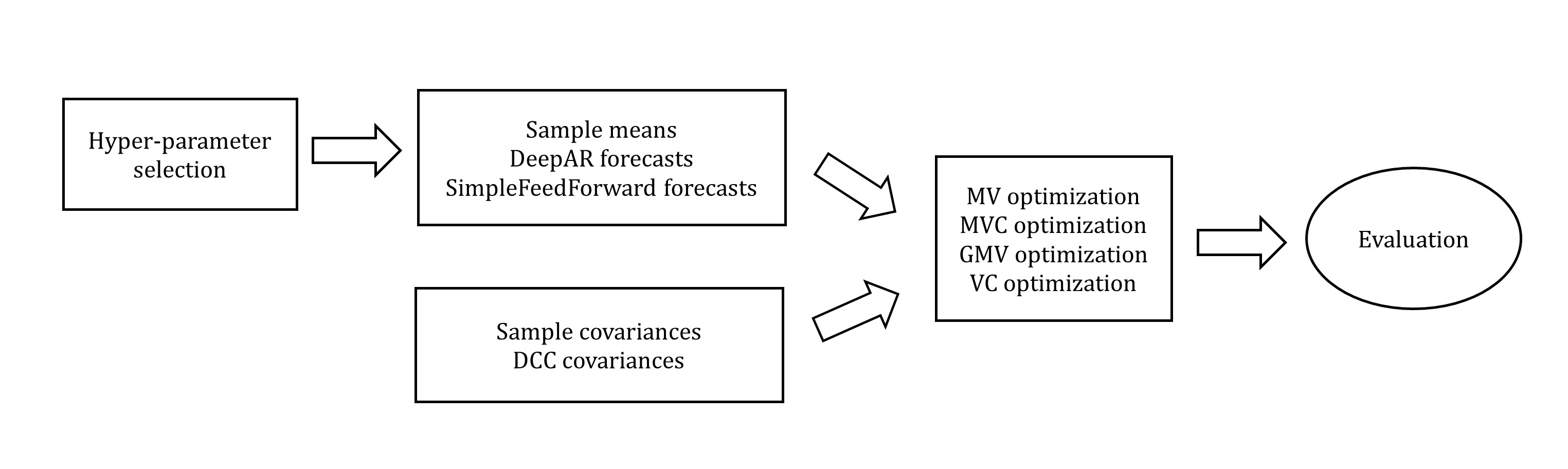
Figure 1: The entire pipeline for portfolio optimization and performance evaluation.

4.4 Evaluation

4.4.1 Performance fee

After the optimization process, we introduce the measure used in our study to evaluate the out-of-sample performance achieved by employed strategies. A widely used performance measure in mean-variance anlysis is the Sharpe ratio which is a risk-adjusted measure. However, according to Della Corte et al. (2009), several studies have suggested that the Share ratio severely underestimate the performance of a dynamic asset allocation strategy (Marquering and Verbeek (2004) and Han (2006)), owing to the overestimated conditional risk. Consequently, the evaluation criterion we adopt is the performance fee, which is computed by applying an extra fee to one of the selected strategy pair and then equating the two average realized utilities (Fleming et al., 2001). In this study, we compute the performance fees of various optimal portfolios relative to the naive 1/N rule. Following West et al. (1993), we assume a quadratic utility which justifies the mean-variance analysis with non-normal return distribution, consistent with our data. Subsequently, based on the work of Fleming et al. (2001), the performance fee $\Phi$ can be computed by solving the following equation:

$$\sum_{t=1}^{Q}{\{(R_{p,t}^{*}-\Phi)-\frac{\gamma}{2(1+\gamma)}(R_{p,t}^{*}-\Phi)^{2}\}}=\sum_{t=1}^{Q}{\{R_{p,t}-\frac{\gamma}{2(1+\gamma)}R_{p,t}^{2}\}},$$ (19)

where $R_{p,t}^{*}=1+r_{p,t}$ with $r_{p,t}$ denoting the realized portfolio return net of transaction costs achieved by optimal portfolio strategy, and $R_{p,t}=1+r_{p,t}^{n}$ with $r_{p,t}^{n}$ denoting the realized portfolio return net of transaction costs achieved by the 1/N rule, which is independent of risk aversion. The parameter $\gamma$ also represents the relative risk aversion, and we set it to be equal to the relative risk aversion coefficient by which $R_{p,t}^{*}$ is derived. The left side of equation 19 represents the utility achieved by the optimal strategy subjecting to a certain performance fee, and the right side represents the utility achieved by the benchmark strategy. An intuitive economic implication of performance fee is that it indicate the maximum fee an investor is willing pay to switch from the 1/N benchmark to the corresponding optimal portfolio strategy. Rearrange equation 19 by subtracting the right-hand side from the left-hand side, we have:

$$-\Phi^{2}+2(\frac{\sum_{t=1}^{Q}{R_{p,t}^{*}}}{Q}-\frac{1+\gamma}{\gamma})\Phi+2\frac{1+\gamma}{\gamma}\frac{\sum_{t=1}^{Q}{(R_{p,t}^{*}-R_{p,t})}}{Q}+\frac{\sum_{t=1}^{Q}{[R_{p,t}^{2}-(R_{p,t}^{*})^{2}]}}{Q}=0,$$ (20)

The left side of equation 20 represents the amount by which the utility achieved by the optimal strategy subjecting to performance fee exceeds that of the benchmark strategy, denoted by $\Delta U$. Solving this quadratic equation yields:

$$\Phi=\frac{B\pm\sqrt{B^{2}+4C}}{2},$$ (21)

where

$$B =2(\frac{\sum_{t=1}^{Q}{R_{p,t}^{*}}}{Q}-\frac{1+\gamma}{\gamma}),$$ (22)

$$C =2\frac{1+\gamma}{\gamma}\frac{\sum_{t=1}^{Q}{(R_{p,t}^{*}-R_{p,t})}}{Q}+\frac{\sum_{t=1}^{Q}{[R_{p,t}^{2}-(R_{p,t}^{*})^{2}]}}{Q}.$$ (23)

As shown in Figure 2, $\Delta U$ is greater than 0 in the interval $(\Phi_{1},\Phi_{2})$, where $\Phi_{1}=\frac{B-\sqrt{B^{2}+4C}}{2}$ and $\Phi_{2}=\frac{B+\sqrt{B^{2}+4C}}{2}$ are the two solutions of quadratic function. This means that an investor is willing pay a higher performance fee than $\Phi_{1}$ to switch from the 1/N benchmark to the corresponding optimal portfolio strategy, which contradicts the economic implication of performance fee. Hence, following Kirby and Ostdiek (2012), we discard the solution $\Phi_{1}$ and adopt the solution $\Phi_{2}$.

Figure 2: The amount by which the utility achieved by the optimal strategy subjecting to performance fee exceeds that of the benchmark strategy, $\Delta U$.

Further observing equation 21 $\sim$ equation 23, we find that we can achieve positive performance fee if $B>0$ and $B^{2}+4C\geq 0$. However, this is generally not the case, since $B$ is typically negative. Accordingly, the conditions $\frac{\sum_{t=1}^{Q}{R_{p,t}^{*}}}{Q}>\frac{\sum_{t=1}^{Q}{R_{p,t}}}{Q}$ and $\frac{\sum_{t=1}^{Q}{(R_{p,t}^{*})^{2}}}{Q}<\frac{\sum_{t=1}^{Q}{R_{p,t}^{2}}}{Q}$ facilitate genetating positive performance fee, which corresponds to a higher return and a lower risk than the benchmark strategy. Rearranging equation 20 once more, we have

$$-[\Phi-(\frac{\sum_{t=1}^{Q}{R_{p,t}^{*}}}{Q}-\frac{1+\gamma}{\gamma})]^{2}+D+\frac{\sum_{v\neq w}{2R_{p,v}^{*}R_{p,w}^{*}}}{Q^{2}}-\frac{(Q-1)\sum_{t=1}^{Q}{(R_{p,t}^{*})^{2}}}{Q^{2}}=0$$ (24)

where

$$D=(\frac{1+\gamma}{\gamma})^{2}-2\frac{1+\gamma}{\gamma}\frac{\sum_{t=1}^{Q}{R_{p,t}}}{Q}+\frac{\sum_{t=1}^{Q}{R_{p,t}^{2}}}{Q}$$ (25)

As shown in equation 24, given the performance of benchmark strategy, despite the existence of uncertain element ($\sum_{v\neq w}{2R_{p,v}^{*}R_{p,w}^{*}}$), however, increasing the return ($\sum_{t=1}^{Q}{R_{p,t}^{*}}/Q$) potentially shift the quadratic curve right and improve the resulting performance fee. Similarly, decreasing the risk ($\sum_{t=1}^{Q}{(R_{p,t}^{*})^{2}}/Q$) potentially shift the quadratic curve upward and also improve the resulting performance fee. Furthermore, since shifting right has a more direct effect than shifting upward on determining performance fee, the return play a more significant role than the risk.

4.4.2 Other metrics

We evaluate the performance of different portfolio strategies over the entire out-of-sample period. Since we derive an optimal portfolio across the risk aversion coefficient $\gamma$ from 1 to 10, we average these out-of-sample measures obtained using different values of $\gamma$. We first introduce the average annualized performance fee $\overline{PF}$ as follows:

$$\overline{PF}=\frac{1}{10}\sum_{\gamma=1}^{10}{\kappa\Phi_{2}^{\gamma}},$$ (26)

where $\kappa$ denotes a multiplier annualizing the performance fee and $\Phi_{2}^{\gamma}$ denotes the adopted performance fee solution achieved by using a particular $\gamma$.

In addition to the performance fee, we also employ other out-of-sample metrics to analyze the empirical results. Since the out-of-sample length is the same for all strategies, we directly compare the total out-of-sample portfolio return net of transaction costs. Similarly, we take an average across $\gamma$ from 1 to 10 and the average total out-of-sample portfolio return net of transaction costs $\overline{R_{p}}$ can be written as:

$$\overline{R_{p}}=\frac{1}{10}\sum_{\gamma=1}^{10}\sum_{t=1}^{Q}{R_{p,t}^{\gamma}},$$ (27)

where $R_{p,t}^{\gamma}$ denotes the portfolio return net of transaction costs achieved by using a particular $\gamma$ at time t.

We also care about the risk profile of portfolio and compute the average total out-of-sample portfolio risk $\overline{R_{p}^{2}}$ as follows:

$$\overline{R_{p}^{2}}=\frac{1}{10}\sum_{\gamma=1}^{10}\sum_{t=1}^{Q}{(R_{p,t}^{\gamma})^{2}},$$ (28)

To enhance empirical analysis, we further decompose the portfolio return net of transaction costs $\overline{R_{p}}$ into two components: the average total out-of-sample gross portfolio return $\overline{R_{g}}$ and the average total out-of-sample transaction costs $\overline{TC}$, and which can be written as:

$$\overline{R_{g}}=\frac{1}{10}\sum_{\gamma=1}^{10}\sum_{t=1}^{Q}{R_{g,t}^{\gamma}},$$ (29)

$$\overline{TC}=\frac{1}{10}\sum_{\gamma=1}^{10}\sum_{t=1}^{Q}{TC_{t}^{\gamma}},$$ (30)

where $R_{g,t}^{\gamma}$ and $TC_{t}^{\gamma}$ denote the gross portfolio return and the transaction cost achieved by using a particular $\gamma$ at time t respectively.

The forecasting accuracy is evaluated by the aggregate RMSE measure as defined above, but replace the validation set with the test set. Furthermore, we examine the variation characteristic of different conditional moment estimators. The $L_{2}$-norm and the Frobenius norm are employed to measure the variation levels ($VL$) of different return forecasting series and estimated covariance matrices respectively, which can be represented as:

$$VL_{mean}=\frac{\sum_{t=1}^{Q-1}{||\hat{r}_{t+1}-\hat{r}_{t}||_{2}}}{Q-1}=\frac{\sum_{t=1}^{Q-1}{\sqrt{\sum_{i=1}^{N}{(\hat{r}_{i,t+1}-\hat{r}_{i,t})^{2}}}}}{Q-1},$$ (31)

$$VL_{cov}=\frac{\sum_{t=1}^{Q-1}{||\hat{\Sigma}_{t+1}-\hat{\Sigma}_{t}||_{F}}}{Q-1}=\frac{\sum_{t=1}^{Q-1}{\sqrt{\sum_{i,j}{(\hat{\Sigma}_{ij,t+1}-\hat{\Sigma}_{ij,t})^{2}}}}}{Q-1}.$$ (32)

Table 4: The one-step-ahead forecasting accuracy and the variation levels.

Panel A: The forecasting accuracy.
	SM	DA	SFF	sample cov	DCC cov
daily case	0.0477	0.0479	0.0480	–	–
weekly case	0.1252	0.1296	0.1292	–	–

Panel B: The variation levels.
	SM	DA	SFF	sample cov	DCC cov
daily case	0.0006	0.0162	0.0148	0.0001	0.0054
weekly case	0.0113	0.1152	0.0088	0.0038	0.0370

Note: “SM”, “DA”, and “SFF” indicate the sample means, DeepAR forecasts, and SimpleFeedForward forecasts, respectively.

5 Empirical results and discussion

This section reports and discusses the empirical results for daily and weekly rebalancing cases. On a risk-adjusted basis, the portfolio performance is determined by risk and return. We further decompose the return net of transaction costs $\overline{R_{p}}$ into the gross return $\overline{R_{g}}$ and the transaction costs $\overline{TC}$. Accordingly, we systematically analyze how different methods affect the three aspects (the gross return $\overline{R_{g}}$, the transaction costs $\overline{TC}$ and the portfolio risk $\overline{R_{p}^{2}}$) that determine portfolio performance.

In detail, regarding $\overline{R_{g}}$, we believe that the conditional mean estimates are associated with the term $w_{t}^{\prime}\mu_{t+1|t}$, and accurate return forecasts should lead to desired gross return measure. For the risk $\overline{R_{p}^{2}}$, the conditional covariance estimates are associated with the term $w_{t}^{\prime}\Sigma_{t+1|t}w_{t}$, and accurate volatility forecasts should reduce the portfolio risk. In addition, a high variation level of estimator also tends to increase the portfolio volatility. Finally, with respect to the transaction costs $\overline{TC}$, the turnover penalty term $\beta||w_{t}-w_{t-1^{+}}^{*}||_{1}$ can inhibit excessive rebalancing and a high variation level of estimator also incurs considerable transaction fees.

Table 5: The average total out-of-sample portfolio returns net of transaction costs $\overline{R_{p}}$, average total out-of-sample portfolio risk $\overline{R_{p}^{2}}$, average total out-of-sample gross portfolio returns $\overline{R_{g}}$ and average total out-of-sample transaction costs $\overline{TC}$ achieved by the MV optimization framework, for daily and weekly rebalancing cases.

Panel A: Average total out-of-sample portfolio returns net of transaction costs $\overline{R_{p}}$.
	1/N	SM	DA	SFF
daily case	-0.2004	-0.8756	-5.0248	-4.9959
weekly case	-0.3538	-0.8419	-1.9713	-0.5182

Panel B: Average total out-of-sample portfolio risk $\overline{R_{p}^{2}}$.
	1/N	SM	DA	SFF
daily case	1.5291	1.2912	1.9159	1.7309
weekly case	1.4165	1.3784	1.4663	1.3201

Panel C: Average total out-of-sample gross portfolio returns $\overline{R_{g}}$.
	1/N	SM	DA	SFF
daily case	-0.1354	-0.6103	0.5019	0.0358
weekly case	-0.3238	-0.7056	-1.1329	-0.3073

Panel D: Average total out-of-sample transaction costs $\overline{TC}$.
	1/N	SM	DA	SFF
daily case	0.0651	0.2653	5.5267	5.0316
weekly case	0.0300	0.1363	0.8384	0.2108

5.1 The results of the MV optimization framework

We begin with examining the characteristics of return forecasting series obtained from different methods. The first one is the forecasting accuracy evaluated by the aggregate RMSE measure. As shown in Panel A of Table 4, the forecasting accuracy of all methods is similar, suggesting that it is not the primary cause of the performance differences in optimal portfolios. These forecasting accuracy values (aggregate RMSE) correspond to a daily prediction error of nearly 5% and a weekly prediction error of 12% $\sim$ 13%, which suggest considerable errors and that the mean predictive models considered in this study have essentially no predictive ability. Accordingly, although the gross returns $\overline{R_{g}}$ vary across optimal strategies as shown in Panel C of Table 5, we understand this as an outcome of specific data. On the other hand, half of the optimal strategies produce markedly worse gross return values $\overline{R_{g}}$ than those achieved by the naive 1/N benchmark, which we attribute to the considerable forecasting errors.

Subsequently, we further examine the variation characteristic of different return forecasting series and Panel B of Table 4 shows that the variation levels of deep learning forecasting series are substantially higher than those of the sample mean series. One exception is the weekly SimpleFeedForward forecasts which calculate the average of 1000 sample paths, and the SimpleFeedForward model is a relatively simple deep learning model. A high variation level can lead to frequent rebalancing as well as large transaction fees, as can be seen from Panel D in Table 5, deep learning forecasts require obviously larger transaction costs than simple means, except for weekly SimpleFeedForward forecasts.

For daily rebalancing case, if an optimal portfolio strategy adopts deep learning forecasts and doesn’t impose the turnover penalty, then the portfolio performance primarily depends on the transaction costs incurred by deep learning forecasts rather than the impact of gross return $\overline{R_{g}}$. For example, the MV optimal strategy using DeepAR forecasts achieves the highest gross return 0.5019, which is substantially less crucial compared to the required transaction costs 5.5267.

Interestingly, as the most stable return estimates, weekly SimpleFeedForward forecasts produce a slightly larger $\overline{TC}$ value than simple means. One possible explanation is that weekly SimpleFeedForward forecasts are overly stable and the transaction costs are dominated by the variation level of simple covariances. However, the variation levels of sample means and simple covariances are comparable and their effects may cancel out each other, resulting in lower turnover. We refer to this phenomenon as the “offset effect” hereafter (this effect is more obvious when employing DCC covariances and we will enhance this claim in robust test).

Accordingly, all optimal strategies produce poor and sometimes even unreasonable portfolio return net of transaction costs $\overline{R_{p}}$ values as indicated in Panel A of Table 5. On the other hand, another determining factor of performance fee, the portfolio risk $\overline{R_{p}^{2}}$ values vary across optimal strategies. Specifically, daily deep learning forecasts obviously increase portfolio risk, due to their high variation levels. However, the annualized performance fee $\overline{PF}$ values as reported in Table 6 seems to primarily follow corresponding $\overline{R_{p}}$ values, which justifies our previous claim that return plays a more significant role than risk in determining performance fee.

Table 6: The average annualized performance fees $\overline{PF}$ achieved by the MV optimization framework, for daily and weekly rebalancing cases.

	Panel A: daily case			Panel B: weekly case
	SM	DA	SFF	SM	DA	SFF
$\overline{PF}$	-0.2387	-2.0798	-2.0319	-0.1931	-0.6749	-0.0459

Note: “SM”, “DA”, and “SFF” indicate the sample means, DeepAR forecasts, and SimpleFeedForward forecasts, respectively.

Table 7: The average total out-of-sample portfolio returns net of transaction costs $\overline{R_{p}}$, average total out-of-sample portfolio risk $\overline{R_{p}^{2}}$, average total out-of-sample gross portfolio returns $\overline{R_{g}}$ and average total out-of-sample transaction costs $\overline{TC}$ achieved by the GMV optimization framework, for daily and weekly rebalancing cases.

Panel A: Average total out-of-sample portfolio returns net of transaction costs $\overline{R_{p}}$.
	1/N	sample cov	DCC cov
daily case	-0.2004	-0.2163	-0.7593
weekly case	-0.3538	-0.1389	-0.2706

Panel B: Average total out-of-sample portfolio risk $\overline{R_{p}^{2}}$.
	1/N	sample cov	DCC cov
daily case	1.5291	1.0512	1.0930
weekly case	1.4165	1.2205	1.2240

Panel C: Average total out-of-sample gross portfolio returns $\overline{R_{g}}$.
	1/N	sample cov	DCC cov
daily case	-0.1354	-0.1730	-0.1344
weekly case	-0.3238	-0.0602	-0.1174

Panel D: Average total out-of-sample transaction costs $\overline{TC}$.
	1/N	sample cov	DCC cov
daily case	0.0651	0.0433	0.6249
weekly case	0.0300	0.0787	0.1533

5.2 The results of the GMV optimization framework

As indicated above, all the MV optimal strategies produce negative performance fees (i.e. underperformed by the naive 1/N benchmark). That is to say, the gains from optimal allocation are not sufficient to compensate the side effect of estimation error for all the MV portfolios. In the analysis above, we attribute the poor performance of optimal strategies largely to the variation characteristic of estimates. However, we calculate the actual variation levels of the test set data to be 0.1067 for daily returns and 0.2956 for weekly returns, which are even substantially greater than those of deep learning forecasts. Actually, the variation levels of deep learning forecasts are closer to the actual ones, but due to the lack of prediction ability for the conditional means, frequent rebalancing has brought no gains, but only large transaction fees.

We then turn to the GMV optimization framework without utilizing the conditional mean estimates. According to Table 7 and Table 8, it is evident that the GMV optimization combined with sample covariances outperforms its counterpart utilizing return estimates, regardless of daily or weekly case. This suggests that utilizing return estimates is not beneficial to improving portfolio performance and justifies the exclusion of mean estimates by that the input which cannot be estimated accurately should be discarded.

In detail, from Panel B of Table 7, we notice that the volatility time strategies obviously improvement the risk values $\overline{R_{p}^{2}}$ for all portfolios. Moreover, simple covariances achieve slightly better risk improvement results, which might be due to the high variation levels of DCC covariances.

Subsequently, we examine the impact of covariance estimates on $\overline{R_{g}}$ and $\overline{TC}$, which determine $\overline{R_{p}}$. Firstly, the volatility timing strategies don’t involve return forecasting, and thus we understand the varying $\overline{R_{g}}$ results as an outcome of specific data. Regarding the transaction costs, as shown in Panel D of Table 7, it is evident that DCC covariances require larger $\overline{TC}$ values, especially for daily case.

Consequently, daily DCC covariances lead to poor performance like previous deep learning forecasts, which suggest that the gains from the frequent rebalancing caused by DCC covariances also cannot offset the transaction costs incurred. Meanwhile, other volatility timing strategies all produce positive performance fees, as indicated in Table 8. Although in volatility timing strategies, the performance fees still principally follow the return $\overline{R_{p}}$, which further enhances our previous analytic claim.

Table 8: The average annualized performance fees $\overline{PF}$ achieved by the GMV optimization framework, for daily and weekly rebalancing cases.

	Panel A: daily case		Panel B: weekly case
	sample cov	DCC cov	sample cov	DCC cov
$\overline{PF}$	0.0733	-0.1614	0.1217	0.0664

Table 9: The average total out-of-sample portfolio returns net of transaction costs $\overline{R_{p}}$, average total out-of-sample portfolio risk $\overline{R_{p}^{2}}$, average total out-of-sample gross portfolio returns $\overline{R_{g}}$ and average total out-of-sample transaction costs $\overline{TC}$ achieved by the MVC and the VC optimization frameworks, for daily and weekly rebalancing cases.

Panel A: Average total out-of-sample portfolio returns net of transaction costs $\overline{R_{p}}$.
	1/N	SM	DA	SFF	sample cov	DCC cov
daily case	-0.2004	-0.4812	-1.9421	-0.3437	-0.4607	-0.0024
weekly case	-0.3538	-0.6632	-1.5216	-0.4742	-0.3511	-0.2157

Panel B: Average total out-of-sample portfolio risk $\overline{R_{p}^{2}}$.
	1/N	SM	DA	SFF	sample cov	DCC cov
daily case	1.5291	1.0292	1.4435	1.2213	1.0616	1.2061
weekly case	1.4165	1.3357	1.5649	1.2299	1.1484	1.2698

Panel C: Average total out-of-sample gross portfolio returns $\overline{R_{g}}$.
	1/N	SM	DA	SFF	sample cov	DCC cov
daily case	-0.1354	-0.4761	-0.6647	-0.1785	-0.4556	0.0254
weekly case	-0.3238	-0.6170	-0.7937	-0.4548	-0.3367	-0.1444

Panel D: Average total out-of-sample transaction costs $\overline{TC}$.
	1/N	SM	DA	SFF	sample cov	DCC cov
daily case	0.0651	0.0050	1.2774	0.1652	0.0051	0.0278
weekly case	0.0300	0.0463	0.7279	0.0194	0.0144	0.0714

5.3 The results with turnover penalty

We next examine the empirical results of previous two optimization frameworks with imposing turnover penalty, namely the MVC and the VC optimization framework. Comparing Panel D of Table 9 with that of Table 5 and Table 7, it is evident that the turnover penalty obviously reduces the transaction costs $\overline{TC}$ required for all optimal portfolios. This improvement is particularly marked for high-frequency strategies and highly volatile moment estimates.

Regarding the gross returns $R_{g}$, comparing Panel C of Table 9 with that of Table 5 and Table 7, it appears that the turnover penalty plays neither a good nor a bad role. This seems to suggest that our forecasting models just have no predictive power, but haven’t yet produced the opposite prediction.

Similarly, comparing Panel B of Table 9 with that of Table 5 and Table 7, we find that the turnover penalty tends to reduce the risk $\overline{R_{p}^{2}}$ of the MV optimal strategies, since it inhibits excessive rebalancing which may increase volatility. Nevertheless, for the GMV optimal strategies, the turnover penalty tends to increase the risk $\overline{R_{p}^{2}}$, suggesting it may inhibit the volatility timing strategies minimize the volatility.

However, the impact of risk $\overline{R_{p}^{2}}$ is slight, as a result, the performance fees primarily follow the return values $\overline{R_{p}}$. Comparing Table 10 with Table 6 and Table 8, we find that imposing turnover penalty substantially improves the portfolio performance in terms of performance fee for all MV optimal portfolios, which justifies the significance of turnover penalty in mean-variance analysis. However, in volatility timing strategies, the turnover penalty only improves the performance of DCC covariances but not sample estimates. The explanation is intuitive that stable sample covariances require only little transaction fees and thus the benefits of turnover penalty are not crucial.

Furthermore, it seems that the improvement resulting from the turnover penalty becomes less noticeable for lower rebalancing frequency. This is consistent with our previous analytic claim that the lower the rebalancing frequency, the smaller the change caused by the turnover penalty will be.

What’s more, although in presence of interaction, previous conclusions can generally be re-examined in the empirical results after imposing turnover penalty, such as the impact of variation levels, the improvement on portfolio risk, the role of returns $\overline{R_{p}}$ in determining performance fees, etc.

5.4 Summary

Whether imposing the turnover penalty or not, the volatility timing strategies and the naive 1/N benchmark both outperform the optimization frameworks utilizing return estimates, which suggests that it’s difficult for us to exploit the possible predictability of asset returns. On the other hand, even in highly correlated cryptocurrency market, the volatility timing portfolios can also slightly outperform the naive 1/N benchmark, which justifies the economic value of predictability of asset return volatility. Better performance may be achieved in other more idiosyncratic market or diversified portfolio. The improvement relative to the naive 1/N strategy is slight, which is partly attributed to the highly correlated market and also suggests that the gains from optimal allocation will not be significant if we rely solely on daily or weekly historical data.

Table 10: The average annualized performance fees $\overline{PF}$ achieved by the MVC and the VC optimization frameworks, for daily and weekly rebalancing cases.

	SM	DA	SFF	sample cov	DCC cov
daily case	-0.0343	-0.7114	-0.0043	-0.0309	0.1395
weekly case	-0.1114	-0.5055	-0.0143	0.0456	0.0829

Note: “SM”, “DA”, and “SFF” indicate the sample means, DeepAR forecasts, and SimpleFeedForward forecasts, respectively.

6 Conclusion

In this study, we consider several alternative methods for portfolio optimization. Subsequently, we detail how these methods affect the three aspects that determine portfolio performance (the portfolio risk $\overline{R_{p}^{2}}$, the gross return $\overline{R_{g}}$ and the transaction costs $\overline{TC}$). Meanwhile, we emphasize the role of estimates’ variation levels. With respect to the performance evaluation, we employ the performance fee to measure the economic value. A higher return $\overline{R_{p}}$ and lower risk $\overline{R_{p}^{2}}$ lead to a better performance fee result, and the return plays a more significant role than the risk. Our main findings are as follows:

(I) Depending solely on historical data (deep learning models train parameters using a “cross-learning” approach), deep learning models cannot produce more accurate forecasts than sample means and the errors are even slightly larger, which is similar to the results of Makridakis et al. (2023). However, on the other hand, the predictability of asset return volatility obviously improves portfolio risk, regardless of in the volatility timing or mean-variance context.

(II) We find that the estimators obtained from sophisticated methods (deep learning forecasts, DCC covariances) tend to be more volatile than their sample counterparts and usually lead to poor performance. Since the performance of moment estimation relies not only on the forecasting accuracy, but also on the variation level, especially for conditional mean estimation. With similar forecasting accuracy, the one with lower variation level is preferred. A higher variation level tends to result in larger transaction costs and higher portfolio risk, which deteriorate portfolio performance. Our finding coincides with and enhances the discussions in Fleming et al. (2001), Fleming et al. (2003), Kirby and Ostdiek (2012) and Kynigakis and Panopoulou (2022).

(III) The empirical results justify the significance of turnover penalty in reducing transaction costs and improving performance under a mean-variance context, which is consistent with Yoshimoto (1996) and Olivares-Nadal and DeMiguel (2018). For volatility timing strategies, the portfolios using DCC covariances are obviously improved and achieve comparable performance to those using sample estimates, which extends the finding in Fleming et al. (2001) and Fleming et al. (2003). Nevertheless, our turnover penalty ($L_{1}$-norm) isn’t beneficial for the portfolios using sample covariances, which effectively corresponds to the results of shortsale-constrained minimum-variance portfolio with nominal transaction costs in Olivares-Nadal and DeMiguel (2018). Furthermore, our analytical derivation suggests that the improvement resulting from turnover penalty will diminish as the rebalancing frequency decreases, which is similar to Woodside-Oriakhi et al. (2013), and our empirical results also confirm this.

(IV) Even in highly correlated cryptocurrency market, most of the volatility timing portfolios achieve positive performance fees and obviously outperform their counterparts depending on return estimates, which justifies the economic value of predictability of asset return volatility. Even after the turnover penalty is imposed, the portfolios utilizing return estimates are also inferior to those volatility timing portfolios and the naive 1/N benchmark, which reconfirms that it’s difficult to capture the possible predictability of asset return in order to produce investment gains.

Appendix

Appendix A: Proof of Proposition 1

Proof.

Let $w_{t}^{MVC,*}$ be the solution of the MVC optimization problem, then it should satisfy the first-order conditions:

$$\gamma\Sigma_{t|t+1}w_{t}^{MVC,*}+\beta g^{*}-\mu_{t|t+1}-\lambda l =0,$$ (33)

$$l^{\prime}w_{t}^{MVC,*}-1 =0,$$ (34)

where $g^{*}$ is the subgradient vector of function $||w_{t}-w_{t-1^{+}}^{*}||_{1}$ evaluated at $w_{t}^{*}$ and $\lambda$ is the Lagrange multiplier. Solving for $w_{t}^{MVC,*}$ yields,

$$w_{t}^{MVC,*}=\frac{1}{\gamma}(\Sigma_{t|t+1}^{-1}-\frac{\Sigma_{t|t+1}^{-1}ll^{\prime}\Sigma_{t|t+1}^{-1}}{l^{\prime}\Sigma_{t|t+1}^{-1}l})(\mu_{t|t+1}-\beta g^{*})+\frac{\Sigma_{t|t+1}^{-1}l}{l^{\prime}\Sigma_{t|t+1}^{-1}l},$$ (35)

Let $\tilde{w}_{t}^{*}$ be the solution of the MV optimization problem with the mean estimator $\tilde{\mu}_{t|t+1}=\mu_{t|t+1}-\beta g^{*}$, by using the classical efficient portfolio representation, we have

$$\tilde{w}_{t}^{*} =\frac{1}{\gamma}(\Sigma_{t|t+1}^{-1}-\frac{\Sigma_{t|t+1}^{-1}ll^{\prime}\Sigma_{t|t+1}^{-1}}{l^{\prime}\Sigma_{t|t+1}^{-1}l})\tilde{\mu}_{t|t+1}+\frac{\Sigma_{t|t+1}^{-1}l}{l^{\prime}\Sigma_{t|t+1}^{-1}l}$$ (36)

$$=\frac{1}{\gamma}(\Sigma_{t|t+1}^{-1}-\frac{\Sigma_{t|t+1}^{-1}ll^{\prime}\Sigma_{t|t+1}^{-1}}{l^{\prime}\Sigma_{t|t+1}^{-1}l})(\mu_{t|t+1}-\beta g^{*})+\frac{\Sigma_{t|t+1}^{-1}l}{l^{\prime}\Sigma_{t|t+1}^{-1}l}.$$ (37)

Consequently, $w_{t}^{MVC,*}=\tilde{w}_{t}^{*}$, and the Proposition 1 holds. ∎

Appendix B: Implementation details for hyper-parameter selection

For the DeepAR model, we consider seven hyper-parameters: “num_layers” which represents the number of RNN layers; “hidden_size” which represents the number of RNN cells for each layer; “batch_size” which represents the size of the batches used for training; “max_epochs” which is a part of the hyper-parameter “trainer_kwargs” and represents an additional argument to provide to pl.Trainer for construction; “num_batches_per_epoch” which represents the number of batches to be processed in each training epoch; “lr” which defines the learning rate; and “num_samples” which is the number of samples to draw on the model. Six of these hyper-parameters are defined as categorical hyper-parameters, with respective search spaces listed as $[1,2,3]$ for “num_layers”, $[2,4,8,16]$ for “hidden_size”, $[2,4,8,16]$ for “batch_size”, $[8,16,32,64,128]$ for “max_epochs”, $[2,4,8,16]$ for “num_batches_per_epoch”, and $[10,100,1000]$ for “num_samples”. While “lr” is defined as floating point (log) hyper-parameter and ranges between $5e^{-4}$ and $5e^{-3}$.

In regard to the SimpleFeedForward model, we take into account six important hyper-parameters: “batch_size”, “max_epochs”, “num_batches_per_epoch”, “lr” and “num_samples” which are similar to those in the DeepAR model; “hidden_dimensions” which represents the size of hidden layers in the feed-forward network. The explanations of hyper-parameters are obtained from https://ts.gluon.ai/stable/index.html. We consider the search spaces $[4,8,16,32]$ for “batch_size”, $[16,32,64,128,256]$ for “max_epochs”, $[4,8,16,32]$ for “num_batches_per_epoch”, and $[10,100,1000]$ for “num_samples”, while the floating point (log) hyper-parameter “lr” ranges between $5e^{-4}$ and $5e^{-3}$ and a series of indicative sizes are considered for “hidden_dimensions”. The selected hyper-parameter values are reported in Table A1 and Table A2.

Table A1: The selected hyper-parameter values for the DeepAR model for daily and weekly data.

	daily	weekly
num_layers	1	1
hidden_size	8	16
batch_size	16	2
max_epochs	64	16
num_batches_per_epoch	4	2
lr	0.0022	0.0036
num_samples	100	10

Table A2: The selected hyper-parameter values for the SimpleFeedForward model for daily and weekly data.

	daily	weekly
hidden_dimensions	[16]	[2, 2]
batch_size	8	32
max_epochs	128	32
num_batches_per_epoch	4	4
lr	0.0037	0.0016
num_samples	100	1000

References

- Ackermann et al. [2017] F. Ackermann, W. Pohl, and K. Schmedders. Optimal and naive diversification in currency markets. Management Science, 63(10):3347–3360, 2017.
- Ahmed et al. [2016] S. Ahmed, X. Liu, and G. Valente. Can currency-based risk factors help forecast exchange rates? International Journal of Forecasting, 32(1):75–97, 2016.
- Alexandrov et al. [2019] A. Alexandrov, K. Benidis, M. Bohlke-Schneider, V. Flunkert, J. Gasthaus, T. Januschowski, D. C. Maddix, S. Rangapuram, D. Salinas, J. Schulz, et al. Gluonts: Probabilistic time series models in python. arXiv preprint arXiv:1906.05264, 2019.
- Bergstra et al. [2011] J. Bergstra, R. Bardenet, Y. Bengio, and B. Kégl. Algorithms for hyper-parameter optimization. Advances in neural information processing systems, 24, 2011.
- Cheikh et al. [2020] N. B. Cheikh, Y. B. Zaied, and J. Chevallier. Asymmetric volatility in cryptocurrency markets: New evidence from smooth transition garch models. Finance Research Letters, 35:101293, 2020.
- Chen et al. [2021] W. Chen, H. Zhang, M. K. Mehlawat, and L. Jia. Mean–variance portfolio optimization using machine learning-based stock price prediction. Applied Soft Computing, 100:106943, 2021.
- Chopra and Ziemba [1993] V. K. Chopra and W. T. Ziemba. The effect of errors in means, variances, and covariances on optimal portfolio choice. The Journal of Portfolio Management, 19(2):6–11, 1993.
- Christoffersen et al. [2014] P. Christoffersen, V. Errunza, K. Jacobs, and X. Jin. Correlation dynamics and international diversification benefits. International Journal of Forecasting, 30(3):807–824, 2014.
- Della Corte et al. [2009] P. Della Corte, L. Sarno, and I. Tsiakas. An economic evaluation of empirical exchange rate models. The review of financial studies, 22(9):3491–3530, 2009.
- DeMiguel et al. [2009] V. DeMiguel, L. Garlappi, and R. Uppal. Optimal versus naive diversification: How inefficient is the 1/n portfolio strategy? The review of Financial studies, 22(5):1915–1953, 2009.
- Du [2022] J. Du. Mean–variance portfolio optimization with deep learning based-forecasts for cointegrated stocks. Expert Systems with Applications, 201:117005, 2022.
- D’Hondt et al. [2020] C. D’Hondt, R. De Winne, E. Ghysels, and S. Raymond. Artificial intelligence alter egos: Who might benefit from robo-investing? Journal of Empirical Finance, 59:278–299, 2020.
- Engle [2002] R. Engle. Dynamic conditional correlation: A simple class of multivariate generalized autoregressive conditional heteroskedasticity models. Journal of Business & Economic Statistics, 20(3):339–350, 2002.
- Fleming et al. [2001] J. Fleming, C. Kirby, and B. Ostdiek. The economic value of volatility timing. The Journal of Finance, 56(1):329–352, 2001.
- Fleming et al. [2003] J. Fleming, C. Kirby, and B. Ostdiek. The economic value of volatility timing using “realized” volatility. Journal of Financial Economics, 67(3):473–509, 2003.
- Gao and Nardari [2018] X. Gao and F. Nardari. Do commodities add economic value in asset allocation? new evidence from time-varying moments. Journal of Financial and Quantitative Analysis, 53(1):365–393, 2018.
- Golnari et al. [2024] A. Golnari, M. H. Komeili, and Z. Azizi. Probabilistic deep learning and transfer learning for robust cryptocurrency price prediction. Expert Systems with Applications, page 124404, 2024.
- Han [2006] Y. Han. Asset allocation with a high dimensional latent factor stochastic volatility model. The Review of Financial Studies, 19(1):237–271, 2006.
- Hautsch and Voigt [2019] N. Hautsch and S. Voigt. Large-scale portfolio allocation under transaction costs and model uncertainty. Journal of Econometrics, 212(1):221–240, 2019.
- Januschowski et al. [2020] T. Januschowski, J. Gasthaus, Y. Wang, D. Salinas, V. Flunkert, M. Bohlke-Schneider, and L. Callot. Criteria for classifying forecasting methods. International Journal of Forecasting, 36(1):167–177, 2020.
- Kan and Zhou [2007] R. Kan and G. Zhou. Optimal portfolio choice with parameter uncertainty. Journal of Financial and Quantitative Analysis, 42(3):621–656, 2007.
- Katsiampa et al. [2019] P. Katsiampa, S. Corbet, and B. Lucey. High frequency volatility co-movements in cryptocurrency markets. Journal of International Financial Markets, Institutions and Money, 62:35–52, 2019.
- Kirby and Ostdiek [2012] C. Kirby and B. Ostdiek. It’s all in the timing: simple active portfolio strategies that outperform naive diversification. Journal of financial and quantitative analysis, 47(2):437–467, 2012.
- Kynigakis and Panopoulou [2022] I. Kynigakis and E. Panopoulou. Does model complexity add value to asset allocation? evidence from machine learning forecasting models. Journal of Applied Econometrics, 37(3):603–639, 2022.
- Li et al. [2024] J. Li, W. Chen, Z. Zhou, J. Yang, and D. Zeng. Deepar-attention probabilistic prediction for stock price series. Neural Computing and Applications, pages 1–18, 2024.
- Ma et al. [2021] Y. Ma, R. Han, and W. Wang. Portfolio optimization with return prediction using deep learning and machine learning. Expert Systems with Applications, 165:113973, 2021.
- Makridakis et al. [2023] S. Makridakis, E. Spiliotis, V. Assimakopoulos, A.-A. Semenoglou, G. Mulder, and K. Nikolopoulos. Statistical, machine learning and deep learning forecasting methods: Comparisons and ways forward. Journal of the Operational Research Society, 74(3):840–859, 2023.
- Marquering and Verbeek [2004] W. Marquering and M. Verbeek. The economic value of predicting stock index returns and volatility. Journal of Financial and Quantitative Analysis, 39(2):407–429, 2004.
- Michaud [1989] R. O. Michaud. The markowitz optimization enigma: Is ‘optimized’optimal? Financial analysts journal, 45(1):31–42, 1989.
- Nelson [1991] D. B. Nelson. Conditional heteroskedasticity in asset returns: A new approach. Econometrica: Journal of the econometric society, pages 347–370, 1991.
- Olivares-Nadal and DeMiguel [2018] A. V. Olivares-Nadal and V. DeMiguel. A robust perspective on transaction costs in portfolio optimization. Operations Research, 66(3):733–739, 2018.
- Opie and Riddiough [2020] W. Opie and S. J. Riddiough. Global currency hedging with common risk factors. Journal of Financial Economics, 136(3):780–805, 2020.
- Platanakis et al. [2018] E. Platanakis, C. Sutcliffe, and A. Urquhart. Optimal vs naïve diversification in cryptocurrencies. Economics Letters, 171:93–96, 2018.
- Salinas et al. [2020] D. Salinas, V. Flunkert, J. Gasthaus, and T. Januschowski. Deepar: Probabilistic forecasting with autoregressive recurrent networks. International Journal of Forecasting, 36(3):1181–1191, 2020.
- Tu and Zhou [2011] J. Tu and G. Zhou. Markowitz meets talmud: A combination of sophisticated and naive diversification strategies. Journal of Financial Economics, 99(1):204–215, 2011.
- West et al. [1993] K. D. West, H. J. Edison, and D. Cho. A utility-based comparison of some models of exchange rate volatility. Journal of international economics, 35(1-2):23–45, 1993.
- Woodside-Oriakhi et al. [2013] M. Woodside-Oriakhi, C. Lucas, and J. E. Beasley. Portfolio rebalancing with an investment horizon and transaction costs. Omega, 41(2):406–420, 2013.
- Yoshimoto [1996] A. Yoshimoto. The mean-variance approach to portfolio optimization subject to transaction costs. Journal of the Operations Research Society of Japan, 39(1):99–117, 1996.