Weighted Point Configurations
with Hyperuniformity:
An Ecological Example and Models

Abstract

Random point configurations are said to be in hyperuniform states, if density fluctuations are anomalously suppressed in large-scale. Typical examples are found in Coulomb gas systems in two dimensions especially called log-gases in random matrix theory, in which points are repulsively correlated by long-range potentials. In infertile lands like deserts continuous survival competitions for water and nutrition will cause long-ranged repulsive interactions among plants. We have prepared digital data of spatial configurations of center-of-mass for bushes weighted by bush sizes which we call masses. Data analysis shows that such ecological point configurations do not show hyperuniformity as unmarked point processes, but are in hyperuniform states as marked point processes in which mass distributions are taken into account. We propose the non-equilibrium statistical-mechanics models to generate marked point processes having hyperuniformity, in which iterations of random thinning of points and coalescing of masses transform initial uncorrelated point processes into non-trivial point processes with hyperuniformity. Combination of real data-analysis and computer simulations shows the importance of strong correlations in probability law between spatial point configurations and mass distributions of individual points to realize hyperuniform marked point processes.

1 Introduction

Structures and distribution of ordered and disordered configurations of points in a space have been important research subjects in physics, where the points represent the locations of atoms or molecules in gases, liquids, glasses, and crystals. If we consider a classical ideal-gas, the spatial configurations of molecules are completely random and the statistical ensembles of such uncorrelated point configurations is identified with the Poisson point process (PPP) studied in mathematics [2, 5]. In mathematical physics and probability theory spatial statistics of (random) configurations of points are simply called a (random) point process in general [2, 5]. Correlated point processes have been also extensively studied in statistical mechanics for Coulomb gas systems, which are especially called the log-gases in one- and two-dimensional spaces [6]. It is known that they are are realized as the eigenvalue distributions of Hermitian and non-Hermitian random matrices [4, 6, 7, 10, 19] and as the zeros of random analytic functions [9, 13].

Recently in condensed matter physics and related material sciences, correlated particle systems are said to be in a hyperuniform state, when density fluctuations are anomalously suppressed in large-scale [33]. Consider a bounded domain with linear size $\ell$ in the $d$-dimensional space, which we call an observation window. In this window we measure the mean number of points $\langle N_{\ell}\rangle$ and its variance $\sigma^{2}_{\ell}$. In a hyperuniform system, as the window size $\ell\to\infty$, $\sigma^{2}_{\ell}$ grows more slowly than $\langle N_{\ell}\rangle$ which is proportional to the window volume. Typical disordered systems (e.g., liquids and structured glasses) have the standard scaling behavior $\sigma_{\ell}\sim\ell^{d}$ as $\ell\to\infty$, and hence they are not hyperuniform. Periodic point configuration (e.g., lattice points of crystals) are obviously hyperuniform systems, since the number fluctuations are concentrated near the window boundary and hence have the surface-area scaling $\sigma^{2}_{\ell}\sim\ell^{d-1}$ as $\ell\to\infty$. We are interested in the hyperuniform point processes, which are not perfect lattice, but are randomly distributed following some probability laws. A variety of examples of disordered or random point processes showing hyperuniformity have been reported in the review paper by Torquato [33]. A typical example on the two-dimensional plane, which has been well studied in mathematical physics, is the complex Ginibre point process (GPP) [7]. This is realized as the statistical ensemble of eigenvalues of non-Hermitian random matrices on the complex plane $\mathbb{C}$, which can be identified with the two-dimensional space $\mathbb{R}^{2}$. There first we consider an $n\times n$ matrix whose entries are all independently and identically distributed (i.i.d.) complex standard Gaussian random variables. We have a nearly uniform distribution of eigenvalues in a disk centered at the origin with radius proportional to $\sqrt{n}$ on $\mathbb{C}$. If we consider the $n\to\infty$ limit, we have a translation-invariant point process on $\mathbb{C}$ [7]. It was proved that the obtained GPP is hyperuniform with $\sigma_{\ell}\sim\ell$ [26]. The origin of such hyperuniformity in random point configuration is long-ranged repulsive interaction between any pair of points. As a matter of fact, GPP is a determinantal point process (DPP) [9], for which we can show that a logarithmic repulsive potential acts between any pair of points [6, 18]. We notice that GPP has been studied as a typical example of strongly correlated point process in two dimensions in non-Hermitian physics [1], spectral theory [34], random matrix theory [3], and so on, and used in many applications (see, for instance, [11, 15, 20, 21]).

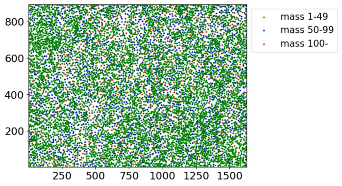
Figure 1: A sample of point configuration of center-of-masses of bushes in a desert. The sizes of area are indicated not by real lengths in meters but by numbers of pixels for the digital data; $L_{x}=1627$, $L_{y}=895$. The total number of points is $N=9853$ and the density is $\rho\fallingdotseq 6.77\times 10^{-3}$. The bush-size (mass) distribution is represented by colors of each points; the points with masses $1\leq M(\bm{X}_{j})\leq 49$ are green, the points with $50\leq M(\bm{X}_{j})\leq 99$ are blue, and the points with $M(\bm{X}_{j})\geq 100$ are red. See Section 3 how to produce such digital data.

In the present paper, we study the spatial distributions of bushes in deserts. In infertile lands plants can survive only if they have continued to beet the competitions to obtain sufficient amount of water and nutrition. It is expected that such survival competitions will cause strong and long-ranged repulsive interactions among plants. Figure 1 shows one sample of point process obtained from the real data of bushes distributed in the 2195.1 m $\times$ 1208.25 m area in a desert found in the Talampaya Natural Park in Argentina. There we plotted $N=9853$ points $\bm{X}_{j}\in\Lambda$, $j=1,2,\dots,N$, each of which gives the center-of-mass of a bush. As explained in detail in Section 3, we will define a size for each bush, which we call a mass and write as $M(\bm{X}_{j})$, $j=1,2,\dots,N$ in the present paper. We have obtained several real samples of point configurations of center-of-masses of bushes $\mathcal{P}=\{\bm{X}_{j}\}_{j=1}^{N}$ weighted by masses $\{M(\bm{X}_{j}):\bm{X}_{j}\in\mathcal{P}$} in deserts. Such weighted point configurations are called marked point processes in mathematical literature [2, 5]. The partial information of masses is shown by coloring of points in Fig. 1.

We can see in Fig. 1 that the point configuration tends to sparse around the points whose masses $M(\bm{X}_{j})\geq 100$ (the bushes with large sizes indicated by red points). On the other hand, the points with small masses $M(\bm{X}_{j})\leq 49$ (the bushes with small sizes indicated by green points) tend to be dense and make clusters. Therefore, if we ignore the mass data and only look at the point configuration of center-of-masses of bushes, the density fluctuation seems to be large. Such a situation is similar to PPP and we can not expect hyperuniformity. In the present paper, however, we show that if we take into account the mass data correctly, the sample of marked point process shown by Fig. 1 as well as some other samples obtained from the real data of bushes in deserts are in hyperuniform states at least in the observed scales.

As briefly explained in Section 2, there are some families of random unmarked point processes for which hyperuniformity is mathematically proved. To the knowledge of the present authors, however, there is no example of random marked point process such that it is proved to become hyperuniform if and only if the marks to points are taken into account. Moreover, random unmarked point processes having hyperuniformity, which have been well studied in mathematical physics, are all in Class I or Class II according to the classification by Torquato [33] (see Section 2.2 below). Our data analysis of marked point processes of bushes in deserts shows that if they are in hyperuniform states, then they seem to be in Class III.

In the present paper, we propose statistical mechanics models in non-equilibrium to generate random point configurations weighted by masses on a plane, which do not have hyperuniformity as unmarked point processes, but have hyperuniformity as marked point processes. In our models, we consider a stochastic processes to iterate random thinning of points [16, 17, 31] and coalescing (aggregation, clustering) of masses [8, 22, 25]. Our numerical simulations show that even if we start from PPP, a sufficiently large number of iterations of these two procedures generate non-trivial marked point processes having the desired properties. Comparisons with the real data of bushes are discussed.

The paper is organized as follows. In Section 2 we introduce mathematical expressions of random unmarked and marked point processes and give brief explanations of hyperuniformity. In Section 3 we explain how to produce digital data of weighted point configurations of bushes in deserts from the satellite images of the Google Maps. Then we introduce a procedure to measure hyperuniformity of the obtained data of finite sizes. There we report the results of our data analysis for hyperuniformity and mass distributions of several samples obtained from plural deserts. Section 4 is devoted to introducing our models to generate random marked point processes and to showing numerical analysis of universal property of hyperuniformity and non-universal property of mass distributions. We give discussions and concluding remarks in Section 5.

2 Mathematical Expressions

2.1 Marked and unmarked point processes

Consider a continuous space $S$; for example, the two-dimensional Euclidean space $S=\mathbb{R}^{2}$, which can be identified with the complex plane $S=\mathbb{C}$. We consider a set $\mathcal{P}=\{\bm{X}_{j}\}_{j\geq 1}$ consisting of points $\bm{X}_{j}\in S$, $j=1,2,\dots$, to represent a point configuration. For any point $\bm{x}\in S$, we introduce a Dirac measure (point mass) denoted by $\delta_{\bm{x}}$ [2, 5]. This is a function of any subset $B\subset S$ such that

$$\delta_{\bm{x}}(B)=\begin{cases}1,&\quad\mbox{if $\bm{x}\in B$},\\ 0,&\quad\mbox{otherwise}.\end{cases}$$ (2.1)

It is useful to represent the point configuration $\mathcal{P}$ by a sum of the Dirac measures as

$$\Xi(B)=\sum_{\bm{X}:\bm{X}\in\mathcal{P}}\delta_{\bm{X}}(B),$$ (2.2)

since (2.2) gives a total number of points included in $B$ for any subset $B\subset S$; $\Xi(B)=\sum_{\bm{X}:\bm{X}\in\mathcal{P}\cap B}1$. We call $\Xi$ associated with $\mathcal{P}$ a unmarked point process, or simply a point process. We also consider a marked point process, in which each point $\bm{X}\in\mathcal{P}$ carries a variable $M(\bm{X})$. Such a marked point process is denoted by

$$\Pi(B)=\sum_{\bm{X}:\bm{X}\in\mathcal{P}}M(\bm{X})\delta_{\bm{X}}(B),\quad B\subset S.$$ (2.3)

In this paper, we call $M(\bm{X})$ a mass of the point $\bm{X}\in\mathcal{P}$. For each subset $B\subset S$, (2.3) gives a total mass of the points included in $B$; $\Pi(B)=\sum_{\bm{X}:\bm{X}\in\mathcal{P}\cap B}M(\bm{X})$. From a marked point process $\Pi$, we can obtain a unmarked point process by deleting the information of masses of points. We denote the unmarked point process obtained from (2.3) as $\Xi_{\Pi}$ in this paper.

We consider two kinds of random unmarked point processes, the Poisson point process (PPP) and the Ginibre point process (GPP), which are well studied in probability theory and random matrix theory. We write samples of these random point processes as $\Xi^{\rm PPP}$ and $\Xi^{\rm GPP}$, respectively.

Remark 1   If we consider a pair of $\bm{X}_{j}\in S$ and $M(\bm{X}_{j})\in\mathbb{R}$ as a point $\widehat{\bm{X}}_{j}$ in the direct product space $S\times\mathbb{R}$; $(\bm{X}_{j},M(\bm{X}_{j}))\Leftrightarrow\widehat{\bm{X}}_{j}$, then (2.3) can be regarded as a usual point process in $S\times\mathbb{R}$ and written as $\Pi=\sum_{j}\delta_{\widehat{\bm{X}}_{j}}$ [2]. In the present paper, however, we call the point process which can be written in the form (2.3) a marked point process and the point process in the simpler form (2.2) as an unmarked point process in order to clearly distinguish these two types of point processes.

2.2 Three classes of hyperuniformity

Let $\Lambda_{\ell}$ be a subset of $S$ with a linear size $\ell>0$. Such a subset of $S$ is called a window in the study of hyperuniformity. The expectation of the number of unmarked points of $\Xi$ included in the window $\Lambda_{\ell}$ is written as $\langle\Xi(\Lambda_{\ell})\rangle$ and its variance is given by

$$\mathrm{Var}[\Xi(\Lambda_{\ell})]=\langle(\Xi(\Lambda_{\ell})-\langle\Xi(\Lambda_{\ell})\rangle)^{2}\rangle$$ (2.4)

Similarly, the expectation of the total mass of the marked points of $\Pi$ included in the window $\Lambda_{\ell}$ is written as $\langle\Pi(\Lambda_{\ell})\rangle$ and its variance is given by

$$\mathrm{Var}[\Pi(\Lambda_{\ell})]=\langle(\Pi(\Lambda_{\ell})-\langle\Pi(\Lambda_{\ell})\rangle)^{2}\rangle.$$ (2.5)

We consider the ratios,

$$R_{\ell}^{\mathrm{point}}:=\frac{\mathrm{Var}[\Xi(\Lambda_{\ell})]}{\langle\Xi(\Lambda_{\ell})\rangle},\quad R_{\ell}^{\mathrm{mass}}:=\frac{\mathrm{Var}[\Pi(\Lambda_{\ell})]}{\langle\Pi(\Lambda_{\ell})\rangle}.$$ (2.6)

We assume that the window will cover the whole space asymptotically, $\Lambda_{\ell}\to S$, as the linear size of window $\ell\to\infty$. If

$$\lim_{\ell\to\infty}R_{\ell}^{\sharp}=0,\qquad\mbox{$\sharp=$ mass or point},$$

then the point process is said to be hyperuniform. Torquato proposed three classes depending on the order of convergence to $0$ [33].

Class I:

$R_{\ell}^{\sharp}\simeq\ell^{-1}$ as $\ell\to\infty$. Example 1: GPP $\Xi^{\rm GPP}$ [24, 26, 27, 33]

$$S=\mathbb{R}^{2}\simeq\mathbb{C},\qquad\mbox{$\sharp=$ point}.$$

Example 2: Heisenberg family of determinantal point processes (DPPs) [18]

$$S=\mathbb{R}^{2D}\simeq\mathbb{C}^{D},\quad D\in\mathbb{N}\equiv\left\{1,2,...\right\},\qquad\mbox{$\sharp=$ point}.$$

Class II:

$R_{\ell}^{\sharp}\simeq\ell^{-1}\log\ell$ as $\ell\to\infty$. Example 3: sinc (sine) DPP [4, 19, 28, 29, 30],

$$S=\mathbb{R},\qquad\mbox{$\sharp=$ point}.$$

Example 4: Euclidean family of DPPs [12]

$$S=\mathbb{R}^{d},\quad d\in\mathbb{N},\qquad\mbox{$\sharp=$ point}.$$

Class III:

$R_{\ell}^{\sharp}\simeq\ell^{-\alpha},\ 0<\alpha<1$  as $\ell\to\infty$.

3 Data Production and Numerical Analysis of Point Processes

3.1 Bush distributions in deserts

First we explain how to produce digital data of point configurations of bushes in a desert. From now on, the size of the digital data of the point configuration is written as $L_{x}\times L_{y}$. and the total number of points is $N$. We define the aspect ratio as $\lambda=L_{y}/L_{x}$.

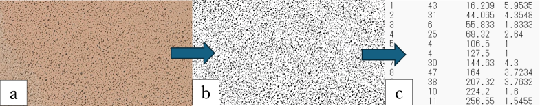
Figure 2: Image processing. The Google Maps satellite image (a) was converted to a gray-scale image (b) by the software Image J, and then the digital data (c) was produced by Matlab.

The center-of-mass coordinates and sizes were obtained for bushes in deserts by the following procedure: Here we explain the procedure using the example of a desert in the Talampaya Natural Park in Argentina.

   (i)

A rectangular area was cut out from the Google Maps satellite image of a part of desert. In this example, the rectangular area is an image of a part of the desert centered at the point ($29^{\circ}56^{\prime}02.2^{\prime\prime}\text{S},67^{\circ}50^{\prime}13.6^{\prime\prime}\text{W}$) with length of $2195.1$ m in the east-west (EW) direction and length of $1208.25$ m in the north-south (NS) direction. Bushes are dotted with a variety of sizes as shown in Fig.2 (a).

   (ii)

The image was converted to be gray-scaled using the average method in the computer software Image J. Figure 2 (b) is the result obtained from Fig.2 (a). The resolution of this image is $L_{x}=1626$ pixels by $L_{y}=895$ pixels, which means that each individual pixel corresponds to a geographical area of about $1.35$m $\times$ $1.35$m.

   (iii)

The obtained gray-scaled image was then binarized by automatically setting the threshold value and using the Otsu method, also in Image J. Each pixel is binarized as follows:

dark pixel (bush) $$\longrightarrow\mbox{black pixel (mass $=1$)},$$

light pixel (non-bush) $$\longrightarrow\mbox{white pixel (mass $=0$)}.$$

   (iv)

The number of black pixels forming a cluster (connected component) was counted as a mass of each bush. By averaging of coordinates of the black pixels included in a cluster, the $x$- and $y$-coordinates of the center-of-mass was calculated for each bush. This procedure was done by Matlab image recognition. Figure 2 (c) shows a part of the obtained table which lists out the identification numbers of the bushes, the masses, the x-coordinates, and the y-coordinates of the center-of-masses.

Figure 1 in Section 1 demonstrated the obtained digital data of configuration of bushes in a desert in the Talampaya Natural Park in Argentina. The sizes of the area are given in pixel unit as $L_{x}=1626$ and $L_{y}=895$. There $N=9853$ dots are plotted, each of which indicates the location of center-of-mass of a bush. Each dot $\bm{X}_{j}$, $j=1,2,\dots,N$, has a data of mass $M(\bm{X}_{j})\in\{1,2,\dots\}$. In Fig, 1, however, only partial information of masses is shown by coloring of dots by green for $1\leq M(\bm{X}_{j})\leq 49$, by blue for $50\leq M(\bm{X}_{j})\leq 99$, and by red for $M(\bm{X}_{j})\geq 100$.

Table 1: Data of samples studied in this paper. The areas of Nos.1–5 are in the Talampaya Natural Park, La Rioja, Argentina, Nos.5 and 6 in the Parc culturel national de Tindouf, Oum El Assel, Algeria, No. 7 at Flying Fox, Northrm Territory, Australia, and No. 8 at Maikona, Kenya. The latitude and longitude are for the center of each area. Real sizes in the east-west (EW), and north-south (NS) directions are given in the metric unit, whose pixels in the digital data are also shown. The total number of bushes in each area is given by $N$. The areas of Algeria 1, 2 are found in a Wadi and hence the aspect ratios $\lambda=\Lambda_{y}/\Lambda_{x}$ are quite deviated from 1.

No.	name	location of center		size in meters		size in pixels		$N$
		latitude	longitude	EW	NS	$L_{x}$	$L_{y}$
1	(Argentina) bush 1	$29^{\circ}56^{\prime}02.2^{\prime\prime}$S	$67^{\circ}50^{\prime}13.6^{\prime\prime}$W	2195	1208	1626	895	9853
2	(Argentina) bush 2	$29^{\circ}55^{\prime}51.5^{\prime\prime}$S	$67^{\circ}50^{\prime}13.6^{\prime\prime}$W	2160	1080	1600	800	9083
3	(Argentina) bush 3	$29^{\circ}56^{\prime}02.0^{\prime\prime}$S	$67^{\circ}49^{\prime}50.1^{\prime\prime}$W	2160	1080	1600	800	10896
4	(Argentina) bush 4	$29^{\circ}56^{\prime}12.3^{\prime\prime}$S	$67^{\circ}50^{\prime}13.5^{\prime\prime}$W	2160	1080	1600	800	10034
5	(Argentina) bush 5	$29^{\circ}56^{\prime}02.6^{\prime\prime}$S	$67^{\circ}50^{\prime}39.5^{\prime\prime}$W	2160	1080	1600	800	10249
6	Algeria 1	$28^{\circ}48^{\prime}00.3^{\prime\prime}$N	$6^{\circ}23^{\prime}42.5^{\prime\prime}$W	1786	198	1323	147	948
7	Algeria 2	$28^{\circ}48^{\prime}15.1^{\prime\prime}$N	$6^{\circ}24^{\prime}12.5^{\prime\prime}$W	201	2165	149	1604	816
8	Australia	$14^{\circ}34^{\prime}41.4^{\prime\prime}$S	$133^{\circ}31^{\prime}41.1^{\prime\prime}$E	2160	1080	1600	800	3597
9	Kenya	$3^{\circ}31^{\prime}00.1^{\prime\prime}$N	$38^{\circ}12^{\prime}24.3^{\prime\prime}$E	2160	1080	1600	800	10660

We will call the sample shown by Fig, 1 simply (Argentina) bush 1 in the following. By the similar procedure explained above, we have prepared other four samples from the same desert in Argentina, two samples from a desert in Algeria, one from Australia, and one from Kenya. The detailed data are listed out in Table 1.

3.2 Poisson point process and Ginibre point process

In order to compare the statistics, here we make two digital data of the Poisson point process (PPP) and the Ginibre point process (GPP) with approximately the same number of points $N$ and the same sizes $L_{x}\times L_{y}$ with the sample bush 1. Notice that they are both unmarked point processes.

PPP is a completely random configuration of points [2, 5]. For each point $\bm{X}_{j}=(X_{j},Y_{j})$, the coordinates $X_{j}$ and $Y_{j}$ are chosen independently from a uniform distributions in $[0,L_{x}]$ and $[0,L_{y}]$, respectively. We repeat the random choosing of point $N$ times independently. Figure 3 shows an obtained sample for $L_{x}=1626$, $L_{y}=895$, and $N=9853$. The density is $\rho\fallingdotseq 6.771\times 10^{-3}$. The obtained PPP is denoted by $\Xi^{\rm PPP}$.

GPP is obtained by the eigenvalue distribution of a non-Hermitian random matrix on a complex plane [7]. We consider an $n\times n$ matrix $Z_{n}$ as follows,

$$Z_{n}:=\begin{bmatrix}\frac{1}{\sqrt{2}}(X_{11}+iY_{11})&\cdots&\frac{1}{\sqrt{2}}(X_{1n}+iY_{1n})\\ \vdots&\ddots&\vdots\\ \frac{1}{\sqrt{2}}(X_{n1}+iY_{n1})&\cdots&\frac{1}{\sqrt{2}}(X_{nn}+iY_{nn})\end{bmatrix},$$

where $i=\sqrt{-1}$. Here $X_{jk}$ and $Y_{jk}$, $j,k=1,2,\dots,n$ are i.i.d. following the standard normal distribution $\mathrm{N}(0,1)$, that is, the Gaussian distribution with mean zero and variance $\sigma^{2}=1$. It is known as the circular law such that the $n$ eigenvalues of $Z_{n}$ are not degenerated and uniformly distributed in a disk centered at the origin with radius $\sqrt{n}$, if $n$ is sufficiently large [6, 19]. The circular law implies that the density of GPP is

$$\rho_{\mathrm{G}}=\frac{n}{\pi(\sqrt{n})^{2}}=\frac{1}{\pi}.$$

Inside of the disk, we prepare a rectangular region $L_{x}^{0}\times L_{y}^{0}$ with the aspect ratio $L_{y}^{0}/L_{x}^{0}=\lambda$ so that it contains $N$ eigenvalues. These conditions determine that

$$\rho_{\mathrm{G}}L_{x}^{0}L_{y}^{0}=N\ \Longrightarrow\ L_{x}^{0}=\sqrt{\frac{N\pi}{\lambda}}.$$ (3.7)

If we put $N=9853$ and $\lambda=L_{x}/L_{y}=1626/895$, (3.7) gives

$$L_{x}^{0}=\sqrt{\frac{N\pi}{\lambda}}=\sqrt{N\pi\frac{L_{x}}{L_{y}}}\fallingdotseq 237.1.$$

In our numerical calculation, we have used $Z_{n}$ with $n=2.2\times 10^{4}$. Hence we see $237.1<2\sqrt{n}\fallingdotseq 296$, and confirmed that the matrix size is large enough for our purpose. Then we dilate the obtained point configuration in the region $L_{x}^{0}\times L_{y}^{0}$ to that in $L_{x}\times L_{y}$; that is, the size of region is enlarged by linear factor $L_{x}/L_{x}^{0}\fallingdotseq 6.857$. The obtained sample is shown by Fig.3 (b). The expected density of dots is $\rho=(1/\pi)\times 6.857^{-2}\fallingdotseq 6.770\times 10^{-3}$. The exact number of points in Fig.3 (b) is 9862, which has a small deviation from the target number $N=9862$ due to a sample fluctuation and the finite-size effect of matrix. But this deviation is negligible in our scaling analysis mentioned below. The obtained GPP is denoted by $\Xi^{\rm GPP}$.

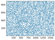
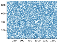
(a) Poisson point process $\Xi^{\rm PPP}$

(b) Ginibre point process $\Xi^{\rm GPP}$

Figure 3: Numerically obtained samples of PPP and GPP. Both are prepared in the region $L_{x}\times L_{y}=1626\times 895$ with density $\rho\fallingdotseq 6.77\times 10^{-3}$ matched with the digital data for bush 1 shown by Fig. 1.

We can see clear difference between PPP and GPP in Fig. 3. Sparseness found in PPP is much suppressed in GPP. As already mentioned in previous sections, GPP is hyperuniform, while PPP is not. If we ignore the coloring of points in Fig. 1 for bush 1, the point configuration seems to be similar to PPP. The problem is how about the point configuration if we take into account the information of masses of bushes. Is it possible to be in hyperuniform state as a marked point process? The answer is positive as explained below.

3.3 Measurements of hyperuniformity by finite-size data

We prepare a series of windows parameterized by linear size $\ell$, $\{\Lambda_{\ell}\}$, such that $\Lambda_{\ell}$ expands monotonically as $\ell$ increases and $\Lambda_{\ell}$ will cover the whole space asymptotically in the limit $\ell\to\infty$. As explained in Section 2.2, the hyperuniformity of random point process is defined and classified mathematically by asymptotices in the limit $\ell\to\infty$ of the ratio $R_{\ell}$ of the variance with respect to the expectation concerning the number of points included $\Lambda_{\ell}$. In real experiments of physics as well as observation in ecological systems, however, we have only a few number of sample configurations in finite regions.

On the other hand, two samples of point processes given by Fig. 3 can be distinguished from each other, since they represent typical properties of uncorrelated and fluctuating point configuration in space in Fig. 3 (a) and of correlated point configuration where fluctuation is suppressed to keep hyperuniformity in Fig. 3 (b). By such observations, here we propose a numerical method to measure hyperuniformity using only one but typical sample of point processes observed in nature. We adopted two strategies; (i) Instead of observing the asymptotics in large-scale limit, we divide a given finite system into smaller subsystems systematically. (ii) Instead of averaging over many samples, we average the data over subsystems obtained by division of one sample.

We consider a rectangular region $L_{x}\times L_{y}$, We fix the aspect ratio $\lambda=L_{y}/L_{x}$ and write it simply as $\Lambda_{L_{x}}$ putting only the size in the $x$-direction as a subscript. Let $m\in\mathbb{N}$ and we divide $\Lambda_{L_{x}}$ into $m\times m$ subregions. The lengths in the $x$- and $y$-directions are then given by

$$\ell_{x}=L_{x}/m,\quad\ell_{y}=L_{y}/m.$$

The obtained subregions are labeled by $j=1,2,\dots,m^{2}$ as

$$\Lambda_{L_{x}}\quad\Longrightarrow\quad\left\{\Lambda_{\ell_{x}}^{1},\Lambda_{\ell_{x}}^{2},\dots,\Lambda_{\ell_{x}}^{m^{2}}\right\}.$$

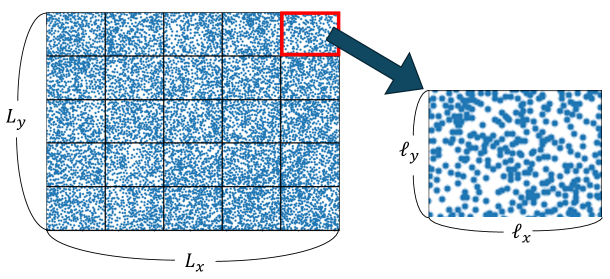
Figure 4: The region $L_{x}\times L_{y}$ on which a sample of point process is given is divided into $m\times m$ subdomains. Each subregion is a similar rectangular $\ell_{x}\times\ell_{y}$ denoted by $\Lambda_{\ell_{x}}^{j}$, $j=1,2,\dots,m^{2}$. The case with $m=5$ is shown.

First we consider an unmarked point process $\Xi(\Lambda_{L_{x}})$. Examples are the point configurations of center-of-mass coordinates of bushes in a desert $\Xi_{\Pi}$ for which the mass information is deleted, $\Xi^{\rm PPP}$, and $\Xi^{\rm GPP}$. For all $j=1,2,\dots,m^{2}$, the expectation of $\Xi(\Lambda_{\ell_{x}}^{j})$ is simply evaluated as $\langle\Xi(\Lambda_{\ell_{x}}^{j})\rangle\equiv\rho\ell_{x}\ell_{y}$, where $\rho$ is the density of points of the given sample $\Lambda_{L_{x}}$, $\rho=\Xi(\Lambda_{L_{x}})/(L_{x}L_{y})=N/(L_{x}L_{y})$. Then for each subregion $\Lambda_{\ell_{x}}^{j}$, $j=1,2,\dots,m^{2}$, we count the deviation of number of points observed in it from the expectation, and define the variance by the following arithmetic mean over $m^{2}$ subregions,

$$\mathrm{Var}[\Xi(\Lambda_{\ell_{x}})]=\frac{1}{m^{2}}\sum_{j=1}^{m^{2}}\left(\Xi(\Lambda_{\ell_{x}}^{j})-\rho\ell_{x}\ell_{y}\right)^{2}.$$ (3.8)

The ratios of the variances with respect to expectations are written as $R^{\rm point}_{\ell_{x}}$ for unmarked point process of bush configurations $\Xi_{\Pi}$, $R^{\rm PPP}_{\ell_{x}}$ for $\Xi^{\rm PPP}$, and $R^{\rm GPP}_{\ell_{x}}$ for $\Xi^{\rm GPP}$;

$$R^{\rm point}_{\ell_{x}}=\frac{\mathrm{Var}[\Xi_{\Pi}(\Lambda_{\ell_{x}})]}{\rho\ell_{x}\ell_{y}},\quad R^{\rm PPP}_{\ell_{x}}=\frac{\mathrm{Var}[\Xi^{\rm PPP}(\Lambda_{\ell_{x}})]}{\rho\ell_{x}\ell_{y}},\quad R^{\rm GPP}_{\ell_{x}}=\frac{\mathrm{Var}[\Xi^{\rm GPP}(\Lambda_{\ell_{x}})]}{\rho\ell_{x}\ell_{y}}.$$ (3.9)

Next we consider an marked point process $\Pi(\Lambda_{L_{x}})$. Examples are the point configurations of center-of-mass coordinates of bushes in a desert $\Xi_{\Pi}$ weighted by masses. Instead of the density of point $\rho$, here we calculate the density of mass defined by

$$\rho^{\rm mass}=\frac{\Pi(\Lambda_{L_{x}})}{L_{x}L_{y}}=\frac{\sum_{\bm{X}:\bm{X}\in\mathcal{P}\cap\Lambda_{L_{x}}}M(\bm{X})}{L_{x}L_{y}}.$$

For all $j=1,2,\dots,m^{2}$, the expectation of $\Pi(\Lambda_{\ell_{x}}^{j})$ is evaluated as $\langle\Xi(\Pi_{\ell_{x}}^{j})\rangle\equiv\rho^{\rm mass}\ell_{x}\ell_{y}$. Then the variance is calculated as

$$\mathrm{Var}[\Pi(\Lambda_{\ell_{x}})]=\frac{1}{m^{2}}\sum_{j=1}^{m^{2}}\left(\Pi(\Lambda_{\ell_{x}}^{j}))-\rho^{\rm mass}\ell_{x}\ell_{y}\right)^{2}.$$ (3.10)

The ratio of the variance with respect to expectation is written as $R^{\rm mass}_{\ell_{x}}$ for bush configurations weighted by masses;

$$R^{\rm mass}_{\ell_{x}}=\frac{\mathrm{Var}[\Pi(\Lambda_{\ell_{x}})]}{\rho^{\rm mass}\ell_{x}\ell_{y}}.$$ (3.11)

3.4 Hyperuniformity of marked point processes of bushes in a desert in Argentina

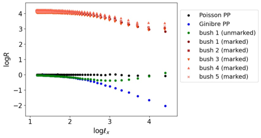
(a) Log-log plots of $R_{\ell_{x}}$ versus $\ell_{x}$ for various unmarked and marked point processes. The bush configuration not taking into account of mass information does not show hyperuniformity similarly to PPP, while the bush configurations weighted by masses exhibit hyperuniformity similarly to GPP.

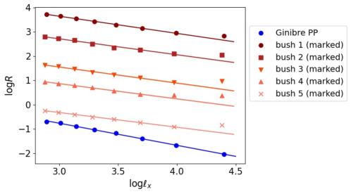
(b) Linear fitting to (3.12) were performed for the interval of $X\equiv\log\ell_{x}$ such that $2.8\leq X\leq 4.4$ for GPP, $2.8\leq X\leq 4.0$ for the marked point processes of bush 1-3 and 5, and $2.8\leq X\leq 3.8$ for bush 4. The fitting works well and the exponent $\alpha$ is evaluated as (3.13). Here the dots are shifted in the direction of $Y\equiv\log R$ by $-(n-1)$ for each bush n, $n=1,2,\dots,5$, respectively, to avoid overlaps of plots and fitting lines.

Figure 5: Numerical measurements of hyperuniformity using finite-size data

In Fig. 5 (a), we show dependence on $\log\ell_{x}$ of logarithms of $R^{\rm point}_{\ell_{x}}$ for the unmarked point configurations of the sample bush 1, $\log R^{\rm PPP}_{\ell_{x}}$ and $\log R^{\rm GPP}_{\ell x}$. For the totally five samples from the desert in Argentina, bush 1–5 in Table 1, $\log R^{\rm mass}_{\ell_{x}}$ are also plotted versus $\log\ell_{x}$, which are marked point processes in Fig. 5 (a). In the numerical measurements of variances by (3.8) and (3.10) in Section 3.3, the numbers of subregions $m$ become relatively small for large values of $\ell_{x}$, and hence the obtained plots are scattered. For this reason we only use the data with $\log\ell_{x}<4.5$.

With increment of the window size $\ell_{x}$, the number fluctuation $R^{\rm PPP}_{\ell_{x}}$ does not show any decay, while $R^{\rm GPP}_{\ell_{x}}$ shows a systematic decay. These plots suggest that $\Xi^{\rm PPP}$ has no hyperuniformity, but $\Xi^{\rm GPP}$ is in a hyperuniform state, as expected. We see that the behavior of $\log R^{\rm point}_{\ell_{x}}$ versus $\log\ell_{x}$ of unmarked point processes of bush 1 is very similar to that of PPP, as already observed in Fig. 5 (a) It implies that if the mass is not taken into account, any hyperuniformity can not be observed in bush configurations in the desert. If we consider the marked point processes, however, in which each point is weighted by mass, linear decay of $\log R^{\rm pass}_{\ell_{x}}$ with increment of $\ell_{x}$ is commonly observed as shown by the five data from the desert in Argentina, bush 1–5 (marked) in Fig. 5 (a).

Figure 5 (b) shows the results of the linear fitting,

$$\log R_{\ell_{x}}=-\alpha\log\ell_{x}+c,$$ (3.12)

for GPP $\Xi^{\rm GPP}$, and bush 1–5. Here in order to avoid overlaps of plots and fitting lines, the data points are shifted in the $Y$-direction by $-(n-1)$ for data, bush n, $n=1,2,\dots,5$. The numerically estimated values of exponent $\alpha$ are the following; $\alpha^{\rm GPP}=0.91\fallingdotseq 1$, $\alpha^{\rm bush\,1}=0.71$, $\alpha^{\rm bush\,2}=0.66$, $\alpha^{\rm bush\,3}=0.66$, $\alpha^{\rm bush\,4}=0.63$, and $\alpha^{\rm bush\,5}=0.61$. The present numerical analysis suggest that the bush configurations weighted by masses sampled from the desert in Argentina are in the hyperuniform state of Class III,

$$R_{\ell_{x}}^{\rm mass}\simeq\ell_{x}^{-\alpha^{\rm Argentina}}\quad\mbox{with}\quad\alpha^{\rm Argentina}\fallingdotseq 0.65.$$ (3.13)

3.5 Mass distributions of marked point processes of bushes

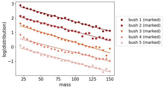
Figure 6: Semi-log plots of bush-mass distributions in bush 1–5. The dots are shifted in the direction of $\log$(distribution) by $-0.7(n-1)$ for each bush n, $n=1,2,\dots,5$, respectively, to avoid overlaps of plots and fitting lines. The linear fitting to (3.14) works well in the shown interval of mass, which gives $m_{0}^{\rm bush\,1}=76$, $m_{0}^{\rm bush\,2}=79$, $m_{0}^{\rm bush\,3}=69$, $m_{0}^{\rm bush\,4}=83$, $m_{0}^{\rm bush\,5}=78$.

For the marked point processes of bush 1–5, we have measured the mass distributions. Figure 6 shows the semi-log graphs for histograms of $M$. The results suggest that the mass distributions are well described by the exponential distribution,

$${\rm Prob}(M\in[m,m+dm))\simeq e^{-m/m_{0}}dm\quad\mbox{with}\quad m_{0}^{\rm Argentina}\fallingdotseq 77.$$ (3.14)

3.6 Hyperuniformity of other deserts

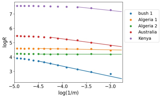
Figure 7: Logarithms of $R^{\rm mass}$ are plotted as functions of $\log(1/m)$ for a variety of samples from different deserts. Linear fitting gives the exponent $\alpha$.

Figure 7 shows logarithms of the ratios $R^{\rm mass}$ as functions of $\log(1/m)$ for the samples in deserts Nos.6–9 as well as for the bush 1 given as No.1 in Table 1, where $m$ is the number of divisions of the finite-size data as explained in Section 3.3. The linear fitting to $\log R=-\alpha\log(1/m)+c$ gives the exponents $\alpha^{\rm Algeria\,1}=0.062$, $\alpha^{\rm Algeria\,2}=0.0049$, $\alpha^{\rm Australia}=0.44$, and $\alpha^{\rm Kenya}=0.36$. The marked point processes obtained from the desert in Algeria (sample Nos.6 and 7) do not show hyperuniformity ($\alpha^{\rm Algeria}\fallingdotseq 0$), while those from Australia (No.8) and Kenya (No.9) seem to be in the hyperuniform state in Class III, where the values of the exponent $\alpha$ are smaller than $\alpha^{\rm Argentina}\fallingdotseq 0.65$.

4 Models

4.1 Random thinning-coalescing processes

For a rectangular region with aspect ratio $\lambda$, $\Lambda_{L_{x}}=\left\{(x,y)\in\mathbb{R}^{2}:0\leq x\leq L_{x},0\leq y\leq\lambda L_{x}\right\}$, we define an extended region with $r>0$ by

$$\Lambda_{L_{x},r}:=\left\{(x,y)\in\mathbb{R}^{2}:-2r\leq x\leq L_{x}+2r,-2r\leq y\leq\lambda L_{x}+2r\right\}\supset\Lambda_{L_{x}}.$$

For two points $\bm{X}=(X_{x},X_{y})$, $\bm{Y}=(Y_{x},Y_{y})\in\Lambda_{L_{x},r}$, the distance is defined by $d(\bm{X},\bm{Y})=\sqrt{(X_{x}-Y_{x})^{2}+(X_{y}-Y_{y})^{2}}$. Give a probability density ${p(a)}$ for a non-negative random variable ${A}$ so that

$$P(A\leq a)=\int_{0}^{a}p(a^{\prime})da^{\prime},$$ (4.15)

and the mean is finite; $a_{0}:=\langle A\rangle=\int_{0}^{\infty}p(a^{\prime})da^{\prime}<\infty$. Let $r_{0}:=\sqrt{a_{0}/\pi}$.

We consider the following transformation $\mathcal{T}$ of the marked point process on $\Lambda_{L_{x},r_{0}}$,

$$\mathcal{T}:\Pi(B)=\sum_{\bm{X}:\bm{X}\in\mathcal{P}}M(\bm{X})\delta_{\bm{X}}(B)\quad\Longrightarrow\quad\widetilde{\Pi}(B)=\sum_{\bm{X}:\bm{X}\in\widetilde{\mathcal{P}}}\widetilde{M}(\bm{X})\delta_{\bm{X}}(B),$$

where $B$ is an arbitrary subregion of $\Lambda_{L_{x}}$.

(1)

Choose a point $\bm{X}$ randomly from the set of points $\mathcal{P}$ which are included in $\Lambda_{L_{x}}$; $\bm{X}\in\mathcal{P}\cap\Lambda_{L_{x}}$.

(2)

Let ${A}$ be a non-negative random variable following the probability law (4.15) and set ${R:=\sqrt{A/\pi}}$. That is, $R$ is the radius of a disk whose area is equal to $A$. For a chosen point $\bm{X}$, define a subset of $\mathcal{P}$ by

$$\mathcal{P}(\bm{X}):=\{\bm{Y}\in\mathcal{P}\backslash\left\{\bm{X}\right\}:d(\bm{X},\bm{Y})\leq R\}.$$

Notice that $\mathcal{P}(\bm{X})$ is a collection of all points except $\bm{X}$, which are included in the disk centered at $\bm{X}$ with radius $R$.

(3)

Set

$$\widetilde{\mathcal{P}} =\mathcal{P}\backslash\mathcal{P}(\bm{X}),$$ (4.16)

$$\widetilde{M}(\bm{Z}) =\begin{cases}\displaystyle{M(\bm{X})+\sum_{\bm{Y}:\bm{Y}\in\mathcal{P}(\bm{X})}M(\bm{Y})},&\mbox{if ${\bm{Z}=\bm{X}}$}\cr M(\bm{Z}),&\mbox{if ${\bm{Z}\in\widetilde{\mathcal{P}}\backslash\left\{\bm{X}\right\}}$}.\end{cases}$$ (4.17)

The reduction of points (4.16) represents a random thinning [16, 17, 31]. That is, all points except $\bm{X}$ included in a disk centered at $\bm{X}$ with radius $R$ are deleted. Then the first line of (4.17) represents coalescing (aggregation, clustering) of masses of the deleted points into the chosen point $\bm{X}$ [8, 22, 25]. As reported in the following, we have iterated the transformation ${\mathcal{T}}$, where the times of iterations is written as $T$. We have found that even though the initial marked point process has no hyperuniformity, if we iterate the transformation $\mathcal{T}$ sufficiently many times, $T\gg 1$, then we can obtain non-trivial marked point process having hyperuniformity.

4.2 Results of numerical simulations

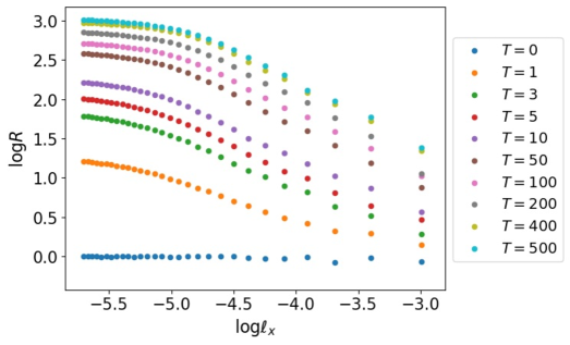
Figure 8: Dependence on the number of iterations $T$ is shown in the $\log R_{\ell_{x}}$ versus $\log\ell_{x}$ plots, where $L=L_{x}=L_{y}=4000$ and $a_{0}\equiv\theta_{0}=1000$ for (4.18).

Based on the observations in bush 1–5 reported in Section 3.5 such that the distribution of mass $M$ is well approximated by the exponential distribution, first we choose the exponential distribution for $A$, since the mass transform $M$ in each coalescing (4.17) will be given by the area $A$ multiplied by density of points. The probability density function in (4.15) is assume to be given by

$$p(a)=p(a;\theta_{0})=\frac{1}{\theta_{0}}e^{-a/\theta_{0}},$$ (4.18)

where $\theta_{0}$ is the scale parameter. It is easy to verify that $\langle A\rangle=\theta_{0}\equiv a_{0}$ and $\mathrm{Var}[A]=\theta_{0}^{2}$. For simplicity, in the computer simulations of our model, we fix the aspect ratio $\lambda=1$; that is, $L_{x}=L_{y}\equiv L$.

Let $L=4000$ and $a_{0}=1000$. Starting from a sample of PPP obtained in Section 3.2, we have iterated the transformation $\mathcal{T}$. For each number of iterations $T$, we have performed the measurements explained in Section 3.3. The $\log R_{\ell_{x}}$ versus $\log\ell_{x}$ plots are given in Fig. 8 from $T=0$ (the initial PPP) to $T=500$. As $T$ increases, the value of $\log R_{\ell_{x}}$ increases and the region of $\log\ell_{x}$ in which $\log R_{\ell_{x}}$ shows a linear decay seems to extend. Moreover, we have observed convergence of the plots when $T\gtrsim 500$. We also confirmed the convergence of the plots to the same curve in the simulations starting from a sample of GPP prepared in Section 3.2. From now on, we will report the results of numerical simulations, which were obtained after $T=500$ iterations of the transformation $\mathcal{T}$.

4.2.1 Hyperuniformity

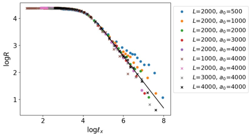
(a) The results for the marked point processes. As $L$ and $a_{0}$ increase, the linear region extends systematically.

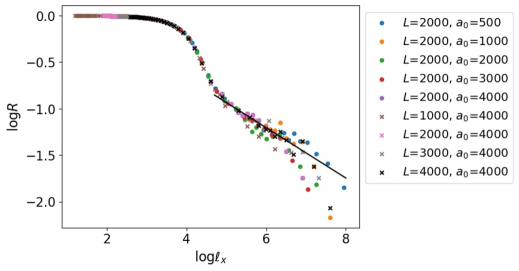
(b) The results for the unmarked point processes. Even if the values of $L$ and $a_{0}$ become large, the linear region seems to be restricted in a narrow region of scale.

Figure 9: $\log R_{\ell_{x}}$ versus $\log\ell_{x}$ of the point processes obtained by numerical simulation of the model with variety of system sizes $L=L_{x}=L_{y}$ and $a_{0}$.

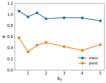
Figure 10: The estimated values of $\alpha$ for marked (mass) and unmarked (point) configurations obtained by the present algorithms with different shape parameters $k_{0}$ of the Gamma distribution for $A$. We see that $\alpha^{\rm model}_{\rm mass}\fallingdotseq 1$ and $\alpha^{\rm model}_{\rm point}\fallingdotseq 0.4$.

Both of the marked point processes $\Pi$ and the corresponding unmarked point processes $\Xi_{\Pi}$ obtained by our computer simulations are systematically studied by changing the system size $L$ and the mean value $a_{0}$ of the random area $A$. Figure 9 (a) shows the $\log R^{\rm mass}_{\ell_{x}}$ versus $\log\ell_{x}$ plots averaged over 20 marked point processes obtained by our model. For fixed $L=2000$, as $a_{0}$ increases from 500 to 4000, the linear region extends systematically. For the largest value $a_{0}=4000$, the linear region also systematically extends as $L$ increases from 1000 to 4000. By these results, we think that if both of $L$ and $a_{0}$ are sufficiently large, and if the number of iterations $T$ of the transformation $\mathcal{T}$ is large enough, our procedure produced marked point processes with hyperuniformity. The linear fitting (3.12) to the plots for $L=4000$ and $a_{0}=4000$ gives

$$R_{\ell_{x}}^{\rm mass}\simeq\ell_{x}^{-\alpha^{\rm model}_{\rm mass}}\quad\mbox{with}\quad\alpha^{\rm model}_{\rm mass}\fallingdotseq 0.96.$$ (4.19)

Figure 9 (b) shows the $\log R^{\rm point}_{\ell_{x}}$ versus $\log\ell_{x}$ plots averaged over 20 unmarked point processes, which are obtained from the marked point processes by deleting the data of mass distributions. Compared with $\log R^{\rm mass}_{\ell_{x}}$, even if the values of $L$ and $a_{0}$ become large, the linear region seems to be restricted in a narrow region of scale. The linear fitting (3.12) to the plots for $L=4000$ and $a_{0}=4000$ gives

$$R_{\ell_{x}}^{\rm point}\simeq\ell_{x}^{-\alpha^{\rm model}_{\rm point}}\quad\mbox{with}\quad\alpha^{\rm model}_{\rm point}\fallingdotseq 0.27.$$ (4.20)

We have studied dependence of the results on the choice of distribution (4.15) of random area $A$. As extensions of the exponential distribution (4.18), we consider the cases in which the area $A$ follows the Gamma distributions with the probability density

$$p(a)=p(a;k_{0},\theta_{0})=\frac{1}{\Gamma(k_{0})\theta_{0}^{k_{0}}}a^{k_{0}-1}e^{-a/\theta_{0}},$$ (4.21)

where $\Gamma(k)$ is the Gamma function, $\Gamma(k)=\int_{0}^{\infty}t^{k-1}e^{-t}dt$, and $k_{0}$ and $\theta_{0}$ are the shape and scale parameters, respectively. It is easy to verify that $\langle A\rangle=k_{0}\theta_{0}\equiv a_{0}$ and $\mathrm{Var}[A]=k_{0}\theta_{0}^{2}$. In particular, when $k_{0}=1$, (4.21) is reduced to the probability density of exponential distribution (4.18). When $k_{0}=n\in\mathbb{N}$, the Gamma distribution is called the Erlang distribution with probability density $p_{0}(a;n,\theta_{0})=a^{k_{0}-1}e^{-a/\theta_{0}}/[(n-1)!\theta_{0}^{n}]$, and when $k_{0}=n/2$ with $n\in\mathbb{N}$, it is related to the $\chi^{2}$ distribution. The marked point processes are generated by the present algorithms using the Gamma distributions with the shape parameters $k_{0}=$0.5, 1, 1.5, 2, 3, 4, and 5. The evaluated values of the exponent $\alpha$ are shown in Fig.10. The exponent $\alpha$ seems to be

$$\alpha^{\rm model}_{\rm mass}\fallingdotseq 1,\quad\alpha^{\rm model}_{\rm point}\fallingdotseq 0.4.$$ (4.22)

Remark 2   As a simplified model, we have simulated the algorithm with a fixed value of area $A$ of disk. Then we found that the number of iterations $T$ needed for convergence of point processes became much larger than 500. In addition, the convergence of the $\log R_{\ell_{x}}$–$\log\ell_{x}$ plots to a line needed larger values of $L$ and $a_{0}$ compared to the results shown by Fig. 9. Hence we have concluded that the randomness of area $A$ of disk is important to generate marked point processes with hyperuniformity efficiently.

4.2.2 Mass distributions

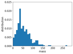
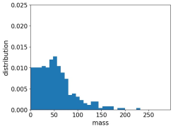
(a)

(b)

Figure 11: Two samples of mass distributions obtained by numerical simulations with $L=2000$ and $a_{0}=4000$. The example (a) shows a peak around 40 in the histogram, but the sample (b) shows a plateau under 50. The mass distributions depend on samples.

For Figs. 9 (a) and (b), we have performed 20 sets of the $T=500$ iterations of transformation $\mathcal{T}$ starting from independently obtained 20 samples of PPPs. We found that the mass distributions of 20 samples seem to be quite different from each other, especially when $a_{0}$ becomes large. Figure 11 shows two samples of mass distributions obtained by numerical simulations with $L=2000$ and $a_{0}=4000$. The mass distributions depend heavily on samples and they do not seem to be universal.

Nevertheless, if we average the mass distributions over 20 samples, the obtained curves are well approximated by the Gamma distributions with appropriate values of parameters

$$p_{\rm G}(m) =p_{\rm G}(m;k_{\rm G},\theta_{\rm G})$$

$$=\frac{1}{\Gamma(k_{\rm G})\theta_{\rm G}^{k_{\rm G}}}m^{k_{\rm G}-1}e^{-m/\theta_{\rm G}},\quad m\geq 0.$$ (4.23)

Here we have fixed the parameters of (4.21) for the model as $a_{0}=4000$ and $L=2000$. The $k_{0}$-dependence of the fitting curves of (4.23) are shown in Fig.12, where fitting parameters $(k_{\rm G},\theta_{\rm G})$ are given by $(2.15,39.29)$, $(2.2,24.26)$, $(2.5,21.6)$, $(2.5,18.13)$, $(2.55,14.48)$, $(2.6,13.0)$, and $(2.6,12.0)$ for $k_{0}=0.5,1,1.5,2,3,4$, and 5, respectively.

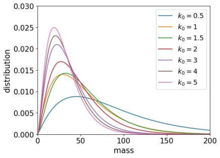
Figure 12: The mass distributions averaged over the 20 samples are calculated for several values of $k_{0}$ of the distribution (4.21). Here $L=2000$ and $a_{0}=k_{0}\theta_{0}=4000$. They are well-approximated by (4.23) with appropriate values of $(k_{\rm G},\theta_{\rm G})$.

5 Discussions and Concluding Remarks

In the present paper, we have studied hyperuniformity of two groups of marked point processes. The first group consists of the real samples of bush configurations weighted by masses observed in deserts. The second group consists of the numerical samples of marked point processes produced by computer simulations of our time-evolutionary models, in which random thinning of points and coalescing of masses are iterated. For the real data, we have confirmed hyperuniformity of the marked point processes obtained from the deserts in Argentina, bush 1–5 (see Fig. 5 (b)), Australia, and Kenya (see Fig. 7). For the results by computer simulations, hyperuniformity are evident for the marked point processes for the models with different choices of probability distributions of area $A$ used in the thinning-coalescing processes (see Figs. 9 (a) and 10). In the former, if we do not take into account the mass distributions and only regard the real data as unmarked point processes, hyperuniformity is not observed (see Figs. 5 (a)). In the latter, the plots of $\log R_{\ell_{x}}$ versus $\log\ell_{x}$ for unmarked point processes $\Xi_{\Pi}$, which are obtained by deleting the mass information from marked point processes $\Pi$, do not show clear power-law decay as shown by Fig. 9 (b). Moreover, if we look at only mass distributions of individual points obtained by computer simulations, they seem to scatter heavily depending on samples as shown by Fig. 11. These results implies that hyperuniformity of marked point processes can be maintained by strong correlations in probability law between spatial configurations of unmarked point processes and mass distributions of individual points.

As briefly mentioned in Section 2.2, hyperuniformity is classified by the values of the exponent $\alpha$ of power-laws (with logarithmic correction in Class II) of anomalous suppression of large-scale fluctuations. The evaluated $\alpha$ for the real data from deserts are rather scattering from $\alpha^{\rm Kenya}=0.36$ to $\alpha^{\rm Argentina}\fallingdotseq 0.65$, which suggests that, if the weighted bush configurations are in the hyperuniform states, then they are all in Class III. On the other hands, the hyperuniform marked point processes generated by our algorithms seem to be in Class I with $\alpha^{\rm model}_{\rm mass}\fallingdotseq 1$. The variety of exponent $\alpha$ in the real data will be due to some geometrical structures. As a matter of fact, the two samples from Algeria are special ones found in a Wadi, the bed or valley of a stream that is usually dry except during the rainy season, and they do not clearly show hyperuniformity; $\alpha^{\rm Algeria}\fallingdotseq 0$.

We have succeeded to generate marked point processes with hyperuniformity from uncorrelated PPPs by iterating random thinning-coalescing processes. We have no evidence that similar types of thinning and coalescing processes have been iterated in continuous survival competitions of buses in real deserts. But our numerical simulations suggest that in order to realize hyperuniformity in large scale, sufficiently large number of iterations of local processes should be needed. As shown by Fig. 8, if the number of iteration is not sufficiently large, evident hyerperuniformity will not be achieved. We think that another reason of the small values of $\alpha^{\rm Kenya}=0.36$ and $\alpha^{\rm Algeria}\fallingdotseq 0$ will come from some historical backgrounds of these deserts.

The present work requires the following as research subjects in future. From the view point of ecological study, more realistic models and algorithms for bush formations in deserts shall be considered and validity of them should be tested by real observations. We hope fruitful connections of the present study based on the notion of hyperuniformity of marked point processes with other important model studies of vegetation pattern formation, diversity of ecosystems, and desertification [14, 23, 32, 35]. From the view point of theoretical study of non-equilibrium statistical physics, minimal algorithms shall be investigated to generate marked point processes with hyperuniformity so that the convergence of the algorithms to highly non-trivial configurations is able to be proved mathematically.

Acknowledgements   AE and MK would like to thank Jun-ichi Wakita for instructing them the image processing techniques to produce digital data of bushes in deserts. AE is grateful to Hiraku Nishimori, Mitsugu Matsushita, Osamu Moriyama, Zouhaïr Mouayn, Helmut R. Brand for useful discussions and encouragement of her researches. MS was supported by JSPS KAKENHI Grant Numbers JP19K03674, JP21H04432, JP22H05105, JP23K25774, and JP24K06888. TS was supported by JSPS KAKENHI Grant Numbers JP20K20884, JP21H04432, JP22H05105, JP23K25774, and JP24KK0060.

References

- [1] Y. Ashida, Z. Gong and M. Ueda, Non-Hermitian physcs, Advances in Physics 69(3) (2020) 249–435.
- [2] F. Baccelli, B. Blaszczyszyn, Stochastic Geometry and Wireless Networks, Volume 1 – Theory, Foundations and Trends in Networking, Vol. 3, Nos. 3–4, Now Publishers, 2010.
- [3] S.-S. Byun and P. J. Forrester, Progress on the Study of the Ginibre Ensembles, KIAS Springer Series in Mathematics 3, Springer, 2024.
- [4] O. Costin, J. L. Lebowitz, Gaussian fluctuation in random matrices, Phys. Rev. Lett. 75 (1995) 69–72.
- [5] D. J. Daley, D. Vere-Jones, An Introduction to the Theory of Point Processes, Vol.1: Elementary Theory and Methods, 2nd edition, Springer, New York, 2003.
- [6] P. J. Forrester, Log-gases and Random Matrices (London Mathematical Society Monographs), Princeton University Press, Princeton, N.J., 2010.
- [7] J. Ginibre, Statistical ensembles of complex, quaternion, and real matrices, J. Math. Phys. 6 (1965) 440–449.
- [8] T. Hashimoto, K. Sato, G. Ichinose, R. Miyazaki, K. Tainaka, Clustering effect on the dynamics in a spatial rock-paper-scissors system, J. Phys. Soc. Jpn. 87, 014801 (2018).
- [9] J. B. Hough, M. Krishnapur, Y. Peres, B. Virág, Zeros of Gaussian Analytic Functions and Determinantal Point Processes (University Lecture Series), American Mathematical Society, Providence, RI., 2009.
- [10] M. Katori, Bessel Processes, Schramm–Loewner Evolution, and the Dyson Model. SpringerBriefs in Mathematical Physic, Vol. 11, Springer, Singapore, 2016.
- [11] M. Katori, M. Katori, Continuous percolation and stochastic epidemic models on Poisson and Ginibre point processes, Physica A 581 (2021) 126191.
- [12] M. Katori, P. Lezag, T. Shirai, Accumulated spectrograms for hyperuniform determinantal point processes, arXiv:math.PR/2403.16325.
- [13] M. Katori, T. Shirai, Zeros of the i.i.d. Gaussian Laurent series on an annulus: Weighted Szegő kernels and permanental-determinantal point processes, Commun. Math. Phys. 392 (2022) 1099–1151.
- [14] C. A. Klausmeier, Regular and irregular patterns in semiarid vegetation, Science 284 (1999) 1826–1828.
- [15] A. Kulesza, B. Taskar, Determinantal Point Processes for Machine Learning, Foundations and Trends in Machine Learning, Vol.5, Nos. 2–3, Now Publishers, 2012, pp.123–286.
- [16] B. Matérn, Spatial variation. Stochastic models and their application to some problems in forest surveys and other sampling investigations, Medd. Statens Skogsforskningsinst. 59 (1960) 1–144.
- [17] B. Matérn, Spatial Variation, Lecture Notes in Statistics 36, Springer, New York, 1986.
- [18] T. Matsui, M. Katori, T. Shirai, Local number variances and hyperuniformity of the Heisenberg family of determinantal point processes, J. Phys. A: Math. Theor. 54 (2021) 165201 (22pp).
- [19] M. L. Mehta, Random Matrices, (Pure and Applied Mathematics 142) (2004) 3rd edn, Elsevier, Amsterdam, 2004.
- [20] N. Miyoshi, T. Shirai, A cellular network model with Ginibre configured base stations, Adv. Appl. Probab. 46 (2014) 832–845.
- [21] N. Miyoshi, T. Shirai, Spatial modeling and analysis of cellular networks using the Ginibre point process: A tutorial, IEICE Trans. Commun. E99.B (2016) 2247–2255.
- [22] T. Nakayama, A. Nakahara, M. Matsushita, Cluster-cluster aggregation of Calcium carbonate colloid particles at the air/water interface, J. Phys. Soc. Jpn. 64 (1995) 1114–1119.
- [23] H. Nishimori, H. Tanaka, A simple model for the formation of vegetated dunes, Earth Surf. Process. Landforms 26 (2001) 1143–1150.
- [24] H. Osada, T. Shirai, Variance of the linear statistics of the Ginibre random point field, RIMS Kôkyûroku Bessatsu B6 (2008) 193–200.
- [25] A. E. Scheidegger, A stochastic model for drainage patterns into an intramontane treinch, International Association of Scientific Hydrology Bulletin 12 (1967) 15–20.
- [26] T. Shirai, Large deviations for the fermion point process associated with the exponential kernel, J. Stat. Phys. 123 (2006) 615–629.
- [27] T. Shirai, Ginibre-type point processes and their asymptotic behavior, J. Math. Soc. Japan 67 (2015) 763–787.
- [28] T. Shirai, Y. Takahashi, Random point fields associated with certain Fredholm determinants I: fermion, Poisson and boson point processes, J. Funct. Anal. 205 (2003) 414–463.
- [29] A. B. Soshnikov, Gaussian fluctuation for the number of particles in Airy, Bessel, sine, and other determinantal random point fields, J. Stat. Phys. 100 (2000) 491–522.
- [30] A. Soshnikov, Gaussian limit for determinantal random point fields, Ann. Probab. 30 (2002) 171–187.
- [31] J. Teichmann, F. Ballani, K. G. van den Boogaart, Generalizations of Matérn’s hard-core point processes, Spatial Statistics 3 (2013) 33-53.
- [32] K. Tokita, A. Yasutomi, Emergence of a complex and stable network in a model ecosystem with extinction and mutation, Theor. Popul. Biol. 63 (2003) 131–146.
- [33] S. Torquato, Hyperuniform states of matter, Phys. Rep. 745 (2018) 1–95.
- [34] L. N. Trefethen and M. Embree, Spectra and Pseudospectra: the Behavior of Nonnormal Matrices and Operators, Princeton University Press, Princeton, 2005.
- [35] J. von Hardenberg, E. Meron, M. Shachak, Y. Zarmi, Diversity of vegetation patterns and desertification, Phys. Rev. Lett. 87 (2001) 198101/1–4.