Comparison of Quasinormal Modes of Black Holes in $f(\mathbb{T})$ and $f(\mathbb{Q})$ Gravity

Abstract

We investigate the quasinormal modes of static and spherically symmetric black holes in vacuum within the framework of $f(\mathbb{Q})=\mathbb{Q}+\alpha\mathbb{Q}^{2}$ gravity, and compare them with those in $f(\mathbb{T})=\mathbb{T}+\alpha\mathbb{T}^{2}$ gravity. Based on the Symmetric Teleparallel Equivalent of General Relativity, we notice that the gravitational effects arise from non-metricity (the covariant derivative of metrics) in $f(\mathbb{Q})$ gravity rather than curvature in $f(R)$ or torsion in $f(\mathbb{T})$. Using the finite difference method and the sixth-order WKB method, we compute the quasinormal modes of massless scalar field and electromagnetic field perturbations. Tables of quasinormal frequencies for various parameter configurations are provided based on the sixth-order WKB method. Our findings reveal the differences in the quasinormal modes of black holes in $f(\mathbb{Q})$ gravity compared to those in $f(R)$ and $f(\mathbb{T})$ gravity. This variation demonstrates the impact of different parameter values, offering insights into the characteristics of $f(\mathbb{Q})$ gravity. These results provide the theoretical groundwork for assessing alternative gravities’ viability through gravitational wave data, and aid probably in picking out the alternative gravity theory that best aligns with the empirical reality.

1 Introduction

Einstein’s General Relativity (GR) [1] has achieved the remarkable success, yet certain fundamental issues remain unresolved, such as the accelerated expansion of the universe [2, 3, 4, 5, 6]. The conventional approach to address this issue involves introducing the energy with negative pressure, referred to as dark energy, or incorporating a cosmological constant into the action, which results in an asymptotically non-flat universe [7]. However, the lack of direct observational evidences for dark energy leaves this problem unsolved, prompting to alternative approaches. Modifying the gravitational theory itself [8, 9, 10, 11], instead of introducing exotic matter fields, emerges as a natural solution.

The idea of modifying gravity could trace back to 1919 when Weyl proposed [12] adding higher-order correction terms to the gravitational action, albeit for purely mathematical reasons at that time. Over time, the need for modifications became more apparent in order to renormalize GR for its consistency with quantum theories [13, 14, 15, 16, 17] and to understand the observational deviations in both the early and late universe [18, 2, 19, 20, 21]. These developments established the groundwork for exploring alternatives to GR, such as $f(R)$ gravity [22, 7], one of the earliest modified gravity theories.

Similar to GR, $f(R)$ gravity is formulated within the framework of Riemannian geometry. The key difference lies in replacing the Ricci scalar $R$ in the gravitational action,

$$S_{\rm GR}=\frac{1}{2\kappa}\int\mathrm{d}^{4}x\sqrt{-g}\;R,$$ (1)

with a general function $f(R)$. This substitution naturally modifies the field equations and leads to new predictions.

The Riemannian geometry itself is a specific case of affine geometry, characterized by two core assumptions: the absence of torsion and the vanishing covariant derivative of metrics. These conditions are expressed mathematically by

$$T^{\alpha}_{\enspace\mu\nu}=\Gamma^{\alpha}_{\enspace\mu\nu}-\Gamma^{\alpha}_{\enspace\nu\mu}=0,$$ (2a)

$$Q_{\alpha\mu\nu}=\nabla_{\alpha}g_{\mu\nu}=0.$$ (2b)

Relaxing these assumptions gives rise to alternative geometric frameworks, such as those underlying $f(\mathbb{Q})$ gravity [23, 24, 25], which seek to address unresolved issues in cosmology and gravity [26, 27, 28].

By assuming either $R^{\alpha}_{\ \mu\nu\rho}=0$ and $Q_{\alpha\mu\nu}=0$, or $R^{\alpha}_{\ \mu\nu\rho}=0$ and $T^{\alpha}_{\ \mu\nu}=0$, one can derive the Teleparallel Equivalent of General Relativity (TEGR) [29] and the Symmetric Teleparallel Equivalent of General Relativity (STEGR) [25], respectively. These frameworks replace the Ricci scalar $R$ in the gravitational action with the scalars $\mathbb{T}$ and $\mathbb{Q}$, respectively. Notably, the TEGR and STEGR are mathematically equivalent to GR, yielding identical field equations and conclusions. However, their nonlinear generalizations, replacing $\mathbb{T}$ and $\mathbb{Q}$ with arbitrary functions $f(\mathbb{T})$ and $f(\mathbb{Q})$, introduce dynamics that fundamentally differ from GR [30, 31]. It is important to note that most models exhibit strong coupling in their solutions, as shown in [32, 33]. Further analysis reveals a ghost instability in their dynamical degrees of freedom [34]. However, viable alternatives have been identified within modified teleparallel gravity, where a class of consistent and stable theories exists [35].

Black holes (BHs), as the simplest object in the universe [36, 37], are uniquely suited for testing gravitational theories due to their description by only a few basic parameters. When perturbed, BHs emit gravitational waves [38, 39], whose evolution goes through three stages [40, 41, 42]. The first stage, which depends on the way of perturbations, is short-lived. The second stage, known as the ring-down phase, involves damped oscillations as BHs radiate energy. The final stage is characterized by a power-law tail, where the intensity of gravitational waves diminishes, and the spacetime returns to equilibrium. The time dependence during the ring-down phase can be expressed as $\mathrm{e}^{-\mathrm{i}\omega t}$, where $\omega$ is the quasinormal mode (QNM) frequency [43]. This complex frequency encodes the oscillation frequency (real part) and decay rate (imaginary part). Importantly, QNMs depend only on the BH’s intrinsic properties and are independent of the way of perturbations, making them highly valuable for observations.

The study of BH QNMs provides a robust tool for testing gravitational theories [44, 45, 46, 47, 48, 49], as observational data can be directly compared to theoretical predictions. Numerous calculations have been made for the BH’s QNMs in $f(R)$ gravity and $f(\mathbb{T})$ gravity [50, 51, 52, 53, 54, 27]. However, the research on QNMs in $f(\mathbb{Q})$ gravity remains limited, primarily owing to the complexity of $f(\mathbb{Q})$ BH solutions. Previous works by Gogoi et al. [55] and Ahmad et al. [56] have explored the QNMs for static and spherically symmetric BHs in $f(\mathbb{Q})$ gravity, assuming a constant scalar $\mathbb{Q}$ throughout spacetime [57]. While this assumption simplifies calculations [58], it imposes constraints on the solution space, potentially reducing the range of solutions compared to GR with a cosmological constant [59]. As a result, the solutions may appear observationally indistinguishable from GR in specific configurations.

Furthermore, some other studies often lack direct comparisons of QNMs among different modified gravity theories, but such comparisons are crucial for distinguishing these gravity theories observationally. To address the shortcoming, we examine at first the static and spherically symmetric vacuum solution in $f(\mathbb{Q})$ gravity proposed by Fabio et al. [59]. This solution is based on the functional form $f(\mathbb{Q})=\mathbb{Q}+\alpha\mathbb{Q}^{2}$, where $\alpha$ is a small parameter, and the metric is expressed as a perturbation of the Schwarzschild solution. We then analyze the QNMs associated with these BH solutions, focusing on their differences in comparison with those in $f(\mathbb{T})$ gravity. Our study aims to provide theoretical insights and observational strategies for distinguishing these two modified gravity frameworks.

The structure of the present work is organized as follows. Section 2 provides a concise introduction to $f(\mathbb{Q})$ gravity. We then present the BH solutions of $f(\mathbb{Q})$ gravity in Section 3, along with an initial analysis and necessary pretreatments. Section 4 explores the QNMs calculated under varying parameters in terms of the sixth-order WKB method and numerical integration. Section 5 compares these results with those obtained from $f(\mathbb{T})$ gravity [27]. Finally, Section 6 summarizes our findings and conclusions.

2 A brief introduction of $f(\mathbb{Q})$ gravity

In this section, we provide a concise overview of $f(\mathbb{Q})$ gravity and establish the notations used throughout the paper.

The framework of $f(\mathbb{Q})$ gravity is built on metric-affine geometry, characterized by the triplet $(\mathcal{M},g_{\mu\nu},\Gamma^{\alpha}_{\ \mu\nu})$, where $\mathcal{M}$ is a $4$D manifold, $g_{\mu\nu}$ is the metric with a signature $(-1,+1,+1,+1)$, and $\Gamma^{\alpha}_{\ \mu\nu}$ represents the affine connection. This geometry allows for three independent geometric quantities: curvature $R^{\alpha}_{\ \beta\mu\nu}$, torsion $T^{\alpha}_{\ \mu\nu}$, and non-metricity $Q_{\alpha\mu\nu}$, defined as

$$R^{\alpha}_{\ \beta\mu\nu}=\partial_{\mu}\Gamma^{\alpha}_{\ \nu\beta}-\partial_{\nu}\Gamma^{\alpha}_{\ \mu\beta}+\Gamma^{\alpha}_{\ \mu\lambda}\Gamma^{\lambda}_{\ \nu\beta}-\Gamma^{\alpha}_{\ \nu\lambda}\Gamma^{\lambda}_{\ \mu\beta},$$ (3a)

$$T^{\alpha}_{\ \mu\nu}=\Gamma^{\alpha}_{\ \mu\nu}-\Gamma^{\alpha}_{\ \nu\mu},$$ (3b)

$$Q_{\alpha\mu\nu}=\nabla_{\alpha}g_{\mu\nu}=\partial_{\alpha}g_{\mu\nu}-\Gamma^{\lambda}_{\ \alpha\mu}g_{\nu\lambda}-\Gamma^{\lambda}_{\ \alpha\nu}g_{\mu\lambda}.$$ (3c)

In the STEGR, the curvature and torsion tensors vanish, i.e.,

$$R^{\alpha}_{\ \mu\nu\rho}=0,\qquad T^{\alpha}_{\ \mu\nu}=0,$$ (4)

leaving the non-metricity tensor $Q_{\alpha\mu\nu}$ as the sole non-zero geometric object. The symmetry of $Q_{\alpha\mu\nu}$ in its last two indices allows for two independent traces,

$$Q_{\alpha}=Q_{\alpha\ \lambda}^{\ \lambda},\qquad\overline{Q}_{\alpha}=Q^{\lambda}_{\ \alpha\lambda}.$$ (5)

To construct the action, a suitable scalar $\mathbb{Q}$ is required. It is expressed as a linear combination of all five possible scalars contracted from $Q_{\alpha\mu\nu}$,

$$\mathbb{Q}=b_{1}Q_{\alpha\mu\nu}Q^{\alpha\mu\nu}+b_{2}Q_{\alpha\mu\nu}Q^{\nu\mu\alpha}+b_{3}Q_{\mu}Q^{\mu}+b_{4}\overline{Q}\mu\overline{Q}^{\mu}+b_{5}Q\mu\overline{Q}^{\mu},$$ (6)

where $b_{i}$ ($i=1,\ldots,5$) are constants. To ensure the field equations recover GR, the constants in the scalar $\mathbb{Q}$ are uniquely determined, resulting in the expression,

$$\mathbb{Q}=\frac{1}{4}Q_{\alpha\mu\nu}Q^{\alpha\mu\nu}-\frac{1}{2}Q_{\alpha\mu\nu}Q^{\nu\mu\alpha}-\frac{1}{4}Q_{\mu}Q^{\mu}+\frac{1}{2}Q_{\mu}\overline{Q}^{\mu}.$$ (7)

This formulation ensures that the action of the STEGR,

$$S=\frac{1}{2\kappa}\int\mathrm{d}^{4}x\sqrt{-g}\;\mathbb{Q},$$ (8)

is equivalent to the Hilbert-Einstein action, see Eq. (1), up to a boundary term. In this context, the Ricci scalar $R$, derived from the Levi-Civita connection, is related to $\mathbb{Q}$ by

$$R=\mathbb{Q}+\mathcal{D}_{\alpha}(Q^{\alpha}-\overline{Q}^{\alpha}),$$ (9)

where $\mathcal{D}_{\alpha}$ denotes the covariant derivative. The Levi-Civita connection is given by

$$\left\{{}^{\alpha}_{\enspace\mu\nu}\right\}=\frac{1}{2}g^{\alpha\lambda}\left(\partial_{\mu}g_{\lambda\nu}+\partial_{\nu}g_{\lambda\mu}-\partial_{\lambda}g_{\mu\nu}\right).$$ (10)

By generalizing the action to $f(\mathbb{Q})$, the gravitational action becomes

$$S=\frac{1}{2\kappa}\int\mathrm{d}^{4}x\sqrt{-g}\,f(\mathbb{Q}).$$ (11)

The metric field equations are derived by varying the action with respect to the metric $g_{\mu\nu}$,

$$\frac{2}{\sqrt{-g}}\nabla_{\alpha}\left[\sqrt{-g}f^{\prime}(\mathbb{Q})P^{\alpha}_{\ \mu\nu}\right]+f^{\prime}(\mathbb{Q})q_{\mu\nu}-\frac{1}{2}f(\mathbb{Q})g_{\mu\nu}=\kappa\mathcal{T}_{\mu\nu},$$ (12)

where $\mathcal{T}_{\mu\nu}$ is the energy-momentum tensor of matter and the prime means the derivative of $f(\mathbb{Q})$ with respect to $\mathbb{Q}$. The non-metricity conjugate $P^{\alpha}{}_{\mu\nu}$ and the symmetric tensor $q_{\mu\nu}$ are defined as

$$P^{\alpha}{}_{\mu\nu}=-\frac{1}{4}Q^{\alpha}{}_{\mu\nu}+\frac{1}{2}Q_{(\mu}{}^{\alpha}{}_{\nu)}+\frac{1}{4}Q^{\alpha}g_{\mu\nu}-\frac{1}{4}\left(\overline{Q}^{\alpha}g_{\mu\nu}+\delta^{\alpha}{}_{(\mu}Q_{\nu)}\right),$$ (13)

$$q_{\mu\nu}=P_{(\mu|\alpha\beta}Q_{\nu)}{}^{\alpha\beta}-2P^{\alpha\beta}{}_{(\nu}Q_{\alpha\beta|\mu)}.$$ (14)

Similarly, varying the action with respect to the connection yields the connection field equations,

$$\nabla_{\mu}\nabla_{\nu}\left(\sqrt{-g}f^{\prime}(\mathbb{Q})P^{\mu\nu}_{\ \ \alpha}\right)=0.$$ (15)

3 Static and Spherically Symmetric Solution and Pretreatment

We analyze a BH solution in $f(\mathbb{Q})$ gravity and discuss the behavior of test fields in this BH background, which prepares the stage for calculating the QNMs during the ringdown phase in the next section.

Fabio et al. [59] presented a static and spherically symmetric BH solution in the following model of $f(\mathbb{Q})$ gravity,

$$f(\mathbb{Q})=\mathbb{Q}+\alpha\mathbb{Q}^{2}+\mathcal{O}\left(\alpha^{3}\right),$$ (16)

where $\alpha$ is a small parameter and it can serve as a perturbative expansion coefficient for the general form of $f(\mathbb{Q})$. The corresponding metric is given by

$$\mathrm{d}s^{2}=-F(r)\mathrm{d}t^{2}+\frac{1}{F(r)}\mathrm{d}r^{2}+r^{2}\mathrm{d}\theta^{2}+r^{2}\sin^{2}\theta\mathrm{d}\varphi^{2},$$ (17)

with the metric function $F(r)$ expressed as

$$F(r)=1-\frac{2M+\alpha c_{1}+\alpha^{2}\left(c_{2}-16M^{2}(3c_{3}+c_{4})\right)}{r}-\alpha^{2}\frac{48M^{2}c_{7}}{r}\ln(r),$$ (18)

where $c_{i}$’s $(i=1,\ldots 7)$ are integration constants in Ref. [59], and the constants that do not appear in the metric function, i.e., $c_{5}$ and $c_{6}$, are determined to be zero when one requires that the solution goes back to the Schwarzschild case in the limit of $\alpha\to 0$.

Throughout our study, we set $M=1/2$, which fixes a scaling symmetry in the wave-like equation. This choice does not affect generality, as the physical mass can be recovered when the relation, $\omega M=\text{const}.$, is used [42]. Owing to the arbitrariness of some constants without observable impact, the metric function can be simplified as

$$F(r)=1-\frac{1+a\alpha}{r}+\alpha^{2}d\,\frac{\ln(r/r_{0})}{r},$$ (19)

where $a$, $d$ and $r_{0}$ are independent constants that come from $c_{1},c_{2},c_{3},c_{4}$ and $c_{7}$. To further simplify, we redefine the parameters as follows:

$$\alpha\longrightarrow\frac{\alpha}{a},\qquad d\longrightarrow a^{2}k.$$ (20)

Remark 1

This transformation is a rescaling of $\alpha$ and does not affect the smallness condition $a\alpha\ll 1$. The original $\alpha$ can always be restored when it is multiplied by a constant.

Under the redefinition of constants, the metric function reduces to its simplest form,

$$F(r)=1-\frac{1}{r}-\alpha\frac{1}{r}+\alpha^{2}k\,\frac{\ln(r/r_{0})}{r}.$$ (21)

It is important to note that the above vacuum solution in $f(\mathbb{Q})$ gravity differs from those in $f(\mathbb{T})$ gravity [27]. While Eq. (21) describes an asymptotically flat spacetime, it does not reduce to the Schwarzschild solution at a large distance, unlike $f(\mathbb{T})$. Additionally, the logarithmic term in the metric function differs from that of Einstein-Yang-Mills gravity [60, 46], despite a similar mathematical structure. In Sec. 5, we will explore how this unique feature significantly influences the $f(\mathbb{Q})$ BH’s behavior at a moderate distance.

Figure 1 illustrates the metric function $F(r)$ of the $f(\mathbb{Q})$ BH. As shown, the solution shares the same asymptotic behavior as the Schwarzschild BH: $F(r)\to 1$ as $r\to\infty$, and it diverges as $r\to 0$. For the chosen positive parameters ($r_{0}>0$, $k>0$ and $\alpha>0$), the $f(\mathbb{Q})$ BH features a single event horizon,

$$r_{\rm H}=\alpha^{2}k\,W\!\left(\frac{r_{0}\mathrm{e}^{\frac{\alpha+1}{\alpha^{2}k}}}{\alpha^{2}k}\right),$$ (22)

where $W(\cdot)$ is the Lambert W function. For the majority of our following discussions, we adopt $\alpha=0.05$, $k=20$, and $r_{0}=0.1$. The parameters are chosen with some degree of flexibility, subject to the condition that, in Eq. (21), the second-order term in $\alpha$, scaled by the factor $k$, is smaller than the first-order term, and both of them remain smaller than the zero-order term.

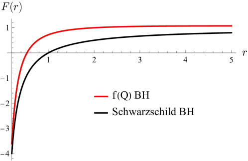
Figure 1: The metric function $F(r)$ of $f(\mathbb{Q})$ BHs and Schwarzschild BHs, where $\alpha=0.2$, $k=10$, and $r_{0}=0.1$ are chosen.

To analyze waveforms, the wave function can be expressed as $\Phi(r,t)=\phi(r)\mathrm{e}^{-\mathrm{i}\omega t}$, where $\omega$ is a complex frequency. The real part of $\omega$ represents the oscillation frequency, while the imaginary part describes the damping rate. It has been shown that the perturbation equations of massless scalar and vector (electromagnetic) fields, governed by the Klein-Gordon equation under the Levi-Civita connection, can be separated [61, 27] into the following form,

$$\left(\partial^{2}_{r^{*}}+\omega^{2}\right)\phi(r^{*})=V_{\mathrm{eff}}\ \phi(r^{*}),$$ (23)

where $r^{*}$ is the tortoise coordinate defined by

$$\frac{\mathrm{d}r^{*}}{\mathrm{d}r}=\frac{1}{F(r)},$$ (24)

and $V_{\mathrm{eff}}$ is the effective potential given by

$$V_{\mathrm{eff}}=F(r)\left[\frac{l(l+1)}{r^{2}}+\frac{1-s^{2}}{r}\frac{\mathrm{d}F(r)}{\mathrm{d}r}\right].$$ (25)

Here, $s=0$ corresponds to the scalar field, $s=1$ describes the electromagnetic field, and $l$ is the orbital angular momentum of the test field.

Figure 2 illustrates the behavior of $V_{\mathrm{eff}}$ as a function of the tortoise coordinate $r^{*}$, where the parameter $\alpha$ is suitably fixed for the comparison to the effective potential of a Schwarzschild BH for reference. The plot shows that $V_{\mathrm{eff}}$ consistently scales upward, and its peak shifts closer to the horizon as the parameter $\alpha$ increases. Notably, this trend is consistent in different types of perturbations. While we provide numerical results for each type of perturbations, our discussion primarily focuses on the scalar perturbation in order to explore the properties of BHs in $f(\mathbb{Q})$ gravity.

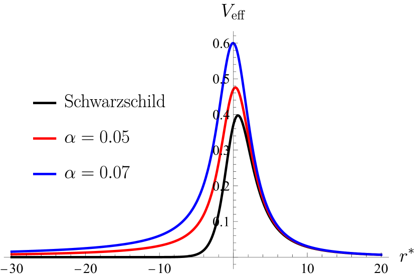
(a) Scalar field perturbation.

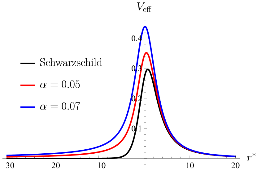
(b) Electromagnetic field perturbation.

Figure 2: The effective potential $V_{\mathrm{eff}}$ as a function of the tortoise coordinate $r^{*}$, where the orbital angular momentum $l$ is fixed to be $1$. Two sets of parameters are chosen for each type of perturbations: Set 1 ($\alpha=0.05$, $k=20$, $r_{0}=0.1$) and set 2 ($\alpha=0.07$, $k=20$, $r_{0}=0.1$). For comparison, $V_{\mathrm{eff}}$ of a Schwarzschild BH is also included.

Moreover, $V_{\mathrm{eff}}$ vanishes at both the spatial infinity ($r^{*}\to\infty$) and the event horizon ($r^{*}\to-\infty$). This behavior contrasts with that observed in $f(\mathbb{T})$ gravity, where $V_{\mathrm{eff}}$ of $f(\mathbb{T})$ approaches a nonzero positive value near the horizon (see Figure 2 in Ref. [27]). Such a difference typically arises in cases where the components of BH metrics, $g_{00}$ and $g_{11}$, do not satisfy the condition: $g_{00}g_{11}=-1$, and thus the zeros of the function $1/g_{11}$ (definition of horizons) are not the zeros of $g_{00}$.

In our case, as described in Eq. (17), the condition $g_{00}g_{11}=-1$ holds, and the zeros of $1/g_{11}$ coincide with those of $g_{00}$. Consequently, no choice of parameters results in a nonzero effective potential near the horizon, as indicated in Eq. (25). However, if we approximate the tortoise coordinates to simplify the calculation of the waveform in the subsequent analysis, we note that this approximation gives the following form when we expand to the second order in $\alpha$,

$$r^{*}=r+\ln(r-1)+\alpha\left[\frac{1}{1-r}+\ln(r-1)\right]+\mathcal{O}(\alpha^{2}).$$ (26)

This leads to two possible deformations of the effective potential, as shown in Fig. 3. These deformations significantly influence the late-time tails of perturbation waveforms during the ringdown phase, as demonstrated in subsequent sections. In other words, the non-vanishing of the effective potential is not limited to specific black hole models discussed in the Ref. [27], but also arises in the approximation of tortoise coordinates. This highlights the need for a rigorous assessment of the validity of such approximations when we analyze perturbation waveforms.

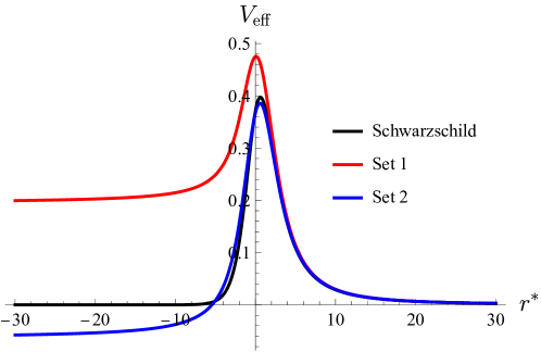
Figure 3: Deformations of the effective potential for the scalar perturbation under two sets of parameters: Set 1 ($\alpha=0.05$, $k=20$, $r_{0}=0.1$) and Set 2 ($\alpha=0.05$, $k=5$, $r_{0}=0.1$).

4 Method and Result

Now we employ the finite difference method to compute the waveform of perturbations and extract the quasinormal frequencies (QNFs) through the nonlinear fitting. Additionally, we apply the WKB approximation to calculate QNFs in a broad range of parameter values.

4.1 Finite difference method

The finite difference method, introduced by Gundlach et al. in 1994 [62], remains widely used due to its simplicity and rigorously established convergence. This method operates in the $u-v$ coordinates, defined as

$$\mathrm{d}u=\mathrm{d}t-\mathrm{d}r^{*},\qquad\mathrm{d}v=\mathrm{d}t+\mathrm{d}r^{*}.$$ (27)

To implement the method, a $u-v$ grid with a uniform spacing $h$ is constructed, see Fig. 4.

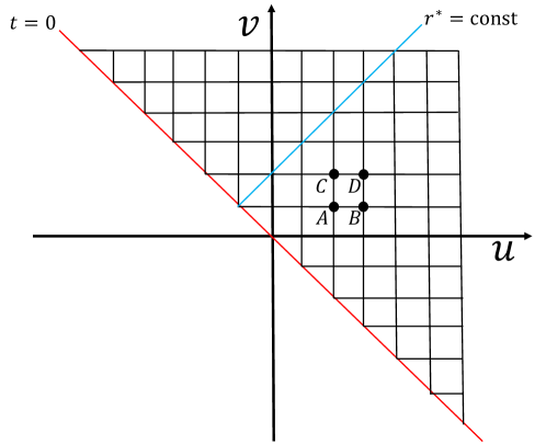
Figure 4: The integration grid is chosen for solving the wave equation. Each grid point corresponds to a value of the wave intensity $\Phi(u,v)$. The points $A$, $B$, $C$ and $D$ illustrate the relative positioning of adjacent points. Initial conditions are assigned along the $t=0$ line, and the time decay behavior for a specific $r^{*}$ is extracted along the $r^{*}=\mathrm{const.}$ line.

The wave equation, given in Eq. (23), is reformulated as

$$\left[4\partial_{u}\partial_{v}+V_{\mathrm{eff}}(u,v)\right]\Phi(u,v)=0,$$ (28)

and is discretized into the form,

$$\Phi(D)=\Phi(B)+\Phi(C)-\Phi(A)-\frac{h^{2}}{8}V_{\mathrm{eff}}(A)\left[\Phi(B)+\Phi(C)\right]+\mathcal{O}\left(h^{4}\right).$$ (29)

This equation gives the basis for numerical integration.

If the initial values are specified along the lower left edge of the integration grid, which stands for $t=0$, Eq. (29) can be used iteratively to compute the values of $\Phi$ across the grid. By transforming back to the $t-r^{*}$ coordinate system, we can obtain the relation between $\Phi(t,r^{*})$ and $t$ for any chosen $r^{*}$.

It is important to note that we need an approximate expression of the tortoise coordinate in the numerical computation of the effective potential. Specifically, an exact expression of $r^{*}$ cannot be directly derived from

$$r^{*}=\int\frac{\mathrm{d}r}{F(r)}.$$ (30)

To address this challenge, we expand the integral near $\alpha=0$ and numerically determine the horizon $r_{\mathrm{H}}$, where $F(r_{\mathrm{H}})=0$. By imposing the boundary condition $r^{*}\to-\infty$ as $r\to r_{\mathrm{H}}$, and retaining the terms up to the first-order correction in $\alpha$, we derive the following expression for the tortoise coordinate,

$$r^{*}=r+\ln(r-r_{\mathrm{H}})+\alpha\left[\frac{1}{r_{\mathrm{H}}-r}+\ln(r-r_{\mathrm{H}})\right].$$ (31)

This approximate formulation will be used in our following calculations.

Figure 5 illustrates the results of exemplary numerical integrations, where $\alpha=0.05$, $k=20$, and $r_{0}=0.1$ are fixed, and $r^{*}$ is held constant, $r^{*}=5$. The scalar field perturbation is performed as a Gaussian wave packet, $\Phi(r^{*})=\exp[-(r^{*}-r^{*}_{c})^{2}/2]$, whose center is at $r^{*}_{c}=2$. The result of the Schwarzschild BH is included for comparison.

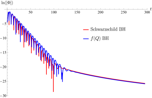
Figure 5: The waveform of scalar field perturbations is shown with parameters $\alpha=0.05$, $k=20$, and $r_{0}=0.1$.

We can see that the waveform of scalar field perturbations around the $f(\mathbb{Q})$ BH is similar to that around the Schwarzschild BH, that is, the three-stage decay process: an initial phase influenced by the perturbation’s type and location, the ringdown period characterized by QNMs, and finally, a late-time tail phase described by a smooth power-law decay (a curve in the logarithmic plot). It is clear that the $f(\mathbb{Q})$ BH demonstrates the comparable early, mid-term, and late behaviors to those in the Schwarzschild BH.

The above phenomenon contrasts with that observed in $f(\mathbb{T})$ gravity for certain solutions (see Fig. 6 in Ref. [27]), where the waveform of the extremely late stage perturbation field still remains oscillating, owing partly to the effective potential $V_{\mathrm{eff}}$ approaching a nonzero value near the horizon in $f(\mathbb{T})$ gravity. This distinction offers a potential observational means to differentiate between $f(\mathbb{Q})$ and $f(\mathbb{T})$ gravity theories.

If the center of Gaussian wave packets is altered, the waveform takes a translational displacement along the direction of time and the onset time of tail phases changes, but the oscillation frequency $\omega$ keeps unchanged, as shown in Fig. 6. This behavior supports the interpretation that the oscillation frequency depends on $V_{\mathrm{eff}}$, but does not on $r_{c}$. QNFs can be extracted in terms of data fitting with a suitable waveform. If the waveform is described in the ringdown phase by

$$\Phi(t)=\mathrm{Re}\sum_{n}A_{n}\mathrm{e}^{-\mathrm{i}[(a_{n}+\mathrm{i}b_{n})t-B_{n}]},$$ (32)

the fitting process can be efficiently performed with the help of the Prony method [42].

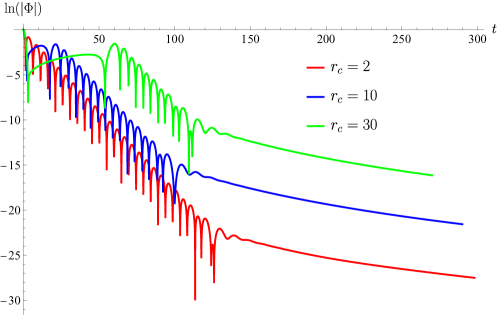
Figure 6: Waveform of scalar field perturbations is shown when the center of perturbation wave packets, $r_{c}$, is varied, where $l=1$, $\alpha=0.05$, $k=20$, and $r_{0}=0.1$ are set. The oscillation frequency is independent of the values of $r_{c}$, but the onset time of tail phases is dependent on them.

Figure 7 illustrates the effects of three key parameters, $\alpha$, $k$, and $r_{0}$, on the waveform of scalar field perturbations. As $\alpha$ increases, representing a greater deviation from GR in terms of the action, the decay rate decreases while the oscillation frequency increases. For $k$, which quantifies deviations from GR at extreme distances where observations are quite possible, an increase leads to higher decay rates and oscillation frequencies. In contrast, $r_{0}$ behaves differently. An increase in $r_{0}$ does not influence the decay rate but causes the tail phase to appear earlier. This is expected, as changes in $r_{0}$ can be interpreted as a rescaling of the black hole’s mass.

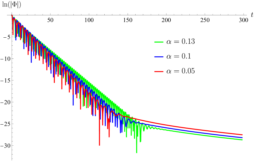
(a)

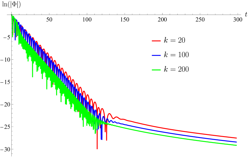
(b)

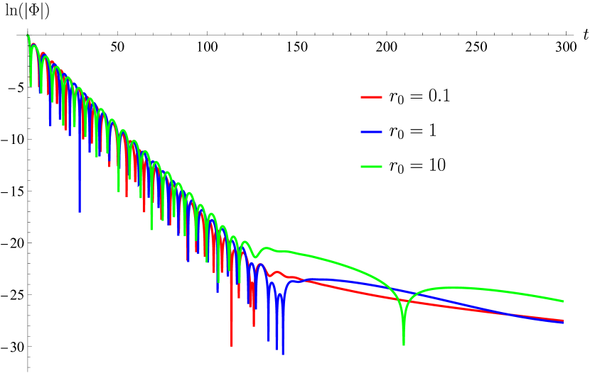
(c)

Figure 7: Waveform of scalar field perturbations under variations in the three parameters, where $l=1$ is fixed for the three cases. Diagram (a) corresponds to a varying $\alpha$ but $k=20$ and $r_{0}=0.1$; diagram (b) corresponds to a varying $k$ but $\alpha=0.05$ and $r_{0}=0.1$; and diagram (c) corresponds to a varying $r_{0}$ but $\alpha=0.05$ and $k=20$.

Remark 2

In order to see that the change of $r_{0}$ can be regarded as a scaling of the mass, we rewrite Eq. (21) in the following form,

$$F(r)=1-\frac{1+\alpha+\alpha^{2}k\ln(r_{0})}{r}+\alpha^{2}k\,\frac{\ln(r)}{r}.$$ (33)

Since the term $1/r$ is related to the significance of mass, any value of $r_{0}$ can be seen as a mass scaling from the case $r_{0}=1$.

Moreover, the tail phase exhibits weaker intensity for larger values of $\alpha$ or $k$. Notably, when any of the three parameters, $\alpha$, $k$, or $r_{0}$, becomes excessively large, exceeding the parameter selection criteria outlined in Sec. 3, the tail phase transitions into a single, sustained oscillation with a low frequency. Beyond these observations, no other significant effects from parameter variations have been identified. This aligns with expectations, as the logarithmic correction to the Schwarzschild metric must remain minimal within the chosen parameter range to avoid contradictions with observational data at extreme distances from the BH. Extreme parameter values are therefore of limited physical relevance. This is consistent with the underlying assumption of a small $\alpha$ in our $f(\mathbb{Q})$ BH solution, which naturally constrains the permissible range of $\alpha$.

4.2 Sixth-order WKB method

The WKB method is widely used in calculations of the QNMs of BHs due to its efficiency and accuracy. Originally developed independently by several researchers in the 1920s for solving wave equations in quantum mechanics, the method was first applied to QNM calculations by Schutz et al. in the 1980s [63], see also Ref. [55], owing to the similarity between the perturbation equation (Eq. (23)) and the Schrödinger equation.

To enhance its accuracy, higher-order WKB approximations have been developed [64, 65], where one advantage is to replace the traditional Taylor expansion with the Padé approximation, see also Ref. [61]. It is worth noting that the WKB method is generally more accurate for a higher value of $l$ [27].

Figures 8, 9, and 10 depict the relationship between $\omega$ (real and imaginary parts) and the three parameters $\alpha$, $k$, and $r_{0}$, respectively, for a varying angular momentum number $l$.

For spherically symmetric BHs in $f(\mathbb{Q})$ gravity, the real and imaginary parts of the QNM frequency $\omega$ exhibit a significant, nonlinear dependence on the parameter $\alpha$, see Fig. 8. The both parts reach their minimum absolute values around $\alpha$ = 0.5 and increase as $\alpha$ diverges from this value. A bigger $\alpha$ corresponds to a higher oscillation frequency and a faster decay rate. Consequently, the relationship between the real $\omega_{\mathrm{Re}}$ and imaginary $\omega_{\mathrm{Im}}$ parts becomes nonlinear since neither $\omega_{\mathrm{Re}}$ nor $\omega_{\mathrm{Im}}$ varies monotonically. This suggests that changes in $\alpha$ can drive the black hole to transition between different thermodynamic phases. The critical points of these phase transitions correspond to the extremal values of the real and imaginary components.

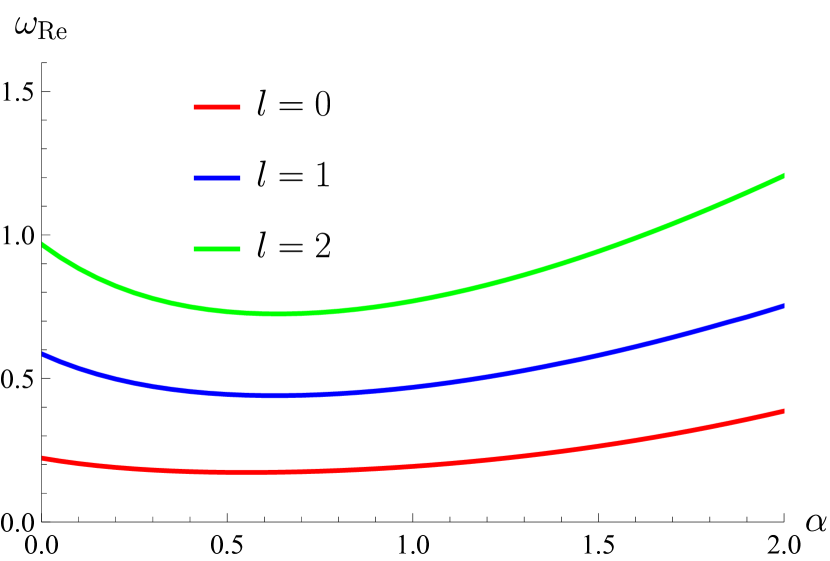
(a) The real part.

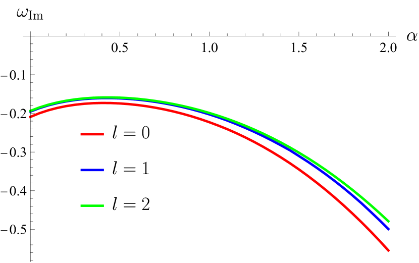
(b) The imaginary part.

Figure 8: The relationship of QNMs with respect to $\alpha$ in $f(\mathbb{Q})$ gravity for a varying $l$, where $k=1$ and $r_{0}=1$ are set. The calculations are made by the sixth-order WKB method, together with the Padé approximation, under a massless scalar field perturbation.

Figure 9 demonstrates that the real and imaginary parts exhibit an approximately linear dependence on $k$, with their absolute values increasing as $k$ grows. That is, a bigger $k$ results in a higher oscillation frequency and a faster decay rate.

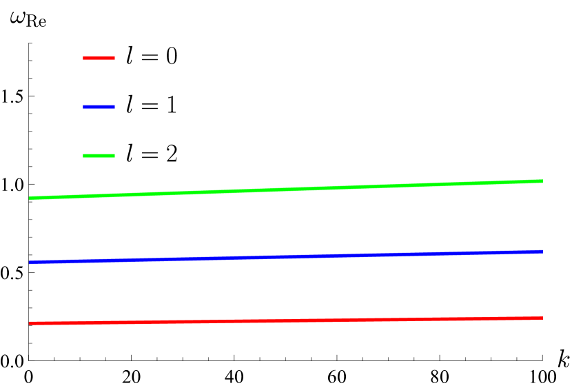
(a) The real part.

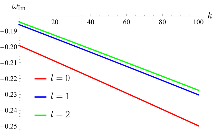
(b) The imaginary part.

Figure 9: The relationship of QNMs with respect to $k$ in $f(\mathbb{Q})$ gravity for a varying $l$, where $\alpha=0.05$ and $r_{0}=1$ are set. The calculations are made by the sixth-order WKB method, together with the Padé approximation, under a massless scalar field perturbation.

The impact of $r_{0}$ is not further analyzed, see Fig. 10, since any $r_{0}$ can effectively be redefined as $r_{0}\equiv 1$ with an additional term proportional to $1/r$. This redefinition allows $r_{0}$ to be treated purely as a mass correction term, see the above Remark 2.

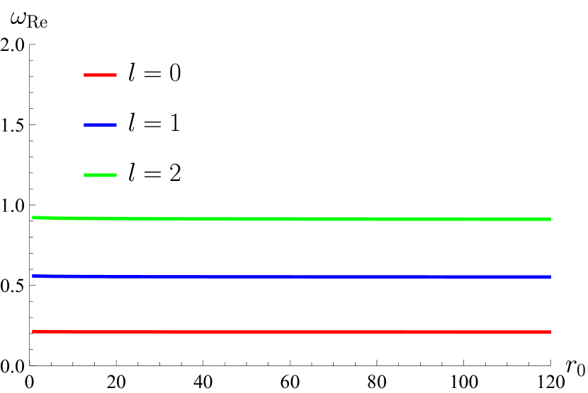
(a) The real part.

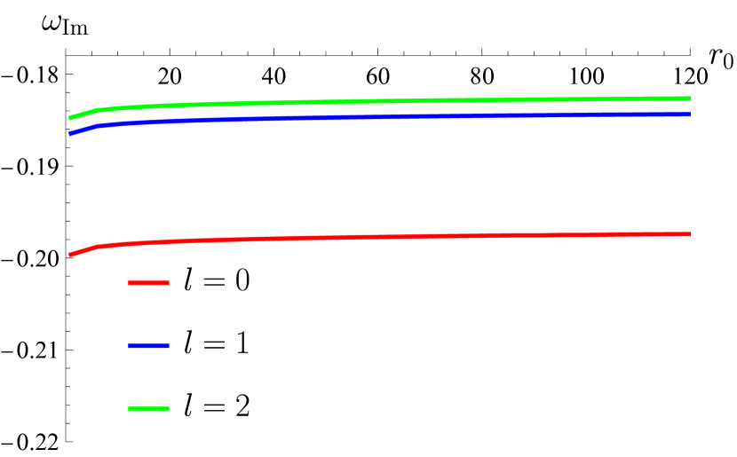
(b) The imaginary part.

Figure 10: The relationship of QNMs with respect to $r_{0}$ in $f(\mathbb{Q})$ gravity for a varying $l$, where $\alpha=0.05$ and $k=1$ are set. The calculations are made by the sixth-order WKB method, together with the Padé approximation, under a massless scalar field perturbation.

The detailed numerical results, for the relationship of QNMs with respect to $\alpha$ in $f(\mathbb{Q})$ gravity, see Fig. 8, are presented in Table 1 for scalar field perturbations and Table 2 for vector field perturbations, respectively. Since our primary focus is on the effects of deviations from GR, primarily characterized by $\alpha$, we present the data with $\alpha$ and $l$ as the variables.

$\alpha$	$l$	$n=0$		$n=1$		$n=2$
		$\omega_{\mathrm{Re}}$	$\omega_{\mathrm{Im}}$	$\omega_{\mathrm{Re}}$	$\omega_{\mathrm{Im}}$	$\omega_{\mathrm{Re}}$	$\omega_{\mathrm{Im}}$
0	0	0.222620	-0.209111	0.175050	-0.710126	0.156048	-1.22490
	1	0.585861	-0.195322	0.528913	-0.613014	0.457699	-1.08433
	2	0.967287	-0.193518	0.927692	-0.591251	0.860659	-1.01733
0.01	0	0.220429	-0.207065	0.173323	-0.703167	0.154479	-1.21292
	1	0.580085	-0.193406	0.523691	-0.607004	0.453175	-1.07371
	2	0.957750	-0.191620	0.918540	-0.585452	0.852160	-1.00735
0.02	0	0.218304	-0.205088	0.171657	-0.696493	0.153056	-1.20136
	1	0.574473	-0.191563	0.518605	-0.601230	0.448753	-1.06351
	2	0.948481	-0.189793	0.909636	-0.579875	0.843875	-0.997769
0.05	0	0.212324	-0.199633	0.166947	-0.678074	0.148942	-1.16952
	1	0.558586	-0.186453	0.504134	-0.585252	0.436101	-1.03536
	2	0.922233	-0.184726	0.884364	-0.564417	0.820268	-0.971238
0.1	0	0.203579	-0.191982	0.160021	-0.652268	0.142708	-1.12498
	1	0.535095	-0.179219	0.482515	-0.562740	0.416983	-0.995880
	2	0.883392	-0.177542	0.846797	-0.542545	0.784901	-0.933827
0.2	0	0.190084	-0.181137	0.149307	-0.616157	0.133293	-1.06238
	1	0.497991	-0.168834	0.447648	-0.530807	0.385478	-0.940565
	2	0.821945	-0.167199	0.786809	-0.511208	0.727535	-0.880661
0.5	0	0.172906	-0.174245	0.136059	-0.595802	0.122303	-1.02535
	1	0.444467	-0.161095	0.392410	-0.510205	0.331746	-0.910283
	2	0.732588	-0.159220	0.695599	-0.488351	0.634230	-0.845612
1	0	0.193755	-0.222795	0.157846	-0.764374	0.145115	-1.30943
	1	0.469260	-0.202566	0.393509	-0.654413	0.322865	-1.18494
	2	0.769767	-0.198892	0.712150	-0.616491	0.622852	-1.08434
2	0	0.386461	-0.554405	0.325143	-1.85510	0.334315	-3.18142
	1	0.753196	-0.499051	0.556084	-1.70630	0.480756	-3.02778
	2	1.20638	-0.478970	1.01556	-1.54688	0.824896	-2.82105

Table 1: QNMs for scalar field perturbations, where $k=1$ and $r_{0}=1$ are fixed.

$\alpha$	$l$	$n=0$		$n=1$		$n=2$
		$\omega_{\mathrm{Re}}$	$\omega_{\mathrm{Im}}$	$\omega_{\mathrm{Re}}$	$\omega_{\mathrm{Im}}$	$\omega_{\mathrm{Re}}$	$\omega_{\mathrm{Im}}$
0	0	0.496503	-0.184969	0.428543	-0.588209	0.346032	-1.05977
	1	0.915190	-0.190010	0.873066	-0.581454	0.801716	-1.00339
	2	1.31380	-0.191233	1.28347	-0.579461	1.22756	-0.984115
0.01	0	0.491602	-0.183154	0.424303	-0.582439	0.342598	-1.04939
	1	0.906163	-0.188145	0.864449	-0.575750	0.793794	-0.993551
	2	1.30084	-0.189356	1.27081	-0.573776	1.21545	-0.974462
0.02	0	0.486829	-0.181404	0.420156	-0.576889	0.339218	-1.03941
	1	0.897383	-0.186350	0.856057	-0.570262	0.786060	-0.984092
	2	1.28824	-0.187550	1.25849	-0.568306	1.20364	-0.965179
0.05	0	0.473255	-0.176539	0.408260	-0.561496	0.329405	-1.01185
	1	0.872485	-0.181366	0.832195	-0.555034	0.763965	-0.957891
	2	1.25254	-0.182537	1.22354	-0.553127	1.17006	-0.939441
0.1	0	0.452992	-0.169604	0.390195	-0.539696	0.314156	-0.973139
	1	0.835526	-0.174284	0.796587	-0.533446	0.730682	-0.920881
	2	1.19962	-0.175419	1.17158	-0.531600	1.11991	-0.90301
0.2	0	0.420362	-0.159482	0.360104	-0.508376	0.287673	-0.918624
	1	0.776690	-0.164032	0.739284	-0.502357	0.676113	-0.868067
	2	1.11559	-0.165133	1.08865	-0.500574	1.03905	-0.850773
0.5	0	0.368757	-0.150491	0.305531	-0.484782	0.232783	-0.887315
	1	0.688460	-0.155641	0.648948	-0.478314	0.583125	-0.831339
	2	0.991238	-0.156876	0.962735	-0.476367	0.910587	-0.812247
1	0	0.367154	-0.182131	0.269478	-0.608092	0.173153	-1.15792
	1	0.710222	-0.192072	0.647785	-0.597223	0.549026	-1.05740
	2	1.03086	-0.194393	0.985534	-0.593752	0.904682	-1.02320
2	0	0.442449	-0.371429	0.107266	-1.47556	0.265593	0.706881
	1	1.01997	-0.436967	0.788724	-1.43460	0.503217	-2.71663
	2	1.53931	-0.451478	1.36606	-1.41679	1.09612	-2.54715

Table 2: QNMs for vector field perturbations, where $k=1$ and $r_{0}=1$ are fixed.

5 Comparison and discussion

In this section, we begin by comparing the QNMs of BHs in $f(\mathbb{Q})$ gravity with those in $f(\mathbb{T})$ gravity. We then examine the impact of the non-vanishing behavior of the effective potential near the horizon in $f(\mathbb{Q})$, focusing on how this phenomenon influences the tail behavior of perturbation waveforms.

5.1 Comparison with $f(\mathbb{T})$ gravity

We mainly focus on the difference between QNMs in $f(\mathbb{Q})$ gravity and those in $f(\mathbb{T})$ gravity, the two gravity theories are expressed in the form of the series expansion and preserved to a quadratic term, that is, $f(\mathbb{Q})=\mathbb{Q}+\alpha\mathbb{Q}^{2}$ and $f(\mathbb{T})=\mathbb{T}+\beta\mathbb{T}^{2}$. The reason that we ignore $f(\mathbb{R})$ gravity is $f(\mathbb{R})=\mathbb{R}+\gamma\mathbb{R}^{2}$ only gives a correction term which is proportional to ${1}/{r}$ in the metric function, which can be treated as a correction of mass. Here $\beta$ and $\gamma$ are perturbative parameters. Thus, $f(\mathbb{R})$ gravity cannot give any nontrivial result beyond GR, but just provides [42] the effect of mass on QNMs. The following results on $f(\mathbb{T})$ gravity come from Ref. [27].

The QNM spectra for both $f(\mathbb{Q})$ gravity and $f(\mathbb{T})$ gravity are presented in Fig. 11. In $f(\mathbb{Q})$ gravity, $\omega_{\mathrm{Re}}$ exhibits a minimum with respect to $\omega_{\mathrm{Im}}$, and both $\omega_{\mathrm{Re}}$ and $\omega_{\mathrm{Im}}$ are double-valued relative to each other. This characteristic is also observed in $f(\mathbb{T})$ gravity. For the two ansätze in $f(\mathbb{T})$ gravity, the spectrum of ansatz 1 resembles that of $f(\mathbb{Q})$ gravity, while ansatz $2$ shows a maximum in $\omega_{\mathrm{Re}}$.

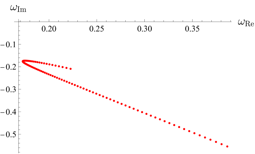
(a) $f(\mathbb{Q})$ gravity.

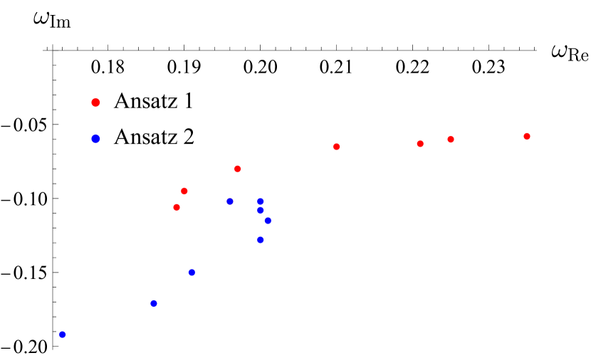
(b) $f(\mathbb{T})$ gravity.

Figure 11: The spectra of QNMs in both $f(\mathbb{Q})$ gravity and $f(\mathbb{T})$ gravity, where the perturbative parameters $\alpha$ and $\beta$ vary from $0$ to $2$, respectively, under a massless scalar field perturbation. Diagram (a) for $f(\mathbb{Q})$ gravity, where $l=0$, $n=0$, $k=1$, and $r_{0}=1$ are fixed, is based on the data in Table 1. Diagram (b) is from Table 1 of Ref. [27] for $f(\mathbb{T})$ gravity, where Ansatz 1 and Ansatz 2 are corresponding to the two families of solutions.

Notably, the oscillatory decay in the late-stage waveform of ansatz $1$ suggests that it may be possible to distinguish between these three solutions observationally. The distinctive QNM spectrum features in $f(\mathbb{Q})$ and $f(\mathbb{T})$ gravity are reminiscent of patterns associated with phase transitions, such as those seen in Reissner–Nordström black holes [66]. Specifically, the turning point in Fig. 11 may correspond to the Davies point, which marks second-order phase transitions [67]. Further investigation from a thermodynamic perspective is required to confirm this connection, which we plan to address in our future work.

In contrast to $f(\mathbb{Q})$ gravity, the QNMs of the two families of spherically symmetric BH solutions in $f(\mathbb{T})$ gravity appear less sensitive to $\alpha$, though some correlations remain evident. As shown in Fig. 7 of Ref. [27], the absolute values of the real and imaginary parts of the QNMs in $f(\mathbb{T})$ gravity decrease as $\alpha$ increases, resulting in lower oscillation frequencies and slower decay rates.

It is obvious that, for the same $M$ and $l$, the sensitivity of QNMs to $\alpha$ is significantly more pronounced in $f(\mathbb{Q})$ gravity, with the relationship between the real and imaginary parts of the QNMs exhibiting an opposite trend compared to $f(\mathbb{T})$ gravity. This distinction provides a potential observational means to differentiate between the two theories.

Furthermore, it is worth noting that the first family of solutions in Ref. [27] closely differs from the solutions in $f(\mathbb{Q})$ gravity, where the former is characterized by a non-zero effective potential near the horizon. In contrast, the second family’s effective potential approaches zero near the horizon, leading to a slow power-law decay tail similar to that observed in $f(\mathbb{Q})$ gravity.

For fixed $k=1$ and $r_{0}=1$, the parameter $r_{0}$ remains inside the event horizon, see Fig. 12. We attribute this behavior to the influence of the $\alpha^{2}$ term, which plays a critical role in shaping the system’s dynamics.

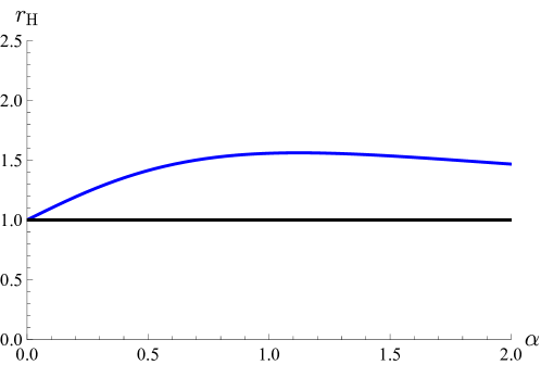
Figure 12: The relationship between the horizon radius and $\alpha$ in $f(\mathbb{Q})$ gravity (blue curve), where $l=0$, $n=0$, $k=1$, and $r_{0}=1$ are fixed. Note that $r_{0}$ (black line) always remains inside the horizon ($r_{\rm H}\geq 1$).

Moreover, when the angular momentum quantum number $l$ increases, the real part of QNMs becomes increasingly sensitive to $\alpha$, while the imaginary part does conversely. This highlights the intricate dependence of QNMs on both $\alpha$ and $l$, emphasizing their significance in determining the dynamics of BHs in $f(\mathbb{Q})$ gravity.

5.2 Discussion on the non-zero effective potential near horizons

At the end of Sec. 3, we mentioned the non-zero behavior of the effective potential near the horizon, attributed to the approximation of the tortoise coordinate, see Fig. 3. The effective potential in the two sets of parameters can take either positive or negative values, significantly influencing the tail behavior of waveforms. Similar effects have been observed in other theories, such as $f(\mathbb{T})$ gravity, as discussed in Ref. [27]. Such non-zero effective potentials near the horizon commonly occur in spherically symmetric black holes with the algebraic property $[1,1(11)]$, where the metric components $g_{00}$ and $1/g_{11}$ exhibit distinct roots.

In the case that the effective potential near the horizon ($V_{\rm H}$) is positive, see Fig. 13,

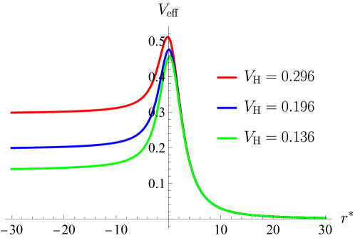
Figure 13: Effective potential with respect to the tortoise coordinate, where the asymptotic values near horizons, $V_{\rm H}$, are positive.

the waveform tails display a unique oscillatory decay, see Fig. 14,

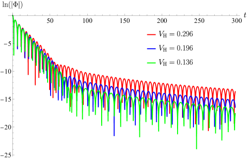
Figure 14: Waveform of scalar field perturbations for positive asymptotic values of effective potentials near horizons.

which differs from the purely decaying tails shown in Figs. 6 and 7. In particular, Fig. 14 shows that a higher $V_{\mathrm{H}}$ causes a higher intensity and a greater frequency in the oscillatory decay of the tail period.

Figure 15: Effective potential which has a negative asymptotic value at the horizon. Here we fix $\alpha=0.1$, $k=10$, $r_{0}=1$, and $l=1$.

In the case that the effective potential near the horizon is negative, the approach used for the positive case leads to a divergent waveform tail. For instance, when we set $\alpha=0.1$, $k=10$, $r_{0}=1$, and $l=1$, the effective potential exhibits the behavior shown in Fig. 15, where the potential approaches a negative value as $r^{*}\to-\infty$. We then apply the finite difference method to analyze the time-domain behavior of the perturbation equation, and give the results displayed in Fig. 16, that is, after an initial delay, positively correlated with the distance from the horizon of black holes, the perturbation fields grow exponentially. This behavior may be compared with that of the Schrödinger-like solution, $\Phi(r,t)=\phi(r)\exp\left(-{\mathrm{i}}Et/{\hbar}\right)$, where $E$ is complex. If the imaginary part of $E$ is positive (corresponding to a negative potential), the evolution of time turns out to be divergent, leading to an unstable state.

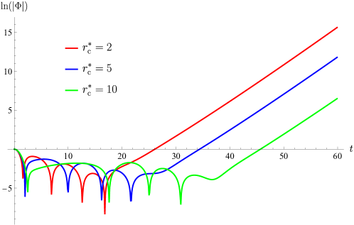
Figure 16: Waveform of perturbation fields for negative asymptotic values of effective potentials near horizons, where the tails grow exponentially.

The above divergent tail is clearly unacceptable because it means that the perturbation field carries an infinite energy. Here we propose three possible interpretations to address it. The first is that any parameter choice resulting in a negative effective potential is inherently unphysical or invalid. It provides a straightforward resolution and imposes stricter constraints on parameter selections in modified gravity theories. The second interpretation is to accept the phenomenon by considering that the test field could draw energy from a black hole, leading to a reduction in the black hole’s ADM mass. In some cases, this process might allow the black hole to transition into a stable phase, characterized by a non-negative effective potential, after which the test field would begin to decay again. Under this view, such parameter choices would represent unstable but not entirely prohibited configurations. However, for other parameter choices, where the black hole’s mass could decrease indefinitely (potentially exposing a naked singularity), these configurations would still be deemed unphysical. The third interpretation suggests that the effective potential should instead be considered in terms of its absolute value. While it offers a different perspective, its validity requires further investigation. The most appropriate resolution for this phenomenon remains an open question. Since this issue lies beyond the primary scope of this work, we defer its detailed discussion to future studies.

6 Conclusion

In this work, we analyze the QNMs of static and spherically symmetric BHs in $f(\mathbb{Q})$ gravity under a massless scalar and electromagnetic field perturbations. We consider a quadratic correction of $\mathbb{Q}$, $f(\mathbb{Q})=\mathbb{Q}+\alpha\mathbb{Q}^{2}$, which serves as a reasonable approximation for any series expansion of $f(\mathbb{Q})$. To simplify the free parameters, we fix $M=1/2$, which means that the mass primarily acts as a scaling factor for the QNM frequencies $\omega$.

By using the tortoise coordinate, we reformulate the general perturbation equations into a Schrödinger-like form, enabling QNM calculations via the finite difference and WKB methods. We extract the effective potentials governing wave evolution, which universally approach zero at infinity and reach a maximum around $r^{*}=3/2$. Notably, regardless of the parameter values, the effective potential near the horizon always vanishes. This behavior contrasts with that of $f(\mathbb{T})$ gravity [27], where one solution yields a positive effective potential near the horizon, leading to oscillatory power-law decay at fixed frequencies in the wave tail, a clear observational distinction between $f(\mathbb{T})$ and $f(\mathbb{Q})$.

We calculate the QNMs with the finite difference method and the 6th-order WKB Padé approximation, give the time evolution of perturbation waves, and analyze the relationships between QNM frequencies and the parameters, like the angular momentum $l$, the correction coefficient $\alpha$, the integral constant $k$, and $r_{0}$, respectively. In particular, we emphasize the physical significance of these parameters. Our results show that $f(\mathbb{Q})$ gravity introduces QNM features distinct from those of GR, with a strong dependence on the correction coefficient and other parameters. A notable feature of QNMs in $f(\mathbb{Q})$ gravity is the “closed” spectrum, where the real and imaginary parts are double-valued with respect to each other. This means that the different decay rates may be observed for the same oscillation frequency, and vice versa, which is an important observational signature of $f(\mathbb{Q})$ gravity.

Our comparisons to $f(\mathbb{T})$ gravity with a quadratic correction reveal that the QNMs in $f(\mathbb{Q})$ gravity are more sensitive to parameter changes. Moreover, the relationship between the QNMs and the perturbative parameter in $f(\mathbb{Q})$ gravity is opposite to that in $f(\mathbb{T})$ gravity. These differences may offer a promising basis for distinguishing the two theories through observations. It is worth mentioning that the first family of solutions in $f(\mathbb{T})$ gravity has a different waveform from that in $f(\mathbb{Q})$ gravity, while the second family of solutions in $f(\mathbb{T})$ gravity has the different spectrum from that in $f(\mathbb{Q})$ gravity. It offers a practical way to distinguish them under observation.

We also make a brief analysis of the influence of effective potentials with non-zero values near horizons in $f(\mathbb{Q})$ gravity, which leads to a unique oscillatory decay of the third period or an abnormal exponential increase, depending on whether the value is positive or negative. Moreover, real black holes are often rotating, making it important to construct on-shell rotating black hole solutions in both $f(\mathbb{T})$ and $f(\mathbb{Q})$ frameworks and to analyze their spectra [68]. This aspect will be a focus of our future research.

It is worthy to notice that we use the Klein-Golden equation in the Levi-Civita connection when we derive the perturbation equation. This is a widely accepted convention in the study of quasinormal modes of BHs under modified gravity [27, 55, 56]. Although the Levi-Civita connection is consistent with the coincident gauge in our consideration, it is an approximation in general since the connection under a non-Riemannian geometry may differ from the Levi-Civita connection and may have a relationship with parameters in different models. This issue becomes particularly significant when the connection used to solve black hole solutions differs from the one employed for test-field perturbations. Such inconsistency can lead to discrepancies in the analysis. Therefore, it is a critical challenge to establish a self-consistent and unified connection for studying the QNMs of test-field perturbations.

In summary, we provide a comprehensive analysis of QNMs in static and spherically symmetric BHs under the framework of $f(\mathbb{Q})$ gravity and highlight several key differences from $f(\mathbb{T})$ gravity theory. Our findings offer a theoretical foundation for evaluating the validity of modified gravity theories and contribute valuable insights into investigating QNMs in alternative theories of gravity. Future work may focus on the QNM properties of rotating BHs in $f(\mathbb{Q})$ gravity.

References

- [1] A. Einstein, “The Field Equations of Gravitation,” Sitzungsber. Preuss. Akad. Wiss. Berlin (Math. Phys. ) 1915 (1915) 844–847.
- [2] Supernova Search Team Collaboration, A. G. Riess et al., “Observational evidence from supernovae for an accelerating universe and a cosmological constant,” Astron. J. 116 (1998) 1009–1038, arXiv:astro-ph/9805201.
- [3] F. Niedermann and M. S. Sloth, “New early dark energy,” Phys. Rev. D 103 no. 4, (2021) L041303, arXiv:1910.10739 [astro-ph.CO].
- [4] E. O. Colgáin, M. M. Sheikh-Jabbari, and L. Yin, “Can dark energy be dynamical?,” Phys. Rev. D 104 no. 2, (2021) 023510, arXiv:2104.01930 [astro-ph.CO].
- [5] S. Nojiri, S. D. Odintsov, and T. Paul, “Barrow entropic dark energy: A member of generalized holographic dark energy family,” Phys. Lett. B 825 (2022) 136844, arXiv:2112.10159 [gr-qc].
- [6] R. G. Landim, “Fractional dark energy,” Phys. Rev. D 103 no. 8, (2021) 083511, arXiv:2101.05072 [astro-ph.CO].
- [7] T. P. Sotiriou and V. Faraoni, “f(R) Theories Of Gravity,” Rev. Mod. Phys. 82 (2010) 451–497, arXiv:0805.1726 [gr-qc].
- [8] S. Nojiri, S. D. Odintsov, and V. K. Oikonomou, “Modified Gravity Theories on a Nutshell: Inflation, Bounce and Late-time Evolution,” Phys. Rept. 692 (2017) 1–104, arXiv:1705.11098 [gr-qc].
- [9] N. Frusciante and L. Perenon, “Effective field theory of dark energy: A review,” Phys. Rept. 857 (2020) 1–63, arXiv:1907.03150 [astro-ph.CO].
- [10] V. K. Oikonomou, “Unifying inflation with early and late dark energy epochs in axion gravity,” Phys. Rev. D 103 no. 4, (2021) 044036, arXiv:2012.00586 [astro-ph.CO].
- [11] R. Solanki, A. De, and P. K. Sahoo, “Complete dark energy scenario in f(Q) gravity,” Phys. Dark Univ. 36 (2022) 100996, arXiv:2203.03370 [gr-qc].
- [12] H. Weyl, Space, time, matter: Lectures on general relativity. (In German). Springer Berlin, Heidelberg, 1919.
- [13] R. Utiyama and B. S. DeWitt, “Renormalization of a classical gravitational field interacting with quantized matter fields,” J. Math. Phys. 3 (1962) 608–618.
- [14] CANTATA Collaboration, Y. Akrami et al., Modified Gravity and Cosmology. An Update by the CANTATA Network. Springer, 2021. arXiv:2105.12582 [gr-qc].
- [15] C. M. Reyes and M. Schreck, “Modified-gravity theories with nondynamical background fields,” Phys. Rev. D 106 no. 4, (2022) 044050, arXiv:2202.11881 [hep-th].
- [16] S. Shankaranarayanan and J. P. Johnson, “Modified theories of gravity: Why, how and what?,” Gen. Rel. Grav. 54 no. 5, (2022) 44, arXiv:2204.06533 [gr-qc].
- [17] J. K. Singh, H. Balhara, K. Bamba, and J. Jena, “Bouncing cosmology in modified gravity with higher-order curvature terms,” JHEP 03 (2023) 191, arXiv:2206.12423 [gr-qc]. [Erratum: JHEP 04, 049 (2023)].
- [18] A. H. Guth, “The Inflationary Universe: A Possible Solution to the Horizon and Flatness Problems,” Phys. Rev. D 23 (1981) 347–356.
- [19] P. Creminelli and F. Vernizzi, “Dark Energy after GW170817 and GRB170817A,” Phys. Rev. Lett. 119 no. 25, (2017) 251302, arXiv:1710.05877 [astro-ph.CO].
- [20] M. Braglia, M. Ballardini, F. Finelli, and K. Koyama, “Early modified gravity in light of the tension and LSS data,” Phys. Rev. D 103 no. 4, (2021) 043528, arXiv:2011.12934 [astro-ph.CO].
- [21] T. Adi and E. D. Kovetz, “Can conformally coupled modified gravity solve the Hubble tension?,” Phys. Rev. D 103 no. 2, (2021) 023530, arXiv:2011.13853 [astro-ph.CO].
- [22] A. A. Starobinsky, “A New Type of Isotropic Cosmological Models Without Singularity,” Phys. Lett. B 91 (1980) 99–102.
- [23] J. Beltrán Jiménez, L. Heisenberg, and T. Koivisto, “Coincident General Relativity,” Phys. Rev. D 98 no. 4, (2018) 044048, arXiv:1710.03116 [gr-qc].
- [24] S. Bahamonde, K. F. Dialektopoulos, C. Escamilla-Rivera, G. Farrugia, V. Gakis, M. Hendry, M. Hohmann, J. Levi Said, J. Mifsud, and E. Di Valentino, “Teleparallel gravity: from theory to cosmology,” Rept. Prog. Phys. 86 no. 2, (2023) 026901, arXiv:2106.13793 [gr-qc].
- [25] L. Heisenberg, “Review on f(Q) gravity,” Phys. Rept. 1066 (2024) 1–78, arXiv:2309.15958 [gr-qc].
- [26] J. Beltrán Jiménez, L. Heisenberg, T. S. Koivisto, and S. Pekar, “Cosmology in geometry,” Phys. Rev. D 101 no. 10, (2020) 103507, arXiv:1906.10027 [gr-qc].
- [27] Y. Zhao, X. Ren, A. Ilyas, E. N. Saridakis, and Y.-F. Cai, “Quasinormal modes of black holes in f(T) gravity,” JCAP 10 (2022) 087, arXiv:2204.11169 [gr-qc].
- [28] N. Dimakis, P. A. Terzis, T. Christodoulakis, and A. Paliathanasis, “Static, spherically symmetric solutions in -gravity and in nonmetricity scalar-tensor theory,” arXiv:2410.04513 [gr-qc].
- [29] A. Golovnev, “Introduction to teleparallel gravities,” in 9th Mathematical Physics Meeting: Summer School and Conference on Modern Mathematical Physics. 1, 2018. arXiv:1801.06929 [gr-qc].
- [30] S. Capozziello, V. De Falco, and C. Ferrara, “Comparing equivalent gravities: common features and differences,” Eur. Phys. J. C 82 no. 10, (2022) 865, arXiv:2208.03011 [gr-qc].
- [31] S. Capozziello, V. De Falco, and C. Ferrara, “The role of the boundary term in f(Q, B) symmetric teleparallel gravity,” Eur. Phys. J. C 83 no. 10, (2023) 915, arXiv:2307.13280 [gr-qc].
- [32] J. Beltrán Jiménez, A. Golovnev, T. Koivisto, and H. Veermäe, “Minkowski space in gravity,” Phys. Rev. D 103 no. 2, (2021) 024054, arXiv:2004.07536 [gr-qc].
- [33] J. Beltrán Jiménez and T. S. Koivisto, “Accidental gauge symmetries of Minkowski spacetime in Teleparallel theories,” Universe 7 no. 5, (2021) 143, arXiv:2104.05566 [gr-qc].
- [34] D. A. Gomes, J. Beltrán Jiménez, A. J. Cano, and T. S. Koivisto, “Pathological Character of Modifications to Coincident General Relativity: Cosmological Strong Coupling and Ghosts in f(Q) Theories,” Phys. Rev. Lett. 132 no. 14, (2024) 141401, arXiv:2311.04201 [gr-qc].
- [35] A. G. Bello-Morales, J. Beltrán Jiménez, A. Jiménez Cano, T. S. Koivisto, and A. L. Maroto, “A class of ghost-free theories in symmetric teleparallel geometry,” JHEP 12 (2024) 146, arXiv:2406.19355 [gr-qc].
- [36] S. Chandrasekhar, The mathematical theory of black holes. Springer Netherlands, Dordrecht, 1984.
- [37] V. P. Frolov and I. D. Novikov, eds., Black hole physics: Basic concepts and new developments. Springer Dordrecht, 1998.
- [38] R.-G. Cai, Z. Cao, Z.-K. Guo, S.-J. Wang, and T. Yang, “The Gravitational-Wave Physics,” Natl. Sci. Rev. 4 no. 5, (2017) 687–706, arXiv:1703.00187 [gr-qc].
- [39] M. Hohmann, C. Pfeifer, J. Levi Said, and U. Ualikhanova, “Propagation of gravitational waves in symmetric teleparallel gravity theories,” Phys. Rev. D 99 no. 2, (2019) 024009, arXiv:1808.02894 [gr-qc].
- [40] H.-P. Nollert, “TOPICAL REVIEW: Quasinormal modes: the characteristic ‘sound’ of black holes and neutron stars,” Class. Quant. Grav. 16 (1999) R159–R216.
- [41] E. Berti, V. Cardoso, and A. O. Starinets, “Quasinormal modes of black holes and black branes,” Class. Quant. Grav. 26 (2009) 163001, arXiv:0905.2975 [gr-qc].
- [42] R. A. Konoplya and A. Zhidenko, “Quasinormal modes of black holes: From astrophysics to string theory,” Rev. Mod. Phys. 83 (2011) 793–836, arXiv:1102.4014 [gr-qc].
- [43] M. Maggiore, Gravitational Waves. Vol. 2: Astrophysics and Cosmology. Oxford University Press, 3, 2018.
- [44] Z. Zhu, S.-J. Zhang, C. E. Pellicer, B. Wang, and E. Abdalla, “Stability of Reissner-Nordström black hole in de Sitter background under charged scalar perturbation,” Phys. Rev. D 90 no. 4, (2014) 044042, arXiv:1405.4931 [hep-th]. [Addendum: Phys.Rev.D 90, 049904 (2014)].
- [45] S. Bhattacharyya and S. Shankaranarayanan, “Quasinormal modes as a distinguisher between general relativity and f(R) gravity,” Phys. Rev. D 96 no. 6, (2017) 064044, arXiv:1704.07044 [gr-qc].
- [46] Y. Guo and Y.-G. Miao, “Scalar quasinormal modes of black holes in Einstein-Yang-Mills gravity,” Phys. Rev. D 102 no. 6, (2020) 064049, arXiv:2005.07524 [hep-th].
- [47] T. Zhu, W. Zhao, J.-M. Yan, Y.-Z. Wang, C. Gong, and A. Wang, “Constraints on parity and Lorentz violations in gravity from GWTC-3 through a parametrization of modified gravitational wave propagations,” Phys. Rev. D 110 no. 6, (2024) 064044, arXiv:2304.09025 [gr-qc].
- [48] Z.-W. Xia, H. Yang, and Y.-G. Miao, “Scalar fields around a rotating loop quantum gravity black hole: waveform, quasi-normal modes and superradiance,” Class. Quant. Grav. 41 no. 16, (2024) 165010, arXiv:2310.00253 [gr-qc].
- [49] H. Yang, Z.-W. Xia, and Y.-G. Miao, “Echoes and quasi-normal modes of perturbations around Schwarzchild traversable wormholes,” arXiv:2406.00377 [gr-qc].
- [50] A. Aragón, P. A. González, E. Papantonopoulos, and Y. Vásquez, “Quasinormal modes and their anomalous behavior for black holes in gravity,” Eur. Phys. J. C 81 no. 5, (2021) 407, arXiv:2005.11179 [gr-qc].
- [51] Y. Younesizadeh, A. H. Ahmed, A. A. Ahmad, Y. Younesizadeh, and M. Ebrahimkhas, “New class of solutions in f(R)-gravity’s rainbow and f(R)-gravity: Exact solutions+thermodynamics+quasinormal modes,” Nucl. Phys. B 971 (2021) 115376.
- [52] A. Ovgün and K. Jusufi, “Quasinormal Modes and Greybody Factors of gravity minimally coupled to a cloud of strings in Dimensions,” Annals Phys. 395 (2018) 138–151, arXiv:1801.02555 [gr-qc].
- [53] S. Datta and S. Bose, “Quasi-normal Modes of Static Spherically Symmetric Black Holes in Theory,” Eur. Phys. J. C 80 no. 1, (2020) 14, arXiv:1904.01519 [gr-qc].
- [54] R. Karmakar and U. D. Goswami, “Quasinormal modes, thermodynamics and shadow of black holes in Hu–Sawicki gravity theory,” Eur. Phys. J. C 84 no. 9, (2024) 969, arXiv:2406.18329 [gr-qc].
- [55] D. J. Gogoi, A. Övgün, and M. Koussour, “Quasinormal modes of black holes in f(Q) gravity,” Eur. Phys. J. C 83 no. 8, (2023) 700, arXiv:2303.07424 [gr-qc].
- [56] A. Al-Badawi and S. K. Jha, “Massless Dirac perturbations of black holes in f(Q) gravity: quasinormal modes and a weak deflection angle,” Commun. Theor. Phys. 76 no. 9, (2024) 095403, arXiv:2406.15526 [gr-qc].
- [57] M. Calzá and L. Sebastiani, “A class of static spherically symmetric solutions in f(Q)-gravity,” Eur. Phys. J. C 83 no. 3, (2023) 247, arXiv:2208.13033 [gr-qc].
- [58] M. Calzá and L. Sebastiani, “A class of static spherically symmetric solutions in f(T)-gravity,” Eur. Phys. J. C 84 no. 5, (2024) 476, arXiv:2309.04536 [gr-qc].
- [59] F. D’Ambrosio, S. D. B. Fell, L. Heisenberg, and S. Kuhn, “Black holes in f(Q) gravity,” Phys. Rev. D 105 no. 2, (2022) 024042, arXiv:2109.03174 [gr-qc].
- [60] S. H. Mazharimousavi and M. Halilsoy, “N-Dimensional non-abelian dilatonic, stable black holes and their Born-Infeld extension,” Gen. Rel. Grav. 42 (2010) 261–280, arXiv:0802.3990 [gr-qc].
- [61] R. A. Konoplya, A. Zhidenko, and A. F. Zinhailo, “Higher order WKB formula for quasinormal modes and grey-body factors: recipes for quick and accurate calculations,” Class. Quant. Grav. 36 (2019) 155002, arXiv:1904.10333 [gr-qc].
- [62] C. Gundlach, R. H. Price, and J. Pullin, “Late time behavior of stellar collapse and explosions: 1. Linearized perturbations,” Phys. Rev. D 49 (1994) 883–889, arXiv:gr-qc/9307009.
- [63] B. F. Schutz and C. M. Will, “BLACK HOLE NORMAL MODES: A SEMIANALYTIC APPROACH,” Astrophys. J. Lett. 291 (1985) L33–L36.
- [64] S. Iyer and C. M. Will, “Black Hole Normal Modes: A WKB Approach. 1. Foundations and Application of a Higher Order WKB Analysis of Potential Barrier Scattering,” Phys. Rev. D 35 (1987) 3621.
- [65] J. Matyjasek and M. Telecka, “Quasinormal modes of black holes. II. Padé summation of the higher-order WKB terms,” Phys. Rev. D 100 no. 12, (2019) 124006, arXiv:1908.09389 [gr-qc].
- [66] J. Jing and Q. Pan, “Quasinormal modes and second order thermodynamic phase transition for Reissner-Nordstrom black hole,” Phys. Lett. B 660 (2008) 13–18, arXiv:0802.0043 [gr-qc].
- [67] C. Lan, Y.-G. Miao, and H. Yang, “Quasinormal modes and phase transitions of regular black holes,” Nucl. Phys. B 971 (2021) 115539, arXiv:2008.04609 [gr-qc].
- [68] C. Lan, Z.-X. Liu, and Y.-G. Miao, “Generalization of on-shell construction of Ricci-flat axisymmetric black holes from Schwazschild black holes via Newman-Janis algorithm,” arXiv:2410.02178 [gr-qc].