X-ray reverberation black hole mass and distance estimates of Cygnus X-1

Abstract

We fit X-ray reverberation models to Rossi X-ray Timing Explorer data from the X-ray binary Cygnus X-1 in its hard state to yield estimates for the black hole mass and the distance to the system. The rapid variability observed in the X-ray signal from accreting black holes provides a powerful diagnostic to indirectly map the ultra-compact region in the vicinity of the black hole horizon. X-ray reverberation mapping exploits the light crossing delay between X-rays that reach us directly from the hard X-ray emitting ‘corona’, and those that first reflect off the accretion disc. Here we build upon a previous reverberation mass measurement of Cygnus X-1 that used the reltrans software package. Our new analysis enhances signal to noise with an improved treatment of the statistics, and implements new reltrans models that are sensitive to distance. The reduced uncertainties uncover evidence of mass accretion rate variability in the inner region of the disc that propagates towards the corona. We fit two different distance-sensitive models, and both return reasonable values of distance and mass within a factor $\sim 2$ of the accepted values. The models both employ a point-like ‘lamppost’ corona and differ only in their treatment of the angular emissivity of the corona. The two models return different mass and distance estimates to one another, indicating that future reverberation models that include an extended corona geometry can be used to constrain the shape of the corona if the known mass and distance are utilised via Bayesian priors.

1 Introduction

Black hole X-ray binary (BHXB) systems are powerful X-ray sources, powered by accretion of matter from a companion star onto the black hole. The black hole is thought to accrete via a thermally radiating disc that is geometrically thin and optically thick (Shakura & Sunyaev, 1973; Novikov & Thorne, 1973). At some point, close to the black hole, the medium is instead modelled as a hot electron plasma referred to as the corona (Thorne & Price, 1975). The blackbody emission from the disc, which peaks in soft X-rays ($\sim 0.1-1$ keV), is thought to be partly Compton up-scattered through the corona. The up-scattered photons emergent from the corona can be modelled with a cut-off power law, referred to as the continuum emission. The power law index and cut-off energy are jointly related to the optical depth and electron temperature ($kT_{e}$) of the corona.

The exact nature of the corona is still a subject of ongoing research (see e.g. Poutanen et al., 2018, for a recent review). Suggested geometries include a patchy layer above the disc (Galeev et al., 1979), the base of a vertically extended out-flowing jet (Markoff et al., 2005; Kylafis et al., 2008), and a large scale-height inner accretion flow inside of a truncated disc (the truncated disc model; Eardley et al., 1975; Done et al., 2007). Recent measurements of X-ray polarisation aligning with the large-scale radio jet indicate that the corona is extended in the plane perpendicular to the jet, disfavouring the vertically extended models (Krawczynski et al., 2022; Veledina et al., 2023; Ingram et al., 2024). However, for mathematical convenience, the corona is often approximated as a point-like source above the black hole (the lamppost model; Matt & Perola, 1992; Miniutti & Fabian, 2004).

Irrespective of the coronal geometry, the continuum photons that travel directly to us dominate the hard part of the observed X-ray spectrum; whereas the photons following trajectories that intercept the disc are re-processed and re-emitted, in a process referred to as reflection. The rest-frame reflection spectrum exhibits features such as an iron K$\alpha$ line at $\sim 6.4$ keV, a broad Compton hump peaking in the range $\sim 20-30$ keV, and a soft excess (George & Fabian, 1991; Ross & Fabian, 2005; Fabian & Ross, 2010; García & Kallman, 2010). Owing to gravitational distortions and rapid orbital motion of the inner accretion disc we see a smeared reflection spectrum (Fabian et al., 1989). The same reflection features are seen in the X-ray spectrum of active galactic nuclei (AGNs), which are also thought to accrete via a disc and corona.

The coronal emission is highly variable, which causes the subsequent reflection to also vary after a light-crossing time, often referred to as reverberation lags. These lags lead to reflection-dominated energy bands lagging continuum-dominated bands. They can be accessed observationally by calculating the cross spectrum (the Fourier transform of the cross-correlation function) between light curves extracted from different energy bands (van der Klis et al., 1987). The cross spectrum is a complex quantity that depends on Fourier frequency $\nu$, where higher Fourier frequencies correspond to more rapid variability. The phase lag $\phi(\nu)$ between the bands is equal to the argument of the cross spectrum, and the time lag is $t_{\rm lag}(\nu)=\phi(\nu)/(2\pi\nu)$. A lag vs energy spectrum can be constructed by calculating time lags in a given Fourier frequency range between several different ‘subject’ energy bands and one common ‘reference’ band. A reverberation signal manifests as reflection features (i.e. soft excess, iron line, Compton hump) in the lag vs energy spectrum. Clear iron line reverberation features have been detected for $\gtrsim 25$ AGNs (Kara et al., 2016) and at least one BHXB (Kara et al., 2019). So called ‘soft lags’ between the 0.5-1 keV band that includes the soft excess and the continuum-dominated 2-5 keV band have been detected for many observations of many AGNs and BHXBs (Fabian et al., 2009; De Marco et al., 2013; Wang et al., 2022), although the association of this soft lag with reverberation is less certain than for the iron line feature Uttley & Malzac (2025).

Modelling of the reverberation features in the lag vs energy spectrum enables a measurement of black hole mass, since the reverberation lag is proportional to the light-crossing timescale of the black hole. Several codes now exist to enable such modelling (e.g. Cackett et al., 2014; Caballero-García et al., 2018). In this paper we use models from the X-ray reverberation mapping package reltrans (Ingram et al., 2019). The reltrans models employ a lamppost geometry, whereby the corona is a point-like source a height $h$ above the black hole, and utilise grids from the xillver model to calculate the restframe reflection spectrum (García et al., 2013a).

Reverberation features, however, are only seen at high Fourier frequencies ($\gtrsim 100\leavevmode\nobreak\ M/M_{\odot}$ Hz, where $M$ is black hole mass), corresponding to the fastest variability timescales. At lower frequencies, the lag instead increases log-linearly with energy (Kotov et al., 2001). These lags are often referred to as hard lags, since hard photons always lag soft photons, or continuum lags, since there are no reverberation features. The magnitude of the continuum lag decreases with frequency (e.g. Nowak et al., 1999) such that at low frequencies it completely dominates over the reverberation lag, whereas at high frequencies it becomes small enough for the reverberation lag to dominate (see reviews by Uttley et al. 2014; Bambi et al. 2021). The higher Fourier frequencies can therefore be fit with a pure reverberation model, but this leaves a degeneracy between the source height and the black hole mass (Cackett et al., 2014; Ingram et al., 2019). The degeneracy can be broken either by simultaneous modelling of many epochs between which the coronal geometry changes (Alston et al., 2020), or by simultaneously modelling a range of Fourier frequencies (Mastroserio et al., 2018). The latter is far less expensive in terms of observing time, but requires the continuum lags to be ‘modelled out’ with a reasonable model.

The coronal variability is likely due to propagating fluctuations in the mass accretion rate (Lyubarskii, 1997; Kotov et al., 2001; Arévalo & Uttley, 2006; Rapisarda et al., 2016). This process likely drives the continuum lags via one, or a combination of, two mechanisms. The first is stratification of the corona: fluctuations first modulate the soft X-rays emitted from the outer corona, before propagating to the hard X-ray emitting inner corona (e.g. Arévalo & Uttley, 2006; Mahmoud & Done, 2018; Kawamura et al., 2022). The second is variable heating and cooling: a perturbation in the disc first cools the corona via an increase in seed photons, before propagating into the corona to heat it (Uttley & Malzac, 2025). Such variable heating and cooling leads to variations in the power law index $\Gamma$ of the Comptonised spectrum, so-called spectral pivoting, which naturally reproduces the energy dependence of the continuum lags (Kotov et al., 2001; Körding & Falcke, 2004). The reltrans models implement spectral pivoting in an ad hoc manner to model out the continuum lags with minimal computational expense. The influence of this spectral pivoting on the resulting reflection spectrum is included using first-order Taylor expansions (Mastroserio et al., 2018; Mastroserio et al., 2021).

In an early successful demonstration of the reltrans package, Mastroserio et al. (2019, hereon M19) used X-ray reverberation mapping to measure the mass of the black hole in Cygnus X-1 (hereafter Cyg X-1). Instead of fitting to the time lags, M19 employed joint fits to the time-averaged spectrum and the cross spectrum (real and imaginary parts) in 10 frequency ranges. Fitting to the cross spectrum itself has two main advantages. First, it is statistically favourable because different model components can be added together (Mastroserio et al., 2018). Second, it also considers the amplitude of variability in addition to the lags. This provides important extra constraints, since fast variability in the reflected signal is washed out by destructive interference between rays reflected from different parts of the disc (Revnivtsev et al., 1999). M19 found $M=26_{-9}^{+10}\leavevmode\nobreak\ M_{\odot}$, which agrees remarkably well with the later revised dynamical mass measurement of $M=21\pm 2\leavevmode\nobreak\ M_{\odot}$ (Miller-Jones et al., 2021).

Here, we revisit the M19 analysis, using the same RXTE dataset. One motivation for this is to address the low $\chi^{2}$ of the M19 model fits that was caused by the uncertainties in the cross-spectrum data being overestimated. We improve on the the M19 analysis by employing revised error formulae (Ingram, 2019). The main motivation, however, is to test the new features that have been added to the reltrans models since 2019. The most prominent change is that the models are now sensitive to the distance $D$ to the source (Ingram et al., 2022). This is because the shape of the reflection spectrum is sensitive to the ionization state of the disc. Therefore, put simply, if the disc appears to be highly ionised but the observed flux is low, then $D$ must be large. Such an inference of $D$ was not previously possible because the ionization state of the disc does not only depend on the illuminating flux, but also on the disc density (García et al., 2016), which for many years was hardwired in reflection models to a value of $n_{e}=10^{15}$ electrons per cm³. New xillver grids now enable $n_{e}$ to be fit as a free parameter, meaning that it is now possible to simultaneously infer both the illuminating flux and the disc density from reflection spectroscopy (Jiang et al., 2019). In this paper, we therefore use new reltrans models that employ the density-dependent xillver grids to fit for the distance to Cyg X-1 as well as the mass. Cyg X-1 is an ideal source for this analysis because the distance and mass are well known (Miller-Jones et al., 2021), thus providing a means to test the reverberation model and constrain geometrical parameters. We use the same dataset as M19 to provide a solid starting point for our analysis.

The structure of this paper is as follows. In Section 2 we describe the observations used and the generation of the cross spectra and their uncertainties. Section 3 details how we construct and fit our reflection models. In Section 4 we present the results of our modelling; and in Sections 5 and 6 we discuss our findings and present our conclusions.

2 Data

2.1 Data reduction

We consider the same archival RXTE observations taken in 1996 that were analysed by M19. These are the final five of seven observations from the proposal P10238. We stack these five observations together, since their spectra are very similar in shape to one another. We use only Proportional Counter Array (PCA) data. For fits to the time-averaged spectrum, we use ‘standard 2’ data. The timing data are in ‘generic binned’ mode, which has $dt=1/64$ s time resolution in 64 energy channels covering the whole PCA energy band. All five proportional counter units (PCUs) were switched on for the entirety of all the five observations we stack over. Details of our data reduction procedure can be found in Mastroserio et al. (2018).

2.2 Calculation of cross spectra

To calculate cross spectra, we first extract 64 subject band light curves, $s(E_{n},t_{k})$, where $s$ is the count rate summed over all five PCUs in the $n^{\rm th}$ energy channel and the $k^{\rm th}$ time bin. We then construct a reference band light curve, $r(t_{k})$, by summing over a subset $n_{\rm min}$ to $n_{\rm max}$ of the 64 subject band light curves

$$r(t_{k})=\sum_{n=n_{\rm min}}^{n_{\rm max}}s(E_{n},t_{k}).$$ (1)

For each energy channel, we calculate a cross spectrum (Ingram, 2019)

$$G(E_{n},\nu_{j})=\langle S(E_{n},\nu_{j})R^{*}(\nu_{j})\rangle-\mathcal{N}(E_{n},\nu_{j}).$$ (2)

Here, upper case letters represent the Fourier transform of the corresponding lower case letter, and $\nu_{j}$ is Fourier frequency. Throughout this paper, we employ absolute rms normalization for Fourier transforms, meaning that the integral of the power spectrum over all positive frequencies is equal to the variance of the corresponding time series (e.g. Uttley et al., 2014). The angle brackets represent ensemble averaging over segments of length $T_{\rm seg}=2^{16}dt=1024$ s and over a range of discrete Fourier frequencies (see e.g. van der Klis, 1989) centred on $\nu_{j}$. Throughout the paper, we consider the same 10 frequency ranges derived from a geometrical re-binning scheme with re-binning constant $c_{0}=2.5$ (see Ingram, 2012). The lowest frequency range is $9.8\times 10^{-4}-4.9\times 10^{-3}$ Hz and the highest is $12-32$ Hz. The term $\mathcal{N}(E_{n},\nu)$ represents the Poisson noise to subtract from the cross spectrum (Ingram, 2019). We describe our treatment of Poisson noise in Appendix A.

2.3 Uncertainty estimates

In this paper, we fit energy-dependent models to the real and imaginary parts of the cross spectrum in 10 frequency bands. This extracts the same information as fitting simultaneously to the time lag and variability amplitude as a function of energy in the same frequency ranges, but with several statistical advantages (Mastroserio et al., 2018).

We employ two estimates for the 1 $\sigma$ statistical uncertainties on the cross spectra. The first uses the analytical formulae of Bendat & Piersol (2000, hereafter the BP formulae). The BP formulae for the uncertainty on the real and imaginary parts of the cross spectrum can be found in Equation 13 of Ingram (2019). These formulae are appropriate for fitting a model for the frequency dependence of a single cross spectrum (i.e. only one subject band and one reference band), and give the same result as estimating errors from the standard deviation around the ensemble-averaged values of the cross spectrum (see e.g. fig. 4 of Ingram 2019). This error estimate was used by M19, but it was found to produce error bars that are too large. We use the BP formulae here as an initial consistency check with M19.

The second error estimate we employ uses Equation (18) of Ingram (2019), for which the uncertainty on the real and imaginary parts of the cross spectrum are equal to one another. This formula (hereafter the AI formula) is appropriate for fitting a model to the cross spectrum as a function of energy for a given frequency range, as we do in this paper. The different formula is required because the reference band is the same for each subject band considered (and because variability is strongly correlated between energy channels). Using the BP formula accounts for the same statistical uncertainty on the reference band many times, once for each subject band. Ingram (2019) showed that this was the source of the large error bars implemented by M19. The AI formula instead treats the statistical uncertainty on the reference band as a systematic uncertainty in the variability amplitude (which is not of primary physical interest to us). We therefore switch to the AI formula after verifying consistency with M19.

The two error estimates converge in the Poisson noise dominated regime, which our data reach at high frequencies. For example in the frequency band above $12$ Hz ($12-32$ Hz), the AI and BP formulae produce cross spectral errors that at within $0.7$ per cent of each other. Whereas in the lowest cross spectrum frequency band ($\sim 0.001-0.005$ Hz), the AI error formula produces errors $\sim 80$ per cent smaller than the BP errors (see e.g. fig. 5 of Ingram 2019).

3 Reverberation Modelling

Using xspec version 12.13.1 (Arnaud, 1996), we fit models from the reltrans package (version 2.0: Mastroserio et al., 2021) simultaneously to the time-averaged spectrum and real and imaginary parts of the cross spectrum in 10 frequency bands. We apply $0.5$ per cent systematic uncertainties to the time-averaged spectrum, otherwise the small uncertainties on the data for the time-averaged spectrum dominates during the fit to all 21 spectra (i.e. 1 time-averaged spectrum and the real and imagniary parts of the cross spectrum in 10 frequency ranges).

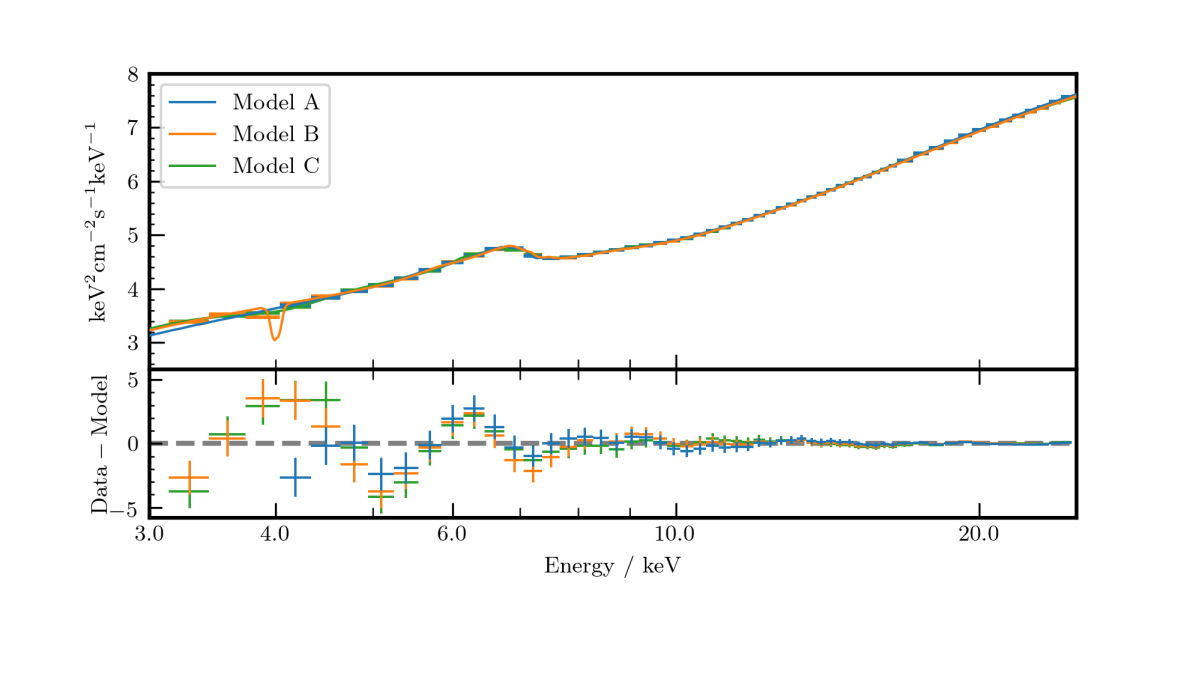
Figure 1: Top Panel: Unfolded time-average spectrum using the reltransDCp (blue and orange) and rtdist (green) reflection models. Bottom panel: residuals of the time averaged spectrum. These models were obtained via fitting the time-averaged and cross spectra simultaneously.

3.1 Model setup

We use the most up-to-date reltrans package (the details of reltrans 2.0 are discussed in Mastroserio et al., 2021). Since our eventual goal is to measure the distance, we use rtdist (Ingram et al., 2022), which is the only model in the package that has distance as a parameter. However, given the version change between M19 and now, we first use reltransDCp to test for consistency with M19 (since this is the closest model in the current package to the models employed by M19). Our strategy is thus to first reproduce the best fit of M19 (or something close) using reltransDCp (Model A), before making several improvements to the M19 analysis (Model B) and finally replacing reltransDCp with rtdist to yield a distance measurement (Model C). Throughout, we include a radial dependence of the ionization parameter $\xi(r)$ and disc electron number density $n_{e}(r)$ by splitting the disc into 20 radial zones (ION_ZONES=20; which we have verified to be adequate to reach convergence). The ionization parameter is defined as

$$\xi(r)=\frac{4\pi F_{x}(r)}{n_{e}(r)},$$ (3)

where $F_{x}(r)$ is the illuminating X-ray ($0.1-1000$ keV) flux, which the model calculates self-consistently. We assume the electron density profile of a zone A Shakura-Sunyaev accretion disc (Shakura & Sunyaev, 1973), an assumption that yielded the best fitting model of M19. We account for the angular dependence of the emergent reflection spectrum (García et al., 2014a) by integrating over 5 angular zones (MU_ZONES=5; which again is adequately converged). Throughout, we fix the BH spin to $a=0.998$ and allow the disc inner radius $r_{\rm in}$ to be a free parameter. This enables us to explore the largest possible range of $r_{\rm in}$ without it becoming smaller than the ISCO. Although these reflection models are sensitive to the BH spin itself, through the null geodesics and energy shifts, they are much more sensitive to $r_{\rm in}$. We freeze the disc outer radius to $r_{\rm out}=2\times 10^{4}\leavevmode\nobreak\ R_{g}$, where $R_{g}=GM/c^{2}$ is the gravitational radius and $M$ is black hole mass. We account for line-of-sight absorption using the xspec model TBabs with the relative abundances of Wilms et al. (2000).

All models we use approximate the corona as a stationary lamppost at height $h$ aligned along the black hole spin-axis; and the accretion disc as Keplerian with a constant aspect ratio $z/r$ where $z$ is the scale height. The aspect ratio in reltransDCp is hard-wired to zero, whereas in rtdist $z/r$ is a model parameter. Preliminary analysis indicated that the rtdist fits were not sensitive to $z/r$, so we fix it to $z/r=0$ for all fits presented here.

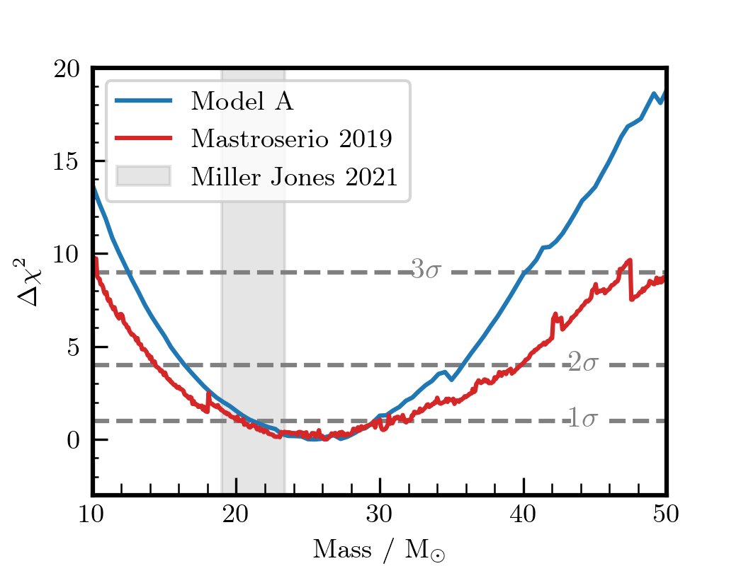
Figure 2: Comparison of the $3\sigma$ mass, $M$, interval obtained in M19 (red) and our Model A (blue). The $3\sigma$ confidence interval obtained in M19 constrains $M\sim 10-50$ M_⊙; while the same confidence interval obtained here constrains $M\sim 15-40$ M_⊙. Both contours agree with the current dynamical mass measurement indicated by the grey shaded region.

3.2 Model A: reproduction of M19

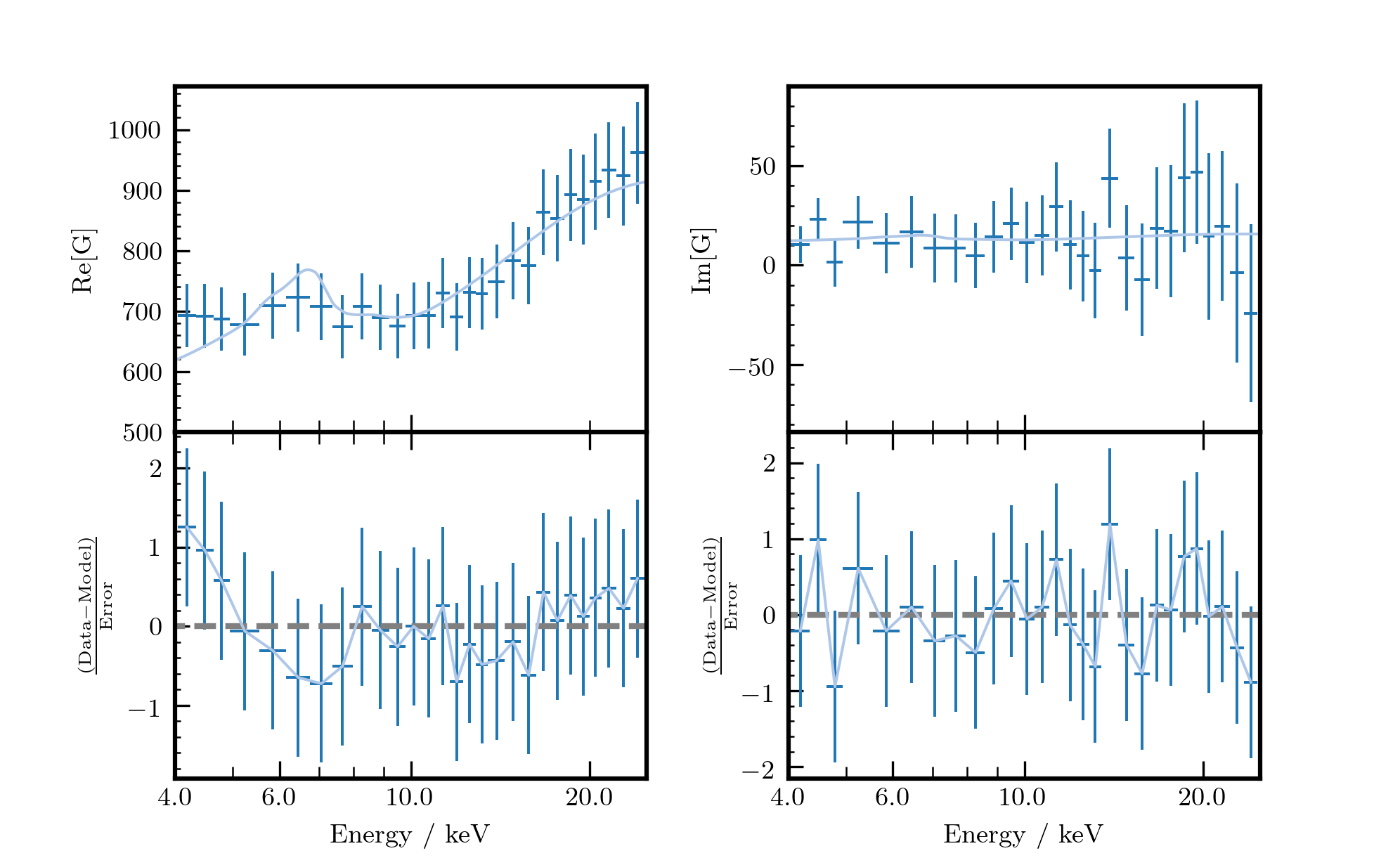
Figure 3: Unfolded cross spectrum (top) and contributions to the overall $\chi^{2}$ (bottom) in a single frequency band ($0.001-0.005$ Hz), with uncertainties calculated using Bendat & Piersol (2000) formulae (Model A). Real and imaginary parts are plotted on the left and right respectively. We see that the error bars are overestimated.

We start by setting up a fit designed to reproduce the M19 results as closely as possible. It is not possible to exactly reproduce the M19 fit due to several bug fixes and extra physics in the latest version of the model. These improvements are described in detail in Mastroserio et al. (2020) and Mastroserio et al. (2021). Another key difference is that the reltrans model used by M19 implements a power law with a high energy cut-off for the continuum, whereas here we use reltransDCp, which implements the thermal Comptonisation model nthcomp (Zdziarski et al., 1996) for the continuum. We are also now fitting to the cross spectrum itself instead of the ‘complex covariance’ (as in M19), but these two statistics differ only in arbitrary normalization.

We use the following model:

$$\texttt{TBabs}\times\texttt{reltransDCp}.$$ (4)

We set the disc density to make the model as similar as possible to the one used in M19. An exact match is not possible, since in old versions of reltrans models, the density was always hardwired to $n_{e}=10^{15}$ cm^-3 for the calculation of the restframe reflection spectrum, whereas in the new models the disc density is a function of radius, $n_{e}(r)$, and the model parameter is the minimum of that function. We fix this minimum density to $n_{e}=10^{15}$ cm^-3. Following M19, we use a reference band of $2.8-3.7$ keV, calculate errors with the BP formula, and only consider the $4-25$ keV energy range in our fits. We refer to this as Model A. Fig. 1 (blue) shows the best-fitting time averaged spectrum, and Table 1 (first column) shows the best fitting parameters. The fit statistic for our Model A is $\chi^{2}/{\rm dof}=492/563$, which is larger than the $\chi^{2}$ for M19 best fitting model (their Model 3).

Fig. 2 shows $\chi^{2}$ versus mass for Model A (blue), alongside that of M19 (red). The low $\chi^{2}$ is due to the use of the BP error formulae to calculate the uncertainties on the real and imaginary parts of the cross spectrum (Ingram, 2019). This can be seen in Fig. 3, which presents the real and imaginary parts of the cross spectrum in one representative frequency range. We see that the error bars are clearly larger than the dispersion of the data around the model, indicating that they are over estimated.

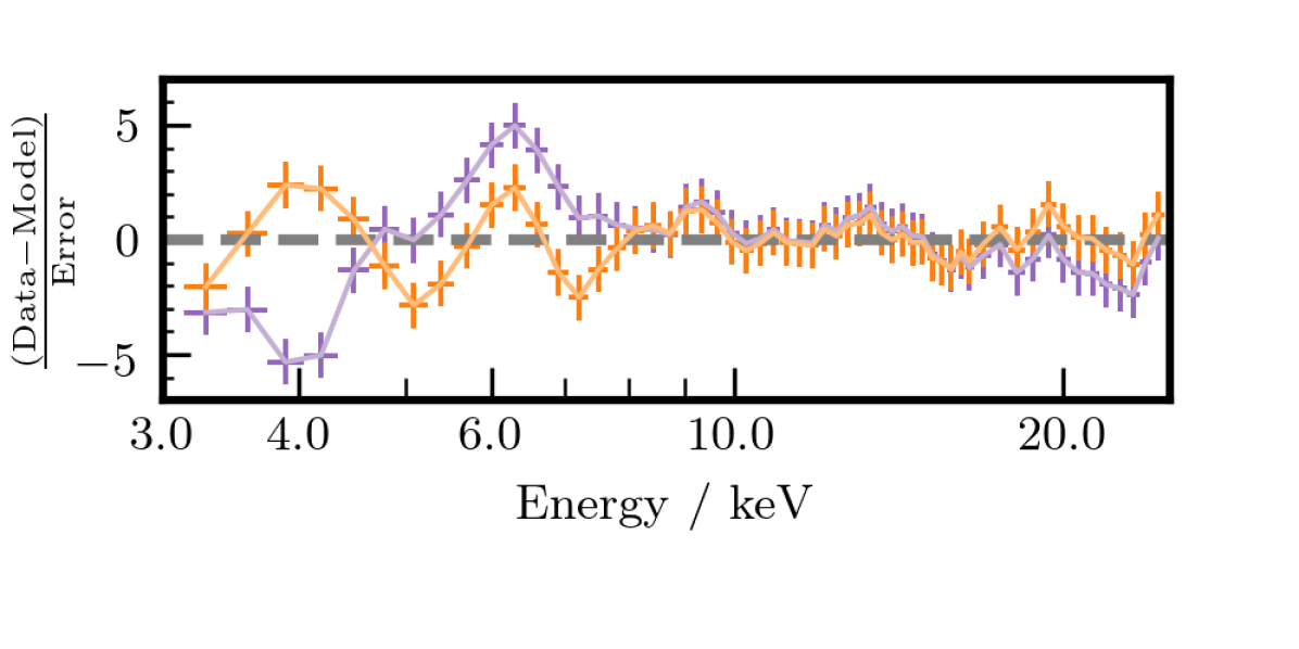
Figure 4: Contributions to $\chi^{2}$ obtained by two models for the time-averaged spectrum (top) and the real part of the cross spectrum in a single frequency band (bottom). Orange points are for our Model B, whereas purple points are for TBabs $\times$ reltransDCp only (i.e. with no disk or calibration components). Although we only show the real part of the cross spectrum for a single frequency band ($\nu\sim 0.001-0.005$ Hz), similarly structured residuals at low energies are present at all frequencies.

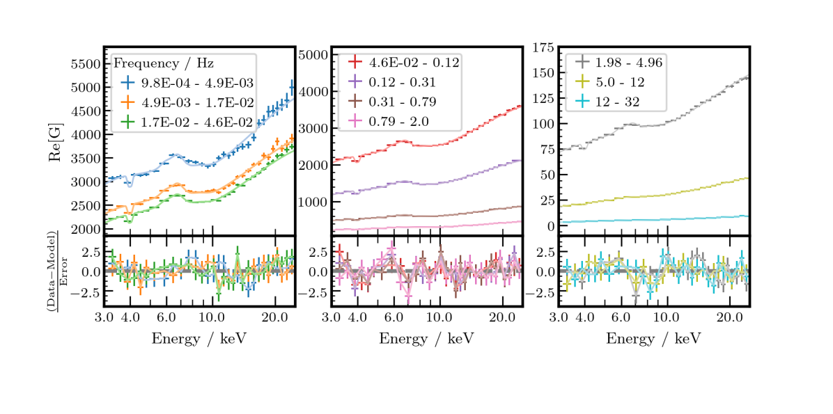
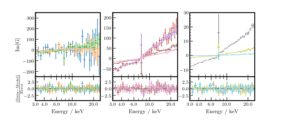
Figure 5: Model B: Unfolded real (top panels) and imaginary (bottom panels) parts of the cross spectrum in all 10 frequency bands. The bottom axis of each panel show the contributions to $\chi^{2}$.

3.3 Model B: free disc density and improved uncertainty estimates

We now improve on M19 whilst continuing to use reltransDCp. In this iteration we make several changes: 1) we allow the minimum disc density $n_{e}$ to be a free parameter. 2) We extend the fitting range to 3-25 keV from 4-25 keV to increase the sensitivity of the model to $n_{e}$. 3) We use the AI error formulae for the cross spectra to address the problem of large error bars, implemented in the original M19 analysis. 4) We increase signal to noise by extending the energy range of the reference band to 3.1-24.7 keV.

Using the above assumptions, we were not able to achieve a good fit (reduced $\chi^{2}$ of $\chi^{2}_{\rm red}\sim 1.6$). This could simply be because the model still does not quite describe the data adequately. The residuals do not look particularly large for any given spectrum, but we fit simultaneously to 21 spectra in total, and so small excesses in $\chi^{2}$ can add up to something larger. We do see some structured residuals in Fig. 1 that become much smaller if we fit only to the time averaged spectrum, indicating that the time average spectrum is in tension with the cross spectra. Alternatively, or additionally, we may now somehow be under estimating the error bars. The choice of reference band does not influence the severity of under fitting, since a broader reference band reduces the true uncertainties in a way that is well represented by the associated reduction in the error bars. We further discuss this under fitting in Section 5.2.

To obtain a reasonable estimate of parameter uncertainties we apply a uniform scaling factor to the cross spectral error bars. The scaling factor was chosen to in order to obtain a $\chi^{2}_{red}\approx 1$ for our Model B fit. We simply increase the cross spectral error bars uniformly by multiplying them by a constant. We hereafter adopt a value of $1.279$ for this multiplicative constant. The cross spectrum error bars in frequency ranges above $5$ Hz are, on average, larger than the BP errors calculated for the respective frequency range by $19-25$ per cent. In frequency ranges below $5$ Hz, our modified errors are smaller than the BP errors; for example in our smallest frequency range ($\sim 0.001-0.005$ Hz) the modified errors are still, on average, $71$ per cent smaller than the BP derived errors. We make no changes at all to the error bars associated with the time-averaged spectrum (beyond the previously mentioned $0.5$ per cent systematic).

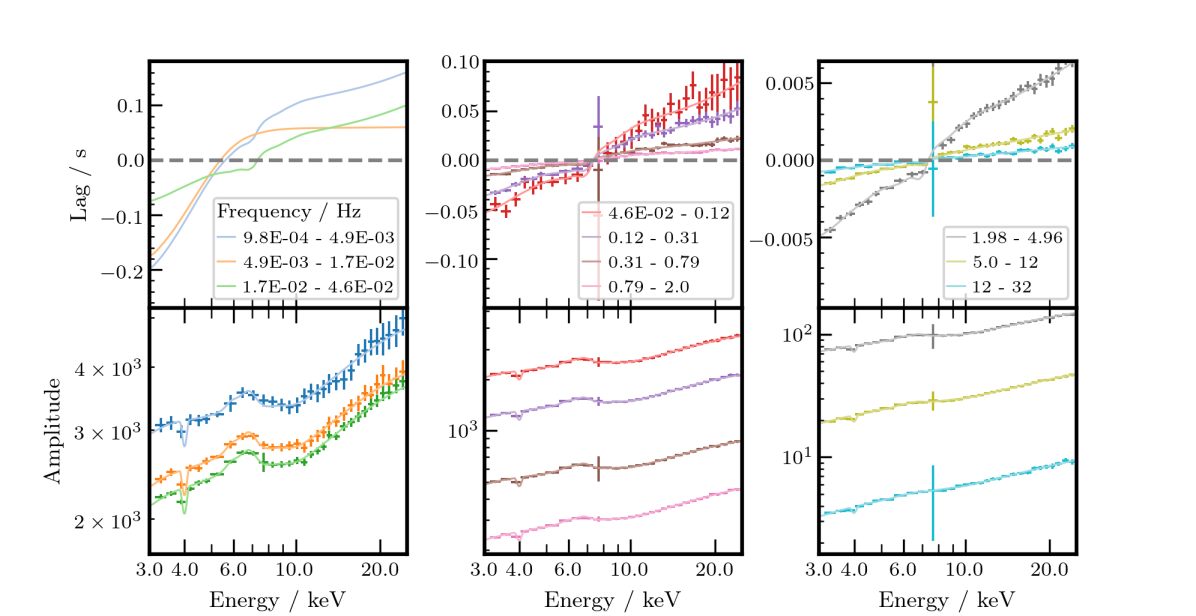
Figure 6: Model B: Lag-energy spectrum (top) and variability amplitude (bottom panels) for different Fourier frequency bands. The points are calculated from the unfolded cross spectra and lines are calculated using parameters of Model B. We only show the model lines for the smallest frequency bands, the data in these frequency bands are not shown due to their large error bars.

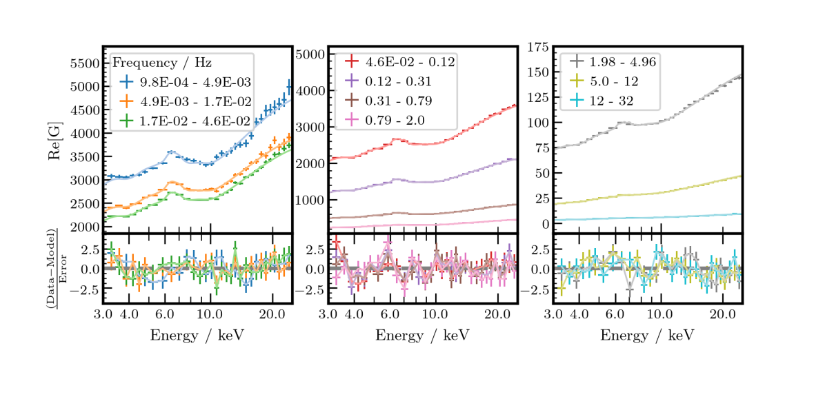
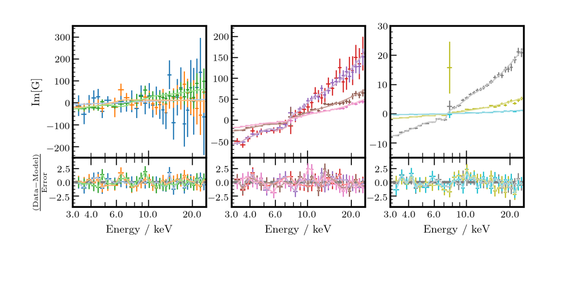
Figure 7: Model C: Unfolded real (top panels) and imaginary (bottom panels) parts of the cross spectrum in all 10 frequency bands. The bottom axis of each panel show the contributions to $\chi^{2}$.

When we performed a fit with the increased cross spectral error bars (i.e. reducing the weight of the cross spectrum during the joint fit), we still see structured residuals at 3-4 keV in the time-averaged and cross spectra: Fig. 4 (purple). We emphasise that the time-averaged spectrum error bars are unchanged. The action of increasing the cross spectral error bars does not intrinsically change the residuals to the time-averaged spectrum, but during a joint fit to the time-averaged and cross spectra, the fitted model is more heavily influenced by the time-averaged spectrum.

We address the low-energy structured residuals by including diskbb in the model for the time-averaged spectrum. This represents thermalised radiation from the disc. The cross spectra exhibit similar residuals, but it is somewhat unphysical to add a diskbb component to the cross spectrum, which would represent rapid variability of the emission from the entire disc. It is much more likely that disc variability is dominated by radiation from the inner disc. We therefore add a blackbody component (bbody) to the cross spectral model. All cross spectrum blackbody temperatures were tied to one another, but were not tied to the time-average diskbb temperature. This means that the blackbody component represents variable blackbody emission from a single radius of the accretion disc. The bbody temperature being equal to the diskbb temperature corresponds to variability originating from $r_{\rm in}$, whereas the bbody temperature being less than the diskbb temperature corresponds to the variable radius being larger than $r_{\rm in}$. In reality, this approximates the variability coming from a narrow range of disc radii.

The bbody normalization, $N_{\rm{BB}}$, is an independent free parameter for the real and imaginary parts of the cross spectrum of each frequency range. The normalization evolving with frequency is indicative of the power spectrum of disc variability. The normalization of the imaginary part of the cross spectrum in a given frequency range relates to the time lag between the disc variability and the reference band variability at that frequency. Specifically, the normalization of the imaginary part being larger than zero would indicate the disc variability lagging the variability in the reference band.

We also find evidence of a $\sim 4$ keV calibration feature, similar to that previously reported by García et al. (2014b) for the Crab and Connors et al. (2020) for XTE J1550-564. García et al. (2014b) developed the tool pcacorr to correct for such features, but unfortunately our data were taken too early in the RXTE mission for pcacorr to be applicable. We instead include a Gaussian absorption line with gabs. This feature could additionally be accounting for variable line-of-sight absorption, which is known to be present in the Cyg X-1 spectrum (Lai et al., 2022).

The model we use is:

$$\texttt{TBabs}\times\texttt{gabs}\times(\texttt{diskbb}+\texttt{bbody}+\texttt{reltransDCp}).$$ (5)

This is the model we fit to both the time averaged and cross spectrum simultaneously. The model is initialised such that the parts that affect the time-averaged spectrum are given by:

$$\texttt{TBabs}\times\texttt{gabs}\times(\texttt{diskbb}+\texttt{reltransDCp}),$$ (6)

and the cross spectrum is affected by:

$$\texttt{TBabs}\times\texttt{gabs}\times(\texttt{bbody}+\texttt{reltransDCp}).$$ (7)

The model parameters of TBabs and gabs are tied between the time averaged spectrum and all cross spectra. The diskbb normalization is a free parameter for the time averaged spectrum, and is frozen to zero for all cross spectra. Conversely, the bbody normalization is frozen to zero for the time-averaged spectrum and is free for the cross spectra. Within reltransDCp model, certain parameters are also tied between the time-averaged data and the cross spectra (such as lamppost height). However there are Fourier frequency dependent spectral pivoting parameters, $\phi_{\rm{AB}}$ and $\gamma$, that are used to model the cross spectrum in specific frequency bands. These parameters relate to the phase difference and amplitude ratio of spectral index and normalization variability respectively. For the time-averaged spectrum $\phi_{\rm{AB}}=\gamma=0$; for the cross spectrum $\phi_{\rm{AB}}$ and $\gamma$ are free parameters that are tied between real and imaginary parts of the cross spectrum in a given frequency band. For example, we need 10 $\phi_{\rm{AB}}$ and $\gamma$ to model the real and imaginary parts of the cross spectrum (i.e. one set of $\phi_{\rm{AB}}$ and $\gamma$ are used to calculate the cross spectrum in a defined frequency range). We further discuss $\phi_{\rm{AB}}$ and $\gamma$ in Appendix B.

We obtain a good fit with $\chi^{2}/{\rm dof}=586/599$; which we refer to as Model B. We list the best fitting parameters in Table 1, and show our fit to the time averaged spectrum in Fig. 1 (orange points). Fig. 5 shows the fits to all cross spectra. We show real (top) and imaginary (bottom) parts of the cross spectrum in each of the 10 frequency bands (as labelled). The data are unfolded around the best fitting model. In Fig. 6, we convert the real and imaginary parts of the cross spectra into time lag (top) and absolute variability amplitude (bottom). The data were converted from the unfolded real and imaginary parts of the cross spectra. We do not plot the lag data for the lowest frequency ranges due to the error bars being very large. Although the real and imaginary parts of the cross spectrum were used in the fit (for statistical reasons detailed in Mastroserio et al. 2018), the lag and amplitude are easier to interpret physically. We see a dip at the iron line of the model lag spectra, which is due to the reverberation lag being smaller than the continuum lag (Mastroserio et al., 2018). We also see the reflection features in the amplitude spectrum becoming less prominent with increasing frequency, which is due to the finite size of the reflector washing out fast variability in the reflected signal via path length differences (Revnivtsev et al., 1999; Gilfanov et al., 2000).

3.4 Model C: distance measurement

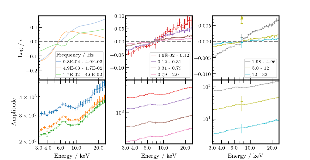
Figure 8: Model C: Lag-energy spectrum (top) and variability amplitude (bottom panels) for different Fourier frequency bands. The points are calculated from the unfolded cross spectra and lines are calculated using parameters of model C. We only show the model lines for the smallest frequency bands, the data in these frequency bands are not shown due to their large error bars.

We now replace reltransDCp used in model B with rtdist. The headline difference between these two models is that rtdist takes distance $D$ as an input in place of the peak ionization parameter $\log\xi$, which is instead self-consistently calculated (Ingram et al., 2022). There are some other more subtle differences between reltransDCp and rtdist. Most importantly, the boost parameter is treated differently. In reltransDCp, the relative normalization of the direct and reflected components is set to the value calculated self-consistently for a stationary, isotropically emitting lamppost corona multiplied by boost (Ingram et al., 2019). In this way, the amount of reflection in the spectrum is artificially increased from the calculated value if $\texttt{boost}>1$. This is designed to account for the isotropic lamppost assumption surely being an over simplification. In rtdist   the boost parameter instead adjusts the angular emissivity of the lamppost corona. Setting boost$>1$ now beams radiation towards the black hole, which increases the amount of reflection in the output spectrum and leads to reflection being more centrally concentrated on the disc (i.e. the radial emissivity profile becomes steeper). This is in principle a more self-consistent treatment than that employed in the earlier reltrans models. The rtdist model also includes the parameters $b_{1}$ and $b_{2}$, which further distort the angular emissivity profile of the corona away from isotropic if they are non-zero. For $\texttt{boost}=1$ and $b_{1}=b_{2}=z/r=0$, the two models are able to output identical results, as long as the user finds the value of $D$ in rtdist that corresponds to the peak ionisation parameter used for reltransDCp. The two models otherwise diverge. We find that our fits are insensitive to $b_{1}$ and $b_{2}$ and so freeze them to zero (as well as $z/r$). We see from Table 1, however, that the best fitting Model B boost parameter is $\texttt{boost}\approx 0.29$, and so we already know that we will not be able to exactly reproduce the Model B fit with rtdist in place of reltransDCp.

We use the same procedure described in the previous subsection to implement the model

$$\texttt{TBabs}\times\texttt{gabs}\times(\texttt{diskbb}+\texttt{bbody}+\texttt{rtdist}),$$ (8)

and we refer to our best fit using this as Model C. As was the case with Model B, the calculated time-averaged spectrum and cross spectra are affected by parameter changes in the components outlined in equations 6 & 7 respectively, albeit reltransDCp is now replaced with rtdist. Our best fit is $\chi^{2}=654/599$; we show our fit to the time average spectrum in Fig. 1 (green); the cross spectra in Fig. 7; and list our best-fitting parameters in Table 1. In Fig. 8, we again convert the real and imaginary parts of the cross spectra to time lag and variability amplitude. We again see the dip at the iron line of the lag models and the weakening of reflection features with increasing frequency in the amplitude spectrum.

Model	Model A	Model B	Model C
Absorption Model	TBabs	TBabs	TBabs
$N_{H}$ / $10^{22}$	$1.30^{+0.08}_{-0.13}$	$1.61263^{+0.3}_{-0.2}$	$2.1^{+0.2}_{-0.1}$
Absorption Line Model		gabs	gabs
E / keV	—	$4.00^{+0.03}_{-0.03}$	$4.00^{+0.05}_{-0.05}$
Width / keV	—	$0.03^{+0.06}_{-0.02}$	$0.46^{+0.10}_{-0.06}$
Strength	—	$0.022^{+0.003}_{-0.004}$	$0.07^{+0.02}_{-0.01}$
Time-average Blackbody Model		diskbb	diskbb
$kT_{in}$ / keV	—	$0.80^{+0.03}_{-0.04}$	$1.09^{+0.03}_{-0.03}$
normalization	—	$155^{+58}_{-36}$	$72^{+16}_{-7}$
Cross spectrum Blackbody Model		bbody	bbody
$kT$ / keV	—	$0.640^{+0.02}_{-0.004}$	$0.76^{+0.04}_{-0.04}$
Reflection Model	reltransDCp	reltransDCp	rtdist
$h$ / $R_{g}$	$10.5^{+0.5}_{-0.8}$	$11.2^{+0.3}_{-0.5}$	$9.59^{+0.05}_{-0.1}$
$i$ / ∘	$37.5^{+1.1}_{-0.9}$	$37.9^{+1.1}_{-0.9}$	$43.8^{+2.0}_{-1.1}$
rin / $R_{g}$	$4.7^{+0.7}_{-0.9}$	$5.7^{+0.2}_{-0.2}$	$24.90^{+0.04}_{-0.04}$
$\Gamma$	$1.737^{+0.007}_{-0.004}$	$1.700^{+0.006}_{-0.006}$	$1.702^{+0.002}_{-0.004}$
D / kpc	—	—	$2.7^{+0.2}_{-0.6}$
log $\xi$	$3.40^{+0.03}_{-0.01}$	$3.36^{+0.02}_{-0.04}$	—
$A_{Fe}$	$1.8^{+0.2}_{-0.1}$	$2.5^{+0.2}_{-0.1}$	$0.89^{+0.04}_{-0.03}$
log $n_{e}$	$15.0$	$18.5^{+0.3}_{-0.3}$	$19.56^{+0.10}_{-0.07}$
$kT_{e}$ / keV	$138^{+92}_{-45}$	$178^{+32}_{-24}$	$378^{+20}_{-36}$
boost	$0.37^{+0.01}_{-0.01}$	$0.29^{+0.01}_{-0.01}$	$0.32^{+0.05}_{-0.1}$
$M$ / M⊙	$25.1^{+6.7}_{-6.6}$	$16.5^{+4.8}_{-3.9}$	$13.9^{+1.4}_{-3.3}$
normalization	$0.092^{+0.007}_{-0.004}$	$0.097^{+0.003}_{-0.001}$	$0.1060^{+0.002}_{-0.0008}$
$\chi^{2}$	$492/563$	$586/599$	$654/599$

Table 1: Best fitting parameters obtained from $\chi^{2}$ minimization from to the cross spectrum in 10 frequency ranges ($0.98$ mHz - $32$ Hz) and the time-average spectrum. In both models the spin was fixed to 0.998. In reltransDCp distance is not a parameter hence is not included. In rtdist, log$\xi$ is internally calculated hence is not a free parameter. Errors are all $90$ per cent confidence. We do not list the empirical parameters for each frequency band, i.e. the bbody normalizations ($N_{\rm BB}$) for real and imaginary parts, and the reltrans continuum lag parameters $\phi_{\rm{AB}}$ and $\gamma$. We instead summarise the empirical parameters in Appendix B.

4 Results

Table 1 lists the best-fitting parameter values of all three models alongside the corresponding fit statistic. For Model A we obtain parameter uncertainties using the xspec error command, whereas for Models B and C we estimate errors from Monte Carlo Markov Chain (MCMC) simulations. We initialise the MCMC simulation from the best fitting models B and C found via $\chi^{2}$ minimization. For model B and C we run one chain each, where the total number of steps in both chains were 307456 with an initial burn-in of 19968. We use 256 walkers in both chains. For each parameter in both chains we find the Geweke convergence measure to be within the range -0.2 to 0.2, indicating convergence.

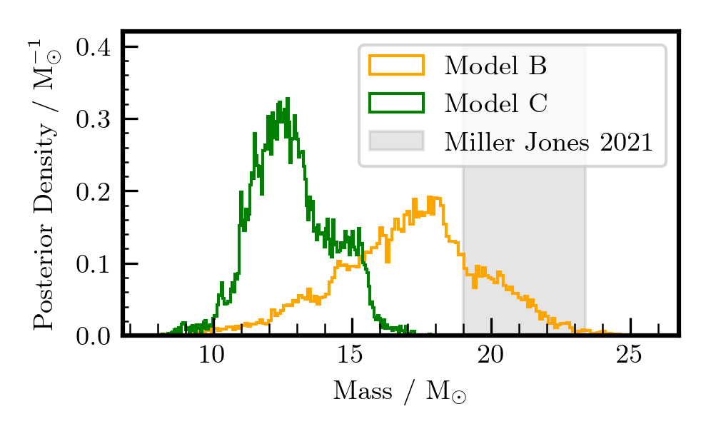
Figure 9: Histograms showing the MCMC posterior densities (as a fractional quantity) for the black hole mass $M$, using our models B and C.

4.1 Mass and distance

Black hole mass is a parameter in all three of the models summarised in Table 1. However, Model A is only intended as a consistency check with M19, and thus we do not discuss it further. Fig. 9 shows the mass posteriors obtained from Models B and C, alongside the dynamical measurement of Miller-Jones et al. (2021). We see that the Model B value is consistent with the dynamical measurement, whereas the Model C value is lower. The only material difference between the two models is how the boost parameter is treated, which we will discuss in Section 5. The peak posterior values of the mass differ slightly from the minimum $\chi^{2}$ values presented in Table 1, but well within $1\leavevmode\nobreak\ \sigma$ uncertainties.

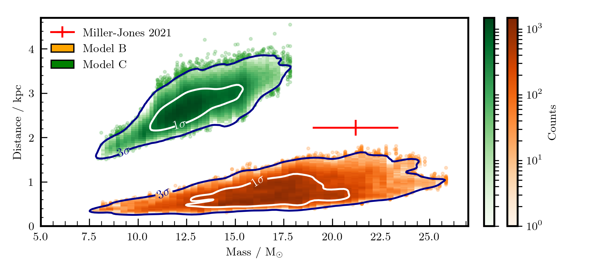
Figure 10: Distance and mass contour for the Model B and C fits (as labelled). We also show the accepted distance measurement and inferred black hole mass for Cyg X-1. The white and blue lines are the $1\sigma$ and $3\sigma$ contours; inside the contours the color scale indicates the number of walkers within the bin.

Model C, which uses rtdist, is the only model that takes distance as an input parameter. We note, however, that distance can also be inferred from Model B, which instead uses reltransDCp. We use a post-processing code to convert the peak ionization parameter of reltransDCp to distance. The code uses Equation (10) of Ingram et al. (2022), which relates the ionization parameter $\xi(r)$ to the distance via the radial emissivity profile, $\epsilon(r)$. For rtdist, $\epsilon(r)$ is defined by Equation (6) of Ingram et al. (2022). In our post processing code, we instead use the definition of $\epsilon(r)$ from Equation (20) of Ingram et al. (2019), multiplied by boost. This the emissivity profile that is employed in reltransDCp, which assumes a stationary, isotropic lamppost before artificially adjusting the reflected flux by a factor boost. The post processing code, which will be available in future public releases of the reltrans package, reads in an MCMC table output from reltransDCp fits and adds a column consisting of a distance value for each step in the chain.

For both Models B and C, we apply further post processing to the distance values to account for absolute flux uncertainty (following Nathan et al., 2024). For each step in the chain, we estimate the true distance $D$ as

$$D=\frac{D_{0}}{\sqrt{x(1+\eta)}},$$ (9)

where $D_{0}$ is the ‘raw’ distance measurement output by the model, $x$ is a constant that accounts for the known systematic flux offset of the instrument, and $\eta$ is a Gaussian random variable with zero mean and a standard deviation of $\sigma$ that accounts for calibration uncertainty. We use $x=9.5/10.7$, since García et al. (2014b) measure the normalization of the power-law spectrum of the Crab nebula to be $\approx 10.7$ for the earliest epochs of the RXTE mission (which are most relevant to our dataset), whereas the accepted value is $\approx 9.5$ (Toor & Seward, 1974). We set $\sigma=0.1$ to conservatively employ a $10$ per cent absolute flux uncertainty for RXTE, following e.g. Steiner et al. (2012). Note that flux $\propto 1/D^{2}$, thus the inferred distance goes as one over the square root of flux. This means that a $10$ per cent flux uncertainty translates to a $5$ per cent distance uncertainty.

Fig. 10 shows the resulting joint mass-distance posterior for Models B and C. We see that both models return reasonable values for mass and distance, but both formally disagree with the dynamical/parallax values (red cross).

4.2 Disc variability

Models B and C include a diskbb component in the time averaged spectrum and a bbody component in the cross spectra. For the best fit of both models, the bbody temperature is slightly lower than the peak diskbb temperature. This corresponds physically to a disc that is accreting stably through most of its extent but exhibits variability at some narrow range of radii in its inner regions, as suggested by e.g. Wilkinson & Uttley (2009); Rapisarda et al. (2016). Since the disc temperature goes as $T/T_{\rm in}=(r/r_{\rm in})^{-3/4}$ in the diskbb model, we can estimate that the outer radius of the variable region in the disc is $(T_{\rm in}/T)^{4/3}\leavevmode\nobreak\ r_{\rm in}\sim 1.5\leavevmode\nobreak\ r_{\rm in}$ for both models.

In Fig. 11, we show how the best fitting bbody normalization parameters depend on Fourier frequency. The parameters we fit for are the normalizations of the real and imaginary components, $N_{\rm{BB},\rm{real}}$ and $N_{\rm{BB},\rm{im}}$. However, it is more instructive to plot in terms of amplitude and phase. The bottom panel shows variability amplitude, $\sqrt{N_{\rm{BB},\rm{real}}^{2}+N_{\rm{BB},\rm{im}}^{2}}$. We see that this decreases with Fourier frequency, which is expected since high frequency variability is expected to be damped by viscous processes (e.g. Lyubarskii, 1997; Frank et al., 2002). The top panel shows time lag, $\arctan(N_{\rm{BB},\rm{im}}/N_{\rm{BB},\rm{real}})/(2\pi\nu)$. Due to the sign convention, this shows that disc variability leads variability in the reference band. This is again expected physically for disc variability driven by accretion rate fluctuations, since those fluctuations will propagate inwards on a viscous timescale before modulating the coronal flux (Lyubarskii, 1997; Uttley & Malzac, 2025).

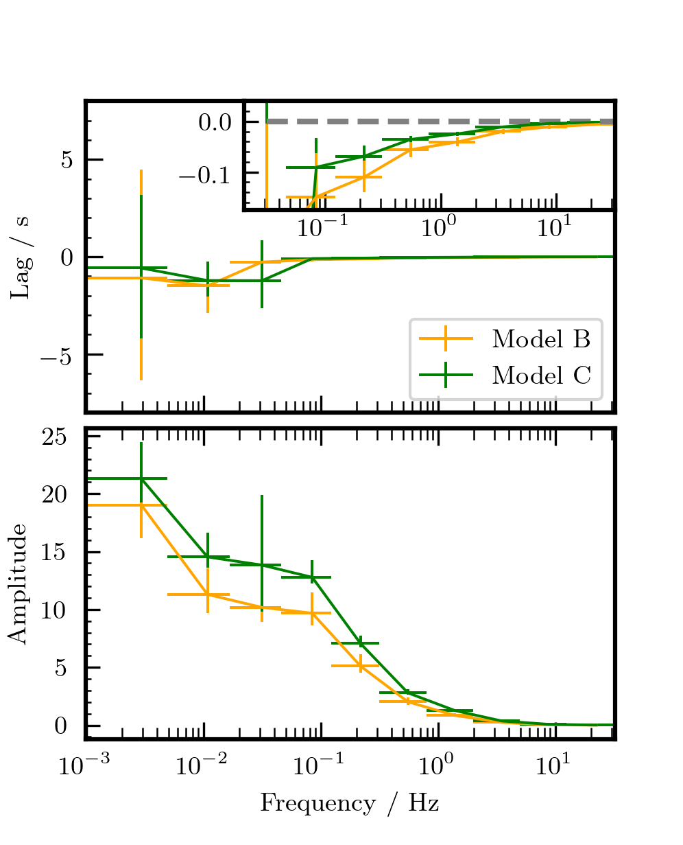
Figure 11: Lag-frequency spectrum (top) and variability amplitude (bottom) associated with the bbody obtained from the models B & C with our best fit parameters. The inset axis in the top panel is the zoomed-in region of the higher frequency lags. We measure negative lags, indicating that variability in the blackbody component leads that in the reference band. Error bars shown are the 90 per cent confidence interval.

Fig. 12 demonstrates the influence of disc variability on the overall time lags in the model. Since disc variability is only prominent at low frequencies, we only plot for three low frequency ranges. The dashed lines show the lags resulting from spectral pivoting alone; i.e. the reflection and disc components have both been switched off. We see only the log-linear lags that result from spectral pivoting (Kotov et al., 2001; Mastroserio et al., 2018). The solid line is still without reflection, but now includes disc variability as well as spectral pivoting. We see that the disc contributes a negative lag at soft X-rays, due to disc variability leading coronal variability. Note that here we plot only for Model B, since for reltransDCp it is easy to switch off the reflection component, but very similar properties are also seen for Model C. Details of the reltrans spectral pivoting parameters $\phi_{AB}$, $\gamma$; and bbody parameters $N_{\rm{BB},\rm{real}}$, $N_{\rm{BB},\rm{im}}$ is given in Appendix B.

4.3 Other parameters

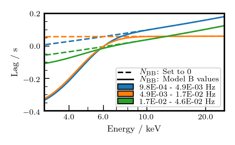
Figure 12: Collection of the model predicted lag-energy spectra for Model B in the lowest frequency bands, with reflection switched off (boost=0). Since reflection is switched off, there are no reverberation lags. The dashed lines are when disc variability is also switched off, leaving only the log-linear continuum lags. The solid lines include disc variability, which we see contributes a negative lag at lower energies.

We see from Table 1 that several parameters are consistent across all three models, including the source height $h\sim 10\leavevmode\nobreak\ R_{g}$ and the boost parameter boost $\sim 0.3$. The latter indicates that the reflection fraction is smaller than that expected from a stationary, isotropic lamppost model. The inclination varies moderately across the three models from $i\approx 38^{\circ}$ to $i\approx 44^{\circ}$, all of which are larger than the binary inclination (Miller-Jones et al., 2021).

One striking difference between Models B and C is the disc inner radius, which is $r_{\rm in}\approx 6\leavevmode\nobreak\ R_{g}$ for Model B and $r_{\rm in}\approx 25\leavevmode\nobreak\ R_{g}$ for Model C. This emphasises that the measured inner radius can be very dependent on model assumptions, as has been discussed many times previously (e.g. Shreeram & Ingram, 2020; Basak et al., 2017; Zdziarski et al., 2021, 2022). We note, however, that Model B has a much lower $\chi^{2}$ than Model C. Another key difference is the (minimum) electron density. This is fixed to $n_{e}=10^{15}\leavevmode\nobreak\ {\rm cm}^{-3}$ in Model A, and rises to $n_{e}\approx 10^{18.5}\leavevmode\nobreak\ {\rm cm}^{-3}$ for Model B and $n_{e}\approx 10^{19.6}\leavevmode\nobreak\ {\rm cm}^{-3}$ for Model C. This difference in density correlates strongly with the different distance and mass returned by the two models. If all other parameters are kept the same, $n_{e}\propto(D/M)^{2}$. The ratio of densities (Model C / Model B) is $\sim 13$ and the ratio of $(D/M)^{2}$ is $\sim 22$, so to within a factor of $\sim 2$, the different $D/M$ ratio derived from the two models is simply driven by the different density measurement.

The density also likely trades off with the iron abundance $A_{\rm Fe}$, which is super-solar for Model B and roughly solar for Model C. This is consistent with the conclusion of Tomsick et al. (2018). Finally, the electron temperature $kT_{e}$ is a lot higher for Model C compared with the other two models. Our data only extend to $25$ keV, so we are not directly sensitive to $kT_{e}$, but we are indirectly sensitive through its influence on the shape of the restframe reflection spectrum (García et al., 2015). The different electron temperatures exhibited by Models B and C therefore indicates that these two models feature slightly different restframe reflection spectra, which perhaps partly explains the different derived inner radii. A direct constraint on $kT_{e}$ with hard X-ray coverage (e.g. Krawczynski et al., 2022) would therefore break an important degeneracy in spectral shape.

5 Discussion

We have conducted an X-ray reverberation mapping analysis on RXTE data of Cyg X-1 in the hard state using models from the reltrans package. This has enabled us to make the first estimate of distance to a BHXB through X-ray reverberation mapping.

5.1 Disc variability

This work builds upon earlier work on the same dataset by M19. One motivation to revisit the dataset was to address the problem presented by unphysically large error bars that were implemented during the M19 analysis. Using the error formulae for the cross spectra from Ingram (2019), coupled with the extension of the low band pass considered for our fit from 4 to 3 keV, reveal the need for disc variability. Our results are consistent with the disc accreting stably outside of $r\sim 1.5\leavevmode\nobreak\ r_{\rm in}$, with accretion rate variability becoming prominent inside of that radius. We find that the disc variability leads variations in the reference band, which is dominated by the corona. This is consistent with mass accretion rate variations propagating inwards from the disc before eventually reaching the corona after a propagation time (Wilkinson & Uttley, 2009; Rapisarda et al., 2016). Fig. 11 (top) shows that the observed lag is $\sim 1$ s at the lowest frequencies, and gets shorter with increasing frequency. This reduction of the lag with increasing frequency occurs in the propagating fluctuations model because the characteristic variability frequency generated in the disc – the viscous frequency – increases with decreasing radius (e.g. Lyubarskii, 1997; Churazov et al., 2001; Frank et al., 2002; Mushtukov et al., 2018). Since the highest frequency variability can only be generated in the inner disc, it cannot have propagated far. On the other hand, low frequency variability can be generated further out in the disc and thus the observed low frequency lags include contributions from variability that has propagated a long distance (Arévalo & Uttley, 2006; Ingram & van der Klis, 2013). Thus, if the observed disc variability is indeed driven by accretion rate fluctuations, the true propagation lag from the edge of the variable region ($r\sim 1.5r_{\rm in}$ in this case) to the corona is longer than the observed lag of $\sim 1$ s. Fig. 11 (bottom) shows that the amplitude of disc variability is roughly constant at lower frequencies (except for the lowest frequency band, which shows an excess), and starts to drop off above $\nu\sim 0.1$ Hz. This drop off is again expected in the propagation fluctuations model, and can be interpreted as a lower limit for the local viscous frequency in the variable region of the disc. The viscous frequency at $r_{\rm in}$ sets the fastest characteristic variability timescale in the disc mass accretion rate. The observed radiation is the sum of that emitted from different regions of the disc, and interference between signals from different regions washes out variability at the highest frequencies, leaving the observed break at a frequency lower than the peak viscous frequency (Ingram & van der Klis, 2013). In future it may be possible to quantitatively apply a detailed propagating fluctuations model to the disc variability observed here (following e.g. Rapisarda et al., 2017).

Disc variability has also been suggested to drive the fluctuations in the power law index of the corona that the reltrans models input in an ad hoc manner to reproduce the continuum lags. Uttley & Malzac (2025) showed that an over-density in the disc first leads to cooling of the corona via an increase in seed photons, then after a propagation time heats the corona (also see Karpouzas et al. 2020). The instantaneous power law index can be approximated as $\Gamma(t)\approx\Gamma_{0}[L_{s}(t)/L_{h}(t)]^{1/6}$ (Beloborodov, 2001), where $\Gamma_{0}$ is the time-averaged photon index, $L_{s}(t)\propto\dot{M}(1.5r_{\rm in},t)$ is the seed photon luminosity and $L_{h}(t)\propto\dot{M}(1.5r_{\rm in},t-\Delta t)$ is the coronal heating luminosity. Whereas here we simply parameterise $\Gamma(t)$ fluctuations and their delay with respect to luminosity variations with the parameters $\gamma$ and $\phi_{AB}$ (see Fig. 13), in future we may be able to self-consistently calculate $\Gamma(t)$ variations from disc variability in the framework of the Uttley & Malzac (2025) model.

5.2 Fit quality

Even after including disc variability in our model, we still obtain a rather high $\chi^{2}$ while using AI cross spectrum error formulae with our implemented scaling factor (see sec 3.3). There is some structure to the residuals presented in Figs 5 and 7, specifically at photon energies $<4$ keV for low-mid frequencies and $\sim 6$ keV for mid frequencies. A comparison of the structured residuals present in Figs 5 and 7 show that the location and shape of the structure are similar across the different model implementations. The presence of structured residuals in only a few frequency ranges at specific energies could be an indication that the lamppost models are too simplistic to capture the microphysics made apparent by smaller cross spectrum uncertainties. Alternatively the structured residuals could indicates that cross spectrum errors (using the AI error formulae and our scaling factor) are somehow being underestimated. The problem could be that intrinsic source variability causes the real and imaginary parts of the cross spectrum to be correlated with one another, whereas here we treat them as independent quantities during fitting. If there is correlation, then the procedure we follow here is not formally appropriate. We will investigate cross spectral statistics in detail in a future publication (Nathan et al in prep). For the purposes of this paper, we simply increased the cross spectral uncertainties by a constant factor to get a reasonable estimate of parameter uncertainties.

5.3 Geometrical parameters

We fit three models, referred to as Models A, B and C (see Table 1). Model A is purely intended to verify consistency with the earlier work of M19, which it does successfully. Models B and C are the fits worth further discussion. These two models differ only in their treatment of the reflection fraction, which is controlled in both cases by the boost parameter. This parameter is found to be boost $\approx 0.3$ for both fits, but the meaning of this parameter is quite different for the two models. Model B uses reltransDCp (Mastroserio et al., 2021), which calculates the reflection fraction self-consistently for a stationary, isotropic lamppost source before artificially adjusting the normalization of the reflection spectrum by a factor boost. This adjustment is intended to account for the over-simplified nature of the lamppost model. For Model C, which uses rtdist (Ingram et al., 2022), the boost parameter adjusts the angular emissivity of the corona (i.e. boosts emission towards or away from the black hole). Thus boost $<1$ reduces the reflection fraction from the simple isotropic case for both models, but for Model B the shape of the reflection spectrum is unchanged, whereas for Model C the iron line is slightly narrower due to the coronal emission being boosted away from the black hole, thus resulting in less centrally peaked illumination of the disc.

These two models yield quite different measurements of disc inner radius: $r_{\rm in}\approx 6\leavevmode\nobreak\ R_{g}$ for Model B and $r_{\rm in}\approx 25\leavevmode\nobreak\ R_{g}$ for Model C. In the truncated disc model, $r_{\rm in}$ is expected to be reasonably large in the hard state (consistent with our Model C); backed up by Hard X-ray Modulation Telescope observations of Cyg X-1 (Feng et al., 2022); where they find the truncation radius decreases as the source softens. On the contrary, several reflection modelling studies find that the disc already reaches the ISCO in the bright hard state (García et al., 2015; Liu et al., 2023). Model C is certainly consistent with the truncated disc picture, although we note that Model B has a significantly lower $\chi^{2}$. The Model B value, although smaller, is still outside of the ISCO for a rapidly spinning black hole, which Cyg X-1 has been suggested to be (Zhao et al. 2021, but see Belczynski et al. 2021 for a contrasting view). However, our results here cannot contribute to the debate of whether the disc reaches the ISCO in the bright hard state, since Cyg X-1 is thought to always be on the lower branch of the HID (luminosity $\sim 2$ per cent Eddington). The sensitivity of the inferred disc inner radius to assumptions that we experience in our fits is representative of many other studies in the literature (e.g. compare Buisson et al. 2019 with Zdziarski et al. 2021; or Parker et al. 2015 with Basak et al. 2017).

Our fits yield an inclination angle slightly higher than the known binary system inclination: $i\approx 38^{\circ}$ and $i\approx 44^{\circ}$ for Models B and C compared with a binary inclination of $i\approx 27.5^{\circ}$ (Miller-Jones et al., 2021). This is consistent with results of previous time-averaged spectral studies, both in the soft state ($i>38^{\circ}$: Tomsick et al. 2014; Walton et al. 2016) and in the hard state ($i>42^{\circ}$: Parker et al. 2015). Although the inclination angle inferred from reflection modelling is subject to systematic uncertainty, it is interesting to consider the case for Cyg X-1 having a warped disc, such that we see the inner disc and corona from a higher inclination than the outer disc, which presumably aligns in the binary plane. Indeed, such a misalignment is required for simple Comptonising slab corona models to explain the unexpectedly high 2–8 keV polarization degree of $4$ per cent measured by IXPE (Krawczynski et al., 2022). An alternative explanation that allows for an aligned system invokes a $\sim 0.4c$ bulk outflow velocity of the electrons in the corona (Poutanen et al., 2023). In principle it is possible to obtain an outflow velocity from the boost parameter for Model C, however it is not so straightforward. What we can say is that, boost $<1$ is consistent with an outflow, but we can’t be more quantitative because the influence of an outflow on the emissivity profile will be sensitive to the unknown true coronal geometry. In any case, the polarization aligns with the jet (Krawczynski et al., 2022), which indicates that the corona is extended in the disc plane. This is formally incompatible with the lamppost model we employ here, although we stress that our use of the lamppost model is purely out of mathematical and computational convenience. There are two lines of thought concerning a radially extended (pancake) corona. Hypothetically, if the pancake corona is suspended a distance $h$ above the BH (as is the case for the lamppost), it may predict light crossing delays comparable to those predicted by the lamppost model if the radial extension of the corona is small compared with $h$. If the pancake corona instead exists in the equatorial disk plane, the light crossing delays will be drastically different to those predicted by the lamppost model, and will depend on the radial extent of the corona.

5.4 Mass and distance

Both Models B and C yield estimates of distance and black hole mass (Fig. 10). For Model C, distance is a model parameter, whereas for Model B we infer the distance from other parameters using a post processing code that will be made available in a future public release of the reltrans package. It is very encouraging as a proof of principle that both models yield reasonable ball-park figures of these parameters: $M\sim 18\leavevmode\nobreak\ M_{\odot}$, $D\sim 1$ kpc for Model B, and $M\sim 12\leavevmode\nobreak\ M_{\odot}$, $D\sim 2.5$ kpc for Model C. Note that we employ no priors, and there is nothing in the models that requires the mass and distance to be in the expected range. Both could have been orders of magnitude out, but are not. There are many approximations in the models that could have dramatically affected accuracy. For example, the illuminating spectrum is calculated with nthcomp (Zdziarski et al., 1996), with the seed photon temperature that determines the low energy cut off hardwired to $0.01$ keV. This value is unrealistically low (if the seed photons for Comptonisation are provided mainly by the disc), and so the disc ionization state is calculated within the model assuming the wrong illuminating spectrum. In future, including the seed photon temperature as a free parameter would require new, extended xillver grids, but would mean the model calculation will be a better representation of the reflection process.

So, although our results are formally incompatible with the dynamical mass and parallax distance measurements (Miller-Jones et al., 2021), it is encouraging that we even get close given that the biggest approximation of all is our use of the lamppost geometry. Another encouraging finding is that the relatively subtle difference in assumptions between Models B and C results in measurable differences in the inferred mass and distance. This level of sensitivity of $M$ and $D$ on the employed coronal model implies that in future we can make inferences about the corona by folding in the known mass and distance as Bayesian priors.

5.5 Future work

In future we plan to include an extended corona into the reltrans models in place of the lamppost. The first step of this process was the double lamppost model (Lucchini et al., 2022), which we can eventually extend to $N$ lampposts followed by $N$ surface area elements of an extended corona. Each surface area element would not only have different light crossing delays due to different positions, but also the emission across all patches is expected to be non-uniform and fluctuating with time. These factors will introduce additional time-lags that are not currently considered within reltrans models. The resulting model will be highly computationally intensive, necessitating the use of a neural network emulator (Ricketts et al., 2024). The coronal parameters of such a model can then be constrained from reverberation mapping, folding in the known mass and distance.

Such an inference on coronal geometry can then be used on other objects without good existing mass and distance measurements. For BHXBs, this will be useful for probing the mass function in a way that circumvents the bias of dynamical measurements towards objects in low-extinction regions of the Galaxy, which may systematically contain less massive black holes (Jonker et al., 2021). Since X-ray reverberation mapping does not suffer from the same bias, it could in principle be used to assess to what extent selection effects can account for gravitational wave sources appearing to host heavier black holes than BHXB systems (Abbott et al., 2023).

For AGN, X-ray reverberation mapping can in principle be used to measure the Hubble constant, $H_{0}$. Ingram et al. (2022) calculate that a statistical uncertainty of $\sigma_{H_{0}}\sim 6\leavevmode\nobreak\ {\rm km}{\rm s}^{-1}{\rm Mpc}^{-1}$ can be achieved from a joint analysis of $\sim 25$ AGNs. This uncertainty is comparable to the discrepancy between the $H_{0}$ estimates derived the cosmic microwave background radiation and the traditional distance ladder. At the time of writing, a pilot study using rtdist to model the X-ray reflection spectrum of the AGN Ark 564 is ongoing (Mitchell et al, in prep), representing the first attempt to measure distance for an AGN. The above goals are of course highly ambitious. At the very least, we have shown that considering the mass and distance can provide a valuable consistency check on any model, and that accounting for prior knowledge of these two parameters can significantly aid inferences on the source geometry.

This study has focused on RXTE data. Although the dataset is of very high quality, future work will benefit from utilizing more recent observations that cover a wider energy band pass. For example, simultaneous NICER and NuSTAR observations will enable us to cover the entire $\sim 0.5-75$ keV band pass. The higher energies covered by NuSTAR will provide better constraints on the Compton hump, whereas the soft X-ray coverage of NICER will increase our sensitivity to disk density – which is key to the distance inference. A large caveat is that the soft X-rays are where the models are the most uncertain, whereas they are also where the count rate, and therefore signal to noise, is highest. Previous reverberation fits to NICER data (e.g. Wang et al. 2021) have therefore likely been driven by soft X-rays rather than by the iron line and Compton hump.

One problem is that soft X-rays are most sensitive to assumptions that influence the ionization state of the disc atmosphere. This includes the aforementioned seed photon temperature. Further to this, current reflection models assume that the disc atmosphere is only irradiated from above by the corona, and not from below by the thermal emission from the disc mid-plane. This assumption may hold for the hard state, but likely breaks down in the intermediate state. Moreover, the xillver tables are limited to disc densities $n_{e}\leq 10^{20}\leavevmode\nobreak\ {\rm cm}^{-3}$ (Mastroserio et al., 2021). Although the best fitting density parameter is below this limit for all our models (see Table 1), the parameter we fit for is the minimum density in the disc as a function of radius. There will therefore be radii in our best fitting models with the density saturated at $10^{20}\leavevmode\nobreak\ {\rm cm}^{-3}$ instead of following the Zone A Shakura & Sunyaev (1973) density profile. reflionx grids can extend to higher density (e.g. Tomsick et al., 2018), but this is because less physics is included in the model. It will therefore be very beneficial if xillver can be extended to higher densities in future (which would require numerical issues to be overcome).

Another approximation important for soft X-rays is the implicit assumption that reflection responds instantaneously to changes in the illuminating flux. This is a very good assumption for the iron line and Compton hump (García et al., 2013b), whereas photons that emerge in the soft X-rays may do so after many interactions, which may have taken some significant thermalization time (Salvesen, 2022). These caveats may help to explain why the soft lags often attributed to reverberation are observed to increase dramatically during the hard to soft transition (Wang et al., 2022) whereas the polarization properties, and thus presumably the coronal geometry, remain remarkably constant (Ingram et al., 2024).

6 Conclusions

We have fit X-ray reverberation models from the reltrans package to RXTE data of Cyg X-1 in the hard state, yielding estimates of distance and black hole mass. We find evidence for disc variability that leads the continuum variability; which we interpret as the effect of inwardly propagating fluctuations in the disc mass accretion rate. We fit two models (named B and C) from which we can infer distance. We find $M=16.5^{+4.8}_{-3.9}\leavevmode\nobreak\ M_{\odot}$, $D=0.7^{+0.4}_{-0.3}$ kpc for Model B, and $M=13.9^{+1.4}_{-3.3}\leavevmode\nobreak\ M_{\odot}$, $D=2.7^{+0.5}_{-0.5}$ kpc for Model C; where distances are the median values obtained after a flux calibration was performed and errors are all 90 per cent confidence. It is encouraging for this study as a proof of principle that these values are all within a factor $\sim 2$ of the accepted values. The two models disagree with one another (and with the accepted mass and distance) with high statistical confidence, indicating that modelling systematics dominate over statistical uncertainties. Since the two models differ in their assumptions only via the assumed angular emissivity of the lamppost corona, our results indicate that it may in future be possible to constrain the geometry of the corona by including the known distance and black hole mass of Cyg X-1 as Bayesian priors in reverberation fits. This will require future versions of reltrans that feature extended corona geometries in place of the lamppost model.

Data Availability

The observational data used in this research are public and available for download from the HEASARC. The reltrans software package is publicly available but does not currently include the new reflection models reltransDCp and rtdist; the source code for these models can be made available upon request. In the near-future reltrans will be moved to an open-access GitHub repository, at which point reltransDCp and rtdist, alongside the post-processing code that allows black hole distances to be inferred while using reltransDCp, will be made fully available.

Appendix A Poisson noise in the presence of deadtime

Poisson noise is only present if the subject band is within the reference band (i.e. if $n_{\rm min}\leq n\leq n_{\rm max}$). We calculate the Poisson noise as

$$P_{\rm noise}(E_{n},\nu)=\begin{cases}2\mu(E_{n})w(\nu)&\text{if $n_{\rm min}\leq n\leq n_{\rm max}$,}\\ 0&\text{otherwise.}\end{cases}$$ (10)

Here, $\mu(E_{n})$ is the mean count rate in the $n^{\rm th}$ energy channel detected by all five PCUs. The final term departs from $w(\nu)=1$ if there is a non-zero deadtime $\tau_{d}$ after the detection of each photon during which it is not possible to detect another photon. We use the formula (Vikhlinin et al., 1994; Zhang et al., 1995)

$$w(\nu)=1-2\frac{[1-\cos(\omega\tau_{d})]+(\omega/\mu_{\rm in})\sin(\omega\tau_{d})}{[1-\cos(\omega\tau_{d})]^{2}+[\sin(\omega\tau_{d})+\omega/\mu_{\rm in}]^{2}},$$ (11)

where $\omega=2\pi\nu$ and $\mu_{\rm in}$ is the mean incident count rate per PCU summed over all energy channels, which relates to the detected count rate per PCU $\mu_{\rm det}$ as

$$\mu_{\rm in}=\frac{\mu_{\rm det}}{1-\tau_{d}\mu_{\rm det}}.$$ (12)

We set $\mathcal{N}(E_{n},\nu_{j})$ as the Poisson noise averaged over the frequency range centred on $\nu_{j}$. We use $\tau_{d}=10\leavevmode\nobreak\ \mu{\rm s}$ for the PCA deadtime (Nowak et al., 1999). Since the deadtime is small, the Poisson noise is constant to a good approximation, with

$$w(\nu)\approx 1-\frac{2\tau_{d}\mu_{\rm in}}{1+2\tau_{d}\mu_{\rm in}}.$$ (13)

Appendix B Empirical parameters

Here we present the empirical modelling parameters, i.e. the normalization of the blackbody component for real and imaginary parts of the cross spectrum for each frequency range, and the continuum lag parameters $\phi_{\rm{AB}}$ and $\gamma$. In the reltrans models, continuum lags are generated by spectral pivoting, where $\phi_{\rm{AB}}$ and $\gamma$ represent the phase difference and amplitude ratio between the spectral index and normalization variability respectively. For the cross spectrum in each frequency band, the spectral pivoting parameters are tied between real and imaginary parts during fitting. Fig. 13 (left) shows the best fitting continuum lag parameters for Models B and C.

These parameters have undergone redefinition since M19 (Mastroserio et al., 2021). We use the Mastroserio et al. (2021) redefinition of $\phi_{\rm{AB}}=\phi_{\rm{B}}+\pi-\phi_{\rm{A}}$, where $\phi_{\rm{A}}$, $\phi_{\rm{B}}$ were the previously implemented spectral pivoting parameters (in addition to $\gamma$) used in M19. A back-of-the-envelope calculation obtains M19 $\phi_{\rm{AB}}$ values that range from $\phi_{\rm{AB}}\sim 6.1$ radians, at low frequencies, to $\phi_{\rm{AB}}\sim 3.9$, rad at high frequencies. For Models B and C here, we find a similar range of values (i.e. $\sim 2$) across the full frequency range. The difference in the measured $\phi_{\rm{AB}}$ values compared with M19 relates to the different of reference band used. Unlike M19, our measured $\gamma$ increases with frequency. It is unclear whether the Mastroserio et al. (2021) redefinition of $\gamma$ parameter would produce such a trend in our observed $\gamma$, but considering we are using a new cross-spectral error formula it is not unexpected that these parameters take different values. The inclusion of disc variability will also influence the best-fitting continuum lag parameters, since the disc now dominates the low-frequency lags that were previously modelled only by spectral pivoting in the M19 fit.

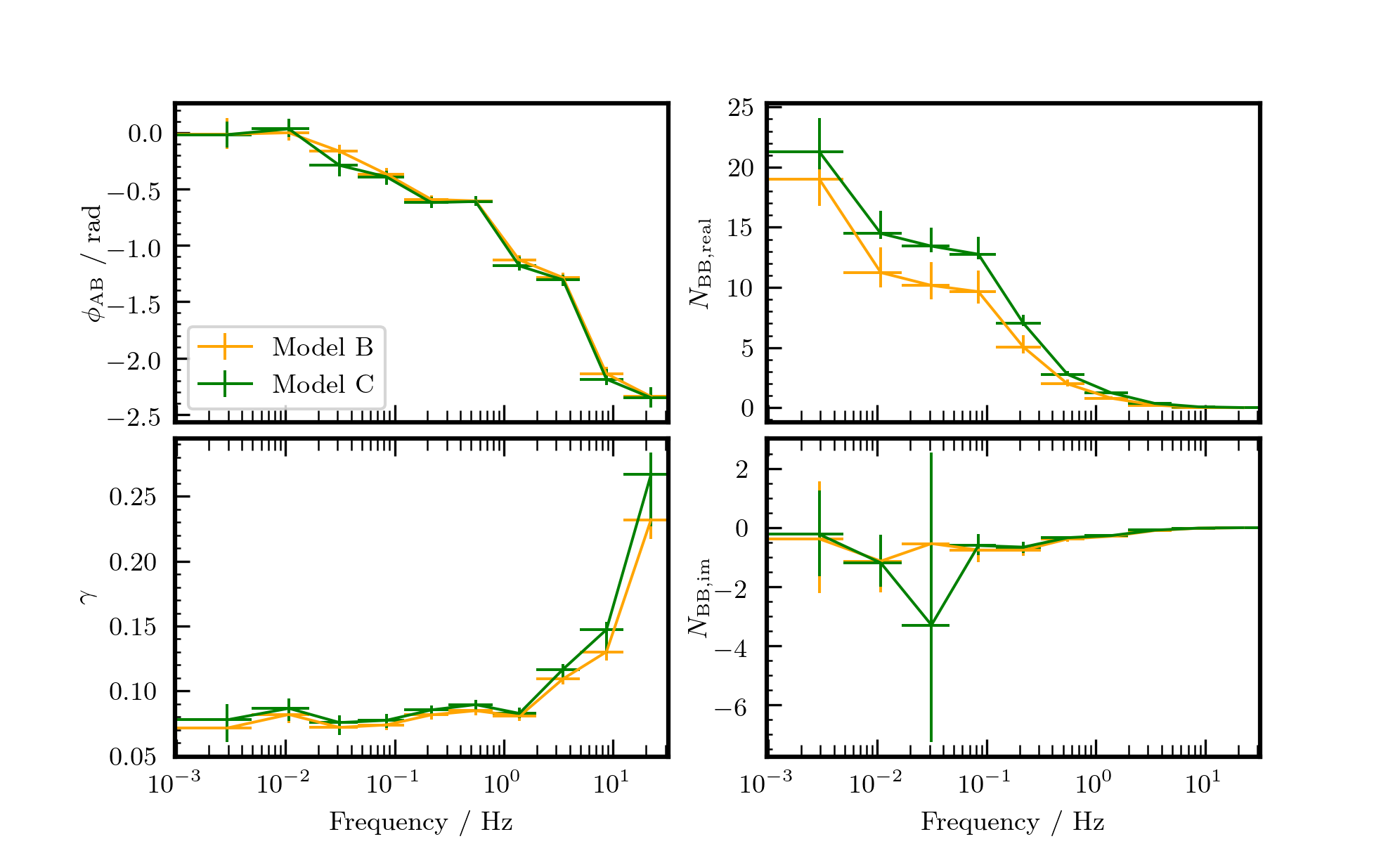
Figure 13: Best fit empirical parameters $\phi_{AB}$ (top left) and $\gamma$ (bottom left); and bbody normalizations for the real (top right) and imaginary parts (bottom right) of the cross spectrum in each frequency band.

Disc variability is represented by the bbody normalization $N_{\rm{BB}}$, which is treated as free parameter for the real and imaginary part of the cross spectrum in each frequency band (i.e. $N_{\rm{BB},\rm{real}}$ is independent of $N_{\rm{BB},\rm{im}}$ for each frequency range). The best fitting values for Models B and C are plotted in Fig. 13. These values are used to calculate the lag and variability amplitude presented in Fig. 11.

References

- Abbott et al. (2023) Abbott R., et al., 2023, Physical Review X, 13, 011048
- Alston et al. (2020) Alston W. N., et al., 2020, Nature Astronomy, 4, 597
- Arévalo & Uttley (2006) Arévalo P., Uttley P., 2006, MNRAS, 367, 801
- Arnaud (1996) Arnaud K. A., 1996, in Jacoby G. H., Barnes J., eds, Astronomical Society of the Pacific Conference Series Vol. 101, Astronomical Data Analysis Software and Systems V. p. 17
- Bambi et al. (2021) Bambi C., et al., 2021, Space Sci. Rev., 217, 65
- Basak et al. (2017) Basak R., Zdziarski A. A., Parker M., Islam N., 2017, MNRAS, 472, 4220
- Belczynski et al. (2021) Belczynski K., Done C., Hagen S., Lasota J. P., Sen K., 2021, arXiv e-prints, p. arXiv:2111.09401
- Beloborodov (2001) Beloborodov A., 2001, Advances in Space Research, 28, 411
- Bendat & Piersol (2000) Bendat J., Piersol A., 2000, Measurement Science and Technology, 11, 1825
- Buisson et al. (2019) Buisson D. J. K., et al., 2019, MNRAS, 490, 1350
- Caballero-García et al. (2018) Caballero-García M. D., Papadakis I. E., Dovčiak M., Bursa M., Epitropakis A., Karas V., Svoboda J., 2018, MNRAS, 480, 2650
- Cackett et al. (2014) Cackett E. M., Zoghbi A., Reynolds C., Fabian A. C., Kara E., Uttley P., Wilkins D. R., 2014, MNRAS, 438, 2980
- Churazov et al. (2001) Churazov E., Gilfanov M., Revnivtsev M., 2001, MNRAS, 321, 759
- Connors et al. (2020) Connors R. M. T., et al., 2020, ApJ, 892, 47
- De Marco et al. (2013) De Marco B., Ponti G., Cappi M., Dadina M., Uttley P., Cackett E. M., Fabian A. C., Miniutti G., 2013, MNRAS, 431, 2441
- Done et al. (2007) Done C., Gierliński M., Kubota A., 2007, A&ARv, 15, 1
- Eardley et al. (1975) Eardley D. M., Lightman A. P., Shapiro S. L., 1975, ApJ, 199, L153
- Fabian & Ross (2010) Fabian A. C., Ross R. R., 2010, Space Sci. Rev., 157, 167
- Fabian et al. (1989) Fabian A. C., Rees M. J., Stella L., White N. E., 1989, MNRAS, 238, 729
- Fabian et al. (2009) Fabian A. C., et al., 2009, Nature, 459, 540
- Feng et al. (2022) Feng M. Z., et al., 2022, ApJ, 934, 47
- Frank et al. (2002) Frank J., King A., Raine D. J., 2002, Accretion Power in Astrophysics: Third Edition. Cambridge University Press
- Galeev et al. (1979) Galeev A. A., Rosner R., Vaiana G. S., 1979, ApJ, 229, 318
- García & Kallman (2010) García J., Kallman T. R., 2010, ApJ, 718, 695
- García et al. (2013a) García J., Dauser T., Reynolds C. S., Kallman T. R., McClintock J. E., Wilms J., Eikmann W., 2013a, ApJ, 768, 146
- García et al. (2013b) García J., Elhoussieny E. E., Bautista M. A., Kallman T. R., 2013b, ApJ, 775, 8
- García et al. (2014a) García J., et al., 2014a, ApJ, 782, 76
- García et al. (2014b) García J. A., McClintock J. E., Steiner J. F., Remillard R. A., Grinberg V., 2014b, ApJ, 794, 73
- García et al. (2015) García J. A., Dauser T., Steiner J. F., McClintock J. E., Keck M. L., Wilms J., 2015, ApJ, 808, L37
- García et al. (2016) García J. A., Fabian A. C., Kallman T. R., Dauser T., Parker M. L., McClintock J. E., Steiner J. F., Wilms J., 2016, MNRAS, 462, 751
- George & Fabian (1991) George I. M., Fabian A. C., 1991, MNRAS, 249, 352
- Gilfanov et al. (2000) Gilfanov M., Churazov E., Revnivtsev M., 2000, MNRAS, 316, 923
- Ingram (2012) Ingram A. R., 2012, PhD thesis, Durham University, UK
- Ingram (2019) Ingram A., 2019, MNRAS, 489, 3927
- Ingram & van der Klis (2013) Ingram A., van der Klis M., 2013, MNRAS, 434, 1476
- Ingram et al. (2019) Ingram A., Mastroserio G., Dauser T., Hovenkamp P., van der Klis M., García J. A., 2019, MNRAS, 488, 324
- Ingram et al. (2022) Ingram A., et al., 2022, MNRAS, 509, 619
- Ingram et al. (2024) Ingram A., et al., 2024, ApJ, 968, 76
- Jiang et al. (2019) Jiang J., et al., 2019, MNRAS, 489, 3436
- Jonker et al. (2021) Jonker P. G., Kaur K., Stone N., Torres M. A. P., 2021, ApJ, 921, 131
- Kara et al. (2016) Kara E., Alston W. N., Fabian A. C., Cackett E. M., Uttley P., Reynolds C. S., Zoghbi A., 2016, MNRAS, 462, 511
- Kara et al. (2019) Kara E., et al., 2019, Nature, 565, 198
- Karpouzas et al. (2020) Karpouzas K., Méndez M., Ribeiro E. M., Altamirano D., Blaes O., García F., 2020, MNRAS, 492, 1399
- Kawamura et al. (2022) Kawamura T., Axelsson M., Done C., Takahashi T., 2022, MNRAS, 511, 536
- Körding & Falcke (2004) Körding E., Falcke H., 2004, A&A, 414, 795
- Kotov et al. (2001) Kotov O., Churazov E., Gilfanov M., 2001, MNRAS, 327, 799
- Krawczynski et al. (2022) Krawczynski H., et al., 2022, Science, 378, 650
- Kylafis et al. (2008) Kylafis N. D., Papadakis I. E., Reig P., Giannios D., Pooley G. G., 2008, A&A, 489, 481
- Lai et al. (2022) Lai E. V., et al., 2022, MNRAS, 512, 2671
- Liu et al. (2023) Liu H., et al., 2023, ApJ, 950, 5
- Lucchini et al. (2022) Lucchini M., Kara E., Mastroserio G., Ingram A., Garcia J., Dauser T., 2022, in AAS/High Energy Astrophysics Division. p. 406.06
- Lyubarskii (1997) Lyubarskii Y. E., 1997, MNRAS, 292, 679
- Mahmoud & Done (2018) Mahmoud R. D., Done C., 2018, MNRAS, 480, 4040
- Markoff et al. (2005) Markoff S., Nowak M. A., Wilms J., 2005, ApJ, 635, 1203
- Mastroserio et al. (2018) Mastroserio G., Ingram A., van der Klis M., 2018, MNRAS, 475, 4027
- Mastroserio et al. (2019) Mastroserio G., Ingram A., van der Klis M., 2019, MNRAS, 488, 348
- Mastroserio et al. (2020) Mastroserio G., Ingram A., van der Klis M., 2020, MNRAS, 498, 4971
- Mastroserio et al. (2021) Mastroserio G., et al., 2021, MNRAS, 507, 55
- Matt & Perola (1992) Matt G., Perola G. C., 1992, MNRAS, 259, 433
- Miller-Jones et al. (2021) Miller-Jones J. C. A., et al., 2021, Science, 371, 1046
- Miniutti & Fabian (2004) Miniutti G., Fabian A. C., 2004, MNRAS, 349, 1435
- Mushtukov et al. (2018) Mushtukov A. A., Ingram A., van der Klis M., 2018, MNRAS, 474, 2259
- Nathan et al. (2024) Nathan E., et al., 2024, MNRAS, 533, 2441
- Novikov & Thorne (1973) Novikov I. D., Thorne K. S., 1973, in Black Holes (Les Astres Occlus). pp 343–450
- Nowak et al. (1999) Nowak M. A., Vaughan B. A., Wilms J., Dove J. B., Begelman M. C., 1999, ApJ, 510, 874
- Parker et al. (2015) Parker M. L., et al., 2015, ApJ, 808, 9
- Poutanen et al. (2018) Poutanen J., Veledina A., Zdziarski A. A., 2018, A&A, 614, A79
- Poutanen et al. (2023) Poutanen J., Veledina A., Beloborodov A. M., 2023, ApJ, 949, L10
- Rapisarda et al. (2016) Rapisarda S., Ingram A., Kalamkar M., van der Klis M., 2016, MNRAS, 462, 4078
- Rapisarda et al. (2017) Rapisarda S., Ingram A., van der Klis M., 2017, MNRAS, 472, 3821
- Revnivtsev et al. (1999) Revnivtsev M., Gilfanov M., Churazov E., 1999, A&A, 347, L23
- Ricketts et al. (2024) Ricketts B., Huppenkothen D., Lucchini M., Ingram A., Mastroserio G., Ho M., Wandelt B., 2024, arXiv e-prints, p. arXiv:2412.10131
- Ross & Fabian (2005) Ross R. R., Fabian A. C., 2005, MNRAS, 358, 211
- Salvesen (2022) Salvesen G., 2022, ApJ, 940, L22
- Shakura & Sunyaev (1973) Shakura N. I., Sunyaev R. A., 1973, A&A, 24, 337
- Shreeram & Ingram (2020) Shreeram S., Ingram A., 2020, MNRAS, 492, 405
- Steiner et al. (2012) Steiner J. F., McClintock J. E., Reid M. J., 2012, ApJ, 745, L7
- Thorne & Price (1975) Thorne K. S., Price R. H., 1975, ApJ, 195, L101
- Tomsick et al. (2014) Tomsick J. A., et al., 2014, ApJ, 780, 78
- Tomsick et al. (2018) Tomsick J. A., et al., 2018, ApJ, 855, 3
- Toor & Seward (1974) Toor A., Seward F. D., 1974, AJ, 79, 995
- Uttley & Malzac (2025) Uttley P., Malzac J., 2025, MNRAS, 536, 3284
- Uttley et al. (2014) Uttley P., Cackett E. M., Fabian A. C., Kara E., Wilkins D. R., 2014, A&ARv, 22, 72
- Veledina et al. (2023) Veledina A., et al., 2023, ApJ, 958, L16
- Vikhlinin et al. (1994) Vikhlinin A., Churazov E., Gilfanov M., 1994, A&A, 287, 73
- Walton et al. (2016) Walton D. J., et al., 2016, ApJ, 826, 87
- Wang et al. (2021) Wang J., et al., 2021, ApJ, 910, L3
- Wang et al. (2022) Wang J., et al., 2022, ApJ, 930, 18
- Wilkinson & Uttley (2009) Wilkinson T., Uttley P., 2009, MNRAS, 397, 666
- Wilms et al. (2000) Wilms J., Allen A., McCray R., 2000, ApJ, 542, 914
- Zdziarski et al. (1996) Zdziarski A. A., Johnson W. N., Magdziarz P., 1996, MNRAS, 283, 193
- Zdziarski et al. (2021) Zdziarski A. A., De Marco B., Szanecki M., Niedźwiecki A., Markowitz A., 2021, ApJ, 906, 69
- Zdziarski et al. (2022) Zdziarski A. A., You B., Szanecki M., Li X.-B., Ge M., 2022, ApJ, 928, 11
- Zhang et al. (1995) Zhang W., Jahoda K., Swank J. H., Morgan E. H., Giles A. B., 1995, ApJ, 449, 930
- Zhao et al. (2021) Zhao X., et al., 2021, ApJ, 908, 117
- van der Klis (1989) van der Klis M., 1989, in Ögelman H., van den Heuvel E. P. J., eds, NATO Advanced Science Institutes (ASI) Series C Vol. 262, NATO Advanced Science Institutes (ASI) Series C. p. 27
- van der Klis et al. (1987) van der Klis M., Hasinger G., Stella L., Langmeier A., van Paradijs J., Lewin W. H. G., 1987, ApJ, 319, L13