Conservative, pressure-equilibrium-preserving discontinuous Galerkin method for compressible, multicomponent flows

Abstract

This paper concerns preservation of velocity and pressure equilibria in smooth, compressible, multicomponent flows in the inviscid limit. First, we derive the velocity-equilibrium and pressure-equilibrium conditions of a standard discontinuous Galerkin method that discretizes the conservative form of the compressible, multicomponent Euler equations. We show that under certain constraints on the numerical flux, the scheme is velocity-equilibrium-preserving. However, standard discontinuous Galerkin schemes are not pressure-equilibrium-preserving. Therefore, we introduce a discontinuous Galerkin method that discretizes the pressure-evolution equation in place of the total-energy conservation equation. Semidiscrete conservation of total energy, which would otherwise be lost, is restored via the correction terms of Abgrall [1] and Abgrall et al. [2]. Since the addition of the correction terms prevents exact preservation of pressure and velocity equilibria, we propose modifications that then lead to a velocity-equilibrium-preserving, pressure-equilibrium-preserving, and (semidiscretely) energy-conservative discontinuous Galerkin scheme, although there are certain tradeoffs. Additional extensions are also introduced. We apply the developed scheme to smooth, interfacial flows involving mixtures of thermally perfect gases initially in pressure and velocity equilibria to demonstrate its performance in one, two, and three spatial dimensions.

1 Introduction

Compressible, multicomponent flows are relevant to many engineering applications and physical phenomena, including propulsion, atmospheric entry, and pollutant formation. However, robust and accurate simulation of such flows remains challenging. For instance, a well-known, long-standing issue is the failure of conventional conservative numerical schemes to preserve pressure equilibrium at fluid interfaces in the inviscid limit, leading to spurious pressure oscillations that can then cause noticeable errors and even solver divergence. Note that pressure-equilibrium preservation corresponds to the ability to maintain uniform pressure under initially constant velocity and pressure in inviscid flows, and velocity equilibrium is typically implicitly assumed when referring to pressure equilibrium. These spurious pressure oscillations arise when the specific heat ratio of the mixture is no longer constant, which can occur even in the case of a monocomponent thermally perfect gas or a mixture of calorically perfect gases. Although the addition of numerical dissipation via, for instance, artificial viscosity or limiting can mitigate these oscillations and help prevent solver divergence, these stabilization techniques do not guarantee pressure-equilibrium preservation and will still often generate errors in pressure [3]. In addition, such techniques can introduce excessive dissipation (to the detriment of accuracy) in complex flow problems. To address this difficulty, many quasi-conservative schemes (i.e., schemes that sacrifice discrete conservation of mass and/or total energy) have been developed. One example is the double-flux method [4], in which the thermodynamics are locally frozen to mimic the calorically perfect, single-species setting. Alternatively, the pressure-evolution equation can be solved in place of the total-energy equation [5, 6, 7, 8]. These two quasi-conservative approaches mathematically guarantee preservation of pressure equilibrium at the cost of total-energy conservation. However, loss of conservation is often considered to be unsatisfactory, especially at shocks. Hybrid strategies that switch between pressure-equilibrium-preserving (but quasi-conservative) and conservative (but non-pressure-equilibrium-preserving) schemes have been proposed [9, 10, 11, 12, 13].

To prevent loss of conservation, recent efforts in the computational fluid dynamics (CFD) community have focused on conservative schemes that mitigate spurious pressure oscillations without relying on artificial viscosity or limiting. Some of these approaches belong to the family of numerical schemes known as discontinuous Galerkin (DG) methods [14, 15, 16, 17, 18], which have gained considerable attention due to high-order accuracy, geometric flexibility, amenability to modern computing systems, and other advantages [19]. A number of studies [20, 21, 3] have found that the type of integration (i.e., colocation or overintegration) can have a noticeable effect on the magnitude of spurious pressure oscillations. In addition, projecting the pressure onto the finite element test space prior to evaluating the flux (akin to reconstruction of the primitive variables in finite-volume schemes [12, 22]) can attenuate the pressure oscillations [23, 20, 21, 3]. Note that these methods do not mathematically guarantee preservation of pressure equilibrium. In contrast, Fujiwara et al. [24] recently introduced a fully conservative finite volume scheme for the compressible, multicomponent Euler equations that provably maintains pressure equilibrium. The key ingredient was the derivation of a discrete pressure-equilibrium condition that informed the development of a provably pressure-equilibrium-preserving numerical flux, albeit with the caveat that calorically perfect gas mixtures are assumed (i.e., each species has a constant specific heat ratio). Terashima et al. [25] then extended this approach to real fluids modeled with a cubic equation of state, although the more complicated relationship between pressure and internal energy results in an approximately pressure-equilibrium-preserving numerical flux, where second-order spatial errors with respect to exact pressure equilibrium were reported. To the best of our knowledge, even in the simpler (but still complex) case of mixtures of thermally perfect gases (i.e., each species has a temperature-dependent specific heat ratio), which are considered in this work, conservative schemes that mathematically preserve pressure equilibrium have remained elusive. The primary objective of the present study is to address this gap.

We first extend some of the analysis in [24] and show that a standard DG discretization of the conservative form of the multicomponent Euler equations is velocity-equilibrium-preserving but not pressure-equilibrium-preserving. We then introduce a pressure-based DG method (i.e., total energy is replaced with pressure as a state variable) in which semidiscrete total-energy conservation is restored via the conservative, high-order, elementwise correction terms of Abgrall [1] and Abgrall et al. [2]. These correction terms enable semidiscrete satisfaction of auxiliary transport equations (here, the total-energy equation) in an integral sense. Note that it may seem more natural to retain total energy as a state variable and design the correction terms to additionally satisfy the pressure-evolution equation. However, pressure equilibrium is essentially a pointwise condition, whereas the correction terms only guarantee integral satisfaction of the auxiliary transport equation(s). Entropy-conservative/entropy-stable DG schemes have been constructed using these correction terms (or similar forms) without relying on SBP operators or entropy-conservative/entropy-stable numerical fluxes [1, 26, 27, 28, 29]. The correction terms have also been employed to enforce conservation of total energy while treating entropy density as a state variable [30]. Here, the difficulties associated with devising a provably pressure-equilibrium-preserving numerical flux for non-calorically-perfect gases can be circumvented using the correction terms, although a distinct set of challenges is also introduced. For instance, although a standard pressure-based DG method (i.e., without the correction terms) can exactly maintain pressure and velocity equilibria, the addition of the correction terms results in loss of this property. Furthermore, for a given element, the correction terms are only valid if the state inside the element is non-uniform, thus ignoring the case of elementwise-constant solutions with inter-element jumps. The correction terms also fail to preserve zero species concentrations, which can be especially detrimental if chemical reactions are considered. We develop modifications to the correction terms that enable exact preservation of pressure equilibrium, velocity equilibrium, and zero species concentrations (while maintaining semidiscrete total-energy conservation) in multicomponent flows, although it should be noted that there are certain tradeoffs. In addition, we propose combining the elementwise correction terms with face-based corrections of the form presented in [30] in order to account for elementwise-constant solutions with inter-element jumps. Detailed comparisons of the correction terms with and without the modifications are performed. In this study, we target smooth, interfacial flows initially in pressure and velocity equilibria, as in [24] and [25], and mixtures of thermally perfect gases. No artificial viscosity or limiting is applied in the considered test cases. The eventual goal is to account for flows with or without discontinuities involving real-fluid mixtures, which are even more susceptible to large-scale spurious pressure oscillations and solver divergence due to the additional thermodynamic nonlinearities. This will be the subject of future work.

Note that the proposed formulation is similar in spirit to a recent ADER-DG method developed by Gaburro et al. [13], which also treats pressure as a state variable and incorporates total-energy-based corrections. However, there are some key differences. First, the total-energy corrections in [13] are of a subcell finite-volume type, distinct from the correction terms employed in this study. In addition, the ADER-DG method in [13] only applies the corrections at shocks, which are detected using a shock sensor, such that total energy is not conserved everywhere in the domain. It should be noted that total-energy conservation is most critical at shocks [5, 6, 31, 32] and may not need to be satisfied elsewhere to obtain accurate results. Finally, the subcell finite-volume-type corrections, if applied to a constant-pressure fluid interface, may not preserve pressure equilibrium. Regardless, the method in [13] was used to obtain very encouraging results in discontinuous multi-material flows involving calorically perfect gases. Here, we specifically focus on recovering total-energy conservation everywhere in the domain; a detailed investigation of whether total-energy conservation can be sacrificed away from shocks, especially in practical problems, is outside the scope of the current study but may be pursued in the future.

The remainder of this paper is organized as follows. Section 2 briefly summarizes the conservative form of the governing equations and the corresponding DG discretization. The pressure-based formulation, correction terms, and proposed modifications are introduced in the following section. Results for a variety of smooth, interfacial flow problems initially in pressure and velocity equilibria are given in Section 4, wherein curved elements are also considered. The paper concludes with some broader discussion and final remarks.

2 Compressible, multicomponent Euler equations: Total-energy-based formulation

Before discussing the pressure-based formulation, we begin with the conservative form of the compressible, multicomponent Euler equations:

$$\partial_{t}\bm{y}+\nabla\cdot\bm{\mathcal{F}}\left(\bm{y}\right)=0,$$ (2.1)

where $t$ is the time, $\bm{y}$ is the vector of $m$ state variables, and $\bm{\mathcal{F}}$ is the convective flux. The physical coordinates are denoted by $x=(x_{1},\ldots,x_{d})$, where $d$ is the number of spatial dimensions. The state vector is expanded as

$$\bm{y}=\left(\rho v_{1},\ldots,\rho v_{d},\rho e_{t},C_{1},\ldots,C_{n_{s}}\right)^{T},$$ (2.2)

where $\rho$ is the density, $\bm{v}=\left(v_{1},\ldots,v_{d}\right)$ is the velocity vector, $e_{t}$ is the specific total energy, and $C_{i}$ is the molar concentration of the $i$th (out of $n_{s}$) species. Note that the first $d$ components of $\bm{y}$ correspond to momentum, the $\left(d+1\right)$th component corresponds to energy, and the last $n_{s}$ components correspond to species concentrations. The density is computed from the species concentrations as

$$\rho=\sum_{i=1}^{n_{s}}\rho_{i}=\sum_{i=1}^{n_{s}}W_{i}C_{i},$$

where $\rho_{i}$ and $W_{i}$ are the partial density and molar mass, respectively, of the $i$th species. Throughout this work, we assume $\rho>0$ (i.e., no vacuum). The mass and mole fractions of the $i$th species are given by

$$Y_{i}=\frac{\rho_{i}}{\rho},\quad X_{i}=\frac{C_{i}}{\sum_{i=1}^{n_{s}}C_{i}},$$

and the specific total energy is expanded as

$$e_{t}=u+\frac{1}{2}\sum_{k=1}^{d}v_{k}v_{k},$$

where $u=\sum_{i=1}^{n_{s}}Y_{i}u_{i}$ is the mixture-averaged specific internal energy. Under the assumption of thermally perfect gases, $u_{i}$ is defined as [33]

$$u_{i}=h_{i}-R_{i}T=h_{\mathrm{ref},i}+\int_{T_{\mathrm{ref}}}^{T}c_{p,i}(\tau)d\tau-R_{i}T,$$

where $h_{i}$ is the mass-specific enthalpy of the $i$th species, $R_{i}=R^{0}/W_{i}$ (with $R^{0}$ denoting the universal gas constant), $T$ is the temperature, $T_{\mathrm{ref}}=298.15\>\mathrm{K}$ is the reference temperature, $h_{\mathrm{ref},i}$ is the reference-state species formation enthalpy, and $c_{p,i}$ is the mass-specific heat capacity at constant pressure of the $i$th species. $c_{p,i}$ is computed from an $n_{p}$-order polynomial as

$$c_{p,i}=\sum_{k=0}^{n_{p}}a_{ik}T^{k},$$ (2.3)

based on the NASA thermodynamic fits [34, 35].

The $k$th spatial component of the convective flux is given by

$$\bm{\mathcal{F}}_{k}\left(y\right)=\left(\rho v_{k}v_{1}+P\delta_{k1},\ldots,\rho v_{k}v_{d}+P\delta_{kd},v_{k}\left(\rho e_{t}+P\right),v_{k}C_{1},\ldots,v_{k}C_{n_{s}}\right)^{T},$$ (2.4)

where $P$ is the pressure, which is computed from the ideal-gas law:

$$P=R^{0}T\sum_{i}C_{i}=\rho RT.$$ (2.5)

$R=R^{0}/\overline{W}$ is the specific gas constant, where $\overline{W}=\rho/\sum_{i}^{n_{s}}C_{i}$ is the molar mass of the mixture.

2.1 Discontinuous Galerkin discretization

Let $\Omega$ denote the computational domain partitioned by $\mathcal{T}$, which consists of cells $\kappa$ with boundaries $\partial\kappa$. Let $\mathcal{E}$ denote the set of interfaces $\epsilon$, consisting of the interior interfaces,

$$\epsilon_{\mathcal{I}}\in\mathcal{E_{I}}=\left\{\epsilon_{\mathcal{I}}\in\mathcal{E}\,\middle|\,\epsilon_{\mathcal{I}}\cap\partial\Omega=\emptyset\right\},$$

and boundary interfaces,

$$\epsilon_{\partial}\in\mathcal{E}_{\partial}=\left\{\epsilon_{\partial}\in\mathcal{E}\,\middle|\,\epsilon_{\partial}\subset\partial\Omega\right\}.$$

At interior interfaces, there exist $\kappa^{+}$ and $\kappa^{-}$ such that $\epsilon_{\mathcal{I}}=\partial\kappa^{+}\cap\partial\kappa^{-}$. $n^{+}$ and $n^{-}$ denote the outward facing normals of $\kappa^{+}$ and $\kappa^{-}$, respectively. Let $V_{h}^{p}$ denote the space of test functions,

$$V_{h}^{p} = \left\{\bm{\mathfrak{v}}\in\left[L^{2}\left(\Omega\right)\right]^{m}\,\middle|\,\forall\kappa\in\mathcal{T},\left.\bm{\mathfrak{v}}\right|_{\kappa}\in\left[\mathcal{P}_{p}(\kappa)\right]^{m}\right\},$$ (2.6)

where $\mathcal{P}_{p}(\kappa)$ is a space of polynomial functions of degree no greater than $p$ in $\kappa$.

The semi-discrete form of Equation (2.1) is as follows: find $\bm{y}\in V_{h}^{p}$ such that

$$\sum_{\kappa\in\mathcal{T}}\left(\partial_{t}\bm{y},\bm{\mathfrak{v}}\right)_{\kappa}-\sum_{\kappa\in\mathcal{T}}\left(\bm{\mathcal{F}}\left(\bm{y}\right),\nabla\bm{\mathfrak{v}}\right)_{\kappa}+\sum_{\epsilon\in\mathcal{E}}\left(\bm{\mathcal{F}}^{\dagger}\left(\bm{y},\bm{n}\right),\left\llbracket\bm{\mathfrak{v}}\right\rrbracket\right)_{\mathcal{E}}=0\qquad\forall\>\bm{\mathfrak{v}}\in V_{h}^{p},$$ (2.7)

where $\left(\cdot,\cdot\right)$ denotes the inner product, $\bm{\mathcal{F}}^{\dagger}\left(y,n\right)$ is the flux function, and $\left\llbracket\cdot\right\rrbracket$ is the jump operator. At interior interfaces, $\left\llbracket\bm{\mathfrak{v}}\right\rrbracket=\bm{\mathfrak{v}}^{+}-\bm{\mathfrak{v}}^{-}$ and $\bm{\mathcal{F}}^{\dagger}\left(\bm{y},\bm{n}\right)=\bm{\mathcal{F}}^{\dagger}\left(\bm{y}^{+},\bm{y}^{-},\bm{n}\right)$, where $\bm{\mathcal{F}}^{\dagger}\left(\bm{y}^{+},\bm{y}^{-},\bm{n}\right)$ is a numerical flux. Throughout this work, we use the local Lax-Friedrichs numerical flux,

$$\bm{\mathcal{F}}^{\dagger}\left(\bm{y}^{+},\bm{y}^{-},\bm{n}\right) =\left\{\!\!\left\{\bm{\mathcal{F}}\left(\bm{y}\right)\right\}\!\!\right\}\cdot\bm{n}+\frac{1}{2}\lambda\left\llbracket\bm{y}\right\rrbracket,$$ (2.8)

where $\left\{\!\!\left\{\cdot\right\}\!\!\right\}$ denotes the average operator and $\lambda$ is an estimate of the maximum wave speed across $\bm{y}^{+}$ and $\bm{y}^{-}$. More information on boundary conditions can be found in [20, 36]. The element-local solution, $\left.\bm{y}\right|_{\kappa}$, can be expanded as (dropping the $\left.\left(\cdot\right)\right|_{\kappa}$ notation for brevity)

$$\bm{y}=\sum_{j=1}^{n_{b}}\widehat{\bm{y}}_{j}\phi_{j},$$

where $\widehat{\bm{y}}_{j}$ is the $j$th polynomial coefficient, $\phi_{j}$ is the $j$th basis function, and $n_{b}$ is the number of basis functions. A nodal basis is employed in this work. In element-local integral form, we have (assuming all interior faces)

$$\int_{\kappa}\phi_{i}\partial_{t}\bm{y}dx-\int_{\kappa}\nabla\phi_{i}\cdot\bm{\mathcal{F}}\left(\bm{y}\right)dx+\oint_{\partial\kappa}\phi_{i}\bm{\mathcal{F}}^{\dagger}\left(\bm{y}^{+},\bm{y}^{-},\bm{n}\right)ds=0,\quad i=1,\ldots,n_{b}.$$ (2.9)

Introducing the mass matrix, $\mathcal{M}_{ij}=\int_{\kappa}\phi_{i}\phi_{j}dx,$ we can rewrite Equation (2.9) as

$$\bm{\mathcal{M}}d_{t}\widehat{\bm{y}}-\int_{\kappa}\nabla\bm{\Phi}\cdot\bm{\mathcal{F}}\left(\bm{y}\right)dx+\oint_{\partial\kappa}\bm{\Phi}\bm{\mathcal{F}}^{\dagger}\left(\bm{y}^{+},\bm{y}^{-},\bm{n}\right)ds=0,$$ (2.10)

where $\widehat{\bm{y}}=\left[\widehat{\bm{y}}_{1},\ldots,\widehat{\bm{y}}_{n_{b}}\right]$ is the vector of polynomial coefficients and $\bm{\Phi}=\left[\phi_{1},\ldots,\phi_{n_{b}}\right]^{T}$ is the vector of basis functions. Left-multiplying both sides by $\bm{\Phi}^{T}\bm{\mathcal{M}}^{-1}$ yields

$$\partial_{t}\bm{y}-\bm{\Phi}^{T}\bm{\mathcal{M}}^{-1}\int_{\kappa}\nabla\bm{\Phi}\cdot\bm{\mathcal{F}}\left(\bm{y}\right)dx+\bm{\Phi}^{T}\bm{\mathcal{M}}^{-1}\oint_{\partial\kappa}\bm{\Phi}\bm{\mathcal{F}}^{\dagger}\left(\bm{y}^{+},\bm{y}^{-},\bm{n}\right)ds=0,$$ (2.11)

which represents the temporal evolution of $\bm{y}\left(\bm{x},t\right)$. Here, it is implicitly assumed that, for example, $\bm{\mathcal{M}}d_{t}\widehat{\bm{y}}$ represents the matrix-vector product between the mass matrix and each of the $m$ components of $d_{t}\widehat{\bm{y}}$ (and similarly for related operations).

2.1.1 Velocity-equilibrium preservation

We examine whether the DG discretization in the previous subsection exactly preserves velocity equilibrium. This represents an extension of the analysis by Fujiwara et al. [24] to DG schemes and a generalization of that by [21], who focused on discontinuous interfaces, to smooth interfaces. The velocity evolution equation is given by [24]

$$\partial_{t}\bm{v}=\frac{1}{\rho}\partial_{t}\left(\rho\bm{v}\right)-\frac{\bm{v}}{\rho}\partial_{t}\rho,$$ (2.12)

where $\partial_{t}\rho=\sum_{i}W_{i}\partial_{t}C_{i}$. For simplicity, we focus on the one-dimensional case, but extensions to $d>1$ are straightforward.

Lemma 1.

In the case of constant pressure $(P=P_{0})$ and velocity $\left(\bm{v}=\bm{v}_{0}\right)$, the DG discretization (2.9) preserves velocity equilibrium (i.e., $\partial_{t}v=0$ necessarily) if and only if the numerical flux satisfies

$$P_{0}\oint_{\partial\kappa}\bm{\Phi}\cdot ndx-\oint_{\partial\kappa}\bm{\Phi}\mathcal{F}_{\rho v}^{\dagger}\left(\bm{y}^{+},\bm{y}^{-},n\right)ds+v_{0}\oint_{\partial\kappa}\bm{\Phi}\sum_{i}W_{i}\mathcal{F}_{C_{i}}^{\dagger}\left(\bm{y}^{+},\bm{y}^{-},n\right)ds=0,$$ (2.13)

where $\mathcal{F}_{\rho v}^{\dagger}\left(\bm{y}^{+},\bm{y}^{-},n\right)$ is the momentum component of the numerical flux and $\mathcal{F}_{C_{i}}^{\dagger}\left(\bm{y}^{+},\bm{y}^{-},n\right)$ is the component corresponding to the $i$th species concentration,.

Proof.

Substituting the momentum and concentration components of the temporal evolution of the local solution (2.11) into Equation (2.12) yields

$$\partial_{t}v= \bm{\Phi}^{T}\bm{\mathcal{M}}^{-1}\left(\frac{1}{\rho}\left[\int_{\kappa}\partial_{x}\bm{\Phi}\begin{pmatrix}\rho v^{2}+P\end{pmatrix}dx-\oint_{\partial\kappa}\bm{\Phi}\mathcal{F}_{\rho v}^{\dagger}\left(\bm{y}^{+},\bm{y}^{-},n\right)ds\right]\right.$$

$$\left.-\frac{v}{\rho}\left[\int_{\kappa}\partial_{x}\bm{\Phi}\begin{pmatrix}\rho v\end{pmatrix}dx-\oint_{\partial\kappa}\bm{\Phi}\sum_{i}W_{i}\mathcal{F}_{C_{i}}^{\dagger}\left(\bm{y}^{+},\bm{y}^{-},n\right)ds\right]\right)$$

$$= \bm{\Phi}^{T}\bm{\mathcal{M}}^{-1}\Biggl{(}\frac{1}{\rho}\left[v_{0}^{2}\int_{\kappa}\partial_{x}\bm{\Phi}\rho dx+P_{0}\int_{\kappa}\partial_{x}\bm{\Phi}dx-\oint_{\partial\kappa}\bm{\Phi}\mathcal{F}_{\rho v}^{\dagger}\left(\bm{y}^{+},\bm{y}^{-},n\right)ds\right]$$

$$-\frac{v_{0}}{\rho}\left[v_{0}\int_{\kappa}\partial_{x}\bm{\Phi}\cdot\begin{pmatrix}\rho\end{pmatrix}dx-\oint_{\partial\kappa}\bm{\Phi}\sum_{i}W_{i}\mathcal{F}_{C_{i}}^{\dagger}\left(\bm{y}^{+},\bm{y}^{-},n\right)ds\right]\Biggr{)}$$

$$= \bm{\Phi}^{T}\bm{\mathcal{M}}^{-1}\left(\frac{P_{0}}{\rho}\oint_{\partial\kappa}\bm{\Phi}\cdot ndx-\frac{1}{\rho}\oint_{\partial\kappa}\bm{\Phi}\mathcal{F}_{\rho v}^{\dagger}\left(\bm{y}^{+},\bm{y}^{-},n\right)ds+\frac{v_{0}}{\rho}\oint_{\partial\kappa}\bm{\Phi}\sum_{i}W_{i}\mathcal{F}_{C_{i}}^{\dagger}\left(\bm{y}^{+},\bm{y}^{-},n\right)ds\right),$$

where the last line assumes sufficiently accurate numerical integration. Clearly, if (2.13) is satisfied, the RHS vanishes and $\partial_{t}v=0$. Next, we consider the reverse. Since $\left\{\phi_{1},\ldots,\phi_{n_{b}}\right\}$ forms a basis of $\mathcal{P}_{p}(\kappa)$, $\partial_{t}v=0$ requires

$$\bm{\mathcal{M}}^{-1}\left(\frac{P_{0}}{\rho}\oint_{\partial\kappa}\bm{\Phi}\cdot ndx-\frac{1}{\rho}\oint_{\partial\kappa}\bm{\Phi}\mathcal{F}_{\rho v}^{\dagger}\left(\bm{y}^{+},\bm{y}^{-},n\right)ds+\frac{v_{0}}{\rho}\oint_{\partial\kappa}\bm{\Phi}\sum_{i}W_{i}\mathcal{F}_{C_{i}}^{\dagger}\left(\bm{y}^{+},\bm{y}^{-},n\right)ds\right)=0,$$

which implies that the quantity inside the parentheses is zero because the mass matrix is nonsingular. Therefore, (2.13) must be satisfied. ∎

Remark 2.

The Lax-Friedrichs flux (2.8) satisfies (2.13). To show this, we substitute (2.8) into (2.13), yielding

$$\frac{P_{0}}{\rho}\oint_{\partial\kappa}\bm{\Phi}\cdot ndx-\frac{1}{\rho}\oint_{\partial\kappa}\bm{\Phi}\left[v_{0}^{2}\left\{\!\!\left\{\rho\right\}\!\!\right\}\cdot n+P_{0}\cdot n+\frac{v_{0}}{2}\lambda\left\llbracket\rho\right\rrbracket\right]ds+\frac{v_{0}}{\rho}\oint_{\partial\kappa}\bm{\Phi}\left[v_{0}\left\{\!\!\left\{\rho\right\}\!\!\right\}\cdot n+\frac{1}{2}\lambda\left\llbracket\rho\right\rrbracket\right]ds=0$$

since all terms on the LHS cancel out. Other numerical fluxes, such as the HLLC flux [37], also satisfy (2.13).

Remark 3.

The above analysis focuses on the semidiscrete setting. For certain time integrators, it is straightforward to show fully discrete preservation of velocity equilibrium. For example, letting $\left(\cdot\right)^{n}$ denote the $n$th time step, the Forward Euler scheme combined with the Lax-Friedrichs numerical flux gives

$$\left(\rho\right)^{n+1} =\left(\rho\right)^{n}+\bm{\Phi}^{T}\bm{\mathcal{M}}^{-1}\Delta t\left[\int_{\kappa}\partial_{x}\bm{\Phi}\begin{pmatrix}\rho v\end{pmatrix}dx-\oint_{\partial\kappa}\bm{\Phi}\sum_{i}W_{i}\mathcal{F}_{C_{i}}^{\dagger}\left(\bm{y}^{+},\bm{y}^{-},n\right)ds\right]^{n}$$

$$=\left(\rho\right)^{n}+\bm{\Phi}^{T}\bm{\mathcal{M}}^{-1}\Delta t\left[v_{0}\int_{\kappa}\partial_{x}\bm{\Phi}\rho dx-\oint_{\partial\kappa}\bm{\Phi}\sum_{i}W_{i}\mathcal{F}_{C_{i}}^{\dagger}\left(\bm{y}^{+},\bm{y}^{-},n\right)ds\right]^{n}$$

and

$$\left(\rho v\right)^{n+1} =\left(\rho v\right)^{n}+\bm{\Phi}^{T}\bm{\mathcal{M}}^{-1}\Delta t\left[\int_{\kappa}\partial_{x}\bm{\Phi}\begin{pmatrix}\rho v^{2}+P\end{pmatrix}dx-\oint_{\partial\kappa}\bm{\Phi}\mathcal{F}_{\rho v}^{\dagger}\left(\bm{y}^{+},\bm{y}^{-},n\right)ds\right]^{n}$$

$$=\left(\rho v\right)^{n}+\bm{\Phi}^{T}\bm{\mathcal{M}}^{-1}\Delta t\left[v_{0}^{2}\int_{\kappa}\partial_{x}\bm{\Phi}\rho dx+P_{0}\oint_{\partial\kappa}\bm{\Phi}\cdot ndx-\oint_{\partial\kappa}\bm{\Phi}\mathcal{F}_{\rho v}^{\dagger}\left(\bm{y}^{+},\bm{y}^{-},n\right)ds\right]^{n}.$$

Assuming (2.13) holds, we can rewrite $\left(\rho v\right)^{n+1}$ as

$$\left(\rho v\right)^{n+1} =\left(\rho v\right)^{n}+\bm{\Phi}^{T}\bm{\mathcal{M}}^{-1}\Delta t\left[v_{0}^{2}\int_{\kappa}\partial_{x}\bm{\Phi}\rho dx-v_{0}\oint_{\partial\kappa}\bm{\Phi}\sum_{i}W_{i}\mathcal{F}_{C_{i}}^{\dagger}\left(\bm{y}^{+},\bm{y}^{-},n\right)ds\right]^{n}$$

$$=v_{0}\left(\rho\right)^{n}+\bm{\Phi}^{T}\bm{\mathcal{M}}^{-1}\Delta tv_{0}\left[v_{0}\int_{\kappa}\partial_{x}\bm{\Phi}\rho dx-\oint_{\partial\kappa}\bm{\Phi}\sum_{i}W_{i}\mathcal{F}_{C_{i}}^{\dagger}\left(\bm{y}^{+},\bm{y}^{-},n\right)ds\right]^{n}$$

$$=v_{0}\left(\rho\right)^{n+1}.$$

Therefore,

$$v^{n+1}=\frac{\left(\rho v\right)^{n+1}}{\left(\rho\right)^{n+1}}=\frac{v_{0}\left(\rho\right)^{n+1}}{\left(\rho\right)^{n+1}}=v_{0}.$$

This result directly extends to strong-stability-preserving Runge-Kutta (SSPRK) schemes [38], which can be expressed as convex combinations of Forward Euler steps.

Remark 4.

In the above analysis, it is assumed that $\int_{\kappa}\partial_{x}\bm{\Phi}Pdx$ is exactly integrated (i.e., $\int_{\kappa}\partial_{x}\bm{\Phi}Pdx$ is evaluated to be equal to $P_{0}\int_{\kappa}\partial_{x}\bm{\Phi}dx=P_{0}\oint_{\partial\kappa}\bm{\Phi}\cdot ndx$). However, with standard overintegration, this will often not be the case due to the nonlinear relationship between pressure and internal energy. Assuming a nodal basis and the nodal values of pressure to be $P_{0}$, colocated integration, as well as an overintegration strategy wherein pressure is projected onto $\mathcal{P}_{p}(\kappa)$ in a particular manner, $\int_{\kappa}\partial_{x}\bm{\Phi}Pdx$ will be exactly integrated. See [20, 21] for additional discussion. Regardless, failure to additionally preserve pressure equilibrium, which will be demonstrated next, will eventually disturb velocity equilibrium.

Remark 5.

The above analysis holds regardless of the thermodynamic model (e.g., calorically perfect, thermally perfect, non-ideal, etc.).

2.1.2 Pressure-equilibrium preservation

We now turn to pressure-equilibrium preservation. With $\rho u=\rho u\left(P,C_{1},\ldots,C_{n_{s}}\right)$, the pressure-evolution equation can be written in terms of the conservative variables as [24]

$$\partial_{t}P=\left(\frac{\partial\rho u}{\partial P}\right)_{C_{i}}^{-1}\left[\partial_{t}\left(\rho e_{t}\right)-v\partial_{t}\left(\rho v\right)+\frac{v^{2}}{2}\partial_{t}\rho-\sum_{i}\left(\frac{\partial\rho u}{\partial C_{i}}\right)_{P,C_{j}\neq i}\partial_{t}C_{i}\right].$$ (2.14)

Proposition 6.

In the case of constant pressure $(P=P_{0})$ and velocity $\left(v=v_{0}\right)$, the DG discretization (2.9) preserves pressure equilibrium (i.e., $\partial_{t}P=0$ necessarily) if and only if the condition

$$v_{0}\int_{\kappa}\partial_{x}\bm{\Phi}\rho udx-\oint_{\partial\kappa}\bm{\Phi}\mathcal{F}_{\rho e_{t}}^{\dagger}\left(\bm{y}^{+},\bm{y}^{-},n\right)ds+v_{0}\oint_{\partial\kappa}\bm{\Phi}\mathcal{F}_{\rho v}^{\dagger}\left(\bm{y}^{+},\bm{y}^{-},n\right)ds$$ (2.15)

$$-\frac{v_{0}^{2}}{2}\oint_{\partial\kappa}\bm{\Phi}\sum_{i}W_{i}\mathcal{F}_{C_{i}}^{\dagger}\left(\bm{y}^{+},\bm{y}^{-},n\right)ds=\sum_{i}\left(\frac{\partial\rho u}{\partial\rho_{i}}\right)_{P,\rho_{j}\neq i}\left[v_{0}\int_{\kappa}\partial_{x}\bm{\Phi}\rho_{i}dx-\oint_{\partial\kappa}\bm{\Phi}W_{i}\mathcal{F}_{C_{i}}^{\dagger}\left(\bm{y}^{+},\bm{y}^{-},n\right)ds\right]$$

is satisfied, where $\mathcal{F}_{\rho e_{t}}^{\dagger}\left(y^{+},y^{-},n\right)$ is the total-energy component of the numerical flux.

Proof.

Substituting the temporal evolution of the local solution (2.11) into Equation (2.14) yields

$$\frac{\partial P}{\partial t}= \bm{\Phi}^{T}\bm{\mathcal{M}}^{-1}\left(\frac{\partial\rho u}{\partial P}\right)_{C_{i}}^{-1}\Biggl{\{}v_{0}\int_{\kappa}\partial_{x}\bm{\Phi}\rho udx-\oint_{\partial\kappa}\bm{\Phi}\mathcal{F}_{\rho e_{t}}^{\dagger}\left(\bm{y}^{+},\bm{y}^{-},n\right)ds$$

$$+v_{0}\oint_{\partial\kappa}\bm{\Phi}\mathcal{F}_{\rho v}^{\dagger}\left(\bm{y}^{+},\bm{y}^{-},n\right)ds-\frac{v_{0}^{2}}{2}\oint_{\partial\kappa}\bm{\Phi}\sum_{i}W_{i}\mathcal{F}_{C_{i}}^{\dagger}\left(\bm{y}^{+},\bm{y}^{-},n\right)ds$$

$$-\sum_{i}\left(\frac{\partial\rho u}{\partial C_{i}}\right)_{P,\rho_{j}\neq i}\left[v_{0}\int_{\kappa}\partial_{x}\bm{\Phi}\rho_{i}dx-\oint_{\partial\kappa}\bm{\Phi}W_{i}\mathcal{F}_{C_{i}}^{\dagger}\left(\bm{y}^{+},\bm{y}^{-},n\right)ds\right]\Biggr{\}}.$$

Assuming $\rho>0$, $\left(\frac{\partial\rho u}{\partial P}\right)_{C_{i}}^{-1}=\left(\frac{\partial\rho e_{t}}{\partial P}\right)_{C_{i}}^{-1}>0$ (see B). The proof then follows the same logic as the proof of Lemma 1. ∎

Remark 7.

(2.15) is an extension of the discrete-pressure-equilibrium condition by Fujiwara et al. [24] from finite-volume methods to DG schemes, which is complicated further by the presence of the volumetric terms. Even restricting the discussion to a finite-volume framework, most numerical fluxes, including the Lax-Friedrichs flux, generally do not satisfy the discrete-pressure-equilibrium condition [24]. Fujiwara et al. [24] developed a numerical flux that is provably pressure-equilibrium-preserving for the specific case of mixtures of calorically perfect gases. Terashima et al. [25] extended this numerical flux to real-fluid mixtures, although the more complicated relationship between pressure and internal energy allows for only approximate pressure-equilibrium preservation.

Remark 8.

In the case of a monocomponent calorically perfect gas,

$$\rho u=\frac{P}{\gamma-1},\quad\left(\frac{\partial\rho u}{\partial P}\right)_{C}=\frac{1}{\gamma-1},\quad\left(\frac{\partial\rho u}{\partial C}\right)_{P}=0,$$

where $C$ is the concentration of the sole species and $\gamma$ is the (constant) specific heat ratio. The pressure-equilibrium condition (2.15) then reduces to

$$\frac{v_{0}P_{0}}{\gamma-1}\int_{\kappa}\partial_{x}\bm{\Phi}dx-\oint_{\partial\kappa}\bm{\Phi}\mathcal{F}_{\rho e_{t}}^{\dagger}\left(\bm{y}^{+},\bm{y}^{-},n\right)ds+v_{0}\oint_{\partial\kappa}\bm{\Phi}\mathcal{F}_{\rho v}^{\dagger}\left(\bm{y}^{+},\bm{y}^{-},n\right)ds-\frac{v_{0}^{2}}{2}W\oint_{\partial\kappa}\bm{\Phi}\mathcal{F}_{C}^{\dagger}\left(\bm{y}^{+},\bm{y}^{-},n\right)ds=0.$$ (2.16)

Substituting the definition of the Lax-Friedrichs flux function into the LHS of (2.16) yields

$$\frac{v_{0}P_{0}}{\gamma-1}\int_{\kappa}\partial_{x}\bm{\Phi}dx-\oint_{\partial\kappa}\bm{\Phi}\left[v_{0}\left(\frac{P_{0}}{\gamma-1}+\frac{1}{2}v_{0}^{2}\left\{\!\!\left\{\rho\right\}\!\!\right\}+P_{0}\right)\cdot n+\frac{1}{2}\lambda\left\llbracket\rho e_{t}\right\rrbracket\right]ds$$

$$+v_{0}\oint_{\partial\kappa}\bm{\Phi}\left[\left(v_{0}^{2}\left\{\!\!\left\{\rho\right\}\!\!\right\}+P_{0}\right)\cdot n+\frac{v_{0}}{2}\lambda\left\llbracket\rho\right\rrbracket\right]ds-\frac{v_{0}^{2}}{2}\oint_{\partial\kappa}\bm{\Phi}\left[v_{0}\left\{\!\!\left\{\rho\right\}\!\!\right\}\cdot n+\frac{1}{2}\lambda\left\llbracket\rho\right\rrbracket\right]ds$$

$$=\frac{v_{0}P_{0}}{\gamma-1}\oint_{\partial\kappa}\bm{\Phi}ds-\frac{v_{0}P_{0}}{\gamma-1}\oint_{\partial\kappa}\bm{\Phi}ds-\frac{1}{2}\oint_{\partial\kappa}\bm{\Phi}\lambda\left\llbracket\frac{P_{0}}{\gamma-1}\right\rrbracket ds-\frac{v_{0}^{2}}{4}\oint_{\partial\kappa}\bm{\Phi}\lambda\left\llbracket\rho\right\rrbracket ds+\frac{v_{0}^{2}}{4}\oint_{\partial\kappa}\bm{\Phi}\lambda\left\llbracket\rho\right\rrbracket ds,$$

which vanishes; therefore, pressure equilibrium is discretely preserved.

3 Compressible, multicomponent Euler equations: Pressure-based formulation

We now introduce a different strategy wherein the total-energy equation is replaced by the pressure-evolution equation. This normally results in exact preservation of pressure equilibrium but loss of total-energy conservation; therefore, we incorporate the correction terms of Abgrall [1] and Abgrall et al. [2] to restore total-energy conservation. However, additional modifications are required to retain exact preservation of pressure equilibrium, velocity equilibrium, and zero species concentrations.

The pressure-evolution equation is given by [7, 8]

$$\partial_{t}P+\nabla\cdot\left(P\bm{v}\right)+\left(\rho c^{2}-P\right)\nabla\cdot\bm{v}=0,$$ (3.1)

where $c$ is the speed of sound. Note that for thermally perfect gases, $c^{2}=\gamma P/\rho$, where $\gamma$ is the specific heat ratio, such that Equation (3.1) reduces to

$$\partial_{t}P+\nabla\cdot\left(P\bm{v}\right)+\left(\gamma-1\right)P\nabla\cdot\bm{v}=0.$$

With the total-energy equation replaced by the pressure-evolution equation, the governing equations are now written in nonconservative form as

$$\partial_{t}\bm{y}+\nabla\cdot\bm{\mathcal{F}}\left(\bm{y}\right)+\bm{\mathcal{B}}\left(\bm{y}\right):\nabla\bm{y}=0,$$ (3.2)

where the state vector is now defined as

$$\bm{y}=\left(\rho v_{1},\ldots,\rho v_{d},P,C_{1},\ldots,C_{n_{s}}\right)^{T}$$ (3.3)

and the $k$th spatial component of $\bm{\mathcal{F}}\left(\bm{y}\right)$ is given by

$$\bm{\mathcal{F}}_{k}\left(\bm{y}\right)=\left(\rho v_{k}v_{1}+P\delta_{k1},\ldots,\rho v_{k}v_{d}+P\delta_{kd},Pv_{k},v_{k}C_{1},\ldots,v_{k}C_{n_{s}}\right)^{T}.$$

$\bm{\mathcal{B}}\left(\bm{y}\right)$ is a third-order tensor for which

$$\bm{\mathcal{B}}\left(\bm{y}\right):\nabla\bm{y}=\left(0,\ldots,0,\left(\rho c^{2}-P\right)\nabla\cdot\bm{v},0,\ldots,0\right)^{T}.$$

The only nonzero component of $\bm{\mathcal{B}}\left(y\right)$ is that corresponding to pressure, denoted $\bm{\mathcal{B}}_{P}\left(\bm{y}\right)$. The $k$th spatial component of $\bm{\mathcal{B}}_{P}\left(\bm{y}\right)$ is defined as

$$\bm{\mathcal{B}}_{P,k}\left(\bm{y}\right)=\frac{\rho c^{2}-P}{\rho}\left(\delta_{k1},\ldots,\delta_{kd},0,-W_{1}v_{k},\ldots,-W_{n_{s}}v_{k}\right)^{T},$$

such that

$$\bm{\mathcal{B}}_{P}\left(\bm{y}\right):\nabla\bm{y}=\left(\rho c^{2}-P\right)\nabla\cdot\bm{v}.$$

3.1 Discontinuous Galerkin discretization

To discretize the nonconservative term, we follow the DG scheme presented in [30]:

$$\int_{\kappa}\bm{\Phi}\partial_{t}\bm{y}dx+\oint_{\partial\kappa}\bm{\Phi}\bm{\mathcal{F}}^{\dagger}\left(\bm{y}^{+},\bm{y}^{-},\bm{n}\right)ds-\int_{\kappa}\nabla\bm{\Phi}\cdot\bm{\mathcal{F}}\left(\bm{y}\right)dx+\oint_{\partial\kappa}\bm{\Phi}\bm{\mathcal{D}}\left(\bm{y}^{+},\bm{y}^{-},\bm{n}\right)ds+\int_{\kappa}\bm{\Phi}\bm{\mathcal{B}}\left(\bm{y}\right):\nabla\bm{y}=0,$$ (3.4)

where, unless otherwise specified, $\bm{\mathcal{F}}^{\dagger}\left(\bm{y}^{+},\bm{y}^{-},\bm{n}\right)$ is the Lax-Friedrichs numerical flux (2.8) and the last two terms on the LHS approximate the nonconservative flux. $\bm{\mathcal{D}}\left(\bm{y}^{+},\bm{y}^{-},\bm{n}\right)$ is a nonconservative jump term for which only the pressure component is nonzero, defined as

$$\mathcal{D}_{P}\left(\bm{y}^{+},\bm{y}^{-},\bm{n}\right)=\frac{1}{2}\left.\left(\bm{\mathcal{B}}_{P}\cdot\bm{n}\right)\right|_{\left\{\!\!\left\{\bm{y}\right\}\!\!\right\}}\cdot\left(\bm{y}^{-}-\bm{y}^{+}\right).$$

Alternative discretizations of the nonconservative flux are discussed in [39]. In A, we present grid-convergence results for a simple vortex-transport problem to verify our implementation of the nonconservative terms in Equation (3.4).

Since the semi-discrete forms of the conservation equations for species concentrations and momentum remain unchanged, Lemma 1 holds. Therefore, the DG scheme (3.4) still preserves velocity equilibrium.

3.1.1 Pressure-equilibrium preservation

The pressure-equilibrium-preservation property of (3.4) is analyzed in the following lemma.

Lemma 9.

In the case of constant pressure $(P=P_{0})$ and velocity $\left(\bm{v}=\bm{v}_{0}\right)$, the DG scheme (3.4) with the Lax-Friedrichs numerical flux (2.8) preserves pressure equililbrium (i.e., $\partial_{t}P=0$).

Proof.

The semi-discrete form of the pressure-evolution equation is

$$\int_{\kappa}\bm{\Phi}\partial_{t}Pdx =-\oint_{\partial\kappa}\bm{\Phi}P\bm{v}\cdot\bm{n}ds+\int_{\kappa}\nabla\bm{\Phi}\cdot\left(P\bm{v}\right)dx-\oint_{\partial\kappa}\bm{\Phi}\mathcal{D}_{P}\left(\bm{y}^{+},\bm{y}^{-},\bm{n}\right)ds-\int_{\kappa}\bm{\Phi}\mathcal{\bm{B}}_{P}\left(\bm{y}\right):\nabla\bm{y}dx$$

$$=-P_{0}\bm{v}_{0}\cdot\oint_{\partial\kappa}\bm{n}\bm{\Phi}ds+P_{0}\bm{v}_{0}\cdot\int_{\kappa}\nabla\bm{\Phi}dx-\oint_{\partial\kappa}\bm{\Phi}\mathcal{D}_{P}\left(\bm{y}^{+},\bm{y}^{-},\bm{n}\right)ds-\int_{\kappa}\bm{\Phi}\mathcal{\bm{B}}_{P}\left(\bm{y}\right):\nabla\bm{y}dx,$$

where the first two terms on the RHS cancel out by a special case of the divergence theorem. $\mathcal{D}_{P}\left(\bm{y}^{+},\bm{y}^{-},\bm{n}\right)$ is expanded as

$$\mathcal{D}_{P}\left(\bm{y}^{+},\bm{y}^{-},\bm{n}\right) =\left.\frac{\rho c^{2}-P}{2\rho}\right|_{\left\{\!\!\left\{\bm{y}\right\}\!\!\right\}}\left(n_{1},\ldots,n_{d},0,-W_{1}v_{0}\cdot n,\ldots,-W_{n_{s}}v\cdot n\right)^{T}\begin{pmatrix}v_{0,1}\left(\rho^{-}-\rho^{+}\right)\\ \vdots\\ v_{0,d}\left(\rho^{-}-\rho^{+}\right)\\ \left(P\right)^{-}-\left(P\right)^{+}\\ \left(C_{1}\right)^{-}-\left(C_{1}\right)^{+}\\ \vdots\\ \left(C_{n_{s}}\right)^{-}-\left(C_{n_{s}}\right)^{+}\end{pmatrix}$$

$$=\left.\frac{\rho c^{2}-P}{2\rho}\right|_{\left\{\!\!\left\{y\right\}\!\!\right\}}\left[\bm{v}_{0}\cdot\bm{n}\left(\rho^{-}-\rho^{+}\right)-\bm{v}_{0}\cdot\bm{n}\left(\rho_{1}^{-}-\rho_{1}^{+}\right)-\ldots-\bm{v}_{0}\cdot\bm{n}\left(\rho_{n_{s}}^{-}-\rho_{n_{s}}^{+}\right)\right]$$

$$=0.$$

The final term on the RHS vanishes since $\bm{\mathcal{B}}_{P}\left(\bm{y}\right):\nabla\bm{y}=\left(\rho c^{2}-P\right)\nabla\cdot\bm{v}$ and the velocity is constant. Therefore, $\partial_{t}P=0$. ∎

3.2 Correction term: Original formulation

First, we recast the element-local DG semi-discretization (3.4) as

$$\bm{\mathcal{M}}d_{t}\widehat{\bm{y}}+\widetilde{\bm{\mathcal{R}}}=0,$$ (3.5)

where $\widetilde{\mathcal{R}}$ is the uncorrected residual,

$$\widetilde{\bm{\mathcal{R}}}=\oint_{\partial\kappa}\bm{\Phi}\bm{\mathcal{F}}^{\dagger}\left(\bm{y}^{+},\bm{y}^{-},\bm{n}\right)ds-\int_{\kappa}\nabla\bm{\Phi}\cdot\bm{\mathcal{F}}\left(\bm{y}\right)dx+\oint_{\partial\kappa}\bm{\Phi}\bm{\mathcal{D}}\left(\bm{y}^{+},\bm{y}^{-},\bm{n}\right)ds+\int_{\kappa}\bm{\Phi}\bm{\mathcal{B}}\left(\bm{y}\right):\nabla\bm{y}.$$ (3.6)

As originally proposed in [1, 2, 30], the DG semi-discretization is modified as

$$\bm{\mathcal{M}}d_{t}\widehat{\bm{y}}+\bm{\mathcal{R}}=0,$$ (3.7)

where $\bm{\mathcal{R}}$ is a corrected residual, the $k$th component of which is written as

$$\bm{\mathcal{R}}_{k}=\widetilde{\bm{\mathcal{R}}}_{k}+\bm{r}_{k},\quad k=1,\ldots,n_{b},$$

with the correction term, $\bm{r}_{k}$, given by

$$\bm{r}_{k}=\alpha\left(\widehat{\bm{w}}_{k}-\overline{\bm{w}}\right).$$ (3.8)

$\widehat{\bm{w}}$ denotes the coefficients of the projection of $\bm{w}=\partial_{\bm{y}}\left(\rho e_{t}\right)$, the derivative of total energy with respect to the state, onto $V_{h}^{p}$, and $\overline{\bm{w}}$ is defined as

$$\overline{\bm{w}}=\frac{1}{n_{b}}\sum_{k=1}^{n_{b}}\widehat{\bm{w}}_{k}.$$

Note that the correction term is conservative since $\sum_{k=1}^{n_{b}}\bm{r}_{k}$ is zero. The projection of $\bm{w}$ onto $V_{h}^{p}$ will be discussed later. $\bm{w}$ is defined as

$$\bm{w} =\frac{\partial\left(\rho e_{t}\right)}{\partial\bm{y}}=\left(\begin{array}[]{ccccccc}\frac{\partial\left(\rho e_{t}\right)}{\partial\rho v_{1}},&\ldots,&\frac{\partial\left(\rho e_{t}\right)}{\partial\rho v_{d}},&\frac{\partial\left(\rho e_{t}\right)}{\partial P},&\frac{\partial\left(\rho e_{t}\right)}{\partial C_{1}},&\ldots,&\frac{\partial\left(\rho e_{t}\right)}{\partial C_{n_{s}}}\end{array}\right)^{T},$$ (3.10)

where

$$\frac{\partial\left(\rho e_{t}\right)}{\partial\rho v_{k}}=v_{k},\quad\frac{\partial\left(\rho e_{t}\right)}{\partial P}=\frac{\rho c_{v}}{R^{0}\sum_{i}C_{i}},\quad\frac{\partial\left(\rho e_{t}\right)}{\partial C_{i}}=W_{i}u_{i}-\frac{\rho c_{v}P}{R^{0}\left(\sum_{j}C_{j}\right)^{2}}-\frac{W_{i}}{2}\bm{v}\cdot\bm{v},$$

the derivation of which is provided in B. $\alpha$ is a scalar quantity computed from the following constraint that enforces (semi-discrete) conservation of total energy:

$$\sum_{k=1}^{n_{b}}\widehat{\bm{w}}_{k}^{T}\bm{\mathcal{R}}_{k} =\sum_{k=1}^{N}\left[\widehat{\bm{w}}_{k}^{\cdot T}\widetilde{\bm{\mathcal{R}}}_{k}+\alpha\widehat{\bm{w}}_{k}^{\cdot T}\left(\widehat{\bm{w}}_{k}-\overline{\bm{w}}\right)\right]=\oint_{\partial\kappa}\mathcal{F}_{\rho e_{t}}^{\dagger}\left(\bm{y}^{+},\bm{y}^{-},\bm{n}\right)ds,$$ (3.11)

where $\mathcal{F}_{\rho e_{t}}^{\dagger}\left(y^{+},y^{-},n\right)$ is a Lax-Friedrichs-type total-energy flux,

$$\mathcal{F}_{\rho e_{t}}^{\dagger}\left(\bm{y}^{+},\bm{y}^{-},\bm{n}\right)=\left\{\!\!\left\{\bm{\mathcal{F}}_{\rho e_{t}}\left(\bm{y}\right)\right\}\!\!\right\}\cdot\bm{n}+\frac{1}{2}\lambda\left\llbracket\rho e_{t}\right\rrbracket.$$ (3.12)

Defining

$$\mathcal{E}=\oint_{\partial\kappa}\mathcal{F}_{\rho e_{t}}^{\dagger}\left(\bm{y}^{+},\bm{y}^{-},\bm{n}\right)ds-\sum_{k=1}^{n_{b}}\widehat{\bm{w}}_{k}^{\cdot T}\widetilde{\bm{\mathcal{R}}}_{k}$$ (3.13)

and solving for $\alpha$ yields

$$\alpha =\frac{\mathcal{E}}{\sum_{k=1}^{n_{b}}\widehat{\bm{w}}_{k}^{\cdot T}\left(\widehat{\bm{w}}_{k}-\overline{\bm{w}}\right)}$$

$$=\frac{\mathcal{E}}{\sum_{k=1}^{n_{b}}\left(\widehat{\bm{w}}_{k}-\overline{\bm{w}}\right)^{T}\left(\widehat{\bm{w}}_{k}-\overline{\bm{w}}\right)},$$

where the second line is due to

$$\sum_{k=1}^{n_{b}}\left(\widehat{\bm{w}}_{k}-\overline{\bm{w}}\right)^{\cdot T}\left(\widehat{\bm{w}}_{k}-\overline{\bm{w}}\right) =\sum_{k=1}^{n_{b}}\left(\widehat{\bm{w}}_{k}^{T}\widehat{\bm{w}}_{k}-\widehat{\bm{w}}_{k}^{T}\overline{\bm{w}}-\overline{\bm{w}}^{T}\widehat{\bm{w}}_{k}+\overline{\bm{w}}^{T}\overline{\bm{w}}\right)$$

$$=\sum_{k=1}^{n_{b}}\widehat{\bm{w}}_{k}^{\cdot T}\left(\widehat{\bm{w}}_{k}-\overline{\bm{w}}\right)-\overline{\bm{w}}^{T}n_{b}\overline{\bm{w}}+n_{b}\overline{\bm{w}}^{T}\overline{\bm{w}}$$

$$=\sum_{k=1}^{n_{b}}\widehat{\bm{w}}_{k}^{T}\left(\widehat{\bm{w}}_{k}-\overline{\bm{w}}\right),$$

such that $\sum_{k=1}^{n_{b}}\widehat{\bm{w}}_{k}^{\cdot T}\left(\widehat{\bm{w}}_{k}-\overline{\bm{w}}\right)\geq 0$. Therefore, the denominator of $\alpha$ is nonnegative and vanishes only if $\widehat{\bm{w}}_{k}=\overline{\bm{w}},\;k=1,\ldots,n_{b}$ (i.e., the element-local solution is constant), which will be further discussed later in this section.

$\widehat{\bm{w}}$ is computed via quadrature-based $L^{2}$ projection. We adopt similar nomenclature to that in [40]. Let $\left\{\bm{x}_{q,i}\right\}_{i=1}^{n_{q}}$ and $\left\{\omega_{q,i}\right\}_{i=1}^{n_{q}}$ denote the points and weights of a quadrature rule with $n_{q}$ points, where, for simplicity, it is assumed that the determinant of the geometric Jacobian is absorbed into the weights. We define $\bm{W}\in\mathbb{R}^{n_{q}\times n_{q}}$ as the diagonal matrix with the quadrature weights along the diagonal (i.e., $W_{ij}=\omega_{q,i}\delta_{ij}$). We also introduce the quadrature interpolation matrix,$\bm{V}_{q}\in\mathbb{R}^{n_{q}\times n_{b}}$, defined as

$$\left(V_{q}\right)_{ij}=\phi_{j}\left(\bm{x}_{q,i}\right),$$

as well as the vector of the values of $\bm{w}$ at the quadrature points, $\bm{w}_{q}=\bm{w}\left(\bm{y}_{q}\right)$, where $\bm{y}_{q}=\bm{V}_{q}\widehat{\bm{y}}$. $\widehat{\bm{w}}$ is then obtained as

$$\widehat{\bm{w}}=\bm{\mathcal{M}}^{-1}\bm{V}_{q}^{T}\bm{W}\bm{w}_{q}.$$ (3.14)

Note that with colocated quadrature and a lumped mass matrix, Equation (3.14) recovers the interpolant of $\bm{w}$. Using this notation and assuming continuity in time, we have [40]

$$\widehat{\bm{w}}^{T}\bm{\mathcal{M}}\frac{d\widehat{\bm{y}}}{dt} =\bm{w}_{q}^{T}\bm{W}\bm{V}_{q}^{T}\bm{\mathcal{M}}^{-1}\bm{\mathcal{M}}\frac{d\widehat{\bm{y}}}{dt}=\bm{w}_{q}^{T}\bm{W}\bm{V}_{q}^{T}\frac{d\widehat{\bm{y}}}{dt}=\bm{w}_{q}^{T}\bm{W}\frac{d\bm{y}_{q}}{dt}$$ (3.15)

$$=\sum_{i=1}^{n_{q}}\omega_{q,i}\bm{w}\left(\bm{y}\left(\bm{x}_{q,i}\right)\right)\cdot\left.\frac{\partial\bm{y}}{\partial t}\right|_{\bm{x}_{q,i}}=\sum_{i=1}^{n_{q}}\omega_{i}\left.\frac{\partial\rho e_{t}}{\partial t}\right|_{\bm{x}_{q,i}}=\bm{1}^{T}\bm{W}\frac{d\rho e_{t}\left(\bm{y}_{q}\right)}{dt}$$

$$\approx\int_{\kappa}\frac{\partial\rho e_{t}}{\partial t}dx,$$

where, as previously mentioned, $\bm{\mathcal{M}}d_{t}\widehat{\bm{y}}$ is understood to represent the matrix-vector product between the mass matrix and each of the $m$ components of $d_{t}\widehat{\bm{y}}$ (and similarly for related operations).

In this work, $\widehat{\bm{w}}$ is obtained using quadrature, but the integrals in Equations (3.6) and (3.13) are computed with a quadrature-free approach [41, 42], although those integrals can of course be evaluated instead using quadrature [1, 2, 30]. Henceforth, it is implicitly understood that those integrals (e.g., $\oint_{\partial\kappa}\mathcal{F}_{\rho e_{t}}^{\dagger}\left(\bm{y}^{+},\bm{y}^{-},\bm{n}\right)ds$) are calculated using numerical integration, whether quadrature-based or quadrature-free. The reason we explicitly write out the matrices associated with the above quadrature-based $L^{2}$ projection is their importance in obtaining a discrete approximation of $\int_{\kappa}\partial_{t}\left(\rho e_{t}\right)dx$ that is subject only to quadrature errors (assuming continuity in time), which can be controlled via the chosen quadrature rule. Note that any integration errors in the uncorrected residual (3.6) will be absorbed into the correction term. We then have the following proposition.

Proposition 10.

Assuming continuity in time, the corrected semi-discretization (3.7) satisfies

$$\bm{1}^{T}\bm{W}\frac{d\rho e_{t}\left(\bm{y}_{q}\right)}{dt}+\oint_{\partial\kappa}\mathcal{F}_{\rho e_{t}}^{\dagger}\left(\bm{y}^{+},\bm{y}^{-},\bm{n}\right)ds=0,$$ (3.16)

which represents an approximation (subject solely to quadrature error associated with the first term) of the following statement of local conservation of total energy:

$$\int_{\kappa}\frac{\partial\rho e_{t}}{\partial t}dx+\oint_{\partial\kappa}\mathcal{F}_{\rho e_{t}}^{\dagger}\left(\bm{y}^{+},\bm{y}^{-},\bm{n}\right)ds=0.$$

Proof.

We take the dot product of $\widehat{\bm{w}}$ with both sides of the corrected semi-discrete form (3.7). By Equation (3.15) and since $\alpha$ is computed such that Equation (3.11) is satisfied, we have

$$\widehat{\bm{w}}^{T}\bm{\mathcal{M}}d_{t}\widehat{\bm{y}}=\bm{1}^{T}\bm{W}\frac{d\rho e_{t}\left(\bm{y}_{q}\right)}{dt}$$

and

$$\sum_{k=1}^{n_{b}}\widehat{\bm{w}}_{k}^{T}\bm{\mathcal{R}}_{k}=\oint_{\partial\kappa}\mathcal{F}_{\rho e_{t}}^{\dagger}\left(\bm{y}^{+},\bm{y}^{-},\bm{n}\right)ds,$$

which yields Equation (3.16). ∎

Remark 11.

The correction terms were originally introduced in the context of steady problems (i.e., no time derivative) [1]. [2, 30] considered unsteady problems and, at least in the DG context, employed diagonal mass matrices, where $\widehat{\bm{w}}$ was taken to be the interpolant of $\bm{w}$ at the nodes. Taking $\widehat{\bm{w}}$ to be the quadrature-based $L^{2}$ projection (3.14) of $\bm{w}$ thus represents a slight generalization to dense mass matrices and overintegration.

Remark 12.

In the present work, we employ standard explicit Runge-Kutta (RK) schemes for time integration, so fully discrete conservation of total energy is not achieved. However, the error in total-energy conservation should converge with the design-order accuracy of the RK scheme. Fully discrete conservation of total energy can be obtained using implicit methods [43] and/or the relaxation approach [44, 45], which can be applied to explicit RK and multistep schemes. Future work will explore the importance of fully discrete (as opposed to semidiscrete) conservation of total energy, especially in shocked flows. Note that encouraging results for a variety of shock-tube problems were reported in [30] with only semidiscrete total-energy conservation, although small time-step sizes (with explicit RK time integrators) were potentially used.

Remark 13.

The theoretical order of accuracy of the correction terms was assessed in [1], at least for steady problems. It was found that there may be slight degradation of accuracy, although in the specific case of DG schemes where the correction term is constructed to enforce entropy conservation, design-order accuracy can be restored. Furthermore, according to Chen and Shu [26], degeneracy of accuracy may occur in the case of extremely small (relative to $\mathcal{E}$) correction-term denominator, which is $\mathcal{O}\left(h^{2}\right)$ (where $h$ is the element length scale) due to $\left(\widehat{\bm{w}}_{k}-\overline{\bm{w}}\right)=\mathcal{O}\left(h\right)$, since it was noted in their error analysis that the numerator and denominator of the correction term are not necessarily related; see [26, Section 5.3] for more details. Regardless, optimal accuracy has been reported in various numerical experiments [1, 2, 30, 26], including those in which the correction term enforces total-energy conservation [30] (as opposed to entropy conservation/stability). Throughout this work, to account for zero or extremely small denominator, we set $\alpha$ to zero if the denominator is less than $10^{-7}$, although it is likely that appropriate values of this tolerance are somewhat dependent on the problem and configuration.

3.2.1 Preservation of velocity and pressure equilibria

In the following proposition, we show that the above DG scheme preserves neither velocity equilibrium nor pressure equilibrium.

Proposition 14.

The DG semi-discretization (3.7) with correction term (3.8) is neither velocity-equilibrium-preserving nor pressure-equilibrium-preserving. It also does not preserve zero species concentrations.

Proof.

We know from Lemmas 1 and 9 that the uncorrected scheme preserves velocity and pressure equilibria. Therefore, we only need to analyze the correction term (3.8). First, we focus on pressure equilibrium. The correction term can lead to $\partial_{t}P\neq 0$ since $w_{P}=\frac{\partial\left(\rho e_{t}\right)}{\partial P}=\frac{\rho c_{v}}{R^{0}\sum_{i}C_{i}}$ is nonzero even in the case of constant pressure and velocity. From Equation (2.12), the contribution of the correction term to the semi-discrete evolution of velocity is given by

$$\frac{1}{\rho}\bm{r}_{\rho\bm{v}}-\alpha\frac{\bm{v}_{0}}{\rho}\sum_{i=1}^{n_{s}}W_{i}\bm{r}_{C_{i}}=\alpha\frac{1}{\rho}\left(\widehat{\bm{w}}_{\rho\bm{v}}-\overline{\bm{w}}_{\rho\bm{v}}\right)-\alpha\frac{\bm{v}_{0}}{\rho}\sum_{i=1}^{n_{s}}W_{i}\left(\widehat{\bm{w}}_{C_{i}}-\overline{\bm{w}}_{C_{i}}\right),$$ (3.17)

where $\left(\cdot\right)_{\rho\bm{v}}$ denotes the momentum component and $\left(\cdot\right)_{C_{i}}$ denotes the component corresponding to the $i$th species. Given the definition of $\bm{w}$ (3.10), the RHS in general does not vanish, which leads to $\partial_{t}\bm{v}\neq 0$. Similarly, since $w_{C_{i}}$ can be nonzero even in the case of zero $C_{i}$, the correction term does not preserve zero species concentrations. ∎

Remark 15.

Since the correction term fails to preserve zero species concentrations, it can lead to spurious production and destruction of species (including negative concentrations). Note that zero species concentrations would not be preserved even if the correction term is constructed to enforce entropy conservation in a total-energy-based DG scheme (2.10). However, since the correction term is also conservative, the element-local average of the species concentration remains zero. As such, bound-preserving limiters [46, 47, 48] can be employed to restore zero species concentrations. Unfortunately, these limiters, which are fully conservative in a total-energy-based formulation, are quasi-conservative in a pressure-based formulation since total energy is a nonlinear function of the state variables.

3.3 Correction term: Modified formulation

We now propose simple modifications to the correction terms that, in the case of pressure and velocity equilibrium, address the issues discussed in the previous subsection. The first modification is to change the correction term as

$$\bm{r}_{k}=\alpha\left(\widehat{\bm{z}}_{k}-\overline{\bm{z}}\right),$$ (3.18)

where $\bm{z}$ is a different set of auxiliary variables. Specifically, we set

$$\bm{z} =\left(v_{1}\sum_{i=1}^{n_{s}}W_{i}\frac{\partial\left(\rho e_{t}\right)}{\partial C_{i}}\begin{array}[]{ccccccc},&\ldots,&v_{d}\sum_{i=1}^{n_{s}}W_{i}\frac{\partial\left(\rho e_{t}\right)}{\partial C_{i}},&P,&\frac{\partial\left(\rho e_{t}\right)}{\partial C_{1}},&\ldots,&\frac{\partial\left(\rho e_{t}\right)}{\partial C_{n_{s}}}\end{array}\right)^{T},$$ (3.20)

where the momentum and pressure components are different from those of $\bm{w}$. $\alpha$ is now computed as

$$\alpha =\frac{\mathcal{E}}{\sum_{k=1}^{n_{b}}\widehat{\bm{w}}_{k}^{\cdot T}\left(\widehat{\bm{z}}_{k}-\overline{\bm{z}}\right)}$$

$$=\frac{\mathcal{E}}{\sum_{k=1}^{n_{b}}\left(\widehat{\bm{w}}_{k}-\overline{\bm{w}}\right)^{T}\left(\widehat{\bm{z}}_{k}-\overline{\bm{z}}\right)},$$

where the second line is again due to

$$\sum_{k=1}^{n_{b}}\left(\widehat{\bm{w}}_{k}-\overline{\bm{w}}\right)^{\cdot T}\left(\widehat{\bm{z}}_{k}-\overline{\bm{z}}\right) =\sum_{k=1}^{n_{b}}\left(\widehat{\bm{w}}_{k}^{T}\widehat{\bm{z}}_{k}-\widehat{\bm{w}}_{k}^{T}\overline{\bm{z}}-\overline{\bm{w}}^{T}\widehat{\bm{z}}_{k}+\overline{\bm{w}}^{T}\overline{\bm{z}}\right)$$

$$=\sum_{k=1}^{n_{b}}\widehat{\bm{w}}_{k}^{\cdot T}\left(\widehat{\bm{z}}_{k}-\overline{\bm{z}}\right)-\overline{\bm{w}}^{T}n_{b}\overline{\bm{z}}+n_{b}\overline{\bm{w}}^{T}\overline{\bm{z}}$$

$$=\sum_{k=1}^{n_{b}}\widehat{\bm{w}}_{k}^{T}\left(\widehat{\bm{z}}_{k}-\overline{\bm{z}}\right).$$

Remark 16.

In the case of pressure and velocity equilibria, the denominator is still guaranteed to be nonnegative. To show this, we define $\Delta\left(\cdot\right)=\widehat{\left(\cdot\right)}-\overline{\left(\cdot\right)}$ and note that $\Delta\bm{w}_{\rho\bm{v}}=0$ since $\bm{w}_{\rho\bm{v}}=\bm{v}.$ In addition, $\Delta\bm{z}_{P}=0$. Therefore,

$$\Delta\bm{w}^{T}\Delta\bm{z}=\sum_{i=1}^{n_{s}}\left|\Delta\left(\frac{\partial\rho e_{t}}{\partial C_{i}}\right)\right|^{2}\geq 0.$$

$\Delta\bm{w}^{T}\Delta\bm{z}$ is zero if and only if $\widehat{\frac{\partial\rho e_{t}}{\partial C_{i}}}=\overline{\frac{\partial\rho e_{t}}{\partial C_{i}}}$ for all $i$. Note that, in principle, it is possible to have $\widehat{\frac{\partial\rho e_{t}}{\partial C_{i}}}=\overline{\frac{\partial\rho e_{t}}{\partial C_{i}}}$ even if the full state is non-constant, given the definition of $\frac{\partial\rho e_{t}}{\partial C_{i}}$. However, this seems to be extremely rare.

At this point, the only difference between the original and modified specifications of $\alpha$ is in the denominator, where

$$\Delta\bm{w}^{T}\Delta\bm{w}-\Delta\bm{w}^{T}\Delta\bm{z}=\left|\Delta\left(\frac{\partial\left(\rho e_{t}\right)}{\partial P}\right)\right|^{2}=\left|\Delta\left(\frac{\rho c_{v}}{R^{0}\sum_{i}C_{i}}\right)\right|^{2}.$$

However, in the absence of pressure and velocity equilibria, $\Delta\bm{w}^{T}\Delta\bm{z}\geq 0$ is no longer guaranteed. In this work, since we focus on constant-pressure, constant-velocity interfacial flows, this is not an issue. A potential strategy for general flows is to switch between the original and modified correction terms, where the latter is applied only in regions of the flow in local pressure and velocity equilibria, which is left for future work. Note that semi-discrete total-energy conservation would still be satisfied everywhere.

The next modification is that, in order to account for elementwise-constant solutions with inter-element jumps, we incorporate face-based corrections similar to those presented in [30]. These face-based corrections, which are not valid in the case of vanishing inter-element jumps (i.e., $\left\llbracket\bm{y}\right\rrbracket=0$), were originally introduced to construct a scheme without any elementwise corrections; here, we combine the two types of corrections to account for both elementwise-constant solutions with inter-element jumps and locally varying solutions with inter-element continuity (note that the case of elementwise-constant solutions with inter-element continuity does not need to be addressed since then there is no temporal change in the state). The face-based correction is included in the numerical flux as

$$\bm{\mathcal{F}}^{\dagger}\left(\bm{y}^{+},\bm{y}^{-},\bm{n}\right)=\widetilde{\bm{\mathcal{F}}}^{\dagger}\left(\bm{y}^{+},\bm{y}^{-},\bm{n}\right)+\beta\left\llbracket\widehat{\bm{z}}\right\rrbracket,$$ (3.21)

where $\widetilde{\bm{\mathcal{F}}}^{\dagger}\left(\bm{y}^{+},\bm{y}^{-},\bm{n}\right)$ is the Lax-Friedrichs numerical flux (2.8) and $\beta$ is a coefficient prescribed as

$$\beta=\frac{-\left\llbracket\bm{\mathcal{F}}_{\rho e_{t}}\left(\bm{y}\right)\right\rrbracket\cdot\bm{n}-\left\llbracket\widehat{\bm{w}}\right\rrbracket^{T}\widetilde{\bm{\mathcal{F}}}^{\dagger}\left(\bm{y}^{+},\bm{y}^{-},\bm{n}\right)+\left\llbracket\widehat{\bm{w}}^{T}\bm{\mathcal{F}}\left(\bm{y}\right)\right\rrbracket\cdot\bm{n}}{\left\llbracket\widehat{\bm{w}}\right\rrbracket^{T}\left\llbracket\widehat{\bm{z}}\right\rrbracket}.$$

The original face-based corrections used $\bm{w}$ in (3.21), which we replace here with $\bm{z}$, again to preserve velocity and pressure equilibria. Similar to $\alpha$, in the case of constant pressure and velocity, the denominator of $\beta$ is nonnegative and vanishes only if $\left\llbracket\frac{\partial\rho e_{t}}{\partial C_{i}}\right\rrbracket=0$, for all $i$. The numerical total-energy flux in Equation (3.13) is also modified as

$$\mathcal{F}_{\rho e_{t}}^{\dagger}\left(\bm{y}^{+},\bm{y}^{-},\bm{n}\right)=\left\{\!\!\left\{\bm{\mathcal{F}}_{\rho e_{t}}\left(\bm{y}\right)\right\}\!\!\right\}\cdot\bm{n}-\left\{\!\!\left\{\bm{w}^{T}\bm{\mathcal{F}}\left(\bm{y}\right)\right\}\!\!\right\}\cdot\bm{n}+\left\{\!\!\left\{\bm{w}\right\}\!\!\right\}^{T}\cdot\bm{\mathcal{F}}^{\dagger}\left(\bm{y}^{+},\bm{y}^{-},\bm{n}\right),$$ (3.22)

which remains conservative and consistent (assuming $\bm{\mathcal{F}}^{\dagger}\left(\bm{y}^{+},\bm{y}^{-},\bm{n}\right)$ is conservative and consistent). The reason for this choice of numerical total-energy flux will be clarified later in this section. The corrected numerical flux (3.21) satisfies [30]

$$\widehat{\bm{w}}^{+}\cdot\left[\bm{\mathcal{F}}^{\dagger}\left(\bm{y}^{+},\bm{y}^{-},\bm{n}\right)-\bm{\mathcal{F}}\left(\bm{y}^{+}\right)\cdot\bm{n}\right]-\widehat{\bm{w}}^{-}\cdot\left[\bm{\mathcal{F}}^{\dagger}\left(\bm{y}^{+},\bm{y}^{-},\bm{n}\right)-\bm{\mathcal{F}}\left(\bm{y}^{-}\right)\cdot\bm{n}\right]=-\left\llbracket\bm{\mathcal{F}}_{\rho e_{t}}\left(\bm{y}\right)\right\rrbracket\cdot\bm{n},$$ (3.23)

which will be used below. Note that we only employ the face-based correction in the case of an elementwise constant solution (i.e., the elementwise correction term is not applied). The rationale for this is that we have found the face-based correction, in the absence of additional stabilization, to sometimes detrimentally impact the solution if $\beta<0$, which has an antidiffusive effect. As such, the elementwise correction term is preferred, and the face-based correction is applied only when necessary (though it should be noted that artificial viscosity, limiting, or other stabilization mechanisms would likely prevent such undesirable behavior). Furthermore, similar to $\alpha$, we set $\beta$ to zero if $\left\llbracket\widehat{\bm{w}}\right\rrbracket^{T}\left\llbracket\widehat{\bm{z}}\right\rrbracket<10^{-6}$ in order to avoid zero or extremely small denominator.

3.3.1 Preservation of velocity and pressure equilibria

We now show that the proposed scheme preserves velocity and pressure equilibria while maintaining semidiscrete conservation of total energy.

Theorem 17.

In the case of constant pressure ($P=P_{0}$) and constant velocity ($\bm{v}=\bm{v}_{0}$), the DG scheme (3.7) with correction term (3.18) preserves velocity and pressure equilibria and (assuming continuity in time) conserves total energy.

Proof.

We consider two cases: (a) elementwise-non-uniform solution and (b) elementwise-constant solution. We begin with the non-uniform case. Taking the dot product of $\widehat{\bm{w}}$ with both sides of (3.7) (with the correction term (3.18)) gives

$$\widehat{\bm{w}}^{T}\bm{\mathcal{M}}d_{t}\widehat{\bm{y}} =-\sum_{k=1}^{n_{b}}\widehat{\bm{w}}_{k}^{T}\bm{\mathcal{R}}_{k}=-\sum_{k=1}^{n_{b}}\widehat{\bm{w}}_{k}^{T}\widetilde{\bm{\mathcal{R}}}_{k}-\sum_{k=1}^{n_{b}}\widehat{\bm{w}}_{k}^{T}\bm{r}_{k}$$

$$=-\sum_{k=1}^{n_{b}}\widehat{\bm{w}}^{T}\widetilde{\bm{\mathcal{R}}}-\alpha\sum_{k=1}^{n_{b}}\widehat{\bm{w}}_{k}^{T}\left(\widehat{\bm{z}}_{k}-\overline{\bm{z}}_{k}\right)$$

$$=-\sum_{k=1}^{n_{b}}\widehat{\bm{w}}_{k}^{T}\widetilde{\bm{\mathcal{R}}}_{k}-\frac{\mathcal{E}}{\sum_{k=1}^{n_{b}}\left(\widehat{\bm{w}}_{k}-\overline{\bm{w}}_{k}\right)^{T}\left(\widehat{\bm{z}}_{k}-\overline{\bm{z}}_{k}\right)}\widehat{\bm{w}}_{k}^{T}\left(\widehat{\bm{z}}_{k}-\overline{\bm{z}}_{k}\right)$$

$$=-\sum_{k=1}^{n_{b}}\widehat{\bm{w}}_{k}^{T}\widetilde{\bm{\mathcal{R}}}_{k}-\sum_{k=1}^{n_{b}}\frac{\oint_{\partial\kappa}\mathcal{F}_{\rho e_{t}}^{\dagger}\left(\bm{y}^{+},\bm{y}^{-},\bm{n}\right)ds-\sum_{k=1}^{n_{b}}\widehat{\bm{w}}_{k}^{\cdot T}\widetilde{\bm{\mathcal{R}}}_{k}}{\sum_{k=1}^{n_{b}}\left(\widehat{\bm{w}}_{k}-\overline{\bm{w}}_{k}\right)^{T}\left(\widehat{\bm{z}}_{k}-\overline{\bm{z}}_{k}\right)}\left(\widehat{\bm{w}}_{k}-\overline{\bm{w}}_{k}\right)^{T}\left(\widehat{\bm{z}}_{k}-\overline{\bm{z}}_{k}\right)$$

$$=-\oint_{\partial\kappa}\mathcal{F}_{\rho e_{t}}^{\dagger}\left(\bm{y}^{+},\bm{y}^{-},\bm{n}\right)ds,$$

which is a semidiscrete statement of local total-energy conservation. Due to Lemmas 1 and 9, only the contribution of the correction term to velocity and pressure equilibria needs to be analyzed. From Equation (2.12), the contribution of the correction term to the semi-discrete evolution of velocity is given by

$$\frac{\alpha}{\rho}\left[\Delta\bm{z}_{\rho\bm{v}}-\bm{v}_{0}\sum_{i=1}^{n_{s}}W_{i}\Delta\bm{z}_{C_{i}}\right] =\frac{\alpha}{\rho}\left[\Delta\left(\bm{v}\sum_{i=1}^{n_{s}}W_{i}\frac{\partial\rho e_{t}}{\partial C_{i}}\right)-\bm{v}_{0}\sum_{i=1}^{n_{s}}W_{i}\Delta\left(\frac{\partial\rho e_{t}}{\partial C_{i}}\right)\right]$$

$$=\frac{\alpha}{\rho}\left[\bm{v}_{0}\sum_{i=1}^{n_{s}}W_{i}\Delta\left(\frac{\partial\rho e_{t}}{\partial C_{i}}\right)-\bm{v}_{0}\sum_{i=1}^{n_{s}}W_{i}\Delta\left(\frac{\partial\rho e_{t}}{\partial C_{i}}\right)\right]$$

$$=0,$$

which demonstrates velocity-equilibrium preservation. The pressure-equilibrum-preserving property is obvious given the definition of $\bm{z}$  (3.20).

Next, we consider the elementwise-constant case (i.e., only the face-based correction is applied), where we draw from [30]. Taking the dot product of $\widehat{\bm{w}}$ with both sides of (3.5) (with the corrected numerical flux (3.21)) yields

$$\widehat{\bm{w}}^{T}\bm{\mathcal{M}}d_{t}\widehat{\bm{y}} =-\sum_{k=1}^{n_{b}}\widehat{\bm{w}}_{k}^{T}\widetilde{\bm{\mathcal{R}}}_{k}$$

$$=-\sum_{k=1}^{n_{b}}\widehat{\bm{w}}_{k}^{T}\oint_{\partial\kappa}\phi_{k}\bm{\mathcal{F}}^{\dagger}\left(\bm{y}^{+},\bm{y}^{-},\bm{n}\right)ds+\sum_{k=1}^{n_{b}}\widehat{\bm{w}}^{T}\int_{\kappa}\nabla\phi_{k}\cdot\bm{\mathcal{F}}\left(\bm{y}\right)dx$$

$$=-\oint_{\partial\kappa}\bm{w}^{T}\bm{\mathcal{F}}^{\dagger}\left(\bm{y}^{+},\bm{y}^{-},\bm{n}\right)ds,$$

where the integrals corresponding to the nonconservative flux vanish, the last line is due to the locally constant state, and (with some abuse of notation) $\bm{w}=\sum_{k=1}^{n_{b}}\widehat{\bm{w}}_{k}\phi_{k}$. Adding and subtracting $\oint_{\partial\kappa}\left(\bm{w}^{-}\right)^{T}\bm{\mathcal{F}}^{\dagger}\left(\bm{y}^{+},\bm{y}^{-},\bm{n}\right)ds$ yields

$$\widehat{\bm{w}}^{T}\bm{\mathcal{M}}d_{t}\widehat{\bm{y}}=-\oint_{\partial\kappa}\frac{1}{2}(\bm{w}^{+}+\bm{w}^{-})^{T}\bm{\mathcal{F}}^{\dagger}\left(\bm{y}^{+},\bm{y}^{-},\bm{n}\right)ds-\oint_{\partial\kappa}\frac{1}{2}(\bm{w}^{+}-\bm{w}^{-})^{T}\bm{\mathcal{F}}^{\dagger}\left(\bm{y}^{+},\bm{y}^{-},\bm{n}\right)ds,$$

which, upon applying (3.23), can be rewritten as

$$\widehat{\bm{w}}^{T}\bm{\mathcal{M}}d_{t}\widehat{\bm{y}}=-\frac{1}{2}\oint_{\partial\kappa}(\bm{w}^{+}+\bm{w}^{-})^{T}\bm{\mathcal{F}}^{\dagger}\left(\bm{y}^{+},\bm{y}^{-},\bm{n}\right)ds-\frac{1}{2}\oint_{\partial\kappa}\left\llbracket\bm{w}^{T}\bm{\mathcal{F}}\left(\bm{y}\right)\right\rrbracket\cdot\bm{n}ds+\frac{1}{2}\oint_{\partial\kappa}\left\llbracket\bm{\mathcal{F}}_{\rho e_{t}}\left(\bm{y}\right)\right\rrbracket\cdot\bm{n}ds.$$

Invoking the identity

$$\oint_{\partial\kappa}\bm{1}\cdot\bm{n}ds=\int_{\Omega}\nabla\cdot\bm{1}dx=0,$$

where $\bm{1}\in\mathbb{R}^{d}$ is a vector of ones, leads to

$$\widehat{\bm{w}}^{T}\bm{\mathcal{M}}d_{t}\widehat{\bm{y}} =-\oint_{\partial\kappa}\left\{\!\!\left\{\bm{\mathcal{F}}_{\rho e_{t}}\left(\bm{y}\right)\right\}\!\!\right\}\cdot\bm{n}ds+\oint_{\partial\kappa}\left\{\!\!\left\{\bm{w}^{T}\bm{\mathcal{F}}\left(\bm{y}\right)\right\}\!\!\right\}\cdot\bm{n}ds-\oint_{\partial\kappa}\left\{\!\!\left\{\bm{w}\right\}\!\!\right\}^{T}\cdot\bm{\mathcal{F}}^{\dagger}\left(\bm{y}^{+},\bm{y}^{-},\bm{n}\right)ds$$

$$=-\oint_{\partial\kappa}\mathcal{F}_{\rho e_{t}}^{\dagger}\left(\bm{y}^{+},\bm{y}^{-},\bm{n}\right)ds$$

since, given the constant state, $\oint_{\partial\kappa}\left(\bm{w}^{+}\right)^{T}\bm{\mathcal{F}}\left(\bm{y}^{+}\right)\cdot\bm{n}ds=0$ and $-\oint_{\partial\kappa}\bm{\mathcal{F}}_{\rho e_{t}}\left(\bm{y}^{+}\right)\cdot\bm{n}ds=0$. Note that the modified numerical total-energy flux (3.22) is necessary to maintain local total-energy conservation between an element with a uniform state (i.e., only the face-based correction is applied) and an element with a non-uniform state (i.e., only the elementwise correction is applied). From Equation (2.12), the contribution of the face-based correction to the semi-discrete evolution of velocity is given by

$$\frac{\beta}{\rho}\left(\left\llbracket\bm{z}_{\rho\bm{v}}\right\rrbracket-\bm{v}_{0}\sum_{i=1}^{n_{s}}W_{i}\left\llbracket\bm{z}_{C_{i}}\right\rrbracket\right) =\frac{\beta}{\rho}\left(\left\llbracket\bm{v}\sum_{i=1}^{n_{s}}W_{i}\frac{\partial\rho e_{t}}{\partial C_{i}}\right\rrbracket-\bm{v}_{0}\sum_{i=1}^{n_{s}}W_{i}\left\llbracket\frac{\partial\rho e_{t}}{\partial C_{i}}\right\rrbracket\right)$$

$$=\frac{\beta}{\rho}\left(\bm{v}_{0}\sum_{i=1}^{n_{s}}W_{i}\left\llbracket\frac{\partial\rho e_{t}}{\partial C_{i}}\right\rrbracket-\bm{v}_{0}\sum_{i=1}^{n_{s}}W_{i}\left\llbracket\frac{\partial\rho e_{t}}{\partial C_{i}}\right\rrbracket\right)$$

$$=0.$$

The pressure-equilibrum-preserving property is obvious since $\left\llbracket\bm{z}_{P}\right\rrbracket=\left\llbracket P_{0}\right\rrbracket=0.$ ∎

Remark 18.

Although $\Delta\bm{w}^{T}\Delta\bm{z}=\sum_{i=1}^{n_{s}}\left[\Delta\left(\frac{\partial\rho e_{t}}{\partial C_{i}}\right)\right]^{2}$ is still $\mathcal{O}\left(h^{2}\right)$ in the case of pressure and velocity equilibria, the denominator in the modified elementwise correction term is smaller than that in the original correction term, which, as discussed in Remark 13, may lead to greater errors. In our numerical experiments, although this does not seem to be a significant issue for $p\geq 2$, we find that this can sometimes be problematic for $p=1$, where there are fewer “degrees of freedom” over which to distribute the correction term to enforce satisfaction of the auxiliary transport equation. This will be further discussed in Section 4.1.

Remark 19.

The modified correction term (3.18) still fails to preserve zero species concentrations. A simple additional modification to guarantee such preservation is as follows: if $\overline{C}_{l}=0$, then zero out the component of $\bm{r}_{k}$ corresponding to the $l$th species. In the case of vanishing inter-element jumps in $C_{l}$, this is equivalent to removing the $l$th species from the state vector, which in general can done safely since it otherwise has no effect on the uncorrected solution. A similar procedure can be performed for the face-based correction.

4 Results

We apply the proposed formulation to a set of test cases. In the first one, which involves a Gaussian density wave, we demonstrate optimal convergence of the formulation. The next two consist of high-velocity and low-velocity advection of a nitrogen/n-dodecane thermal bubble in one dimension, where we assess the ability of the methodology to preserve pressure equilibrium and conserve total energy. The final two configurations are two- and three-dimensional versions of the high-velocity thermal-bubble test case. Curved elements are also considered. The following schemes are employed in this section:

• P1: pressure-based DG scheme without any correction term

• P2: pressure-based DG scheme with the original correction term (3.8) (Section 3.2)

• P3: pressure-based DG scheme with modified corrections (3.18) and (3.21) (Section 3.3)

• E1: total-energy-based DG scheme with overintegration

• E2: total-energy-based DG scheme with colocated integration

The pressure-based solutions are computed with overintegration. All solutions are initialized using interpolation and advanced in time using the explicit, third-order, strong-stability-preserving Runge-Kutta (SSPRK3) scheme [38]. The CFL is defined here as

$$\mathrm{CFL}=\frac{\Delta t\left(2p+1\right)}{h}\left(\left|\bm{v}\right|+c\right),$$ (4.1)

where $h$ is an element length scale. No artificial viscosity or limiting is applied. The governing equations are discretized in nondimensional form [49]. All simulations are performed using a modified version of the JENRE® Multiphysics Framework [50] that incorporates the extensions described in this work.

4.1 Gaussian density wave

To investigate the order of accuracy of the scheme, we consider the advection of a multicomponent Gaussian wave based on the test in [51]. A periodic domain $\Omega=[-0.5,0.5]$ is initialized in nondimensional form as follows:

$$v = 5,$$

$$Y_{1} = \frac{1}{2}\left[\sin\left(2\pi x\right)+1\right],$$

$$Y_{2} = 1-Y_{1},$$ (4.2)

$$\rho = \exp\left(-\sigma x^{2}\right)+4,$$

$$P = 2,$$

where $\sigma=500$. The thermodynamic relations for the two fictitious species considered here are given by

$$\frac{W_{1}c_{p,1}\left(T\right)}{R^{0}} =3.5,\quad\frac{W_{1}h_{1}\left(T\right)}{R^{0}}=3.5T,$$

$$\frac{W_{2}c_{p,2}\left(T\right)}{R^{0}} =2.491,\quad\frac{W_{2}h_{2}\left(T\right)}{R^{0}}=2.491T.$$

Four element sizes are considered: $h$, $h/2$, $h/4$, and $h/8$, where $h=0.02$. The solution is integrated in time using a CFL of $0.1$ in order to ensure sufficiently low temporal errors. The $L^{2}$ error at $t=0.2$, corresponding to one advection period, is calculated in terms of the following normalized state variables:

$$\underline{\rho v}_{k}=\frac{1}{\sqrt{\rho_{r}P_{r}}}\rho v_{k},\quad\underline{\zeta}=\frac{1}{P_{r}}\zeta,\quad\underline{C}_{i}=\frac{R^{0}T_{r}}{P_{r}}C_{i},$$

where $\zeta$ is either total energy or pressure (depending on the formulation) and $\rho_{r}=1\,\mathrm{kg\cdot}\mathrm{m}^{-3}$ and $P_{r}=101325\,\mathrm{Pa}$ are reference values. Figure 4.1 displays the results of the convergence study from $p=1$ to $p=3$ for the corrected DG scheme with the original correction term (3.8) and the modified correction term (3.18). The dashed lines represent the optimal convergence rates of $p+1$. As discussed in Remark 18, the smaller denominator in the modified correction term (3.18) may lead to larger errors, which seem to manifest most dramatically in the $p=1$ case. Here, these errors accumulate and lead to solver divergence on the coarsest mesh, so Figure 4.1c shows results only for $h/2$, $h/4$, and $h/8$ for $p=1$. In general, optimal order of accuracy is observed in Figure 4.1.

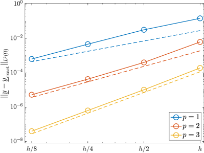
(a) No correction term.

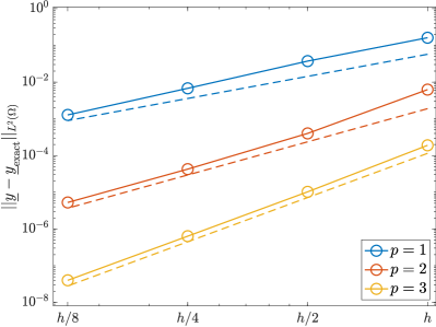
(b) Original correction term (3.8).

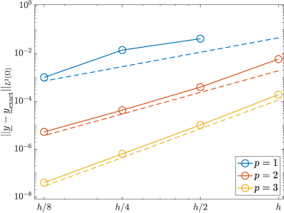
(c) Modified correction term (3.18).

Figure 4.1: Convergence under grid refinement, with $h=0.02$, for the multicomponent Gaussian-wave test. The $L^{2}$ error of the normalized state with respect to the exact solution at $t=1$ is computed. The dashed lines represent convergence rates of $p+1$.

4.2 One-dimensional, high-velocity thermal bubble

This section presents results for the high-velocity advection of a high-pressure, nitrogen/n-dodecane thermal bubble. This test case was originally presented in [52] and [12] with discontinuous initial conditions and then modified to be smooth in [3] in order to circumvent the need for discontinuity-capturing techniques. The initial condition is given by

$$v = 600\textrm{ m/s},$$

$$Y_{n\text{-}\mathrm{C_{12}H_{26}}} = \frac{1}{2}\left[1-\tanh\left(25|x|-5\right)\right],$$

$$Y_{\mathrm{N_{2}}} = 1-Y_{n\text{-}\mathrm{C_{12}H_{26}}},$$ (4.3)

$$T = \frac{T_{\min}+T_{\max}}{2}+\frac{T_{\max}-T_{\min}}{2}\tanh\left(25|x|-5\right)\textrm{ K},$$

$$P = 6\textrm{ MPa},$$

where $T_{\min}=363\text{ K}$ and $T_{\max}=900\text{ K}$. The computational domain is $\left[-0.5,0.5\right]\text{ m}$, partitioned into $25$ line cells (such that $h=0.04\;\mathrm{m}$), and $p=3$ solutions are obtained. Both sides of the domain are periodic. Note that the assumption of thermally perfect gases may not be physically accurate at these high-pressure conditions; a real-fluid model (e.g., a cubic equation of state [52, 12]) would be more appropriate. Nevertheless, this study concerns numerical accuracy, robustness, and pressure-equilibrium preservation, which we have found this case to be well-suited to assess [3].

As discussed in Remark 12, the use of explicit SSPRK schemes prevents fully discrete conservation of total energy. However, the energy-conservation error should converge at the expected rate associated with the time-integration scheme. We perform a temporal convergence study for the pressure-based schemes (P1, P2, and P3). The percent error in total-energy conservation is computed after 100 advection periods (i.e., $t=100\tau$, where $\tau$ is the time to advect the solution one period) as

$$\left|\frac{\int_{\Omega}\left.\rho e_{t}\right|_{t=100\tau}dx-\int_{\Omega}\left.\rho e_{t}\right|_{t=0}dx}{\int_{\Omega}\left.\rho e_{t}\right|_{t=0}dx}\right|\times 100.$$

Five time-step sizes are considered: $\Delta t$, $\Delta t/2$, $\Delta t/4$, $\Delta t/8$, and $\Delta t/16$, where $\Delta t=3.14\text{ $\mu s$}$. The results are given in Figure 4.2, where the dashed line represents the expected third-order convergence rate. Without the correction term (P1), the energy-conservation error does not converge with decreasing time-step size. The expected third-order convergence rate is observed with the correction terms (P2 and P3) combined with SSPRK3 time integration.

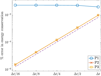
Figure 4.2: Convergence of total-energy conservation with respect to time-step size, where $\Delta t=3.14\text{ $\mu s$}$, for the one-dimensional, high-velocity thermal-bubble test case. The percent error in global energy conservation after 100 advection periods is computed. The dashed line represents a third-order rate of convergence.

Next, we assess the robustness and pressure-equilibrium errors of all considered schemes. All solutions are integrated in time until $t=100\tau$ (unless the solution diverges) with $\mathrm{CFL}=0.6$. For comparison, we also employ the total-energy-based DG scheme (2.10) with overintegration (E1) and colocated integration (E2). Figure 4.3a presents the temporal variation of the percent error in pressure. The percent error in pressure is sampled every $\tau$ seconds until the solution either diverges or is advected for 100 periods. The total-energy-based DG scheme with colocated integration diverges rapidly. With overintegration, the total-energy-based DG scheme remains stable but exhibits large errors in pressure. In contrast, the pressure-based DG scheme with the original correction term (3.8) (P2) yields significantly smaller (though not negligible) errors in pressure. The pressure deviations associated with the uncorrected pressure-based DG scheme (P1) and the proposed pressure-based DG scheme (P3) are due to finite-precision-induced errors.

Figures 4.3b and 4.3c display the pressure and temperature profiles, respectively, at $t=100\tau$ for the stable solutions. Large-scale oscillations are observed in the overintegrated total-energy-based solution. These oscillations are significantly reduced or eliminated in the pressure-based solutions, which are all visually similar.

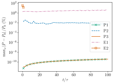
(a) Temporal variation of error in pressure.

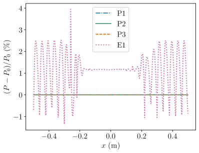
(b) Pressure profiles at $t=100\tau$.

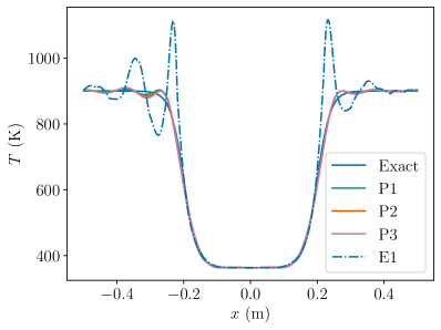
(c) Temperature profiles at $t=100\tau$.

Figure 4.3: $p=3$ solutions to the advection of a nitrogen/n-dodecane thermal bubble at $v=600\text{ m/s}$. P1: uncorrected pressure–based DG scheme; P2: pressure-based DG scheme with original correction term (3.8); P3: proposed pressure-based DG scheme (Section 3.3); E1: total-energy-based DG scheme with overintegration; E2: total-energy-based DG scheme with colocated integration; Exact: exact solution.

Next, to demonstrate the failure to preserve zero species concentrations of the original correction term, we include another species, O₂, and set $Y_{\mathrm{O_{2}}}=0$ at $t=0$. Of course, $Y_{\mathrm{O_{2}}}$ should remain zero for the entire simulation. However, as shown in Figure 4.4, there is spurious production and destruction of O₂ with the P2 scheme. This can be particularly detrimental in the case of chemically reacting flows since even trace concentrations of highly reactive species can significantly affect the solution [53, 54, 55]. With the strategy discussed in Remark 19, the proposed (P3) scheme preserves zero $Y_{\mathrm{O_{2}}}$.

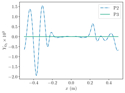
Figure 4.4: $Y_{\mathrm{O_{2}}}$ profiles at $t=100\tau$ obtained from $p=3$ solutions to the advection of a nitrogen/n-dodecane thermal bubble at $v=600\text{ m/s}$.

4.3 One-dimensional, low-velocity thermal bubble

The initial condition here is identical to that for the previous test case, except the velocity is set to $v=1\text{ m/s}$. In [3], noticeably different results (in terms of stability) were observed between the low-velocity and high-velocity case when employing a total-energy-based DG scheme with various integration strategies. The domain is partitioned into 50 cells, and $p=2$ solutions are integrated in time for ten advection periods (unless the solver crashes) with a CFL of 0.8.

Figure 4.5a presents the temporal variation of the percent error in pressure for all considered schemes, which is sampled every $\tau/10$ seconds (where $\tau$ is again the time to advect the solution one period) until the solution either diverges or is advected for ten periods. Unlike in the high-velocity case, the total-energy-based DG scheme with overintegration diverges rapidly. With colocated integration, the total-energy-based DG scheme remains stable but exhibits appreciable errors in pressure. Conversely, all pressure-based DG schemes exhibit significantly smaller errors in pressure. These errors are still present with the original correction term (3.8) and completely eliminated (apart from errors induced by finite precision) with the proposed modifications. Figures 4.5b and 4.5c display the pressure and temperature profiles, respectively, at $t=10\tau$ for the stable solutions. The colocated total-energy-based solution exhibits a nearly uniform offset from the equilibrium pressure and large-scale temperature oscillations. Significantly better agreement with the exact solution is observed for the pressure-based solutions.

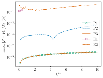
(a) Temporal variation of error in pressure.

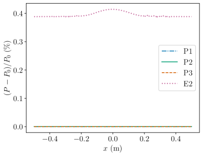
(b) Pressure profiles at $t=10\tau$.

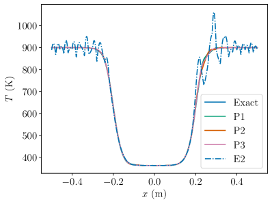
(c) Temperature profiles at $t=10\tau$.

Figure 4.5: $p=3$ solution to the advection of a nitrogen/n-dodecane thermal bubble at $v=1\text{ m/s}$. P1: uncorrected pressure–based DG scheme; P2: pressure-based DG scheme with original correction term (3.8); P3: proposed pressure-based DG scheme (Section 3.3); E1: total-energy-based DG scheme with overintegration; E2: total-energy-based DG scheme with colocated integration; Exact: exact solution.

4.4 Two-dimensional, high-velocity thermal bubble

This problem is a two-dimensional version of the high-velocity thermal-bubble test case in Section 4.2. The initial condition is given by

$$Y_{n\text{-}\mathrm{C_{12}H_{26}}} = \frac{1}{2}\left[1-\tanh\left(25\sqrt{x_{1}^{2}+x_{2}^{2}}-5\right)\right],$$

$$Y_{\mathrm{N_{2}}} = 1-Y_{n\text{-}\mathrm{C_{12}H_{26}}},$$

$$T = \frac{T_{\min}+T_{\max}}{2}+\frac{T_{\max}-T_{\min}}{2}\tanh\left(25\sqrt{x_{1}^{2}+x_{2}^{2}}-5\right)\textrm{ K},$$ (4.4)

$$P = 6\textrm{ MPa},$$

$$\left(v_{1},v_{2}\right) = \left(600,0\right)\textrm{ m/s},$$

The computational domain is $\text{$\Omega$}=\left[-0.5,0.5\right]\mathrm{m}\times\left[-0.5,0.5\right]\mathrm{m}$. The left, right, bottom, and top boundaries are periodic. Gmsh [56] is used to generate an unstructured triangular mesh with a characteristic cell size of $h=0.04\leavevmode\nobreak\ \mathrm{m}$. Figure 4.6 presents the initial $p=3$ density and temperature fields, superimposed by the mesh.

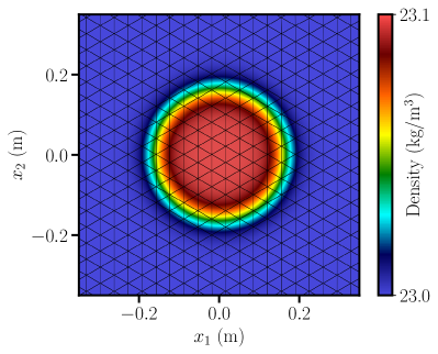
(a) Initial density field.

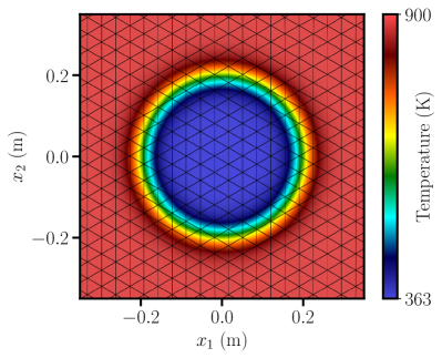
(b) Initial temperature field.

Figure 4.6: Initial $p=3$ density and pressure fields, superimposed by the grid, for the two-dimensional advection of a nitrogen/n-dodecane thermal bubble.

We first assess the temporal convergence of the pressure-based schemes in this two-dimensional setting. Four time-step sizes are considered: $\Delta t/2$, $\Delta t/4$, $\Delta t/8$, and $\Delta t/16$, where $\Delta t=3.14\text{ $\mu s$}$, as in Section 4.2. Note that, unlike in the one-dimensional version, $\Delta t$ is too large and results in solver divergence. The results are presented in Figure 4.2, where the dashed line represents the expected third-order convergence rate. The P2 solution diverges before $t=100\tau$ and is therefore not included. The expected third-order convergence rate is observed with the P3 scheme combined with SSPRK3 time integration. The P1 scheme (no correction term) results in significantly greater errors in energy conservation, which fail to converge with decreasing time-step size.

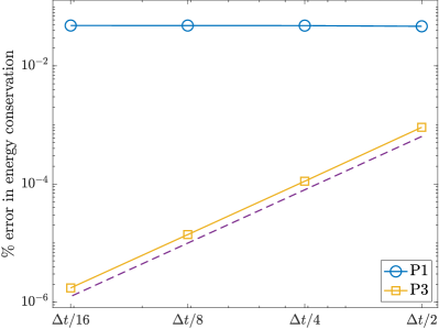
Figure 4.7: Convergence of total-energy conservation with respect to time-step size, where $\Delta t=3.14\text{ $\mu s$}$, for the two-dimensional, high-velocity thermal-bubble test case. The percent error in global energy conservation after 100 advection periods is computed. The dashed line represents a third-order rate of convergence.

Figure 4.8 presents the temporal variation of percent error in pressure, sampled every $\tau$ seconds, for all considered schemes. Specifically, $p=3$ solutions are integrated in time with a CFL of 0.6 until either $t=100\tau$ or the solution diverges. The total-energy-based DG scheme with colocated integration diverges rapidly. Unlike in the one-dimensional setting, the total-energy-based DG scheme with colocated integration and the pressure-based DG scheme with the original correction term (3.8) diverge before $t=100\tau$. The small pressure deviations observed for the uncorrected pressure-based DG scheme and the proposed scheme are due to finite-precision issues.

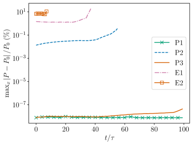
Figure 4.8: Temporal variation of error in pressure for $p=3$ solutions to the two-dimensional advection of a nitrogen/n-dodecane thermal bubble. P1: uncorrected pressure–based DG scheme; P2: pressure-based DG scheme with original correction term (3.8); P3: proposed pressure-based DG scheme (Section 3.3); E1: total-energy-based DG scheme with overintegration; E2: total-energy-based DG scheme with colocated integration; Exact: exact solution.

Figures 4.9 and 4.10 display the final density and temperature fields for the P1 and P3 schemes, respectively. The shape of the bubble is well-maintained in both cases due to the absence of any pressure and velocity disturbances.

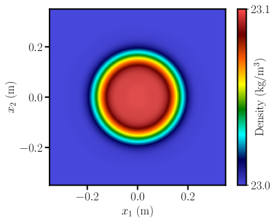
(a) Density.

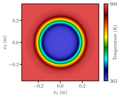
(b) Temperature.

Figure 4.9: $p=3$ solution to two-dimensional advection of a nitrogen/n-dodecane thermal bubble at $t=100\tau$ computed with the uncorrected DG scheme (P1).

(a) Density.

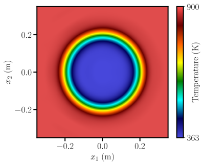
(b) Temperature.

Figure 4.10: $p=3$ solution to two-dimensional advection of a nitrogen/n-dodecane thermal bubble at $t=100\tau$ computed with the proposed pressure-based DG scheme (P3).

Curved elements

Finally, we recompute this case using curved elements of quadratic order with a CFL of 0.4. To generate the curved mesh, high-order geometric nodes are inserted at the midpoints of the vertices of each element. At interior edges, the midpoint nodes are randomly perturbed by a distance up to $0.05h$. Figure 4.11 presents the temporal variation of percent error in pressure for all considered schemes. Again, only the P1 and P3 schemes remain stable for 100 advection periods. Interestingly, the E2 scheme maintains stability for longer times, and the P2 (original correction formulation) solution diverges earlier than the E1 solution.

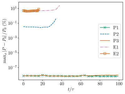
Figure 4.11: Temporal variation of error in pressure for $p=3$ solutions to the two-dimensional advection of a nitrogen/n-dodecane thermal bubble on a curved grid. P1: uncorrected pressure–based DG scheme; P2: pressure-based DG scheme with original correction term (3.8); P3: proposed pressure-based DG scheme (Section 3.3); E1: total-energy-based DG scheme with overintegration; E2: total-energy-based DG scheme with colocated integration; Exact: exact solution.

Figures 4.12 and 4.13 display the final density and temperature fields for the P1 and P3 schemes, respectively, superimposed by the curved grid. Just as with the straight-sided grid, the shape of the bubble is well-maintained in both cases due to the absence of any pressure and velocity disturbances.

(a) Density.

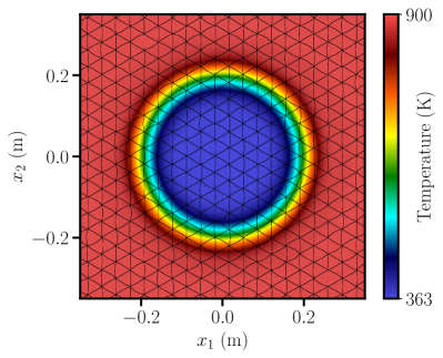
(b) Temperature.

Figure 4.12: $p=3$ solution to two-dimensional advection of a nitrogen/n-dodecane thermal bubble at $t=100\tau$ computed with the uncorrected DG scheme (P1) on a curved grid.

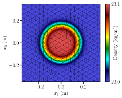
(a) Density.

(b) Temperature.

Figure 4.13: $p=3$ solution to two-dimensional advection of a nitrogen/n-dodecane thermal bubble at $t=100\tau$ computed with the proposed pressure-based DG scheme (P3) on a curved grid.

4.5 Three-dimensional, high-velocity thermal bubble

Our final test case is a three-dimensional version of the high-velocity thermal-bubble problem in Section 4.2. The initial condition is given by

$$Y_{n\text{-}\mathrm{C_{12}H_{26}}} = \frac{1}{2}\left[1-\tanh\left(25\sqrt{x_{1}^{2}+x_{2}^{2}+x_{3}^{2}}-5\right)\right],$$

$$Y_{\mathrm{N_{2}}} = 1-Y_{n\text{-}\mathrm{C_{12}H_{26}}},$$

$$T = \frac{T_{\min}+T_{\max}}{2}+\frac{T_{\max}-T_{\min}}{2}\tanh\left(25\sqrt{x_{1}^{2}+x_{2}^{2}+x_{3}^{2}}-5\right)\textrm{ K},$$ (4.5)

$$P = 6\textrm{ MPa},$$

$$\left(v_{1},v_{2},v_{3}\right) = \left(600,0,0\right)\textrm{ m/s},$$

The computational domain is $\text{$\Omega$}=\left[-0.5,0.5\right]\mathrm{m}\times\left[-0.5,0.5\right]\mathrm{m}\times\left[-0.5,0.5\right]\mathrm{m}$. All boundaries are periodic. Gmsh [56] is used to generate an unstructured triangular mesh with a characteristic cell size of $h=0.02\leavevmode\nobreak\ \mathrm{m}$. Figure 4.14 presents $T=890\;\mathrm{K}$ isosurfaces colored by density at $t=0$.

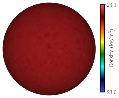
Figure 4.14: $T=890\;\mathrm{K}$ isosurfaces colored by density at $t=0$ for the three-dimensional advection of a nitrogen/n-dodecane thermal bubble.

Figure 4.15 presents the temporal variation of percent error in pressure, sampled every $\tau$ seconds, for all considered schemes. $p=3$ solutions are integrated in time with a CFL of 0.6 until either $t=100\tau$ or the solution diverges. As in the two-dimensional setting, only the pressure-based DG schemes without any correction (P1) and with the proposed correction formulation (P3) remain stable through $t=100\tau$. The total-energy-based scheme with colocated integration (E2) diverges the earliest, followed by the pressure-based DG scheme with the original correction term (P2). The small pressure deviations observed for the P1 and P3 schemes are due to finite-precision issues.

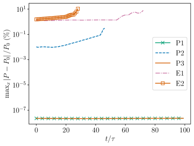
Figure 4.15: Temporal variation of error in pressure for $p=3$ solutions to the three-dimensional advection of a nitrogen/n-dodecane thermal bubble. P1: uncorrected pressure–based DG scheme; P2: pressure-based DG scheme with original correction term (3.8); P3: proposed pressure-based DG scheme (Section 3.3); E1: total-energy-based DG scheme with overintegration; E2: total-energy-based DG scheme with colocated integration; Exact: exact solution.

Figure 4.16 the temperature isosurfaces (colored by density) at $t=100\tau$ computed with the P1 and P3 schemes, respectively. Although density variations are observed, they remain marginal, and the shape of the bubble is well-maintained in both cases.

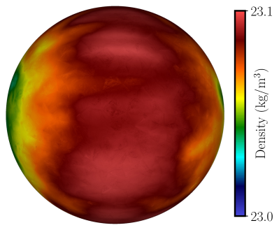
(a) Uncorrected scheme (P1).

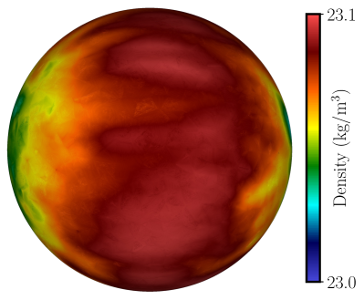
(b) Proposed scheme (P3).

Figure 4.16: $T=890\;\mathrm{K}$ isosurfaces colored by density at $t=100\tau$ for the three-dimensional advection of a nitrogen/n-dodecane thermal bubble computed with the P1 and P3 schemes.

5 Concluding remarks

In this work, we analyzed the velocity-equilibrium and pressure-equilibrium conditions of a standard DG scheme that discretizes the conservative form of the compressible, multicomponent Euler quations. It was shown that under certain constraints on the numerical flux, the scheme is velocity-equilibrium-preserving. However, standard DG schemes are not pressure-equilibrium-preserving. Therefore, a pressure-based formulation was adopted (i.e., the total-energy conservation equation is replaced by pressure-evolution equation). In order to restore the (semi-discrete) total-energy conservation that is otherwise lost, we incorporated the conservative, elementwise correction terms of Abgrall [1] and Abgrall et al. [2]. Unfortunately, the corrected pressure-based DG scheme no longer exactly preserves pressure and velocity equilibria. Furthermore, it does not preserve zero species concentrations. To address these issues, we proposed simple modifications to the correction term that then enable preservation of pressure equilibrium, velocity equilibrium, and zero species concentrations, in addition to semidiscrete conservation of total energy. Since the elementwise correction terms are not valid if the state inside a given element is uniform, we also introduced face-based corrections, inspired by [30], along with a particular definition of the numerical total-energy flux, to account for the case of elementwise-constant solutions with inter-element jumps. We applied the scheme to compute smooth, interfacial flows initially in velocity and pressure equilibria. In the first test case, optimal convergence was demonstrated. However, the proposed modifications may introduce additional errors that primarily manifest in $p=1$ solutions (although $p\geq 2$ solutions seem largely unaffected). The next two test cases entailed high-velocity and low-velocity advection of a nitrogen/n-dodecane thermal bubble in one dimension. A total-energy-based DG formulation with colocated integration failed to maintain solution stability in the former, while a total-energy-based formulation with overintegration failed to maintain stability in the latter. The pressure oscillations were significantly reduced, but not eliminated, using the pressure-based DG scheme with the original correction term. With the proposed modifications, both pressure-equilibrium preservation and semidiscrete conservation of total energy were achieved. In two- and three-dimensional versions of the high-velocity nitrogen/n-dodecane thermal-bubble problem, the pressure-based DG scheme with the original correction term resulted in solver divergence, while the developed scheme maintained solution stability due to exact preservation of pressure equilibrium (apart from minor finite-precision-induced errors).

Note that apart from pressure-equilibrium preservation, there are certain advantages to using a pressure-based formulation instead of a total-energy-based formulation. For example, in the former, temperature is straightforward to compute from the state; in contrast, an iterative solver is typically required to obtain temperature from the state in the latter. In addition, the occurrence of negative pressures is a major issue in underresolved smooth regions and near discontinuities that can lead to solver divergence; it is possible that negative pressures are more likely to happen in a total-energy-based formulation since pressure is a nonlinear function of the state, although this requires further investigation. In certain cases, it may be easier to guarantee positive pressures in a pressure-based formulation since pressure is a state variable (though this is outside the scope of the current study). At the same time, there are disadvantages to using a pressure-based formulation as well. For instance, in the case of viscous flows, the discretization of the additional terms may not be straightforward. Furthermore, limiters that are conservative in total-energy-based formulations do not necessarily conserve total energy in pressure-based formulations. Entropy-based stabilization techniques that rely on a total-energy-based formulation may also be difficult to apply.

There are many potential directions for future work. The current scheme is designed for smooth flows initially in velocity and pressure equilibria; we plan to extend it to flows with discontinuities by incorporating appropriate stabilization mechanisms. The modified correction term may not be appropriate in the case of non-uniform velocity and pressure, in which case the original correction term is more suitable; therefore, we may adopt a hybrid strategy that switches between the two correction terms in such a way that guarantees semidiscrete conservation of total energy and, where appropriate, preservation of pressure and velocity equilibrium. Another hybrid approach is to switch to a total-energy formulation when pressure-equilibrium preservation is not applicable, although this may introduce new complications; note that such an approach would be distinct from other hybrid schemes in the literature that combine total-energy-based and pressure-based formulations due to semidiscrete satisfaction of total-energy conservation in the entire domain. To handle discontinuities, we will explore stabilization techniques that do not cause loss of these properties. Furthermore, we will conduct a detailed investigation of the importance of conserving total energy in regions away from shocks, particularly in large-scale, practical flow problems. An additional matter we aim to address is the importance of fully discrete (as opposed to semidiscrete) conservation of total energy, which would require the use of specific time integrators. Finally, we will consider viscous effects, chemical reactions, and real-fluid mixtures, which are much more susceptible to spurious pressure oscillations and other nonlinear instabilities, and perform in-depth comparisons with state-of-the-art total-energy-based formulations.

Appendix A Compressible vortex transport: Grid convergence

In this section, we study convergence under grid refinement of the DG discretization (3.4) in order to test our implementation of the nonconservative terms, especially since the cases in Section 4 involve flows initially in pressure and velocity equilibria, such that the nonconservative terms vanish (assuming pressure equilibrium is discretely preserved). We consider vortex advection based on the configuration presented in [39]. The initial condition is written in nondimensional form as

$$v_{1} = v_{\infty}-\frac{\sigma}{2\pi}\left(x_{2}-x_{c,2}\right)\exp\left(1-r^{2}\right),$$

$$v_{2} = v_{\infty}+\frac{\sigma}{2\pi}\left(x_{1}-x_{c,1}\right)\exp\left(1-r^{2}\right),$$

$$\rho = \left[1-\frac{\sigma^{2}\left(\gamma-1\right)}{16\pi^{2}\gamma}\exp\left(2-2r^{2}\right)\right]^{\frac{1}{\gamma-1}},$$

$$P = \rho^{\gamma},$$

where $v_{\infty}=10$, $r=\sqrt{\left(x_{1}-x_{c,1}\right)^{2}+\left(x_{2}-x_{c,2}\right)^{2}}$, $\sigma=4$ is the vortex strength, and $\gamma=1.4$. The computational domain is $\text{$\Omega$}=\left[0,L\right]^{2}$, where $L=10$, and the vortex center is $\left(x_{c,1},x_{c,2}\right)=\left(L/2,L/2\right).$ All boundaries are periodic, and all simulations are run for one advection period with a CFL of 0.1, as defined in Equation (4.14). Figure A.1 presents the $L^{2}$ errors of the state variables (normalized as discussed in Section 4.1) for $p=1$ to $p=3$ and four grid sizes, where the coarsest grid size is $h=1$. The dashed lines represent convergence rates of $p+1$. Optimal convergence is observed.

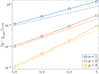
Figure A.1: Convergence under grid refinement, with $h=1$, for the vortex-transport problem. The $L^{2}$ error of the normalized state with respect to the exact solution after one advection period is computed. The dashed lines represent convergence rates of $p+1$.

Appendix B Derivative of total energy with respect to the state

This section provides a derivation of $\bm{w}=\partial_{\bm{y}}\left(\rho e_{t}\right)$ in Equation (3.10). The perturbation of total energy, $\rho e_{t}=\rho u+\frac{1}{2}\rho\sum_{k=1}^{d}v_{k}v_{k}$, is given by

$$\delta\rho e_{t}=\left(\frac{\partial\rho u}{\partial T}\right)_{C_{i}}\delta T+\sum_{i=1}^{n_{s}}\left(\frac{\partial\rho u}{\partial C_{i}}\right)_{T,C_{j\neq i}}\delta C_{i}+\sum_{k=1}^{d}v_{k}\delta\left(\rho v_{k}\right)-\frac{1}{2}\sum_{k=1}^{d}v_{k}v_{k}\delta\rho.$$ (B.1)

With $T=T\left(C_{1},\ldots,C_{n_{s}},P\right)$, the temperature perturbation can be written as

$$\delta T=\left(\frac{\partial T}{\partial P}\right)_{C_{i}}\delta P+\sum_{i=1}^{n_{s}}\left(\frac{\partial T}{\partial C_{i}}\right)_{P,C_{i\neq i}}\delta C_{i}$$ (B.2)

Substituting Equation (B.2) into Equation (B.1) yields

$$\delta\rho e_{t}= \left(\frac{\partial\rho u}{\partial T}\right)_{C_{i}}\left(\frac{\partial T}{\partial P}\right)_{C_{i}}\delta P+\left(\frac{\partial\rho u}{\partial T}\right)_{C_{i}}\sum_{i=1}^{n_{s}}\left(\frac{\partial T}{\partial C_{i}}\right)_{P,C_{i\neq i}}\delta C_{i}+\sum_{i=1}^{n_{s}}\left(\frac{\partial\rho u}{\partial C_{i}}\right)_{T,C_{j\neq i}}\delta C_{i}$$

$$+\sum_{k=1}^{d}v_{k}\delta\left(\rho v_{k}\right)-\frac{1}{2}\sum_{k=1}^{d}v_{k}v_{k}\sum_{i=1}^{n_{s}}W_{i}\delta C_{i}$$

$$= \sum_{k=1}^{d}v_{k}\delta\left(\rho v_{k}\right)+\left(\frac{\partial\rho u}{\partial T}\right)_{C_{i}}\left(\frac{\partial T}{\partial P}\right)_{C_{i}}\delta P+\sum_{i=1}^{n_{s}}\left[\left(\frac{\partial\rho u}{\partial T}\right)_{C_{i}}\left(\frac{\partial T}{\partial C_{i}}\right)_{P,C_{i\neq i}}+\left(\frac{\partial\rho u}{\partial C_{i}}\right)_{T,C_{j\neq i}}-\frac{W_{i}}{2}\sum_{k=1}^{d}v_{k}v_{k}\right]\delta C_{i},$$

which gives

$$\bm{w} =\frac{\partial\left(\rho e_{t}\right)}{\partial\bm{y}}$$

$$=\left(\begin{array}[]{ccc}\frac{\partial\left(\rho e_{t}\right)}{\partial\rho v_{k}},&\frac{\partial\left(\rho e_{t}\right)}{\partial P},&\frac{\partial\left(\rho e_{t}\right)}{\partial C_{i}}\end{array}\right)^{T}$$

$$=\left(\begin{array}[]{ccc}v_{k},&\left(\frac{\partial\rho u}{\partial T}\right)_{C_{i}}\left(\frac{\partial T}{\partial P}\right)_{C_{i}},&\left(\frac{\partial\rho u}{\partial T}\right)_{C_{i}}\left(\frac{\partial T}{\partial C_{i}}\right)_{P,C_{i\neq i}}+\left(\frac{\partial\rho u}{\partial C_{i}}\right)_{T,C_{j\neq i}}-\frac{W_{i}}{2}\sum_{k=1}^{d}v_{k}v_{k}\end{array}\right)^{T}.$$

The equation of state (2.5) results in

$$\left(\frac{\partial T}{\partial P}\right)_{C_{i}}=\frac{1}{R^{0}\sum_{i}C_{i}},\quad\left(\frac{\partial T}{\partial C_{i}}\right)_{P,C_{j\neq i}}=-\frac{P}{R^{0}\left(\sum_{i}C_{i}\right)^{2}}.$$

Introducing the mass-specific heat capacity at constant volume of the $i$th species, $c_{v,i}=c_{p,i}-R_{i}$, and $\rho c_{v}=\sum_{i=1}^{n_{s}}\rho_{i}c_{v,i}$, we have

$$\left(\frac{\partial\rho u}{\partial T}\right)_{C_{i}}=\rho c_{v},\quad\left(\frac{\partial\rho u}{\partial C_{i}}\right)_{T,C_{j\neq i}}=W_{i}u_{i}.$$

$\bm{w}$ can then be expressed as

$$\bm{w}=\left(\begin{array}[]{ccc}v_{k},&\frac{\rho c_{v}}{R^{0}\sum_{j}C_{j}},&W_{i}u_{i}-\frac{\rho c_{v}P}{R^{0}\left(\sum_{j}C_{j}\right)^{2}}-\frac{W_{i}}{2}\bm{v}\cdot\bm{v}\end{array}\right)^{T}.$$

References

- [1] R. Abgrall, A general framework to construct schemes satisfying additional conservation relations. application to entropy conservative and entropy dissipative schemes, Journal of Computational Physics 372 (2018) 640–666.
- [2] R. Abgrall, P. Öffner, H. Ranocha, Reinterpretation and extension of entropy correction terms for residual distribution and discontinuous Galerkin schemes: application to structure preserving discretization, Journal of Computational Physics 453 (2022) 110955.
- [3] E. J. Ching, R. F. Johnson, A. D. Kercher, A note on reducing spurious pressure oscillations in fully conservative discontinuous Galerkin simulations of multicomponent flows, arXiv preprint arXiv:2310.17792 (2023).
- [4] R. Abgrall, S. Karni, Computations of compressible multifluids, Journal of Computational Physics 169 (2) (2001) 594 – 623. doi:https://doi.org/10.1006/jcph.2000.6685.
- [5] S. Karni, Viscous shock profiles and primitive formulations, SIAM journal on numerical analysis 29 (6) (1992) 1592–1609.
- [6] S. Karni, Multicomponent flow calculations by a consistent primitive algorithm, Journal of Computational Physics 112 (1) (1994) 31 – 43. doi:https://doi.org/10.1006/jcph.1994.1080.
- [7] H. Terashima, M. Koshi, Approach for simulating gas liquid-like flows under supercritical pressures using a high-order central differencing scheme, Journal of Computational Physics 231 (20) (2012) 6907 – 6923. doi:https://doi.org/10.1016/j.jcp.2012.06.021.
- [8] S. Kawai, H. Terashima, H. Negishi, A robust and accurate numerical method for transcritical turbulent flows at supercritical pressure with an arbitrary equation of state, Journal of Computational Physics 300 (2015) 116–135.
- [9] S. Karni, Hybrid multifluid algorithms, SIAM Journal on Scientific Computing 17 (5) (1996) 1019–1039.
- [10] R. Fedkiw, X.-D. Liu, S. Osher, A general technique for eliminating spurious oscillations in conservative schemes for multiphase and multispecies Euler equations, International Journal of Nonlinear Sciences and Numerical Simulation 3 (2) (2002) 99–106.
- [11] Y. Lv, M. Ihme, Discontinuous Galerkin method for multicomponent chemically reacting flows and combustion, Journal of Computational Physics 270 (2014) 105 – 137. doi:https://doi.org/10.1016/j.jcp.2014.03.029.
- [12] B. Boyd, D. Jarrahbashi, A diffuse-interface method for reducing spurious pressure oscillations in multicomponent transcritical flow simulations, Computers & Fluids 222 (2021) 104924.
- [13] E. Gaburro, W. Boscheri, S. Chiocchetti, M. Ricchiuto, Discontinuous Galerkin schemes for hyperbolic systems in non-conservative variables: quasi-conservative formulation with subcell finite volume corrections, Computer Methods in Applied Mechanics and Engineering 431 (2024) 117311.
- [14] W. H. Reed, T. Hill, Triangular mesh methods for the neutron transport equation, Tech. rep., Los Alamos Scientific Lab., N. Mex.(USA) (1973).
- [15] F. Bassi, S. Rebay, High-order accurate discontinuous finite element solution of the 2D Euler equations, Journal of Computational Physics 138 (2) (1997) 251–285.
- [16] F. Bassi, S. Rebay, A high-order accurate discontinuous finite element method for the numerical solution of the compressible Navier–Stokes equations, Journal of Computational Physics 131 (2) (1997) 267–279.
- [17] B. Cockburn, C.-W. Shu, The Runge–Kutta discontinuous Galerkin method for conservation laws V: multidimensional systems, Journal of Computational Physics 141 (2) (1998) 199–224.
- [18] B. Cockburn, G. Karniadakis, C.-W. Shu, The development of discontinuous Galerkin methods, in: Discontinuous Galerkin Methods, Springer, 2000, pp. 3–50.
- [19] Z. Wang, K. Fidkowski, R. Abgrall, F. Bassi, D. Caraeni, A. Cary, H. Deconinck, R. Hartmann, K. Hillewaert, H. Huynh, N. Kroll, G. May, P.-O. Persson, B. van Leer, M. Visbal, High-order CFD methods: Current status and perspective, International Journal for Numerical Methods in Fluids (2013). doi:10.1002/fld.3767.
- [20] R. F. Johnson, A. D. Kercher, A conservative discontinuous Galerkin discretization for the chemically reacting Navier–Stokes equations, Journal of Computational Physics 423 (2020) 109826. doi:10.1016/j.jcp.2020.109826.
- [21] K. Bando, Towards high-performance discontinuous Galerkin simulations of reacting flows using Legion, Ph.D. thesis, Stanford University (2023).
- [22] T. Johnsen, T. Colonius, Implementation of WENO schemes in compressible multicomponent flow problems, Journal of Computational Physics 219 (2) (2006) 715 – 732. doi:https://doi.org/10.1016/j.jcp.2006.04.018.
- [23] N. Franchina, M. Savini, F. Bassi, Multicomponent gas flow computations by a discontinuous Galerkin scheme using L2-projection of perfect gas EOS, Journal of Computational Physics 315 (2016) 302–322.
- [24] Y. Fujiwara, Y. Tamaki, S. Kawai, Fully conservative and pressure-equilibrium preserving scheme for compressible multi-component flows, Journal of Computational Physics 478 (2023) 111973.
- [25] H. Terashima, N. Ly, M. Ihme, Approximately pressure-equilibrium-preserving scheme for fully conservative simulations of compressible multi-species and real-fluid interfacial flows, Journal of Computational Physics 524 (2025) 113701.
- [26] T. Chen, C.-W. Shu, Review of entropy stable discontinuous Galerkin methods for systems of conservation laws on unstructured simplex meshes, CSIAM Transactions on Applied Mathematics 1 (1) (2020) 1–52.
- [27] E. Gaburro, P. Öffner, M. Ricchiuto, D. Torlo, High order entropy preserving ADER-DG schemes, Applied Mathematics and Computation 440 (2023) 127644.
- [28] Y. Mantri, P. Öffner, M. Ricchiuto, Fully well-balanced entropy controlled discontinuous Galerkin spectral element method for shallow water flows: Global flux quadrature and cell entropy correction, Journal of Computational Physics 498 (2024) 112673.
- [29] L. Alberti, E. Carnevali, A. Colombo, A. Crivellini, An entropy conserving/stable discontinuous Galerkin solver in entropy variables based on the direct enforcement of entropy balance, Journal of Computational Physics 508 (2024) 113007.
- [30] R. Abgrall, S. Busto, M. Dumbser, A simple and general framework for the construction of thermodynamically compatible schemes for computational fluid and solid mechanics, Applied Mathematics and Computation 440 (2023) 127629.
- [31] M. J. Castro, P. G. LeFloch, M. L. Muñoz-Ruiz, C. Parés, Why many theories of shock waves are necessary: Convergence error in formally path-consistent schemes, Journal of Computational Physics 227 (17) (2008) 8107–8129.
- [32] R. Abgrall, S. Karni, A comment on the computation of non-conservative products, Journal of Computational Physics 229 (8) (2010) 2759–2763.
- [33] V. Giovangigli, Multicomponent flow modeling, Birkhauser, Boston, 1999.
- [34] B. J. McBride, S. Gordon, M. A. Reno, Coefficients for calculating thermodynamic and transport properties of individual species (1993).
- [35] B. J. McBride, M. J. Zehe, S. Gordon, NASA Glenn coefficients for calculating thermodynamic properties of individual species (2002).
- [36] E. J. Ching, R. F. Johnson, S. Burrows, J. Higgs, A. D. Kercher, Positivity-preserving and entropy-bounded discontinuous Galerkin method for the chemically reacting, compressible Navier-Stokes equations, arXiv preprint arXiv:2310.17637 (2023).
- [37] E. Toro, Riemann solvers and numerical methods for fluid dynamics: A practical introduction, Springer Science & Business Media, 2013.
- [38] S. Gottlieb, C. Shu, E. Tadmor, Strong stability-preserving high-order time discretization methods, SIAM review 43 (1) (2001) 89–112.
- [39] Y. Lv, Development of a nonconservative discontinuous Galerkin formulation for simulations of unsteady and turbulent flows, International Journal for Numerical Methods in Fluids 92 (5) (2020) 325–346.
- [40] J. Chan, On discretely entropy conservative and entropy stable discontinuous Galerkin methods, Journal of Computational Physics 362 (2018) 346–374.
- [41] H. Atkins, C. Shu, Quadrature-free implementation of discontinuous Galerkin methods for hyperbolic equations, ICASE Report 96-51, 1996, Tech. rep., NASA Langley Research Center, nASA-CR-201594 (August 1996).
- [42] H. L. Atkins, C.-W. Shu, Quadrature-free implementation of discontinuous Galerkin method for hyperbolic equations, AIAA Journal 36 (5) (1998) 775–782.
- [43] J. Nordström, T. Lundquist, Summation-by-parts in time, Journal of Computational Physics 251 (2013) 487–499.
- [44] H. Ranocha, M. Sayyari, L. Dalcin, M. Parsani, D. I. Ketcheson, Relaxation Runge–Kutta methods: Fully discrete explicit entropy-stable schemes for the compressible Euler and Navier–Stokes equations, SIAM Journal on Scientific Computing 42 (2) (2020) A612–A638.
- [45] H. Ranocha, L. Lóczi, D. I. Ketcheson, General relaxation methods for initial-value problems with application to multistep schemes, Numerische Mathematik 146 (4) (2020) 875–906.
- [46] C. Wang, X. Zhang, C.-W. Shu, J. Ning, Robust high order discontinuous Galerkin schemes for two-dimensional gaseous detonations, Journal of Computational Physics 231 (2) (2012) 653–665.
- [47] X. Zhang, C.-W. Shu, On positivity-preserving high order discontinuous Galerkin schemes for compressible Euler equations on rectangular meshes, Journal of Computational Physics 229 (23) (2010) 8918–8934.
- [48] E. J. Ching, R. F. Johnson, A. D. Kercher, Positivity-preserving and entropy-bounded discontinuous Galerkin method for the chemically reacting, compressible Euler equations. Part I: The one-dimensional case, Journal of Computational Physics (2024) 112881.
- [49] R. F. Johnson, A. D. Kercher, The nondimensionalization of the chemically reacting Navier-Stokes equations, Tech. Rep. NRL/6041/MR–2022/4, U.S. Naval Research Laboratory (2022).
- [50] R. F. Johnson, A. D. Kercher, A conservative discontinuous Galerkin discretization for the chemically reacting Navier–Stokes equations, Journal of Computational Physics 423 (2020) 109826. doi:10.1016/j.jcp.2020.109826.
- [51] W. Trojak, T. Dzanic, Positivity-preserving discontinuous spectral element methods for compressible multi-species flows, Computers & Fluids 280 (2024) 106343.
- [52] P. C. Ma, Y. Lv, M. Ihme, An entropy-stable hybrid scheme for simulations of transcritical real-fluid flows, Journal of Computational Physics 340 (2017) 330–357.
- [53] A. E. Magzumov, I. A. Kirillov, V. D. Rusanov, Effect of small additives of ozone and hydrogen peroxide on the induction-zone length of hydrogen-air mixtures in a one-dimensional model of a detonation wave, Combustion, Explosion and Shock Waves 34 (1998) 338–341.
- [54] J. Crane, X. Shi, A. V. Singh, Y. Tao, H. Wang, Isolating the effect of induction length on detonation structure: Hydrogen–oxygen detonation promoted by ozone, Combustion and Flame 200 (2019) 44–52.
- [55] E. J. Ching, R. F. Johnson, Effect of ozone sensitization on the reflection patterns and stabilization of standing detonation waves induced by curved ramps, arXiv preprint arXiv:2410.13845 https://arxiv.org/abs/2410.13845 (2024).
- [56] C. Geuzaine, J.-F. Remacle, Gmsh: A three-dimensional finite element mesh generator with built-in pre- and post-processing facilities, International Journal for Numerical Methods in Engineering (79(11)) (2009) 1310–1331.