Analyzer-less X-ray Interferometry with Super-Resolution Methods

Abstract

We propose the use of super-resolution methods for X-ray grating interferometry without an analyzer with detectors that fail to meet the Nyquist sampling rate needed for traditional image recovery algorithms. This method enables Talbot-Lau interferometry without the X-ray absorbing analyzer and allows for higher autocorrelation lengths for the analyzer-less Modulated Phase Grating Interferometer. This will allow for reduced X-ray dose and higher autocorrelation lengths than previously accessible. We demonstrate the use of super-resolution methods to iteratively reconstruct attenuation, differential-phase, and dark-field images using simulations of a one-dimensional lung phantom with tumors. For a fringe period of $p_{D}=22\>\mu m$, we compare the simulated imaging performance of interferometers with a 30 $\mu m$ and 50 $\mu m$ detector for various signal-to-noise ratios. We show that our super-resolution iterative reconstruction methods are highly robust and can be used to improve grating interferometry for cases where traditional algorithms cannot be used.

1. Introduction

X-ray grating interferometry is a phase-sensitive imaging technique that simultaneously captures attenuation, differential-phase, and dark-field images. The attenuation image shows X-ray absorption, similar to a traditional radiograph, while the differential-phase and dark-field images show X-ray refraction and small angle scatter. With the introduction of differential-phase and dark-field images, X-ray interferometry has a wide variety of potential applications, including lung imaging [1, 2, 3, 4], breast imaging [5, 6, 7, 8], arthritis imaging [9, 10], osteoporosis imaging [11], additive manufacturing quality assurance [12, 13] and porosimetry [14].

The traditional Talbot-Lau Interferometer (TLI) [15, 16, 17, 18], as shown in Figure 1(a), uses a binary phase grating (labeled G1) to produce a high-resolution fringe pattern that cannot be resolved by traditional X-ray detectors. A second grating (labeled G2) serves as an analyzer grating to resolve the sub-pixel fringe patterns. The Modulated Phase Grating Interferometer (MPGI), as shown in Figure 1(b), uses a single modulated phase grating to produce directly resolvable fringe patterns [19, 20, 21, 22, 23]. The MPG has bar heights that follow an envelope function with a relatively large period, $W$. The envelope function is sampled at a high frequency pitch, $p$, to maintain the same coherence requirements as that of the TLI. The autocorrelation length is given by $ACL=\lambda D_{OD}/p_{D}$, where $\lambda$ is the peak wavelength, $D_{OD}$ is the object-to-detector distance, and $p_{D}$ is the fringe period. The ACL is important for dark-field imaging of objects with higher porosity, since the ACL determines the amount of dark-field signal produced by different scattering structures [24, 23, 25].

The TLI is the most prevalent interferometer and is at the forefront of preclinical and clinical studies [1, 2, 3, 4, 5, 6, 7, 8, 9, 10]. However, since the analyzer is an absorption grating, half of the X-rays are lost, increasing the dose by at least a factor of 2. While the MPGI does not require an analyzer grating, resolving the interference fringes directly means that the fringe period at the detector, $p_{D}$, must be at least twice the detector pixel size to meet the Nyquist criterion. Since the ACL is inversely proportional to the fringe period, this leads to lower autocorrelation lengths (ACL) for some cases.

In this work, we employ super-resolution methods [26] for the TLI and MPGI. Super-resolution allows for the removal of the analyzer grating in the TLI to reduce X-ray dose and allow for a decrease in the envelope period of the MPG to increase the ACL. We use iterative reconstruction to recover the attenuation, differential-phase, and dark-field images. In addition to reducing the X-ray dose for the TLI and allowing for higher ACL for the MPGI, the use of iterative reconstruction has the potential to improve resolution and reduce noise in the reconstructed images. For the TLI, the elimination of the analyzer grating will have the added benefits of reduced cost and easier setup.

Super-resolution methods have been used by scientists/engineers for decades for various applications [26, 27, 28], including angular super-resolution with standard X-ray systems to measure small angle X-ray scattering (SAXS) data [28]. This involved measurement of the angular distribution of SAXS, without the spatial localization information afforded by interferometric dark-field imaging. Our method is novel in that it applies super-resolution techniques (using phase-steps to increase sampling rate and then deblur and estimate using iterative reconstruction) for interferometry for the primary purpose of resolving fringes without the analyzer. To the best of our knowledge no one has attempted this before. Improvement of resolution also comes automatically with the method. The effective resolution can be as high as the phase-step resolution (sub-detector pixel) instead of the pixel size.

Previous methods exist for iterative 3D reconstruction of attenuation and differential-phase images, employing significantly different approaches [29, 30, 31, 32, 33]. They do not incorporate dark-field (SAXS) recovery. The key focus of this work is on applying iterative reconstruction to initially recover the projection images of the three modalities themselves, particularly when acquired with under-sampled conditions. For cases with multiple projection angles for tomographic interferometry, additional processing using standard analytical or iterative 3D reconstruction techniques can be used.

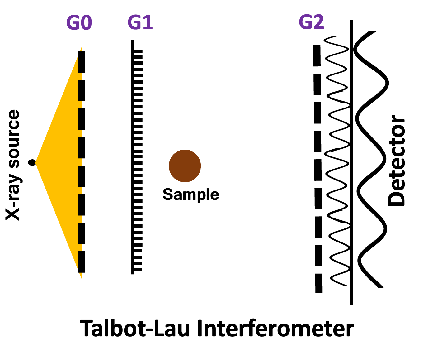
(a)

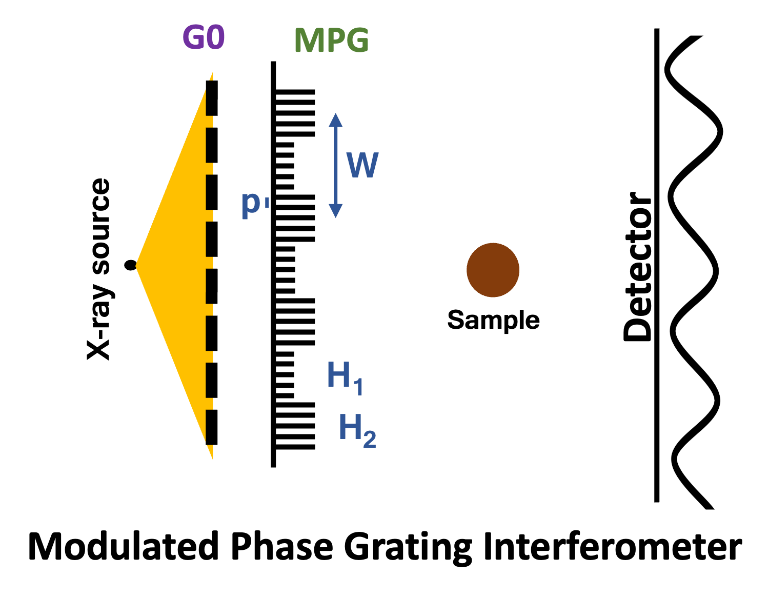
(b)

Figure 1: Schematics of the (a) Talbot-Lau and (b) Modulated Phase Grating Interferometers.

2. Methods

2.1. Image Simulation

One-dimensional interferometry signals are simulated at sub-pixel phase steps by calculating the interference fringes with and without the object in place, referred to as the ‘reference’ and ‘object’ signals. The simulations are system agnostic, and the signals are approximated as perfect sinusoids. The source and detector blur are then applied, detector sub-sampling is simulated, and Poisson noise is added. The reference image for each phase step is calculated using Equation 1, where $A$ is the amplitude of the fringe pattern, $B$ is the bias, $t_{k}$ is the translation of the k-th phase step, and $p_{D}$ is the fringe period at the detector. The fringe visibility is represented as $A/B$.

$$g^{k}_{r}(x)=A\cos\left[\frac{2\pi}{p_{D}}\left(x+t_{k}\right)\right]+B$$ (1)

The object image is simulated similarly, as shown in Equation 2, where $e^{-\mu T(x)}$ represents the object attenuation, $t_{ph}(x)$ represents the phase shift due to refraction, and $e^{-S(x)}$ represents the visibility loss due to small angle scatter. The phase shift due to refraction, $t_{ph}(x)$, is represented as $t_{ph}(x)=D_{OD}\frac{\lambda}{2\pi}\frac{d\varphi(x)}{dx}$ where $D_{OD}$ is the object-to-detector distance and $\frac{d\varphi(x)}{dx}$ is the spatial derivative of the phase. Unlike traditional interferometry, we phase step the detector, not the grating, to achieve sub-pixel resolution. Hence, each term is also shifted by $t_{k}$, since it is the detector that is shifted for phase stepping, not the grating.

$$g^{k}_{obj}(x)=\left\{Ae^{-S(x+t_{k})}\cos\left[\frac{2\pi}{p_{D}}\left(x+t_{ph}(x)+t_{k}\right)\right]+B\right\}e^{-\mu T(x+t_{k})}$$ (2)

The source blur and detector blur are applied by convolving the “pure” signals with the source profile, $s(x)$, and detector point spread function, $PSF(x)$, as shown in Equations 3 and 4, where $\star$ represents the convolution.

$$I^{k}_{r}(x)=g^{k}_{r}(x)\star s(x)\star PSF(x)$$ (3)

$$I^{k}_{obj}(x)=g^{k}_{obj}(x)\star s(x)\star PSF(x)$$ (4)

The signals are then sub-sampled to the detector pixel rate and Poisson noise is added. $I^{k}_{r}(x)$ and $I^{k}_{obj}(x)$ are then used as inputs into the image recovery algorithm for the iterative reconstruction of $\mu T(x)$, $S(x)$, and $t_{ph}(x)$.

2.2. Image Recovery

The image recovery algorithm is broken into three stages, shown in Figures 2 and 3. First, the phase-stepping curves are arranged horizontally and vertically rasterized to recover the one-dimensional reference and object fringe patterns at the step resolution, which is sub-pixel (Figure 2(a)). This produces $I_{r}(x)$ and $I_{obj}(x)$, which are sampled at the phase stepping resolution (Figure 2(b)). Even though the resolution is now higher and aliasing is no longer an issue, the pixel blur is still present, greatly reducing fringe visibility, making it difficult or impossible to recover the differential-phase and dark-field images using traditional algorithms. Therefore, we apply iterative reconstruction to recover the attenuation, differential-phase, and dark-field images.

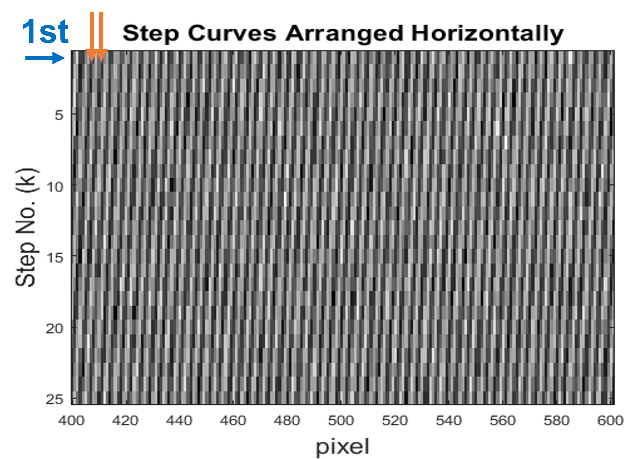
(a)

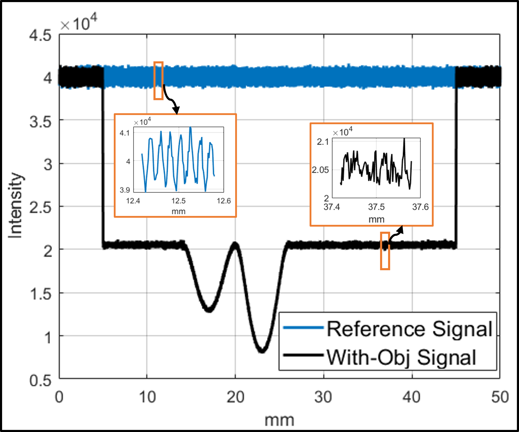
(b)

Figure 2: Stage 1 (a) Phase step curves arranged horizontally. The detector pixel size is $50\>\mu m$. Vertical raster scanning yields a single reference $I_{r}(x)$ at a stepping resolution of $2\>\mu m$ for this case. (b) ‘Reference’ signal, $I_{r}(x)$, and ‘object’ signal $I_{obj}(x)$, after rasterization for sampling recovery. However, at this stage, the visibility is low, only about $2\%$.

The second stage is the removal of the detector blur from the noisy reference image, $I_{r}(x)$, shown in Figure 3(a). Direct deconvolution produced oscillations and/or introduced apodization errors, so we performed this step iteratively, as is commonly done in super-resolution literature [26]. We aim to estimate a “clean” estimate of the reference image, $\hat{g}_{r}(x)$, that has no noise and no detector blur. This was done by iteratively fitting the initial parameters, [$\hat{A},\hat{B},\hat{\phi}_{0}$], where $\hat{\phi}_{0}$ is the phase of the initial reference pattern. While $\phi_{0}$ is not needed in the image simulation, real experimental data would have an arbitrary phase, so $\hat{\phi}_{0}$ must be included. Starting with an initial estimate, $\hat{g}_{r}(x)$ is calculated and detector blur is applied. The sum squared error (SSE) is calculated and minimized by iteratively updating [$\hat{A},\hat{B},\hat{\phi}_{0}$] using fmincon in Matlab until convergence is achieved.

The third stage, illustrated in Figure 3(b), is the recovery of $\mu T(x)$, $t_{ph}(x)$, and $S(x)$ by iterative reconstruction, using the ‘clean’ reference from Stage 1 in the forward model. A Poisson maximum likelihood model is used with adaptive gradient descent, summarized here. Starting with an initial estimate of $\mu T(x)$, $S(x)$ and $t_{ph}(x)$, the forward model is used to calculate the expected fringe pattern that contains no pixel blur or noise, $\hat{g}_{obj}(x)$, shown in Equation 5. The blur is then simulated by convolution, producing the expected measurement, $\hat{I}_{obj}(x)$. Note that $\hat{I}_{obj}(x)$ is simulated at the phase step resolution.

(a)

(b)

Figure 3: Stages 2 and 3 (a) Stage 2 to recover $\hat{g}_{r}$. This essentially recovers the visibility for the reference signal, $I_{r}(x)$. The recovered visibility was $18.4-19.6\%$ when the true visibility was $20\%$. (b) Stage 3 to recover $\mu T(x)$, $t_{ph}(x)$, and $S(x)$.

$$\hat{g}_{obj}(x)=\left\{\hat{A}e^{-S(x)}\cos\left(\frac{2\pi}{p_{D}}\left(x+t_{ph}(x)+\hat{\phi}_{0}\right)\right)+\hat{B}\right\}e^{-\mu T(x)}$$ (5)

$$\hat{I}_{obj}(x)=\hat{g}_{obj}(x)\star PSF(x)\star s(x)$$ (6)

This is used in combination with the rasterized measurement produced in Stage 1, $I_{obj}(x)$, to calculate the Poisson likelihood of each pixel, shown in Equation 7.

$$L(x)=I_{obj}(x)*\log{\left(\hat{I}_{obj}(x)\right)}-\hat{I}_{obj}(x)$$ (7)

The parameters are then updated using gradient descent, as shown in Equation 8, where $\theta_{i}(x)$ represents each parameter and $\lambda_{i}$ represents the learning rate of each parameter. If the average likelihood started to decrease, the learning rate was reduced by the adaption rate, $\eta>1$.

$$\theta_{i+1}(x)=\theta_{i}(x)+\lambda_{i}\frac{\partial L(x)}{\partial\theta_{i}(x)}$$ (8)

$$\lambda_{i+1}=\lambda_{i}/\eta\text{, if $\overline{L}$ decreases}$$ (9)

Since the function $L$ directly involves the oscillatory intensity, it is smoothed via convolution by a window of width $2p_{D}$ so that the $\theta$ estimates do not oscillate in x. In this method the parameters are fit one at a time, first $\mu T(x)$, then $t_{ph}(x)$, then $S(x)$. This is not unlike some of the standard methods of estimation where the three parameters are estimated more or less independently – with the attenuation estimated from zeroth-frequency information, while the small angle scatter is estimated from first harmonic after normalizing from attenuation effects.

2.3. Simulation Parameters

Table 1: TLI and MPGI setups that produce $p_{D}=22\>\mu m$ and $ACL=0.564\>\mu m$ $(D_{OD}=40\>cm)$. The visibility is before detector blur.

System	Source-to-Grating Distance	Grating-to-Detector Distance	Visibility
TLI	71 mm	710 mm	69.4%
MPGI	887 mm	1065 mm	53.6%

In this work, the simulations performed are system agnostic since the only required parameters for Equation 5 are the desired bias, visibility, fringe period, and step resolution. Geometries for two systems are shown in Figure 1 that both produce $p_{D}=22\>\mu m$ and $ACL=0.564\>\mu m$. The first system is a Talbot-Lau interferometer (TLI), with a $\pi$ phase grating at $40\>keV$ with $p_{1}=4\>\mu m$. The second system is a Modulated Phase Grating Interferometer (MPGI), with a $(\pi,0)$ RectMPG at $40\>keV$ with $W=10\>\mu m$ and $p_{x}=1\>\mu m$. The visibility shown was found by simulating the systems using our analytical Fresnel diffraction simulator [22] at $70\>kVp$ with a $1\>\mu m$ source before detector blur. Even though the visibility before detector blur was very high, we conservatively chose to use a visibility of $20\%$ in our simulations for simplicity and to account for some of the effects not simulated, such as the visibility loss due to Compton scatter. Images were simulated for a $30\>\mu m$ and $50\>\mu m$ detector with a box blur PSF. The simulations have an initial resolution of $1\>\mu m$, and the phase stepping is simulated at $2\>\mu m$ and $5\>\mu m$ resolution. The number of phase steps was equal to the pixel size divided by the step resolution.

The Poisson noise was simulated at levels determined by analyzing the signal-to-noise ratio (SNR) in previous experiments [23]. Due to calibration, the mean intensity could not be used due to a calibration scale factor. Therefore, we focused on the SNR = mean/std = $\sqrt{N}$ to arrive at the effective bias count, N. The measured SNR was approximately 200 for each phase step image. The images were taken under low-dose operation, with a Microfocus X-ray tube running at a $55\>\mu A$ current and $40\>kVp$ voltage for 20-second exposures. Therefore, we chose an initial bias of $N=40000$ for the case of n = 25, detector pixel 50 $\mu m$ and step resolution 2 $\mu m$.

We performed two analyses to compare the effects of noise and step resolution. The first set is known as the ‘same noise’ case, where the bias for each phase step is the same, meaning the noise level was similar across all instances of detector pixel size and step resolution. This means the net counts at each pixel (hence dose) increase with the number of phase steps, n. The second set is a ‘noise-adjusted’ case, where the total counts per pixel is held constant, regardless of the number of phase steps, and the bias of each phase step was adjusted. The bias was adjusted to keep the total counts the same as the aforementioned case of 25 phase steps, $50\>\mu m$ detector, and $2\>\mu m$ step resolution, which had a bias of $N=40000$ for each phase step, so a total counts of $10^{6}$. The counts (bias) of each phase step for each scenario is tabulated in Table 2.

We tested two phase step resolutions, $2\>\mu m$ and $5\>\mu m$, so the number of phase steps was $n=15$ and $n=6$ for the $30\>\mu m$ detector and $n=25$ and $n=10$ for the $50\>\mu m$ detector. The resolution limit set by the Nyquist theorem is determined by $p_{D}=22\>\mu m$. Since our reconstruction methods rasterize the phase steps to iteratively estimate the parameters, image recovery depends on the noise level of each phase step, just as in interferometry using traditional algorithms [34].

Table 2: Number of counts (bias) of each pixel per phase step for ‘same noise’ and ‘adjusted noise’ scenarios.

Pixel Size	No. of steps (n)	Set I: Counts/Step	Set II: Counts/Step
$30\>\mu m$	15 (step-res $2\>\mu m$)	40K	67K
	6 (step-res $5\>\mu m$)	40K	167K
$50\>\mu m$	25 (step-res $2\>\mu m$)	40K	40K
	10 (step-res $5\>\mu m$)	40K	100K

The object simulated is a virtual lung phantom with a thickness of $T=10\>cm$, with “tumor” and “non-tumor” regions. For the non-tumor region, an attenuation coefficient of $\mu=0.06675\>cm^{-1}$ was used, from the NIST XCOM database of lungs at $40\>keV$ [35]. In this region, multiple values of $S$ were simulated. $S=1$ was used to represent healthy lungs, found using the normalized dark-field coefficient of $R=1.5$ from [24]. $S=0.25$ was chosen to represent diseased lungs such as fibrosis or emphysema, which has been shown to produce reduced dark-field signal [4]. The real part of the index of refraction was $\delta=1.82\times 10^{-7}$, found by scaling the value from [36] from $33\>keV$ to $40\>keV$. Two apodized “tumors” were added with maximum thickness of $2.5\>cm$ and $5\>cm$. At their peak, the tumors have an attenuation coefficient of $\mu=0.25\>cm^{-1}$, produce no visibility loss due to SAXS, and $\delta=10^{-7}$. These values were chosen to best represent the effects of tumor tissue (higher density and no scatter). The tumors are incorporated into the virtual phantom by partially “replacing” lung tissue and leaving behind the rest of the lung. For example, the peak $\mu T$ for the $5\>cm$ tumor was 1.58. This comes from $5\>cm$ of tumor and $5\>cm$ of non-tumor tissue.

3. Results

We tested the algorithm for 16 cases: two detectors ($30\>\mu m$, $50\>\mu m$), two step resolutions ($2\>\mu m$,   $5\mu m$), two sets of noise (‘same noise’ and ‘adjusted noise’), and two mathematical phantoms with 10 cm thickness that each had tumors that were 2.5 and 5 cm in thickness, but had different values of S for the ‘non-tumor’ region (S = 0.25, S = 1). A selection of results are shown in Figures 4–6. Figure 4 shows the results for S = 1, ‘same noise’, and $2\>\mu m$ step resolution, comparing the effects of detector pixel size. Since this is the same noise case and the counts (bias) of each phase step are the same for both scenarios, the total X-ray dose is higher for the $50\>\mu m$ case. Figure 5 shows the results for S = 1, $50\>\mu m$ detector, and $5\>\mu m$ step resolution, comparing the ‘same noise’ and ‘adjusted noise’ cases. In this instance, the total X-ray dose is the same, but the ‘same noise’ case has more noise (lower bias per phase step). Figure 6 shows the results for S = 0.25, $5\>\mu m$ step resolution, ‘same noise’, and $5\>\mu m$ step resolution, comparing the effects of detector pixel size (similar to Figure 4, except S = 0.25 and using a $5\>\mu m$ step resolution).

(a) $30\mu m$ Detector, ‘same noise’ (40K)

(b) $50\mu m$ Detector, ‘same noise’ (40K)

Figure 4: Attenuation, differential-phase, and dark-field images for S = 1 (non-tumor region), 2 $\mu m$ step resolution, ‘same noise’ (40K) case (Table 2), and (a) 30 $\mu m$ detector pixels or (b) 50 $\mu m$ detector pixels.

(a) $50\mu m$ Detector, ‘same noise’ (40K)

(b) $50\mu m$ Detector, ‘adjusted noise’ (100K)

Figure 5: Attenuation, differential-phase, and dark-field images for S = 1 (non-tumor region), 5 $\mu m$ step resolution, 50 $\mu m$ detector pixels for the (a) ‘same noise’ (40K) case and (b) ‘adjusted noise‘ case (Table 2).

(a) $30\mu m$ Detector, ‘same noise’ (40K)

(b) $50\mu m$ Detector, ‘same noise’ (40K)

Figure 6: Attenuation, differential-phase, and dark-field images for S = 0.25 (non-tumor region), 5 $\mu m$ step resolution, ‘same noise’ (40K) case (Table 2), and (a) 30 $\mu m$ detector pixels or (b) 50 $\mu m$ detector pixels.

The mean value and RMSE from the constant region of the attenuation, differential-phase, and dark-field images (highlighted in cyan in Figures 4–6) for all 16 cases are tabulated in Tables 3 and 4. The RMSE captures the deviations of the mean from the true value and the deviations due to noise. We observe that the attenuation and differential-phase data are generally well fit, with the attenuation in particular having errors less than 1% in all cases. The dark-field images are fit well in most cases, but are typically noisier than the differential-phase images. The mean and RMSE of the constant region of the dark-field images are further displayed as a bar chart in Figure 7. There is not a significant difference in the mean for the 4 cases. As expected, the ‘adjusted noise’ (higher counts) case typically has lower RMSE than the ‘same noise’ case, except when they are similar in the (50 $\mu m$, 2 $\mu m$) case which was used as the reference for noise adjustment. It is also seen that the cases with 2 $\mu m$ step resolution generally have lower RMSE than for $5\>\mu m$, likely due to the better resolution relative to the fringe period, $22\>\mu m$.

Table 3: Mean attenuation thickness, differential-phase, and scattering parameter for a non-tumor region (shown in cyan in the figures) with $\boldsymbol{S=1}$, with RMSE values shown in the parenthesis. The fringe period was $p_{D}=22\>\mu m$.

Pixel Size Resolution Same Noise Noise Adjusted $\boldsymbol{\mu T}$ $\boldsymbol{t_{ph}}$ ($\boldsymbol{\mu m}$) S $\boldsymbol{\mu T}$ $\boldsymbol{t_{ph}}$ ($\boldsymbol{\mu m}$) S 30 $\mu m$ 2 $\mu m$ 0.667(0.002) -0.015(0.194) 0.998(0.060) 0.667(0.001) 0.029(0.173) 1.004(0.044) 30 $\mu m$ 5 $\mu m$ 0.667(0.003) 0.004(0.279) 0.998(0.084) 0.667(0.001) -0.043(0.301) 1.007(0.049) 50 $\mu m$ 2 $\mu m$ 0.667(0.002) 0.040(0.424) 1.009(0.099) 0.667(0.002) -0.114(0.587) 1.009(0.097) 50 $\mu m$ 5 $\mu m$ 0.667(0.003) 0.014(0.697) 0.994(0.139) 0.667(0.002) -0.037(0.715) 0.997(0.099) True value: 0.667 0 1 0.667 0 1

Table 4: Mean attenuation thickness, differential-phase, and scattering parameter for a non-tumor region (shown in cyan in the figures) with $\boldsymbol{S=0.25}$, with RMSE values shown in the parenthesis. The fringe period was $p_{D}=22\>\mu m$.

Pixel Size Resolution Same Noise Noise Adjusted $\boldsymbol{\mu T}$ $\boldsymbol{t_{ph}}$ ($\boldsymbol{\mu m}$) S $\boldsymbol{\mu T}$ $\boldsymbol{t_{ph}}$ ($\boldsymbol{\mu m}$) S 30 $\mu m$ 2 $\mu m$ 0.667(0.002) 0.012(0.115) 0.258(0.030) 0.667(0.001) 0.058(0.126) 0.251(0.020) 30 $\mu m$ 5 $\mu m$ 0.667(0.002) -0.003(0.186) 0.246(0.042) 0.667(0.001) 0.061(0.918) 0.257(0.027) 50 $\mu m$ 2 $\mu m$ 0.667(0.002) 0.044(0.210) 0.256(0.051) 0.667(0.002) 0.055(0.195) 0.244(0.047) 50 $\mu m$ 5 $\mu m$ 0.668(0.002) 0.027(0.282) 0.249(0.085) 0.667(0.002) 0.005(0.211) 0.259(0.047) True value 0.667 0 0.25 0.667 0 0.25

Figure 7: Summary of S fitting results for the constant ‘non-tumor’ region. The number above each bar shows the noise level from Table 2. The x-axis labels in parentheses indicate the detector pixel size and step resolution in $\mu m$.

4. Discussion

We demonstrated that super-resolution iterative reconstruction can recover radiographic attenuation, differential-phase, and dark-field images using simulated data with varying detector resolution and signal-to-noise ratios for analyzer-less grating systems. The quantitative comparison showed promising results: all three modalities are recoverable without the analyzer grating used in conventional Talbot-Lau X-ray interferometry.

Several improvements could be made to the super-resolution algorithm. If computational power is not an issue, the forward model could be improved by incorporating the Sommerfeld-Rayleigh Diffraction Integral (SRDI) for attenuation and phase simulations as done in our prior work [22, 21] and post-modeling of small angle X-ray scattering, where the $e^{-S}$ may be applied to the bias-subtracted signal, and the bias added back subsequently. However, this method is computationally expensive, particularly for a 2D case. The algorithm currently uses gradient descent, and depending on the noise level, adjustments to the learning rate or adaptation rate was required. This was likely because the gradient was noisy and oscillatory. The algorithm could likely be improved by adopting non-derivative approaches for optimizing the maximum likelihood objective function. Additionally, regularization could be included in the objective function to prevent fit parameter oscillation and noisy deviations. In stage 2, the reference signal was reconstructed using only three parameters (amplitude, bias, and phase), which allowed the use of fmincon in Matlab (Mathworks Inc, Natick MA). However, in reality these parameters can be spatially varying, since the visibility may not be constant across the face of the grating [23]. In this case, instead of fmincon, we can use the more general iterative method of Stage 3 to recover a spatially varying reference amplitude, bias, and phase.

The reconstruction method implemented here (particularly in Stage 3) can likely be used to improve image quality in cases where the detector pixel is small enough to follow the Nyquist criterion and super-resolution is not required (e.g. $p_{D}=120\>\mu m$ with a $30\>\mu m$ detector). In this situation, phase stepping of the detector and the rasterization of Stage 1 can still be applied to enhance resolution. The iterative reconstruction alone can recover the attenuation, differential-phase, and dark-field images and potentially outperform traditional recovery methods thanks to the explicit incorporation of system degradation (and potentially a noise model).

Even though translating the detector (hence a relative motion between detector and object) is optimal for obtaining sub-pixel resolution, we can also translate the grating to recover the parameters. In this case, the lung tissue parameters will maintain the original detector resolution and not achieve the sub-pixel resolution.

This work considered signals from a one-dimensional lung phantom. Future work includes extending the analysis to two-dimensional radiography, three-dimensional interferometric computed tomography, dose analysis, and experimental verification.

5. Conclusion

We have shown that super-resolution can be used to resolve attenuation, differential-phase, and dark-field images with grating interferometers with detectors that fail to meet the Nyquist sampling rate needed for traditional image recovery algorithms. For the Talbot-Lau Interferometer, this allows for the removal of the analyzer grating, reducing X-ray dose. For the Modulated Phase Grating Interferometer, this allows for the use of modulated phase gratings with lower envelope periods, increasing the autocorrelation length. We have shown that iterative reconstruction can be used to recover images of a lung phantom with multiple diseased regions with one-dimensional interferometry simulated data. We have shown that the methods presented can be used with various detector resolutions, fringe periods, and signal-to-noise ratios for cases where traditional algorithms can not be used.

6. Acknowledgments

This work is funded in part by NIH NIBIB Trail-blazer Award 1-R21-EB029026-01A1.

References

- [1] Florian T. Gassert et al. “X-ray Dark-Field Chest Imaging: Qualitative and Quantitative Results in Healthy Humans” PMID: 34427464 In Radiology 301.2, 2021, pp. 389–395 DOI: 10.1148/radiol.2021210963
- [2] M. Bech et al. “In-vivo dark-field and phase-contrast x-ray imaging” In Scientific Reports 3.1, 2013, pp. 3209 DOI: 10.1038/srep03209
- [3] Andre Yaroshenko et al. “Visualization of neonatal lung injury associated with mechanical ventilation using x-ray dark-field radiography” In Sci Rep 6, 2016, pp. 24269
- [4] A Velroyen et al. “Grating-based X-ray Dark-field Computed Tomography of Living Mice” In EBioMedicine 2.10, 2015, pp. 1500–1506
- [5] Zhentian Wang et al. “Non-invasive classification of microcalcifications with phase-contrast X-ray mammography” In Nature Communications 5.1, 2014, pp. 3797 DOI: 10.1038/ncomms4797
- [6] Arne Tapfer et al. “Experimental results from a preclinical X-ray phase-contrast CT scanner” In Proc Natl Acad Sci U S A 109.39, 2012, pp. 15691–15696
- [7] Kai Scherer et al. “Bi-Directional X-Ray Phase-Contrast Mammography” In PLOS ONE 9.5 Public Library of Science, 2014, pp. 1–7 DOI: 10.1371/journal.pone.0093502
- [8] Thomas Koehler et al. “Slit-scanning differential x-ray phase-contrast mammography: proof-of-concept experimental studies” In Med Phys 42.4, 2015, pp. 1959–1965
- [9] Dan Stutman, Thomas J Beck, John A Carrino and Clifton O Bingham “Talbot phase-contrast x-ray imaging for the small joints of the hand” In Phys Med Biol 56.17, 2011, pp. 5697–5720
- [10] Junji Tanaka et al. “Cadaveric and in vivo human joint imaging based on differential phase contrast by X-ray Talbot-Lau interferometry” Schwerpunkt: Röntgenbasierte Phasenkontrast Bildgebung In Zeitschrift für Medizinische Physik 23.3, 2013, pp. 222–227 DOI: https://doi.org/10.1016/j.zemedi.2012.11.004
- [11] Florian T Gassert et al. “Dark-field X-ray imaging for the assessment of osteoporosis in human lumbar spine specimens” In Front Physiol 14, 2023, pp. 1217007
- [12] Xiayun Zhao and David W. Rosen “Real-time interferometric monitoring and measuring of photopolymerization based stereolithographic additive manufacturing process: sensor model and algorithm” In Measurement Science and Technology 28, 2016 URL: https://api.semanticscholar.org/CorpusID:125660749
- [13] Adam J. Brooks et al. “Early detection of fracture failure in SLM AM tension testing with Talbot-Lau neutron interferometry” In Additive Manufacturing 22, 2018, pp. 658–664 DOI: https://doi.org/10.1016/j.addma.2018.06.012
- [14] V. Revol et al. “Sub-pixel porosity revealed by x-ray scatter dark field imaging” In Journal of Applied Physics 110.4, 2011, pp. 044912 DOI: 10.1063/1.3624592
- [15] Atsushi Momose et al. “Demonstration of x-ray Talbot interferometry” In Japanese Journal of Applied Physics 42.7 B Japan Society of Applied Physics, 2003, pp. L866–L868 DOI: 10.1143/jjap.42.l866
- [16] Atsushi Momose “Recent Advances in X-ray Phase Imaging” In Japanese Journal of Applied Physics 44.9R, 2005, pp. 6355 DOI: 10.1143/JJAP.44.6355
- [17] Franz Pfeiffer, Timm Weitkamp, Oliver Bunk and Christian David “Phase retrieval and differential phase-contrast imaging with low-brilliance X-ray sources” In Nature Physics 2.4, 2006, pp. 258–261 DOI: 10.1038/nphys265
- [18] F. Pfeiffer et al. “X-ray dark-field and phase-contrast imaging using a grating interferometer” In Journal of Applied Physics 105.10, 2009, pp. 102006 DOI: 10.1063/1.3115639
- [19] J. Dey et al. “Phase Contrast X-ray Interferometry”, US Patent 10,872,708, Dec 22, 2020
- [20] J. Dey et al. “Phase Contrast X-ray Interferometry”, US Patent 11,488,740 B2, Nov 1, 2022
- [21] Jingzhu Xu, Kyungmin Ham and Joyoni Dey “X-ray interferometry without analyzer for breast CT application: a simulation study” In Journal of Medical Imaging 7.2 SPIE, 2020, pp. 023503 DOI: 10.1117/1.JMI.7.2.023503
- [22] I. Hidrovo et al. “Neutron interferometry using a single modulated phase grating” In Review of Scientific Instruments 94.4, 2023, pp. 045110
- [23] Hunter Meyer et al. “Theoretical and experimental analysis of the modulated phase grating X-ray interferometer” In Scientific Reports 14.1, 2024, pp. 26780
- [24] Simon Spindler et al. “The choice of an autocorrelation length in dark-field lung imaging” In Scientific Reports 13.1, 2023, pp. 2731
- [25] M. Strobl “General solution for quantitative dark-field contrast imaging with grating interferometers” In Scientific Reports 4.1, 2014, pp. 7243 DOI: 10.1038/srep07243
- [26] S. Farsiu, M.D. Robinson, M. Elad and P. Milanfar “Fast and robust multiframe super resolution” In IEEE Transactions on Image Processing 13.10, 2004, pp. 1327–1344 DOI: 10.1109/TIP.2004.834669
- [27] Till Dreier, Niccolò Peruzzi, Ulf Lundström and Martin Bech “Improved resolution in x-ray tomography by super-resolution” In Appl. Opt. 60.20 Optica Publishing Group, 2021, pp. 5783–5794 DOI: 10.1364/AO.427934
- [28] B. Gutman et al. “Angular super-resolution retrieval in small-angle X-ray scattering” In Scientific Reports 10.16038, 2020 DOI: 10.1038/s41598-020-73030-2
- [29] Yujia Chen and Mark A. Anastasio “Properties of a Joint Reconstruction Method for Edge-Illumination X-ray Phase-Contrast Tomography” In Sensing and Imaging 19.1, 2018, pp. 7 DOI: 10.1007/s11220-018-0186-y
- [30] Qiaofeng Xu et al. “Investigation of discrete imaging models and iterative image reconstruction in differential X-ray phase-contrast tomography” In Opt. Express 20.10 Optica Publishing Group, 2012, pp. 10724–10749 DOI: 10.1364/OE.20.010724
- [31] Cheng-Ying Chou, Yin Huang, Daxin Shi and Mark A. Anastasio “Image reconstruction in quantitative X-ray phase-contrast imaging employing multiple measurements” In Opt. Express 15.16 Optica Publishing Group, 2007, pp. 10002–10025 DOI: 10.1364/OE.15.010002
- [32] S. Gogh et al. “Iterative phase contrast CT reconstruction with novel tomographic operator and data-driven prior” In PloS one 17.9, 2022 DOI: 10.1371/journal.pone.0272963
- [33] Masih Nilchian et al. “Fast iterative reconstruction of differential phase contrast X-ray tomograms” In Opt Express 21.5, 2013, pp. 5511–5528
- [34] S. Marathe et al. “Improved algorithm for processing grating-based phase contrast interferometry image sets” In Rev Sci Instrum 85.1, 2014, pp. 013704
- [35] Martin Berger et al. “XCOM: Photon Cross Section Database (version 1.2)” http://physics.nist.gov/xcom, 1999
- [36] M J Kitchen et al. “On the origin of speckle in x-ray phase contrast images of lung tissue” In Phys Med Biol 49.18, 2004, pp. 4335–4348