Friedlin-Wentzell solutions of discrete Hamilton Jacobi equations

Abstract.

We consider a sequence of finite irreducible Markov chains with exponentially small transition rates: the transition graph is a fixed, finite, strongly connected directed graph; the transition rates decay exponentially on a paramenter $N$ with a given rate that varies from edge to edge. The stationary equation uniquely identifies the invariant measure for each $N$, but at exponential scale in the limit as $N$ goes to infinity reduces to a discrete equation for the large deviation rate functional of the invariant measure, that in general has not an unique solution. In analogy with the continuous case of diffusions, we call such equation a discrete Hamilton-Jacobi equation. Likewise in the continuous case we introduce a notion of viscosity supersolutions and viscosity subsolutions and give a detailed geometric characterization of the solutions in terms of special faces of the polyedron of Lipschitz functions on the transition graph. This parallels the weak KAM theory in a purely discrete setting. We identify also a special vanishing viscosity solution obtained in the limit from the combinatorial representation of the invariant measure given by the matrix tree theorem. This gives a selection principle on the set of solutions to the discrete Hamilton Jacobi equation obtained by the Friedlin and Wentzell minimal arborescences construction; this enlights and parallels what happens in the continuous setting.

1. Introduction

The Freidlin and Wentzell theory (FW theory) [10] is a milestone in the theory of stochastic processes and develops a general framework for studying the small noise limit of diffusion processes. The language and techniques used are typical of Large Deviations Theory (LDT) and are strongly connected to other areas of mathematics, such as discrete mathematics, calculus of variations, and the theory of Hamilton-Jacobi (HJ) equations

The basic mathematical object of FW theory is a sample-path large deviation (LD) principle for the weak noise limit of a diffusion process. This is a cost functional defined on absolutely continuous trajectories, which plays the role of a classical action obtained by integrating a Lagrangian. Starting from the action, FW theory introduces the so-called Quasipotential, which is obtained by a suitable minimization of the dynamic action. In cases where the stochastically perturbed vector field has multiple stable minima, the construction of the quasipotential also involves a discrete optimization procedure. The invariant measure of the system satisfies an LD principle with a rate functional that coincides with the quasipotential. By classical variational arguments, the quasipotential solves a stationary HJ equation. The stationary HJ equations arising in the FW theory do not have a unique Viscosity solution, but the uniqueness of the LD rate functional of the invariant measure selects a special solution. This solution can be obtained directly by considering the small noise limit of the unique invariant measure, in the same spirit as the vanishing viscosity limit for HJ equations. These special solutions of the HJ equations, arising in the weak noise limit of diffusions, have been considered, for example, in [8, 11, 12, 13].

The FW theory has a basic structure that has been extended to generalized frameworks, both infinite-dimensional and finite-dimensional. In the discrete case of continuous-time Markov chains, the analogous framework is that of Markov chains with exponentially small transition rates, which are widely used and considered in statistical mechanics and metastability (see, for example, [15, 16, 20, 21, 22]). For Markov chains of this type, we have a sample-path LD principle and an LD principle for the invariant measure. Within the framework of large deviations theory, we introduce a discrete HJ equation that must be solved by the LD rate functional of the invariant measure of the chain. We introduce the notion of sub- and super-solutions, which allows us to identify solutions—i.e., functions that are both super- and sub-solutions—as points of the faces of the polytope of one-Lipschitz functions, with the appropriate dimensionality. A special solution is identified by the limit of the unique invariant measure, in the same spirit as the vanishing viscosity solutions. This special solution is constructed through a discrete optimization problem on rooted directed arborescences, which is the same optimization problem used to define the quasipotential in the continuous FW case with several stable equilibria. We note that our HJ equation is defined on any weighted directed graph without any other geometric structure. In particular, there is a natural action defined on paths obtained through an LD principle, but there is no corresponding natural Hamiltonian. It would be interesting to extend our constructions to metric graphs, where continuous arborescences play a role in the identification of the invariant measure, see [1], and a theory for HJ equations has been developed (see for example [5] and references therein). We also remark that the discrete Lax-Oleinik semigroup, which we introduce using our discrete action, is related to algorithms for shortest paths on directed graphs, such as Dijkstra’s or the Bellman-Ford-Moore algorithms, see [3].

In summary, we introduce a stationary discrete HJ equation on a finite directed weighted graph, which naturally arises from variational problems associated with the LD rate functional of Markov chains with exponentially small transition rates. We provide a detailed analysis of the structure of the viscosity solutions and identify a special solution obtained as the limit of the unique invariant measure. The discrete theory parallels the weak KAM theory and FW theory in the continuous setting. The discrete framework allows for a clearer view of formulas, constructions, and characterizations.

The paper is organized as follows:

Section 2 introduces our framework of continuous-time Markov chains with exponentially small transition rates, describes the basic assumptions, and derives a discrete HJ equation on abstract directed weighted graphs as a natural equation within LD theory.

Section 3 identifies a special solution of the discrete HJ equation using a combinatorial representation of the invariant measure in terms of directed arborescences. We call this solution the Freidlin–Wentzell solution.

Section 4 introduces the notion of viscosity solutions, describes special features in terms of the graph’s geometry, and demonstrates that the combinatorial solution is indeed a viscosity solution.

Section 5 explores the geometry of the set of viscosity solutions, identifying it with specific faces of the polyhedron of one-Lipschitz functions with particular dimensionality. We also introduce the notion of Quasipotentials and provide a general representation formula for viscosity solutions.

Section 6 briefly outlines a parallel with the weak KAM theory obtained from a sample path large deviations principle for the Markov chains.

Section 7 presents examples and identifies the FW solution as the vanishing viscosity solution.

2. The discrete Hamilton Jacobi equation

Let $\mathcal{G}=(V,E)$ be a finite, strongly connected directed graph, meaning that any two vertices can be connected by directed paths. Assume there are no loops, i.e., no edges of the form $(x,x)$. Consider a sequence of irreducible Markov chains with transition probabilities depending on a parameter $N$. Denote by $(r_{N}(x,y))_{(x,y)\in E}$ the rates of jumps from $x\in V$ to $y\in V$ with $(x,y)\in E$, and define $r_{N}(x):=\sum_{y:(x,y)\in E}r_{N}(x,y)$ as the total rate of jumps from $x\in V$.

Under these assumptions, the invariant measure is unique [14]. Furthermore, the stationarity condition characterizing the invariant measure $\pi_{N}$ is given by:

$$\pi_{N}(x)\sum_{y:(x,y)\in E}r_{N}(x,y)=\sum_{y:(y,x)\in E}\pi_{N}(y)r_{N}(y,x)\,,\qquad\forall x\in V\,.$$ (2.1)

We consider the case where the rates are exponentially small. Specifically, we assume that the following condition holds throughout the rest of the paper.

Assumption 2.1 (See [16]).

The rates of jump $(r_{N}(x,y))_{(x,y)\in E}$ are exponentially small with $N$, namely the following limits exist and are finite

$$\Delta(x,y):=-\lim_{N\to+\infty}N^{-1}\log r_{N}(x,y)\geq 0\,,\qquad\forall(x,y)\in E\,.$$

Define a sequence of functions $W_{N}$ by the relation $\pi_{N}(x)=:e^{-NW_{N}(x)}$, then equation (2.1) uniquely defines $(W_{N})_{N\in\mathbb{N}}$. The study of large deviations of $(\pi_{N})_{N\in\mathbb{N}}$ is related to the study of the limit of the sequence $(W_{N})_{N\in\mathbb{N}}$. The following lemma shows that the limit can be characterized as a solution of a discrete equation.

Lemma 2.2 (HJ equation).

Consider the sequence of probability measures $(\mu_{N})_{N\in\mathbb{N}}$ solutions to (2.1) and assume that there exist the limits

$$W(x):=-\lim_{N\to+\infty}N^{-1}\log\mu_{N}(x)\,,\qquad\forall x\in V\,.$$ (2.2)

Then $W$ satisfies the following set of equations

$$W(x)+\min_{y:(x,y)\in E}\left\{\Delta(x,y)\right\}=\min_{y:(y,x)\in E}\left\{W(y)+\Delta(y,x)\right\}\,,\qquad\forall x\in V\,.$$ (2.3)

Proof.

Since in (2.1) there are finite sums, considering $\lim_{N\to+\infty}\frac{1}{N}\log(\cdot)$ on both sides, using Assumption 2.1, by the basic principle of large deviations (”the largest exponent wins”, see for example [6] formulas I.1, I.2) equation (2.3) holds. ∎

This is precisely what occurs in the continuous case of diffusions, where the HJ equation is derived as the vanishing noise limit of the stationary equation, see [10]. In line with the classical FW theory for diffusions, we refer to the limiting equation (2.3) as a discrete Hamilton–Jacobi equation (discrete HJ equation).

It turns out that, unlike equation (2.1), the discrete HJ equation does not always admit a unique solution, as occurs in the continuous setting. An interesting feature of the discrete framework is that it allows for a detailed characterization of the set of solutions. To achieve this, we introduce an additional assumption.

(a) A graph $(V,E)$ satisfying Assumption 2.3. The edges with $\Delta$ equal to zero are highlighted in red.

(b) The corresponding subgraph $(V,E_{0})$.

Figure 1.

Assumption 2.3.

For any $x\in V$ there is exactly one $(x,y)\in E$ such that $\Delta(x,y)=0$. Call $E_{0}\subseteq E$ the set of edges $(x,y)\in E$ having $\Delta(x,y)$ equal to zero (Figure 1).

This assumption simplifies several geometric structures, enabling complete characterizations while preserving an interesting mathematical framework. In the general case, however, there may be more variations, making a full characterization of solutions to the discrete HJ equations more challenging.

By Assumptions 2.1 and 2.3, it follows that the function $W:V\to\mathbb{R}$ of Lemma 2.2 has to satisfy following discrete HJ equation

$$W(x)=\min_{y:(y,x)\in E}\left\{W(y)+\Delta(y,x)\right\}\,,\qquad\forall x\in V\,.$$ (2.4)

3. Freidiln-Wentzell solution

3.1. Graphs and notation

Some general remarkable classes of graphs and their properties are needed in order to discuss solutions to the discrete HJ equation.

Definition 3.1.

Let $\mathcal{G}$ be a directed graph. An arborescence $\tau\subseteq\mathcal{G}$ directed toward $x\in V$ is a spanning subgraph of $\mathcal{G}$ such that:

1) For each vertex $y\neq x$ there is exactly one directed edge exiting from $y$ and belonging to $\tau$.

2) For any $y\in V$ there exists a unique directed path from $y$ to $x$ in $\tau$.

3) There are no edges exiting from $x$.

Let $\mathcal{T}_{x}$ be the set of arborescences of $\mathcal{G}$ directed toward $x\in V$ and $\mathcal{T}$ be the set of all directed arborescences $\mathcal{T}=\cup_{x\in V}\mathcal{T}_{x}$.

If the graph is strongly connected, then clearly $\mathcal{T}_{x}$ is not empty for any $x\in V$.

Given a weight function $Q:E\to\mathbb{R}$, to any arborescence $\tau$ the following weights are associated

$$\left\{\begin{array}[]{l}Q(\tau):=\sum_{e\in\tau}Q(e)\,,\\ \mathcal{P}_{Q}(\tau):=\prod_{e\in\tau}Q(e)\,.\end{array}\right.$$ (3.1)

In the formulas above, the products and sums are taken over all directed edges $e$ that belong to the arborescence $\tau$. For example, if the weight function is $r_{N}$, then $\mathcal{P}_{r_{N}}(\tau)=\prod_{e\in\tau}r_{N}(e)$; and if the weight function is $\Delta$, then $\Delta(\tau)=\sum_{e\in\tau}\Delta(e)$. A similar notation is used for subgraphs that are not arborescences.

A cycle in $\mathcal{G}$ is a sequence $(z_{1},\dots,z_{n})$ of distinct vertices $z_{i}\in V$ such that $(z_{i},z_{i+1})\in E$ where $z_{n+1}\equiv z_{1}$ .

3.2. Invariant measures and the Matrix Tree Theorem

One of the primary goals of this paper is to establish a connection between the large deviations of the sequence $(\pi_{N}(x))_{x\in V}$, representing the invariant measures of the chains, and the discrete HJ equation. This aims to develop a discrete analogue of the classical FW framework for diffusions.

The unique invariant measure of an irreducible Markov chain has an interesting combinatorial representation. The Markov chain Matrix Tree Theorem claims that the invariant measure is given by

$$\pi_{N}(x)=\frac{\sum_{\tau\in\mathcal{T}_{x}}\mathcal{P}_{r_{N}}(\tau)}{\sum_{\tau\in\mathcal{T}}\mathcal{P}_{r_{N}}(\tau)}\,.$$ (3.2)

See, for example, [18], where you can also find an interpretation of (3.2) in terms of determinants. For the sake of completeness, the particularly elegant proof of the Markov chain Matrix Tree Theorem from [18] is outlined in the appendix.

The Matrix Tree Theorem allows for the immediate deduction of a large deviations principle for the sequence of invariant measures.

Lemma 3.2.

The sequence of invariant measures $(\pi_{N})_{N\in\mathbb{N}}$ defined in (3.2) satisfies a large deviations principle with rate functional

$$\mathscr{FW}(x):=\lim_{N\to+\infty}-\frac{1}{N}\log\pi_{N}(x)=\inf_{\tau\in\mathcal{T}_{x}}\Delta(\tau)-\inf_{\tau\in\mathcal{T}}\Delta(\tau)\,,\qquad x\in V\,.$$ (3.3)

The function $\mathscr{FW}$ is called $FW$-quasipotential and it is a solution to the discrete HJ equation (2.3).

Proof.

Formula (3.2) together with Assumption 2.1 implies immediately (again by the basic principle of large deviations ”the largest exponent wins”, see for example [6] formulas I.1, I.2) that the sequence $(\pi_{N})_{N\in\mathbb{N}}$ satisfies (3.3). The function $\mathscr{FW}:V\to\mathbb{R}^{+}$ is the LD rate functional of the invariant measure. By Lemma 2.2, $\mathscr{FW}$ is a solution of equation (2.3). Note that the additive constant in (3.3) implies that $\inf_{x\in V}\mathscr{FW}(x)=0$. ∎

4. Viscosity solutions

Observe that the discrete HJ equations (2.3) and (2.4) form a collection of equations that must be satisfied at each node of the graph. In general, this discrete HJ equation does not have a unique solution.

Solutions to (2.4) can be naturally characterized—similarly to viscosity solutions for continuous HJ equations—using subsolution and supersolution conditions.

Definition 4.1.

A function $W:V\to\mathbb{R}$ is a subsolution of equation (2.4) if the following inequality holds for all $(x,y)\in E$:

$$W(x)\leq W(y)+\Delta(y,x)\,,\qquad(x,y)\in E\,.$$ (4.1)

A function $W:V\to\mathbb{R}$ is a supersolution of (2.4) if, for any $x\in V$, there exists $y^{*}=y^{*}(x)\in V$ such that $(y^{*},x)\in E$ and

$$W(x)=W(y^{*})+\Delta(y^{*},x)\,,\qquad x\in V\,.$$ (4.2)

Let $E_{W}\subseteq E$ be the set of edges where equality (4.2) is verified and we call it the Skeleton of $W$. A function $W$ is a solution of (2.4) if it is both a subsolution and a supersolution.

Call $\underline{\mathcal{W}}$ and $\,\overline{\!\mathcal{W}}$ the set of subsolutions and supersolutions, respectively, and call $\mathcal{W}:=\underline{\mathcal{W}}\cap\,\overline{\!\mathcal{W}}$ the set of solutions.

Since adding an arbitrary constant to a solution leads to another solution, it is natural to consider the set of normalized solutions, which we refer to as

$$\mathcal{W}_{0}:=\left\{W\in\mathcal{W}:\inf_{x\in V}W(x)=0\right\}\,.$$ (4.3)

As already observed in the proof of Lemma 3.2, the $\mathscr{FW}$ solution belongs to $\mathcal{W}_{0}$.

4.1. Maps and unicyclic compontents

The following classes of subgraphs will be relevant for the characterization of the viscosity solutions of the discrete HJ equation.

Definition 4.2.

Let $\mathcal{G}$ be a directed graph. A Map $\mathfrak{f}$ is a spanning subgraph of $\mathcal{G}$ such that for each vertex $x\in V$ there exists exactly one edge $(x,y)\in\mathfrak{f}$ exiting from $x$.

The name is due to the fact that a map $\mathfrak{f}$ is encoded by an injective function $f:V\to V$ such that $\mathfrak{f}=\Big{(}V,(x,f(x))_{x\in V}\Big{)}$.

The last definition refers to subgraphs with only one cycle.

Definition 4.3.

A subgraph $\mathfrak{u}$ of a directed graph $\mathcal{G}$ is called an inward oriented unicyclic component, or simply in-unicyclic component, if

• there exists a unique directed cycle $C_{\mathfrak{u}}$ in $\mathfrak{u}$,

• for any vertex $x$ in $\mathfrak{u}$ that lies outside the cycle $C_{\mathfrak{u}}$, there is a unique edge in $\mathfrak{u}$ exiting $x$, and a directed path from $x$ to $C_{\mathfrak{u}}$.

A subgraph $\mathfrak{o}$ of a directed graph $\mathcal{G}$ is called an outward oriented unicyclic component, or simply out-unicyclic component, if

• there exists a unique directed cycle $C_{\mathfrak{o}}$ in $\mathfrak{o}$,

• for any vertex $x$ in $\mathfrak{o}$ that lies outside the cycle $C_{\mathfrak{o}}$, there is a unique edge in $\mathfrak{o}$ entering $x$, and there exists a directed path from $C_{\mathfrak{o}}$ to $x$.

A spanning in-(out-)unicyclic component $\mathfrak{u}(\mathfrak{o})$, i.e. one that contains all the vertices in $V$, is called a in-(out-)unicyclic graph. Call $\mathcal{U}^{\mathrm{in}}$ and $\mathcal{U}^{\mathrm{out}}$ the collection of all the in-unicyclic and out-unicyclic graphs, respectively. On a strongly connected graph $\mathcal{G}$, every node belongs to the cycle of at least one in-unicyclic graph and at least one out-unicyclic graph of $\mathcal{G}$. Call $\mathcal{U}_{x}^{\mathrm{in}}$ and $\mathcal{U}_{x}^{\mathrm{out}}$ the set of in-unicyclic and out-unicyclic graphs with $x$ belonging to the unique cycle.

Figure 2. An in-unicyclic component on the left and an out-unicyclic component on the right

The structure of maps is well known; refer, for example, to [17] for the following basic fact: every map is the spanning disjoint union of in-unicyclic components. In particular, every in-unicyclic graph is a map.

Moreover, note that if the orientation of all the edges in a map is reversed, the resulting graph will have exactly one edge entering each node, forming a spanning disjoint union of out-unicyclic components; conversely, for any spanning collection of disjoint out-unicyclic components, reversing the orientation of its edges produces a map.

By Assumption 2.3, the graph $(V,E_{0})$ is a map. Call $\mathcal{C}$ the set of cycles of the map $(V,E_{0})$, then $1\leq|\mathcal{C}|\leq\left\lceil\frac{|V|}{2}\right\rceil$ ($\lceil\cdot\rceil$ represents the integer part). The value one is obtained in the case of one in-unicyclic graph and the second bound follows since there are no loops (edges of the type $(x,x)$).

For any $C_{i}\in\mathcal{C}$, $i=1,\dots,|\mathcal{C}|$, call $\mathfrak{u}_{i}$ the associated in-unicyclic component of $(V,E_{0})$ whose vertices are the basin of attraction of $C_{i}$, i.e. the set of $x\in V$ such that $d(x,C_{i})=0$. For simplicity of notation we write also $i\in\mathcal{C}$ to denote the cycle $C_{i}$.

4.2. Charachterization of $\underline{\mathcal{W}}$ and $\,\overline{\!\mathcal{W}}$

4.2.1. The set of subsolutions $\underline{\mathcal{W}}$

A discrete pseudo quasimetric is a function $d:V\times V\to\mathbb{[}0,+\infty)$ that satisfies

• triangle inequality: $d(x,z)\leq d(x,y)+d(y,z)$, for any $x,y,z\in V$,

• point inequality: $d(x,x)=0$, for any $x\in V$.

It may be not symmetric, i.e. there may exist $x,y\in V$ such that $d(x,y)\neq d(y,x)$, and not separable, i.e. there may exist $x,y\in V$, with $x\neq y$, such that $d(x,y)=0$.

The weights $\Delta:E\to\mathbb{[}0,+\infty)$ induce on the graph $(V,E)$ a pseudo quasimetric $d$ defined as

$$d(x,y):=\inf_{\gamma_{x,y}\in\mathcal{R}_{x,y}}\Delta(\gamma_{x,y})\,,$$ (4.4)

where $\mathcal{R}_{x,y}$ is the set of directed paths $\gamma_{x,y}$ from $x$ to $y$: a directed path from $x$ to $y$ is given by $\gamma_{x,y}:=(x_{0},x_{1},\dots x_{n})$ such that $x_{i}\in V$, $(x_{i},x_{i+1})\in E$, for all $i$ and $x_{0}=x,x_{n}=y$. Call $\Delta(\gamma_{x,y})$ the length of the path $\gamma_{x,y}$ and observe that $d(x,y)=d(y,x)=0$ when $x,y$ belong to the same cycle in the map $(V,E_{0})$.

Given $U,S\subseteq V$, define

$$d(U,y):=\inf_{x\in U}d(x,y),\quad d(x,S):=\inf_{y\in S}d(x,y),\quad d(U,S):=\inf_{x\in U,y\in S}d(x,y)$$

the distance between a set and a vertex, a vertex and a set, and two sets, respectively.

Call respectively $\bar{\gamma}_{x,y},\bar{\gamma}_{U,y},\bar{\gamma}_{U,S}$ the geodetic paths achieving the minimum in the above definitions (one of the paths chosen arbitrarily in the case of several minimizers).

Given a vertex $x$, it belongs to the exiting basin of attraction of the cycle $C_{i}\in\mathcal{C}$ if $d(C_{i},x)\leq d(C_{j},x)$ for any $j\neq i$. In the case where there is equality among two or more cycles, the node $x$ is assigned to the basin of attraction of an arbitrary cycle among the minimizers.

Definition 4.4.

Call $\mathrm{Lip}_{1}$ the set of Lipschitz functions with Lipschitz constant one that are identified by the set of $|V|\times(|V|-1)$ inequalities

$$W(x)-W(y)\leq d(y,x)\,,\qquad\forall x,y\in V\,.$$ (4.5)

The following result links subsolutions and Lipschitz functions.

Lemma 4.5.

The set of subsolutions and the set of Lipschitz functions define the same polyedron, i.e. $\underline{\mathcal{W}}=\mathrm{Lip}_{1}$.

Proof.

Let $W$ be a subsolution and let $\gamma_{yx}=(y=x_{0},x_{1},\dots,x_{n}=x)$ be a path from $y$ to $x$. Observe that, for any $i$, $W(x_{i+1})-W(x_{i})\leq\Delta(x_{i},x_{i+1})$ and the left hand side of the sum over $i$ of this inequalities is telescopic. Inequality (4.5) follows by taking the infimum over all paths. Conversely if (4.5) holds then, for any $(y,x)\in E$,

$$W(x)-W(y)\leq d(y,x)\leq\Delta(y,x).$$

∎

Since a function in $\mathrm{Lip}_{1}$ must be constant along the cycles in $\mathcal{C}$, the space $\mathrm{Lip}_{1}$ is a $|V|-\sum_{C_{i}\in\mathcal{C}}(|C_{i}|-1)$ dimensional polyhedron.

Remark 4.6.

Every polyedron $\mathfrak{P}$ can be written as the Minkowski sum $\mathfrak{P}=\mathfrak{C}+\mathfrak{B}$, where $\mathfrak{C}$ is a convex cone and $\mathfrak{B}$ is a polytope, i.e. a bounded polyedron, see for example section 5.3 of [19]. In the case of $\mathrm{Lip}_{1}$, the cone $\mathfrak{C}$ is reduced to a single line corresponding to functions that are multiple of the identity. This characteristic is also inherited by the solutions of the discrete HJ equations. For this reason, we focus solely on the normalized solutions by adding a suitable constant function. We do not delve further into these discrete geometric features.

4.2.2. The set of super solutions $\,\overline{\!\mathcal{W}}$

Consider an out-unicyclic component $\mathfrak{o}$ such that its unique cycle is one of the cycles in $\mathcal{C}$ and define the function $\omega_{\mathfrak{o}}:V\to\mathbb{R}$ as follows:

• $\omega_{\mathfrak{o}}(x)=0$ for any $x$ in the unique cycle,

• $\omega_{\mathfrak{o}}(x)=0$ for any $x\not\in\mathfrak{o}$,

• the values of $\omega_{\mathfrak{o}}(x)$ for the remaining $x\in\mathfrak{o}$ are uniquely determined by the condition $\omega_{\mathfrak{o}}(a)-\omega_{\mathfrak{o}}(b)=\Delta(b,a)$, for any $(b,a)\in\mathfrak{o}$.

Define also the indicator function of the nodes belonging to an out-cyclic component ${1\mskip-5.0mu{\rm I}}_{\mathfrak{o}}:V\to\{0,1\}$ by fixing ${1\mskip-5.0mu{\rm I}}_{\mathfrak{o}}(x)=1$ when $x\in\mathfrak{o}$ and zero otherwise.

A collection $(\mathfrak{o}_{i})_{i\in I}$ of out-unicyclic components is called spanning if the cycle of each component $\mathfrak{o}_{i}$ is an element of $\mathcal{C}$, all the components are disjoint and each $x\in V$ belongs to one component.

Proposition 4.7.

A function $W:V\to\mathbb{R}$ is an element of $\,\overline{\!\mathcal{W}}$ the set of supersolutions of the Hamilton Jacobi equation (2.4), if and only if there exists a spanning collection of out-unicyclic components $(\mathfrak{o}_{i})_{i\in I}$ and some values of the parameters $(\lambda_{i})_{i\in I}$, with $\lambda_{i}\in\mathbb{R}$, such that

$$W=\sum_{i\in I}\left(\omega_{\mathfrak{o}_{i}}+\lambda_{i}{1\mskip-5.0mu{\rm I}}_{\mathfrak{o}_{i}}\right)\,.$$ (4.6)

Proof.

Consider a function $W$ as in (4.6). Note that the terms of the sum are functions with disjoint support. Since the collection $(\mathfrak{o}_{i})_{i\in I}$ is spanning, any $x\in V$ belongs to exactly one $\mathfrak{o}_{i}$ and for each $x\in\mathfrak{o}_{i}$ there is exactly one $(y,x)\in\mathfrak{o}_{i}$. By the disjoint support property we have $W(x)-W(y)=\omega_{\mathfrak{o}_{i}}(x)-\omega_{\mathfrak{o}_{i}}(y)=\Delta(y,x)$, so that the supersolution condition is satisfied at each $x\in V$.

Conversely suppose that $W$ is a supersolution. In the skeleton $E_{W}$ there is at least one edge entering on each vertex of $V$. For each vertex in $V$ remove arbitrarly from $E_{W}$ all but one edge entering. As discussed below definition 4.1, the resulting graph is a spanning collection of out-unicyclic components $(\mathfrak{o}_{i})_{i\in I}$. The corresponding cycles can be only the elements $C_{i}\in\mathcal{C}$ and there are no other cycles, indeed $W(x)=W(y)$ for each $x,y\in C_{i}$. Define $\lambda_{i}:=W(x)$, $x\in C_{i}$, $\forall i\in I$. Then, for vertex $z\in\mathfrak{o}_{i}$, $W(z)=\omega_{\mathfrak{o}_{i}}(z)+\lambda_{i}$ and since the supports are disjoint formula (4.6) holds. ∎

4.3. Freidlin-Wentzell solutions

In Lemma 3.2 we proved that $\mathscr{FW}$ is a solution of the discrete HJ equation (2.4). It is also interesting and non-trivial to deduce this fact directly by inserting $\mathscr{FW}$ in (2.3).

Proposition 4.8.

The $FW$-quasipotential in (3.3) is always an element of $\mathcal{W}_{0}$, the set of normalized solutions of (2.3).

Proof.

The validity of (2.3) is checked for each node. Fix $x\in V$ and let $y^{*}\in V$ be such that $(x,y^{*})\in E_{0}$ and $\tau^{*}\in\mathcal{T}_{x}$ be the minimal arborescence in (3.3). Then $\Delta(x,y^{*})=0$ and $\Delta(\tau^{*})$ is minimal in $\mathcal{T}_{x}$.

From the setup, $\gamma^{*}:=(x,y^{*})\cup\tau^{*}\in\mathcal{U}^{\mathrm{in}}_{x}$ and moreover

$$\Delta(\gamma^{*})=\min_{\gamma\in\mathcal{U}^{\mathrm{in}}_{x}}\Delta(\gamma)=\Delta(\tau^{*})\,.$$ (4.7)

In fact, any $\gamma\in\mathcal{U}^{\mathrm{in}}_{x}$ can be written as $\gamma=(x,y)\cup\tau$ for a suitable $y\in V$ and $\tau\in\mathcal{T}_{x}$ and $\Delta(\gamma)=\Delta(x,y)+\Delta(\tau)$. Since both $\Delta(x,y^{*})$ and $\Delta(\tau^{*})$ are minimal (respectively on $(x,y)\in E$ and $\mathcal{T}_{x}$) we proved (4.7).

For any $y\in V$ , up to a constant, $\mathscr{FW}(y)=\Delta(\tau)$ for a suitable $\tau\in\mathcal{T}_{y}$ and moreover when $(y,x)\in E$ the graph $(y,x)\cup\tau\in\mathcal{U}^{\mathrm{in}}_{x}$. By (4.7)

$$\mathscr{FW}(y)+\Delta(y,x)=\Delta((y,x)\cup\tau)\geq\Delta(\gamma^{*})=\mathscr{FW}(x)\,,\qquad\forall(y,x)\in E\,,$$ (4.8)

that means $\mathscr{FW}\in\underline{\mathcal{W}}$. It remains to prove that there exists an $(y^{\prime},x)\in E$ such that the equality holds in (4.8), i.e. $\mathscr{FW}\in\,\overline{\!\mathcal{W}}$. Consider $(y^{\prime},x)$ the unique edge entering in $x$ and belonging to the unique cycle in $\gamma^{*}\in\mathcal{U}^{\mathrm{in}}_{x}$ (recall that $\gamma^{*}$ is carachterized by (4.7)).

Since $\gamma^{*}\setminus(y^{\prime},x)\in\mathcal{T}_{y^{\prime}}$

$$\mathscr{FW}(y^{\prime})+\Delta(y^{\prime},x)\leq\Delta(\gamma^{*}\setminus(y^{\prime},x))+\Delta(y^{\prime},x)=\Delta(\gamma^{*})=\mathscr{FW}(x)\,.$$ (4.9)

Last inequality together with the inequality (4.8), implies the equality. ∎

5. The geometric structure of $\mathcal{W}$

In this section we give some general representations of the set of solutions of the discrete HJ equation and discuss their geometric characterizations.

5.1. Minimal solutions

Proposition 4.8 establishes that there exists at least one solution of (2.4). The following proposition indicates that if there are two or more solutions, they can be combined to form others.

Proposition 5.1.

Suppose that $\left\{W_{j}\right\}_{j\in J}\subseteq\mathcal{W}$ is a family of solutions of the discrete HJ equation (2.4). Then the function $W_{J}$, defined as

$$W_{J}(x):=\inf_{j\in J}\{W_{j}(x)\},\quad\forall x\in V.$$

is a solution of the discrete HJ equation. If moreover $\left\{W_{j}\right\}_{j\in J}\subseteq\mathcal{W}_{0}$ then $W_{J}\in\mathcal{W}_{0}$,

Proof.

For all $x\in V$:

$$\min_{y:(y,x)\in E}\left\{W_{J}(y)+\Delta(y,x)\right\} =\min_{y:(y,x)\in E}\left\{\inf_{j\in J}\Big{\{}W_{j}(y)\Big{\}}+\Delta(y,x)\right\}$$

$$=\min_{y:(y,x)\in E}\left\{\inf_{j\in J}\Big{\{}W_{j}(y)+\Delta(y,x)\Big{\}}\right\}$$

$$=\inf_{j\in J}\left\{\min_{y:(y,x)\in E}\Big{\{}W_{j}(y)+\Delta(y,x)\Big{\}}\right\}$$

$$=\inf_{j\in J}\Big{\{}W_{j}(x)\Big{\}}$$

$$=W_{J}(x).$$

The forth equality is obtained using that $W_{j}$ is solution for each $j\in J$. The second statement follows by the fact that $0\leq\inf_{x}W_{J}(x)\leq\inf_{x}W_{j}(x)=0$ so that $W_{J}\in\mathcal{W}_{0}$. ∎

Corollary 5.2.

The discrete HJ equation (2.4) admits among the normalized solution a minimal one, defined as

$$W_{m}:=\inf\left\{W:W\in\mathcal{W}_{0}\right\}.$$ (5.1)

Proof.

By Proposition 4.8, $W_{m}\in\mathcal{W}_{0}$ and, by definition, $W_{m}\leq W$ for any $W\in\mathcal{W}_{0}$. ∎

Proposition 5.1 can be easily extended to the solutions of the general discrete HJ equation (2.3).

5.2. Quasipotentials

For each subset $C$ of $V$, the distance between set $C$ and a node $x$ defines a function that measures the minimum cost to move from a node in $C$ to the node $x$. If $C$ is a cycle in $\mathcal{C}$ this function is a normalized solution to the discrete HJ equation.

Definition 5.3.

For each cycle $C\in\mathcal{C}$ of $(V,E_{0})$, define the corresponding quasipotential based on $C$ as

$$W_{C}(x):=d(C,x)\,,\qquad x\in V\,.$$ (5.2)

Observe that, by definition, $W_{C}(x)=0$ for any $x\in C$ and $W_{C}(x)>0$ for any $x\not\in C$.

Fix $C\in\mathcal{C}$ and consider the edges $\bar{\gamma}_{C}:=\cup_{\left\{x\in V\cap C^{c}\right\}}\bar{\gamma}_{C,x}$. Call $(V,\bar{\gamma}^{*}_{C})$, the directed graph obtained removing arbitrarily from $\bar{\gamma}_{C}$, for each node $x\not\in C$ all the entering edges except one and finally adding the edges of the cycle $C$.

Lemma 5.4.

The directed graph $(V,\bar{\gamma}^{*}_{C})=\mathfrak{o}$ is a spanning out-unicyclic graph with unique cycle $C$. Moreover, $W_{C}(x)=\omega_{\mathfrak{o}}(x)$.

Proof.

Since it is constructed using geodetic, the directed graph $(V,\bar{\gamma}^{*}_{C})$ has a unique cycle that is $C$ and, for each vertex $x\in V$ outside the cycle, there is exactly one edge entering to $x$, and this means that it is a spanning out-unicyclic component. The equality $W_{C}(x)=\omega_{\mathfrak{o}}(x)$ follows by definition. ∎

Proposition 5.5.

For each $C\in\mathcal{C}$ the quasipotential $W_{C}$ based on $C$ belongs to $\mathcal{W}_{0}$.

Proof.

By Proposition 4.7 and Lemma 5.4, $W_{C}$ is a supersolution. For the subsolution condition, suppose that there exists $(y,x)\in E$ such that $W_{C}(x)>W_{C}(y)+\Delta(y,x)$. By definition of $W_{C}$ previpus inequality is impossible when at least one among $x,y$ belong to $C$; we assume therefore that $x,y\not\in C$. Define the path $\tilde{\gamma}_{C,x}=\bar{\gamma}_{C,y}\cup(y,x)$. Then it follows that

$$d(C,x)=\Delta(\bar{\gamma}_{C,x})=W_{C}(x)>W_{C}(y)+\Delta(y,x)=\Delta\big{(}\tilde{\gamma}_{C,x}\big{)}\,,$$

which is impossible since $\bar{\gamma}_{C,x}$ is a geodetic from $C$ to $x$. The normalization follows since $W_{C}\geq 0$ and $W_{C}(x)=0$ for any $x\in C$. ∎

This is a special situation of a more general case when, given a collection of spanning out-unicyclic components $(\mathfrak{o}_{i})_{i\in I}$, for each $x\in\mathfrak{o}_{i}$ the unique path from the cycle $C_{i}$ to $x$ is a geodetic path $\,\overline{\!\gamma}_{C_{i},x}$. An out-unicyclic component of this type is called geodetic out-unicyclic component.

The following simple lemma will be useful for the characterization.

Lemma 5.6.

Take $V\in\mathcal{W}$. The associated family of spanning out-unicyclic components $(\mathfrak{o}_{i})_{i\in I}$ in Proposition 4.7 is composed by geodetic out-unicyclic components.

Proof.

Assume by contraddiction that $\mathfrak{o}_{i}$ is not geodetic. There exists an $x\in\mathfrak{o}_{i}\cap C_{i}^{c}$ whose path in $\mathfrak{o}_{i}$ from $C_{i}$ is not the geodetic one. This implies that $V(x)-V(y)>d(C_{i},x)$, with $y\in C_{i}$, and by Lemma 4.5, $V$ is not a subsolution. ∎

The following theorem gives a complete characterization of solutions of (2.4) in terms of the parameters $\lambda=(\lambda_{i})_{i\in\mathcal{C}}\in\mathbb{R}^{|\mathcal{C}|}$.

Theorem 5.7.

The set $\mathcal{W}$ of the solutions to the discrete HJ equation (2.4) coincides with the family of functions

$$W_{\lambda}=\min_{i\in\mathcal{C}}\Big{\{}W_{C_{i}}+\lambda_{i}\Big{\}}\,,$$ (5.3)

where the vector $\lambda=(\lambda_{i})_{i\in\mathcal{C}}$ belongs to the polyhedron $\mathrm{Lip}_{1}^{\mathcal{C}}$ in $\mathbb{R}^{|\mathcal{C}|}$ defined by

$$\lambda_{i}-\lambda_{j}\leq d(C_{j},C_{i})\,.$$ (5.4)

Proof.

For any $i$, $W_{C_{i}}+\lambda_{i}$ is a solution then, by Proposition 5.1, $W_{\lambda}$ it is also a solution for any $\lambda\in\mathbb{R}^{|\mathcal{C}|}$. It remains to show that every solution can be written as in formula (5.3) with $\lambda$ statisfying (5.4).

Take a solution $W\in\mathcal{W}$. Since $W$ is both a supersolution and subsolution, it can be written as (4.6) with $(\mathfrak{o}_{i})_{i\in I}$ a spanning geodetic out-unicyclic components. Since any solution has to be constant on each cycle in $\mathcal{C}$, adding all the edges of the cycles in $\mathcal{C}$ we can assume that the set of labels $I$ of the components concides with $\mathcal{C}$. We call $\lambda_{i}=W(x)$, where $x\in C_{i}$. Inequality (5.4) is then satisfied because $W$ is in $\mathrm{Lip}_{1}$:

$$\lambda_{i}-\lambda_{j}=W(x)-W(y)\leq d(y,x)=d(C_{j},C_{i}),$$

where $x\in C_{i}$ and $y\in C_{j}$. By definition we have $W(x)=W_{C_{i}}(x)+\lambda_{i}$ for any $x\in\mathfrak{o}_{i}$. The final step in the proof is to show that, for any $x\in\mathfrak{o}_{i}$ and $j\neq i$, it holds: $W_{C_{i}}(x)+\lambda_{i}\leq W_{C_{j}}(x)+\lambda_{j}$. Take $y\in C_{j}$. Since $W$ is subsolution, $W(x)-W(y)\leq d(C_{j},x)$ that is equivalent to $W(x)\leq\lambda_{j}+W_{C_{j}}(x)$.

∎

Observe now that the function $d$ induces a discrete quasimetric among the cycles $\mathcal{C}$ in $(V,E_{0})$ defined by $d(C,C^{\prime})$, for any $C,C^{\prime}\in\mathcal{C}$. Under the Assumption 2.3, the distance $d(C,C^{\prime})>0$, for any $C\neq C^{\prime}$. Condition (5.4) says that the parameters $(\lambda_{i})_{i\in\mathcal{C}}$ coincide with the set $\mathrm{Lip}_{1}^{\mathcal{C}}$ of the Lipschitz functions on $\mathcal{C}$ with respect to the quasimetric $d$.

The $\mathscr{FW}$ solution can be identified as a special solution of the form (5.3). Let $\mathscr{FW}^{\mathcal{C}}$ be the minimal weight of arborescences on the complete graph with vertices $\mathcal{C}$ and weights $d$. We have the following representation of the FW solution $\mathscr{FW}$

Proposition 5.8.

The solution $\mathscr{FW}$ in (3.3) corresponds to a solution as in (5.3) with $\lambda_{i}=\mathscr{FW}^{\mathcal{C}}(C_{i})$, i.e. we have

$$\mathscr{FW}(x)=\min_{C\in\mathcal{C}}\Big{\{}W_{C}(x)+\mathscr{FW}^{\mathcal{C}}(C)\Big{\}}.$$ (5.5)

Proof.

For $x\in C^{\prime}\in\mathcal{C}$, it is easy to show by contraddiction that the minimum in (5.5) is obtained for $C=C^{\prime}$. Moreover, by definition $W_{C^{\prime}}(x)=0$. We have then that, up to a constant, the right hand side of (5.5) coincides with $\mathscr{FW}$ on all the vertices belonging to the cycles in $\mathcal{C}$. Since by Theorem 5.7 the values $\lambda$ completely identify the solution, then the right hand side of (5.5) coincides with $\mathscr{FW}$. ∎

The above result implies that the minimal arborescence $\tau\in\mathcal{T}_{x}$ is obtained by joining minimal arborescences among the cycles in $\mathcal{C}$. It incurs zero cost for paths from vertices to the cycle of the basin of attraction and requires a single geodetic path $\gamma_{C^{\prime},x}$ for some $C^{\prime}\in\mathcal{C}$.

5.3. Faces of the polyhedron $\mathrm{Lip}_{1}$

We describe some features of the polyhedron $\mathrm{Lip}_{1}$, and identify the solutions of (2.4) with a subset of the relative boundary of such polyhedron.

The polyhedron $\mathrm{Lip}_{1}$ is identified by the inequalities (4.5), but as shown in Lemma 4.5 we can restrict to the inequalities $W(x)-W(y)\leq\Delta(y,x)$ for $(y,x)\in E$. Furthermore, the inequalities associated to edges such that $\Delta(y,x)>d(y,x)$ are redundant. The relative boundary of $\mathrm{Lip}_{1}$ is the region where at least one of the effective inequalities is indeed an equality. The relative boundary is the union of faces of different dimensions.

A face is identified therefore by the edges of $E$ where equality takes place and this means that to each face, there is an associated subgraph $\mathfrak{f}\subseteq\mathcal{G}$ that shares the same vertices of $\mathcal{G}$ and has special features. Of course equality has to be always satisfied on edges of the cycles in $\mathcal{C}$ so that for any $i$ we have $C_{i}\subseteq\mathfrak{f}$. A complete geometric carachterization of faces may be difficult: we have for example that any directed path on $\mathfrak{f}$ has to be a geodetic; we just identify some special faces. Let $g$ be a function belonging to a face in the relative boundary of $\mathrm{Lip}_{1}$ associated the subgraph $\mathfrak{f}$. Ignore the orientation of arrows in $\mathfrak{f}$; since equality takes place on edges, the values of $g$ on vertices belonging to the same connected component of the unoriented subgraph are completely determined by the value of one single vertex. This means that the dimension of the face corresponds to the number of components of the induced subgraph. This dimension can be decresead by one considering the invariance of the polyhedron by a global addition.

Consider $\mathfrak{f}=(\mathfrak{u}_{i})_{i\in\mathcal{C}}$, the collection of in-unicyclic components that are the basin of attaction of the cycles in $(V,E_{0})$. Note that any path in $\mathfrak{f}$ is geodetic and moreover each edge $e\in\mathfrak{f}$ is such that $\Delta(e)=0$. The subgraph $\mathfrak{f}$ has $|\mathcal{C}|$ components and corresponds to a special $|\mathcal{C}|$ dimensional face of $\mathrm{Lip}_{1}$ that contains all the functions $g$ that are constant on each basin of attraction $\mathfrak{u}_{i}$. The values $\lambda_{i}$ that the function $g$ assumes on each basin must satisfy (5.4). We call such face the minimal $|\mathcal{C}|$ face.

Consider now $\mathfrak{f}=(\mathfrak{o}_{i})_{i\in\mathcal{C}}$ a spanning collection of out-unyciclic geodetic components. Any subgraph $\mathfrak{f}$ of this type has $|\mathcal{C}|$ components and corresponds to a $|\mathcal{C}|$ dimensional face of $\mathrm{Lip}_{1}$. A function $g$ that belongs to one of such faces assumes the values $\lambda_{i}$ on the cycles in $\mathcal{C}$ and the values on all the remaining vertices in $\mathfrak{o}_{i}$ are completely determined by $(\lambda_{i})_{i\in\mathcal{C}}$. The values $(\lambda_{i})_{i\in\mathcal{C}}$ have to satisfy additional constraints with respect to (5.4), depending on the geometry of $\mathfrak{f}$; indeed there could also be in some cases no values of $(\lambda_{i})_{i\in\mathcal{C}}$. The new constraints arise from the fact that, fixing $(\lambda_{i})_{i\in\mathcal{C}}$, the function is naturally Lipschitz inside each component, but it is not guaranteed to be globally Lipschitz.. We call faces of this type maximal $|\mathcal{C}|$ faces.

Theorem 5.9.

The set $\mathcal{W}$ of the solutions of the Hamilton Jacobi equation (2.4) coincides with the union of the maximal $|\mathcal{C}|$ dimensional faces of the polyhedron $\mathrm{Lip}_{1}$. Moreover for any $\lambda=(\lambda_{i})_{i\in\mathcal{C}}\in\mathrm{Lip}_{1}^{\mathcal{C}}$ there exist, among the functions in $\mathrm{Lip}_{1}$ assuming the values $\lambda_{i}$ for all $C_{i}\in\mathcal{C}$, a minimal function $g_{m}$ and a maximal one $g_{M}$; moreover $g_{m}$ belongs to the minimal $|\mathcal{C}|$ dimensional face and $g_{M}$ belongs to a maximal $|\mathcal{C}|$ dimensional face and indeed coincides with $W_{\lambda}$.

Proof.

Given a solution $W\in\mathcal{W}$, the corresponding skeleton identifies the spanning outgoing geodetic family $(\mathfrak{o}_{i})_{i\in\mathcal{C}}$ of a $\mathfrak{f}$ that corresponds to a maximal $|\mathcal{C}|$ dimensional face of $\mathrm{Lip}_{1}$ to which $W$ belongs. Conversely given $W$ that belongs to a maximal $|\mathcal{C}|$ dimensional face identified by $\mathfrak{f}$, then: $W$ is a subsolution since is one Lipschitz and it is also a supersolution with the skeleton corresponding to the edges of $\mathfrak{f}$.

For the second part of the statement fix $\lambda\in\mathrm{Lip}_{1}^{\mathcal{C}}$. For any function $W\in\mathrm{Lip}_{1}$, for any $x\in V$ and for any $i\in\mathcal{C}$ we have $W(x)-\lambda_{i}\leq d(C_{i},x)$. This implies

$$W(x)\leq\inf_{i}\left\{\lambda_{i}+d(C_{i},x)\right\}=W_{\lambda}(x)\,.$$

The unique function $g_{m}$ that belongs to the minimal $|\mathcal{C}|$ dimensional face and assumes the values $\lambda$ on the cycles is the function that is constantly equal to $\lambda_{i}$ on each vertex of $\mathfrak{u}_{i}$ for any $i\in\mathcal{C}$. Since the one Lipschitz condition imposes that any function in $\mathrm{Lip}_{1}$ that takes the values $\lambda\in\mathrm{Lip}_{1}^{\mathcal{C}}$ on the cycles has necessarily to assume on $\mathfrak{u}_{i}$ a value bigger or equal to $\lambda_{i}$, for any $i$, the proof is complete. ∎

An interesting question is to find a useful geometric carachterization of $\mathscr{FW}$ as an element of the relative boundary of $\mathrm{Lip}_{1}$.

6. Discrete weak KAM theory

In this section, we briefly outline how the above results parallel the general structure of the so-called weak KAM theory (see, for example, [7, 9, 23], to which we refer for comparison) in a purely discrete setting.

The key step in establishing this correspondence is to prove a sample path large deviations principle. The corresponding rate functional plays the role of the action. Although it is not natural to identify a Lagrangian and a corresponding Hamiltonian, we can define a discrete-time Lax-Oleinik semigroup and develop the parallel analysis.

Call $(X_{N}(t))_{t\in[0,T]}$ a trajectory of the Markov chain with parameter $N$ that is an element the Skorokhod space $D([0,T],V)$. An element $X=(X(t))_{t\in[0,T]}\in D([0,T],V)$ is determined by the number of jumps, $n\in\mathbb{N}$, the jumps times, $0<t_{1}<\dots<t_{n}<T$, and the values assumed, $(x_{0},x_{1},\dots,x_{n})\in V$. The trajectory $X$ is given by

$$X(t)=\sum_{i=0}^{n}x_{i}{1\mskip-5.0mu{\rm I}}_{[t_{i},t_{i+1})}(t)\,,t\in[0,T)\,,$$ (6.1)

where ${1\mskip-5.0mu{\rm I}}_{A}$ is the charachteristic function of set $A$, $t_{0}:=0$, $t_{n+1}:=T$, and we recall that $n=n(X)$ is the number of jumps of the trajectory. We have the following sample path large deviations principle.

Proposition 6.1.

The sequence of processes $\{(X_{N}(t))_{t\in[0,T]}\}_{N}$ satisfies a sample path large deviations principle on $D([0,T],V)$ with speed N and rate functional

$$\mathcal{A}_{[0,T]}(X)=\sum_{i=0}^{n(X)}\Delta(x_{i},x_{i+1})\,.$$ (6.2)

Proof.

Avoiding topological details, the result is obtained by splitting the trajectory space $D([0,T],V)=\cup_{n}D_{n}([0,T],V)$ into set of trajectories with exactly $n$ jumps. On $D_{n}([0,T],V)$, the probability density of $X_{N}$ on the coordinates $(x_{0},\dots,x_{n},t_{1},\dots,t_{n})$ is

$$\prod_{i=0}^{n}r_{N}(x_{i},x_{i+1})e^{-r_{N}(x_{i})(t_{i+1}-t_{i})}dt_{1}\dots dt_{n}\,,$$ (6.3)

where $r_{N}(x):=\sum_{y:(x,y)\in E}r_{N}(x,y)$. Given an open ball $B_{X}(\delta)$ centered on the trajectory $X$ and radius $\delta$, we have by Laplace Theorem that

$$\lim_{N\to+\infty}\frac{1}{N}\log\mathbb{P}_{X(0)}\left(X_{N}\in B_{X}(\delta)\cap D_{n}((0,T],V)\right)=-\inf_{Y\in B_{X}(\delta)\cap D_{n}((0,T],V)}\mathcal{A}_{[0,T]}(Y)\,,$$

this is because in (6.3) the term $\prod_{i=0}^{n}r_{N}(x_{i},x_{i+1})$ is exponentially small and gives the correct rate functional. A full LDP principle can be deduced by adding some topological details. ∎

The functional (6.2) acts as an action, assigning a cost to every trajectory of the system. An interesting feature of the action (6.2) is that it does not depend on the parameter $T$. For this reason, even though the stochastic dynamics are in continuous time, it is natural to define a corresponding discrete-time Lax-Oleinik semigroup.

Given a function $\mathcal{V}_{0}:V\to\mathbb{R}$ we define an iterated function $\mathcal{V}_{n}$ at time $n$ as

$$\mathcal{V}_{n}(x_{n}):=\inf_{x_{0},\dots,x_{n-1}}\left\{\mathcal{V}_{0}(x_{0})+\sum_{i=0}^{n-1}\Delta(x_{i},x_{i+1})\right\}=\inf_{y}\left\{\mathcal{V}_{n-1}(y)+\Delta(y,x_{n})\right\}\,.$$ (6.4)

This defines our discrete-time Lax-Oleinik semigroup. The fixed points of (6.4) are the solutions of the discrete HJ equation (2.4). This framework is natural for our discrete setting, as there is no straightfowrward definition of the Hamiltonian corresponding to the action (6.2).

Based on the definition (6.4), we note that our discrete contructions parallel the weak KAM theory, including discrete versions of all the related machinery and geometric constructions. We do not provide a detailed comparison here.

7. Examples and remarks

7.1. The reversible case

As an example, we consider the reversible case: in this situation, if $(x,y)\in E$ then also $(y,x)\in E$. The detailed balance characterizing the invariant measure $\pi_{N}$ in the reversible case is given by

$$\pi_{N}(x)r_{N}(x,y)=\pi_{N}(y)r_{N}(y,x)\,,\qquad(x,y)\in E\,.$$ (7.1)

The equivalent of Lemma 2.2 for the equation (7.1) gives the conditions

$$W(x)+\Delta(x,y)=W(y)+\Delta(y,x),\quad(x,y)\in E.$$ (7.2)

Equations (7.2) have a unique solution (up to an arbitrary additive constant) if the following condition, called gradient condition, is satisfied: $\delta(x,y):=\Delta(x,y)-\Delta(y,x)$ is a discrete vector field of gradient type, namely antisymmetric $\delta(x,y)=-\delta(y,x)$. If the rates are reversible (i.e. (7.1) is satisfied) the gradient condition is satisfied and there is a unique solution to (7.2); if the gradient condition is not satisfied there are clearly no solutions to (7.2).

The gradient condition corresponds to requiring that, for any cycle $C=(x_{0},\dots,x_{n})$, it holds $\sum_{(x,y)\in C}\delta(x,y)=0$. In this case the unique, up to an arbitrary constant, solution to (7.2) is

$$\mathscr{FW}(x):=\sum_{e\in\gamma_{x^{*},x}}\delta(e)\,,\forall x\in V,$$ (7.3)

where $x^{*}$ is an arbitrary fixed node and $\gamma_{x^{*},x}$ is also an arbitrary path. We used the notation $\mathscr{FW}$ since (7.3) coincides, up to a constant, with the Freidlin-Wentzell solution. Moreover, $\mathscr{FW}(y)-\mathscr{FW}(x)=\sum_{e\in\gamma_{x,y}}\delta(e)$.

In the reversible case the Assumption 2.3 imposes a strict condition on the graph $(V,E_{0})$.

Lemma 7.1.

Given a sequence of reversible Markov chains, Assumption 2.3 imposes that the map $(V,E_{0})$ contains only cycles of length 2, i.e. $|C|=2$ for any $C\in\mathcal{C}$.

Proof.

Consider $C\in\mathcal{C}$. Recalling the gradient condition and the fact that $\Delta(e)=0$ for $e\in C$, we have

$$0=\sum_{e\in C}\delta(e)=-\sum_{e\in C}\Delta(-e)\,,$$

where $-e$ is the edge obtained from $e$ by switching its orientation. The above equalities can be true only if $\Delta(e)=\Delta(-e)=0$ for any $e\in C$ but this implies that for each node in $C$ there are at least two edges in $E_{0}$ unless $|C|=2$. ∎

Figure 3. The switch of orientation from an arborescence oriented toward $x$ to an arborescence oriented toward $y$.

Remark 7.2.

In the reversible case, there is a bijection between $\mathcal{T}_{x}$ and $\mathcal{T}_{y}$ for any $x,y\in V$. The map from elements in $\mathcal{T}_{x}$ to $\mathcal{T}_{y}$ involves inverting the orientation of the edges in the unique directed path from $y$ to $x$ in $\mathcal{T}_{x}$. Similarly, the inverse map involves inverting the orientation of the edges in the unique path from $y$ to $x$ in $\mathcal{T}_{y}$ (see Figure 3).

Proposition 7.3.

The minimal weight arborescences ${\mathcal{\tau}}^{*}_{x}\in{\mathcal{T}}_{x}$ and ${\mathcal{\tau}}^{*}_{y}\in{\mathcal{T}}_{y}$ are related by the bijection in remark 7.2. In particular all the minimal weights arborescences $({\mathcal{\tau}}^{*}_{z})_{z\in V}$ have the same unoriented support, differ just by the orientation and $\Delta\left({\mathcal{\tau}}^{*}_{y}\right)-\Delta\left({\mathcal{\tau}}^{*}_{x}\right)=\sum_{e\in\gamma_{x,y}}\delta(e)$.

Proof.

Given ${\mathcal{\tau}}_{x}\in{\mathcal{T}}_{x}$ and ${\mathcal{\tau}}_{y}\in{\mathcal{T}}_{y}$ two elements linked by the bijection, by definition, we have

$$\Delta\left({\mathcal{\tau}}_{y}\right)-\Delta\left({\mathcal{\tau}}_{x}\right)=\sum_{e\in\gamma_{x,y}}\delta(e)=\mathscr{FW}(y)-\mathscr{FW}(x).$$ (7.4)

This implies that the weights of the arborescences in $\mathcal{T}_{y}$ are the same as those in $\mathcal{T}_{x}$, up to a global shift, and the minimizers are therefore mapped bijectively. Consequently, every pair of minimizers in $(\mathcal{T}_{z})_{z\in V}$ is related simply by the inversion of some arrows. The last statement follows from the fact that (7.4) holds for any pair of arborescences related by the bijection. ∎

In the reversible case, we can characterize the maximal $|\mathcal{C}|$ dimensional face to which the Friedlin Wentzell solution belongs. Recall that a maximal $|\mathcal{C}|$ dimensional face is indentified by a spanning collection of geodetic out-unicyclic components.

Proposition 7.4.

In the reversible case the solution $\mathscr{FW}$ belongs to the maximal $|\mathcal{C}|$ dimensional face of $\mathrm{Lip}_{1}$ associated to the spanning out-unicyclic geodetic components obtained reversing all the edges of the map $(V,E_{0})$.

Proof.

We need to show that the skeleton of $\mathscr{FW}$ is obtained by reversing the edges in $(V,E_{0})$. Recall that $\mathscr{FW}$ solves (7.2), then for any $(x,y\in E)$ we have

$$\mathscr{FW}(x)+\Delta(x,y)=\mathscr{FW}(y)+\Delta(y,x)\,.$$

Fix $x\in V$ and consider the infimum over all $y$ such that $(x,y)\in E$ of the left hand side of the above equation. We have that the minimum is achieved for the unique $(x,y^{*})\in E_{0}$. This leads to the equality $\mathscr{FW}(x)=\mathscr{FW}(y^{*})+\Delta(y^{*},x)$ which is equivalent to say that $(y^{*},x)$ belongs to the skeleton of $\mathscr{FW}$. ∎

7.2. The ring

Consider $\mathcal{G}$ as a finite ring with $k$ nodes , where $V=\mathbb{Z}/(k\mathbb{Z})$ and $E=\{(x,x\pm 1),x\in V\}$. In this case, we have a simple and compact representation of the $\mathscr{FW}$ solution, which shares a similar structure with the continuous one, see [8]. Let $\delta:E\to\mathbb{R}$ be the discrete vector field, i.e. such that $\delta(x,y)=-\delta(y,x)$, defined by $\delta(x,x+1):=\Delta(x,x+1)-\Delta(x+1,x)$, with the remaining values defined by antisymmetry. Define the function $S:\mathbb{N}\to\mathbb{R}$ by setting $S(x):=\sum_{y=1}^{x-1}\delta(y,y+1)$. In the previous formulas the function $\delta$ is computed on edges of $\mathcal{G}$ so that the sums in the arguments are modulo $k$ and $y+k=y$. If $S(k+1):=\sum_{y=1}^{k}\delta(y,y+1)=0$ we have that $S(y+k)=S(y)$ so that $S$ is a periodic function of period $k$, and this corresponds to the reversible case (since the gradient condition is satisfied).

We have

$$\mathscr{FW}(x)=\min_{x\leq y<x+k}\Big{\{}S(x)-S(y)-\Delta(y,y+1)\Big{\}}\,.$$ (7.5)

The function $\mathscr{FW}$ defined in (7.5) is defined on $\mathbb{N}$ but can be easily shown to be periodic of period $k$ so that can be naturally interpreted as a function on $V$. To prove that (7.5) coincides with (3.3) up to a constant, we have just to add and subtract on the right hand side of (7.5) the constant $\sum_{z=1}^{k}\Delta(z,z+1)$, getting that the right hand side of (7.5) coincides with $\min_{\tau\in\mathcal{T}_{x}}\left\{\Delta(\tau)-\mathbb{\sum}_{z=1}^{k}\Delta(z,z+1)\right\}$.

In the reversible case, when $S$ is periodic, we may write

$$\mathscr{FW}(x)=S(x)+\min_{x\leq y<x+k}\Big{\{}-S(y)-\Delta(y,y+1)\Big{\}}\,.$$

The second term on the right hand side does not depend on $x$ so that $\mathscr{FW}$ coincides with $S$ up to an additive constant.

The minimization formula (7.5) is very similar to the corresponding continuous one for diffusions on a circle and features a simple and interesting geometric interpretation, as in [8]. In the continuous case it is easier to describe but in the discrete setting there is a similar construction. Consider $f$ a continuous function on the unit circle $\mathbb{R}/\mathbb{Z}$ and define the function $S:\mathbb{R}\to\mathbb{R}$ as $S(x):=\int_{0}^{x}f(y)dy$. Taking

$$\mathscr{FW}(x):=\inf_{y\in[x,x+1]}\Big{\{}S(x)-S(y)\Big{\}}\,,$$ (7.6)

then Theorem 2.3 in [8] summarize some general properties of the function $\mathscr{FW}$, including the fact that it is one-periodic, i.e. it is a function on the circle, coincides with $S$ up to an additive constant if $\int_{0}^{1}f(y)dy=0$, and can be practically constructed by the so called sunshine transformation (see figure 4).

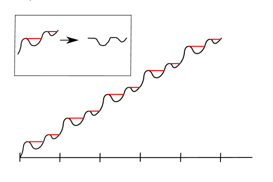
Figure 4. An example of the sunshine transformation for the case of a continuous function $S$ (in black) with $\int_{0}^{1}f(y)dy>0$. The light is assumed to arrive horizontally from the left; parts of the graph below the horizontal red line are in shadow, while the remaining parts are illuminated. The sunshine transformation retains the shadowed parts of the graph and replace the illuminated parts with horizontal segments, shifting them vertically to ensure that the final transformed graph remains continuous. An example of this transformation is illustrated on a portion of the graph inside the rectangle at the upper left. The transformed graph is periodic of period one. In the case $\int_{0}^{1}f(y)dy<0$, the construction is performed with the light arriving horizontally from the right. For $\int_{0}^{1}f(y)dy=0$, the graph is already periodic, every point of the graph is in shadow, and the transformation does not modify the graph.

Formula (7.6) can be interpreted as a minimal continuous arborescences construction, as suggested by the remark 1 in [8]. For the definitions of continuous arborescences on metric graphs and a continuous version of the Matrix Tree Theorem for diffusions on metric graphs, we refer to [1]. In the case of the continuous ring, a continuos arborescence directed torward a point $x$ is obtained cutting the ring on another point, say $y$, and orienting the two portions of the segment identified by $x$ to direct torward $x$. Formula (7.6) coincides up to an additive constant with

$$\mathscr{FW}(x)=\min_{y\in[x,x+1]}\Big{\{}\int_{x}^{y}[-f(z)]_{+}dz+\int_{y}^{x+1}[f(z)]_{+}dz\Big{\}}$$ (7.7)

where $[\cdot]_{+}$ is the positive part. This suggests that solutions of HJ equations associated to diffusions on metric graphs can be obtained by continuous minimal arborescences constructions.

7.3. Vanishing viscosity solutions

In the continuous setting, viscosity solutions of HJ equations can be obtained by a vanishing viscosity limit. In the case of a diffusion process on a ring, see for example [10, 8], the stationary HJ equation associated to the rate functional of the invariant measure is

$$H(x,W_{x})=W_{x}(W_{x}-f(x))=0\,.$$ (7.8)

In general, the viscosity solution of (7.8) is not unique and a natural selection principle for a solution is to consider the stochastic process behind and look at (7.8) as a limit of the stationary Kolmorogov equation. This means to consider the small noise limit $\varepsilon\to 0$ of the stationary condition

$$\varepsilon\left(e^{-\varepsilon^{-1}W^{\varepsilon}(x)}\right)_{xx}-\left(f(x)e^{-\varepsilon^{-1}W^{\varepsilon}(x)}\right)_{x}=0\,.$$ (7.9)

The unique smooth solution $W^{\varepsilon}$ can be found explicitely and converges, in the limit as $\varepsilon$ goes to zero, to the solution (7.6), i.e. $W^{\varepsilon}\to\mathscr{FW}$. The same solution is selected by the classic vanishing viscosity limit obtained by considering the equation

$$H(x,W^{\varepsilon}_{x})=W^{\varepsilon}_{x}\left(W^{\varepsilon}_{x}-f\right)=\varepsilon W^{\varepsilon}_{xx}\,.$$ (7.10)

Indeed, the unique smooth solution of the previous equation can be computed explicitely by the change of variables $\psi^{\varepsilon}=1/W_{x}^{\varepsilon}$ that linearizes the equation, and then it can be shown that again $W^{\varepsilon}\to\mathscr{FW}$.

We observe that the solution $\mathscr{FW}$ to the discrete HJ equation (2.4) can also be considered a vanishing viscosity solution. The stationary condition (2.1) written substituting $e^{-NW^{N}}$ to $\pi_{N}$ can be written as

$$e^{-NW^{N}(x)}\sum_{y:(x,y)\in E}r_{N}(x,y)=\sum_{y:(y,x)\in E}e^{-NW^{N}(y)}r_{N}(y,x)\,,\qquad\forall x\in V\,$$ (7.11)

By Lemma 3.2 we have that $\lim_{N\to+\infty}W^{N}=\mathscr{FW}$.

7.4. Two dimensional case

In this subsection we show how the FW-solution is an inner point of the polytope identified by $\mathcal{W}$.

Take $V=\{1,2,3,4\}$ and let $E$ be the set of edges depicted in figure 7.4. Suppose that $\Delta(1,2)=\Delta(2,1)=\Delta(3,4)=\Delta(4,3)=0$ and that, without loss of generality, $0<\Delta(2,3)<\Delta(4,1)$. The graph $(V,E_{0})$ contains two cycles, $C_{1}$ and $C_{2}$.

By Theorem 5.7 there exists a pair $(\lambda_{1},\lambda_{2})\in\mathrm{Lip}_{1}^{2}$ such that any solution to the discrete HJ equation (2.4) can be written as

$$W_{\lambda}(x)=\min\{W_{C_{1}}(x)+\lambda_{1};W_{C_{2}}(x)+\lambda_{2}\},$$

where

$$\begin{array}[]{r|cccc}&1&2&3&4\\ \hline\cr W_{C_{1}}&0&0&\Delta(2,3)&\Delta(2,3)\\ W_{C_{2}}&\Delta(4,1)&\Delta(4,1)&0&0\end{array}$$

The FW-solution is given by

$$\mathscr{FW}(1)=\mathscr{FW}(2)=\Delta(4,1)-\Delta(2,3);\qquad\mathscr{FW}(3)=\mathscr{FW}(4)=0.$$

By a straightforward calculation, we obtain that taking $\lambda_{1}=\Delta(4,1)-\Delta(2,3)$ and $\lambda_{2}=0$, we have $W_{\lambda}=\mathscr{FW}$. This choice of parameters shows that the FW-solution is indeed an inner point of the polytope identified by the normalized solution $\mathcal{W}_{0}$, see figure 7.4.

The grey area in figure 7.4 is the set $\mathrm{Lip}_{1}^{2}$ and $\mathcal{W}_{0}$ is indicated by the thiker segments on the axis.

Appendix A Lifting Markov chains

A simple and elegant way of proving the Markov chain tree Theorem is provided in [2] by constructing a Markov chain on an enlarged state space, such that its projection is the original Markov chain on $(V,E)$ with rates $r_{N}$. In particular we consider the directed graph $\widehat{\mathcal{G}}=(\mathcal{T},\widehat{E})$. The set of vertices coincides with the set of arborescences and $(\tau,\tau^{\prime})\in\widehat{E}$ if and only if $\tau\in\mathcal{T}_{x}$, $\tau^{\prime}\in\mathcal{T}_{y}$, $(x,y)\in E$ and the arborescence $\tau^{\prime}$ is obtained by $\tau^{\prime}=\left[\tau\cup(x,y)\right]\setminus(y,z)$ where $(y,z)$ is the unique edge exiting form $y$ in $\tau$. The rates $\widehat{r}_{N}$ of $(\tau,\tau^{\prime})\in\widehat{E}$ with $\tau\in\mathcal{T}_{x}$ and $\tau^{\prime}\in\mathcal{T}_{y}$ are given by $\widehat{r}_{N}(\tau,\tau^{\prime}):=r_{N}(x,y)$. Call $\widehat{X}_{N}$ the Markov chain associated to such rates. There is a natural projection map $\Pi:(\mathcal{T},\widehat{E})\to(V,E)$ such that, for any $\tau\in\mathcal{T}_{x}$, $\Pi(\tau)=x$ and, for any $(\tau,\tau^{\prime})\in\widehat{E}$ with $\tau\in\mathcal{T}_{x}$ and $\tau^{\prime}\in\mathcal{T}_{y}$, $\Pi(\tau,\tau^{\prime})=(x,y)$.

Theorem A.1.

[2] The Markov chain $\widehat{X}_{N}$ is irreducible, and has an unique invariant measure given by

$$\widehat{\pi}_{N}(\tau)=\frac{1}{Z_{N}}\mathcal{P}_{r_{N}}(\tau)\,,$$ (A.1)

where $Z_{N}$ is a normalization factor and the symbol $\mathcal{P}$ has been defined in (3.1). The process $X_{N}:=\Pi\left(\widehat{X}_{N}\right)$, is a Markov chain on $(V,E)$ with transition rates $r_{N}$ and we deduce (3.2) as a consequence.

Proof.

We give a sketch of the proof. The irreducibility of the Markov chain $\widehat{X}_{N}$ is discussed in [2]. The graph $(\mathcal{T},\widehat{E})$ is Eulerian since, for each node $\tau$ there is a bijection among outgoing and ingoing edges. Indeed, for each $\tau\in\mathcal{T}_{x}$, the outgoing edges in $\widehat{\mathcal{G}}$ are in correspondence with the outgoing edges from $x$ in $\mathcal{G}$. Let $\tau\in\mathcal{T}_{x}$ and $(\tau,\tau^{\prime})\in\widehat{E}$ with $\tau^{\prime}\in\mathcal{T}_{y}$. We have that $\tau\cup(x,y)=\mathfrak{u}_{x}\in\mathcal{U}^{\mathrm{in}}_{x}$ so that there exists $\tau^{\prime\prime}\in\mathcal{T}_{z}$ such that $\tau^{\prime\prime}\cup(z,x)=\tau\cup(x,y)=\mathfrak{u}_{x}$. This correspondence $(\tau,\tau^{\prime})\leftrightarrow(\tau^{\prime\prime},\tau)$ gives the bijection among exiting and entering edges at $\tau$, i.e. a bijection between exiting and entering elements of $\widehat{E}$ on each $\tau\in\mathcal{T}$ (see [4] section 2.6 for more details). Moreover by (A.1) we have, up to a common multiplicative constant,

$$\widehat{\pi}_{N}(\tau)r_{N}(x,y)=\widehat{\pi}_{N}(\tau^{\prime\prime})r_{N}(z,x)=\mathcal{P}_{r_{N}}(\mathfrak{u}_{x})\,.$$ (A.2)

Using the fact that the graph $(\mathcal{T},\widehat{E})$ is Eulerian, the stationarity of (A.1) follows. The last statements of the theorem are direct consequences of the definitions. ∎

Acknowledgements

M.A. acknowledges the Gruppo Nazionale per l’Analisi Matematica, la Probabilità e le loro Applicazioni (GNAMPA) of the Istituto Nazionale di Alta Matematica (INdAM). GP acknowledges the Gruppo Nazionale per la Fisica Matematica (GNFM) of the Istituto Nazionale di Alta Matematica (INdAM). DG acknowledges A. Faggionato, M. Mariani and Y. Shu for several useful discussions and the financial support from the Italian Research Funding Agency (MIUR) through PRIN project “Emergence of condensation-like phenomena in interacting particle systems: kinetic and lattice models”, grant n. 202277WX43.

References

- [1] Aleandri M., Colangeli M., Gabrielli D. A combinatorial representation for the invariant measure of diffusion processes on metric graphs ALEA Lat. Am. J. Probab. Math. Stat. 18(2021), no.2, 1773–1799.
- [2] Anantharam V.,Tsoucas P. A proof of the Markov chain tree theorem, Statistics and Probability Letters 8 (1989), no. 2, 189–192
- [3] Bang-Jensen J., Gutin G. Digraphs. Theory, algorithms and applications. Second edition. Springer Monographs in Mathematics. Springer-Verlag London, Ltd., London, 2009.
- [4] Biane P., Chapuy G. Laplacian matrices and spanning trees of tree graphs. Ann. Fac. Sci. Toulouse Math. (6) 26 (2017), no. 2, 235–261.
- [5] Camilli F., Marchi C. A comparison among various notions of viscosity solution for Hamilton-Jacobi equations on networks, J. Math. Anal. Appl. 407 (2013), no. 1, 112–118.
- [6] den Hollander F. Large deviations Fields Inst. Monogr., 14 American Mathematical Society, Providence, RI, 2000.
- [7] Evans L.C. Weak KAM theory and partial differential equations, Calculus of variations and nonlinear partial differential equations Lecture Notes in Math. 1927, Springer, Berlin, (2008), pp. 123–154.
- [8] Faggionato A., Gabrielli D. A representation formula for large deviations rate functionals of invariant measures on the one dimensional torus Ann. Inst. Henri Poincaré Probab. Stat. 48, (2012), no.1, 212–234.
- [9] Fathi A. Weak kam theorem in lagrangian dynamics to appear in Cambridge Studies in Advanced Mathematics.
- [10] Freidlin M.I., Wentzell A.D. Random perturbations of dynamical systems. Third edition. Grundlehren der mathematischen Wissenschaften, 260. Springer, Heidelberg, 2012.
- [11] Gao Y., Liu J.G. A selection principle for weak KAM solutions via Freidlin-Wentzell large deviation principle of invariant measures SIAM J. Math. Anal. 55 (2023), no.6, 6457–6495.
- [12] Graham R., Tel T. Weak-noise limit of Fokker-Planck models and nondifferentiable potentials for dissipative dynamical systems Phys. Rev. A 31, 1109 (1985).
- [13] Jauslin H. R. Nondifferentiable potentials for nonequilibrium steady states Physica A 144, 179 (1987).
- [14] Norris, J. R. Markov Chains Cambrige University Press (1997)
- [15] Olivieri E., Scoppola E. Markov chains with exponentially small transition probabilities: first exit problem from a general domain. I. The reversible case. J. Statist. Phys. 79 (1995), no. 3-4, 613–647.
- [16] Olivieri E., Scoppola E. Markov chains with exponentially small transition probabilities: first exit problem from a general domain. II. The general case. J. Statist. Phys. 84 (1996), no. 5-6, 987–1041.
- [17] Pitman J. Combinatorial stochastic processes. Lectures from the 32nd Summer School on Probability Theory held in Saint-Flour, July 7–24, 2002. With a foreword by Jean Picard. Lecture Notes in Mathematics, 1875.
- [18] Pitman J., Tang, W. Tree formulas, mean first passage times and Kemeny’s constant of a Markov chain. Bernoulli, 24 (3), 1942–1972 (2018).
- [19] Schrijver A. Combinatorial optimization. Polyhedra and efficiency. Vol. A. Paths, flows, matchings. Chapters 1–38, Algorithms Combin., 24,A Springer-Verlag, Berlin, 2003.
- [20] Scoppola E. Renormalization group for Markov chains and application to metastability. J. Statist. Phys. 73 (1993), no. 1-2, 83–121.
- [21] Scoppola E. Metastability for Markov chains: a general procedure based on renormalization group ideas. Probability and phase transition (Cambridge, 1993), 303–322, NATO Adv. Sci. Inst. Ser. C: Math. Phys. Sci., 420, Kluwer Acad. Publ., Dordrecht, 1994.
- [22] Scoppola E. Renormalization and graph methods for Markov chains. Advances in dynamical systems and quantum physics (Capri, 1993), 260–281, World Sci. Publ., River Edge, NJ, 1995.
- [23] Tran H.V. Hamilton-Jacobi equations—theory and applications. Grad. Stud. Math., 213, American Mathematical Society, (2021).