Identification of Nonparametric
Dynamic Causal Structure and
Latent Process in Climate System

Abstract

The study of learning causal structure with latent variables has advanced the understanding of the world by uncovering causal relationships and latent factors, e.g., Causal Representation Learning (CRL). However, in real-world scenarios, such as those in climate systems, causal relationships are often nonparametric, dynamic, and exist among both observed variables and latent variables. These challenges motivate us to consider a general setting in which causal relations are nonparametric and unrestricted in their occurrence, which is unconventional to current methods. To solve this problem, with the aid of 3-measurement in temporal structure, we theoretically show that both latent variables and processes can be identified up to minor indeterminacy under mild assumptions. Moreover, we tackle the general nonlinear Causal Discovery (CD) from observations, e.g., temperature, as a specific task of learning independent representation, through the principle of functional equivalence. Based on these insights, we develop an estimation approach simultaneously recovering both the observed causal structure and latent causal process in a nontrivial manner. Simulation studies validate the theoretical foundations and demonstrate the effectiveness of the proposed methodology. In the experiments involving climate data, this approach offers a powerful and in-depth understanding of the climate system.

1 Introduction

In real-world observations, such as weather data, video, and economic investigations, are often partially observed. Estimating latent variable causal graphs from these observations is particularly challenging, as the latent variables are in general not identifiable or unique due to the possibility of undergoing nontrivial transformations (Hyvärinen & Pajunen, 1999), even when the independent factors of variation are known (Locatello et al., 2019). Several studies have aimed to uncover causally-related latent variables in specific cases. For instance, (Silva et al., 2006) identified latent variables in linear-Gaussian models using Tetrad conditions (Spearman, 1928), while the Generalized Independent Noise (GIN) condition (Xie et al., 2020) has been proposed to estimate linear, non-Gaussian latent variable causal graphs. Recent work employs rank constraints to identify hierarchical latent structures (Huang et al., 2022). However, these approaches are constrained by linear relations and require specific types of structural assumptions.

Furthermore, nonlinear Independent Component Analysis (ICA) has established identifiability results using auxiliary variables (Hyvarinen & Morioka, 2016; 2017; Hyvärinen et al., 2023), showing that independent factors can be recovered up to a certain transformation of the underlying latent variables under appropriate assumptions. In contrast, Zheng et al. (2022); Zheng & Zhang (2023) develop identifiability results without auxiliary variables, relying instead on a sparse structure in the generating process, while Gresele et al. (2021) impose restrictions on the function classes of generating process. The framework of nonlinear ICA has been extended to address the identification of latent causal representations, a significant research focus (Schölkopf et al., 2021). For instance, with incorporating temporal structures, (Yao et al., 2022; lachapelle2024nonparametric) leverage time-lagged dependencies to model dynamic causal mechanisms, and Lippe et al. (2022) propose a framework for identifying latent variables in both time-lagged and instantaneous settings. Additionally, considering with multiple distributions, Yao et al. (2023) explore scenarios with partially observed variables, Buchholz et al. (2024) examine interventional data under linear mixing assumptions, and Zhang et al. (2024) introduce the theoretical guarantees for recovering latent moral graph in presence of environmental changes. However, most prior work assumes that the generating processes from latent variables to observations are deterministic, except for a few studies that consider linear additive noise (Khemakhem et al., 2020; Hälvä et al., 2021; Gassiat et al., 2020)—let alone scenarios where causal relations exist among observations. Moreover, all of the aforementioned work is constrained by the assumption of an invertible and deterministic generating function, which is often considered infeasible in many real-world scenarios.

A typical setting where such methodological assumptions are too restrictive is the climate system. With high-level latent variables dynamically changing and influencing observations (e.g., temperature, humidity) and causal structure (e.g., wind system), this presents a challenging problem that necessitates developing a solution to uncover these complex relationships. As a graphical depiction shown in Figure 1, the high-level climate variables—sunshine, CO2 (Stips et al., 2016), ocean currents (Paulson & Simpson, 1981), and rainfall (Chen & Wang, 1995)—are not directly observed. These variables evolve together through a temporal causal process, changing gradually and exhibiting causal relationships across both instantaneous and time-lagged interactions (Runge et al., 2019; Runge, 2020). This dynamic interplay reshapes their influence on temperature, human activities, and wind patterns. Moreover, regional temperatures interact via wind-driven heat transfer, which is influenced by latent variables and human activities (Vautard et al., 2019). Given these properties, we know that the climate is a forced and dissipative nonlinear system featuring non-trivial dynamics of a vast range of spatial and temporal scales (Lucarini et al., 2014; Rolnick et al., 2022), which traditional causal models are inadequate for capturing.

To address it, we focus on a temporal causal structure involving dynamic latent variables driving a latent causal process and causally-related observed variables, with all connections represented through general nonlinear functions. The final objective is to identify these factors under minimal indeterminacy. For this challenging task, we address three fundamental questions: (i) What unique attributes of latent variables can be recovered from the causally-related observed variables with the aid of temporal structures? (ii) How to do causal discovery in the presence of latent variables, without relying on conventional restrictions? (iii) How can empirically identify both the latent processes and the observed causal structure simultaneously? Towards tackling these questions, our main contributions are mainly three-fold:

1. We theoretically establish the conditions required for achieving the identifiability of latent variables from causally-related observations in a 3-measurement model.

2. We propose a functional equivalence that bridges nonlinear Structural Equation Models (SEMs) and nonlinear ICA models, and, guided by this principle, establish identifiability guarantees for observed causal Directed Acyclic Graphs (DAGs).

3. Building on these theoretical foundations, we present a comprehensive estimation framework that, to the best of our knowledge, is the first to simultaneously tackle CRL and CD. Extensive experiments on diverse synthetic and real-world datasets validate the effectiveness of our theory and methodology.

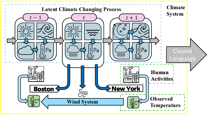
Figure 1: (Left) Systematic analysis of the climate system. (Center) Data generating process depicted by the climate system. (Right) 3-measurement model in the temporal data.

2 Problem Setup

Notations.

We conceptualize the data-generating process through the lens of our perspective on the climate system. It consists of observed variables $\mathbf{x}_{t}:=(x_{t,i})_{i\in\mathcal{I}}$ with index set $\mathcal{I}=\{1,2,\ldots,d_{x}\}$ and their causal graph $\mathcal{G}_{x_{t}}$. Additionally, there are latent variables $\mathbf{z}_{t}:=(z_{t,j})_{j\in\mathcal{J}}$ indexed by $\mathcal{J}=\{1,2,\ldots,d_{z}\}$ with the corresponding instantaneous causal graph $\mathcal{G}_{z_{t}}$. We assume no selection effects, so samples are drawn i.i.d. from the distribution. Let $\mathbf{pa}(\cdot)$ denote the parent variables, $\mathbf{pa}_{O}(\cdot)$ represent the parent variables in the observed space, and $\mathbf{pa}_{L}(\cdot)$ indicate the parent variables in the latent space. Notably, $\mathbf{pa}_{L}(z_{t,j})$ includes latent variables in current time step $t$ and previous time step $t-1$ that are parents of $z_{t,j}$. Specifically, we assume no time-lagged causal relationships in the observed space, and that future states cannot influence the past (Freeman, 1983). We use the hat symbol (e.g., $\hat{\mathbf{x}}_{t}$) to indicate estimated variables and functions, and the dot symbol (e.g., $\dot{\mathbf{x}}_{t}$ and $\ddot{\mathbf{x}}_{t}$) to denote a specific instance of a variable.

We first formally define the 3-measurement model, and describe how observed variables and latent variables are causally-related in data generating process by a structural equation model (SEM) (Spirtes et al., 2001; Pearl, 2009) in a general manner.

Definition 2.1 (3-Measurement Model)

$\mathbf{Z}=\{\mathbf{z}_{t-1},\mathbf{z}_{t},\mathbf{z}_{t+1}\}$ represents latent variables in three distinct states, where each state is indexed by its respective time step, we discretize it as $t\in\mathcal{T}=\{2,\ldots,T-1\}$ and $T\geq 3$. These latent states mutually influence one another. Similarly, $\mathbf{X}=\{\mathbf{x}_{t-1},\mathbf{x}_{t},\mathbf{x}_{t+1}\}$ are observed variables that directly measure $\mathbf{z}_{t-1},\mathbf{z}_{t},\mathbf{z}_{t+1}$ using the same generating functions $g$, while $\mathbf{x}_{t-1}$ and $\mathbf{x}_{t+1}$ provide indirect measurements of $\mathbf{z}_{t}$. Let $\mathcal{X}\subseteq\mathbb{R}^{d_{x}}$ denotes the range of $\mathbf{x}_{t}$, and $\mathcal{Z}\subseteq\mathbb{R}^{d_{z}}$ denote that of $\mathbf{z}_{t}$, where $d_{z}\leq d_{x}$. The model is defined by the following properties:

• The mapping between $\mathbf{z}_{t-1},\mathbf{z}_{t},\mathbf{z}_{t+1}$ is does not preserve the measure.

• Joint density of $\mathbf{x}_{t-1},\mathbf{x}_{t},\mathbf{x}_{t+1},\mathbf{z}_{t}$ is a product measure w.r.t. the Lebesgue measure on $\mathcal{X}_{t-1}\times\mathcal{X}_{t}\times\mathcal{X}_{t+1}\times\mathcal{Z}_{t}$, and a dominating measure $\mu$ is defined on $\mathcal{Z}_{t}$.

• $\mathbf{x}_{t-1},\mathbf{x}_{t}$ and $\mathbf{x}_{t+1}$ are conditional indepedent given $\mathbf{z}_{t}$.

Explanation.

The example in Figure 1 defines $\mathbf{x}_{t-1},\mathbf{x}_{t},\mathbf{x}_{t+1}$ as 3 different measurements of $\mathbf{z}_{t}$ within a temporal structure. This definition relies on the property of conditional independence, which is commonly assumed in causality (Spirtes et al., 2001; Pearl, 2009; Schölkopf et al., 2021).

Intuition behind 3-measurement.

As shown in Figure 1, climate time-series data satisfied the 3-measurement model, which supports the enough information for identification of latent variables, analogous to the needs in sufficient number of environments: domain changes in multiple distribution (Hyvärinen et al., 2023; Hyvarinen et al., 2019; Khemakhem et al., 2020; Zhang et al., 2024), sufficient variability in temporal structure (Yao et al., 2021; 2022; Chen et al., 2024), and enough pure children (Silva et al., 2012; Kong et al., 2023; Ng et al., ; Huang et al., 2022). The assumption of 3-measurement implies the minimum information required by Hu & Schennach (2008). If more than 3 measurements are available for the same latent variables, the additional measurements, which also carry information about the latent variables, typically enhance their recovery.

Definition 2.2 (Data Generating Process)

For $x_{t,i}\in\mathbf{x}_{t}$ and $z_{t,j}\in\mathbf{z}_{t}$, the data generating process is defined as follows:

$$x_{t,i}=g_{i}(\mathbf{pa}_{O}(x_{t,i}),\mathbf{pa}_{L}(x_{t,i}),s_{t,i});\quad z_{t,j}=f_{j}(\mathbf{pa}_{L}(z_{t,j}),\epsilon_{z_{t,j}});\quad s_{t,i}=g_{s_{i}}(\mathbf{z}_{t},\epsilon_{x_{t,i}}),$$ (1)

where $g_{i}$ and $f_{j}$ are differentiable functions, and $\epsilon_{z_{t,j}}\sim p_{\epsilon_{z_{j}}}$ are independent noise terms. The noise $s_{t,i}$ depending on $\mathbf{z}_{t}$ is modeled by a nonlinear generation from $\mathbf{z}_{t}$ and independent noise $\epsilon_{x_{t,i}}\sim p_{\epsilon_{x_{i}}}$.

We present a graphical depiction of the data-generating process in Figure 1. The causal relations within $\mathbf{x}_{t}$ highlight a fundamental divergence from previous works in causal representation learning (Zhang et al., 2024; Gresele et al., 2021; Schölkopf et al., 2021). We present a common assumption used in causal models as follows.

Assumption 2.3

The distribution over $(\mathbf{X},\mathbf{Z})$ is Markov and faithful to a DAG.

Compared with existed CD settings.

Extending our analysis of climate systems, the formulation for generating $x_{t,i}$ in the function space is more general than existing formulations employed in function-based causal discovery methods, including the post-nonlinear model (Zhang & Hyvarinen, 2012), nonlinear additive models (Ng et al., 2022; Rolland et al., 2022; Hoyer et al., 2008), nonlinear additive models with latent confounders (Zhang et al., 2012; Ng et al., ), and models with changing causal mechanisms and nonstationarity (Huang et al., 2020; 2019). Our framework is designed to address real-world climate scenarios characterized by general nonlinear causal relationships and latent variables. It encompasses the settings described above while enabling dynamic control over causal edges and generated effects through different subsets of latent variables and parameters.

3 Main Results

We present theoretical results showing that the block-wise information of latent causal variables can be recovered from causally related observations. Furthermore, under sparsity constraints on the latent causal graph, the hidden causal process can be recovered with only minor indeterminacies.

3.1 Phase I: Identifying Latent Variables from Causally-Related Observations

Definition 3.1

(Linear Operator) Consider two random variables $a$ and $b$ with support $\mathcal{A}$ and $\mathcal{B}$, the linear operator $L_{b\mid a}$ is defined as a mapping from a density function $p_{a}$ in some function space $\mathcal{F}(\mathcal{A})$ onto the density function $L_{b\mid a}\circ p_{a}$ in some function space $\mathcal{F}(\mathcal{B})$,

$$\mathcal{F}(\mathcal{A})\rightarrow\mathcal{F}(\mathcal{B}):\quad p_{b}=L_{b\mid a}\circ p_{a}=\int_{\mathcal{A}}p_{b\mid a}(\cdot\mid a)p_{a}(a)da.$$ (3)

We consider it is bounded by the $L^{p}$-norm, a comprehensive set of all absolutely integrable functions supported on $\mathcal{A}$ (endowed with $\int_{\mathcal{A}}\left|f(a)\right|d\mu(x)<\infty$, where $\mu$ is a measure on a $\sigma$-field in $\mathcal{A}$), which is sufficiently indicated by an integral operator.

Theorem 3.2 (Monoblock Identifiability of Latent Variables)

Suppose observed variables and hidden variables follow the data-generating process in Defination 2.2, observations matches the true joint distribution of $\{\mathbf{x}_{t-1},\mathbf{x}_{t},\mathbf{x}_{t+1}\}$, and

1. The joint distribution of $(\mathbf{X},\mathbf{Z})$ and their all marginal and conditional densities are bounded and continuous.

2. The linear operators $L_{x_{t+1}\mid z_{t}}$ and $L_{x_{t-1}\mid x_{t+1}}$ are injective for bounded function space.

3. For any $\dot{\mathbf{z}}_{t},\ddot{\mathbf{z}}_{t}\in\mathcal{Z}_{t}$ $(\dot{\mathbf{z}}_{t}\neq\ddot{\mathbf{z}}_{t})$, the set $\{\mathbf{x}_{t}:p(\mathbf{x}_{t}|\dot{\mathbf{z}}_{t})\neq p(\mathbf{x}_{t}|\ddot{\mathbf{z}}_{t})\}$ has positive probability.

Suppose that we have learned $(\hat{g},\hat{f},p(\hat{\mathbf{z}}_{t}))$ to achieve Eq. 2.2, then we have

$$\hat{\mathbf{z}}_{t}=h_{z}(\mathbf{z}_{t})$$ (4)

where $h_{z}:\mathbb{R}^{d_{z}}\rightarrow\mathbb{R}^{d_{z}}$ is an invertible function.

A detailed proof and a discussion of these assumptions are provided in AppendixA.2. Monoblock identifiability from the 3-measurement model avoids conventional assumptions such as deterministic and invertible generation, that is, this approach enables the recovery of information about $\mathbf{z}_{t}$ from causally-related observations. Moreover, it underscores the potential for generalization to a flurry of results in causal representation learning, including variants such as temporal data (Li et al., 2024; lachapelle2024nonparametric; Yao et al., 2022), partially-observed data Yao et al. (2023), nonlinear ICA with auxiliary variables Hyvarinen & Morioka (2016); Hyvarinen et al. (2019); Khemakhem et al. (2020), and general multiple-distribution frameworks Zhang et al. (2024). All of these approaches can still achieve the same identifiability from causally related, noise-contaminated, or non-invertibly generated observations, provided that our mild assumptions hold. For instance, to closely approximate the ground truth, we present a result that incorporates sparsity enforcement as follows.

Theorem 3.3 (Identifiability of Latent Variables and Markov Network (See Appendix A.3))

3.2 Phase II: Identifying Observed Causal DAG in Presence of Latent Variables

In this section, we present an identifiable solution for addressing the problem of general nonlinear causal discovery with latent variables. First, we demonstrate how to transform the SEM into a specific nonlinear ICA at the functional level, with the aim of making this problem analytic tractable.

Additional notation.

We define the Jacobian matrices on $g$ and $g_{m}$ below. For all $(i,j)\in\mathcal{I}\times\mathcal{I}$:

$$\centering[\mathbf{J}_{g_{m}}(\mathbf{s}_{t})]_{i,j}=\frac{\partial x_{t,i}}{\partial s_{t,j}},\quad[\mathbf{J}_{g}(\mathbf{x}_{t},\mathbf{s}_{t})]_{i,j}=\begin{cases}\frac{\partial x_{t,i}}{\partial x_{t,j}},&i\neq j\\ \frac{\partial x_{t,i}}{\partial s_{t,j}},&i=j\end{cases},\quad[\mathbf{J}_{g}(\mathbf{x}_{t})]_{i,j}=\begin{cases}\frac{\partial x_{t,i}}{\partial x_{t,j}},&i\neq j\\ 0,&i=j\end{cases},\@add@centering$$ (5)

and $\mathbf{D}_{g_{m}}(\mathbf{s}_{t})=\text{diag}(\frac{\partial x_{t,1}}{\partial s_{t,1}},\frac{\partial x_{t,2}}{\partial s_{t,2}},\ldots,\frac{\partial x_{t,d_{x}}}{\partial s_{t,d_{x}}})$, $\mathbf{I}_{d_{x}}$ is the identity matrix in $\mathbb{R}^{d_{x}\times d_{x}}$. Specifically, $\mathbf{J}_{g_{m}}(\mathbf{s}_{t})$ represents the mixing process, as described on the RHS of Eq.6, mapping $\mathbf{s}_{t}$ to $\mathbf{x}_{t}$. Note that $\mathbf{J}_{g}(\mathbf{x}_{t})$ signifies the causal adjacency in the nonlinear SEM, the LHS of Eq.6, provided the assumptions outlined below hold true.

Assumption 3.4 (Functional Faithfulness)

Causal relations among observed variables are represented by the support set of Jacobian matrix $\mathbf{J}_{g}(\mathbf{x}_{t})$.

Theorem 3.5 (Nonlinear SEM $\iff$ Nonlinear ICA)

Suppose Assumption 3.4 holds true, and

1. (Existence of Equivalent ICA) There exists a function $g_{m_{i}}$ which is partial differential to $s_{t,i}$ and $\mathbf{x}_{t}$, making

   $$x_{t,i}=g_{i}(\mathbf{pa}_{O}(x_{t,i}),\mathbf{pa}_{L}(x_{t,i}),s_{t,i})\quad\text{and}\quad x_{t,i}=g_{m_{i}}\left(\mathbf{an}_{L}(x_{t,i}),s_{t,i}\right)$$ (6)

   describing the same data-generating process as in SEM form (Eq. 1), where $\mathbf{an}_{L}(\cdot)$ denotes variable’s ancestors in $\mathbf{z}_{t}$.

2. (Functional Equivalence) Consider the nonlinear SEM form (left) and nonlinear ICA form (right) described in Eq. 6), the following equation always holds:

   $$\mathbf{J}_{g}(\mathbf{x}_{t})\mathbf{J}_{g_{m}}(\mathbf{s}_{t})=\mathbf{J}_{g_{m}}(\mathbf{s}_{t})-\mathbf{D}_{g_{m}}(\mathbf{s}_{t}).$$ (7)

Corollary 3.6

Suppose $g_{m}$ and $g$ are differentiable to $\mathbf{s}_{t}$ and $\mathbf{x}_{t}$, respectively, then

1. $\mathbf{J}_{g_{m}}(\mathbf{s}_{t})$, $\mathbf{J}_{g}(\mathbf{x}_{t},\mathbf{s}_{t})$ are invertible matrices, and $g_{m}$ and $g$ are bijective within their respective subspaces given $\mathbf{z}_{t}$.

2. Given results above, observed causal DAG $\mathcal{G}_{x_{t}}$ is represented by

   $$\mathbf{J}_{g}(\mathbf{x}_{t})=\mathbf{I}_{d_{x}}-\mathbf{D}_{g_{m}}(\mathbf{s}_{t})\mathbf{J}^{-1}_{g_{m}}(\mathbf{s}_{t}).$$ (8)

(a) SEM.

(b) Equivalent ICA.

Figure 2: Equivalent SEM and ICA. The red line in Fig. 2(a) indicates that information is transmitted from $x_{t,2}$ in the observed causal DAG, while the gray line in Fig. 2(b) equivalently represents that $x_{t,2}$ to $x_{t,1}$ because of transitivity.

$\iff$

An inclusive equivalence for ICA-based causal discovery.

With assuming causal sufficiency,  (Shimizu et al., 2006) connects the causal adjacency matrix $B$ to mixing matrix $(I-B)^{-1}$ of linear ICA, the works by (Monti et al., 2020; Reizinger et al., 2023) relate nonlinear ICA and SEM in non i.i.d. data. Specifically, Reizinger et al. (2023) proposes a structural equivalence to interchangeably represent SEM and ICA in the supports of Jacobian matrices. Our approach builds upon these efforts by i) addressing scenarios involving latent variables, ii) establishing equivalence at the parametric level, the so-called functional equivalence, with structural equivalence emerging as a specific consequence, and iii) revealing that nonlinear DAGs imply bijective functions, thereby elimating such assumptions made in (Monti et al., 2020; Reizinger et al., 2023).

Result a) demonstrates that for an SEM representing a DAG structure, there exists a nonlinear ICA model capable of representing the same data-generating process, an illustrative example is provided in Figure 2(b). Subsequently, Result b) outlines a stable relationship between SEM and ICA w.r.t. their derivatives, which naturally infers the corollary below. Finally, Corollary 3.6 makes the objective for learning observed causal DAG come clear:

$$\textit{Estimate $\mathbf{s}_{t}$ to derive $\mathbf{J}_{g_{m}}(\mathbf{s}_{t})$, and subsequently obtain $\mathbf{J}_{g}(\mathbf{x}_{t})$}.$$

Here, we demonstrate why the generating process, or the observed causal DAG, is identifiable by utilizing nonlinear ICA and the principle of functional equivalence.

Theorem 3.8 (Identifiability of Observed Causal DAG)

Let $\mathbf{A}_{t,k}=\log p(\mathbf{s}_{t,k}|\mathbf{z}_{t})$, assume that $\mathbf{A}_{t,k}$ is twice differentiable in $s_{t,k}$ and is differentiable in $z_{t,l},l=1,2,...,d_{z}$. Suppose Assumption 3.4 holds true, and

(Generation Variability) there exists an estimated $\hat{g}_{m}$ of the function $g_{m}$ learning reconstruction well: $\mathbf{x}_{t}=\hat{g}_{m}(\hat{\mathbf{z}}_{t},\hat{\mathbf{s}}_{t})$, let

where for $k=1,2,\ldots,d_{x}$, $2d_{x}$ vector functions $\mathbf{V}(t,1),\ldots\mathbf{V}(t,d_{x}),\mathbf{U}(t,1),\ldots\mathbf{U}(t,d_{x})$ are linearly independent. Then we attain ordered component-wise identifiability (Definition A.8), and thus $\text{supp}(\mathbf{J}_{g}(\mathbf{x}_{t}))=\text{supp}(\mathbf{J}_{\hat{g}}(\hat{\mathbf{x}}_{t}))$, that is, the structure of observed causal DAG is identifiable.

Corollary 3.9

Under the DAG constraint on $\mathcal{G}_{x_{t}}$, for all $t\in\mathcal{T}$, $L_{x_{t}\mid s_{t}}$ is injective.

4 Estimation Methodology

Following our theoretical analysis, we propose a estimation framework for Nonparametrically doing Causal Discovery and causal representation Learning (NCDL), as illustrated in Figure 3.

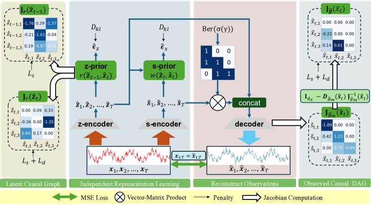
Figure 3: The estimation procedure of NCDL. The model framework includes two encoders: z-encoder for extracting latent variables $\mathbf{z}_{t}$, and s-encoder for extracting $\mathbf{s}_{t}$. A decoder reconstructs observations from these variables. Additionally, prior networks estimate the prior distribution using normalizing flow, target on learning causal structure based on Jacobian matrix. $L_{s}$ imposes a sparsity constraint and $L_{d}$ enforces the DAG structure on Jacobian matrix. $D_{kl}$ enforces an independence constraint on the estimated noise by minimizing its KL divergence w.r.t. $\mathcal{N}(0,\mathbf{I})$.

Overall architecture.

According to the data generation process 2.2, we establish the Evidence Lower BOund (ELBO) as follows:

$$\mathcal{L}_{ELBO}=\mathbb{E}_{q(\mathbf{s}_{1:T}\mid\mathbf{x}_{1:T})}\left[\log p(\mathbf{x}_{1:T}\mid\mathbf{s}_{1:T},\mathbf{z}_{1:T})\right]-\lambda_{1}D_{kl}(q(\mathbf{s}_{1:T}\mid\mathbf{x}_{1:T})\|p(\mathbf{s}_{1:T}\mid\mathbf{z}_{1:T}))$$ (10)

$$-\lambda_{2}D_{kl}(q(\mathbf{z}_{1:T}\mid\mathbf{x}_{1:T})\|p(\mathbf{z}_{1:T})),$$

Where $\lambda_{1}$ and $\lambda_{2}$ are hyperparameters, and $D_{kl}$ represents the Kullback-Leibler divergence. We set $\lambda_{1}=4\times 10^{-3}$ and $\lambda_{2}=1.0\times 10^{-2}$ to achieve the best performance. In Figure 3, the z-encoder, s-encoder and decoder implemented by Multi-Layer Perceptrons (MLPs) are defined as:

respectively, where the neural network $\phi$, z-encoder learns the latent variables through denoising, and s-encoder $\psi$ and decoder $\eta$ approximate invertible functions for encoding and reconstruction of nonlinear ICA, respectively.

Prior estimation of $\mathbf{z}_{t}$ and $\mathbf{s}_{t}$.

We propose using the s-prior network and z-prior network to recover the independent noise $\hat{\bm{\epsilon}}_{x_{t}}$ and $\hat{\bm{\epsilon}}_{z_{t}}$, respectively, thereby estimating the prior distribution of latent variables $\hat{\mathbf{z}}_{t}$ and dependent noise $\hat{\mathbf{s}}_{t}$. Specifically, we first let ${r_{i}}$ be the $i$-th learned inverse transition function that take the estimated latent variables as input to recover the noise term, e.g., $\hat{\epsilon}_{z_{t,i}}=r_{i}(\hat{{\mathbf{z}}}_{t-1},\hat{{\mathbf{z}}}_{t})$. Each $r_{i}$ is implemented by MLPs. Sequentially, we devise a transformation $\kappa:=\{\hat{{\mathbf{z}}}_{t-1},\hat{{\mathbf{z}}}_{t}\}\rightarrow\{\hat{{\mathbf{z}}}_{t-1},\hat{\bm{\epsilon}}_{z_{t}}\}$, whose Jacobian can be formalized as ${\mathbf{J}_{\kappa}=\begin{pmatrix}\mathbf{I}&0\\ \mathbf{J}_{r}(\hat{\mathbf{z}}_{t-1})&\mathbf{J}_{r}(\hat{\mathbf{z}}_{t})\end{pmatrix}}$. Then we have Eq. 11 derived from normalizing flow (Rezende & Mohamed, 2015).

$$\log p(\hat{{\mathbf{z}}}_{t},\hat{{\mathbf{z}}}_{t-1})=\log p(\hat{{\mathbf{z}}}_{t-1},\hat{\bm{\epsilon}}_{z_{t}})+\log|\frac{\partial r_{i}}{\partial\hat{z}_{t,i}}|.$$ (11)

According to the generation process, the noise $\epsilon_{z_{t,i}}$ is independent of ${\mathbf{z}}_{t-1}$, allowing us to enforce independence on the estimated noise term $\hat{\epsilon}_{z_{t,i}}$ with $\mathcal{L}_{kl}$. Consequently, Eq. 11 can be rewritten as:

$$\log p(\hat{{\mathbf{z}}}_{1:T})=p(\hat{{\mathbf{z}}}_{1})\prod_{\tau=2}^{T}\left(\sum_{i=1}^{d_{z}}\log p(\hat{\epsilon}_{z_{\tau,i}})+\sum_{i=1}^{d_{z}}\log|\frac{\partial r_{i}}{\partial\hat{z}_{\tau,i}}|\right),$$ (12)

where $p(\hat{\epsilon}_{z_{\tau,i}})$ is assumed to follow a Gaussian distribution. Similarly, we estimate the prior of $\mathbf{s}_{t}$ using $\hat{\epsilon}_{x_{t,i}}=w_{i}(\hat{{\mathbf{z}}}_{t},\hat{{\mathbf{s}}}_{t})$, and model the transformation between $\hat{\mathbf{s}}_{t}$ and $\hat{\mathbf{z}}_{t}$ as follows:

$$\log p\left(\hat{\mathbf{s}}_{1:T}\mid\hat{\mathbf{z}}_{1:T}\right)=\prod_{\tau=1}^{T}\left(\sum_{i=1}^{d_{x}}\log p\left(\hat{\epsilon}_{x_{\tau,i}}\right)+\sum_{i=1}^{d_{x}}\log\left|\frac{\partial w_{i}}{\partial\hat{s}_{\tau,i}}\right|\right).$$ (13)

Specifically, to ensure the conditional independence of $\hat{\mathbf{z}}_{t}$ and $\hat{\mathbf{s}}_{t}$, we using $\mathcal{L}_{kl}$ to minimize the KL divergence from the distributions of $\hat{\bm{\epsilon}}_{x_{t}}$ and $\hat{\bm{\epsilon}}_{z_{t}}$ to the distribution $\mathcal{N}(0,\mathbf{I})$.

Structure learning.

The variables $r_{i}$ and $w_{i}$ are designed to capture causal dependencies among latent and observed variables, respectively. We denote $\mathbf{J}_{r}(\hat{\mathbf{z}}_{t-1})$ as the Jacobian matrix of the function $r$, which implies the estimated time-lagged latent causal structure; $\mathbf{J}_{r}(\hat{\mathbf{z}}_{t})$, which implies the estimation of instantaneous latent causal structure; and $\mathbf{J}_{\hat{g}}(\hat{\mathbf{x}}_{t})$, which implies the estimated observed causal DAG. Considering the observed causal DAG, we first obtain the basic structure of the observed causal DAG by learning a binary mask $\mathcal{M}\sim\operatorname{Ber}(\sigma(\gamma))$, where each edge $\mathcal{M}_{i,j}$ is an independent Bernoulli random variable with parameter $\sigma(\gamma_{i,j})$. The Gumbel-Softmax technique is employed to learn $\gamma$ (Jang et al., 2017; Maddison et al., 2017), following Ng et al. (2022). Subsequently, we obtained $\mathbf{J}_{\hat{g}_{m}}(\hat{\mathbf{s}}_{t})$ from the decoder, and compute the observed causal DAG $\mathbf{J}_{\hat{g}}(\hat{\mathbf{x}}_{t})$ via Corollary. 3.6. Notably, the entries of $\mathbf{J}_{\hat{g}}(\hat{\mathbf{x}}_{t})$ vary with other variables such as $\hat{\mathbf{z}}_{t}$, resulting in a DAG that could change over time. For the latent structure, we directly compute $\mathbf{J}_{r}(\hat{\mathbf{z}}_{t-1})$ and $\mathbf{J}_{r}(\hat{\mathbf{z}}_{t})$ from z-prior network as the time-lagged structure and instantaneous DAG in latent space, respectively. To prevent redundant edges and cycles, a sparsity penalty $\mathcal{L}_{s}$ are imposed on each learned structure, and DAG constraint $\mathcal{L}_{d}$ are imposed on observed causal DAG and instantaneous latent causal DAG. Specifically, the Markov network structure for latent variables is derived as the off-diagonal matrix of $\mathcal{M}(\mathbf{J})=(\mathbf{I}+\mathbf{J})^{\top}(\mathbf{I}+\mathbf{J})$. Formally, we define the penalties as follows:

$$\sum\mathcal{L}_{s}=||\mathcal{M}(\mathbf{J}_{r}(\hat{\mathbf{z}}_{t}))||_{1}+||\mathcal{M}(\mathbf{J}_{r}(\hat{\mathbf{z}}_{t-1}))||_{1}+||\mathbf{J}_{\hat{g}}(\hat{\mathbf{x}}_{t})||_{1};\quad\sum\mathcal{L}_{d}=\mathcal{D}(\mathbf{J}_{\hat{g}}(\hat{\mathbf{x}}_{t}))+\mathcal{D}(\mathbf{J}_{r}(\hat{\mathbf{z}}_{t})),$$ (14)

where $\mathcal{D}(A)=\operatorname{tr}\left[(I+\frac{1}{m}A\circ A)^{m}\right]-m$ is the DAG constraint from (Yu et al., 2019), with $A$ being an $m$-dimensional matrix. $||\cdot||_{1}$ denotes the matrix $l_{1}$ norm. In summary, the overall loss function of the NCDL model is formalized as:

$$\mathcal{L}_{all}=\mathcal{L}_{ELBO}+\alpha\sum\mathcal{L}_{s}+\beta\sum\mathcal{L}_{d},$$ (15)

where $\alpha=1.0\times 10^{-4}$ and $\beta=5.0\times 10^{-5}$ are hyperparameters. The discussion on selecting hyperparameter is given in Appendix C.1.

5 Experiment

5.1 Synthetic Data

Empirical study.

The evaluation metrics and their connections to our theorems is elaborated in Appendix C.1. We show performance on of the general nonlinear causal discovery and representation learning in Table 1, and investigate different dimensionalities of observed variables, including $d_{x}=\{3,6,8,10,100^{*}\}$ (* means add mask by simulated inductive bias, see detailed Appendix C.1). Our results on these metrics verify the effectiveness of our methodology under identifiabilty, and the result on $d_{x}=100$ with inductive bias makes it scalable to high-dimensional data with prior knowledge of the elimination of some dependences provided by the physical law of climate (Ebert-Uphoff & Deng, 2012) or LLM (Long et al., 2023), supports our subsequent experiment on real-world data. The study on different $d_{z}$ can be found in Appendix C.1. Additionally, verification of our theoretical assumptions through an ablation study can be found in Appendix C.1.

$d_{z}$	$d_{x}$	SHD ($\mathbf{J}_{\hat{g}}(\hat{\mathbf{x}}_{t})$)	TPR	Precision	MCC ($\mathbf{s}_{t}$)	MCC ($\mathbf{z}_{t}$)	SHD ($\mathbf{J}_{r}(\hat{\mathbf{z}}_{t})$)	SHD ($\mathbf{J}_{r}(\hat{\mathbf{z}}_{t-1})$)	$R^{2}$
3	3	0	1	1	0.9775 ($\pm$0.01)	0.9721 ($\pm$0.01)	0.27 ($\pm$0.05)	0.26 ($\pm$0.03)	0.90 ($\pm$0.05)
	6	0.18 ($\pm$0.06)	0.83 ($\pm$0.03)	0.80 ($\pm$0.04)	0.9583 ($\pm$0.02)	0.9505 ($\pm$0.01)	0.24 ($\pm$0.06)	0.33 ($\pm$0.09)	0.92 ($\pm$0.01)
	8	0.29 ($\pm$0.05)	0.78 ($\pm$0.05)	0.76 ($\pm$0.04)	0.9020 ($\pm$0.03)	0.9601 ($\pm$0.03)	0.36 ($\pm$0.11)	0.31 ($\pm$0.12)	0.93 ($\pm$0.02)
	10	0.43 ($\pm$0.05)	0.65 ($\pm$0.08)	0.63 ($\pm$0.14)	0.8504 ($\pm$0.07)	0.9652 ($\pm$0.02)	0.29 ($\pm$0.04)	0.40 ($\pm$0.05)	0.92 ($\pm$0.02)
	100∗	0.17 ($\pm$0.02)	0.80 ($\pm$0.05)	0.81 ($\pm$0.02)	0.9131 ($\pm$0.02)	0.9565 ($\pm$0.02)	0.21 ($\pm$0.01)	0.29 ($\pm$0.10)	0.93 ($\pm$0.03)

Table 1: Results on different observed dimensionality $d_{x}$. We run simulations with 5 random seeds, selected based on the best-converged results to avoid local minima.

Comparison with constraint-based methods on observed causal DAG.

To the best of our knowledge, no existing method employs a comparably general framework based on structural equation models. Therefore, we compare our approach against two constraint-based methods: FCI (Spantini et al., 2018) and CD-NOD (Huang et al., 2020), both of which are designed to discover causal DAGs while accounting for latent confounders. Additionally, we evaluate methods proposed for causal discovery on time-series data, including PCMCI (Runge et al., 2019), a climate-specific method that incorporates time-lagged and instantaneous effects, as well as LPCMCI (Gerhardus & Runge, 2020), which is proposed for causal discovery in observational time series in the presence of latent confounders and autocorrelation. As illustrated in Fig.4, NCDL demonstrates superior performance across different sample sizes, with further improvements observed as the sample size increases. We observe that FCI struggles when latent confounders are dependent on each other, often resulting in low recall. CD-NOD assumes pseudo-causal sufficiency, requiring latent confounders to be functions of surrogate variables, which is incompatible with general latent variable settings. PCMCI ignores latent variables and underlying processes, while LPCMCI, despite considering latent variables, cannot handle latent processes and requires the absence of edges among latent confounders. These constraints collectively highlight the advantages of our approach in addressing such challenges. Additional experimental details can be found in AppendixC.1.

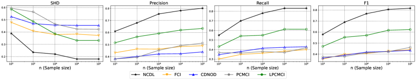
Figure 4: Comparison with constraint-based methods. We set $d_{x}=6$ and $d_{z}=3$. We run experiments using 5 different random seeds, and report the average performance on evaluation metrics.

Comparison with temporal (causal) representation learning.

We evaluate our method against the following compared methods including CaRiNG (Chen et al., 2024), TDRL (Yao et al., 2022), LEAP (Yao et al., 2021), SlowVAE (Klindt et al., 2020), PCL (Hyvarinen & Morioka, 2017), i-VAE (Khemakhem et al., 2020), TCL (Hyvarinen & Morioka, 2016), and methods handling instantaneous dependencies including iCITRIS (Lippe et al., 2022) and G-CaRL (Morioka & Hyvärinen, 2023) in Table 2. The dimensions are set to $d_{z}=3$ and $d_{x}=10$. The MCC and $R^{2}$ results for the Independent and Sparse settings demonstrate that our model achieves component-wise identifiability (Theorem 3.3). In contrast, other considered methods fail to recover latent variables, as they cannot properly address cases where the observed variables are causally-related. For the Dense setting, our approach achieves monoblock identifiability (Theorem 3.2) with the highest $R^{2}$, while other methods exhibit significant degradation because they are not specifically tailored to handle scenarios involving general noise in the generating function. These outcomes are consistent with our theoretical analysis.

Setting	Metric	NCDL	iCITRIS	G-CaRL	CaRiNG	TDRL	LEAP	SlowVAE	PCL	i-VAE	TCL
Independent	MCC	0.9811	0.6649	0.8023	0.8543	0.9106	0.8942	0.4312	0.6507	0.6738	0.5916
	$R^{2}$	0.9626	0.7341	0.9012	0.8355	0.8649	0.7795	0.4270	0.4528	0.5917	0.3516
Sparse	MCC	0.9306	0.4531	0.7701	0.4924	0.6628	0.6453	0.3675	0.5275	0.4561	0.2629
	$R^{2}$	0.9102	0.6326	0.5443	0.2897	0.6953	0.4637	0.2781	0.1852	0.2119	0.3028
Dense	MCC	0.6750	0.3274	0.6714	0.4893	0.3547	0.5842	0.1196	0.3865	0.2647	0.1324
	$R^{2}$	0.9204	0.6875	0.8032	0.4925	0.7809	0.7723	0.5485	0.6302	0.1525	0.206

Table 2: Experiments results on simulated data. We consider three scenarios according to our theory: Independent: $z_{t,i}$ and $z_{t,j}$ are conditionally independent given $\mathbf{z}_{t-1}$; Sparse: $z_{t,i}$ and $z_{t,j}$ are dependent given $\mathbf{z}_{t-1}$, but the latent Markov network $\mathcal{G}_{z_{t}}$ and time-lagged latent structure are sparse; Dense: No sparsity restrictions on latent causal graph. Bold numbers indicate the best performance.

5.2 Real-world Data

We use the CESM2 sea surface temperature dataset as our real-world data source for temperature forecasting and causal structure learning. Due to page limitations, implementation details are provided in Appendix C.2. Our analysis yields two main results: i) temperature forecasting, which demonstrates the effectiveness of the learned representations, and ii) visualization of the inferred causal graph across regions, validated against contemporaneous wind patterns. As summarized in Table 3, our approach surpasses existing time-series forecasting models in precision, due to existing temporal causal representation learning cannot handle cases where observations are causally-related and the generating function is non-invertible, restricting their usability in real-world climate data. Computational cost of NCDL with other methods in the experiments can be seen in paragraph. 7. To compare against the estimated observed causal DAG, we use wind data from (Rasp et al., 2020) for the same period. In Fig. 5, the inferred causal structures closely correspond to actual wind patterns over the sea surface, accurately capturing the overall spatial dynamics and corroborating prior findings. Moreover, regions near coastlines exhibit denser causal connections, suggesting potential influences from anthropogenic activities or topographic features, thereby enriching our understanding of the underlying mechanisms governing the climate system.

		NCDL (Ours)		TDRL		CARD		FITS		MICN		iTransformer		TimesNet		Autoformer
Dataset	Len	MSE	MAE	MSE	MAE	MSE	MAE	MSE	MAE	MSE	MAE	MSE	MAE	MSE	MAE	MSE	MAE
CESM2	96	0.410	0.483	0.439	0.507	0.409	0.484	0.439	0.508	0.417	0.486	0.422	0.491	0.415	0.486	0.959	0.735
CESM2	192	0.412	0.487	0.440	0.508	0.422	0.493	0.447	0.515	1.559	0.984	0.425	0.495	0.417	0.497	1.574	0.972
CESM2	336	0.413	0.485	0.441	0.505	0.421	0.497	0.482	0.536	2.091	1.173	0.426	0.494	0.423	0.499	1.845	1.078

Table 3: The MSE and MAE results for different prediction lengths in temperature forecasting. Lower values indicate better forecasting performance. Bold numbers represent the best performance among the models, while underlined numbers denote the second-best performance.

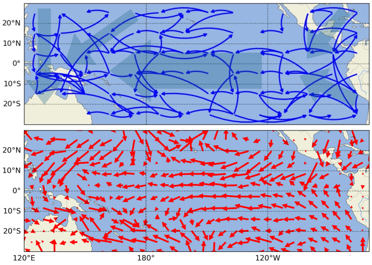
Figure 5: Comparison of observed causal DAG obtained by NCDL and wind system. Top: Visualization of learned instantaneous causal graph. Bottom: Visualization of the wind system. The blue arrows indicate the causal adjacency, while the red arrows represent the wind direction in the respective area. Notably, NCDL effectively identifies the underlying causal graph, showing a high degree of overlap with the real-world system. For instance, it captures the westward trend in the central sea region. However, in the sea/land interaction zones, the learned causal edges appear disorganized, losing clear patterns and becoming much denser than in other regions. Our result suggests that causal relationships are more intricate in these areas beyond wind system, likely due to the influence of human activities Vautard et al. (2019) and other factors arising from soil-atmosphere/cloud-temperature interactions, and land–sea warming contrasts Boé & Terray (2014).

6 Conclusion

We establish identifiability results for uncovering latent causal variables, latent Markov network, and observed causal DAG, especially in complex nonlinear systems such as climate science. Simulated experiments validate our theoretical findings, and real-world experiments offer causal insights for climate science.

For future work, we aim to address the issue of performance degradation in data with increasing dimensionality. A possible approach to tackling this challenge is to resort to the divide-and-conquer strategy, which partitions the high-dimensional problem into a set of overlapping subsets of variables with lower dimensionality, leveraging the prior knowledge of geographical information.

Supplement to
 
“Identification of Nonparametric Dynamic Causal Model and Latent Process for Climate Analysis”

Appendix A Theorem Proofs

A.1 Notation List

Index	Explanation	Value
$d_{x}$	number of observed variables	$d_{x}\in\mathbb{N}^{+}$
$d_{z}$	number of latent variables	$d_{z}\in\mathbb{N}^{+}$ and $d_{z}\leq d_{x}$
$t$	time index	$t\in\mathbb{N}^{+}$ and $t\geq 3$
$\mathcal{I}$	index set of observed variables	$\mathcal{I}=\{1,2,\ldots,d_{x}\}$
$\mathcal{J}$	index set of latent variables	$\mathcal{J}=\{1,2,\ldots,d_{z}\}$
Variable	Explanation	Value
$\mathcal{X}_{t}$	support of observed variables in time-index $t$	$\mathcal{X}_{t}\subseteq\mathbb{R}^{d_{x}}$
$\mathcal{Z}_{t}$	support of latent variables	$\mathcal{Z}_{t}\subseteq\mathbb{R}^{d_{z}}$
$\mathbf{x}_{t}$	observed variables in time-index $t$	$\mathbf{x}_{t}\in\mathcal{X}_{t}$
$\mathbf{z}_{t}$	latent variables in time-index $t$	$\mathbf{z}_{t}\in\mathcal{Z}_{t}$
$\mathbf{s}_{t}$	dependent noise of observations in time-index $t$	$\mathbf{s}_{t}\in\mathbb{R}^{d_{x}}$
$\bm{\epsilon}_{\mathbf{x}_{t}}$	independent noise for generating $\mathbf{s}_{t}$ in time-index $t$	$\bm{\epsilon}_{\mathbf{x}_{t}}\sim p_{\epsilon_{x}}$
$\bm{\epsilon}_{\mathbf{z}_{t}}$	independent noise of latent variables in time-index $t$	$\bm{\epsilon}_{\mathbf{z}_{t}}\sim p_{\epsilon_{z}}$
$\mathbf{z}_{t\setminus[i,j]}$	latent variables except for $z_{t,i}$ and $z_{t,j}$ in time-index $t$	/
Function	Explanation	Value
$p_{a}(\cdot\mid b)$	density function of $a$ given $b$	/
$p_{b}(a,\cdot\mid c)$	joint density function of $(a,b)$ given $a$ and $c$	/
$\mathbf{pa}(\cdot)$	variable’s parents	/
$\mathbf{pa}_{O}(\cdot)$	variable’s parents in observed space	/
$\mathbf{pa}_{L}(\cdot)$	variable’s parents in latent space	/
$\mathbf{an}_{L}(\cdot)$	variable’s ancestors in $\mathbf{z}_{t}$	/
$g(\cdot)$	generating function of SEM from $(\mathbf{z}_{t},\mathbf{s}_{t},\mathbf{x}_{t})$ to $\mathbf{x}_{t}$	$\mathbb{R}^{d_{z}+2d_{x}}\rightarrow\mathbb{R}^{d_{x}}$
$g_{m}(\cdot)$	mixing function of ICA from $(\mathbf{z}_{t},\mathbf{s}_{t})$ to $\mathbf{x}_{t}$	$\mathbb{R}^{d_{z}+d_{x}}\rightarrow\mathbb{R}^{d_{x}}$
$h_{z}(\cdot)$	invertible transformation from $\mathbf{z}_{t}$ to $\hat{\mathbf{z}}_{t}$	$\mathbb{R}^{d_{z}}\rightarrow\mathbb{R}^{d_{z}}$
$\pi(\cdot)$	permutation function	$\mathbb{R}^{d_{x}}\rightarrow\mathbb{R}^{d_{x}}$
$\text{supp}(\cdot)$	support matrix of Jacobian matrix	$\mathbb{R}^{d_{x}\times d_{x}}\rightarrow\{0,1\}^{d_{x}\times d_{x}}$
Symbol	Explanation	Value
$\mathcal{G}_{\mathbf{x}_{t}}$	causal graph among observed variables (observed causal DAG) in $t$	/
$\mathcal{G}_{\mathbf{z}_{t}}$	causal graph among latent variables in time-index $t$	/
$A\rightarrow B$	$A$ causes $B$ directly	/
$A\dashrightarrow B$	$A$ causes $B$ indirectly	/
$\mathbf{J}_{g}(\mathbf{x}_{t})$	Jacobian matrix representing observed causal DAG	$\mathbf{J}_{g}(\mathbf{x}_{t})\in\mathbb{R}^{d_{x}\times d_{x}}$
$\mathbf{J}_{g}(\mathbf{x}_{t},\mathbf{s}_{t})$	Jacobian matrix representing mixing structure from $(\mathbf{x}_{t},\mathbf{s}_{t})$ to $\mathbf{x}_{t}$	$\mathbf{J}_{g}(\mathbf{x}_{t},\mathbf{s}_{t})\in\mathbb{R}^{d_{x}\times d_{x}}$
$\mathbf{J}_{g_{m}}(\mathbf{s}_{t})$	Jacobian matrix representing mixing structure from $\mathbf{s}_{t}$ to $\mathbf{x}_{t}$	$\mathbf{J}_{g_{m}}(\mathbf{s}_{t})\in\mathbb{R}^{d_{x}\times d_{x}}$
$\mathbf{J}_{r}(\mathbf{z}_{t-1})$	Jacobian matrix representing latent time-lagged structure	$\mathbf{J}_{r}(\mathbf{z}_{t-1})\in\mathbb{R}^{d_{z}\times d_{z}}$
$\mathbf{J}_{r}(\mathbf{z}_{t})$	Jacobian matrix representing instantaneous latent causal graph	$\mathbf{J}_{r}(\mathbf{z}_{t})\in\mathbb{R}^{d_{z}\times d_{z}}$

Table 4: List of notations, explanations and corresponding values.

A.2 Proof of Theorem 3.2

Outline.

This proof builds on the strategy employed in nonparametric identification methods within econometrics Hu & Schennach (2008); Hu & Shum (2012), but differs in its underlying assumptions and final results. We begin by utilizing the properties of our model to derive a spectral decomposition form. Next, the uniqueness of this decomposition is established by referencing the spectral decomposition theorem for bounded linear operators provided in Hu & Schennach (2008); Dunford & Schwartz (1988). Finally, we address certain indeterminacy arising from the decomposition process and demonstrate how they can be resolved, culminating in our main results. Preliminaries are shown as follows for the readability.

A.2.1 Preliminary

Definition A.1

(Diagonal Operator) Consider two random variable $a$ and $b$, density functions $p_{a}$ and $p_{b}$ are defined on some support $\mathcal{A}$ and $\mathcal{B}$, respectively. The diagonal operator $D_{b\mid a}$ maps the density function $p_{a}$ to another density function $D_{b\mid a}\circ p_{a}$ defined by the pointwise multiplication of the function $p_{b\mid a}$ at a fixed point $b$:

$$\mathcal{F}(\mathcal{A})\rightarrow\mathcal{F}(\mathcal{B}):\quad D_{b\mid a}\circ p_{a}=p_{b\mid a}(b\mid\cdot)p_{a}.$$ (16)

Definition A.2

(Permuting Operator) Consider two random variable $a$ and $b$, density functions $p_{a}$ and $p_{b}$ are defined on some support $\mathcal{A}$ and $\mathcal{B}$, respectively, where $\mathcal{A}=\mathcal{B}$. The permutation operator $P_{b\mid a}$ maps the density function $p_{a}$ to another density function $p_{b}$, which is defined by the pointwise permutation of each density of $p_{a}$ at a point $a$:

$$\mathcal{F}(\mathcal{A})\rightarrow\mathcal{F}(\mathcal{B}):\quad p_{b}=P_{b\mid a}\circ p_{a}=p_{a}(g(\cdot)),\quad b=g(a),$$ (17)

where $g$ is an invertible function.

Definition A.3

(Completeness) A family of conditional density function $p(a|b)$ is complete if the only solution $p(a)$ to

$$\int_{A}p(a)p_{a|b}(a|b)\,da=0\quad\forall b\in\mathcal{B}$$ (18)

is $p(a)=0$. In other words, no matter the range of an operator is on finite or infinite, it is complete if its null space or kernel is a zero set. Completeness is always used to phrase the sufficient and necessary condition for injective linear operator (Newey & Powell, 2003; Chernozhukov et al., 2007).

Properties of linear operator.

We outline useful properties of the linear operator to facilitate understanding of our proof:

1. (Inverse) If linear operator: $L_{b\mid a}$ exists a left-inverse $L_{b\mid a}^{-1}$, such $L_{b\mid a}^{-1}\circ L_{b\mid a}\circ p_{a}=p_{a}$ for all $a\in\mathcal{A}$. Analogously, if $L_{b\mid a}$ exists a right-inverse $L_{b\mid a}^{-1}$, such $L_{b\mid a}\circ L_{b\mid a}^{-1}\circ p_{a}=p_{a}$ for all $a\in\mathcal{A}$. If $L_{b\mid a}$ is bijective, there exists left-inverse and right-inverse which are the same.

2. (Injective) $L_{b|a}$ is said to be an injective linear operator if its $L^{-1}_{b|a}$ is defined over the range of the operator $L_{b|a}$ (Kress et al., 1989). If so, under assumption a), $L_{a|b}^{-1}$ exists and is densely defined over $\mathcal{F}(\mathcal{A})$. (Hu & Schennach, 2008).

3. (Composition) Given two linear operators $L_{c\mid b}:\mathcal{F}(\mathcal{B})\rightarrow\mathcal{F}(\mathcal{C})$ and $L_{c\mid a}:\mathcal{F}(\mathcal{A})\rightarrow\mathcal{F}(\mathcal{C})$, with the function space supports defined uniformly on the range of supports for the domain spaces as characterized by $L_{b\mid a}$, it follows that $L_{c\mid a}=L_{c\mid b}\circ L_{b\mid a}$. Furthermore, the properties of linearity and associativity are preserved in the operation of linear operators. However, it is crucial to note the non-commutativity of these operators, i.e., $L_{c\mid b}L_{b\mid a}\neq L_{b\mid a}L_{c\mid b}$, indicating the significance of the order of application.

A.2.2 Detailed Proof

Step I: implications of conditional independence.

The definition of latent causal process indicates that $\mathbf{x}_{t-1},\mathbf{x}_{t},\mathbf{x}_{t+1}$ are conditional independent given $\mathbf{z}_{t}$, which implies two equations:

• $p(\mathbf{x}_{t-1}\mid\mathbf{x}_{t},\mathbf{z}_{t})=p(\mathbf{x}_{t-1}\mid\mathbf{z}_{t})$

• $p(\mathbf{x}_{t+1}\mid\mathbf{x}_{t},\mathbf{x}_{t-1},\mathbf{z}_{t})=p(\mathbf{x}_{t+1}\mid\mathbf{z}_{t}).$

Step II: transformation in function space.

The observed $p(\mathbf{x}_{t-1})$ and joint distribution $p(\mathbf{x}_{t+1},\mathbf{x}_{t},\mathbf{x}_{t-1})$ directly indicates $p(\mathbf{x}_{t+1},\mathbf{x}_{t}\mid\mathbf{x}_{t-1})$, and then the processes of motions are established by noting that

$$p(\mathbf{x}_{t+1},\mathbf{x}_{t}\mid\mathbf{x}_{t-1}) =\int_{\mathcal{Z}_{t}}p(\mathbf{x}_{t+1},\mathbf{x}_{t},\mathbf{z}_{t}\mid\mathbf{x}_{t-1})d\mathbf{z}_{t}$$ (19)

$$=\int_{\mathcal{Z}_{t}}p(\mathbf{x}_{t+1}\mid\mathbf{x}_{t},\mathbf{z}_{t},\mathbf{x}_{t-1})p(\mathbf{x}_{t},\mathbf{z}_{t}\mid\mathbf{x}_{t-1})d\mathbf{z}_{t}$$

$$=\int_{\mathcal{Z}_{t}}p(\mathbf{x}_{t+1}\mid\mathbf{z}_{t})p(\mathbf{x}_{t},\mathbf{z}_{t}\mid\mathbf{x}_{t-1})d\mathbf{z}_{t}$$

$$=\int_{\mathcal{Z}_{t}}p(\mathbf{x}_{t+1}\mid\mathbf{z}_{t})p(\mathbf{x}_{t}\mid\mathbf{z}_{t},\mathbf{x}_{t-1})p(\mathbf{z}_{t}\mid\mathbf{x}_{t-1})d\mathbf{z}_{t}$$

$$=\int_{\mathcal{Z}_{t}}p(\mathbf{x}_{t+1}\mid\mathbf{z}_{t})p(\mathbf{x}_{t}\mid\mathbf{z}_{t})p(\mathbf{z}_{t}\mid\mathbf{x}_{t-1})d\mathbf{z}_{t}.$$

We incorporate the integration over $\mathcal{X}_{t-1}$,

$$\int_{\mathcal{X}_{t-1}}p(\mathbf{x}_{t+1},\mathbf{x}_{t}\mid\mathbf{x}_{t-1})p(\mathbf{x}_{t-1})d\mathbf{x}_{t-1}=\int_{\mathcal{X}_{t-1}}\int_{\mathcal{Z}_{t}}p(\mathbf{x}_{t+1}\mid\mathbf{z}_{t})p(\mathbf{x}_{t}\mid\mathbf{z}_{t})p(\mathbf{z}_{t}\mid\mathbf{x}_{t-1})p(\mathbf{x}_{t-1})d\mathbf{z}_{t}d\mathbf{x}_{t-1}$$ (20)

Step III: construct spectral decomposition.

By the definition of linear operator 3.1,

$$\int_{\mathcal{X}_{t-1}}p(\mathbf{x}_{t+1},\mathbf{x}_{t}\mid\mathbf{x}_{t-1})p(\mathbf{x}_{t-1})d\mathbf{x}_{t-1}=[L_{\mathbf{x}_{t};\mathbf{x}_{t+1}\mid\mathbf{x}_{t-1}}\circ p](\mathbf{x}_{t-1}),$$ (21)

where $L_{\mathbf{x}_{t};\mathbf{x}_{t+1}\mid\mathbf{x}_{t-1}}=\int_{\mathcal{X}_{t-1}}p_{\mathbf{x}_{t+1}}(\mathbf{x}_{t},\cdot\mid\mathbf{x}_{t-1})p(\mathbf{x}_{t-1})d{\mathbf{x}_{t-1}}$. Through the definition of diagonal operator A.1, we have

$$[L_{\mathbf{x}_{t};\mathbf{x}_{t+1}\mid\mathbf{x}_{t-1}}p](\mathbf{x}_{t+1})=[L_{{\mathbf{x}_{t+1}\mid\mathbf{z}_{t}}}D_{{\mathbf{x}_{t}\mid\mathbf{z}_{t}}}L_{\mathbf{z}_{t}\mid\mathbf{x}_{t-1}}p](\mathbf{x}_{t-1}),$$ (22)

which implies the operator equivalence:

$$L_{\mathbf{x}_{t};\mathbf{x}_{t+1}\mid\mathbf{x}_{t-1}}=L_{{\mathbf{x}_{t+1}\mid\mathbf{z}_{t}}}D_{\mathbf{x}_{t}\mid\mathbf{z}_{t}}L_{\mathbf{z}_{t}\mid\mathbf{x}_{t-1}}.$$ (23)

Let’s integrating out $\mathbf{x}_{t}$. First,

$$\int_{\mathbf{x}_{t}\in\mathcal{X}_{t}}L_{\mathbf{x}_{t};\mathbf{x}_{t+1}\mid\mathbf{x}_{t-1}}\,d\mathbf{x}_{t}=\int_{\mathbf{x}_{t}\in\mathcal{X}_{t}}L_{{\mathbf{x}_{t+1}\mid\mathbf{z}_{t}}}D_{\mathbf{x}_{t}\mid\mathbf{z}_{t}}L_{\mathbf{z}_{t}\mid\mathbf{x}_{t-1}}\,d\mathbf{x}_{t}$$

then we get

$$L_{\mathbf{x}_{t+1}\mid\mathbf{x}_{t-1}}=L_{\mathbf{x}_{t+1}\mid\mathbf{z}_{t}}L_{\mathbf{z}_{t}\mid\mathbf{x}_{t-1}}.$$ (24)

In Assumption b), the linear operator $L_{\mathbf{x}_{t+1}\mid\mathbf{z}_{t}}$ is injective, Eq. 24 can be written as

$$L^{-1}_{\mathbf{x}_{t+1}\mid\mathbf{z}_{t}}L_{\mathbf{x}_{t+1}\mid\mathbf{x}_{t-1}}=L_{\mathbf{z}_{t}\mid\mathbf{x}_{t-1}}.$$ (25)

The $L_{{\mathbf{z}_{t}\mid\mathbf{x}_{t-1}}}$ in Eq. 23 could be substituted by Eq. 25:

$$L_{\mathbf{x}_{t};\mathbf{x}_{t+1}\mid\mathbf{x}_{t-1}}=L_{{\mathbf{x}_{t+1}\mid\mathbf{z}_{t}}}D_{\mathbf{x}_{t}\mid\mathbf{z}_{t}}L^{-1}_{\mathbf{x}_{t+1}\mid\mathbf{z}_{t}}L_{\mathbf{x}_{t+1}\mid\mathbf{x}_{t-1}}.$$ (26)

According to Lemma 1 in (Hu & Schennach, 2008), if $L_{\mathbf{x}_{t-1}\mid\mathbf{x}_{t+1}}$ is injective, then $L^{-1}_{\mathbf{x}_{t+1}\mid\mathbf{x}_{t-1}}$ exists and is densely defined over $f(\mathcal{X}_{t+1})$, we have

$$L_{\mathbf{x}_{t};\mathbf{x}_{t+1}\mid\mathbf{x}_{t-1}}L^{-1}_{\mathbf{x}_{t+1}\mid\mathbf{x}_{t-1}}=L_{\mathbf{x}_{t+1}\mid\mathbf{z}_{t}}D_{\mathbf{x}_{t}\mid\mathbf{z}_{t}}L^{-1}_{\mathbf{x}_{t+1}\mid\mathbf{z}_{t}}.$$ (27)

Step IV: uniqueness of spectral decomposition

Obviously, $L_{\mathbf{x}_{t};\mathbf{x}_{t+1}\mid\mathbf{x}_{t-1}}L^{-1}_{\mathbf{x}_{t+1}\mid\mathbf{x}_{t-1}}$ is a spectral decomposition form. By Assumption b), the linear operator is bounded. Consequently, $L_{\mathbf{x}_{t};\mathbf{x}_{t+1}\mid\mathbf{x}_{t-1}}L^{-1}_{\mathbf{x}_{t+1}\mid\mathbf{x}_{t-1}}$ is also bounded, which is fit the requirements in  (Hu & Schennach, 2008). As established in Section XV.4 of Dunford & Schwartz (1988), which capply Theorem XV.4.3.5 in (Dunford & Schwartz, 1988) to demonstrate that the spectral decomposition of $L_{\mathbf{x}_{t};\mathbf{x}_{t+1}\mid\mathbf{x}_{t-1}}L^{-1}_{\mathbf{x}_{t+1},\mathbf{x}_{t-1}}$ is unique, and also, $L_{\mathbf{x}_{t};\mathbf{x}_{t+1}\mid\mathbf{x}_{t-1}}L^{-1}_{\mathbf{x}_{t+1},\mathbf{x}_{t-1}}$ is observed, thus the operator $L_{\mathbf{x}_{t+1}\mid\mathbf{z}_{t}}D_{\mathbf{x}_{t}\mid\mathbf{z}_{t}}L^{-1}_{\mathbf{x}_{t+1}\mid\mathbf{z}_{t}}$ admits a unique spectral decomposition, along with corresponding eigenfunctions $L_{\mathbf{x}_{t};\mathbf{x}_{t+1}\mid\mathbf{x}_{t-1}}$ and eigenvalues $D_{\mathbf{x}_{t}\mid\mathbf{z}_{t}}$. Specifically,

$$L_{\mathbf{x}_{t+1}\mid\mathbf{z}_{t}}=cL_{\mathbf{x}_{t+1}\mid\hat{\mathbf{z}}_{t}}P_{\hat{\mathbf{z}}_{t}\mid\mathbf{z}_{t}},\quad D_{\mathbf{x}_{t}\mid\mathbf{z}_{t}}=P^{-1}_{\hat{\mathbf{z}}_{t}\mid\mathbf{z}_{t}}D_{\mathbf{x}_{t}\mid\hat{\mathbf{z}}_{t}}P_{\hat{\mathbf{z}}_{t}\mid\mathbf{z}_{t}},$$ (28)

where $c$ is a nonzero scalar representing the scaling ambiguity inherent in the eigendecomposition, and $P_{\hat{\mathbf{z}}_{t}\mid\mathbf{z}_{t}}$ is a permutation operator that maps $\mathcal{Z}_{t}$ to $\hat{\mathcal{Z}}_{t}$, accounting for the unknown order of the eigenvalues and eigenfunctions. Notably, methods leveraging the uniqueness of bounded linear operators, as discussed in (Dunford & Schwartz, 1988), are commonly employed in works such as (Hu, 2008; Carroll et al., 2010; Hu & Shum, 2012; Hu & Shiu, 2018), where a spectral decomposition form similar to Eq. 27 is constructed. Next, we address the indeterminacies associated with this uniqueness and give the solutions from the perspective of eigendecomposition.

Indeterminacy I: scaling ambiguity

Eigenfunctions corresponding to a given eigenvalue are not unique under scalar multiplication, as shown below:

$$L_{\mathbf{x}_{t+1}\mid\mathbf{z}_{t}}D_{\mathbf{x}_{t}\mid\mathbf{z}_{t}}L^{-1}_{\mathbf{x}_{t+1}\mid\mathbf{z}_{t}}=(cL_{\mathbf{x}_{t+1}\mid\hat{\mathbf{z}}_{t}})D_{\mathbf{x}_{t}\mid\hat{\mathbf{z}}_{t}}(cL_{\mathbf{x}_{t+1}\mid\hat{\mathbf{z}}_{t}})^{-1},$$

where $c$ is a non-zero constant and $P_{\hat{\mathbf{z}}_{t}\mid\mathbf{z}_{t}}$ has been absorbed. Thus, $cL_{\mathbf{x}_{t+1}\mid\hat{\mathbf{z}}_{t}}$ is an equivalent alternative for the eigenfunction. Since the condition $\int_{\mathcal{X}_{t+1}}p_{\mathbf{x}_{t+1}\mid\hat{\mathbf{z}}_{t}}\,d\mathbf{x}_{t+1}=1$ must hold, any arbitrary scaling would imply $\int_{\mathcal{X}_{t+1}}cp_{\mathbf{x}_{t+1}\mid\hat{\mathbf{z}}_{t}}\,d\mathbf{x}_{t+1}=c$. Setting $c=1$ is the only way to maintain this normalization, thereby eliminating the scaling ambiguity.

Indeterminacy II: eigenvalue degeneracy

When the matrix $D_{\mathbf{x}_{t}\mid\mathbf{z}_{t}}$ has repeated eigenvalues, eigenvalue degeneracy occurs and an eigenvalue has more than one corresponding eigenvector. For $\dot{\mathbf{z}_{t}},\ddot{\mathbf{z}}_{t}\in\mathcal{Z}_{t}$ with $\dot{\mathbf{z}}_{t}\neq\ddot{\mathbf{z}}_{t}$, the probability distributions $p(\mathbf{x}_{t}\mid\dot{\mathbf{z}}_{t})$ and $p(\mathbf{x}_{t}\mid\ddot{\mathbf{z}}_{t})$ represent distinct elements within the set of eigenvalues. Assumption c) ensures that

$$p(\mathbf{x}_{t}\mid\dot{\mathbf{z}}_{t})\neq p(\mathbf{x}_{t}\mid\ddot{\mathbf{z}}_{t}),\forall\ \dot{\mathbf{z}}_{t},\ddot{\mathbf{z}}_{t}\in\mathcal{Z}_{t}\ (\dot{\mathbf{z}}_{t}\neq\ddot{\mathbf{z}}_{t}),$$ (29)

thereby preventing the repetition of eigenvalues. After resolving this indeterminacy, we can obtain the complete sets of elements in $D_{\mathbf{x}_{t}\mid\mathbf{z}_{t}}$ and $D_{\mathbf{x}_{t}\mid\hat{z}_{t}}$ as follows:

$$\{p(\mathbf{x}_{t}\mid\mathbf{z}_{t})\mid\forall\ \dot{\mathbf{z}}_{t}\in\mathcal{Z}_{t}\}=\{p(\mathbf{x}_{t}\mid\hat{\mathbf{z}}_{t})\mid\forall\ \hat{\mathbf{z}}_{t}\in\hat{\mathcal{Z}}_{t}\}.$$

This indicates that the sets of eigenvalues in $D_{\mathbf{x}_{t}\mid\mathbf{z}_{t}}$ and $D_{\mathbf{x}_{t}\mid\hat{z}_{t}}$ are identical across their corresponding ranges, which eliminates the eigenvalue degeneracy.

Indeterminacy III: ordering ambiguity

Since the the unordered nature of set, then the product $P^{-1}_{\hat{\mathbf{z}}_{t}\mid\mathbf{z}_{t}}D_{\mathbf{x}_{t}\mid\hat{\mathbf{z}}_{t}}P_{\hat{\mathbf{z}}_{t}\mid\mathbf{z}_{t}}$ is a infinite-dimensional, permuted diagonal matrix, where the rows and columns of $D_{\mathbf{x}_{t}\mid\hat{\mathbf{z}}_{t}}$ have been rearranged according to the permutation defined by $P_{\hat{\mathbf{z}}_{t}\mid\mathbf{z}_{t}}$. That is, $D_{\mathbf{x}_{t}\mid\hat{z}_{t}}$ can be obtained from eigenvalues within $D_{\mathbf{x}_{t}\mid\mathbf{z}_{t}}$ assigned with an arbitrary order, e.g., all $\dot{\mathbf{z}}_{t}\in\mathcal{Z}_{t}$ exchange their rooms ($p(\mathbf{x}_{t}\mid\dot{\mathbf{z}}_{t})$ here) in the Hilbert’s hotel ($D_{\mathbf{x}_{t}\mid\dot{\mathbf{z}}_{t}}$ here). Evidently, we can express this indeterminacy represented by permuting operator as:

$$\hat{\mathbf{z}}_{t}=h_{z}(\mathbf{z}_{t}),$$

where $h_{z}$ is an invertible function.

Indeterminacy IV: dimensionality

We provide a brief proof that the invertible function $h_{z}$ preserves the dimensionality, that is $d_{\hat{z}}=d_{z}$. We analyze two scenarios:

1. $d_{\hat{z}}>d_{z}$: This implies that only $d_{z}$ components in $\hat{\mathbf{z}}_{t}$ are required to reconstruct the observations $\mathbf{x}_{t}$. Any variation in the remaining $d_{\hat{z}}-d_{z}$ components would not affect $\mathbf{x}_{t}$. Let $\hat{\mathbf{z}}_{t},\hat{\mathbf{z}}_{t}$ then we can always find

   $$p(\mathbf{x}_{t}\mid\mathbf{z}_{t,:d_{\hat{z}}-d_{z}},\mathbf{z}_{t,d_{\hat{z}}-d_{z}:})=p(\mathbf{x}_{t}\mid\mathbf{z}_{t,:d_{\hat{z}}-d_{z}},\mathbf{z}^{\prime}_{t,d_{\hat{z}}-d_{z}:}),$$ (30)

   which contradicts the Assumption c).

2. $d_{\hat{z}}<d_{z}$: This suggests that only $d_{\hat{z}}$ dimensions are sufficient to describe $\mathbf{x}_{t}$, leaving $d_{z}-d_{\hat{z}}$ components constant, which violates that there are $d_{z}$ latent variables.

In summary, if dimensionality is not preserved, it contradicts the assumptions or the sufficiency of the latent representation.

A.2.3 Discussion of Assumptions

1. Assumption a) is a moderate assumption for ensuring computable distribution supporting the subsequent spectral decomposition.

2. Assumption b) enables us to take inverses of certain linear operators. In general, it is worth noting that injectivity assumptions are commonly made in the literature on nonparametric identification (Hu & Schennach, 2008; Carroll et al., 2010; Hu & Shum, 2012). However, it is currently difficult to formalize precise conditions on needed for injectivity or completeness. Intuitively, an operator $L_{b\mid a}$ will be injective if there is enough variation in the density of $b$ for different densities of $a$. Specifically, if $p(a\mid b)$ can be expressed as $p_{\epsilon}(a-b)$, as in linear additive noise models (e.g., $b=a+\epsilon$), then $L_{b\mid a}$ is injective if and only if the Fourier transform of $p_{\epsilon}$ is non-vanishing everywhere (Mattner, 1993). For instance, in the case of a Gaussian distribution, the Fourier transform of $p_{\epsilon}$ is given by $p_{\epsilon}(k)=\exp\left(-\frac{\sigma^{2}k^{2}}{2}\right)$, which is non-zero for all $k$. An example illustrating this case is

   $$b=g(a)+\epsilon,\quad\mathcal{F}\{p_{\epsilon}\}(\xi)\neq 0\quad\forall\,\xi\in\mathbb{R}^{n},$$ (31)

   where $g$ is an invertible function, $\mathcal{F}\{p_{\epsilon}\}(\xi)$ denotes the Fourier transform of the function $p_{\epsilon}$, $\xi\in\mathbb{R}^{n}$ represents the frequency domain variable. This condition is restrictive as it imposes stringent smoothness and decay properties on $p_{\epsilon}$, which are not always observed in real-world distributions. For example, the Laplace distribution has a Fourier transform that decays to zero, and the uniform distribution has zeros at regular intervals, failing to meet the requirement of non-vanishing everywhere in $\mathbb{R}$. Similar results for more general distribution families can be found in (D’Haultfoeuille, 2011).

   In contrast, conditional heteroscedasticity, that is, noise $\epsilon$ in the mapping from $a$ to $b$ brings sufficient changes in distribution, can substantially relax these strong requirements on $\epsilon$. This is because completeness demands linear independence of all $p_{b}(\cdot\mid a)$ over the infinite space of $a\in\mathcal{A}$. When $p(a)$ changes, $p(b)$ undergoes a non-trivial variation, ensuring that the operator $L_{b\mid a}$ remains ”non-singular.” In our context, the effects of latent climate variables on the noise term, such as human activities, are significant. Additionally, this condition is compatible with if observations are causally-related as shown in Corollary 3.9, and interestingly, happen to hold the same view as generation variability 3.8. More special cases of this assumption have been considered in (Newey & Powell, 2003; Mattner, 1993).

3. Assumption c) is significantly weaker and distinct from monotonicity. For instance, consider the case where $\mathcal{M}[p(\mathbf{x}_{t}\mid\mathbf{z}_{t})]$ is monotonic with respect to $\mathbf{z}_{t}$, where $\mathcal{M}:\mathcal{P}(\mathcal{X}_{t})\to\mathbb{R}$ denotes any operator characterizing a distribution, such as the expectation operator $\mathbb{E}[\cdot]$. Given that $\mathcal{X}_{t}$ spans an infinite space, the existence of a suitable $\mathcal{M}$ is generally feasible. In simple terms, the distribution of a continuous variable $\mathbf{x}_{t}$ can be considered infinite, and any variation in a point $\mathbf{x}_{t}$ with $\mathbf{z}_{t}$ satisfies this condition, as they are inherently connected.

4. Extension to multiple time lags. The theoretical results are still valid when extending beyond a first-order Markov process. For example, in a $n$-order Markov process, $3n$ measurements are needed, with each consecutive $n$ observed variables representing a unique measurement group. These groups are conditional independent given central latent variables, ensuring the monoblock identifiability. Other identifiability properties are similarly preserved if the model’s structure and functional form meet our assumptions.

5. Implications of not including time-lag effects in the observed space. In this paper, we assume time-lagged effects are fully captured by the latent variables, as the temporal resolution of CESM2 data is relatively coarse with 1 month interval. This is because the temperature interactions by the wind system (observed causal DAG) occurs over a relatively short timescale, unlike the continuous and long-term processes of high-level latent variables (e.g., oceanic circulation patterns or gradual atmospheric pressure changes). Empirically, we also found time-delayed dependence (autocorrelation) in the CESM2 data is very small.

A.3 Theorem 3.3

Once monoblock identifiability is achieved, this work can be further linked to existing research on identification of latent causal structure (Zhang et al., 2024; Li et al., 2024).

Theorem A.4

Let $\mathbf{c}_{t}\triangleq\{\mathbf{z}_{t-1},\mathbf{z}_{t}\}$ and $\mathcal{M}_{\mathbf{c}_{t}}$ be the variable set of two consecutive timestamps and the corresponding Markov network respectively. Suppose the following assumptions hold:

1. (Smooth and Positive Density): The probability function of the latent variables $\mathbf{c}_{t}$ is smooth and positive, i.e., $p_{\mathbf{c}_{t}}$ is third-order differentiable and $p_{\mathbf{c}_{t}}>0$ over $\mathbb{R}^{2n}$.

2. (Sufficient Variability): Denote $|\mathcal{M}_{\mathbf{c}_{t}}|$ as the number of edges in Markov network $\mathcal{M}_{\mathbf{c}_{t}}$. Let

   where $\oplus$ denotes the concatenation operation and $(i,j)\in\mathcal{E}(\mathcal{M}_{\mathbf{c}_{t}})$ denotes all pairwise indices such that $c_{t,i},c_{t,j}$ are adjacent in $\mathcal{M}_{\mathbf{c}_{t}}$. For $m\in\{1,\ldots,n\}$, there exist $4n+2|\mathcal{M}_{\mathbf{c}_{t}}|$ different values of $\mathbf{z}_{t-2,m}$ as the $4n+2|\mathcal{M}_{\mathbf{c}_{t}}|$ values of vector functions $w(m)$ are linearly independent.

Then for any two different entries $\hat{c}_{t,k},\hat{c}_{t,l}\in\hat{\mathbf{c}}_{t}$ that are not adjacent in the Markov network $\mathcal{M}_{\hat{\mathbf{c}}_{t}}$ over estimated $\hat{\mathbf{c}}_{t}$,

1. Each ground-truth latent variable $c_{t,i}\in\mathbf{c}_{t}$ is a function of at most one of $\hat{c}_{t,k}$ and $\hat{c}_{t,l}$.

2. For each pair of ground-truth latent variables $c_{t,i}$ and $c_{t,j}$ that are adjacent in $\mathcal{M}_{\mathbf{c}_{t}}$ over $\mathbf{c}_{t}$, they cannot be a function of $\hat{c}_{t,k}$ and $\hat{c}_{t,l}$ respectively.

Definition A.5

(Intimate Neighbor Set) Consider a Markov network $\mathcal{M}_{Z}$ over variables set $Z$, and the intimate neighbor set of variable $z_{t,i}$ is

$$\Psi_{\mathcal{M}_{{\mathbf{c}}_{t}}}\!(c_{t,i})\triangleq\begin{aligned} &\{c_{t,j}\mid c_{t,j}\text{ is adjacent to }c_{t,i}\\ &\text{and it is also adjacent to all other neighbors of }c_{t,i},c_{t,j}\in{\mathbf{c}}_{t}\backslash\{c_{t,i}\}\}\end{aligned}$$

Theorem A.6

(Component-wise Identification of Latent Variables with instantaneous dependencies.) Suppose that the observations are generated by Equation (2.2), and $\mathcal{M}_{{\mathbf{c}}_{t}}$ is the Markov network over ${\mathbf{c}}_{t}=\{{\textnormal{v}}\mathbf{z}_{t-1},{\textnormal{v}}\mathbf{z}_{t},{\textnormal{v}}\mathbf{z}_{t+1}\}$. Except for the assumptions A1 and A2 from Theorem  A.4, we further make the following assumption:

(Latent Process Sparsity): For any $z_{t,i}\in{\textnormal{v}}\mathbf{z}_{t}$, the intimate neighbor set of $z_{t,i}$ is an empty set.

When the observational equivalence is achieved with the minimal number of edges of the estimated Markov network of $\mathcal{M}_{\hat{{\mathbf{c}}}_{t}}$, then we have the following two statements:

1. The estimated Markov network $\mathcal{M}_{\hat{{\mathbf{c}}}_{t}}$ is isomorphic to the ground-truth Markov network $\mathcal{M}_{{\mathbf{c}}_{t}}$.

2. There exists a permutation $\pi$ of the estimated latent variables, such that $z_{t,i}$ and $\hat{z}_{t,\pi(i)}$ is one-to-one corresponding, i.e., $z_{t,i}$ is component-wise identifiable.

A.4 Proof of Theorem 3.5

Definition A.7

(Causal Order) An observed variable is in the $\tau$-th causal order if only observed variables in the $(\tau-1)$-th causal order directly influence it. Specifically, we consider a latent variable $\mathbf{z}_{t}$ is in the $0$-th causal order.

A.4.1 Proof of Result a)

For an observed variable $x_{t,i}$, we define the set $\mathcal{P}$ to include all variables in $\mathbf{x}_{t}$ involved in generating $x_{t,i}$, initialized as $\mathcal{P}=\mathbf{pa}_{O}(x_{t,i})$. The upper bound of the cardinality of $\mathcal{P}$ is given by $\mathcal{U}(|\mathcal{P}|)$, which satisfies $\mathcal{U}(|\mathcal{P}|)=d_{x}-1$ initially. Let $\mathcal{Q}$ denote the set of latent variables, and define the separated set as $\mathcal{S}$, where $g_{s_{i}}(\mathbf{pa}_{L}(x_{t,i}),\epsilon_{x_{t,i}})$ is denoted by $s_{t,i}$. Initially, $\mathcal{S}=\{s_{t,i}\}$. We express $x_{t,i}$ as

$$x_{t,i}=g_{i}\left(\mathcal{P},\mathcal{S},\mathcal{Q}\right),$$

and traverse all $x_{t,j}\in\mathbf{x}_{t}$ in descending causal order $\tau_{j}$, performing the following operations:

1. Remove $x_{t,j}$ from $\mathcal{P}$ and apply Definition 2.2 to obtain

   $$x_{t,i}=f_{1}\left(\mathcal{P}\setminus\{x_{t,j}\},\mathcal{S},\mathcal{Q},\mathbf{pa}_{O}(x_{t,j}),\mathbf{pa}_{L}(x_{t,j}),s_{t,j}\right).$$ (33)

   Then, update $\mathcal{P}\leftarrow(\mathcal{P}\setminus\{x_{t,j}\})\cup\mathbf{pa}_{O}(x_{t,j})$ and $\mathcal{Q}\leftarrow\mathcal{Q}\cup\mathbf{pa}_{L}(x_{t,j})$. By Assumption 2.3, $x_{t,j}$ cannot reappear in the set of its ancestors, resulting in $\mathcal{U}(|\mathcal{P}|)\leftarrow\mathcal{U}(|\mathcal{P}|)-1$.

2. Assumption 2.3 also ensures that a variable with a lower causal order does not appear in the generation of its descendants. Hence, $x_{t,j}$ cannot appear in the generation of its descendants, since their causal orders are larger than $\tau_{j}$. Similarly, $s_{t,j}$, which is involved in generating $x_{t,j}$, does not appear in the generation of its descendants. Thus, $s_{t,j}\notin\mathcal{S}$. Define the new separated set as $\mathcal{S}\leftarrow\mathcal{S}\cup\{s_{t,j}\}$, giving

   $$x_{t,i}=f_{2}\left(\mathcal{P},\mathcal{S},\mathcal{Q}\right),$$ (34)

   where the new cardinality is updated as $|\mathcal{S}|\leftarrow|\mathcal{S}|+1$.

Given that $\mathcal{U}(|\mathcal{P}|)\geq|\mathcal{P}|$, $\mathcal{U}(|\mathcal{P}|)$ ensures that this iterative process can be performed until $|\mathcal{P}|=0$. According to Definition 2.2, all the aforementioned functions are partially differentiable with respect to $\mathbf{s}_{t}$ and $\mathbf{x}_{t}$, or they are compositions of such functions. As a result, $\mathcal{Q}=\mathbf{an}_{\mathbf{z}_{t}}(x_{t,i})$, and there exists a function $g_{m_{i}}$ such that

$$x_{t,i}=g_{m_{i}}(\mathbf{an}_{\mathbf{z}_{t}}(x_{t,i}),\mathbf{s}_{t}).$$

Moreover, we observe that $\mathbf{s}_{t}$ is in fact the ancestors $\mathbf{an}_{\epsilon_{\mathbf{x}_{t}}}(x_{t,i})=\{\epsilon_{x_{t,j}}\mid s_{t,j}\in\mathcal{S}\}$, which are implied in this derivation process since $\epsilon_{x_{t,j}}$ is in one-to-one correspondence with $s_{t,j}$ through indexing.

A.4.2 Proof of Result b)

Bivariate case study. Initially, we present a bivariate example ($x_{t,2}\rightarrow x_{t,1}$) for a better understanding:

$$\begin{cases}x_{t,1}&=g_{1}(\mathbf{z}_{t},x_{t,2},s_{t,1})\\ x_{t,2}&=g_{2}(\mathbf{z}_{t},s_{t,2})\end{cases},\quad\begin{cases}s_{t,1}&=g_{s_{1}}(\mathbf{z}_{t},\epsilon_{1})\\ s_{t,2}&=g_{s_{2}}(\mathbf{z}_{t},\epsilon_{2})\end{cases}.$$ (35)

Since nonlinear function $g_{s_{1}},g_{s_{2}}$ are mutable, $x_{t,1}=g_{1}(\mathbf{z}_{t},g_{2}(\mathbf{z}_{t},s_{t,2}),s_{t,1})$. Then

$$\mathbf{J}_{g}(\mathbf{x}_{t})=\begin{bmatrix}0&\frac{\partial x_{t,1}}{\partial x_{t,2}}\\ 0&0\end{bmatrix},\quad\mathbf{J}_{g_{m}}(\mathbf{s}_{t})=\begin{bmatrix}\frac{\partial x_{t,1}}{\partial s_{t,1}}&\frac{\partial x_{t,1}}{\partial x_{t,2}}\cdot\frac{\partial x_{t,2}}{\partial s_{t,2}}\\ 0&\frac{\partial x_{t,2}}{\partial s_{t,2}},\end{bmatrix},\quad\mathbf{D}_{g_{m}}(\mathbf{s}_{t})=\begin{bmatrix}\frac{\partial x_{t,1}}{\partial s_{t,1}}&0\\ 0&\frac{\partial x_{t,2}}{\partial s_{t,2}},\end{bmatrix},$$ (36)

which satisfies $\mathbf{J}_{g}(\mathbf{x}_{t})\mathbf{J}_{g_{m}}(\mathbf{s}_{t})=\mathbf{J}_{g_{m}}(\mathbf{s}_{t})-\mathbf{D}_{g_{m}}(\mathbf{s}_{t})$.

General multivariate case. Considering the mixing function $g_{m}$, and the functional relation $s_{t,j}\rightarrow x_{t,i}$, corresponding $[\mathbf{J}_{g_{m}}(\mathbf{s}_{t})]_{i,j}$, where $i,j$ indicates the row and column index of the Jacobian matrix, respectively.

For the elements $i\neq j$:

If there is a directed functional relationship $x_{t,j}\rightarrow x_{t,i}$, the corresponding element of the Jacobian matrix is $\frac{\partial x_{t,i}}{\partial x_{t,j}}$. If the relationship is indirect: $x_{t,j}\dashrightarrow x_{t,i}$, then for each $x_{t,k}\in\mathbf{pa}_{O}(x_{t,i})$, there must exist either an indirect-direct path $x_{t,j}\dashrightarrow x_{t,k}\rightarrow x_{t,i}$ or a direct-direct path $x_{t,j}\rightarrow x_{t,k}\rightarrow x_{t,i}$. By the chain rule, the directed dependence from $s_{t,j}$ to $x_{t,i}$ can only be expressed as the sum of effects through each component of $\mathbf{pa}_{O}(x_{t,i})$ and itself, allowing $[\mathbf{J}_{g_{m}}(\mathbf{s}_{t})]_{i,j}$ to be decomposed as:

_i,j $$=\sum_{x_{t,k}\in\mathbf{pa}_{O}(x_{t,i})}\frac{\partial x_{t,i}}{\partial x_{t,k}}\cdot\frac{\partial x_{t,k}}{\partial s_{t,j}}.$$ (37)

For each $x_{t,k}\notin\mathbf{pa}_{O}(x_{t,i})$, $\frac{\partial x_{t,i}}{\partial x_{t,k}}=0$, thus Eq. 37 could be rewritten as

_i,j $$=\sum_{x_{t,k}\in\mathbf{pa}_{O}(x_{t,i})}\frac{\partial x_{t,i}}{\partial x_{t,k}}\cdot\frac{\partial x_{t,k}}{\partial s_{t,j}}+\sum_{x_{t,k}\notin\mathbf{pa}_{O}(x_{t,i})}\frac{\partial x_{t,i}}{\partial x_{t,k}}\cdot\frac{\partial x_{t,k}}{\partial s_{t,j}}$$ (38)

$$=\sum^{d_{x}}_{k=1}\frac{\partial x_{t,i}}{\partial x_{t,k}}\cdot\frac{\partial x_{t,k}}{\partial s_{t,j}}=\sum^{d_{x}}_{k=1}[\mathbf{J}_{g}(\mathbf{x}_{t})]_{i,k}\cdot[\mathbf{J}_{g_{m}}(\mathbf{s}_{t})]_{k,j}.$$

For the elements $i=j$:

For each $x_{t,k}\in\mathbf{pa}_{O}(x_{t,i})$, since the DAG structure ensures $x_{t,i}$ would not appear in the set of ancestors of $x_{t,i}$, then $s_{t,k}$ also would not appear in this set due to its one-to-one relation to $x_{t,i}$, giving that $\frac{\partial x_{t,k}}{\partial s_{t,i}}=0$. Then we have

_i,i $$=\frac{\partial x_{t,i}}{\partial s_{t,i}}+0=\frac{\partial x_{t,i}}{\partial s_{t,i}}+\sum^{d_{x}}_{k=1}[\mathbf{J}_{g}(\mathbf{x}_{t})]_{i,k}\cdot[\mathbf{J}_{g_{m}}(\mathbf{s}_{t})]_{k,i}$$ (39)

Since if $k=i$, $[\mathbf{J}_{g}(\mathbf{x}_{t})]_{i,k}=0$; otherwise, if $k\neq i$, $[\mathbf{J}_{g_{m}}(\mathbf{s}_{t})]_{k,i}=0$. Defining $\mathbf{D}_{g_{m}}(\mathbf{s}_{t})=\text{diag}(\frac{\partial x_{t,1}}{\partial s_{t,1}},\ldots,\frac{\partial x_{t,d_{x}}}{\partial s_{t,d_{x}}})$, Finally, we get

$$\mathbf{J}_{g}(\mathbf{x}_{t})\mathbf{J}_{g_{m}}(\mathbf{s}_{t})=\mathbf{J}_{g_{m}}(\mathbf{s}_{t})-\mathbf{D}_{g_{m}}(\mathbf{s}_{t}).$$ (40)

A.5 Proof of Corollary 3.6

Eq. 40 states that

$$(\mathbf{I}_{d_{x}}-\mathbf{J}_{g}(\mathbf{x}_{t}))\mathbf{J}_{g_{m}}(\mathbf{s}_{t})=\mathbf{D}_{g_{m}}(\mathbf{s}_{t}).$$ (41)

From DAG 2.3 and Assumption 3.4, $\mathbf{J}_{g}(\mathbf{x}_{t})$ represents a DAG structure and can thus be permuted into a lower triangular form using identical row and column permutations. As a result, $\mathbf{I}_{d_{x}}-\mathbf{J}_{g}(\mathbf{x}_{t})$ is an invertible matrix for all $\mathbf{x}_{t}\in\mathcal{X}_{t}$. Consequently, $(\mathbf{I}_{d_{x}}-\mathbf{J}_{g}(\mathbf{x}_{t}))^{-1}\mathbf{D}_{g_{m}}(\mathbf{s}_{t})$ must be invertible, which implies that $\mathbf{J}_{g_{m}}(\mathbf{s}_{t})$ is an invertible matrix.

Additionally, we have

$$\text{supp}\left(\mathbf{I}_{d_{x}}-\mathbf{J}_{g}(\mathbf{x}_{t})\right)=\text{supp}\left(\mathbf{J}_{g}(\mathbf{x}_{t},\mathbf{s}_{t})\right)$$ (42)

because the diagonal entries of $\mathbf{J}_{g}(\mathbf{x}_{t},\mathbf{s}_{t})$ are non-zero. Therefore, $\mathbf{J}_{g}(\mathbf{x}_{t},\mathbf{s}_{t})$ is also invertible because of the property of a permuted lower triangle.

By exchanging the positions of $\mathbf{J}_{g}(\mathbf{x}_{t})\mathbf{J}_{g_{m}}(\mathbf{s}_{t})$ and $\mathbf{D}_{g_{m}}(\mathbf{s}_{t})$, and then multiplying on the right by $\mathbf{I}_{d_{x}}-\mathbf{J}_{g}(\mathbf{x}_{t})$, the desired result is obtained directly.

A.6 Proof of Theorem 3.8

A.6.1 Preliminary

Definition A.8

(Ordered Component-wise Identifiability) Variables $\mathbf{s}_{t}\in\mathbb{R}^{d_{x}}$ and $\hat{\mathbf{s}}_{t}\in\mathbb{R}^{d_{x}}$ are identified component-wise if there exists a permutation $\pi$, such that $\hat{s}_{t,i}=h_{s_{i}}(s_{t,\pi(i)})$ with invertible function $h_{s_{i}}$ and $\pi(i)=i$.

Explanation.

Ordered Component-wise Identifiability implies that the estimated value $\hat{s}_{t,i}$ contains complete information about $s_{t,i}$ while being entirely independent of $s_{t,j}$ for any $j\neq\pi(i)$. Notably, the permutation $\pi(\cdot)$ is an identity function, distinguishing this concept from the permutation indeterminacy commonly encountered in nonlinear ICA (Hyvarinen et al., 2019).

Lemma A.9

(Lemma 1 in LiNGAM (Shimizu et al., 2006)) For any invertible lower triangular matrix, a permutation of rows and columns of it has only non-zero entries in the diagonal if and only if the row and column permutations are equal.

A.6.2 Detailed Proof

Let $(\hat{\mathbf{z}}_{t},\hat{\mathbf{s}}_{t},\hat{g}_{m})$ be the estimations of $(\mathbf{z}_{t},\mathbf{s}_{t},g_{m})$. By Theorem a),

$$\mathbf{x}_{t}=g_{m}(\mathbf{z}_{t},\mathbf{s}_{t});\quad\hat{\mathbf{x}}_{t}=\hat{g}_{m}(\hat{\mathbf{z}}_{t},\hat{\mathbf{s}}_{t})$$ (43)

Suppose we are able to reconstruct observations successfully then $\mathbf{x}_{t}=\hat{\mathbf{x}}_{t}$. By the Thm. 3.2, $\hat{\mathbf{z}}_{t}=h_{z}(\mathbf{z}_{t})$ tells us that

$$p(\mathbf{x}_{t}\mid\hat{\mathbf{z}}_{t})=p(\mathbf{x}_{t}\mid h_{z}(\mathbf{z}_{t}))=p(\mathbf{x}_{t}\mid\mathbf{z}_{t}),$$ (44)

since $h_{z}$ is invertible. Now we show that how to convert it to the quantified relationship between $\mathbf{s}_{t}$ and $\hat{\mathbf{s}}_{t}$. By the Eq.43,

$$p(\mathbf{x}_{t}\mid\mathbf{z}_{t})=p(g_{m}(\mathbf{s}_{t},\hat{\mathbf{z}}_{t})\mid\mathbf{z}_{t});\quad p(\mathbf{x}_{t}\mid\hat{\mathbf{z}}_{t})=p(\hat{g}_{m}(\hat{\mathbf{s}}_{t},\hat{\mathbf{z}}_{t})\mid\hat{\mathbf{z}}_{t}).$$ (45)

Then by Eq. 44, we have

$$p(g_{m}(\mathbf{s}_{t},\mathbf{z}_{t})\mid\mathbf{z}_{t})=p(\hat{g}_{m}(\hat{\mathbf{s}}_{t},\hat{\mathbf{z}}_{t})\mid\hat{\mathbf{z}}_{t}).$$ (46)

By the defination of partial Jacobian matrix,

$$[\mathbf{J}_{g_{m}}(\mathbf{s}_{t})]_{i,j}=\frac{\partial x_{t,i}}{\partial s_{t,j}}=\frac{g_{m_{i}}(\mathbf{s}_{t},\mathbf{z}_{t})}{\partial s_{t,j}},$$ (47)

which is also set up for $\hat{g}_{m}$. Thm b) has shown that $\mathbf{J}_{g_{m}}(\mathbf{s}_{t})$ and $\mathbf{J}_{\hat{g}_{m}}(\hat{\mathbf{s}}_{t})$ are invertible matrices, with the change of variables formula,

$$\frac{1}{|\mathbf{J}_{g_{m}}(\mathbf{s}_{t})|}p(\mathbf{s}_{t}\mid\mathbf{z}_{t})=\frac{1}{|\mathbf{J}_{\hat{g}_{m}}(\hat{\mathbf{s}}_{t})|}p(\hat{\mathbf{s}}_{t}\mid\mathbf{z}_{t}).$$ (48)

We define $h_{s}\coloneqq g_{m}^{-1}\circ\hat{g}_{m}$, then its correspinding Jacobian matrix $|\mathbf{J}_{h_{s}}(\hat{\mathbf{s}}_{t})|=\frac{|\mathbf{J}_{\hat{g}_{m}}(\hat{\mathbf{s}}_{t})|}{|\mathbf{J}_{g_{m}}(\mathbf{s}_{t})|}$. Obviously $\hat{\mathbf{s}}_{t}=h_{s}(\mathbf{s}_{t})$, and

$$p(\hat{\mathbf{s}}_{t}\mid\mathbf{z}_{t}) =\frac{1}{|\mathbf{J}_{h_{s}}(\hat{\mathbf{s}}_{t})|}p(\mathbf{s}_{t}\mid\mathbf{z}_{t})$$ (49)

$$\log p(\hat{\mathbf{s}}_{t}\mid\hat{\mathbf{z}}_{t}) =\log p(\mathbf{s}_{t}\mid\mathbf{z}_{t})-\log|\mathbf{J}_{h_{s}}(\hat{\mathbf{s}}_{t})|.$$

Since for any $(i,j,t)\in\mathcal{J}\times\mathcal{J}\times\mathcal{T}$, we have $s_{t,i}\perp\!\!\!\!\perp s_{t,j}\mid\mathbf{z}_{t}$. By  (Lin, 1997),

$$\frac{\partial^{2}\log p(\hat{\mathbf{s}}_{t}\mid\hat{\mathbf{z}}_{t})}{\partial\hat{s}_{t,i}\partial\hat{s}_{t,j}}=0.$$ (50)

To see what it implies, we show second-order partial derivative of $\log p(\hat{\mathbf{s}}_{t}\mid\hat{\mathbf{z}}_{t})$ w.r.t. $(\hat{s}_{t,i},\hat{s}_{t,j})$ is

Therefore, for each value $z_{t,l},l\in\mathcal{J}$, its partial derivative w.r.t. $z_{t,l}$ is always 0. That is,

$$\frac{\partial^{3}\log p(\hat{\mathbf{s}}_{t}\mid\hat{\mathbf{z}}_{t})}{\partial\hat{s}_{t,i}\partial\hat{s}_{t,j}\partial z_{t,l}}=\sum_{k=1}^{n}\left(\frac{\partial^{3}\mathbf{A}_{t,k}}{\partial s_{t,k}^{2}\partial z_{t,l}}\cdot[\mathbf{J}_{h_{s}}(\hat{\mathbf{s}}_{t})]_{k,i}\cdot[\mathbf{J}_{h_{s}}(\hat{\mathbf{s}}_{t})]_{k,j}+\frac{\partial^{2}\mathbf{A}_{t,k}}{\partial s_{t,k}\partial z_{t,l}}\cdot\frac{\partial[\mathbf{J}_{h_{s}}(\hat{\mathbf{s}}_{t})]_{k,i}}{\partial\hat{s}_{t,j}}\right)\equiv 0,$$ (52)

where we have made use of the fact that entries of $\mathbf{J}_{h_{s}}(\hat{\mathbf{s}}_{t})$ do not depend on $z_{t,l}$.

By Assumption 3.8, since each term in the equation is linearly independent, maintaining the equality requires setting $[\mathbf{J}_{h_{s}}(\hat{\mathbf{s}}_{t})]_{k,i}\cdot[\mathbf{J}_{h_{s}}(\hat{\mathbf{s}}_{t})]_{k,j}=0$ for $i\neq j$. This implies that each row of $\mathbf{J}_{h_{s}}(\hat{\mathbf{s}}_{t})$ contains at most one non-zero entry, corresponding to an unnormalized permutation matrix.

Eliminate the permutation indeterminacy of nonlinear ICA.

Next, we show that the structure of a DAG inherently avoids such a permutation (Shimizu et al., 2006; Reizinger et al., 2023). We leverage the following properties:

1. The inverse of a lower triangular matrix remains a lower triangular matrix.

2. A matrix representing a DAG can always be permuted into a lower-triangular form using appropriate row and column permutations.

3. Corollary 3.6 of functional equivalence, which states that:

$$\mathbf{J}_{g^{L}}(\mathbf{x}_{t})=\mathbf{I}_{d_{x}}-\mathbf{D}_{g_{m}^{L}}(\mathbf{s}_{t})\mathbf{J}_{g_{m}^{L}}^{-1}(\mathbf{s}_{t});\quad\mathbf{J}_{g}(\mathbf{x}_{t})=\mathbf{I}_{d_{x}}-\mathbf{D}_{g_{m}}(\mathbf{s}_{t})\mathbf{J}_{g_{m}}^{-1}(\mathbf{s}_{t})$$ (53)

where $\mathbf{J}_{g^{L}}(\mathbf{x}_{t})$ and $\mathbf{J}_{g_{m}^{L}}(\mathbf{s}_{t})$ are (strictly) lower triangular matrices obtained by permuting $\mathbf{J}_{g}(\mathbf{x}_{t})$ and $\mathbf{J}_{g_{m}}(\mathbf{s}_{t})$, respectively. $\mathbf{D}_{g_{m}^{L}}(\mathbf{s}_{t})$ is the diagonal matrix extracted from $\mathbf{J}_{g_{m}^{L}}(\mathbf{s}_{t})$. Consequently, we can express the relationship between $\mathbf{J}_{g_{m}}(\mathbf{s}_{t})$ and $\mathbf{J}_{g_{m}^{L}}(\mathbf{s}_{t})$ as follows:

$$\mathbf{J}_{g^{L}}(\mathbf{x}_{t})=\mathbf{P}_{d_{x}}\mathbf{J}_{g}(\mathbf{x}_{t})\mathbf{P}_{d_{x}}^{\top}\implies\mathbf{J}_{g_{m}}(\mathbf{s}_{t})=\mathbf{P}_{d_{x}}\mathbf{J}_{g_{m}^{L}}(\mathbf{s}_{t})\mathbf{D}_{g_{m}^{L}}^{-1}(\mathbf{s}_{t})\mathbf{P}_{d_{x}}^{\top}\mathbf{D}_{g_{m}}(\mathbf{s}_{t}),$$ (54)

where $\mathbf{P}_{d_{x}}$ is the Jacobian matrix of a permutation function on the $d_{x}$-dimensional vector. Consequently, by $\mathbf{J}_{g_{m}}(\mathbf{s}_{t})=\mathbf{J}_{\hat{g}_{m}}(\hat{\mathbf{s}}_{t})\mathbf{J}_{h_{s}}(\mathbf{s}_{t})$, we obtain

$$\mathbf{J}_{\hat{g}_{m}}(\hat{\mathbf{s}}_{t})=\mathbf{P}_{d_{x}}\mathbf{J}_{g_{m}^{L}}(\mathbf{s}_{t})\mathbf{D}^{-1}_{g_{m}^{L}}(\mathbf{s}_{t})\mathbf{P}_{d_{x}}^{\top}\mathbf{D}_{g_{m}}(\mathbf{s}_{t})\mathbf{J}^{-1}_{h_{s}}(\mathbf{s}_{t}),$$ (55)

Using Lemma A.9, we obtain $\mathbf{P}_{d_{x}}\mathbf{D}^{-1}_{g_{m}^{L}}(\mathbf{s}_{t})\mathbf{P}_{d_{x}}^{\top}\mathbf{D}_{g_{m}}(\mathbf{s}_{t})\mathbf{J}_{h_{s}}(\hat{\mathbf{s}}_{t})=\mathbf{I}_{d_{x}}$, which implies $\mathbf{J}^{-1}_{h_{s}}(\mathbf{s}_{t})=\mathbf{D}^{-1}_{g_{m}}(\mathbf{s}_{t})\mathbf{D}_{g_{m}^{L}}(\mathbf{s}_{t})$, a diagonal matrix. Consequently, $\mathbf{J}_{\hat{g}_{m}}(\hat{\mathbf{s}}_{t})$ and $\mathbf{J}_{g_{m}}(\mathbf{s}_{t})$ have the same support, meaning $\mathbf{J}_{\hat{g}}(\hat{\mathbf{x}}_{t})$ and $\mathbf{J}_{g}(\mathbf{x}_{t})$ share the same support as well, according to Corollary 3.6. Thus, by Assumption 3.4, the structure of observed causal DAG is identifiable.

A.6.3 Discussion on Assumptions

1. Generation variability. Sufficient changes on generation 3.8 is widely used in identifiable nonlinear ICA/causal representation learning (Hyvärinen et al., 2023; Lachapelle et al., 2022; Khemakhem et al., 2020; Zhang et al., 2024; Yao et al., 2022). In practical climate science, it has been demonstrated that, within a given region, human activities ($s_{t,i}$) are strongly impacted by certain high-level climate latent variables $\mathbf{z}_{t}$ (Abbass et al., 2022), following a process with sufficient changes, which is distinct from traditional parametric modeling (Lucarini et al., 2014).

2. Functional faithfulness. Functional faithfulness corresponds to the edge minimality Zhang (2013); Lemeire & Janzing (2013); Peters et al. (2017) for the Jacobian matrix $\mathbf{J}_{g}(\mathbf{x}_{t})$ representing the nonlinear SEM $\mathbf{x}_{t}=g(\mathbf{x}_{t},\mathbf{z}_{t},\bm{\epsilon}_{\mathbf{x}_{t}})$, where $\frac{\partial x_{t,j}}{\partial x_{t,i}}=0$ implies no causal edge, and $\frac{\partial x_{t,j}}{\partial x_{t,i}}\neq 0$ indicates causal relation $x_{t,i}\rightarrow x_{t,j}$. This assumption is fundamental to ensuring that Jacobian matrix reflects the true causal graph. If our functional faithfulness is violated, the results can be misleading, but in theory (classical) faithfulness Spirtes et al. (2001) is generally possible as discussed in Lemeire & Janzing (2013) (2.3 Minimality). As a weaker version of it, edge minimality holds the same property. If needed, violations of faithfulness can be testable except in the triangle faithfulness situation Zhang (2013). As opposed to classical faithfulness Spirtes et al. (2001), for example, this is not an assumption about the underlying world. It is a convention to avoid redundant descriptions.

3. Surrogates of dependent noise. Conditional independence of $\mathbf{s}_{t}$ is the primary key for discovering observed causal DAG through nonlinear ICA. In scientific applications where the noise $\mathbf{s}_{t}$ cannot be presumed to be dependent on $\mathbf{z}_{t}$ or other things, one may resort to alternative constraints, such as structural sparsity (Zheng et al., 2022; Zheng & Zhang, 2023) or multi-domain frameworks (Hyvarinen et al., 2019; Khemakhem et al., 2020; Hyvärinen et al., 2023; Zhang et al., 2024), refrain from imposing generation variability. Nevertheless, these modifications inevitably constrain the generality of the methodology, which limits its applicability to climate science.

A.7 Proof of Corollary 3.9

Since the transformation from $\mathbf{s}_{t}$ to $\mathbf{x}_{t}$ is invertible and deterministic, given a $\dot{\mathbf{s}}_{t}$, the probability density function for $\mathbf{x}_{t}$ can be expressed as:

$$p(\mathbf{x}_{t})=\begin{cases}\frac{1}{|\mathbf{J}_{g_{m}}(\dot{\mathbf{s}}_{t})|}p(\dot{\mathbf{s}}_{t}),&\mathbf{x}_{t}=g_{m}(\dot{\mathbf{s}}_{t})\\ 0,&\mathbf{x}_{t}\neq g_{m}(\dot{\mathbf{s}}_{t})\end{cases}.$$

Hence, the conditional probability can be represented using the Dirac delta function:

$$p(\mathbf{x}_{t}\mid\mathbf{s}_{t})=\delta(\mathbf{x}_{t}-g_{m}(\mathbf{s}_{t})).$$

By recalling Definition 3.1, we can rewrite $p(\mathbf{x}_{t})$ in terms of the linear operator $L_{\mathbf{x}_{t}\mid\mathbf{s}_{t}}$ acting on $p_{\mathbf{s}_{t}}$:

$$p(\mathbf{x}_{t})=L_{\mathbf{x}_{t}\mid\mathbf{s}_{t}}\circ p_{\mathbf{s}_{t}}(\mathbf{x}_{t})=\int_{\mathcal{S}_{t}}\delta(\mathbf{x}_{t}-g_{m}(\mathbf{s}_{t}))p(\mathbf{s}_{t})\,d\mathbf{s}_{t}.$$

We consider $p(\mathbf{x}_{t}\mid\mathbf{s}_{t})$ as an infinite-dimensional vector, and the operator $L_{\mathbf{x}_{t}\mid\mathbf{s}_{t}}$ as an infinite-dimensional matrix where

$$L_{\mathbf{x}_{t}\mid\mathbf{s}_{t}}=\left[\delta(\mathbf{x}_{t}-g_{m}(\mathbf{s}_{t}))\right]^{\top}_{\mathbf{x}_{t}\in\mathcal{X}_{t}}.$$

By Corollary 3.6, since $\mathbf{J}_{g_{m}}(\mathbf{s}_{t})$ is invertible, for any two different points $\mathbf{s}_{t},\mathbf{s}^{\prime}_{t}\in\mathcal{S}_{t}$ ($\mathbf{s}_{t}\neq\mathbf{s}^{\prime}_{t}$), we have $g_{m}(\mathbf{s}_{t})\neq g_{m}(\mathbf{s}^{\prime}_{t})$. This implies that the supports of $\delta(\mathbf{x}_{t}-g_{m}(\mathbf{s}_{t}))$ and $\delta(\mathbf{x}_{t}-g_{m}(\mathbf{s}^{\prime}_{t}))$ are disjoint. Thus, $\left[\delta(\mathbf{x}_{t}-g_{m}(\mathbf{s}_{t}))\right]^{\top}_{\mathbf{x}_{t}\in\mathcal{X}_{t}}$ forms an infinite-dimensional permutation matrix, ensuring:

$$\text{null}\ \left[\delta(\mathbf{x}_{t}-g_{m}(\mathbf{s}_{t}))\right]^{\top}_{\mathbf{x}_{t}\in\mathcal{X}_{t}}=\{0^{(\infty)}\},$$

which denotes the completeness of $L_{\mathbf{x}_{t}\mid\mathbf{s}_{t}}$ stated in Definition A.3, indicating that $L_{\mathbf{x}_{t}\mid\mathbf{s}_{t}}$ is injective.

Invertible function v.s. injective linear operator.

Based on the proof strategy of this corollary, we observe that an invertible function represents a point-to-point mapping w.r.t. the distribution, whereas an injective linear operator does not impose such a restriction. To illustrate this, we provide an intuitive depiction of the generative process from $\mathbf{z}_{t}$ to $\mathbf{x}_{t}$, highlighting why Assumption b) is significantly less restrictive than the invertibility assumption commonly adopted in most of the previous CRL literatures Hyvarinen & Morioka (2016; 2017); Hyvarinen et al. (2019); Klindt et al. (2020); Zhang et al. (2024); Li et al. (2024).

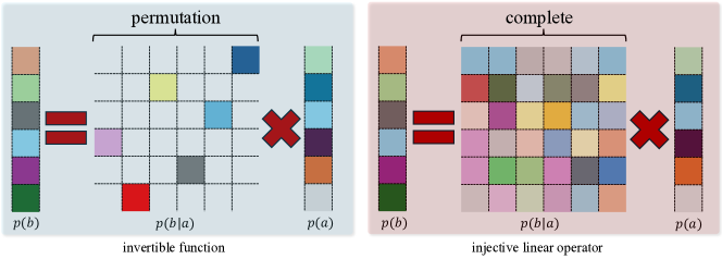
Figure 6: Invertible function vs. injective linear operator. Consider two variables $a$ and $b$ connected by the function $b=g(a)$, where $g$ is invertible. Alternatively, their relationship can be expressed as $p(b)=L_{b\mid a}\circ p(a)$, where $L_{b\mid a}$ is an injective linear operator. The grid represents $p(b\mid a)$, with color indicating non-zero values and white representing zero. Intuitively, in the discrete case, a full-rank operator corresponds to this relationship. An invertible function implies an injective linear operator, but not vice versa.

Appendix B Extended Related Work

Causal discovery algorithms in climate.

A prominent approach for causal discovery in climate analysis is PCMCI (Runge et al., 2019), which is specifically designed for linearly dependent time-series data. PCMCI effectively captures time-lagged dependencies and instantaneous relationships. Subsequently,  (Runge, 2020) extended this method to handle nonlinear scenarios. However, these methods do not account for latent variables, which limits their ability to accurately model real-world climate systems. Recently, several causal representation learning methods inspired by climate science have been developed. For example,  (Brouillard et al., ) assumes single-node structures to achieve identifiability, while  (Yao et al., 2024) employs an ODE-based approach to gain insights into climate-zone classification. Nevertheless, these approaches still overlook the dependencies among observed variables.

Comparisons with Jacobian-based methods.

Nonlinear causal discovery methods often leverage the Jacobian matrix or its byproduct to identify DAGs and ensure identifiability. For example, LiNGAM (Shimizu et al., 2006) uses a mixing matrix in linear settings, while (Lachapelle et al., 2019) and (Rolland et al., 2022) apply the Jacobian to nonlinear models for acyclicity constraints. In dynamical systems, (Atanackovic et al., 2024) adopt a Bayesian approach using Jacobians of SEMs, and (Zheng et al., 2023) learn Markov structures using the Jacobian of the data generation process. Jacobian properties also support identifiability in IMA (Gresele et al., 2021) and causal models with non-i.i.d. data (Reizinger et al., 2023), while (Liu et al., 2024) handle mixed models with score-based method. Table 5 summarizes these methods against our approach.

Method	$f$	Data	$J$	CD	CRL	Identifiability
(Shimizu et al., 2006)	Linear	Non-Gaussian	$J_{f^{-1}}$	✓	$\times$	✓
(Lachapelle et al., 2019)	Additive	Gaussian	$J_{f^{-1}}$	✓	$\times$	$\times$
(Gresele et al., 2021)	IMA	All	$J_{f}$	$\times$	$\times$	✓
(Zheng et al., 2023)	Sparse	All	$J_{f}$	$\times$	$\times$	✓
(Rolland et al., 2022)	Additive	Gaussian	$J_{\nabla_{x}\log p(x)}$	✓	$\times$	$\times$
(Atanackovic et al., 2024)	Cyclic (ODE)	All	$J_{f}$	✓	$\times$	$\times$
(Reizinger et al., 2023)	All	Assums. 2, F. 1	$J_{f^{-1}}$	✓	$\times$	✓
(Liu et al., 2024)	Mixed	Gaussian	$J_{\nabla_{x}\log p(x)}$	✓	$\times$	Partial
Ours	All	All	$J_{f^{-1}}$	✓	✓	✓

Table 5: Comparison of different methods based on their property in function type ($f$), data, Jacobian ($J$), causal discovery (CD), causal represnetation learning (CRL), and achievement of identifiability.

Appendix C Experiment Details

C.1 On Simulation Dataset

Evaluation metrics.

Due to the nature of monoblock identifiability descipted in Theorem 3.2, we use the coefficient of determination $R^{2}$ between the estimated variables $\hat{\mathbf{z}}_{t}$ and the true variables $\mathbf{z}_{t}$, where $R^{2}=1$ indicates perfect alignment. We employ kernel regression with a Gaussian kernel to estimate the nonlinear mapping. For recovering latent components in Theorem 3.3), we apply the Spearman Mean Correlation Coefficient (MCC). We use the Structural Hamming Distance (SHD) to evaluate similarity of learned latent and observed causal structure. Specifically, considering the indeterminacy of the permutation of identified latent variables, we align the instantaneous latent causal structure $\mathbf{J}_{r}(\hat{\mathbf{z}}_{t})$ and time-lagged latent causal structure $\mathbf{J}_{r}(\hat{\mathbf{z}}_{t-1})$ by permuting the learned adjacency matrices to match the ground truth. As a surrogate metric to learn observed causal DAG, we evaluated recovery of $\mathbf{s}_{t}$ using unpermuted MCC, corresponding to the identification strategy shown in Theorem 3.8. The recovered observed and latent causal DAG are further evaluated using SHD, divided by the number of possible structures. Based on such evaluation process, we also report TPR (recall), precision, and F1 among the comparisons with constraint-based methods.

Simulation process

As defined in Def 2.2, under the Independent setting for the latent temporal process and dependent noise variable $\mathbf{s}_{t}$, we use the generation process from (Yao et al., 2022). For observational causal relations, we randomly generate lower triangular matrices and apply equal row and column permutations to obtain a mixing structure, which is combined with an MLP network generated from $\mathbf{z}_{t}$ and $\mathbf{s}_{t}$ using LeakyReLU units. This simulation is also used for Sparse and Dense settings, controlling graph degree after removing diagonals. Each independent noise is sampled from normal distributions.

Baselines implementation details.

We utilized publicly available implementations for TDRL, CaRiNG, and iCRITIS, covering the majority of the employed methods. As G-CaRL’s code was not released, we re-implemented it based on the details provided in the original paper. Additionally, since the iCRITIS setup was originally designed for image inputs, we adapted it by replacing its encoder and decoder components with a Variational Autoencoder with same hyperparameters in NCDL.

Mask by inductive bias.

Continuous optimization faces challenges like local minima (Ng et al., 2022; Maddison et al., 2017), making it difficult to scale to higher dimensions. However, incorporating prior knowledge on the low probability of certain dependencies (Spirtes et al., 2001; Runge et al., 2019) enables us to compute a mask. To validate this approach using physical laws as observed DAG initialization  C.2 in climate data, we mask $\frac{3}{4}$ of the lower triangular elements in a simulation with $d_{x}=100$, a ratio much lower than in real-world applications.

Comparison with constraint-based methods.

Constraint-based methods rely on Conditional Independence (CI) tests and do not require a specified form of structural equation models (SEMs), making them a nonparametric approach. However, CI test-based methods generally return equivalence classes of graphs rather than a unique solution. For example, algorithms such as FCI produce Partial Ancestral Graphs (PAGs), and CD-NOD similarly yields equivalence classes. In our implementation, we utilize the Causal-learn package (Zheng et al., 2024) for FCI and CD-NOD and the Tigramite library (Runge et al., 2019) for PCMCI and LPCMCI. We employ a near-optimal configuration for these methods to facilitate fair comparisons. The details for each method are as follows:

1. FCI: We use Fisher’s Z conditional independence test. For the obtained PAG, we enumerate all possible adjacency matrices and select the one closest to the ground truth by minimizing the Structural Hamming Distance (SHD).

2. CD-NOD: We concatenate the time indices $[1,2,\ldots,T]$ of the simulated data into the observed variables and only consider the edges that exclude the time index. We use kernel-based CI test since it demonstrates superior performance here. We consider all obtained equivalence classes and select the result that minimizes SHD relative to the ground truth.

3. PCMCI: We use partial correlation as the metric of conditional independent test. We enforce no time-lagged relationships in PCMCI and run it to focus exclusively on contemporaneous (instantaneous) causal relationships. In the Tigramite library, this can be achieved by setting the maximum time lag $\tau_{\text{max}}$ to zero. This effectively disables the search for lagged causal dependencies. We select contemporary relationships as the ultimate result.

4. LPCMCI: Similarly to PCMCI, we use partial correlation as the metric of conditional independent test, and select the contemporary relationships as the causal graph obtained.

Study on dimension of latent variables.

We fix $d_{x}=6$ and vary $d_{z}=\{2,3,4\}$ as shown in Table 6. The results indicate that both the Markov network and time-lagged structure are identifiable for lower dimensions. However, as the latent dimension increases, there is a decline in identifiability of the latent structure, highlighting ongoing challenges in the continuous optimization of latent process identification (Zhang et al., 2024; Li et al., 2024). Nevertheless, monoblock identifiability ($R^{2}$) remains satisfied across all settings.

$d_{x}$	$d_{z}$	SHD ($\mathcal{G}_{x_{t}}$)	TPR	Precision	MCC ($\mathbf{s}_{t}$)	MCC ($\mathbf{z}_{t}$)	SHD ($\mathcal{G}_{z_{t}}$)	SHD ($\mathcal{M}_{lag}$)	$R^{2}$
6	2	0.12 ($\pm$0.04)	0.86 ($\pm$0.02)	0.85 ($\pm$0.04)	0.9864 ($\pm$0.01)	0.9741 ($\pm$0.03)	0.15 ($\pm$0.03)	0.21 ($\pm$0.05)	0.95 ($\pm$0.01)
	3	0.18 ($\pm$0.06)	0.83 ($\pm$0.02)	0.80 ($\pm$0.04)	0.9583 ($\pm$0.02)	0.9505 ($\pm$0.01)	0.24 ($\pm$0.06)	0.33 ($\pm$0.09)	0.92 ($\pm$0.01)
	4	0.23 ($\pm$0.02)	0.80 ($\pm$0.06)	0.74 ($\pm$0.01)	0.9041 ($\pm$0.02)	0.8931 ($\pm$0.03)	0.33 ($\pm$0.03)	0.48 ($\pm$0.05)	0.91 ($\pm$0.02)

Table 6: Results on different latent dimensions. We run simulations with 5 random seeds, selected based on the best-converged results to avoid local minima.

Ablation study on conditions.

Setting	MCC ($\mathbf{s}_{t}$)	$R^{2}$
A	0.6328	0.34
B	0.7563	0.67
C	0.7052	0.85

Table 7: Assumption ablation study. We mainly present these result to verify the necessity of our assumptions.

We further validate our identifiability theory using $d_{z}=3$ and $d_{x}=6$. In simulating data, we remove conditionsthat are nontrivial to our theories, including:

1. A (Def. 2.1): Ensuring $\mathbf{z}_{t}$ conditionally independent and replacing the transition function with an orthogonal matrix, violating the 3-measurement Hu & Schennach (2008).

2. B (Assumption b)): Violating the injectivity of linear operators using $g_{s}$: $\mathbf{z}_{t}=\mathbf{z}_{t-1}+\bm{\epsilon}_{z_{t}}$, where $\bm{\epsilon}_{z_{t}}\sim\text{Uniform}(0,1)$ is a typical violation Mattner (1993) for injectivity of $L_{z_{t}\mid z_{t-1}}$, as well as $L_{x_{t-1}\mid x_{t+1}}$.

3. C (Assumption 3.8): Violating the generation variability assumption with $\mathbf{s}_{t}=q(\mathbf{z}_{t})+\bm{\epsilon}_{x_{t}}$, where $\bm{\epsilon}_{x_{t}}\sim\mathcal{N}(0,\mathbf{I}_{d_{x}})$ and $q$ is a mixing process, results in a linear additive Gaussian model without heteroscedasticity. Such a setup significantly reduces variability, as discussed in Yao et al. (2022)..

As shown in Table 7, without these assumptions, we cannot achieve monoblock identifiability or identify the observed causal DAG, leading to a decrease in $R^{2}$ and MCC ($\mathbf{s}_{t}$). In summary, these results further confirm the validity of our theory and the necessity of these assumptions, especially under challenging conditions where they are disrupted.

Hyperparameter sensitivity.

We test the hyperparameter sensitivity of NCDL w.r.t. the sparsity and DAG penalty, as these hyperparameters have a significant influence on the performance of structure learning. In this experiment, we set $d_{z}=3$ and $d_{z}=6$. As shown in Table 8, the results demonstrate robustness across different settings, although the performance of structure learning is particularly sensitive to the sparsity constraint.

$\alpha$	$1\times 10^{-5}$	$5\times 10^{-5}$	$1\times 10^{-4}$	$5\times 10^{-4}$	$1\times 10^{-3}$	$1\times 10^{-2}$
SHD	0.23	0.22	0.18	0.27	0.32	0.67
$\beta$	$1\times 10^{-5}$	$5\times 10^{-5}$	$1\times 10^{-4}$	$5\times 10^{-4}$	$1\times 10^{-3}$	$1\times 10^{-2}$
SHD	0.37	0.18	0.20	/	/	/

Table 8: Hyperparameter sensitivity. We run experiments using 5 different random seeds for data generation and estimation procedures, reporting the average performance on evaluation metrics. ”/” indicates loss explosion. Notably, an excessively large DAG penalty at the beginning of training can result in a loss explosion or the failure of convergence.

C.2 On Real-world Dataset

CESM2 Pacific SST.

CESM2 dataset employs monthly Sea Surface Temperature (SST) data generated from a $500$-year pre-$2020$ control run of the CESM2 climate model. The dataset is restricted to oceanic regions, excluding all land areas, and retains its native gridded structure to preserve spatial correlations. It encompasses $6000$ temporal steps, representing monthly SST values over the designated period. Spatially, the dataset comprises a grid with 186 latitude points and $151$ longitude points, resulting in $28086$ spatial variables, including $3337$ land points where SST is undefined, and $24749$ valid SST observations. To accommodate computational constraints, a downsampled version of the data, reduced to 84 grid points ($6\times 14$), is utilized.

WeatherBench (Rasp et al., 2020).

WeatherBench is a benchmark dataset specifically tailored for data-driven weather forecasting. We specifically selected wind direction data for visualization comparisons within the same time period, maintaining the original 350,640 timestamps. Wind system is considered as the dominating factor resulting in potential instantaneous causal relationships among the temperature in different regions.

Initialization observed DAG.

We incorporate the Spatial Autoregressive (SAR) model as a prior in the continuous optimization of the causal DAG structure matrix $G_{\hat{x}_{t}}$ to mitigate local minima. The SAR model, commonly used in geography, economics, and environmental science, captures spatial dependencies defined as $\mathbf{X}=\mathbf{Z}\beta+\lambda\mathbf{W}\mathbf{X}+\mathbf{E}$, where $\mathbf{W}$ is the spatial weights matrix, and $\mathbf{E}$ is a disturbance term. Setting $\beta=0$ results in a pure SAR model: $\mathbf{X}=\lambda\mathbf{W}\mathbf{X}+\mathbf{E}.$ We define $\mathbf{W}$ based on Euclidean distances constrained by $\mathcal{M}_{loc}$, where $[\mathcal{M}_{loc}]_{i,j}=1\{\|s_{2}-s_{1}\|_{2}\leq 50\}$, with $s_{1}$ and $s_{2}$ representing the locations of two regions. The rationale is that regions cannot be instantaneously connected if they are separated by a large physical distance. This configuration captures potential instantaneous causal effects only between spatially adjacent regions within a specified distance threshold of 50 units.

Observed causal DAG in climate system.

In addition to using the mask gradient-based method for mask estimation, we compute the causal DAG by: $\hat{\mathcal{G}}_{x_{t}}=\text{supp}(\hat{\mathcal{M}}_{x_{t}}*\mathbf{J}_{\hat{g}}(\mathbf{x}_{t})*\mathcal{M}_{init})$. A threshold of 0.15 is applied to obtain the final binary adjacency matrix. To compute the partial Jacobian $\mathbf{J}_{\hat{g}}(\mathbf{x}_{t})$ with respect to $\mathbf{s}_{t}$ while holding $\mathbf{z}_{t}$ constant, set requires_grad=False for $\mathbf{z}_{t}$, and use autograd.functional.jacobian in PyTorch.

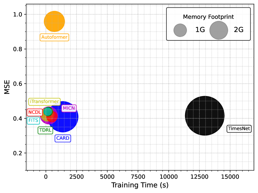
Figure 7: Comparison of computational cost. Different colors represent different methods, while the size of the circles corresponds to memory usage. The prediction length is set to 96.

Runtime and computational efficiency.

We report the computational cost of the different methods considered. The comparison considers metrics including training time, memory usage, and corresponding performance MSE in forecasting task. Note that inference time is not included in the comparison, as our work focuses on causal structure learning through continuous optimization rather than constraint-based methods. Fig. 7 shows that our NCDL method simultaneously learns the causal structure while achieving the lowest MSE, highlighting the importance of building a transparent and interpretable model. Furthermore, NCDL exhibits similar training time and memory usage compared to mainstream time-series forecasting models in the lightweight track.

References

- Abbass et al. (2022) Kashif Abbass, Muhammad Zeeshan Qasim, Huaming Song, Muntasir Murshed, Haider Mahmood, and Ijaz Younis. A review of the global climate change impacts, adaptation, and sustainable mitigation measures. Environmental Science and Pollution Research, 29(28):42539–42559, 2022.
- Atanackovic et al. (2024) Lazar Atanackovic, Alexander Tong, Bo Wang, Leo J Lee, Yoshua Bengio, and Jason S Hartford. Dyngfn: Towards bayesian inference of gene regulatory networks with gflownets. Advances in Neural Information Processing Systems, 36, 2024.
- Boé & Terray (2014) Julien Boé and Laurent Terray. Land–sea contrast, soil-atmosphere and cloud-temperature interactions: interplays and roles in future summer european climate change. Climate dynamics, 42(3):683–699, 2014.
- (4) Philippe Brouillard, Sebastien Lachapelle, Julia Kaltenborn, Yaniv Gurwicz, Dhanya Sridhar, Alexandre Drouin, Peer Nowack, Jakob Runge, and David Rolnick. Causal representation learning in temporal data via single-parent decoding.
- Buchholz et al. (2024) Simon Buchholz, Goutham Rajendran, Elan Rosenfeld, Bryon Aragam, Bernhard Schölkopf, and Pradeep Ravikumar. Learning linear causal representations from interventions under general nonlinear mixing. Advances in Neural Information Processing Systems, 36, 2024.
- Carroll et al. (2010) Raymond J Carroll, Xiaohong Chen, and Yingyao Hu. Identification and estimation of nonlinear models using two samples with nonclassical measurement errors. Journal of nonparametric statistics, 22(4):379–399, 2010.
- Chen et al. (2024) Guangyi Chen, Yifan Shen, Zhenhao Chen, Xiangchen Song, Yuewen Sun, Weiran Yao, Xiao Liu, and Kun Zhang. Caring: Learning temporal causal representation under non-invertible generation process. arXiv preprint arXiv:2401.14535, 2024.
- Chen & Wang (1995) Yi-Leng Chen and Jian-Jian Wang. The effects of precipitation on the surface temperature and airflow over the island of hawaii. Monthly weather review, 123(3):681–694, 1995.
- Chernozhukov et al. (2007) Victor Chernozhukov, Guido W Imbens, and Whitney K Newey. Instrumental variable estimation of nonseparable models. Journal of Econometrics, 139(1):4–14, 2007.
- Dunford & Schwartz (1988) Nelson Dunford and Jacob T Schwartz. Linear operators, part 1: general theory, volume 10. John Wiley & Sons, 1988.
- D’Haultfoeuille (2011) Xavier D’Haultfoeuille. On the completeness condition in nonparametric instrumental problems. Econometric Theory, 27(3):460–471, 2011.
- Ebert-Uphoff & Deng (2012) Imme Ebert-Uphoff and Yi Deng. Causal discovery for climate research using graphical models. Journal of Climate, 25(17):5648–5665, 2012.
- Freeman (1983) John R Freeman. Granger causality and the times series analysis of political relationships. American Journal of Political Science, pp. 327–358, 1983.
- Gassiat et al. (2020) Elisabeth Gassiat, Sylvain Le Corff, and Luc Lehéricy. Identifiability and consistent estimation of nonparametric translation hidden markov models with general state space. Journal of Machine Learning Research, 21(115):1–40, 2020.
- Gerhardus & Runge (2020) Andreas Gerhardus and Jakob Runge. High-recall causal discovery for autocorrelated time series with latent confounders. Advances in Neural Information Processing Systems, 33:12615–12625, 2020.
- Gresele et al. (2021) Luigi Gresele, Julius Von Kügelgen, Vincent Stimper, Bernhard Schölkopf, and Michel Besserve. Independent mechanism analysis, a new concept? Advances in neural information processing systems, 34:28233–28248, 2021.
- Hälvä et al. (2021) Hermanni Hälvä, Sylvain Le Corff, Luc Lehéricy, Jonathan So, Yongjie Zhu, Elisabeth Gassiat, and Aapo Hyvarinen. Disentangling identifiable features from noisy data with structured nonlinear ica. Advances in Neural Information Processing Systems, 34:1624–1633, 2021.
- Hoyer et al. (2008) Patrik Hoyer, Dominik Janzing, Joris M Mooij, Jonas Peters, and Bernhard Schölkopf. Nonlinear causal discovery with additive noise models. Advances in neural information processing systems, 21, 2008.
- Hu (2008) Yingyao Hu. Identification and estimation of nonlinear models with misclassification error using instrumental variables: A general solution. Journal of Econometrics, 144(1):27–61, 2008.
- Hu & Schennach (2008) Yingyao Hu and Susanne M Schennach. Instrumental variable treatment of nonclassical measurement error models. Econometrica, 76(1):195–216, 2008.
- Hu & Shiu (2018) Yingyao Hu and Ji-Liang Shiu. Nonparametric identification using instrumental variables: sufficient conditions for completeness. Econometric Theory, 34(3):659–693, 2018.
- Hu & Shum (2012) Yingyao Hu and Matthew Shum. Nonparametric identification of dynamic models with unobserved state variables. Journal of Econometrics, 171(1):32–44, 2012.
- Huang et al. (2019) Biwei Huang, Kun Zhang, Mingming Gong, and Clark Glymour. Causal discovery and forecasting in nonstationary environments with state-space models. In International conference on machine learning, pp. 2901–2910. Pmlr, 2019.
- Huang et al. (2020) Biwei Huang, Kun Zhang, Jiji Zhang, Joseph Ramsey, Ruben Sanchez-Romero, Clark Glymour, and Bernhard Schölkopf. Causal discovery from heterogeneous/nonstationary data. Journal of Machine Learning Research, 21(89):1–53, 2020.
- Huang et al. (2022) Biwei Huang, Charles Jia Han Low, Feng Xie, Clark Glymour, and Kun Zhang. Latent hierarchical causal structure discovery with rank constraints. Advances in neural information processing systems, 35:5549–5561, 2022.
- Hyvarinen & Morioka (2016) Aapo Hyvarinen and Hiroshi Morioka. Unsupervised feature extraction by time-contrastive learning and nonlinear ica. Advances in neural information processing systems, 29, 2016.
- Hyvarinen & Morioka (2017) Aapo Hyvarinen and Hiroshi Morioka. Nonlinear ica of temporally dependent stationary sources. In Artificial Intelligence and Statistics, pp. 460–469. PMLR, 2017.
- Hyvärinen & Pajunen (1999) Aapo Hyvärinen and Petteri Pajunen. Nonlinear independent component analysis: Existence and uniqueness results. Neural networks, 12(3):429–439, 1999.
- Hyvarinen et al. (2019) Aapo Hyvarinen, Hiroaki Sasaki, and Richard Turner. Nonlinear ica using auxiliary variables and generalized contrastive learning. In The 22nd International Conference on Artificial Intelligence and Statistics, pp. 859–868. PMLR, 2019.
- Hyvärinen et al. (2023) Aapo Hyvärinen, Ilyes Khemakhem, and Hiroshi Morioka. Nonlinear independent component analysis for principled disentanglement in unsupervised deep learning. Patterns, 4(10), 2023.
- Jang et al. (2017) Eric Jang, Shixiang Gu, and Ben Poole. Categorical reparameterization with Gumbel-Softmax. In International Conference on Learning Representations, 2017.
- Khemakhem et al. (2020) Ilyes Khemakhem, Diederik Kingma, Ricardo Monti, and Aapo Hyvarinen. Variational autoencoders and nonlinear ica: A unifying framework. In International Conference on Artificial Intelligence and Statistics, pp. 2207–2217. PMLR, 2020.
- Klindt et al. (2020) David Klindt, Lukas Schott, Yash Sharma, Ivan Ustyuzhaninov, Wieland Brendel, Matthias Bethge, and Dylan Paiton. Towards nonlinear disentanglement in natural data with temporal sparse coding. arXiv preprint arXiv:2007.10930, 2020.
- Kong et al. (2023) Lingjing Kong, Biwei Huang, Feng Xie, Eric Xing, Yuejie Chi, and Kun Zhang. Identification of nonlinear latent hierarchical models. Advances in Neural Information Processing Systems, 36:2010–2032, 2023.
- Kress et al. (1989) Rainer Kress, Vladimir Maz’ya, and Vladimir Kozlov. Linear integral equations, volume 82. Springer, 1989.
- Lachapelle et al. (2019) Sébastien Lachapelle, Philippe Brouillard, Tristan Deleu, and Simon Lacoste-Julien. Gradient-based neural dag learning. arXiv preprint arXiv:1906.02226, 2019.
- Lachapelle et al. (2022) Sébastien Lachapelle, Pau Rodriguez, Yash Sharma, Katie E Everett, Rémi Le Priol, Alexandre Lacoste, and Simon Lacoste-Julien. Disentanglement via mechanism sparsity regularization: A new principle for nonlinear ica. In Conference on Causal Learning and Reasoning, pp. 428–484. PMLR, 2022.
- Lemeire & Janzing (2013) Jan Lemeire and Dominik Janzing. Replacing causal faithfulness with algorithmic independence of conditionals. Minds and Machines, 23:227–249, 2013.
- Li et al. (2024) Zijian Li, Yifan Shen, Kaitao Zheng, Ruichu Cai, Xiangchen Song, Mingming Gong, Zhifeng Hao, Zhengmao Zhu, Guangyi Chen, and Kun Zhang. On the identification of temporally causal representation with instantaneous dependence. arXiv preprint arXiv:2405.15325, 2024.
- Lin (1997) Juan Lin. Factorizing multivariate function classes. Advances in neural information processing systems, 10, 1997.
- Lippe et al. (2022) Phillip Lippe, Sara Magliacane, Sindy Löwe, Yuki M Asano, Taco Cohen, and Efstratios Gavves. Causal representation learning for instantaneous and temporal effects in interactive systems. arXiv preprint arXiv:2206.06169, 2022.
- Liu et al. (2024) Wenqin Liu, Biwei Huang, Erdun Gao, Qiuhong Ke, Howard Bondell, and Mingming Gong. Causal discovery with mixed linear and nonlinear additive noise models: A scalable approach. In Causal Learning and Reasoning, pp. 1237–1263. PMLR, 2024.
- Locatello et al. (2019) Francesco Locatello, Stefan Bauer, Mario Lucic, Gunnar Raetsch, Sylvain Gelly, Bernhard Schölkopf, and Olivier Bachem. Challenging common assumptions in the unsupervised learning of disentangled representations. In international conference on machine learning, pp. 4114–4124. PMLR, 2019.
- Long et al. (2023) Stephanie Long, Alexandre Piché, Valentina Zantedeschi, Tibor Schuster, and Alexandre Drouin. Causal discovery with language models as imperfect experts. arXiv preprint arXiv:2307.02390, 2023.
- Lucarini et al. (2014) Valerio Lucarini, Richard Blender, Corentin Herbert, Francesco Ragone, Salvatore Pascale, and Jeroen Wouters. Mathematical and physical ideas for climate science. Reviews of Geophysics, 52(4):809–859, 2014.
- Maddison et al. (2017) Chris J. Maddison, Andriy Mnih, and Yee Whye Teh. The concrete distribution: A continuous relaxation of discrete random variables. In International Conference on Learning Representations, 2017.
- Mattner (1993) Lutz Mattner. Some incomplete but boundedly complete location families. The Annals of Statistics, pp. 2158–2162, 1993.
- Monti et al. (2020) Ricardo Pio Monti, Kun Zhang, and Aapo Hyvärinen. Causal discovery with general non-linear relationships using non-linear ica. In Uncertainty in artificial intelligence, pp. 186–195. PMLR, 2020.
- Morioka & Hyvärinen (2023) Hiroshi Morioka and Aapo Hyvärinen. Causal representation learning made identifiable by grouping of observational variables. arXiv preprint arXiv:2310.15709, 2023.
- Newey & Powell (2003) Whitney K Newey and James L Powell. Instrumental variable estimation of nonparametric models. Econometrica, 71(5):1565–1578, 2003.
- (51) Ignavier Ng, Xinshuai Dong, Haoyue Dai, Biwei Huang, Peter Spirtes, and Kun Zhang. Score-based causal discovery of latent variable causal models. In Forty-first International Conference on Machine Learning.
- Ng et al. (2022) Ignavier Ng, Shengyu Zhu, Zhuangyan Fang, Haoyang Li, Zhitang Chen, and Jun Wang. Masked gradient-based causal structure learning. In Proceedings of the 2022 SIAM International Conference on Data Mining (SDM), pp. 424–432. SIAM, 2022.
- Paulson & Simpson (1981) CA Paulson and JJ Simpson. The temperature difference across the cool skin of the ocean. Journal of Geophysical Research: Oceans, 86(C11):11044–11054, 1981.
- Pearl (2009) Judea Pearl. Causality. Cambridge university press, 2009.
- Peters et al. (2017) Jonas Peters, Dominik Janzing, and Bernhard Schölkopf. Elements of causal inference: foundations and learning algorithms. The MIT Press, 2017.
- Rasp et al. (2020) Stephan Rasp, Peter D Dueben, Sebastian Scher, Jonathan A Weyn, Soukayna Mouatadid, and Nils Thuerey. Weatherbench: a benchmark data set for data-driven weather forecasting. Journal of Advances in Modeling Earth Systems, 12(11):e2020MS002203, 2020.
- Reizinger et al. (2023) Patrik Reizinger, Yash Sharma, Matthias Bethge, Bernhard Schölkopf, Ferenc Huszár, and Wieland Brendel. Jacobian-based causal discovery with nonlinear ica. Transactions on Machine Learning Research, 2023.
- Rezende & Mohamed (2015) Danilo Rezende and Shakir Mohamed. Variational inference with normalizing flows. In International conference on machine learning, pp. 1530–1538. PMLR, 2015.
- Rolland et al. (2022) Paul Rolland, Volkan Cevher, Matthäus Kleindessner, Chris Russell, Dominik Janzing, Bernhard Schölkopf, and Francesco Locatello. Score matching enables causal discovery of nonlinear additive noise models. In International Conference on Machine Learning, pp. 18741–18753. PMLR, 2022.
- Rolnick et al. (2022) David Rolnick, Priya L Donti, Lynn H Kaack, Kelly Kochanski, Alexandre Lacoste, Kris Sankaran, Andrew Slavin Ross, Nikola Milojevic-Dupont, Natasha Jaques, Anna Waldman-Brown, et al. Tackling climate change with machine learning. ACM Computing Surveys (CSUR), 55(2):1–96, 2022.
- Runge (2020) Jakob Runge. Discovering contemporaneous and lagged causal relations in autocorrelated nonlinear time series datasets. In Conference on Uncertainty in Artificial Intelligence, pp. 1388–1397. Pmlr, 2020.
- Runge et al. (2019) Jakob Runge, Peer Nowack, Marlene Kretschmer, Seth Flaxman, and Dino Sejdinovic. Detecting and quantifying causal associations in large nonlinear time series datasets. Science advances, 5(11):eaau4996, 2019.
- Schölkopf et al. (2021) Bernhard Schölkopf, Francesco Locatello, Stefan Bauer, Nan Rosemary Ke, Nal Kalchbrenner, Anirudh Goyal, and Yoshua Bengio. Toward causal representation learning. Proceedings of the IEEE, 109(5):612–634, 2021.
- Shimizu et al. (2006) Shohei Shimizu, Patrik O Hoyer, Aapo Hyvärinen, Antti Kerminen, and Michael Jordan. A linear non-gaussian acyclic model for causal discovery. Journal of Machine Learning Research, 7(10), 2006.
- Silva et al. (2006) Ricardo Silva, Richard Scheines, Clark Glymour, Peter Spirtes, and David Maxwell Chickering. Learning the structure of linear latent variable models. Journal of Machine Learning Research, 7(2), 2006.
- Silva et al. (2012) Ricardo Silva, Richard Scheines, Clark Glymour, and Peter L Spirtes. Learning measurement models for unobserved variables. arXiv preprint arXiv:1212.2516, 2012.
- Spantini et al. (2018) Alessio Spantini, Daniele Bigoni, and Youssef Marzouk. Inference via low-dimensional couplings. The Journal of Machine Learning Research, 19(1):2639–2709, 2018.
- Spearman (1928) Charles Spearman. Pearson’s contribution to the theory of two factors. British Journal of Psychology, 19(1):95, 1928.
- Spirtes et al. (2001) Peter Spirtes, Clark Glymour, and Richard Scheines. Causation, prediction, and search. MIT press, 2001.
- Stips et al. (2016) Adolf Stips, Diego Macias, Clare Coughlan, Elisa Garcia-Gorriz, and X San Liang. On the causal structure between co2 and global temperature. Scientific reports, 6(1):21691, 2016.
- Vautard et al. (2019) Robert Vautard, Geert Jan Van Oldenborgh, Friederike EL Otto, Pascal Yiou, Hylke De Vries, Erik Van Meijgaard, Andrew Stepek, Jean-Michel Soubeyroux, Sjoukje Philip, Sarah F Kew, et al. Human influence on european winter wind storms such as those of january 2018. Earth System Dynamics, 10(2):271–286, 2019.
- Xie et al. (2020) Feng Xie, Ruichu Cai, Biwei Huang, Clark Glymour, Zhifeng Hao, and Kun Zhang. Generalized independent noise condition for estimating latent variable causal graphs. Advances in neural information processing systems, 33:14891–14902, 2020.
- Yao et al. (2023) Dingling Yao, Danru Xu, Sébastien Lachapelle, Sara Magliacane, Perouz Taslakian, Georg Martius, Julius von Kügelgen, and Francesco Locatello. Multi-view causal representation learning with partial observability. arXiv preprint arXiv:2311.04056, 2023.
- Yao et al. (2024) Dingling Yao, Caroline Muller, and Francesco Locatello. Marrying causal representation learning with dynamical systems for science. arXiv preprint arXiv:2405.13888, 2024.
- Yao et al. (2021) Weiran Yao, Yuewen Sun, Alex Ho, Changyin Sun, and Kun Zhang. Learning temporally causal latent processes from general temporal data. arXiv preprint arXiv:2110.05428, 2021.
- Yao et al. (2022) Weiran Yao, Guangyi Chen, and Kun Zhang. Temporally disentangled representation learning. Advances in Neural Information Processing Systems, 35:26492–26503, 2022.
- Yu et al. (2019) Yue Yu, Jie Chen, Tian Gao, and Mo Yu. Dag-gnn: Dag structure learning with graph neural networks. In International Conference on Machine Learning, pp. 7154–7163. PMLR, 2019.
- Zhang (2013) Jiji Zhang. A comparison of three occam’s razors for markovian causal models. The British journal for the philosophy of science, 2013.
- Zhang & Hyvarinen (2012) Kun Zhang and Aapo Hyvarinen. On the identifiability of the post-nonlinear causal model. arXiv preprint arXiv:1205.2599, 2012.
- Zhang et al. (2012) Kun Zhang, Bernhard Schölkopf, and Dominik Janzing. Invariant gaussian process latent variable models and application in causal discovery. arXiv preprint arXiv:1203.3534, 2012.
- Zhang et al. (2024) Kun Zhang, Shaoan Xie, Ignavier Ng, and Yujia Zheng. Causal representation learning from multiple distributions: A general setting. arXiv preprint arXiv:2402.05052, 2024.
- Zheng & Zhang (2023) Yujia Zheng and Kun Zhang. Generalizing nonlinear ica beyond structural sparsity. Advances in Neural Information Processing Systems, 36:13326–13355, 2023.
- Zheng et al. (2022) Yujia Zheng, Ignavier Ng, and Kun Zhang. On the identifiability of nonlinear ica: Sparsity and beyond. Advances in neural information processing systems, 35:16411–16422, 2022.
- Zheng et al. (2023) Yujia Zheng, Ignavier Ng, Yewen Fan, and Kun Zhang. Generalized precision matrix for scalable estimation of nonparametric markov networks. arXiv preprint arXiv:2305.11379, 2023.
- Zheng et al. (2024) Yujia Zheng, Biwei Huang, Wei Chen, Joseph Ramsey, Mingming Gong, Ruichu Cai, Shohei Shimizu, Peter Spirtes, and Kun Zhang. Causal-learn: Causal discovery in python. Journal of Machine Learning Research, 25(60):1–8, 2024.