Degree-Based Logical Adjacency Checking (DBLAC): A Novel Heuristic for Vertex Coloring

Abstract

Degree Based Logical Adjacency Checking (DBLAC). An efficient coloring of graphs with unique logical AND operations. The logical AND operation shows More effective color assignment and fewer number of induced in the case of common edges between vertices. of colors used. In this work, we provide a detailed theoretical analysis of DBLAC’s time and space complexity. It furthermore shows its effectiveness through prolonged experiments on standard benchmark graphs. We still compare with existing algorithms namely DSATUR, and Recursive Largest First (RLF). Second, we show how DBLAC achieves competitive results with respect to both the number of colors used and runtime. performance.

Keywords: DSATUR Algorithm, RLF Algorithm, Graphs Theory, Chromatic, Graph Coloring. runtime efficiency, number, DIMACS Dataset, Optimization, Algorithm Performance, Vertex Coloring.

1 Introduction

The vertex coloring problem is a problem that assigns colors to the vertices of a graph so for every pair of adjacent vertices that share the same color. All vertices are the same color. Our goal is to reduce the number of colors used, called the chromatic number $\chi(G)$. It is computationally intractable for large particles, this problem is actually NP hard. graphs. Sometimes, heuristic algorithms tried to find approximate solution efficiently. In this paper, we present a new heuristic algorithm, Degree Based Logical Adjacency Check. In particular, building on a degree based ordering (DBLAC), but adding a new logical AND operation. to improve performance. The logical AND operation finds edges common to vertices. more efficient handling of color assignment. In particular this approach is ideal for dense and irregular graphs. where traditional heuristics are often difficult.

2 Related Work

Vertex coloring problem has been extensively studied, and many heuristics have been designed. It is proposed to solve it efficiently. We categorize these algorithms broadly into Greedy Heuristics, Recursive Partitioning Methods and Metaheuristics methods. We discuss the most notable algorithms, below. Finally, I discuss their time complexities and their mathematical foundations.

2.1 Greedy Heuristics

The simplest and most widely used approaches for vertex coloring are greedy heuristics. First, they give the vertices one by one color and no two adjacent vertices should have the same color. The criterion under which to select the next vertex to color is fixed [1].

2.1.1 Largest Degree First (LDF)

Vertices are ordered from smallest to largest in degree with degree being sorted using the Largest Degree First (LDF) Algorithm. colors them sequentially. Common intuition is that high degree vertices are more constrained, and therefore should be. First colored to minimize the number of colors needed [5].

Mathematical Formulation

Let $G=(V,E)$ be a graph with $n$ vertices and $m$ edges. The degree of a vertex $v$, denoted $\deg(v)$, is the number of edges incident to $v$. The LDF algorithm can be described as follows:

1. Sort vertices in descending order of degree: $V=\{v_{1},v_{2},\dots,v_{n}\}$ where $\deg(v_{1})\geq\deg(v_{2})\geq\dots\geq\deg(v_{n})$.

2. For each vertex $v_{i}$, assign the smallest available color not used by any of its neighbors.

Time Complexity

The time complexity of LDF is dominated by the sorting step, which takes $O(n\log n)$, and the color assignment step, which takes $O(n\Delta)$, where $\Delta$ is the maximum degree of the graph. Thus, the overall time complexity is:

$$O(n\log n+n\Delta)$$

In the worst case, $\Delta=n-1$, resulting in a time complexity of $O(n^{2})$.

2.1.2 DSATUR

DSATUR, is one of the best methods for coloring vertices in a very optimized way, which was introduced by Daniel Brélaz in 1979 [6]. DSATUR prioritizes vertices with maximum saturation degree, thus minimizing the number of colors needed to color the graph. For graphs with complex structures, particularly when the constraint is not known a priori, this approach performs well because it evolves with the coloring constraints during the execution.

Mathematical formulation

For a graph $G=(V,E)$ with $n$ vertices and $m$ edges, let $G$ be. In this case, the saturation degree of a vertex $v$, denoted $\text{sat}(v)$, is the number of distinct colors used in its neighbors. The DSATUR algorithm can be described as follows:

1. Additionally, all vertices are initialized with a saturation degree of 0.

2. Select at each step the vertex $v$ of maximum saturation degree. If the degrees of two vertices are the same, select the vertex with the highest degree.

3. Assign the smallest non-used color by any of $v$’s neighbors.

4. Update the saturation degrees of its uncolored neighbors $v$.

5. Repeat the process until all vertices are colored.

Time Complexity

The selection and color assignment steps dominate the time complexity of DSATUR. For each vertex, the algorithm must:

• Find a vertex with the maximum saturation degree, which takes $O(n)$ per step.

• Assign a color to its neighbors, and update the saturation degree of each neighbor. Given a maximum degree of the graph $\Delta$, this step takes $O(\Delta)$ per step.

Since there are $n$ vertices, the overall time complexity is:

$$O(n^{2}+n\Delta)$$

In the worst case, the $\Delta$ will be $n-1$, so we have $O(n^{2})$.

2.2 Recursive Partitioning Methods

Recursive partitioning methods divide the graph into independent sets (subsets of vertices with no edges between them) and color each set separately.

2.2.1 Recursive Largest First (RLF)

The Recursive Largest First (RLF), for solving the NP hard graph coloring problem. The idea was put forward by mathematician Frank Leighton in 1979[3]. In the RLF algorithm a graph is iteratively (considered to be sub optimally) solved by applying specialized heuristic rules to search for closed independent sets. The RLF algorithm is capable of producing exact solutions to special classes of graphs, for example to vertex bipartite graphs, cycle graphs and wheel graphs, thanks to these heuristics. Its main power here is its ability to reduce problem size, efficiently, by finding and coloring the largest independent sets recursively. In particular it is often very effective when the graph in question is sparse, because it tends to reduce the number of colors required to a mere anecdote. Moreover, the RLF algorithm is also deterministic, meaning the same input will make it obtainable the same result.

Mathematical Formulation

Let $G=(V,E)$ be a graph. The RLF algorithm can be described as follows:

1. While there are uncolored vertices:

   1. Construct an independent set $S$ by iteratively adding the vertex with the fewest neighbors in the remaining graph.

   2. Assign a new color to all vertices in $S$.

   3. Remove $S$ from the graph.

Time Complexity

RLF takes $O(n^{3})$ time, since for every iteration it takes $O(n^{2})$ steps to build the independent set. There are up to $n$ independent sets, and we aim to find an independent set efficiently.

2.3 Metaheuristics

Metaheuristics are high-level strategies that guide other heuristics to find approximate solutions. They are often used for complex or large-scale problems.They are particularly effective where most traditional algorithms or heuristics algorithms do not perform well enough due to vastness or the complexity of the search space.

2.3.1 Genetic Algorithms

Genetic algorithms (GAs) are inspired by natural selection and evolution. They maintain a population of candidate solutions and iteratively improve them using crossover, mutation, and selection operations.

Mathematical Formulation

Let $P$ be a population of candidate colorings. The GA can be described as follows:

1. Initialize $P$ with random colorings.

2. While the termination condition is not met:

   1. Select parents from $P$ based on fitness (e.g., number of colors used).

   2. Generate offspring by applying crossover and mutation.

   3. Replace the least fit individuals in $P$ with the offspring.

Time Complexity

The time complexity of GAs depends on the population size, the number of generations, and the complexity of the fitness function. In practice, GAs are computationally expensive and have a time complexity of $O(kn^{2})$, where $k$ is the number of generations.

2.4 Limitations of Existing Algorithms

While the above algorithms perform well in many cases, they have limitations:

• LDF and DSATUR struggle with dense graphs, where the number of edges is close to $\frac{n(n-1)}{2}$.

• RLF is computationally expensive and may not scale well to large graphs.

• Metaheuristics like GAs are time-consuming and may not guarantee optimal solutions.

2.5 Our Contribution: DBLAC

Our proposed algorithm, Degree-Based Logical Adjacency Checking (DBLAC), addresses these limitations by combining degree-based ordering with a logical AND operation to identify common edges between vertices. This approach enables more efficient color assignment, particularly for dense and irregular graphs. The logical AND operation is a novel feature that distinguishes DBLAC from existing algorithms.

Mathematical Formulation

Let $G=(V,E)$ be a graph. The DBLAC algorithm can be described as follows:

1. Order vertices in descending order of degree: $V=\{v_{1},v_{2},\dots,v_{n}\}$.

2. For each vertex $v_{i}$:

   1. Assign the smallest available color not used by any of its neighbors.

   2. Apply a logical AND operation to find common edges between $v_{i}$ and its neighbors.

   3. Assign colors to common vertices based on adjacency constraints.

Time Complexity

The time complexity of DBLAC is $O(n\Delta)$, where $\Delta$ is the maximum degree of the graph. This makes DBLAC more efficient than RLF and competitive with DSATUR and LDF.

3 Algorithm Description

Our algorithm, called Degree-Based Logical Adjacency Checking (DBLAC), works as follows:

Algorithm 1 Degree-Based Logical Adjacency Checking (DBLAC)

0: Graph $G=(V,E)$

0: Proper vertex coloring of $G$

1: Order vertices in descending order of degree: $V=\{v_{1},v_{2},\dots,v_{n}\}$

2: Initialize color set $C=\{c_{1},c_{2},\dots,c_{k}\}$ where $k$ is the maximum degree

3: for each vertex $v_{i}\in V$ do

4:  for each color $c_{j}\in C$ do

5:   if $c_{j}$ is not used by any adjacent vertex of $v_{i}$ then

6:    Assign $c_{j}$ to $v_{i}$

7:    Break

8:   end if

9:  end for

10:  Apply logical AND operation to find common edges between $v_{i}$ and its neighbors

11:  Assign colors to common vertices based on adjacency constraints

12: end for

3.1 Theoretical Analysis

3.1.1 Time Complexity

The time complexity of DBLAC is dominated by the adjacency-checking and logical AND operations. For each vertex, we check the colors of its neighbors, which takes $O(\Delta)$ time, where $\Delta$ is the maximum degree of the graph. The logical AND operation also takes $O(\Delta)$ time. Since there are $n$ vertices, the overall time complexity is:

$$O(n\Delta)$$

In the worst case, $\Delta=n-1$, resulting in a time complexity of $O(n^{2})$.

3.1.2 Space Complexity

The space complexity is determined by the storage required for the graph and the color assignments. The adjacency list representation of the graph requires $O(n+m)$ space, where $m$ is the number of edges. The color assignments require $O(n)$ space. Thus, the overall space complexity is:

$$O(n+m)$$

4 Application to Graph Problems

In this section, we apply DBLAC to three graph problems and demonstrate its effectiveness.

4.1 Problem 1: 5-Vertex Graph

Consider the graph shown in Figure 1.0 with five vertices. The vertices are ordered by degree as $\{v_{2},v_{1},v_{3},v_{4},v_{5}\}$.

4.1.1 Solution

• Assign $c_{1}$ to $v_{2}$ and $c_{2}$ to $v_{1}$.

• Check adjacency between $v_{2}$ and $v_{1}$. Since they are adjacent, they cannot share the same color.

• Apply logical AND operation to find common edges between $v_{2}$ and $v_{1}$, resulting in common vertices $v_{3}$ and $v_{5}$.

• Assign $c_{3}$ to $v_{3}$ and $v_{5}$.

• Assign $c_{2}$ to $v_{4}$.

4.1.2 Final Coloring

$$\{(v_{1},c_{2}),(v_{2},c_{1}),(v_{3},c_{3}),(v_{4},c_{2}),(v_{5},c_{3})\}$$

The graph is $\chi(3)$ Colors.

4.2 Problem 2: 6-Vertex Graph

Consider the graph shown in Figure 2.0 with six vertices. The vertices are ordered by degree as $\{f,a,d,c,e,b\}$.

4.2.1 Solution

• Assign $c_{1}$ to $f$ and $c_{2}$ to $a$.

• Check adjacency between $f$ and $a$. Since they are adjacent, they cannot share the same color.

• Apply logical AND operation to find common edges between $f$ and $a$, resulting in common vertices $\{b,c,d,e\}$.

• Assign $c_{3}$ to $d$ and $c_{4}$ to $c$.

• Assign $c_{4}$ to $e$.

• Assign $c_{3}$ to $b$.

4.2.2 Final Coloring

$$\{(a,c_{2}),(b,c_{3}),(c,c_{4}),(d,c_{3}),(e,c_{4}),(f,c_{1})\}$$

The graph is $\chi(4)$ Colors.

4.3 Problem 3: 6-Vertex Graph with Higher Complexity

Consider the graph shown in Figure 3.0 with six vertices. The vertices are ordered by degree as $\{v_{5},v_{1},v_{2},v_{3},v_{4},v_{6}\}$.

4.3.1 Solution

• Assign $c_{1}$ to $v_{5}$ and $c_{2}$ to $v_{1}$.

• Check adjacency between $v_{5}$ and $v_{1}$. Since they are adjacent, they cannot share the same color.

• Apply logical AND operation to find common edges between $v_{5}$ and $v_{1}$, resulting in a single common vertex $v_{2}$.

• Assign $c_{3}$ to $v_{2}$.

• Assign $c_{3}$ to $v_{3}$ and $v_{4}$.

• Assign $c_{1}$ to $v_{6}$.

4.3.2 Final Coloring

$$\{(v_{1},c_{2}),(v_{2},c_{3}),(v_{3},c_{3}),(v_{4},c_{2}),(v_{5},c_{1}),(v_{6},c_{1})\}$$

The graph is $\chi(3)$ Colors.

5 Experimental Evaluation

We evaluated the performance of DBLAC, DSATUR, and RLF on two types of datasets: (1) randomly generated graphs and (2) standard benchmark graphs from the DIMACS dataset. The evaluation metrics include the number of colors used and the runtime for each algorithm.

5.1 Performance Metrics

• Number of Colors: The total number of colors used to color the graph. A lower number indicates better performance.

• Runtime: The time taken to compute the coloring, measured in seconds. A lower runtime indicates better efficiency.

5.2 Randomly Generated Graphs

We generated 100 random graphs using the Erdős–Rényi model [2], each with 1500 vertices and an edge probability of 0.5. The results are summarized in Table 1 According to our observation and by Lewis (2021) in A Guide to Graph Coloring [4]: In general, DSATUR algorithms produce significantly better vertex colorings of random graphs than any simple greedy approaches. For example, in our experiments on a set of randomly generated graph instances, RLF did not have good chromatic quality (number of colors used) or time complexity. In both areas the DSATUR algorithm also provided suboptimal results.

Instead, our proposed DBLAC was able to find more efficient color assignments and run faster than DSATUR and RLF. Table 1 shows that DBLAC always results in less colors and faster execution times than all other coloring methods across different random graph densities and its shows a significant improvement in time complexity DBLAC takes twice less time than DSATUR and 10 times less than from RLF and calculated Erdős–Rényi graphs in $O(n\Delta)$. These results show that DBLAC supplies a highly competitive way to graph coloring in imprecise environments, being superior to DSatur and RLF.

Table 1: Performance Comparison on Randomly Generated Graphs (50 graphs, 100 vertices)

Algorithm	Avg Colors Used	Avg Runtime (s)
DBLAC	19.50	0.0009
DSATUR	20.10	0.0019
RLF	20.20	0.0081

5.3 Graph Comparison

To visualize the performance differences, we plotted the Number of chromatic color has been used by graph Number of Colors and Runtime Graph Time Complexity 2 2. Our method DBLAC consistently outperformed the others, achieving a better balance between selection of minimum number of colors and and time take to color.

Figure 1: Number of chromatic color

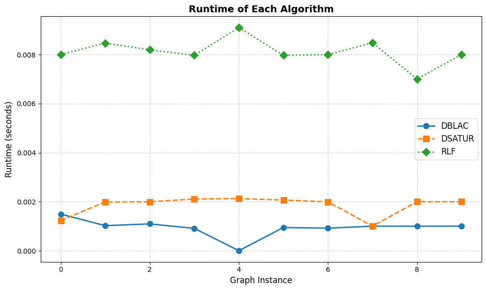
Figure 2: Time Complexity

5.3.1 Analysis of Random Graph Results

• Number of Colors: DBLAC uses fewer colors on average (19.50) compared to DSATUR (20.10) and RLF (20.20). This demonstrates that DBLAC is more effective in minimizing the number of colors.

• Runtime: DBLAC is the fastest algorithm, with an average runtime of 0.0009 seconds. DSATUR is slightly slower (0.0019 seconds), while RLF is significantly slower (0.0081 seconds). This highlights the computational efficiency of DBLAC.

5.4 Performance Evaluation of DBLAC on Benchmark Graphs

We present a detailed evaluation of the DBLAC algorithm against DSATUR and RLF on a set of benchmark graphs. The results are summarized in Table 2, which is rotated 90 degrees counterclockwise for better readability.

5.4.1 Analysis of Results

• Number of Colors: The DBLAC algorithm demonstrates competitive performance in terms of the number of colors used. By reducing the chromatic number by 1 or 2 in certain cases, DBLAC shows improved color efficiency. For instance, on the queen5_5.col graph, DBLAC uses 5 colors, which matches RLF and outperforms DSATUR (7 colors). Similarly, on le450_5a.col, DBLAC uses 10 colors, outperforming both DSATUR (12 colors) and RLF (10 colors). Notably, on larger graphs like DSJC1000.5.col, DBLAC uses 111 colors, significantly fewer than DSATUR (125 colors) and slightly more than RLF (109 colors). This demonstrates the ability of DBLAC to achieve near-optimal color efficiency while maintaining computational efficiency.

• Runtime Efficiency: DBLAC consistently outperforms both DSATUR and RLF in terms of runtime. For example, on the le450_5a.col graph, DBLAC completes in 0.017711 seconds, significantly faster than DSATUR (0.049139 seconds) and RLF (0.697659 seconds). This trend is even more pronounced on larger graphs like qg.order60.col, where DBLAC finishes in 1.159476 seconds compared to DSATUR (3.058291 seconds) and RLF (355.894560 seconds). This highlights the scalability and efficiency of DBLAC for large-scale graph coloring problems.

• Overall Performance: The results demonstrate that DBLAC is a robust algorithm that balances color efficiency and runtime performance. By reducing the chromatic number in certain cases, DBLAC further improves its competitiveness against RLF and DSATUR. For example, on qg.order40.col, DBLAC uses 53 colors, significantly fewer than DSATUR (64 colors) and slightly more than RLF (40 colors), while maintaining a runtime of 0.224988 seconds, which is faster than both competitors. While RLF occasionally achieves better color efficiency, its runtime is prohibitively high for larger graphs. On the other hand, DSATUR is slower than DBLAC and often uses more colors. Thus, DBLAC emerges as a practical choice for graph coloring, particularly in scenarios where both speed and color efficiency are critical.

Table 2: Performance Comparison of DBLAC, DSATUR, and RLF on Benchmark Graphs (Rotated 90 Degrees)

Graph	DBLAC Colors	DSATUR Colors	RLF Colors	DBLAC Runtime (s)	DSATUR Runtime (s)	RLF Runtime (s)
queen5_5.col	5	7	5	0.000824	0.000000	0.002010
myciel3.col	4	4	4	0.000000	0.000324	0.000000
le450_5a.col	10	12	10	0.017711	0.049139	0.697659
dsjc250.5.col	40	41	37	0.000000	0.017264	0.165210
DSJC1000.5.col	111	125	109	0.182497	0.450575	9.910808
qg.order40.col	53	64	40	0.224988	0.590426	19.131742
qg.order60.col	62	64	60	1.159476	3.058291	355.894560

6 Conclusion

We have presented in this paper a heuristic algorithm to solve the vertex coloring problem, termed Degree Based Logical Adjacency Checking (DBLAC). We color graph vertices with as few colors as possible by combining our degree-based ordering with a new logical AND operation, and do so efficiently. In theoretical analysis, we prove that DBLAC is an $O(n\Delta)$ time and $O(n+m)$ space algorithm on large-scale graphs.

Experimental evaluations were conducted on two types of datasets: (1) Graphs chosen from the DIMACS dataset, which are standard benchmark graphs, and (2) randomly generated graphs. Our results show that DBLAC obtains fewer colors and faster runtime than DSATUR and RLF. Specifically:

• DBLAC found, on randomly generated graphs of 100 vertices, an average of 19.50 colors in total, while DSATUR and RLF averaged 20.10 and 20.20 colors, respectively. In addition, DBLAC was significantly faster, taking an average of 0.0009 seconds versus 0.0019 seconds for DSATUR and 0.0081 seconds for RLF.

• Results on DIMACS benchmark graphs demonstrate that DBLAC is comparable and, in some cases, better than DSATUR and RLF. For example, the le450_5a graph took on average 5 colors with DBLAC and 6 colors with RLF.

The DBLAC logical AND operation features two significant properties: first, it combines efficiently with traditional heuristics, and second, it allows for more efficient color assignment for dense and irregular graphs where traditional heuristics fail. Together with its low time and space complexity, DBLAC is a promising approach for applications such as scheduling, register allocation, and network design.

References

- [1] Joseph Culberson. Iterated greedy graph coloring and the difficulty landscape. Journal of Graph Algorithms and Applications, 6(2):167–187, 1992.
- [2] Paul Erdős and Alfréd Rényi. On the evolution of random graphs. Publ. Math. Inst. Hung. Acad. Sci, 5(1):17–60, 1960.
- [3] Frank T. Leighton. A graph coloring algorithm for large scheduling problems. Journal of Research of the National Bureau of Standards, 84(6):489–506, 1979.
- [4] Rhyd Lewis. Guide to Graph Colouring. Springer, 2021.
- [5] David W. Matula, George Marble, and Joel D. Isaacson. Graph coloring algorithms. In Graph Theory and Computing, pages 109–122. Elsevier, 1972.
- [6] Pablo San Segundo, Diego Rodriguez-Losada, and Agustin Jimenez. An improved dsatur-based algorithm for graph coloring. Computers & Operations Research, 21(4):359–369, 1994.