Survey of Radiative, Two-Temperature Magnetically Arrested Simulations of the Black Hole M87* I: Turbulent Electron Heating

Abstract

We present a set of eleven two-temperature, radiative, general relativistic magnetohydrodynamic (2TGRRMHD) simulations of the black hole M87* in the magnetically arrested (MAD) state, surveying different values of the black hole spin $a_{*}$. Our 3D simulations self-consistently evolve the temperatures of separate electron and ion populations under the effects of adiabatic compression/expansion, viscous heating, Coulomb coupling, and synchrotron, bremsstrahlung, and inverse Compton radiation. We adopt a sub-grid heating prescription from gyrokinetic simulations of plasma turbulence. Our simulations have accretion rates $\dot{M}=(0.5-1.5)\times 10^{-6}\dot{M}_{\rm Edd}$ and radiative efficiencies $\epsilon_{\rm rad}=3-35\%$. We compare our simulations to a fiducial set of otherwise identical single-fluid GRMHD simulations and find no significant changes in the outflow efficiency or black hole spindown parameter. Our simulations produce an effective adiabatic index for the two-temperature plasma of $\Gamma_{\rm gas}\approx 1.55$, larger than the $\Gamma_{\rm gas}=13/9$ value often adopted in single-fluid GRMHD simulations. We find moderate ion-to-electron temperature ratios in the 230 GHz emitting region of $R=T_{\rm i}/T_{\rm e}{\approx}5$. While total intensity 230 GHz images from our simulations are consistent with Event Horizon Telescope (EHT) results, our images have significantly more beam-scale linear polarization ($\langle|m|\rangle\approx 30\%$) than is observed in EHT images of M87* ($\langle|m|\rangle<10\%$). We find a trend of the average linear polarization pitch angle $\angle\beta_{2}$ with black hole spin consistent with what is seen in single-fluid GRMHD simulations, and we provide a simple fitting function for $\angle\beta_{2}(a_{*})$ motivated by the wind-up of magnetic field lines by black hole spin in the Blandford-Znajek mechanism.

1 Introduction

Most supermassive black holes are surrounded by hot, low-luminosity plasma accretion flows (Greene & Ho, 2007; Ho, 2008). Emission from these low-luminosity accretion flows is predominantly produced by synchrotron radiation from relativistic electrons at millimetre wavelengths (Ichimaru, 1977; Narayan & Yi, 1994; Yuan & Narayan, 2014). The Event Horizon Telescope (EHT) Very-Long-Baseline Interferometry (VLBI) experiment has resolved millimetre-wavelength synchrotron images on scales of the event horizon $r\mathrel{\raise 1.29167pt\hbox{$<$\kern-7.5pt\lower 4.30554pt\hbox{$\sim$}}}5\,r_{\rm g}=5\,GM/c^{2}$ in the nearby low-luminosity AGN M87* (Event Horizon Telescope Collaboration et al., 2019a) and the Galactic Centre black hole Sgr A* (Event Horizon Telescope Collaboration et al., 2022a).

The elliptical galaxy M87 displays a prominent extragalactic jet (Curtis, 1918) extending from the central supermassive black hole (Hada et al., 2011) to kiloparsec distances, with emission across the electromagnetic spectrum (Event Horizon Telescope Collaboration et al., 2024a). Extragalactic jets like that in M87 are widely believed to be powered by the central black hole’s spin energy, extracted by magnetic fields threading the event horizon (Blandford & Znajek, 1977), though an alternative power source from rotational energy in the accretion disc (Blandford & Payne, 1982) cannot yet be ruled out. Millimetre-wavelength VLBI images of M87* in full polarization map out the geometry and strength of the magnetic field just outside the event horizon and have the potential to directly probe the energy source of M87’s extragalactic jet (Chael et al., 2023; Johnson et al., 2023; Event Horizon Telescope Collaboration, 2024).

General Relativistic Magnetohydrodynamic (GRMHD) simulations are an essential tool for understanding the properties of hot accretion flows and jets around supermassive black holes (e.g. Komissarov, 1999; Gammie et al., 2003). Using general relativistic ray-tracing and synchrotron radiation transfer codes (e.g. Dexter, 2016; Mościbrodzka & Gammie, 2018; Prather et al., 2023), it is possible to generate simulated horizon-scale millimetre images of M87*, Sgr A*, and other sources (e.g. Zhang et al., 2024) for direct comparison to VLBI observations. An extensive comparison of simulated images from GRMHD simulations to polarized EHT observations indicates that M87* (Event Horizon Telescope Collaboration et al., 2021b, 2023) and Sgr A* (Event Horizon Telescope Collaboration et al., 2024b) are likely in the magnetically arrested (MAD) state of black hole accretion, where the magnetic field near the black hole is largely ordered and dynamically important (Narayan et al., 2003; Tchekhovskoy et al., 2011).

The hot accretion flows around M87* and Sgr A* are so low density that electrons and ions are not in thermal equilibrium (Shapiro et al., 1976; Rees et al., 1982). Single-fluid GRMHD simulations assume equilibrium, and thus do not provide any direct constraints on the temperature of the electrons that produce the observed emission. In practice when producing simulated GRMHD images, the ion-to-electron temperature ratio is set with an ad hoc prescription in post-processing (e.g. Shcherbakov et al., 2012; Dexter et al., 2012); the most common prescription (Mościbrodzka et al., 2016) used to interpret EHT images sets the temperature ratio $R=T_{\rm i}/T_{\rm e}$ as a two-parameter function of the local ratio of the gas to magnetic pressure $\beta_{\rm gas}=p_{\rm gas}/p_{\rm mag}$. A lack of direct constraints on the electron temperature $T_{\rm e}$ from simulations is a limiting source of theoretical uncertainty in interpreting EHT observations.

Ressler et al. (2015) introduced a new method to constrain $T_{\rm e}$ directly in black hole accretion simulations by extending the equations of GRMHD to include the thermodynamic evolution of separate electron and ion species. For M87*, the moderately high radiative efficiency (Event Horizon Telescope Collaboration et al., 2021b) means that radiative cooling is significant in determining $T_{\rm i}/T_{\rm e}$, so it is important to extend the two-temperature simulations further to include radiative feedback (Sądowski et al., 2017; Liska et al., 2024). Two-temperature simulations of Sgr A* (Ressler et al., 2017; Chael et al., 2018; Dexter et al., 2020; Yoon et al., 2020; Salas et al., 2024; Mościbrodzka, 2024) and M87* (Ryan et al., 2018; Chael et al., 2019; Yao et al., 2021) have successfully reproduced horizon-scale total intensity images consistent with post-processing models and EHT results.

While two-temperature, radiative GRMHD (2TGRRMHD) simulations have the potential to directly constrain the temperature of the electrons emitting the observed near-horizon radiation, these simulations have drawbacks when compared to the standard single-fluid GRMHD approach. Because radiative coupling is usually handled implicitly (Sądowski et al., 2017; Liska et al., 2022), 2TGRRMHD simulations are significantly more computationally expensive than standard GRMHD evolution. Furthermore, adding radiation feedback breaks the scale-freedom of the ideal GRMHD equations; 2TGRRMHD simulations cannot be re-scaled freely in post-processing to match sources with different black hole masses and accretion rates. Finally, while the physics of electron cooling is well constrained, it is still uncertain exactly how electrons are heated and accelerated on microscopic scales around black holes. 2TGRRMHD parameterize this uncertainty in the choice of sub-grid electron heating function, $\delta_{\rm e}$, which determines how much of the dissipated energy heats electrons as a function of local plasma parameters. Two main families of models for $\delta_{\rm e}$ have been studied in 2TGRRMHD simulations, with electron heating originating from a turbulent cascade truncated by Landau damping (Howes, 2010; Kawazura et al., 2019) or from sub-grid magnetic reconnection with or without a substantial guide field (Rowan et al., 2017, 2019).

Because of the additional computational expense, single-source limitations, and uncertainty in the underlying electron heating mechanism, relatively few two-temperature GRMHD simulations of M87* have been conducted. In particular, there has not yet been an attempt to produce 2TGRRMHD versions of the simulation image “libraries” spanning different values of the black hole spin $a_{*}$ and electron temperature parameters that are the bedrock tool of analysis of polarized EHT observations with single-fluid GRMHD simulations (Event Horizon Telescope Collaboration et al., 2019b, 2021b, 2022b; Event Horizon Telescope Collaboration et al., 2024b). In this paper, we begin a systematic series of investigations of a survey of 2TGRRMHD simulations of magnetically arrested models of M87*. We present a survey of 2TGRRMHD simulations of MAD accretion on a $M=6.5\times 10^{9}M_{\odot}$ black hole with the accretion rate tuned to produce M87*’s 230 GHz observed flux density $F_{230}=0.5$ Jy (Event Horizon Telescope Collaboration et al., 2019a, 2024a). We compare the properties of our 2TGRRMHD simulations to fiducial single-fluid GRMHD simulations run with the same code and parameters, investigate the resulting distributions of electron and ion temperatures, and inspect the features of the resulting simulated 230 GHz images in total intensity and polarization across different values of black hole spin. In this paper, we explore only one choice of the electron heating function $\delta_{\rm e}$, the Kawazura et al. (2019) (K19) model of heating from plasma turbulence. We will compare the simulations presented here with analogous simulations conducted using the Rowan et al. (2019) (R19) prescription for heating from magnetic reconnection in a future work.

The paper is organized as follows. In section 2 we review the equations and method of 2TGRRMHD evolution in the code KORAL (Sądowski et al., 2013). In section 3 we define the parameters of our simulation suite. In section 4 we investigate the results of our 2TGRRMHD simulations, comparing them across different values of the black hole spin and their non-radiative counterparts; we also investigate their resulting 230 GRMHD images and compare them to EHT observations of M87*. We discuss and conclude in section 5.

2 Two-Temperature, Radiative GRMHD Equations

2.1 Units

Except where otherwise noted, we use units where $G=c=1$. Length and time are measured relative to the gravitational length-scale $r_{\rm g}=GM/c^{2}$ and time-scale $t_{\rm g}=GM/c^{3}$, where $M$ is the black hole mass. The black hole accretion rate is measured relative to the Eddington accretion rate $\dot{M}_{\mathrm{Edd}}=L_{\mathrm{Edd}}/\eta_{\rm Edd}c^{2}=4\pi\,GMm_{\rm p}/\eta_{\rm Edd}c\sigma_{\rm T}$, where $m_{\rm p}$ is the proton mass, $\sigma_{\rm T}$ is the Thomson cross section, and we adopt an efficiency parameter $\eta_{\rm Edd}=0.1$. We frequently refer to the dimensionless black hole spin parameter $a_{*}=J/M^{2}$, where $J$ is the black hole’s angular momentum.

For our simulations targeted at M87*, we adopt a black hole mass $M=6.5\times 10^{9}M_{\odot}$ and we assume the distance to M87* is $D=16.8$ Mpc (Event Horizon Telescope Collaboration et al., 2019c). For this choice of black hole mass, $r_{\rm g}=9.6\times 10^{14}\,\mathrm{cm}=64\,\mathrm{AU}$, $t_{\rm g}=3.2\times 10^{4}\,\mathrm{s}=8.9\,\mathrm{hr}$, and $\dot{M}_{\rm Edd}=9.1\times 10^{27}\,\mathrm{g\,s}^{-1}=144.3\,M_{\rm\odot}\,\mathrm{yr}^{-1}$. The projected size of the gravitational radius is $\theta_{\rm g}=r_{\rm g}/D=3.82\,\mu$as.

2.2 Equations

Here we review the equations of two-temperature, radiative GRMHD used in the code KORAL (Sądowski et al., 2017). The code evolves two fluids representing electrons ($\mathrm{e}$) and ions ($\mathrm{i}$) in a fully-ionized plasma.

The number densities of electrons and ions are related to the fluid rest-mass density $\rho$ by $n_{\rm e,i}=\rho/\left(\mu_{\rm e,i}m_{\rm p}\right)$, where $m_{\rm p}$ is the proton mass and $\mu_{\rm e,i}$ is the electron (ion) mean molecular mass. In this work, we assume the gas is fully ionized hydrogen, so $\mu_{\rm e}=\mu_{\rm i}=1$. The electron and ion pressures $p_{\rm e,i}$ are related to their respective temperatures $T_{\rm e,i}$ by the ideal gas law, $p_{\rm e,i}=n_{\rm e,i}k_{\rm B}T_{\rm e,i}$. The electron/ion internal energies are then given by an equation of state:

$$u_{\rm e,i} =\frac{p_{\rm e,i}}{\Gamma_{\rm e,i}(\Theta_{\rm e,i})-1},$$ (1)

where the dimensionless temperature for electrons and ions is $\Theta_{\rm e,i}=k_{\rm B}T_{\rm e,i}/m_{\rm e,i}c^{2}$, where $m_{\rm e}$ is the electron mass and $m_{\rm i}=\mu_{\rm i}m_{\rm p}$ is the mean ion mass. We assume both species are in a relativistic Maxwell-Jüttner distribution; $\Gamma(\Theta)$ is a temperature-dependent adiabatic index that transitions from $\Gamma=5/3$ for a non-relativistic fluid, $\Theta\ll 1$, to $\Gamma=4/3$ for a relativistic fluid, $\Theta\gg 1$. The form of $\Gamma(\Theta)$ we use is given in Sądowski et al. (2017), Equation A14.

We assume the electron and ion fluids combine to form an effective single fluid with total pressure $p_{\rm gas}=p_{\rm e}+p_{\rm i}$ and energy density $u_{\rm gas}=u_{\rm e}+u_{\rm i}$. The effective combined gas temperature $T_{\rm gas}$ and adiabatic index $\Gamma_{\rm gas}$ are then

$$T_{\mathrm{gas}} =\mu_{\rm gas}\left(\frac{T_{\mathrm{i}}}{\mu_{\rm i}}+\frac{T_{\mathrm{e}}}{\mu_{\rm e}}\right),$$ (2)

$$\Gamma_{\rm gas} =1+\frac{\left(\Gamma_{\mathrm{i}}-1\right)\left(\Gamma_{\mathrm{e}}-1\right)\left(T_{\mathrm{i}}/T_{\mathrm{e}}+\mu_{\rm i}/\mu_{\rm e}\right)}{\left(T_{\mathrm{i}}/T_{\mathrm{e}}\right)\left(\Gamma_{\mathrm{e}}-1\right)+\left(\mu_{\rm i}/\mu_{\rm e}\right)\left(\Gamma_{\mathrm{i}}-1\right)},$$ (3)

where the effective mean molecular mass for the combined two-fluid plasma is $\mu^{-1}_{\rm gas}=\mu_{\rm e}^{-1}+\mu_{\rm i}^{-1}$; $\mu_{\rm gas}=1/2$ in our simulations assuming pure Hydrogen.

The combined electron-ion fluid and electromagnetic field together make up the MHD stress-energy tensor $T^{\mu}_{\;\;\nu}$;

$$T^{\mu}_{\;\;\nu} =\left(\rho+u_{\rm gas}+p_{\rm gas}+b^{2}\right)u^{\mu}u_{\nu}+\left(p_{\rm gas}+\frac{1}{2}b^{2}\right)\delta^{\mu}_{\;\;\;\nu}-b^{\mu}b_{\nu}.$$ (4)

The fluid four-velocity is $u^{\mu}$ and the fluid-frame magnetic field vector is $b^{\mu}=u_{\nu}\star F^{\nu\mu}$, where $\star F^{\nu\mu}$ is the dual of the electromagnetic field Faraday tensor $F^{\nu\mu}$. We take the ideal MHD limit, where the fluid is assumed to be infinitely conductive so that the fluid-frame electric field vanishes, $e^{\mu}=u_{\nu}F^{\mu\nu}=0$. In the ideal MHD limit, $b^{\mu}$ can be computed from $u^{\mu}$ and the “lab-frame” magnetic field $B^{i}=\star F^{i0}$ in the standard way (e.g. Gammie et al., 2003).

In addition to the plasma and magnetic field, we also evolve a radiation field coupled to the plasma using the M1 approximation, where we assume there always exists a timelike frame $u^{\mu}_{\rm R}$ where the radiation stress-energy $R^{\mu}_{\;\;\nu}$ is isotropic. The radiation field stress-energy tensor in the M1 approximation is

$$R^{\mu}_{\;\;\nu} =\frac{4}{3}\bar{E}u^{\mu}_{\rm R}u^{\vphantom{\mu}}_{\rm R\,\nu}+\frac{1}{3}\bar{E}\delta^{\mu}_{\;\;\nu},$$ (5)

where $\bar{E}$ is the radiation energy density in the frame co-moving with $u^{\mu}_{\rm R}$. To account for frequency-dependence in emission and absorption processes to first order, KORAL also tracks the photon number density $\bar{n}_{\rm R}$, which provides the mean photon frequency in the fluid frame $\hat{E}/h\hat{n}_{\rm R}$, or equivalently, the effective radiation blackbody temperature $T_{\rm R}$ (Sądowski & Narayan, 2015).

The coupled evolution equations for the two-temperature fluid, the electromagnetic field, and the radiation field are

$$\nabla_{\mu}(\rho u^{\mu}) =0,$$ (6)

$$\nabla_{\mu}\left(T^{\mu\nu}\right) =G_{\nu},$$ (7)

$$\nabla_{\mu}\left(R^{\mu\nu}\right) =-G_{\nu},$$ (8)

$$\nabla_{\mu}\left(\star F^{\mu\nu}\right) =0,$$ (9)

where $G^{\nu}$ is the radiation four-flux, obtained from the emissivities and opacities for the radiation processes considered using the formulae in (Sądowski et al., 2017). In our simulations, we consider radiation from synchrotron, bremsstrahlung, Thomson and Compton scattering processes, though synchrotron emission is the main contribution to $G^{\nu}$ (Salas et al., 2024). The evolution equation for the photon number density is

$$\nabla_{\mu}\left(\bar{n}^{\vphantom{\mu}}_{\rm R}u^{\mu}_{R}\right)=\dot{\bar{n}}_{\rm R},$$ (10)

where $\dot{\bar{n}}_{\rm R}$ is the photon production rate in the radiation frame (see Sądowski & Narayan, 2015; Sądowski et al., 2017).

To evolve the individual energy densities of the electron and ion fluids, we use the first law of thermodynamics for each with appropriate source terms;

$$T_{\mathrm{e}}\nabla_{\mu}\left(n_{\rm e}s_{\mathrm{e}}u^{\mu}\right) =\delta_{\mathrm{e}}q^{\rm v}+q^{\rm C}-\hat{G}^{0},$$ (11)

$$T_{\mathrm{i}}\nabla_{\mu}\left(n_{\rm i}s_{\mathrm{i}}u^{\mu}\right) =(1-\delta_{\mathrm{e}})q^{\rm v}-q^{\rm C}.$$ (12)

In Equation 11 and Equation 12, $s_{\rm e,i}$ is the temperature-dependent entropy per particle of the electron and ion species (see Equation A11 of Sądowski et al. 2017 for the form of $s(n,\Theta)$ that we use), $q^{\rm v}$ is the viscous heating rate, $q^{\rm C}$ is the Coulomb coupling rate (Stepney & Guilbert, 1983), and $\hat{G}^{0}$ is the radiation cooling rate transformed to the fluid frame. The parameter $\delta_{\rm e}$ controls the fraction of the total dissipated energy that goes into electrons.

As in (Sądowski et al., 2017; Chael et al., 2019; Salas et al., 2024), we compute the viscous heating rate $q^{\rm v}$ numerically by first evolving Equation 11 and Equation 12 without source terms and then comparing the sum of the adiabatically evolved electron and ion energy densities to the separately-evolved total fluid energy $u_{\rm gas}$. To determine the electron heating fraction $\delta_{\rm e}$, we adopt the Kawazura et al. (2019) (hereafter K19) prescription from gyrokinetic simulations of plasma turbulence. The Kawazura et al. (2019) heating prescription gives $\delta_{\rm e}$ as a function of the local electron-to-ion temperature ratio and plasma-beta:

$$\frac{Q_{\rm i}}{Q_{\rm e}} =\frac{35}{\left(\beta_{\rm i}/15\right)^{-1.4}e^{-0.1T_{\rm e}/T_{\rm i}}},$$ (13)

$$\delta_{\rm e} =\frac{1}{1+Q_{\rm i}/Q_{\rm e}},$$ (14)

where the plasma-beta parameter for the ions $\beta_{\rm i}$ is the ratio of the ion to magnetic pressure in the fluid frame:

$$\beta_{\rm i}=\frac{p_{\rm i}}{p_{\rm mag}}=\frac{2n_{\rm i}k_{\rm B}T_{\rm i}}{b^{2}}.$$ (15)

Note that $\beta_{\rm i}$ defined in Equation 15 is the plasma-beta parameter defined relative to the ion temperature; we also make use of a similarly-defined electron beta $\beta_{\rm e}=p_{\rm e}/p_{\rm mag}$ and the standard plasma-beta for the combined electron-ion gas, $\beta_{\rm gas}=p_{\rm gas}/p_{\rm mag}=\beta_{\rm e}+\beta_{\rm i}$. We also often make use of the plasma magnetization parameter, which represents the ratio of the magnetic energy density to the ion rest mass energy density:

$$\sigma_{\rm i}=\frac{b^{2}}{n_{\rm i}m_{\rm i}c^{2}}.$$ (16)

3 Simulations

We ran a total of 11 radiative two-temperature GRMHD simulations of M87* and 11 corresponding benchmark ideal single-fluid simulations in the code KORAL (Sądowski et al., 2013; Sądowski et al., 2017). All of our simulations were conducted in the magnetically arrested (MAD) state, and we span a range of black hole spins $a_{*}\in\{\pm 0.9,\pm 0.7,\pm 0.5,\pm.0.3,\pm 0.1,0\}$. We list the simulations considered here in Table 1.

Model	$a_{*}$	$B$-field	Radiation	Electron Heating	$N_{r}\times N_{\theta}\times N_{\phi}$	$r_{\rm min}/r_{\rm g}$	$r_{\rm max}/r_{\rm g}$	$\langle\dot{M}\rangle/10^{-7}\dot{M}_{\rm Edd}$	$\langle\phi_{\rm BH}\rangle$	$\langle\eta\rangle$	$\langle s\rangle$	$\langle\epsilon_{\rm rad}\rangle/10^{-2}$
ap9	0.9	MAD	No	-	$288\times 192\times 144$	1.18	$10^{4}$	9.8	46.7	1.2	-8.1	-
ap7	0.7	MAD	No	-	$288\times 192\times 144$	1.41	$10^{4}$	13.9	60.5	0.9	-9.4	-
ap5	0.5	MAD	No	-	$288\times 192\times 144$	1.54	$10^{4}$	20.4	59.0	0.4	-6.0	-
ap3	0.3	MAD	No	-	$288\times 192\times 144$	1.61	$10^{4}$	24.6	60.7	0.2	-3.7	-
ap1	0.1	MAD	No	-	$288\times 192\times 144$	1.65	$10^{4}$	31.7	53.4	0.1	-0.6	-
ap0	0.0	MAD	No	-	$288\times 192\times 144$	1.65	$10^{4}$	30.8	57.1	0.0	0.6	-
am1	-0.1	MAD	No	-	$288\times 192\times 144$	1.65	$10^{4}$	28.8	52.2	0.1	1.9	-
am3	-0.3	MAD	No	-	$288\times 192\times 144$	1.61	$10^{4}$	26.3	45.8	0.1	3.6	-
am5	-0.5	MAD	No	-	$288\times 192\times 144$	1.54	$10^{4}$	29.1	36.8	0.1	4.4	-
am7	-0.7	MAD	No	-	$288\times 192\times 144$	1.41	$10^{4}$	15.9	28.8	0.2	4.7	-
am9	-0.9	MAD	No	-	$288\times 192\times 144$	1.18	$10^{4}$	16.3	23.4	0.3	5.1	-
ap9_radk	0.9	MAD	Yes	K19	$288\times 192\times 144$	1.18	$10^{4}$	5.7	43.6	1.2	-6.8	32.9
ap7_radk	0.7	MAD	Yes	K19	$288\times 192\times 144$	1.41	$10^{4}$	8.1	57.8	0.9	-8.3	24.3
ap5_radk	0.5	MAD	Yes	K19	$288\times 192\times 144$	1.54	$10^{4}$	8.9	57.5	0.4	-5.7	12.6
ap3_radk	0.3	MAD	Yes	K19	$288\times 192\times 144$	1.61	$10^{4}$	10.0	63.1	0.2	-4.1	10.0
ap1_radk	0.1	MAD	Yes	K19	$288\times 192\times 144$	1.65	$10^{4}$	12.5	57.1	0.1	-0.9	4.6
ap0_radk	0.0	MAD	Yes	K19	$288\times 192\times 144$	1.65	$10^{4}$	11.3	54.2	0.1	0.5	3.6
am1_radk	-0.1	MAD	Yes	K19	$288\times 192\times 144$	1.65	$10^{4}$	14.8	50.2	0.1	1.6	4.4
am3_radk	-0.3	MAD	Yes	K19	$288\times 192\times 144$	1.61	$10^{4}$	15.5	45.1	0.1	3.1	4.3
am5_radk	-0.5	MAD	Yes	K19	$288\times 192\times 144$	1.54	$10^{4}$	13.3	37.5	0.1	3.7	5.4
am7_radk	-0.7	MAD	Yes	K19	$288\times 192\times 144$	1.41	$10^{4}$	9.2	36.7	0.2	4.8	9.3
am9_radk	-0.9	MAD	Yes	K19	$288\times 192\times 144$	1.18	$10^{4}$	13.3	27.2	0.3	4.6	11.4

Table 1: Summary of 3D MAD simulations presented in this work. For each simulation we report the spin $a_{*}$, the magnetic field configuration (all simulations are in the MAD state), whether the simulation includes radiation feedback, and the electron heating function (we use only the Kawazura et al. (2019) function K19 in this work). We also report the simulation resolution and the inner and outermost simulation radii $r_{\rm min},r_{\rm max}$. Over the final $[15000,20000]\,t_{\rm g}$ interval of each simulation we compute the mean mass accretion rate through the horizon $\dot{M}$ (Equation 17) in Eddington units, the normalized horizon magnetic flux $\phi_{\rm BH}$ (Equation 19), the outflow efficiency $\eta$ (Equation 22), the spindown parameter $s$ (Equation 23), and for the radiative simulations, the radiative efficiency $\epsilon_{\rm rad}$ (Equation 26). The values of $\dot{M}/\dot{M}_{\rm Edd}$ for the non-radiative models reported here correspond to a density scaling used to match a median 230 GHz flux density $F_{230}=0.5$ Jy for each simulation using a $R_{\rm low}=10,R_{\rm high}=40$ Mościbrodzka et al. (2016) electron temperature model.

3.1 Numerical Implementation

We concentrate resolution in the jet region close to the polar axis and the disc region near the equator by transforming standard Kerr-Schild spatial coordinates $(r,\theta,\phi)$ to the “jetcoords” coordinate system $(x_{1},x_{2},x_{3})$ introduced in Ressler et al. (2017) and used in Narayan et al. (2022). Each simulation has a resolution of $288,192,144$ in the uniform grid of code coordinates $(x_{1},x_{2},x_{3})$. The radial coordinate $x_{1}$ is logarithmically spaced from $r_{\rm min}=0.825r_{+}$ to $r_{\rm max}=10^{4}\,r_{\rm g}$, where $r_{+}$ is the radius of the event horizon. The simulation grid is uniform in $x_{3}=\phi$. The polar angle $\theta$ is a function of both $x_{1}$ and $x_{2}$; we use the same parameters for this transformation as Narayan et al. (2022), except that the minimum value of the $x_{2}$ coordinate here is $x_{2,\mathrm{min}}=10^{-3}$.

We initialized the single-fluid simulations with a Fishbone & Moncrief (1976) equilibrium torus with a constant inner radius $r_{\rm in}=20\,r_{\rm g}$. Because the outer edge of the Fishbone & Moncrief (1976) torus is highly sensitive to the combination of black hole spin, inner edge $r_{\rm in}$, and radius of maximum pressure $r_{p,\mathrm{max}},$ we follow Narayan et al. (2022) and choose a spin-dependent pressure maximum radius in the range $r_{p,\mathrm{max}}\sim 40-42\,r_{\rm g}$ such that our initial tori all have outer edges inside the simulation domain. To evolve the system to the MAD state, we initialized the torus with a coherent loop of poloidal magnetic field centred exactly as in Narayan et al. (2022). The magnetic field strength in the disc was normalized so that the ratio of the maximum gas pressure to maximum magnetic pressure in the torus $p_{\rm gas,max}/p_{\rm mag,max}=100$.

Like most GRMHD codes (e.g. Gammie et al., 2003), KORAL solves the GRMHD equations in a finite-volume scheme. KORAL reconstructs primitive quantities at cell walls using the second-order piecewise parabolic method (PPM) and uses the local Lax-Friedrichs method to evaluate fluxes. The coupling $G^{\nu}$ between the fluid and radiation is handled implicitly, and the time evolution is performed with a second-order Implicit-Explicit (IMEX) scheme. The magnetic field evolution is constrained to conserve the initially zero divergence with the constrained transport algorithm of Tóth (2000). Our simulations use outflowing boundary conditions at the inner boundary $r_{\rm min}$ inside the event horizon and at $r_{\rm max}$. The azimuthal boundary is periodic. We use reflecting boundary conditions at the polar axis, with a modification to the $x_{2}$-component of the plasma (or radiation-frame) velocity in the inner two cells such that this component goes to zero at the pole.

We first evolved the 11 single-fluid GRMHD simulations from Kerr-Schild time $t=0$ to $t=10^{4}\,t_{\rm g}$. During this initial period, gas in the torus begins to accrete and the magnetic field builds up on the black hole, eventually saturating at a value of the dimensionless magnetic flux (or “MAD parameter”) $\phi_{\rm BH}\approx 50$, where $\phi$ is given by Equation 19. At this point, we initialized the eleven two-temperature, radiative simulations from the already-accreting single-fluid GRMHD data. We ran both the parent single-fluid simulations and the two-temperature simulations from this point to a maximum time $t=2\times 10^{4}\,t_{\rm g}$.

When re-starting the single fluid GRMHD simulations to evolve the 2TGRRMHD equations, we initialize the radiation energy density $\bar{E}=10^{-4}u_{\rm gas}$, and the electron energy density $u_{\rm e}=0.05u_{\rm gas}$, (so $u_{\rm i}=0.95u_{\rm gas}$). Single-fluid GRMHD simulations are scale-free, but radiative simulations require a fixed choice of physical energy density scale. We first scale the density and energy densities so that the average black hole accretion rate in the range $t\in[9000,10000]\,t_{\rm g}$ is $\dot{M}=10^{-6}\dot{M}_{\rm Edd}$, an approximate value for M87* MAD models (Event Horizon Telescope Collaboration et al., 2019b). We then run the simulation for an additional $500\,t_{\rm g}$ so the radiation and two-temperature effects in the innermost accretion flow can reach an approximate steady-state. We then re-scale the simulation density and energy densities a second time so that the median 230 GHz flux density from synchrotron emission in the last $250\,t_{\rm g}$ is $F_{230}=0.5$ Jy Event Horizon Telescope Collaboration et al. (2019a). We finally ran the radiative simulations from this point forward without additional density rescalings during the simulation runtime to the maximum time of $t=2\times 10^{4}\,t_{\rm g}$, but when producing 230 GHz images for comparison to EHT observations we apply a small post-processing density rescaling to account for secular drifts in $F_{230}$ (see subsection 3.2). We save snapshots of each simulation every $10\,t_{\rm g}$.

In our radiative, two-temperature simulations the adiabatic index is adjusted self-consistently in each cell at each time step to reflect the local ion and electron temperatures through Equation 2. In our single-fluid benchmark GRMHD simulations, we use a fixed adiabatic index $\Gamma_{\rm gas}=13/9$ throughout, corresponding to $T_{\rm e}=T_{\rm i}$, $\Gamma_{\rm e}=4/3$, $\Gamma_{\rm i}=5/3$. All of our radiative simulations use the K19 electron heating function Equation 13.

While we have recently added the option for hybrid GRMHD and Force-Free evolution for magnetized accretion flows in KORAL (Chael, 2024), for this simulation suite we use the standard approach of applying density floors in our simulation to ensure numerical stability in highly-magnetized regions. KORAL injects rest mass in the zero-angular observer (ZAMO) frame to enforce a maximum magnetization $\sigma_{\rm i}\leq\sigma_{\rm max}=100$. To ensure numerical stability, KORAL also applies other floors and ceilings on the plasma (and radiation) energy densities, the plasma (and radiation-frame) Lorentz factor, and on the electron and ion temperatures (Sądowski et al., 2017; Porth et al., 2019).

3.2 230 GHz Images

Model	$f_{230}$
ap9_radk	1.27
ap7_radk	0.99
ap5_radk	1.23
ap3_radk	1.23
ap1_radk	1.04
a0_radk	1.08
am1_radk	0.91
am3_radk	0.98
am5_radk	1.02
am7_radk	0.93
am9_radk	0.94

Table 2: Secondary density rescaling factors for radiative simulations.

To simulate EHT observations of M87*, we produce 230 GHZ images from the eleven radiative simulations using the GR radiative transfer code ipole (Mościbrodzka & Gammie, 2018). For each simulation we produce 500 snapshot images in full polarization covering the time range $15000-20000\,t_{\rm gc}$. Following Event Horizon Telescope Collaboration et al. (2019b), we fix the observer inclination of the prograde simulations (including $a_{*}=0$) to $\theta_{\rm o}=163\deg$ and the viewing inclination of the retrograde simulations to $\theta_{\rm o}=17\deg$ (Mertens et al., 2016). We orient the images so the black hole spin faces East (a position angle $\varphi=90\deg$ counter-clockwise from vertical). We exclude emission from highly magnetized regions with $\sigma_{\rm i}\geq\sigma_{\rm cut}=25$. The field of view of our images is $150\,\mu$as ($\approx\,39\theta_{\rm g}$), and we use a pixel size of $0.3\,\mu$as.

In its 2017 and 2018 observations of M87*, the EHT constrained the 230 GHz compact flux density on horizon scales to be $F_{230}\approx 0.5$ Jy (Event Horizon Telescope Collaboration et al., 2019a, 2024a). As a result, GRMHD simulations of M87* are typically scaled so that the median 230 GHz flux density over some time period matches the observed $0.5$ Jy value. This presents no problem for scale-free pure GRMHD simulations, but introducing radiation fixes a physical density scale which in principle should not be adjusted at all in post-processing. Our radiative simulations were rescaled to achieve $F_{230}\approx 0.5$ Jy at $t=10500\,t_{\rm g}$, but the simulations do not maintain exactly the same median 230 GHz flux density over a wide time window due to secular drifts in the accretion rate and other quantities. In order to provide a direct comparison across the simulations that is consistent with standard practice in the field, the results shown here apply a second small density rescaling to the simulations in post-processing, chosen such that the median $F_{230}=0.5$ Jy in the window $15000-20000\,t_{\rm g}$. The applied post-processing rescaling factor $f_{\rm 230}$ for each simulation is reported in Table 2. Most of the simulations have their density (and internal energy density, magnetic energy density, and radiation energy density) scaled by a factor $<10\%$, with a maximum adjustment of 27% for simulation ap9_radk. None of the results presented below change qualitatively when comparing results with and without this post-processing density rescaling.

We also generate images from our non-radiative GRMHD simulations for comparison with the radiative simulations. To set the electron temperature in the images from the non-radiative simulations, we use the Mościbrodzka et al. (2016) $R_{\rm high},R_{\rm low}$ prescription that adjusts the ion-to-electron temperature ratio $R=T_{\rm i}/T_{\rm e}$ based on the local $\beta_{\rm gas}$. We explore a variety of $R_{\rm low},R_{\rm high}$ combinations in the range $R_{\rm low}\in\{1,10\},R_{\rm high}\in\{1,10,20,40,80,160\}.$

4 Results

All results presented here are taken from the last $5000\,t_{\rm g}$ of evolution from $t=15000\,t_{\rm g}$ to $t=20000\,t_{\rm g}$.

4.1 Average Fluxes

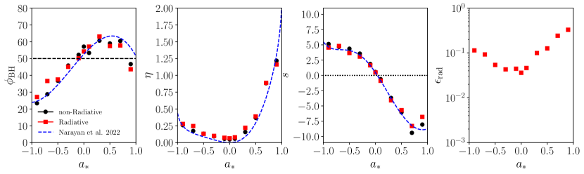
Figure 1: Dimensionless simulation fluxes. The first panel shows the average value of the dimensionless magnetic flux, or “MAD parameter” $\phi_{\rm BH}$ (Equation 19) for all simulations reported in this work as a function of black hole spin $a_{*}$. The second panel shows the outflow efficiency factor $\eta$ (Equation 22) for all simulations, and the third panel plots the spindown parameter $s$ (Equation 23). The final panel plots the bolometric radiative efficiency $\epsilon_{\rm rad}$ (Equation 26) for the radiative simulations. In all panels, results are averaged over the window $t\in\left[15000,20000\right]t_{\rm g}$, and black circles show results from the non-radiative simulations while red squares show results from the radiative, two-temperature simulations. In the first three panels, we plot fitting functions for $\phi_{\rm BH}$, $\eta$, and $s$ derived in Narayan et al. (2022) in dashed blue lines; these correspond to Equations 9, 10, and 15 of Narayan et al. (2022), respectively.

We first compare the average fluxes of mass, magnetic field, energy, and angular momentum for the radiative simulations with their non-radiative counterparts. At each saved snapshot in the range $t\in[15000,20000]t_{\rm g}$ we calculate the black hole accretion rate $\dot{M}$ and magnetic flux through the horizon $\Phi_{\rm BH}$ using the following integrals over the horizon at $r=r_{+}$;

$$\dot{M} =\int_{\theta}\int_{\phi}\left(-\rho u^{r}\right)\sqrt{-g}\;\mathop{}\!\mathrm{d}\phi\mathop{}\!\mathrm{d}\theta,$$ (17)

$$\Phi_{\rm BH} =\int_{\theta}\int_{\phi}\left|B^{r}\right|\sqrt{-g}\;\mathop{}\!\mathrm{d}\phi\mathop{}\!\mathrm{d}\theta,$$ (18)

where $g$ is the metric determinant, and we first convert $u^{\mu}$ and $B^{i}$ from code coordinates to standard Kerr-Schild coordinates. The dimensionless magnetic flux on the horizon, or “MAD parameter” is (Tchekhovskoy et al., 2011):

$$\phi_{\rm BH}=\frac{\sqrt{4\pi}}{2\sqrt{\dot{M}}}\Phi_{\rm BH}.$$ (19)

For accretion discs in the MAD state, the magnetic flux saturates at $\phi_{\rm BH}\approx 50$ (Tchekhovskoy et al., 2011; McKinney et al., 2012), though the precise value is spin- and initial-condition-dependent (Tchekhovskoy & McKinney, 2012; Narayan et al., 2022).

In Table 1, we report the mean values of $\phi_{\rm BH}$ for each simulation over the range $t\in[15000,20000]t_{\rm g}$, and we plot the mean $\phi_{\rm BH}$ as a function of $a_{*}$ in the first panel of Figure 1. We find that the radiative and non-radiative simulations show a similar trend of $\phi_{\rm BH}$ with black hole spin; retrograde simulations have lower $\phi_{\rm BH}$ values which increase as $a_{*}\rightarrow 0$; $\phi_{\rm BH}$ reaches a maximum of $\phi_{\rm BH}\approx 60$ around $a_{*}\approx 0.3-0.5$ before declining again at large positive spin values. This trend is consistent with what is observed in Narayan et al. (2022) (from much longer ideal GRMHD simulations run from the same initial conditions with the same KORAL code) and Tchekhovskoy & McKinney (2012) (from simulations run with a different code). We show the fitting function for $\phi_{\rm BH}(a_{*})$ derived in Narayan et al. (2022) in the left panel of Figure 1 in the dashed blue line. Our results for both the radiative and non-radiative simulations are approximately consistent with the unadjusted Narayan et al. (2022) fitting function; the addition of radiation to our M87* simulations does not significantly affect the average magnetic flux accumulated on the black hole.

We compute the radial angular momentum flux $\dot{J}$ and the radial energy flux $\dot{E}$ at radius $r=5\,r_{\rm g}$ in order to avoid effects from numerical floors close to the horizon, following Narayan et al. (2022). These are:

$$\dot{J} =\int_{\theta}\int_{\phi}-T^{r}_{\phi}\sqrt{-g}\;\mathop{}\!\mathrm{d}\phi\mathop{}\!\mathrm{d}\theta,$$ (20)

$$\dot{E} =\int_{\theta}\int_{\phi}T^{r}_{t}\sqrt{-g}\;\mathop{}\!\mathrm{d}\phi\mathop{}\!\mathrm{d}\theta.$$ (21)

The ratio $\eta$ of the outflowing energy flux to the accretion rate is

$$\eta=\frac{\dot{M}-\dot{E}}{\dot{M}}.$$ (22)

The parameter $\eta$ represents the efficiency of the energy output by the black hole-accretion system. In spinning MAD simulations, nearly all of the outgoing power is in outward electromagnetic Poynting flux in the jet driven by the Blandford & Znajek (1977) process (McKinney & Gammie, 2004; Tchekhovskoy et al., 2011; McKinney et al., 2012); we thus sometimes refer to $\eta$ as a “jet efficiency,” though Equation 22 makes no distinction between the outflowing power in the jet and slow-moving wind components (Narayan et al., 2022).

The black hole spindown (or spinup) parameter $s$ represents the rate of change $a_{*}$ relative to the black hole accretion rate (Shapiro, 2005; Narayan et al., 2022):

$$s=\frac{da_{*}}{dt}\frac{M}{\dot{M}}=\frac{\dot{J}-2a_{*}\dot{E}}{\dot{M}}.$$ (23)

A value of $s$ that is the same sign as the black hole spin indicates that the accretion disc angular momentum is spinning the black hole up; conversely, if $s$ is the opposite sign to $a_{*}$ either the counter-rotating accretion disc or the jet outflow is spinning the black hole down.

In Table 1, we report the mean values of $\eta$ and $s$ for each simulation over the range $t\in[15000,20000]t_{\rm g}$. We plot $\eta$ and $s$ vs black hole spin in the second and third panels of Figure 1. We find that the trend of $\eta$ and $s$ with spin is virtually unchanged by the addition of radiation and two-temperature physics. For the most rapidly spinning black holes with prograde accretion discs, we find $\eta>100\%$, indicating that the energy flowing out in the BZ jet exceeds the rate of rest-mass energy infall through the horizon; for less rapidly spinning prograde discs and for all retrograde MAD disc-jet systems, the jet efficiency $\eta<100\%$. We confirm that the sixth-order BZ result for $\eta(\phi)$ from Tchekhovskoy et al. (2010) fits our measured efficiencies for both the radiative and non-radiative simulations well. The dashed blue line in the second panel of Figure 1 is the same as in Figure 4 of Narayan et al. (2022), namely

$$\eta(\phi_{\rm BH})=\frac{1}{8\pi}\phi^{2}_{\rm BH}\left[\Omega_{\rm H}^{2}+1.38\Omega_{\rm H}^{4}-0.2\Omega_{\rm H}^{6}\right],$$ (24)

where $\Omega_{\rm H}=a_{*}/2r_{+}$ is the angular frequency of the black hole horizon and we use the same fitting function for $\phi_{\rm BH}(a_{*})$ as Narayan et al. (2022). The agreement between the simulation results for $\eta(a_{*})$ and the BZ prediction given the measured magnetic flux $\phi_{\rm BH}$ suggests that most of the outflowing energy is extracted from the BH as Poynting flux in the Blandford & Znajek (1977) process.

Our results for the spindown parameter $s(a_{*})$ in the third panel of Figure 1 also show few differences between the radiative and non-radiative simulations, and both match the previous fitting function derived in Narayan et al. (2022) (blue dashed line). As in that previous work, we find that for all simulations with non-zero spin the spindown parameter $s$ has the opposite sign to $a_{*}$, suggesting that the black hole jet is extracting angular momentum from the black hole more efficiently than it can be supplied by prograde accretion. Thus, jets from magnetically arrested black holes tend to drive the spin to zero if the black hole remains in the magnetically arrested state (Narayan et al., 2022; Ricarte et al., 2023).

For the radiative simulations, we also compute the bolometric luminosity $\dot{L}$:

$$L_{\rm bol} =\int_{\theta}\int_{\phi}-R^{r}_{t}\sqrt{-g}\;\mathop{}\!\mathrm{d}\phi\mathop{}\!\mathrm{d}\theta.$$ (25)

We compute the bolometric luminosity $\dot{L}$ at a larger radius $r=100\,r_{\rm g}$ than we use in computing $\dot{E}$ and $\dot{J}$ in order to account for radiation produced throughout the inner disk and jet regions. The radiative efficiency $\epsilon_{\rm rad}$ is then the ratio of the bolometric luminosity computed at $r=100\,r_{\rm g}$ to the accretion rate at $r=r_{+}$:

$$\epsilon_{\rm rad}=\frac{L_{\rm bol}}{\dot{M}}.$$ (26)

In Table 1, we report average values of $\epsilon_{\rm rad}$, and we plot $\epsilon_{\rm rad}$ against black hole spin in the rightmost panel of Figure 1. The radiative efficiencies in all of our M87* MAD simulations range from 3-35%, in the range consistent with the results from the survey of non-radiative MAD simulations in Event Horizon Telescope Collaboration et al. (2021b). We find that the radiative efficiency increases with both prograde and retrograde spin, though the rapidly spinning prograde models have higher values of $\epsilon_{\rm rad}$ than the rapidly spinning retrograde models.

4.2 Disc Profiles

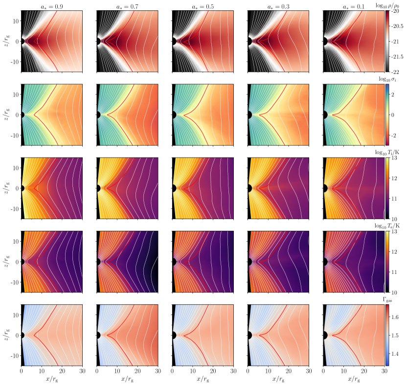
Figure 2: Poloidal profiles of prograde radiative simulations. From left to right, we plot poloidal profiles of the time- and azimuth-averaged quantities from the prograde radiative simulations ap9_radk, ap7_radk, ap5_radk, ap3_radk, and ap1_radk. From top to bottom, we plot the averaged rest mass density $\rho/\rho_{0}$ (where $\rho_{0}=1$ g cm^-3), the magnetization $\sigma_{i}$, ion temperature $T_{\rm i}$, electron temperature $T_{\rm e}$, and adiabatic index $\Gamma_{\rm gas}$. All quantities were averaged over $2\pi$ in azimuth and over the final $5000\,t_{\rm g}$ of simulation runtime. Magenta contours indicate $\sigma_{\rm i}=1$; white contours show surfaces of constant azimuthal vector potential $A_{\phi}$ (Equation 27).

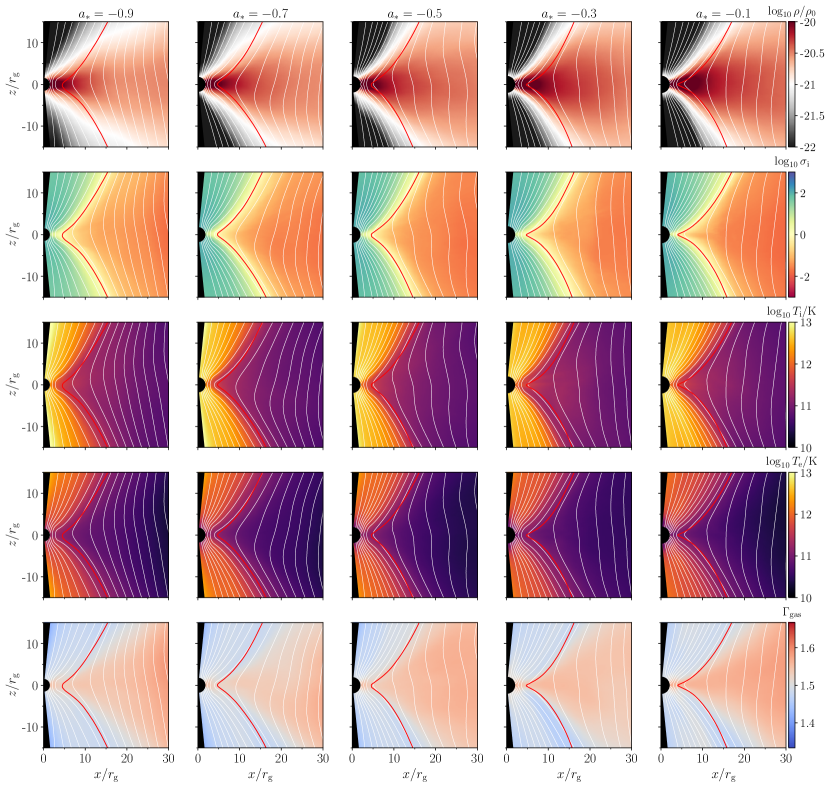
Figure 3: Poloidal profiles of retrograde radiative simulations. We plot the same quantities as in Figure 2 for the retrograde radiative simulations am9_radk, am7_radk, am5_radk, am3_radk, and am1_radk.

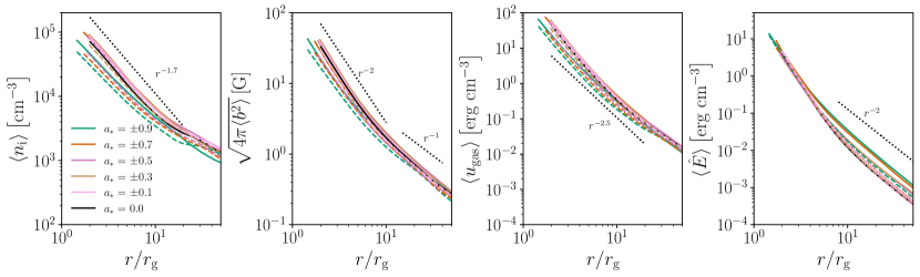
Figure 4: Radial profiles of time-averaged simulation quantities. From left to right, we plot radial profiles of the averaged ion number density $\langle n_{\rm i}\rangle$, the fluid frame magnetic field strength in Gauss, $\sqrt{4\pi\langle b^{2}\rangle}$, the gas internal energy density $\langle u_{\rm gas}\rangle$, and the fluid-frame radiation energy density $\langle\hat{E}\rangle$. All quantities are averaged in time, azimuth, and polar angle using Equation 28. The profiles for prograde simulations are shown in solid lines and profiles for retrograde simulations are shown in dashed lines. Dot-dashed lines indicate characteristic radial falloffs for each quantity.

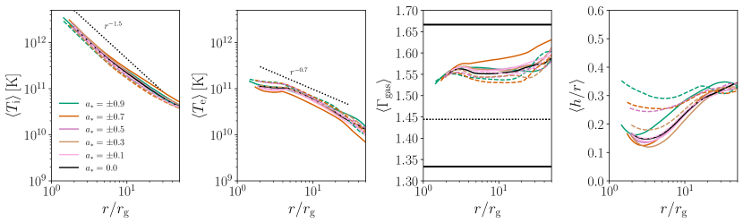
Figure 5: More radial profiles of time-averaged simulation quantities. From left to right, we plot radial profiles of the averaged ion temperature $\langle T_{\rm i}\rangle$, the electron temperature $\langle T_{\rm e}\rangle$, the gas adiabatic index $\langle\Gamma_{\rm gas}\rangle$ and the disc scale height $\langle h/r\rangle$. The first three quantities are averaged in time, azimuth, and polar angle using Equation 28, and the scale height is computed with Equation 29. The profiles for prograde simulations are shown in solid lines and profiles for retrograde simulations are shown in dashed lines. The solid horizontal lines on the third panel indicate the lower and upper limits of $\Gamma_{\rm gas}$; $\Gamma_{\rm gas}=4/3$ and $\Gamma_{\rm gas}=5/3$ for an ultra-relativistic and non-relativistic gas, respectively. The dotted horizontal line indicates $\Gamma_{\rm gas}=13/9$.

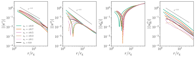
Figure 6: Radial profiles of time-averaged simulation velocities. From left to right, we plot radial profiles of the averaged fluid radial velocity $\langle u^{r}\rangle$, the averaged fluid azimuthal velocity $\langle u^{\phi}\rangle$, the averaged radiation frame radial velocity $\langle u^{r}_{\rm R}\rangle$ and the averaged radiation frame azimuthal velocity $\langle u^{\phi}_{\rm R}\rangle$. All velocity components are in Kerr-Schild coordinates and are averaged in time, azimuth, and polar angle using Equation 28. The profiles for prograde simulations are shown in solid lines and profiles for retrograde simulations are shown in dashed lines.

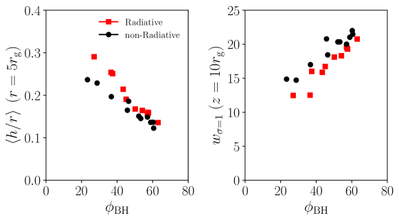
Figure 7: Dependence of disc height and jet width on magnetic flux. The left plot shows values of the disc scale height $\langle h/r\rangle$ computed at radius $r=5\,r_{\rm g}$ with Equation 29 plotted against the corresponding simulation’s averaged value of dimensionless magnetic flux $\phi_{\rm BH}$ (Equation 19). The right plot shows values of the jet width $w$, defined as twice the cylindrical radius of the average $\sigma_{\rm i}=1$ contour (the magenta lines in Figure 2 and Figure 3) at height $z=10\,r_{\rm g}$. In both plots, red squares indicate values computed from the eleven radiative simulations and black circles indicate values taken from the eleven non-radiative simulations.

In Figure 2 and Figure 3, we display poloidal profiles of certain quantities averaged in time (over $t=15000-20000\,t_{\rm g}$) and azimuth (over $2\pi$) for the prograde and retrograde radiative simulations, respectively. In each panel, from top to bottom, we plot the time- and azimuthally-averaged mass density $\rho$, the averaged magnetization parameter $\sigma_{\rm i}$, the ion temperature $T_{\rm i}$, the electron temperature $T_{\rm e}$, and the adiabatic index $\Gamma_{\rm gas}$. In all panels we indicate the averaged $\sigma_{\rm i}=1$ surface in a magenta contour. To indicate average poloidal magnetic field lines, we also plot contours of the average phi-component of the vector potential, computed by integrating the radial magnetic field $B^{r}$ on contours of constant $r$:

$$A_{\phi}=\int_{\theta}B^{r}\sqrt{-g}\mathop{}\!\mathrm{d}\theta,$$ (27)

where in the integral we use the time- and azimuthally-averaged radial field $B^{r}$ in Kerr-Schild coordinates.

The poloidal profiles in Figure 2 and Figure 3 indicate that all the radiative simulations have average structures close to the black hole that are characteristic for hot magnetically arrested discs. Each simulation features thick discs with a large scale height and wide jets, as traced either by the $\sigma_{\rm i}=1$ surface or the last $A_{\phi}$ contour to thread the black hole. The jet region is strongly magnetized, with $\sigma_{\rm i}$ reaching the ceiling value of the simulation. While the discs at large radii are weakly magnetized, the average $\sigma_{\rm i}$ exceeds unity out to $r\approx 5\,r_{\rm g}$ in the equatorial plane in all simulations. Since the 230 GHz emission region probed by the EHT extends to $r\approx 5\,r_{\rm g}$ (Event Horizon Telescope Collaboration et al., 2019b), accurate emission modelling of high-magnetization material is essential for interpreting EHT observations.

The ion and electron temperature plots in the third and fourth in Figure 2 and Figure 3 indicate that in the inner $30\,r_{\rm g}$ of the simulation both electrons and ions are hot, $10^{10}\mathrm{K}<T_{\rm i,e}<10^{13}\mathrm{K}$, with both electron and ion temperatures climbing to their highest values in the nearly evacuated jet region and decreasing with radial distance in the equatorial plane. The average electron temperature is less than the average ion temperature throughout the simulation domain, despite the fact that in the K19 heating prescription (Equation 13) delivers most of the heat to electrons in the most highly magnetized regions ($\delta_{\rm e}>0.5$ when $\beta_{\rm i}\ll 1$). This result suggests that radiation plays a key role in these simulations in keeping the electrons cooler than the ions, even in the highly magnetized jet. The last rows of Figure 2 and Figure 3 indicate that the variation of $T_{\rm i,e}$ over the simulation volume results in a combined gas adiabatic index $\Gamma_{\rm gas}$ that is not constant. In particular, in the hot jet region electrons become ultra-relativistic and ions are near-relativistic, and the adiabatic index $\Gamma_{\rm gas}$ decreases from its value in the disc closer to the relativistic limit of $4/3$.

In Figure 4, Figure 5, and Figure 6 we show radial profiles of certain density-weighted quantities for the prograde (in solid lines) and retrograde (in dashed lines) radiative simulations. For a simulation quantity $q$, we define a density-weighted average $\langle q\rangle(r)$ over the $(\theta,\phi,t)$ coordinates as:

$$\langle q\rangle(r)=\frac{\int_{t}\int_{\phi}\int_{\theta}q\rho\sqrt{-g}\;\mathop{}\!\mathrm{d}\phi\mathop{}\!\mathrm{d}\theta\mathop{}\!\mathrm{d}t}{\int_{t}\int_{\phi}\int_{\theta}\rho\sqrt{-g}\;\mathop{}\!\mathrm{d}\phi\mathop{}\!\mathrm{d}\theta\mathop{}\!\mathrm{d}t}.$$ (28)

In Figure 4 we plot the averaged ion number density $\langle n_{\rm i}\rangle$, the averaged fluid-frame magnetic field strength in Gauss $\sqrt{4\pi\langle b^{2}\rangle}$, the average fluid internal energy density $\langle u_{\rm gas}\rangle$ and the average radiation energy density in the fluid frame $\langle\hat{E}\rangle$. We find that the radiative simulations at all values of black hole spin show similar power-law falloffs for these disc-averaged quantities. The density falls off as ${\approx}r^{-1.7}$, though the retrograde simulations exhibit lower densities and slightly shallower falloffs. At larger radii the magnetic field strength falls off as ${\approx}r^{-1}$, but at small radii $r<10\,r_{\rm g}$ the magnetic field strength falls off more steeply as ${\approx}r^{-2}$; this change in the slope of $b(r)$ indicates that the disc magnetic field becomes poloidally dominated close to the black hole, which is a key signature of magnetically arrested accretion. The gas internal energy density $u_{\rm gas}$ falls off as ${\approx}r^{-2.5}$ in the inner disc, but the retrograde discs tend to have slightly lower values. Finally, the radiation energy density $\hat{E}$ has a falloff consistent with free streaming ${\approx}r^{-2}$ outside of $r=10\,r_{\rm g}$ but falls off more steeply interior to this radius, indicating that most of the bolometric luminosity is produced in the inner region of the accretion flow.

In Figure 5 we plot the density-weighted average ion and electron temperatures $\langle T_{\rm i}\rangle$, $\langle T_{\rm e}\rangle$ in Kelvin, the average gas adiabatic index $\langle\Gamma_{\rm gas}\rangle$, and the disc scale height $\langle h/r\rangle$, defined as

$$\langle h/r\rangle(r)=\frac{\int_{t}\int_{\theta}\int_{\phi}\left|\pi/2-\theta\right|\rho\sqrt{-g}\;\mathop{}\!\mathrm{d}\theta\mathop{}\!\mathrm{d}\phi\mathop{}\!\mathrm{d}t}{\int_{t}\int_{\theta}\int_{\phi}\rho\sqrt{-g}\;\mathop{}\!\mathrm{d}\phi\mathop{}\!\mathrm{d}\theta\mathop{}\!\mathrm{d}t}.$$ (29)

Again, we see that the average value of the electron temperature is less than the averaged ion temperature in the inner disc, though the two species have different temperature profiles, with the ion temperature falling off more steeply compared to the relatively flat electron temperature profile for $r<10\,r_{\rm g}.$ The retrograde simulations tend to have slightly cooler ions and slightly hotter electrons than the corresponding prograde simulations, though this spin dependence is mild.

The third panel of Figure 5 shows the average value of the combined adiabatic index $\Gamma_{\rm gas}$ computed with Equation 2. Throughout the inner disc $r<50\,r_{\rm g}$, the radiative simulations produce values of $\Gamma_{\rm gas}$ between the non-relativistic limit $\Gamma_{\rm gas}=5/3$ and the equal-temperature value for relativistic electrons and non-relativistic ions $\Gamma_{\rm gas}=13/9$; the average $\Gamma_{\rm gas}\approx 1.55$. The retrograde simulations have slightly hotter (and thus more relativistic) electrons; correspondingly, their average adiabatic indices are slightly lower than their prograde counterparts. The $a_{*}=0.7$ simulation stands out with a value of $\Gamma_{\rm gas}$ elevated by ${\approx}20\%$ compared to the other prograde simulations; this seems to be the result of the electrons in this simulation being slightly cooler in comparison to the $a_{*}=0.5$ and $a_{*}=0.9$ simulations, though the reason for this systematic difference is not immediately clear. The disc scale height is strongly spin dependent, with retrograde simulations showing larger values of $\langle h/r\rangle$ in the inner disc where the fluid transitions from counter-rotating to co-rotating with the black hole. The retrograde simulations with more rapidly spinning black holes have the largest values of $\langle h/r\rangle$; this result is consistent with what was observed in Narayan et al. (2022).

In Figure 6 we plot the absolute value of the density-weighted averaged radial and azimuthal 4-velocities $\langle u^{r}\rangle$ and $\langle u^{\phi}\rangle$ in Kerr-Schild coordinates. We also plot the corresponding 4-velocity components for the radiation frame $\langle u^{r}_{\rm R}\rangle$, $\langle u^{\phi}_{\rm R}\rangle$. The fluid’s radial velocity increases toward the black hole with an ${\approx}r^{-1.2}$ dependence; retrograde simulations have a larger inflow velocity than prograde simulations. The angular velocity has a Keplerian fall-off ${\approx}r^{-1.5}$, though with slightly sub-Keplerian values of $u^{\phi}$. The retrograde simulations all show a reversal in the sign of $u^{\phi}$ at a spin-dependent radius; the more rapidly spinning black holes in retrograde simulations force the fluid to co-rotate at larger radii.

The radial component of the radiation-frame four-velocity changes sign in all simulations in the inner $5\,r_{\rm g}$, indicating that the bulk of the radiation in the inner accretion disc falls into the black hole while farther out radiation escapes to infinity (this does not indicate that no radiation from the inner $5\,r_{\rm g}$ escapes, as Figure 6 shows only the density-weighted average of $u_{\rm R}^{r}$). The azimuthal component of the radiation frame velocity is highly spin-dependent, with more rapidly spinning prograde and retrograde black holes producing larger values of $|u_{\rm R}^{\phi}|$ and thus radiation that is more highly beamed than black holes with lower spin.

Comparing Figure 2 and Figure 3, we can see by eye that the jets in the prograde simulations (marked by the $\sigma_{\rm i}=1$ contours) are somewhat wider than in the corresponding retrograde simulations; this is a result of the dependence of the jet width and disc scale height $\langle h/r\rangle$ on the magnetic flux $\phi_{\rm BH}$ noted in Narayan et al. (2022). In Figure 7 we compare the value of the disc scale height $\langle h/r\rangle$ at $r=4\,r_{\rm g}$ as a function of the dimensionless horizon flux $\phi_{\rm BH}$ for the radiative and non-radiative simulations. We also show the jet width for all simulations as a function of $\phi_{\rm BH}$, where we define the jet width $w$ as twice the cylindrical radius of the time- and phi-averaged $\sigma=1$ at height $z=10\,r_{\rm g}$.

In Figure 7 we reproduce the qualitative trend of Narayan et al. (2022) that the disc scale height decreases with the magnetic flux $\phi_{\rm BH}$ and the jet width correspondingly increases. The radiative simulations systematically have larger scale heights and narrower jets than their non-radiative counterparts, with the radiative discs (jets) being ${\approx}$15% thicker (${\approx}10\%$ narrower) than their non-radiative counterparts. This systematic offset is likely a result of the difference in the adiabatic index $\Gamma_{\rm gas}$ between the radiative simulations, where $\Gamma_{\rm gas}$ is solved for self-consistently and takes on a disc-averaged value $\Gamma_{\rm gas}{\approx}1.55$, compared with the non-radiative simulations, where $\Gamma_{\rm gas}$ is fixed at $\Gamma_{\rm gas}=13/9$. The larger effective adiabatic index in the radiative simulation implies that radiative discs with similar internal energy densities to their non-radiative counterparts will have ${\approx}25\%$ more gas pressure; this systematically increased pressure in the radiative simulations likely increases the scale height and decreases the width of the magnetized funnel. Naively, we may have expected that the discs in the radiative simulations would be thinner than the discs in the corresponding non-radiative simulations due to an overall loss of internal energy density from cooling; however, because the radiative efficiency is low $(3-35\%$), the larger difference in the adiabatic indices from self-consistently tracking the electron and ion species in the radiative simulations has a larger effect than radiative cooling in modifying the gas pressure.

4.3 Temperature Ratio

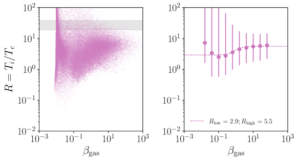
Figure 8: Temperature ratio $R=T_{\rm i}/T_{\rm e}$ versus $\beta_{\rm gas}$ in simulation ap5_radk. In the left panel, we show a scatter plot of $R$ against $\beta_{\rm gas}$ with points sampled randomly from all cells within $r<25\,r_{\rm g}$ over the time range $15000-20000\,t_{\rm g}$ in the simulation. We exclude cells with $\sigma_{\rm i}>25$, as these cells are also excluded in radiative transfer for the 230 GHz images reported in subsection 4.4. The initial range of $R$ when the simulation is re-started from single-fluid GRMHD data at $t=10000\,t_{\rm g}$ is indicated with the gray band. In the right panel, we plot the left panel data binned in 10 equally spaced logarithmic bins; data points indicate the median value in each bin and error bars indicate the 68% credible interval. We fit the binned data to the Mościbrodzka et al. (2016) prescription Equation 30; the resulting fit for parameters $R_{\rm low}=2.5$, $R_{\rm high}=5.6$ is indicated by the dashed curve.

Next we investigate the electron-to-ion temperature ratio $R=T_{\rm i}/T_{\rm e}$ in individual snapshots of our radiative, two-temperature simulations. To simulate horizon-scale synchrotron images from single-fluid GRMHD simulations without self-consistent temperature evolution, the standard approach (e.g. Event Horizon Telescope Collaboration et al., 2019b, 2022b, 2021b) is to use the Mościbrodzka et al. (2016) phenomenological function $R(\beta_{\rm gas})$:

$$R=R_{\rm low}\frac{1}{1+\beta^{2}_{\rm gas}}+R_{\rm high}\frac{\beta^{2}_{\rm gas}}{1+\beta^{2}_{\rm gas}}.$$ (30)

In the Mościbrodzka et al. (2016) “$R-\beta$” model (Equation 30), the ion-to-electron temperature ratio is a fixed function of the gas plasma beta parameter and transitions from a value $R=R_{\rm low}$ in highly magnetized regions $\beta_{\rm gas}\ll 1$ to $R=R_{\rm high}$ in weakly magnetized regions $\beta_{\rm gas}\gg 1$. Because electron heating functions from plasma turbulence simulations (Howes, 2010; Kawazura et al., 2019) preferentially heat electrons at low $\beta_{\rm gas}$ and preferentially heat ions at high $\beta_{\rm gas}$, libraries of simulated 230 GHz images used for interpreting EHT results tend to adopt $R_{\rm low}=1$ and sample several values $R_{\rm high}>1$ Event Horizon Telescope Collaboration et al. (2019b), though in simulations of M87* Event Horizon Telescope Collaboration et al. (2021b, 2023) also explored models with $R_{\rm low}=10$ to simulate the effect of radiative cooling of electrons in high magnetization regions.

With our radiative, two-temperature simulation suite with electrons and ions heated by the Kawazura et al. (2019) plasma turbulence prescription, we can investigate the dependence of $R$ against $\beta_{\rm gas}$ and compare it to the standard Mościbrodzka et al. (2016) prescription for single-fluid GRMHD, Equation 30 (see also Dihingia et al., 2023). In the left panel of Figure 8, we show a scatter plot of the electron-to-ion temperature ratio versus the plasma beta parameter $\beta_{\rm gas}$ from randomly chosen cells in the inner $25\,r_{\rm g}$ of the simulation ap5_radk in the time range $15000-20000\,t_{\rm g}$. The gray shaded region in the left panel of Figure 8 indicates the range of initial temperature ratios $R_{\rm init}=19-38$ set when we initialize the two-temperature plasma. The range of $\beta_{\rm gas}$ in the simulation is limited by an overall floor $b^{2}/u_{\rm gas}<200$ used in KORAL along with the ceiling $\sigma_{\rm max}=100$ to ensure numerical stability in highly magnetized regions.

In the left panel of Figure 8 we can see that in our two-temperature simulations, the temperature ratio $R$ typically takes on intermediate values $R\approx 1-10$, except for in the most magnetized regions close to the $\beta_{\rm gas}$ floor where radiative cooling is strongest. Furthermore, we see that $R$ is not a single-valued function of $\beta_{\rm gas}$; there can be up to an order of magnitude of scatter in $R$ for simulation cells with a given $\beta_{\rm gas}$. The scatter in the $R-\beta_{\rm gas}$ relationship arises because the electron and ion temperatures of a packet of gas depend not only on the local heating fraction $\delta_{\rm e}$ through Equation 13, but also on the thermal history of the gas packet through transport, adiabatic compression/expansion, and radiation.

In the right panel of Figure 8 we bin the $R$ values in 10 equally spaced logarithmic bins ranging from $\beta_{\rm gas}=10^{-2}$ to in $\beta_{\rm gas}=10^{2}$ and plot the resulting median values and $68\%$ credible interval for each bin. We fit the two-parameter Mościbrodzka et al. (2016) model, Equation 30, to the binned data, resulting in a model with $R_{\rm low}=2.5$, $R_{\rm high}=5.6$. While we only show results for model ap5_radk here, the distributions of $R$ and the fitted values of $R_{\rm low}$, $R_{\rm high}$ for the simulations with different black hole spin values are similar; we summarize the fitted $R_{\rm low}$, $R_{\rm high}$ values for all the radiative simulations in Table 3.

Model	$R_{\rm low}$	$R_{\rm high}$
ap9_radk	3.2	5.4
ap7_radk	3.5	8.1
ap5_radk	2.5	5.6
ap3_radk	2.8	5.6
ap1_radk	2.2	5.5
a0_radk	1.8	5.7
am1_radk	2.1	4.8
am3_radk	1.6	5.0
am5_radk	2.2	4.6
am7_radk	1.6	4.2
am9_radk	2.2	4.6

Table 3: Mościbrodzka et al. (2016) electron temperature parameters $R_{\rm low}$,$R_{\rm high}$ fit to binned radiative simulation data for all eleven radiative simulations. For each simulation we bin raw $R,\beta_{\rm i}$ values from simulation snapshots and fit Equation 30 as described in Figure 8.

Our radiative, two-temperature simulations heated by sub-grid plasma turbulence prefer moderate ion-to-electron temperature ratios, summarized by moderate values of the fitted Mościbrodzka et al. (2016) parameters $R_{\rm low}\approx 2$, $R_{\rm high}\approx 5$. In our simulations, close to the black hole electrons are only moderately cooler than ions, even with strong radiative cooling. This moderate temperature ratio is consistent with results for 2D radiative two-temperature simulations at similar accretion rates heated by the Howes (2010) electron heating prescription in Dihingia et al. (2023). Notably, most single fluid MAD GRMHD models that satisfy EHT polarimetric constraints of M87* have higher values $R_{\rm high}\gtrsim 80$, resulting in an overall much cooler population of electrons (Event Horizon Telescope Collaboration et al., 2021b).

4.4 Images

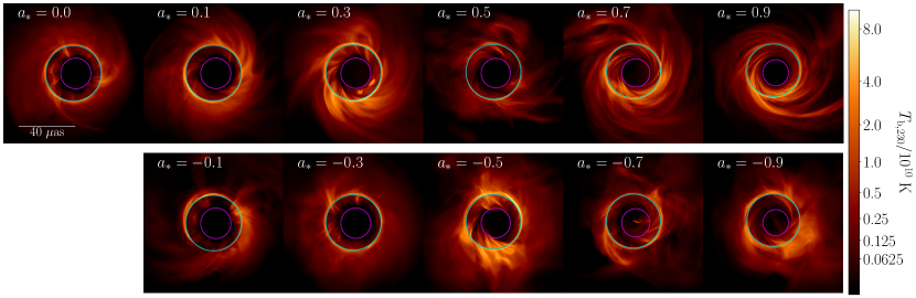
Figure 9: Snapshot images from the eleven radiative simulations. Synchrotron images were produced at 230 GHz using ipole; prograde simulations (top row) have an observer inclination $\theta_{\rm o}=163\deg$ and retrograde simulations (bottom row) have an observer inclination $\theta_{\rm o}=17\deg$, such that in all simulations the black hole spin is oriented $163\deg$ from the line of sight; the spin vector points to the East (left) of the image (Mertens et al., 2016). Images are plotted in units of brightness temperature $T_{\rm b}$ in a gamma colour scale with image intensities $I$ scaled as $I^{1/4}$. The cyan curve in each image is the “critical curve” that indicates the position of the multiply-lensed photon ring (Johnson et al., 2020); the magenta curve denotes the direct image of the event horizon, or “inner shadow” edge (Chael et al., 2021).

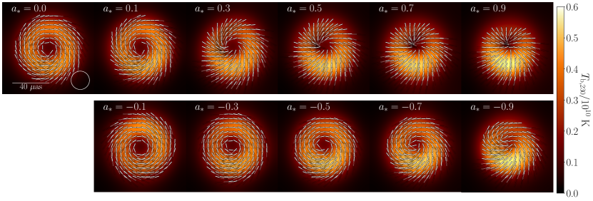
Figure 10: Averaged images from the eleven radiative simulations blurred to EHT resolution. Images from each simulation were blurred to the EHT $20\,\mu$as resolution with a circular Gaussian kernel (indicated with the white circle in the upper left image) and time averaged over the range $15000-20000\,t_{\rm g}.$ Images are displayed in a linear scale, and ticks indicate the EVPA direction across the image.

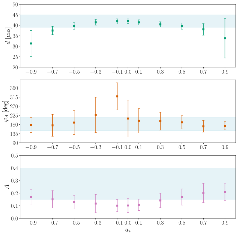
Figure 11: Total intensity image statistics. From top to bottom we plot the ring diameter $d$ (Equation 31), image position angle $\varphi_{A}$ (Equation 33) and image asymmetry parameter $A$ (Equation 32) for each radiative simulation as a function of spin $a_{*}$. We plot the mean value and $1\sigma$ error bars from snapshots in the range $15000-20000\,t_{\rm g}$. The blue shaded ranges indicate the range of values measured from EHT observations of M87* in 2017 Event Horizon Telescope Collaboration et al. (2019a) and 2018 Event Horizon Telescope Collaboration et al. (2024a).

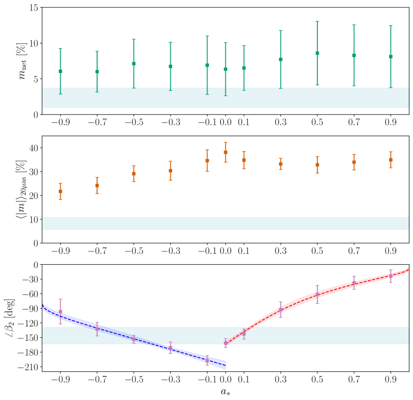
Figure 12: Polarimetric image statistics. From top to bottom we plot the net linear polarization fraction $m_{\rm net}$ (Equation 34), the EHT-scale average linear polarization fraction $\langle|m|\rangle$ (Equation 35) and the phase of the linear polarization’s second Fourier coefficient $\angle\beta_{2}$ (Equation 36, Palumbo et al. 2020). We plot the mean value and $1\sigma$ error bars from snapshots in the range $15000-20000\,t_{\rm g}$. The blue shaded ranges indicate the range of values measured from EHT observations of M87* in 2017 Event Horizon Telescope Collaboration et al. (2021a). The dashed blue and red lines indicate fits to the prograde and retrograde simulation results for $\angle\beta_{2}$ as a function of $a_{*}$ using the functional form Equation 37. The shaded blue and red regions represent the $99\%$ credible interval on the fitting functions for the prograde and retrograde simulations derived from sampling the fit covariance.

In Figure 9 we show $230$ GHz image snapshots selected from all eleven radiative simulations computed with ipole (Mościbrodzka & Gammie, 2018). The observer inclination in our simulated images is set to $\theta_{\rm o}=163\deg$ for the prograde discs and $\theta_{\rm o}=17\deg$ for the retrograde discs; the images are plotted in a gamma colour scale with intensity $I$ scaled as $I^{1/4}$. The snapshot images in Figure 9 show similar intensity distributions to images from single-fluid GRMHD MAD simulations known to fit total intensity observations of M87* (Event Horizon Telescope Collaboration et al., 2019b). Notably, the optically thin photon ring feature from light rays lensed $>180\deg$ (Johnson et al., 2020) is apparent in each simulation (indicated by the cyan contour); the “inner shadow” feature, or the direct image of material just outside the event horizon (Chael et al. 2021, indicated by the magenta contour), is also visible.

In Figure 10 we show the $230$ GHz images time-averaged over the interval $15000-20000\,t_{\rm g}$ and blurred to the EHT resolution of 20 $\mu$as with a circular Gaussian kernel. The time-averaged images are displayed in a linear colour scale; we also display the averaged pattern of linear polarization with tick marks indicating the direction of the electron vector position angle (EVPA) across the image. It is apparent in the averaged EHT resolution images that the direction and magnitude of the asymmetry in the image is spin-dependent, with images from more rapidly spinning black holes exhibiting more pronounced brightness asymmetry (Event Horizon Telescope Collaboration et al., 2019b, 2022b; Medeiros et al., 2022). It is also apparent that the pattern of linear polarization is highly spin-dependent, with lower-spin images displaying more azimuthal polarization patterns and more rapidly spinning black holes displaying more radial polarization patterns (Palumbo et al., 2020; Event Horizon Telescope Collaboration et al., 2021b).

For each blurred image snapshot, we follow Event Horizon Telescope Collaboration et al. (2019a) and compute several summary statistics for both total intensity and linear polarization. We work in polar coordinates $(\rho,\varphi)$ in the image plane. We compute the ring diameter $d$ by finding the radius $\rho_{\rm pk}$ of peak intensity in radial profiles $I(\rho)$ at fixed image position angles and averaging over $\varphi$:

$$d =2\left\langle\rho_{\rm pk}(\varphi)\right\rangle_{\varphi\in\left[0,2\pi\right]}.$$ (31)

Similarly, the ring width $w$ is the mean full width at half maximum (FWHM) value of the individual profiles. With $d$ and $w$ defined, the inner ring radius is $\rho_{\rm in}=(d-w)/2$ and the outer ring radius is $\rho_{\rm out}=(d+w)/2$. We define the ring asymmetry factor $A$ and position angle $\varphi_{A}$ as

$$A =\left\langle\frac{\left|\int_{\varphi}I(\rho,\varphi)e^{i\varphi}\mathop{}\!\mathrm{d}\varphi\right|}{\int_{\varphi}I(\rho,\varphi)\mathop{}\!\mathrm{d}\varphi}\right\rangle_{\rho\in\left[\rho_{\rm in},\rho_{\rm out}\right]},$$ (32)

$$\varphi_{A} =\left\langle\arg\left[\int_{\varphi}I(\rho,\varphi)e^{i\varphi}\mathop{}\!\mathrm{d}\varphi\right]\right\rangle_{\rho\in\left[\rho_{\rm in},\rho_{\rm out}\right]}.$$ (33)

The image position angle $\varphi$ is measured in degrees East of North (counter-clockwise from the top of the image in Figure 10).

In Figure 11 we plot the mean values of $d,A$, and $\varphi_{A}$ for each simulation, along with their $1\sigma$ error bars computed from snapshots over the time range $15000-20000\,t_{\rm g}$. For the position angle $\varphi_{A}$ we use the circular mean and standard deviation. We compare our simulation results for these quantities to conservative ranges derived from EHT observations of M87* reported in Event Horizon Telescope Collaboration et al. (2019a, 2024a), which we indicate in the blue bands in Figure 11. In particular, we take the EHT ranges as $d\in\left[39,45\right]\mu$as, $A\in\left[0.15,0.4\right]$, and $\varphi_{A}\in\left[150,215\right]\deg$.

Nearly all the radiative, two-temperature simulations naturally satisfy the observed ranges of total intensity summary statistics derived from EHT observations in Event Horizon Telescope Collaboration et al. (2019a, 2024a). At our fixed value of black hole mass $M=6.5\times 10^{9}M_{\odot}$ and distance $D=16.8$ Mpc, the ring diameter in the simulated images decreases with black hole spin as the projected size of the black hole event horizon shrinks. The $a_{*}=\pm 0.9$ simulations have median image ring diameters smaller than the observed range for M87*, but we do not account for uncertainty in the measurement of the black hole mass or distance here. The image position angle $\varphi_{A}$ shows a mild dependence on spin, with more rapidly spinning simulations having slightly smaller values of $\varphi_{A}$. As seen in Figure 10, the magnitude of the image asymmetry $A$ is larger for more rapidly spinning black holes, though all our simulations satisfy the observed ranges within $1\sigma$.

Notably, the $a_{*}=-0.1$ simulation am1_radk has a position angle offset by $90-180\deg$ from the rest of the retrograde simulations. This indicates that the $a_{*}=-0.1$ simulation has its asymmetry direction set by by Doppler beaming from the sense of rotation of the retrograde accretion disc, not the spin direction of the black hole; flipping the viewing orientation of the $a_{*}=-0.1$ simulation from $\theta_{\rm o}=17\deg$ to $\theta_{\rm o}=163\deg$ (so the spin vector points West) shifts the position angle in line with observations. This result indicates that the Event Horizon Telescope Collaboration et al. (2019b) inference that the asymmetry direction of the near-horizon synchrotron ring image is set by the rotation sense of the black hole and not that of the accreting material only holds for moderately to rapidly spinning black holes with $|a_{*}|\gtrsim 0.3$. The frame-dragging effect in the weakly spinning $a_{*}=-0.1$ simulation is not powerful enough to reverse the rotation direction of the retrograde flow in the 230 GHz emitting region, so the asymmetry direction in the image in this case is set by the large-scale flow, as it is in the $a_{*}=0$ simulation.

We next turn to image-averaged linear polarimetric quantities defined in (Event Horizon Telescope Collaboration et al., 2021a, b). Working with images blurred to $20\,\mu$as, the net polarization fraction $m_{\rm net}$ and the average linear polarization at the EHT resolution are:

$$m_{\rm net} =\frac{\left|\int_{y}\int_{x}\mathcal{P}(x,y)\mathop{}\!\mathrm{d}x\mathop{}\!\mathrm{d}y\right|}{\int_{y}\int_{x}I(x,y)\mathop{}\!\mathrm{d}x\mathop{}\!\mathrm{d}y},$$ (34)

$$\langle|m|\rangle =\frac{\int_{y}\int_{x}\left|\mathcal{P}(x,y)\right|\mathop{}\!\mathrm{d}x\mathop{}\!\mathrm{d}y}{\int_{y}\int_{x}I(x,y)\mathop{}\!\mathrm{d}x\mathop{}\!\mathrm{d}y},$$ (35)

Where $x,y$ are image coordinates, $I$ is the image total intensity, and $\mathcal{P}=Q+iU$ is the complex linear polarization derived from the $Q$ and $U$ Stokes parameters. The $\beta_{2}$ parameter (Palumbo et al., 2020) is defined as the complex amplitude of the second Fourier mode around the (blurred) ring:

$$\beta_{2}=\frac{\int_{\varphi}\int_{\rho}\mathcal{P}(\rho,\varphi)e^{-2i\varphi}\rho\mathop{}\!\mathrm{d}\rho\mathop{}\!\mathrm{d}\varphi}{\int_{\varphi}\int_{\rho}I(\rho,\varphi)\rho\mathop{}\!\mathrm{d}\rho\mathop{}\!\mathrm{d}\varphi}.$$ (36)

For each radiative simulation, we plot the median values of $m_{\rm net},\langle|m|\rangle$, and the phase $\angle\beta_{2}$, in Figure 12 along with $1\sigma$ error bars from all snapshots in the time interval $15000-20000\,t_{\rm g}$. For $\angle\beta_{2}$, we use the circular mean and standard deviation. We compare the results from each simulation with the observed ranges from EHT polarimetric observations of M87* reported in (Event Horizon Telescope Collaboration et al., 2021a); $m_{\rm net}\in\left[1.0,3.7\right]\%$, $\langle|m|\rangle\in\left[5.7,10.7\right]\%$, $\angle\beta_{2}\in\left[-163,-129\right]\deg$, indicated by the shaded blue rectangles in Figure 12.

While our radiative simulations all naturally reproduce the total intensity summary statistics from M87* EHT images, they do not satisfy the observed polarimetric constraints. Most notably, the radiative simulations are too polarized, with linear polarization fractions $\langle|m|\rangle$ measured at EHT scales that are a factor of ${\approx}2-10$ times too large compared with observations. This over-polarization is likely a result of the electrons in our simulations being too hot, as indicated by the moderate values of $R=T_{\rm i}/T_{\rm e}$ measured in subsection 4.3. In Event Horizon Telescope Collaboration et al. (2021b), 230 GHz single-fluid GRMHD images are mostly depolarized by differential internal Faraday rotation along different photon trajectories across the image; strong Faraday rotation in a turbulent plasma rotates the EVPAs in adjacent pixels by different amounts, causing an overall depolarization when the image is blurred to 20 $\mu$as resolution (Ricarte et al., 2020). Faraday rotation is more effective in cold plasmas, with rotation suppressed as $1/T^{2}_{\rm e}$ (Jones & Hardee, 1979). The median values of $\langle|m|\rangle$ for the two-temperature MAD models reported here are roughly consistent with the $R_{\rm low}=1$, $R_{\rm high}=10$ MAD M87* model set reported in Event Horizon Telescope Collaboration et al. (2021b), Figure 26. While the EHT has not yet claimed a measurement of $R$ in the emitting region from M87* observations, passing MAD models for M87* in the EHT simulation library prefer large values of the ion-to-electron temperature ratio $R_{\rm high}\approx 80-160$ in order to produce sufficient image depolarization (Event Horizon Telescope Collaboration et al., 2021b). If it is indeed a consequence of Faraday depolarization, the observed large degree of image polarization in M87* (Event Horizon Telescope Collaboration et al., 2021a) likely requires much cooler electrons than are produced in two-temperature simulations with electrons heated with the K19 turbulent heating prescription.

The quantity $\angle\beta_{2}$ quantifies the pattern of the linear polarization spiral in near-horizon images, with $\beta_{2}=0$ corresponding to radial polarization and $\beta_{2}=\pm 180$ corresponding to azimuthal polarization vectors. The value of $\angle\beta_{2}$ probes the pitch angle of the underlying magnetic field in the 230 GHz emission region, which is strongly influenced by the black hole spin. More rapidly spinning black holes more efficiently wind up their magnetic fields in powering Blandford & Znajek (1977) electromagnetic outflows, producing more toroidal fields in the EHT emission region and thus more radial EVPA patterns. In addition, the sign of $\angle\beta_{2}$ encodes the relative direction of the toroidal and poloidal magnetic fields. For a black hole spin vector oriented $163\deg$ to the line of sight (Mertens et al., 2016; Event Horizon Telescope Collaboration et al., 2019b), negative values of $\angle\beta_{2}$ (corresponding to right-handed EVPA spiral) indicate magnetic field lines swept back by the black hole spin and thus capable of powering an energy-extracting BZ outflow (Chael et al., 2023).

The values of $\angle\beta_{2}$ in our radiative simulations plotted in Figure 12 reproduce the observed qualitative trend with spin first reported in Palumbo et al. (2020). Notably, the polarization spiral in the $a_{*}=-0.1$ simulation am1_radk has the opposite sense to the rest of the simulations, with $\angle\beta_{2}{\approx}160\deg$ when the observer inclination $\theta_{\rm o}=163\deg$. This discrepancy indicates that the magnetic field pitch angle in the EHT emission region is set by the large-scale retrograde accretion flow instead of the black hole spin direction for the weakly spinning $a_{*}=-0.1$ black hole, just like the asymmetry position angle in Figure 11.

In the BZ monopole model, the ratio of the Kerr-Schild poloidal to radial magnetic field strength is proportional to $\Omega_{\rm H}$, the angular frequency of the event horizon (Blandford & Znajek, 1977; McKinney & Gammie, 2004). We find that we can fit a simple two-parameter functional form for $\angle\beta_{2}(\Omega_{\rm H})$ to the measured $\angle\beta_{2}$ from the 230 GHz images from the radiative simulations:

$$\left[\angle\beta_{2}\right]_{\rm fit}=2\arctan\left[\frac{-C_{0}}{\left|\Omega_{\rm H}\right|}\right]+C_{1}.$$ (37)

In Equation 37, the parameter $C_{0}$ encodes how rapidly fieldlines are wound up with increasing black hole spin, while $C_{1}$ provides an overall constant shift in the zero-spin value of $\angle\beta_{2}$. We find that this model fits the simulation results well when applied separately to the prograde and retrograde simulations. For the retrograde simulation fit, we find $C_{0}=0.26,C_{1}=-26\deg$ and for the prograde simulations we find $C_{0}=0.11,C_{1}=17\deg$. The discrepancy in values of $\angle\beta_{2}$ and the fitting function results for the prograde and retrograde simulations indicates that the initial condition of the retrograde accretion disc reduces both the rate at which the pitch angle of the field structure increases with spin and the zero value of $\angle\beta_{2}$. As a result, a retrograde simulation at a given absolute value of black hole spin will have an overall more toroidal EVPA pattern than its prograde counterpart.

We note again that the average polarization/magnetic field pitch angle encoded in $\angle\beta_{2}$ is strongly dependent on black hole spin. If we ignore the fact that none of our simulations satisfy EHT constraints on $\langle|m|\rangle$, comparing EHT measurements of $\angle\beta_{2}$ to our simulations selects a retrograde or very modestly prograde black hole spin, $a_{*}\in\left[-0.7,0.2\right]$ for M87*. This inference and the trend for $\angle\beta_{2}$ presented for the radiative simulations in Figure 12 is consistent with results from our non-radiative simulations, with only small shifts in $\angle\beta_{2}$ on the order of ${\approx}10\deg$ from Faraday rotation when changing $R_{\rm low}$, $R_{\rm high}$ (see also Chael 2024, Figure 3 for $\angle\beta_{2}$ values from the MAD simulations of Narayan et al. (2022)). As in Event Horizon Telescope Collaboration et al. (2021b), we find that raytracing the single-fluid GRMHD simulations with larger values of $R_{\rm high}=80-160$ is necessary to reduce $\langle|m|\rangle$ to within the measured EHT range.

5 Discussion and Conclusions

In this paper we present the first systematic survey of two-temperature, radiative GRMHD simulations of M87* with mass accretion rates scaled to produce the flux density observed by the EHT at 230 GHz (Event Horizon Telescope Collaboration et al., 2019a). We ran eleven 2TGRRMHD simulations in the code KORAL with electrons heated by the Kawazura et al. (2019) sub-grid prescription derived from gyrokinetic simulations of plasma turbulence. We find that our simulations have accretion rates $\dot{M}=(0.5-1.5)\times 10^{-6}\dot{M}_{\rm Edd}$ and radiative efficiencies $\epsilon_{\rm rad}=3-35\%$, consistent with results from non-radiative simulation fits to EHT observations in (Event Horizon Telescope Collaboration et al., 2021b). We observe that the trends of bulk properties of our simulations with spin are not affected by the addition of radiation at these low radiative efficiencies; in particular, the radiative and non-radiative simulations produce near-identical results for the average horizon magnetic flux $\phi_{\rm BH}$, outflow efficiency $\eta$, and spindown parameter $s$.

The ion and electron temperature profiles of our simulations are relatively independent of the black hole spin, with the electron temperature being ${\approx}5$ times cooler than the ion temperature in the accretion disc. The disc electrons in our simulations are moderately relativistic, and the combined electron-ion fluid has an effective adiabatic index $13/9<\Gamma_{\rm gas}<5/3$, while the adiabatic index in the hot jet region is lower, $4/3<\Gamma_{\rm gas}<13/9$. We find that the larger value of the adiabatic index in the accretion disc affects global structures in the simulation when compared to our fiducial single-fluid GRMHD simulations with fixed $\Gamma_{\rm gas}=13/9$; in particular, the disc scale height in our radiative simulations is larger than in their non-radiative counterparts, and the jet width is correspondingly smaller.

Our simulations produce values of the temperature ratio $R=T_{\rm i}/T_{\rm e}$ that are not tightly correlated with $\beta_{\rm gas}$; by contrast, the standard approach from post-processing modelling of $R$ in single-fluid GRMHD simulations uses a one-to-one function $R(\beta)$. When fitting the Mościbrodzka et al. (2016) model $R(\beta)$ to our simulation results, we find an effective $R_{\rm low}\approx 2$ and $R_{\rm high}\approx 5$. Our results for the electron temperature are consistent with results from 2D MAD simulations run with the Howes (2010) heating prescription run at comparable accretion rates in Dihingia et al. (2020, 2023).

230 GHz images from our simulations reproduce the total-intensity properties of M87* on event horizon scales observed by the EHT in 2017 (Event Horizon Telescope Collaboration et al., 2019a) and 2018 (Event Horizon Telescope Collaboration et al., 2024a). Our 2TGRRMHD simulations also reproduce the same observed trend of the polarization’s second Fourier mode phase $\angle\beta_{2}$ with spin that is observed in single-fluid MAD simulations (Palumbo et al., 2020) and which directly probes the dragging of magnetic field lines by black hole spin (Chael, 2024). However, our simulations produce linear polarization fractions at the resolution of the EHT beam that are several times too large when compared to observations (Event Horizon Telescope Collaboration et al., 2021a). These large polarization fractions are also seen in single-fluid MAD GRMHD simulations of M87* raytraced with the Mościbrodzka et al. (2016) prescription and small values of the high-$\beta$ ion-to-electron temperature ratio, $R_{\rm high}\mathrel{\raise 1.29167pt\hbox{$<$\kern-7.5pt\lower 4.30554pt\hbox{$\sim$}}}10$ (Event Horizon Telescope Collaboration et al., 2021b). In strongly-magnetized MAD GRMHD simulations, cooler electron temperatures (large effective values of $R_{\rm high}\approx 80-160$) are necessary to produce sufficient internal Faraday rotation to de-polarize the emission to the observed $\langle|m|\rangle\mathrel{\raise 1.29167pt\hbox{$<$\kern-7.5pt\lower 4.30554pt\hbox{$\sim$}}}10\%$ on $20\,\mu$as scales (Event Horizon Telescope Collaboration et al., 2021b, 2023).

The high electron temperatures and correspondingly high polarization fractions in our 2TGRRMHD simulation suite poses a challenge to the interpretation of EHT polarization results. Is it possible to obtain higher ion-to-electron temperature ratio that match values preferred by post-processing modelling of EHT data with physically based models of plasma heating? First, it should be noted that 2TGRRMHD simulations are known to not perfectly identify grid-scale dissipation; their algorithm for calculating the grid-scale viscous heating rate $q^{\rm v}$ produces artificial heating or even negative heating in certain regions (Ressler et al., 2017; Sądowski et al., 2017). The KORAL code attempts to counter any trend toward excess heating by correcting $q^{\rm v}$ to account for additional entropy generated by mixing finite-sized fluid parcels (Sądowski et al. 2017, section 3.1), and recent tests by Mościbrodzka (2024) have not found any dependence of the global species temperatures or simulated images on resolution, as might be expected if finite numerical resolution was introducing excess heating. However, to ensure the numerical method is not responsible for the low $R$ and high polarization values observed here, it would be useful to reproduce the results of our simulation suite with a different numerical implementation. Ideally, alternate algorithms for identifying $q^{\rm v}$ in simulations should be developed to further test these results.

Another source of uncertainty in comparing GRMHD simulations to images of M87* is the treatment of emission from the magnetized jet region. In this work, we adopt a “sigma cut-off” of $\sigma_{\rm cut}=25$, zeroing out 230 GHz emission from all regions with a higher magnetization. A more common practice in the community is to set $\sigma_{\rm cut}=1$, treating emission from all regions where the magnetic field dominates the energy budget as suspect. We find in our simulations between $30-50\%$ of the median 230 GHz flux density comes from the highly magnetized region between $1<\sigma_{\rm i}<25$; we choose to include emission from this region because $\sigma_{\rm i}\approx 1$ gas represents a significant volume of the near-horizon accretion inflow and outflow and contributes meaningfully to the observed emission in MAD systems, while being sufficiently far from the simulation’s ceiling value $\sigma_{\rm max}=100$ to avoid obvious artefacts from density floors (Chael et al., 2019; Chael, 2024). However, adopting a lower value of $\sigma_{\rm cut}$ would result in requiring correspondingly higher values of the accretion rate $\dot{M}$ to reproduce the observed 230 GHz flux density $F_{230}$, resulting in somewhat more efficient electron cooling and more Faraday depth, though a $30-50\%$ increase in accretion rate is likely not sufficient to bring our results for $\langle|m|\rangle$ in line with 230 GHz observations. In the next paper in this series, we will run a detailed comparison of a single two-temperature simulation with accretion rates chosen to reproduce the observed 230 GHz flux density under different $\sigma_{\rm cut}$ assumptions.

While the K19 heating prescription seems to produce electrons that are too hot in MAD simulations to satisfy observational constraints, it may be that another sub-grid heating model exists that supplies a lower $\delta_{\rm e}$ in the 230 GHz emitting region and thus results in cooler electrons and lower polarization from Faraday depolarization. The logical next step is to compare the simulations presented here with an analogous set of simulations heated by magnetic reconnection using the Rowan et al. (2019) (R19) prescription. The R19 prescription provides more heat to electrons at high $\beta$, but in the highly magnetized regions of MAD discs where most 230 GHz emission is produced, R19 may provide lower values of $\delta_{\rm e}$ than the K19 model used in this paper (Chael et al., 2019). Previous studies have found that R19 is preferred to a turbulent heating model in reproducing certain features of M87*’s total intensity jet emission (Chael et al., 2019) and Sgr A*’s total fractional polarization and variability (Chael et al., 2018; Dexter et al., 2020), though Sgr A* is significantly more polarized than M87* on EHT scales (Event Horizon Telescope Collaboration et al., 2021a). However, two recent two-temperature radiative simulation studies targeted at Sgr A* (Salas et al., 2024) and at X-ray binary accretion over a range of accretion rates (Liska et al., 2024) using the Rowan et al. (2017) heating prescription both found modest values of $R\approx 5-10$, suggesting that a simple change of heating model may not produce sufficiently cold electrons to depolarize M87*’s 230 GHz images. In the next paper in this series we will investigate if the R19 reconnection model is more successful in reproducing the observed low horizon-scale polarization fraction in M87*.

In addition to the original K19 heating prescription from Alfvénic turbulence, recent work by Kawazura et al. (2020) has examined the role of compressive driving of a turbulent cascade in altering the resulting electron heating fraction at small scales. Satapathy et al. (2023, 2024) have explored the implications of the Kawazura et al. (2020) model in semi-analytic models and shearing-box simulations, and have found that a larger degree of compressive driving lowers the effective $\delta_{\rm e}$ from the Kawazura et al. (2019) K19 result, with a predicted range of effective temperature ratios $R\approx 5-40$ for $\beta_{\rm gas}\approx 1-10$. Global 2TGRRMHD simulations including an effective subgrid model for turbulent heating modified by compressive modes following Satapathy et al. (2024) are necessary to establish if this change is sufficient to produce polarization fractions for M87* within the measured range for electrons heated by plasma turbulence.

If no plasma heating prescription $\delta_{\rm e}$ can be found that produces sufficiently cold electrons and sufficiently large depolarization in MAD M87* models, it may imply that other changes to the accretion flow structure independent of the electron temperature modelling should be considered. Turbulent field “SANE” models are naturally more depolarized than MAD models at all values of the Mościbrodzka et al. (2016) parameters $R_{\rm high}$, $R_{\rm low}$ due to their more turbulent magnetic fields (Event Horizon Telescope Collaboration et al., 2021b). SANE simulations generally do not satisfy EHT constraints on $\angle\beta_{2}$ and can in some cases be too depolarized to satisfy the observed lower bound on $\langle|m|\rangle$, and EHT simulation scoring largely rules them out as models of M87* when compared to MAD simulations (Event Horizon Telescope Collaboration et al., 2021b). However, if electrons in two-temperature simulations cannot be made sufficiently cool it may be that simulations with a more intermediate level of $\phi_{\rm BH}$ higher than the typical value $\phi_{\rm BH}\mathrel{\raise 1.29167pt\hbox{$<$\kern-7.5pt\lower 4.30554pt\hbox{$\sim$}}}5$ but below the MAD saturation of $\phi_{\rm BH}\approx 50$ may produce more depolarized emission while satisfying EHT constraints on $\beta_{2}$. More broadly, future investigations should explore the effect on the polarization of physics and initial conditions not explored in the standard assumptions of aligned, two-temperature accretion such as disc tilt (White et al., 2019; Chatterjee et al., 2020), large-scale plasma feeding (Guo et al., 2024), anisotropic electron distributions (Galishnikova et al., 2023), and non-zero helium fractions (Wong & Gammie, 2022).

Previous comparisons of 2TGRRMHD simulations to total intensity and pre-EHT observations of Sgr A* (e.g Chael et al., 2018) and M87* (e.g Chael et al., 2019) found only weak preferences for different electron heating mechanisms based on the observational data; prior to the first EHT polarized images, constraining the microscopic plasma heating processes in Sgr A* and M87* with observations did not seem feasible. The advent of robust polarized images from the EHT have changed this paradigm. The results of this first large survey of 2TGRRMHD simulations of M87* indicate that polarized horizon-scale images can strongly constrain models of collisionless plasma heating in hot accretion flows just outside supermassive black holes.

Data Availability

The data from the simulations reported here are available on request. The KORAL code is available at https://github.com/achael/koral_lite.

References

- Blandford & Payne (1982) Blandford R. D., Payne D. G., 1982, MNRAS, 199, 883
- Blandford & Znajek (1977) Blandford R. D., Znajek R. L., 1977, MNRAS, 179, 433
- Chael (2024) Chael A., 2024, MNRAS, 532, 3198
- Chael et al. (2018) Chael A., Rowan M., Narayan R., Johnson M., Sironi L., 2018, MNRAS, 478, 5209
- Chael et al. (2019) Chael A., Narayan R., Johnson M. D., 2019, MNRAS, 486, 2873
- Chael et al. (2021) Chael A., Johnson M. D., Lupsasca A., 2021, ApJ, 918, 6
- Chael et al. (2023) Chael A., Lupsasca A., Wong G. N., Quataert E., 2023, ApJ, 958, 65
- Chatterjee et al. (2020) Chatterjee K., et al., 2020, MNRAS, 499, 362
- Curtis (1918) Curtis H. D., 1918, Publications of Lick Observatory, 13, 9
- Dexter (2016) Dexter J., 2016, MNRAS, 462, 115
- Dexter et al. (2012) Dexter J., McKinney J. C., Agol E., 2012, MNRAS, 421, 1517
- Dexter et al. (2020) Dexter J., et al., 2020, MNRAS, 494, 4168
- Dihingia et al. (2020) Dihingia I. K., Das S., Prabhakar G., Mandal S., 2020, MNRAS, 496, 3043
- Dihingia et al. (2023) Dihingia I. K., Mizuno Y., Fromm C. M., Rezzolla L., 2023, MNRAS, 518, 405
- Event Horizon Telescope Collaboration (2024) Event Horizon Telescope Collaboration 2024, arXiv e-prints, p. arXiv:2410.02986
- Event Horizon Telescope Collaboration et al. (2019a) Event Horizon Telescope Collaboration et al., 2019a, ApJ, 875, L4
- Event Horizon Telescope Collaboration et al. (2019b) Event Horizon Telescope Collaboration et al., 2019b, ApJ, 875, L5
- Event Horizon Telescope Collaboration et al. (2019c) Event Horizon Telescope Collaboration et al., 2019c, ApJ, 875, L6
- Event Horizon Telescope Collaboration et al. (2021a) Event Horizon Telescope Collaboration et al., 2021a, ApJ, 910, L12
- Event Horizon Telescope Collaboration et al. (2021b) Event Horizon Telescope Collaboration et al., 2021b, ApJ, 910, L13
- Event Horizon Telescope Collaboration et al. (2022a) Event Horizon Telescope Collaboration et al., 2022a, ApJ, 930, L14
- Event Horizon Telescope Collaboration et al. (2022b) Event Horizon Telescope Collaboration et al., 2022b, ApJ, 930, L16
- Event Horizon Telescope Collaboration et al. (2023) Event Horizon Telescope Collaboration et al., 2023, ApJ, 957, L20
- Event Horizon Telescope Collaboration et al. (2024a) Event Horizon Telescope Collaboration et al., 2024a, A&A, 681, A79
- Event Horizon Telescope Collaboration et al. (2024b) Event Horizon Telescope Collaboration et al., 2024b, ApJ, 964, L26
- Fishbone & Moncrief (1976) Fishbone L. G., Moncrief V., 1976, ApJ, 207, 962
- Galishnikova et al. (2023) Galishnikova A., Philippov A., Quataert E., Bacchini F., Parfrey K., Ripperda B., 2023, Phys. Rev. Lett., 130, 115201
- Gammie et al. (2003) Gammie C. F., McKinney J. C., Tóth G., 2003, ApJ, 589, 444
- Greene & Ho (2007) Greene J. E., Ho L. C., 2007, ApJ, 667, 131
- Guo et al. (2024) Guo M., Stone J. M., Quataert E., Kim C.-G., 2024, ApJ, 973, 141
- Hada et al. (2011) Hada K., Doi A., Kino M., Nagai H., Hagiwara Y., Kawaguchi N., 2011, Nature, 477, 185
- Ho (2008) Ho L. C., 2008, ARA&A, 46, 475
- Howes (2010) Howes G., 2010, MNRAS, 409, L104
- Ichimaru (1977) Ichimaru S., 1977, ApJ, 214, 840
- Johnson et al. (2020) Johnson M. D., et al., 2020, Science Advances, 6, eaaz1310
- Johnson et al. (2023) Johnson M. D., et al., 2023, Galaxies, 11, 61
- Jones & Hardee (1979) Jones T. W., Hardee P. E., 1979, ApJ, 228, 268
- Kawazura et al. (2019) Kawazura Y., Barnes M., Schekochihin A. A., 2019, Proceedings of the National Academy of Science, 116, 771
- Kawazura et al. (2020) Kawazura Y., Schekochihin A. A., Barnes M., TenBarge J. M., Tong Y., Klein K. G., Dorland W., 2020, Physical Review X, 10, 041050
- Komissarov (1999) Komissarov S. S., 1999, MNRAS, 303, 343
- Liska et al. (2022) Liska M. T. P., Musoke G., Tchekhovskoy A., Porth O., Beloborodov A. M., 2022, ApJ, 935, L1
- Liska et al. (2024) Liska M. T. P., Kaaz N., Chatterjee K., Emami R., Musoke G., 2024, ApJ, 966, 47
- McKinney & Gammie (2004) McKinney J. C., Gammie C. F., 2004, ApJ, 611, 977
- McKinney et al. (2012) McKinney J. C., Tchekhovskoy A., Blandford R. D., 2012, MNRAS, 423, 3083
- Medeiros et al. (2022) Medeiros L., Chan C.-K., Narayan R., Özel F., Psaltis D., 2022, ApJ, 924, 46
- Mertens et al. (2016) Mertens F., Lobanov A. P., Walker R. C., Hardee P. E., 2016, A&A, 595, A54
- Mościbrodzka (2024) Mościbrodzka M., 2024, arXiv e-prints, p. arXiv:2412.06492
- Mościbrodzka & Gammie (2018) Mościbrodzka M., Gammie C. F., 2018, ipole: Semianalytic scheme for relativistic polarized radiative transport, Astrophysics Source Code Library, record ascl:1804.002 (ascl:1804.002)
- Mościbrodzka et al. (2016) Mościbrodzka M., Falcke H., Shiokawa H., 2016, A&A, 586, A38
- Narayan & Yi (1994) Narayan R., Yi I., 1994, ApJ, 428, L13
- Narayan et al. (2003) Narayan R., Igumenshchev I. V., Abramowicz M. A., 2003, PASJ, 55, L69
- Narayan et al. (2022) Narayan R., Chael A., Chatterjee K., Ricarte A., Curd B., 2022, MNRAS, 511, 3795
- Palumbo et al. (2020) Palumbo D. C. M., Wong G. N., Prather B. S., 2020, ApJ, 894, 156
- Porth et al. (2019) Porth O., et al., 2019, ApJS, 243, 26
- Prather et al. (2023) Prather B. S., et al., 2023, ApJ, 950, 35
- Rees et al. (1982) Rees M. J., Begelman M. C., Blandford R. D., Phinney E. S., 1982, Nature, 295, 17
- Ressler et al. (2015) Ressler S. M., Tchekhovskoy A., Quataert E., Chandra M., Gammie C. F., 2015, MNRAS, 454, 1848
- Ressler et al. (2017) Ressler S. M., Tchekhovskoy A., Quataert E., Gammie C. F., 2017, MNRAS, 467, 3604
- Ricarte et al. (2020) Ricarte A., Prather B. S., Wong G. N., Narayan R., Gammie C., Johnson M. D., 2020, MNRAS, 498, 5468
- Ricarte et al. (2023) Ricarte A., Narayan R., Curd B., 2023, ApJ, 954, L22
- Rowan et al. (2017) Rowan M., Sironi L., Narayan R., 2017, ApJ, 850, 29
- Rowan et al. (2019) Rowan M. E., Sironi L., Narayan R., 2019, ApJ, 873, 2
- Ryan et al. (2018) Ryan B. R., Ressler S. M., Dolence J. C., Gammie C., Quataert E., 2018, ApJ, 864, 126
- Sądowski & Narayan (2015) Sądowski A., Narayan R., 2015, MNRAS, 454, 2372
- Sądowski et al. (2013) Sądowski A., Narayan R., Tchekhovskoy A., Zhu Y., 2013, MNRAS, 429, 3533
- Sądowski et al. (2017) Sądowski A., Wielgus M., Narayan R., Abarca D., McKinney J. C., Chael A., 2017, MNRAS, 466, 705
- Salas et al. (2024) Salas L., et al., 2024, arXiv e-prints, p. arXiv:2411.09556
- Satapathy et al. (2023) Satapathy K., Psaltis D., Özel F., 2023, ApJ, 955, 47
- Satapathy et al. (2024) Satapathy K., Psaltis D., Özel F., 2024, ApJ, 969, 100
- Shapiro (2005) Shapiro S. L., 2005, ApJ, 620, 59
- Shapiro et al. (1976) Shapiro S. L., Lightman A. P., Eardley D. M., 1976, ApJ, 204, 187
- Shcherbakov et al. (2012) Shcherbakov R. V., Penna R. F., McKinney J. C., 2012, ApJ, 755, 133
- Stepney & Guilbert (1983) Stepney S., Guilbert P. W., 1983, MNRAS, 204, 1269
- Tchekhovskoy & McKinney (2012) Tchekhovskoy A., McKinney J. C., 2012, MNRAS, 423, L55
- Tchekhovskoy et al. (2010) Tchekhovskoy A., Narayan R., McKinney J. C., 2010, ApJ, 711, 50
- Tchekhovskoy et al. (2011) Tchekhovskoy A., Narayan R., McKinney J. C., 2011, MNRAS, 418, L79
- Tóth (2000) Tóth G., 2000, Journal of Computational Physics, 161, 605
- White et al. (2019) White C. J., Quataert E., Blaes O., 2019, ApJ, 878, 51
- Wong & Gammie (2022) Wong G. N., Gammie C. F., 2022, ApJ, 937, 60
- Yao et al. (2021) Yao P. Z., Dexter J., Chen A. Y., Ryan B. R., Wong G. N., 2021, Monthly Notices of the Royal Astronomical Society, 507, 4864
- Yoon et al. (2020) Yoon D., Chatterjee K., Markoff S. B., vanEijnatten D., Younsi Z., Liska M., Tchekhovskoy A., 2020, Monthly Notices of the Royal Astronomical Society, 499, 3178
- Yuan & Narayan (2014) Yuan F., Narayan R., 2014, ARA&A, 52, 529
- Zhang et al. (2024) Zhang X. A., et al., 2024, arXiv e-prints, p. arXiv:2406.17754