Long-Distance Genuine Multipartite Entanglement
between Magnetic Defects in Spin Chains
Abstract
We investigate the emergence and properties of long-distance genuine multipartite entanglement, induced via three localized magnetic defects, in a one-dimensional transverse-field XX spin- chain. Using both analytical and numerical techniques, we determine the conditions for the existence of bound states localized at the defects. We find that the reduced density matrix (RDM) of the defects exhibits long-distance genuine multipartite entanglement (GME) across the whole range of the Hamiltonian parameter space, including regions where the two-qubit concurrence is zero. We quantify the entanglement by using numerical lower bounds for the GME concurrence, as well as by analytically deriving the GME concurrence in regions where the RDM is of rank two. Our work provides insights into generating multipartite entanglement in many-body quantum systems via local control techniques.
I Introduction
Multipartite entanglement is a fundamental resource in a variety of quantum information protocols, including multi-party quantum key distribution [1], quantum teleportation and dense coding [2], quantum metrology [3], and quantum computation [4]. Such a centrality in a field so relevant as quantum information has attracted numerous works aimed at its quantification in different conditions. While significant progress has been made in characterizing and quantifying multipartite entanglement in pure states — such as identifying inequivalent classes under Stochastic Local Operations and Classical Communication (SLOCC) operations [5, 6, 7] and developing related measures [8] — studying multipartite entanglement in mixed states remains challenging [9, 10, 11, 12, 13] and an open problem. A variety of different avenues for tackling mixed-states multipartite entanglement have been proposed, from semidefinite programming [14] to geometric approaches [15] and witnesses [16]. By exploiting such quantities, it is now possible to investigate the multipartite entanglement in ground states of many-body systems, and many results for spin- models have already been published over the years [17, 18, 19, 20]. Thanks to these advancements, the general behaviors of multipartite entanglement are well known. Among them, one of the most relevant is the fact that multipartite entanglement, similar to the bipartite one, is limited in range when evaluated for ground states of local Hamiltonians with short-range interactions.
Although the spatial range at which two spins have non-zero concurrence can be extended by breaking the translational invariance of the model, e.g. by modifying the edge [21, 22, 23, 24] or the on-site couplings [25, 26, 27], the applicability of a similar approach to extend the range of multipartite entanglement has not been investigated thus far. In this paper, we seek to address this gap by addressing the problem of generating long-distance multipartite entanglement among three magnetic defects embedded in the XX spin- Hamiltonian. In our approach, the defects are represented by a magnetic field in the transverse direction on three sites different from the rest of the system. We investigate the various classes of multipartite entanglement as a function both of the bulk’s and the defects’ magnetic field intensity and the defects’ distance, using a combination of analytical tools, lower bound techniques, and entanglement witnesses. Interestingly, we show how the presence of the magnetic defects defines regions in the Hamiltonian’s parameter space where discrete energy eigenstates, associated with localized states, appear in its spectrum. These eigenstates can sustain long-distance genuine multipartite entanglement (GME), which can be quantified with GME concurrence [28], regardless of the relative distance between the defects.
The manuscript is organized as follows: in Sec. II we introduce the XX spin- model with magnetic defects and define the regions exhibiting discrete eigenenergies; in Sec. III we derive the reduced density matrix (RDM) of the defects’ subsystem, and define the figures of merit for tripartite genuine multipartite entanglement that are used in Sec. IV for presenting our main result about long-distance GME concurrence; and in Sec. V we conclude the manuscript and discuss prospects for further research.
II The model
We consider the one-dimensional XX spin- chain in a transverse magnetic field , uniform everywhere except for three spins, located at sites (), hereafter dubbed defects. The Hamiltonian describing the system’s dynamics consists of two distinct components:
| (1) |
The first of which is a homogeneous XX Hamiltonian
| (2) |
where is the coupling constant, that from here on we assume to be equal to 1, the transverse field, with are the Pauli operators acting on the -th spin and periodic boundary conditions are imposed . In the thermodynamic limit, the model in Eq. (2) admits a first-order quantum phase transition that separates a gapped paramagnetic phase characterizing the region , to a gapless critical phase for . The second term is the translational symmetry-breaking term given by
| (3) |
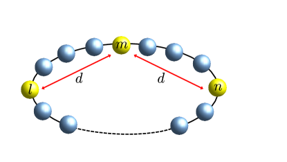
as depicted in Fig. 1. In Eq. (3), stands for the strength of the defects, and is the relative distance between them that we assume to be much smaller than the size of the system, i.e. . The Hamiltonian in Eq. (1) holds several symmetry properties. However, for our purposes, it is worth noting that possesses a -symmetry, implying that the total magnetization along the -axis is conserved, i.e. .
Regardless of the presence of defects, the model in Eq. (1) can be mapped into a quadratic Hamiltonian of spinless fermions, with annihilation and creation operators given, respectively, by , via the Jordan-Wigner transformation [29],
| (4) |
Here, stands for the parity operator along with eigenvalues . Hence, depending on the total magnetization of the state, it induces antiperiodic or periodic boundary conditions [30, 31]. In the following, we will consider only the positive parity subspace as the RDM of the three defects whose entanglement properties we investigate are equivalent to .
Because of its quadratic nature, the Hamiltonian in Eq.(II) is readily diagonalized as
| (5) |
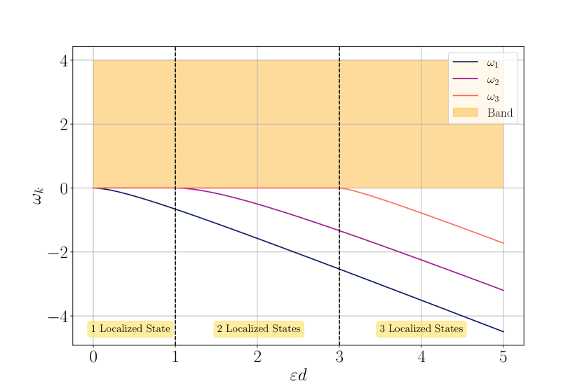
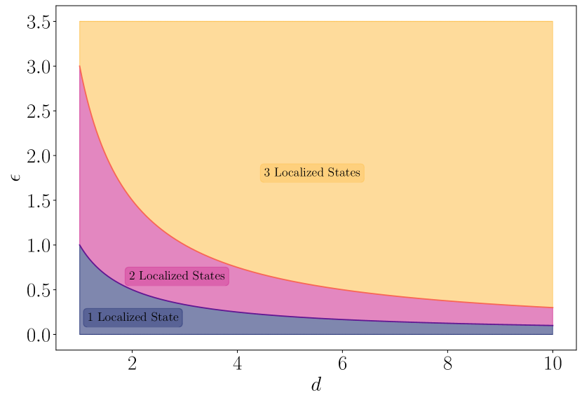
where and are, respectively, the single-particle eigenenergies and eigenstates of the fermionic problem. In the limit we recover and, in the thermodynamic limit, the single-particle spectrum makes up a continuous band with with the eigenstates encoding plane waves [32]. In contrast, taking into account a strictly positive value of , up to three discrete energy levels emerge from below the band. Using a Green’s function approach [33], it is possible to analytically determine the boundaries between the regions with one, two, or three discrete eigenstates of the Hamiltonian. Those regions are:
| one discrete energy level; | (6a) | |||
| two discrete energy levels; | (6b) | |||
| three discrete energy levels. | (6c) | |||
Details of the derivation of these results can be found in Appendix A. In Fig. 2 we show the energy spectrum of the fermionic Hamiltonian in Eq. (II), with and , as a function of the product , where it is possible to have the emergence of discrete single-particle energies. Changing , the single-particle energy spectrum is shifted vertically. Differently from the ones in the band, the eigenstates corresponding to the discrete eigenenergies are exponentially localized on the defects [34]. In contrast, the continuous energy band gets distorted and their eigenstates acquire a contribution describing back-scattering at the impurity sites [33, 35]. From Eq. (6) it is possible to identify three different regions in the plane, each one of them characterized by a different number of localized states. These regions have been depicted in Fig. 3.
III Multipartite entanglement
As already mentioned, the main goal of this work is to study the multipartite entanglement in the ground state of the model in Eq. (1) between the spins on which magnetic defects are present. Toward this end, we first need to evaluate the RDM that is obtained by tracing out all the degrees of freedom associated with the spins on which no defects are present. The form of this matrix will take into account all the symmetries of the state from which it is obtained. In our case, it is well known that the ground state of the XX model with periodic boundary conditions, as in Eq. (2), has a vanishing momentum that implies that the RDM is real [31]. This result remains unaffected by the presence of defects. Moreover, since the distance between the first and second defect, and that between the second and the third are equal, there is a reflection symmetry with respect to the central defect. Furthermore, the Hamiltonian in Eq. (1) preserves the global magnetization and therefore all its eigenstates, including the ground-state, have a well-determined value of total magnetization. Taking into account all these properties the RDM in the computational basis becomes equal to
| (7) |
This matrix is, in general, a rank-8 density matrix that can be decomposed as follows:
| (8) |
where and are, respectively, the generalized - and the generalized spin-flipped -state
| (9) | ||||
| (10) |
This decomposition is particularly useful since it allows us to prove that the three-tangle [36] of vanishes, i.e., . Such a result follows straightforwardly from the convex-roof extension of to mixed states [37] and from the well-known results that for a generalized -state, is identically zero. This restricts the possibility of genuine multipartite entanglement to -type [38], which has , but finite GME-concurrence [28]. The GME concurrence for pure states is defined as
| (11) |
where is the RDM of the th bipartition. For mixed states, similar to the three-tangle, the GME concurrence can be calculated by exploiting the convex-roof extension
| (12) |
such that and the minimization procedure is carried out over all possible pure state decompositions of .
The computation of the GME concurrence for the case of more than one localized state (that is when the rank of the density matrix is equal or larger than two) is a highly non-trivial problem, which makes the analytical solution challenging to obtain. Consequently, we resort to numerical techniques to determine a lower bound for the GME concurrence exploiting two different methods; one presented by Ma et al. [28]; and the second by Hong et al. [39]. Both algorithms were embedded within a Monte Carlo algorithm using 100 runs with random initial states with the global minimum taken to be the one with the highest GME concurrence. The BFGS [40] optimizer was employed as the local optimizer, taken from the SciPy library [41].
To complement the previous method, we also consider a separability criterion for the density matrix resorting to the algorithm presented by Hofmann et al. [42], which iteratively attempts to decompose a given density matrix into a convex sum of biseparable components. At iteration , the density matrix is expressed as the convex sum of terms , where is a biseparable state, and an additional semidefinite matrix . If, for a certain , the condition
| (13) |
is satisfied, the density matrix is separable with respect to some bipartition (see Gurvits and Barnum [43] for further details). The data is obtained by considering iterations with randomly generated biseparable states for each iteration.
Together with the multipartite entanglement, to have a complete characterization of , we also have to evaluate the bipartite entanglement between each pair of spins. Such entanglement can easily be quantified by the concurrence [44]. Due to the symmetry in the model, the concurrence between the first and the second must be equal to the one from the second and the third, i.e. . Since the partial trace of with respect to any qubit is an X-state (that is, the RDM is zero excepts along the two diagonals), we can determine the concurrence via the simplified expression provided by Amico et al. [45]. Accordingly, the concurrence between the first and second defect (and similarly between the second a third defect) is equal to
| (14) |
while concurrence between the first and third defect is equal to
| (15) |
IV Long-distance GME concurrence
As discussed in Sec. II, the XX model in Eq. (2) exhibits two distinct thermodynamic phases, a gapless one for and a gapped one for . Therefore, it is natural to study the emergence of multipartite entanglement following the presence of defects in the two regions separately.
IV.1 The paramagnetic phase
For , discrete eigenstates emerge from below the continuous band for any (see Fig. 2). For , only one discrete energy level is present. As a consequence, the reduced density matrix can be written as,
| (16) |
which is of rank 2. This case is of particular interest since we can analytically determine the GME concurrence following the path depicted in Refs. [46, 47]. We start by analyzing the GME concurrence of the family of pure states
| (17) |
where and , can be considered free parameters. Using Eq. (11), and recalling the expression of the generalized W-state in Eq. (9) the GME concurrence of these states are
| (18) |
As a result, the zero polytope [48] of the states in Eq. (IV.1) is a trivial one, where , assuming . The next step is to construct the convex characteristic curve [48]. Since , then is monotonically increasing with , and invariant with respect to . Moreover, is also linearly increasing with , which implies that it is already convex. As a result, the GME concurrence is equal to the weight of the generalized state, similar to how the concurrence between a Bell state and an unentangled state is equal to the weight of the Bell state [49]. Therefore
| (19) |
In our case, due to the symmetry properties of our system, is equal to and , with . Thus, the GME concurrence reduces to
| (20) |
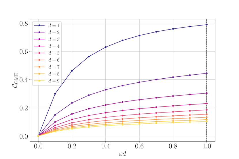
It has to be noted that, due to the range of values of , always has a non-zero GME concurrence independently of the distance , although it becomes vanishingly small as the distance increases. This dependence on the distance can be appreciated in Fig. 4 where we show the GME concurrence as a function of the rescaled defects’ intensity in the region with a single localized energy eigenstate.
For , more localized states appear in the ground state of the system, and the rank of the RDM increases. This makes finding the convex-roof extension via analytical methods as done above for rank-2 density matrices highly non-trivial. Therefore, in the following, we resort to the numerical methods described in the previous section to determine the lower bound of the GME concurrence and corroborate our results via evaluating the separability criterion Eq. (13) of genuine multipartite entanglement.
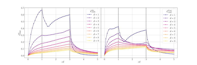
Fig. 5 shows the lower bound of the GME concurrence for as a function of . For completeness, we compute this bound also for the previous case of only one localized eigenstate (). We notice that, although the lower bounds of the GME concurrence decrease as the defects’ separation increases, they remain finite indicating that long-distance GME concurrence is attainable for every value of and . Hence the numerically derived bounds for confirm the presence of GME concurrence when multiple localized states contribute to the ground state. To strengthen these findings, we also consider the separability criterion Eq. (13), which complements the GME results (Fig. 7). We always found , that is, the state is not separable for any bipartition. Finally, we also used the separability criterion based on the Hilbert-Schmidt distance developed in Ref. [50] and strong numerical evidence suggests a non-zero distance to the closest bi-separable state. These results emphasize the ability of the defects to sustain long-distance multipartite entanglement that would otherwise be absent in uniform systems.
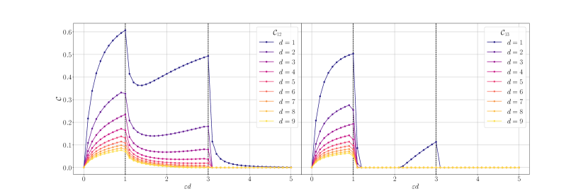
In Fig. 6 we show the concurrence between the defects as evaluated via Eq. (14) and (15). While the concurrence between adjacent defects and is nonzero for smaller , it vanishes beyond and . Similarly, the concurrence between the outer defects is negligible for most of the parameter space. As a consequence, density matrices of the form of Eq. (7) can sustain states with non-zero GME concurrence and vanishing two-qubit concurrence, similarly to -type states [51].
IV.2 The critical phase
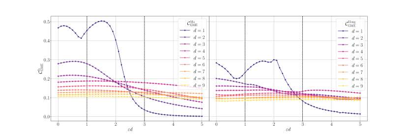
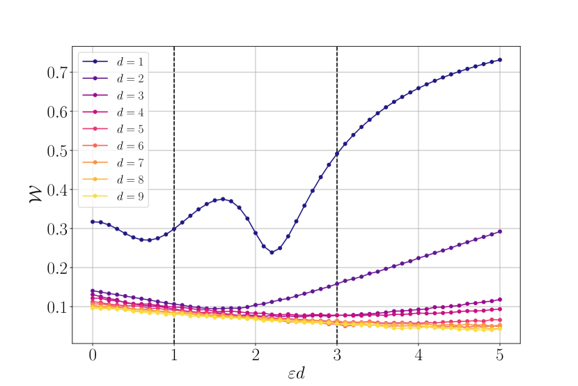
For any , regardless of the value of , the RDM is always of rank 8, preventing an analytical determination of the GME concurrence. However, similar to Sec. IV.1 above, we report the two lower bounds presented by Ma et al. [28] and Hong et al. [39], the respective concurrences and , as well as the separability criterion in Eq. (13). Fig. 8 shows the lower bounds for the GME concurrence and Fig. 9 the separability witness for . Similarly to the case of , non-zero long-distance entanglement is present for any value of also in the absence of any pairwise concurrence between the qubits, which vanishes for and .
V Conclusion
In this work, we studied the interplay between magnetic defects and multipartite entanglement in an XX spin- chain subjected to a transverse field. Using analytical techniques complemented by numerical methods, we characterized the emergence of localized bound states at the defect sites.
Our findings demonstrate the existence of regions in parameter space, defined by the defect intensity and separation, where GME arises. For a single localized state, the GME concurrence was derived analytically. When multiple localized states are present, numerical approaches were employed to establish lower bounds on GME concurrence and validate multipartite entanglement through separability witnesses.
Interestingly, while pairwise entanglement between defects vanishes in certain regions, the GME concurrence persists, underscoring the robustness of multipartite entanglement at larger defect separations. This allows for the generation of long-distance multipartite entanglement in many-body system with nearest-neighbor interaction by the application of local magnetic defects at desired locations. This approach to the generation of multipartite entanglement appears, simultaneously, easier and more flexible than the one based on models with Cluster interactions [52, 53] hence disclosing the way of possible technological applications in quantum communication and quantum technologies. Apart from such applications, our analytic results and numerical lower bounds shed light on the properties of multipartite entanglement in density matrices without coherence between different magnetization sectors, where only -type entanglement can be present.
Although we restricted our analysis to three defects, the proposed method for long-distance multipartite entanglement generation via local magnetic fields can be straightforwardly extended to a higher number of defects to investigate higher SLOCC entanglement classes [6] or to the XY model, which sustains GHZ-type entanglement [19].
Acknowledgements.
MC acknowledges funding by the Tertiary Education Scholarships Scheme MFED 758/2021/34. MC and TJGA acknowledge Xjenza Malta for their support via the project GROUNDS IPAS-2023-059. JO acknowledges the support by the PNRR MUR Project No. PE0000023-NQSTI, and thanks Viktor Eisler for useful discussions. RB acknowledges support from the Croatian Science Foundation (HrZZ) Project No. IP-2019-4-3321 and Austrian Science Fund (FWF) Grant-DOI:10.55776/P35434. MW acknowledges the support by NCN (Poland) Grant 2017/26/E/ST2/01008.Appendix A Green functions method
We consider the tight-binding Hamiltonian in the presence of three impurities, corresponding to the one in Eq.(II), decomposed as
| (21) |
where is the tight-binding Hamiltonian without impurities, characterized by nearest-neighbor interactions
| (22) |
and denotes the perturbation, that is assumed to be diagonal,
| (23) |
We introduce the unperturbed Green operator corresponding to ,
| (24) |
In the limit , the set of states form a continuous band with energies . The matrix elements of between two localized states are given by
| (25) |
and
| (26) |
where . The full Green operator , corresponding to the full Hamiltonian , can be obtained as
| (27) |
where the -matrix is determined from the knowledge of and , as
| (28) |
The -matrix can be obtained following the approach in [33]. Introducing the unit operator into Eq.(28), we get
| (29) |
Since the defects are diagonal, we need to retain in the summation only the terms , that can be written as scalar product , with
| (30) |
With this notation, we have
| (31) |
where
| (32) | ||||
| (33) |
The first step is to invert the matrix
| (34) |
The determinant gives
| (35) |
where we define as
| (36) |
and
| (37) |
The poles of the Green functions for the three-defects problem can be determined from the zeroes of Eq. (A). In the case and , that is, the intensity of the magnetic field on the three defects is the same and the defects are symmetrically placed around the central defect, as in Fig. 2 of the main paper, we find, using the Mathematica software package and confirmed through numerical simulations, that for only one solution is found, for two solutions are found, and for , three solutions are found, as reported in Eqs. (6) in the main paper.
The emergence of three localized states can also be obtained by solving the 1D Schrodinger equation with three delta potentials:
| (38) |
where the potential is
| (39) |
Straightforward calculations give that the solutions for bound states of this problem are given as:
| 1 even solution: | (40a) | |||
| 1 odd and 1 even solution: | (40b) | |||
| 1 odd and 2 even solutions: | (40c) | |||
and by setting , we obtain Eqs. (6).
References
- Epping et al. [2017] M. Epping, H. Kampermann, C. Macchiavello, and D. Bruß, New Journal of Physics 19, 10.1088/1367-2630/aa8487 (2017), arxiv:1612.05585 .
- Yeo and Chua [2006] Y. Yeo and W. Chua, Physical Review Letters 96, 060502 (2006).
- Tóth [2012] G. Tóth, Phys. Rev. A 85, 022322 (2012).
- Raussendorf and Briegel [2001] R. Raussendorf and H. J. Briegel, Phys. Rev. Lett. 86, 5188 (2001).
- Dür et al. [2000] W. Dür, G. Vidal, and J. I. Cirac, Physical Review A 62, 062314 (2000).
- Verstraete et al. [2002] F. Verstraete, J. Dehaene, B. De Moor, and H. Verschelde, Phys. Rev. A 65, 052112 (2002).
- Horodecki et al. [2024] P. Horodecki, L. Rudnicki, and K. Życzkowski, Multipartite entanglement (2024), arXiv:2409.04566 [quant-ph] .
- Ma et al. [2024] M. Ma, Y. Li, and J. Shang, Fundamental Research https://doi.org/10.1016/j.fmre.2024.03.031 (2024).
- Walter et al. [2016] M. Walter, D. Gross, and J. Eisert, Multipartite Entanglement, in Quantum Information (John Wiley & Sons, Ltd, 2016) Chap. 14, pp. 293–330.
- Eltschka and Siewert [2014] C. Eltschka and J. Siewert, Journal of Physics A: Mathematical and Theoretical 47, 424005 (2014).
- Bengtsson and Życzkowski [2017] I. Bengtsson and K. Życzkowski, Geometry of Quantum States (Cambridge University Press, Cambridge, 2017).
- Lepori et al. [2023] L. Lepori, A. Trombettoni, D. Giuliano, J. Kombe, J. Yago Malo, A. J. Daley, A. Smerzi, and M. Luisa Chiofalo, Journal of Physics A: Mathematical and Theoretical 56, 305302 (2023).
- Wieśniak [2024] M. Wieśniak, Multipartite Entanglement versus Multiparticle Entanglement (2024), arXiv:2407.13348 [quant-ph] .
- Jungnitsch et al. [2011] B. Jungnitsch, T. Moroder, and O. Gühne, Phys. Rev. Lett. 106, 190502 (2011).
- Cianciaruso et al. [2016] M. Cianciaruso, T. R. Bromley, and G. Adesso, npj Quantum Information 2, 16030 (2016).
- Sperling and Vogel [2013] J. Sperling and W. Vogel, Phys. Rev. Lett. 111, 110503 (2013).
- Gühne et al. [2005] O. Gühne, G. Tóth, and H. J. Briegel, New Journal of Physics 7, 229 (2005).
- Amico et al. [2008] L. Amico, R. Fazio, A. Osterloh, and V. Vedral, Reviews of Modern Physics 80, 517 (2008).
- Giampaolo and Hiesmayr [2013] S. M. Giampaolo and B. C. Hiesmayr, Phys. Rev. A 88, 052305 (2013).
- Liu et al. [2022] Z. Liu, Y. Tang, H. Dai, P. Liu, S. Chen, et al., Phys. Rev. Lett. 129, 260501 (2022).
- Campos Venuti et al. [2006] L. Campos Venuti, C. Degli Esposti Boschi, and M. Roncaglia, Phys. Rev. Lett. 96, 247206 (2006).
- Giampaolo and Illuminati [2009] S. M. Giampaolo and F. Illuminati, Phys. Rev. A 80, 050301 (2009).
- Campos Venuti et al. [2007] L. Campos Venuti, S. M. Giampaolo, F. Illuminati, and P. Zanardi, Phys. Rev. A 76, 052328 (2007).
- Giampaolo and Illuminati [2010] S. M. Giampaolo and F. Illuminati, New Journal of Physics 12, 025019 (2010).
- Apollaro and Plastina [2006] T. J. G. Apollaro and F. Plastina, Phys. Rev. A 74, 062316 (2006).
- Plastina and Apollaro [2007] F. Plastina and T. J. G. Apollaro, Phys. Rev. Lett. 99, 177210 (2007).
- Apollaro et al. [2008a] T. Apollaro, A. Cuccoli, A. Fubini, F. Plastina, and P. Verrucchi, Physical Review A 77, 062314 (2008a).
- Ma et al. [2011] Z.-H. Ma, Z.-H. Chen, J.-L. Chen, C. Spengler, A. Gabriel, et al., Physical Review A 83, 062325 (2011), arXiv:1101.2001 .
- Lieb et al. [1961] E. Lieb, T. Schultz, and D. Mattis, Annals of Physics 16, 407 (1961).
- Damski and Rams [2014] B. Damski and M. M. Rams, Journal of Physics A: Mathematical and Theoretical 47, 025303 (2014).
- Franchini [2017] F. Franchini, An Introduction to Integrable Techniques for One-Dimensional Quantum Systems, Vol. 940 (Springer International Publishing, Cham, 2017) arxiv:1609.02100 .
- De Pasquale et al. [2008] A. De Pasquale, G. Costantini, P. Facchi, G. Florio, S. Pascazio, et al., The European Physical Journal Special Topics 160, 127 (2008).
- Economou [2006] E. N. Economou, Green’s Functions in Quantum Physics, 3rd ed., Springer Series in Solid-State Sciences (Springer-Verlag Berlin Heidelberg, 2006).
- Anderson [1958] P. W. Anderson, Phys. Rev. 109, 1492 (1958).
- Apollaro et al. [2008b] T. J. G. Apollaro, A. Cuccoli, A. Fubini, F. Plastina, and P. Verrucchi, International Journal of Quantum Information 06, 567 (2008b).
- Coffman et al. [1999] V. Coffman, J. Kundu, and W. K. Wootters, Physical Review A 61, 052306 (1999), arXiv:9907047 [quant-ph] .
- Horodecki et al. [2009] R. Horodecki, P. Horodecki, M. Horodecki, and K. Horodecki, Reviews of Modern Physics 81, 865 (2009).
- Acín et al. [2001] A. Acín, D. Bruß, M. Lewenstein, and A. Sanpera, Physical Review Letters 87, 040401 (2001).
- Hong et al. [2012] Y. Hong, T. Gao, and F. Yan, Phys. Rev. A 86, 062323 (2012).
- Nocedal and Wright [2006] J. Nocedal and S. J. Wright, Numerical Optimization, 2nd ed. (Springer, New York, NY, USA, 2006).
- Virtanen et al. [2020] P. Virtanen, R. Gommers, T. E. Oliphant, M. Haberland, T. Reddy, et al., Nature Methods 17, 261 (2020).
- Hofmann et al. [2014] M. Hofmann, A. Osterloh, and O. Gühne, Phys. Rev. B 89, 134101 (2014).
- Gurvits and Barnum [2002] L. Gurvits and H. Barnum, Phys. Rev. A 66, 062311 (2002).
- Wootters [1998] W. K. Wootters, Phys. Rev. Lett. 80, 2245 (1998).
- Amico et al. [2004] L. Amico, A. Osterloh, F. Plastina, R. Fazio, and G. Massimo Palma, Phys. Rev. A 69, 022304 (2004).
- Lohmayer et al. [2006] R. Lohmayer, A. Osterloh, J. Siewert, and A. Uhlmann, Phys. Rev. Lett. 97, 260502 (2006).
- Eltschka et al. [2008] C. Eltschka, A. Osterloh, J. Siewert, and A. Uhlmann, New Journal of Physics 10, 043014 (2008).
- Osterloh et al. [2008] A. Osterloh, J. Siewert, and A. Uhlmann, Phys. Rev. A 77, 032310 (2008).
- Abouraddy et al. [2001] A. F. Abouraddy, B. E. A. Saleh, A. V. Sergienko, and M. C. Teich, Phys. Rev. A 64, 050101 (2001).
- Pandya et al. [2020] P. Pandya, O. Sakarya, and M. Wieśniak, Phys. Rev. A 102, 012409 (2020).
- Hashemi Rafsanjani et al. [2012] S. M. Hashemi Rafsanjani, M. Huber, C. J. Broadbent, and J. H. Eberly, Phys. Rev. A 86, 062303 (2012).
- Giampaolo and Hiesmayr [2014] S. M. Giampaolo and B. C. Hiesmayr, New Journal of Physics 16, 093033 (2014).
- Giampaolo and Hiesmayr [2015] S. M. Giampaolo and B. C. Hiesmayr, Phys. Rev. A 92, 012306 (2015).