Symmetric Cartan calculus,
the Patterson-Walker metric
and symmetric cohomology

Abstract.

We develop symmetric Cartan calculus, an analogue of classical Cartan calculus for symmetric differential forms. We first show that the analogue of the exterior derivative, the symmetric derivative, is not unique and its different choices are parametrized by torsion-free affine connections. We use a choice of symmetric derivative to generate the symmetric bracket and the symmetric Lie derivative, and give geometric interpretations of all of them. By proving the structural identities and describing the role of affine morphisms, we reveal an unexpected link of symmetric Cartan calculus with the Patterson-Walker metric, which we recast as a direct analogue of the canonical symplectic form on the cotangent bundle. We show that, in the light of the Patterson-Walker metric, symmetric Cartan calculus becomes a complete analogue of classical Cartan calculus. As an application of this new framework, we introduce symmetric cohomology, which involves Killing tensors, or, in the case of the Levi-Civita connection, Killing vector fields. We finish by characterizing the Levi-Civita connections of $\mathrm{S}^{1}$ in terms of symmetric cohomology.

1. Introduction

Classical Cartan calculus, understood as the calculus of vector fields $\mathfrak{X}(M)$ and differential forms $\Omega^{\bullet}(M)$ on a manifold $M$, is an ubiquitous language for differential geometry. Its structural identities are the graded commutators of the contraction operator $\iota$, the exterior derivative $d$ and the Lie derivative $L$. Namely, for $X,Y\in\mathfrak{X}(M)$, we have:

(1) $${}_{\text{g}} =0, [\mathrm{d},\mathrm{d}]_{\text{g}} =0, [\iota_{X},\mathrm{d}]_{\text{g}} =L_{X},$$

$$[L_{X},\iota_{Y}]_{\text{g}} =\iota_{[X,Y]}, [L_{X},L_{Y}]_{\text{g}} =L_{[X,Y]}, [\mathrm{d},L_{X}]_{\text{g}} =0.$$

The exterior derivative plays a geometric generating role. Together with the contraction, which is a linear-algebraic operation (that is, at the level of bundles, not necessarily sections), it recovers the Lie derivative and also the Lie bracket as a derived bracket. Furthermore, the exterior derivative gives rise to the de Rham cohomology.

A very natural question is whether there is an analogous framework for symmetric differential forms and what it might be helpful for. This would first mean finding analogues to the exterior derivative, the Lie derivative and the Lie bracket satisfying similar properties. Surprisingly, the only precedent we are aware of is the definition of a symmetric bracket in [9] (later geometrically interpreted in [17]), which was used, by mimicking the explicit formulas in the usual setting, to define a symmetric differential and a symmetric Lie derivative [13]. We have found no justification that these are the only possible or even reasonable choices, no exhaustive study of the structural identities analogous to (1) and, beyond the symmetric bracket [2, 5], neither a full geometric interpretation nor a significant application.

The aim of the present work is to develop and justify a sound and geometrically meaningful approach to symmetric Cartan calculus, as well as to show its two-way interaction with the Patterson-Walker metric, and introduce a symmetric cohomology theory, which is related to Killing tensors. Key to our strategy is our starting point: we look for all possible symmetric analogues of the exterior derivative that can play an equivalent generating role as a geometric derivation (Definition 2.4).

The first main feature of symmetric Cartan calculus is, precisely, that there is no canonical symmetric derivative for symmetric differential forms, which we denote by $\Upsilon^{\bullet}(M)$. Such an analogue depends on the choice of a connection, which can be, without loss of generality, assumed to be torsion free. In fact, we prove:

Proposition 2.9.

The map $\nabla\mapsto\nabla^{s}$ gives an isomorphism of $\Upsilon^{2}(M,TM)$-affine spaces:

$$\left\{\begin{array}[]{c}\text{torsion-free}\\ \text{connections on }M\end{array}\right\}\overset{\sim}{\longleftrightarrow}\left\{\begin{array}[]{c}\text{geometric derivations of the algebra}\\ \text{of symmetric forms on }M\end{array}\right\}.$$

An a priori surprising fact is that $\nabla^{s}$ does not square to zero. However, this is natural, since the symmetric derivative is a usual derivation and derivations are an algebra for the usual commutator, as opposed to the graded commutator for graded derivations. Thus, squaring to zero is natural in the context of classical Cartan calculus since $[\mathrm{d},\mathrm{d}]_{g}=2\,\mathrm{d}\circ\mathrm{d}$, whereas in the symmetric case, we have that the analogous expression of squaring to zero is $[\nabla^{s},\nabla^{s}]=0$ for the usual commutator, which is trivially satisfied.

We give a geometric interpretation of $\nabla^{s}$ making use of the correspondence between a symmetric form $\varphi$ and a polynomial in velocities $\tilde{\varphi}$ (an element of a subspace of $\mathcal{C}^{\infty}(M)$, as we explain in Section 2.3), together with the geodesic spray $X_{\nabla}\in\mathfrak{X}(TM)$.

Proposition 2.13.

Let $\nabla$ be a connection on $M$. For every $\varphi\in\Upsilon^{r}(M)$ we have

$$\widetilde{\nabla^{s}\varphi}=X_{\nabla}\tilde{\varphi}.$$

The symmetric Lie derivative with respect to a vector field $X\in\mathfrak{X}(M)$ is introduced as $L_{X}^{s}=[\iota_{X},\nabla^{s}]$ and we show in Proposition 2.18 (see also Figure 1) that it captures the variation with respect to a combination of the flow of $X$ and the parallel transport with respect to $\nabla$. Finally, the symmetric bracket is derived from the formula $[L^{s}_{X},\iota_{Y}]=\iota_{\langle X:Y\rangle_{s}}$. Its geometric interpretation in relation to geodesically invariant distributions is recalled in Section 2.7. Overall, we have the following properties for the (ungraded) commutator:

$$[\iota_{X},\iota_{Y}] =0, [\nabla^{s},\nabla^{s}] =0, [\iota_{X},\nabla^{s}] =L^{s}_{X},$$

$$[L^{s}_{X},\iota_{Y}] =\iota_{\langle X:Y\rangle_{s}}, [L^{s}_{X},L^{s}_{Y}] \neq L^{s}_{\langle X:Y\rangle_{s}} [\nabla^{s},L^{s}_{X}] \neq 0.$$

Note that the analogues of the last two formulae of (1) are not true. Instead, we show in Section 3 that

$$[L^{s}_{X},L^{s}_{Y}] =L^{s}_{[X,Y]}+\iota^{s}_{2(\nabla_{\nabla X}Y-\nabla_{\nabla Y}X-R_{\nabla}(X,Y))},$$

$$[\nabla^{s},L^{s}_{X}] =2\nabla^{s}_{\nabla X}+\iota^{s}_{2\operatorname{sym}\iota_{X}R_{\nabla}+R^{s}_{\nabla}X}.$$

The study of the right-hand side of these expressions leads us to find an unexpected link with the Patterson-Walker metric $g_{\nabla}$, a metric on $T^{*}M$ that is determined by the choice of a torsion-free connection $\nabla$ on $M$. On the one hand, by using a lift $\hat{\nabla}$ of the connection $\nabla$ to $T^{*}M$ (Section 5.2), the symmetric derivative allows us to recast the Patterson-Walker metric as an analogue of the canonical symplectic form on $T^{*}M$.

Theorem 5.7.

For any torsion-free connection $\nabla$ on $M$, there holds

$$\hat{\nabla}^{s}\alpha_{\text{can}}=g_{\nabla},$$

where $\alpha_{\text{can}}$ is the canonical $1$-form on $T^{*}M$.

On the other hand, the Patterson-Walker metric, together with the notion of the complete lift $X^{c}\in\mathfrak{X}(T^{*}M)$ of a vector field $X$, gives a framework in which the structural identities become much simpler.

Theorem 5.19.

Let $\nabla$ be a torsion-free connection on $M$ and $X,Y\in\mathfrak{X}(M)$. All of the six relations

$$[\iota_{X},\iota_{Y}] =0, [\nabla^{s},\nabla^{s}] =0, [\iota_{X},\nabla^{s}] =L^{s}_{X},$$

$$[L^{s}_{X},\iota_{Y}] =\iota_{\langle X:Y\rangle_{s}}, [L^{s}_{X},L^{s}_{Y}] =0, [\nabla^{s},L^{s}_{X}] =0$$

are satisfied if and only if $X^{\text{c}}$ and $Y^{\text{c}}$ are gradient Killing vector fields for $g_{\nabla}$.

This seemingly extra condition on $X$ and $Y$ implicitly appears in the classical case as well. Indeed, the analogues of gradient Killing vector fields for $g_{\nabla}$ are Hamiltonian ones for the canonical $2$-form $\omega_{\text{can}}$, and complete lifts are always Hamiltonian. This, together with the fact that $[L^{s}_{X},L^{s}_{Y}]=0=L^{s}_{\langle X:Y\rangle}$ if $X^{c}$ and $Y^{c}$ are gradient Killing, draws a complete analogy between Theorem 5.19 and (1).

The study of the lifts required to prove these last two theorems is recalled in Appendix B.

Finally, just as the exterior derivative plays a generating role in classical Cartan calculus and is the basis of de Rham cohomology, the question of whether there is any cohomology theory associated to the symmetric derivative arises naturally.

Closed symmetric forms for the symmetric derivative $\nabla^{s}$ recover the notion of Killing tensors. In the case of the Levi-Civita connection of a (pseudo-)Riemannian metric, Killing tensors are well established. They are related to the separability of Hamilton-Jacobi equation [3], or the symmetries of the Laplacian [10]. Probably the most famous Killing tensor is the Carter tensor in the Kerr-Newman spacetime, the spacetime of a charged rotating black hole [6, 7, 22].

Defining a cohomology theory with an operator that does not square to zero requires some adjustment, namely, considering the intersection of the image with the kernel. We do this to define symmetric cohomology, and give a geometric interpretation in terms of polynomials in velocities (Corollary 6.14). We focus specially on the first symmetric cohomology group. We prove that its dimension is bounded, and, when dealing with a (pseudo-)Riemannian metric, we can relate it to Killing vector fields modulo gradient Killing vector fields.

Symmetric cohomology depends, as symmetric Cartan calculus does, on the choice of a torsion-free connection. Far from being a hindrance, we take advantage of this fact, to prove our last result, which offers a characterization of Levi-Civita connections on $\mathrm{S}^{1}$ in terms of symmetric cohomology.

Proposition 6.25.

The only connections $\nabla$ on $\mathrm{S}^{1}$ such that $H^{1}_{\nabla}(\mathrm{S}^{1})\neq\{0\}$ (and hence ${\mathbb{R}}$) are the Levi-Civita connections for any choice of metric on $\mathrm{S}^{1}$.

Further applications of symmetric Cartan calculus will come in forthcoming papers about symmetric Poisson structures and generalized geometry.

We finish the paper with a table (Appendix D) that summarizes and compares various aspects of symmetric Cartan calculus with classical Cartan calculus.

Acknowledgements. We would like to thank the Weizmann Institute of Science for their hospitality in hosting us as visitors, Andrew Lewis for helpful discussions about the symmetric bracket and Rudolf Šmolka for noticing a mistake in the first version of this text.

Notation and conventions. We work on the smooth category for manifolds and maps. We denote an arbitrary manifold (of positive dimension) by $M$, its smooth functions by $\mathcal{C}^{\infty}(M)$, its tangent bundle by $TM$, its cotangent bundle by $T^{*}M$, its vector fields by $\mathfrak{X}(M)$ and its differential forms by $\Omega^{\bullet}(M)$.

When we consider a connection on $M$, we mean an affine connection (that is, a connection on $TM$), which can determine other connections (for instance, on $T^{*}M$ by duality). We will denote these connections with the same symbol.

When we consider a vector space $V$, we mean a finite-dimensional vector space over ${\mathbb{R}}$ or ${\mathbb{C}}$. We use the Einstein summation convention throughout the text.

Note that our definition of symmetric cohomology will be unrelated to that of symmetric group cohomology introduced in [20].

2. Symmetric Cartan calculus

We first look at the linear-algebraic level before moving to smooth manifolds.

2.1. The symmetric algebra and its derivations

Consider a vector space $V$, its dual space $V^{*}$ and the tensor algebra $\otimes^{\bullet}V^{*}$. The natural action of a permutation $\pi\in\mathcal{S}_{r}$ on a decomposable element (with $\alpha^{j}\in V^{*}$),

$$\pi\cdot(\alpha^{1}\otimes\ldots\otimes\alpha^{r}):=\alpha^{\pi 1}\otimes\ldots\otimes\alpha^{\pi r},$$

is extended linearly to $\otimes^{r}V^{*}$ and gives rise to the symmetric projection $\operatorname{sym}_{r}:\otimes^{r}V^{*}\rightarrow\otimes^{r}V^{*}$,

$$\operatorname{sym}_{r}(\varphi):=\frac{1}{r!}\sum_{\pi\in\mathcal{S}_{r}}\pi\cdot\varphi,$$

and, more generally, $\operatorname{sym}:=\oplus_{r\in{\mathbb{N}}}\operatorname{sym}_{r}$. Consider the ${\mathbb{N}}$-graded vector space

$$\operatorname{Sym}^{\bullet}V^{*}:=\frac{\otimes^{\bullet}V^{*}}{\ker\operatorname{sym}}\cong\operatorname{Im}\operatorname{sym}.$$

The latter isomorphism allows us to realize $\operatorname{Sym}^{\bullet}V^{*}$ as a vector subspace of $\otimes^{\bullet}V^{*}$. Define the symmetric product of $\varphi\in\operatorname{Sym}^{r}V^{*}$ and $\psi\in\operatorname{Sym}^{l}V^{*}$ by

$$\varphi\odot\psi:=\frac{(r+l)!}{r!\,l!}\operatorname{sym}(\varphi\otimes\psi).$$

We thus have the symmetric algebra $(\operatorname{Sym}^{\bullet}V^{*},+,\odot)$.

At this linear-algebraic level, we can already look at the contraction operator. The degree-$(-1)$ map $\iota_{X}$, for any $X\in V$, descends from $\otimes^{\bullet}V^{*}$ to $\operatorname{Sym}^{\bullet}V^{*}$, where it becomes a derivation, that is,

(2) $$\iota_{X}(\varphi\odot\psi)=\iota_{X}\varphi\odot\psi+\varphi\odot\iota_{X}\psi,$$

as we show in the proof of the next lemma. Note that the sign is always $+$, that is, it is not graded.

Lemma 2.1.

The degree-$(-1)$ derivations of $\operatorname{Sym}^{\bullet}V^{*}$ are in bijective correspondence with $V$ via the contraction operator $\iota$.

Proof.

We first prove that the contraction operator is indeed a derivation of $\operatorname{Sym}^{\bullet}V^{*}$. Given $\varphi\in\operatorname{Sym}^{r}V^{*}$ and $\psi\in\operatorname{Sym}^{l}V^{*}$, we denote $n:=r+l-1$. We shall use the shorthand notation $\varphi(Y):=\varphi(Y,\makebox[10.00002pt][c]{.\hfil.\hfil.},Y)$ for a symmetric $r$-tensor $\varphi$ acting on $r$ copies of a vector $Y\in V$. Then, for all $Y\in V$,

$$(\iota_{X}(\varphi\odot\psi))(Y)=\frac{1}{r!l!}\sum_{\pi\in\mathcal{S}_{n}}\iota_{X}(\pi\cdot(\varphi\otimes\psi))(Y).$$

We can write the symmetric group $\mathcal{S}_{n}$ as the disjoint union of the two subsets $\mathcal{S}^{r}_{n}:=\{\pi\in\mathcal{S}_{n}\,|\,1\in\pi(\{1,\makebox[10.00002pt][c]{.\hfil.\hfil.},r\})\}$ and $\mathcal{S}^{l}_{n}:=\{\pi\in\mathcal{S}_{n}\,|\,1\in\pi(\{r+1,\makebox[10.00002pt][c]{.\hfil.\hfil.},r+l\})\}$. Therefore,

$$(\iota_{X}(\varphi\odot\psi))(Y)=\frac{1}{r!l!}\Big{(}\sum_{\pi\in\mathcal{S}^{r}_{n}}(\iota_{X}\varphi)(Y)\,\psi(Y)+\sum_{\pi\in\mathcal{S}^{l}_{n}}\varphi(Y)\,(\iota_{X}\psi)(Y)\Big{)}.$$

Since the cardinal of the sets $\mathcal{S}^{r}_{n}$ and $\mathcal{S}^{l}_{n}$ is $n!\,r$ and $n!\,l$, respectively, we arrive at

$$(\iota_{X}(\varphi\,\odot\,\psi))(Y) =\frac{n!}{(r-1)!l!}(\iota_{X}\varphi)(Y)\,\psi(Y)+\frac{n!}{r!(l-1)!}\,\varphi(Y)\,(\iota_{X}\psi)(Y)$$

$$=\frac{1}{(r-1)!l!}\sum_{\pi\in\mathcal{S}_{n}}(\iota_{X}\varphi)(Y)\,\psi(Y)+\frac{1}{r!(l-1)!}\sum_{\pi\in\mathcal{S}_{n}}\varphi(Y)\,(\iota_{X}\psi)(Y)$$

$$=(\iota_{X}\varphi\odot\psi+\varphi\odot\iota_{X}\psi)(Y).$$

Identity (2) then follows from polarization, so $\iota_{X}$ is a derivation. As an algebra, $\operatorname{Sym}^{\bullet}V^{*}$ is generated by $\operatorname{Sym}^{0}V^{*}$, that is, the scalars (where degree-$(-1)$ maps act trivially), and $\operatorname{Sym}^{1}V^{*}=V^{*}$, whose linear maps are exactly given by $(V^{*})^{*}\cong V$ via the contraction $\iota$. ∎

2.2. Geometric derivations

Given a manifold $M$, we replace $V$ in Section 2.1 by $T_{m}M$ and consider the $r$th-symmetric power bundle

$$\operatorname{Sym}^{r}T^{*}M,$$

whose sections we denote by $\Upsilon^{r}(M)$. We define the graded $\mathcal{C}^{\infty}(M)$-module

$$\Upsilon^{\bullet}(M):=\bigoplus_{r\in{\mathbb{N}}}\Upsilon^{r}(M).$$

Remark 2.2.

Note that $\Upsilon^{0}(M)=\mathcal{C}^{\infty}(M)$ and $\Upsilon^{1}(M)=\Omega^{1}(M)$, we will use one notation or the other depending on the context. On the other hand, we have avoided talking about $\operatorname{Sym}^{\bullet}T^{*}M$ since it would be a bundle of infinite rank.

Remark 2.3.

It will be convenient to also introduce the notation

$$\Upsilon^{r}(M,E):=\Gamma(\operatorname{Sym}^{r}T^{*}M\otimes E)$$

for an arbitrary vector bundle $E$ over $M$ and, analogously, $\Upsilon^{\bullet}(M,E)$.

The symmetric projection, the symmetric product and the contraction of Section 2.1 are easily extended to tensor fields. We thus obtain a graded algebra

$$(\Upsilon^{\bullet}(M),+,\odot).$$

The derivations of any graded algebra together with the commutator form a Lie algebra that is moreover graded. In this case, we denote it by $\operatorname{Der}(\Upsilon^{\bullet}(M)).$ For derivations of fixed degree, we will use a subindex, e.g., $\iota_{X}\in\operatorname{Der}_{-1}(\Upsilon^{\bullet}(M))$.

Since the exterior derivative, together with the contraction, generates the Cartan calculus for $\Omega^{\bullet}(M)$, now we look for analogous derivations of $\Upsilon^{\bullet}(M)$, which we call geometric.

Definition 2.4.

A geometric derivation $D\in\mathrm{Der}(\Upsilon^{\bullet}(M))$ is a derivation of degree $1$ satisfying, for all $f\in\mathcal{C}^{\infty}(M)$ and $X\in\mathfrak{X}(M)$,

$$(Df)(X)=Xf.$$

Every derivation of $\Upsilon^{\bullet}(M)$ is a local operator, and since the action on functions is prescribed, any geometric derivation is uniquely characterized by its action on $1$-forms. Namely, it is determined by a linear map $D:\Upsilon^{1}(M)\rightarrow\Upsilon^{2}(M)$ such that

(3) $$D(f\alpha)=\mathrm{d}f\odot\alpha+fD\alpha$$

for all $f\in\mathcal{C}^{\infty}(M)$ and $\alpha\in\Upsilon^{1}(M)=\Omega^{1}(M)$. Formula (3) resembles the defining property of a connection on the cotangent bundle. In fact, given such a connection $\nabla:\Omega^{1}(M)\rightarrow\Omega^{1}(M,T^{*}M)$, we define the linear map $\nabla^{s}:\Upsilon^{1}(M)\rightarrow\Upsilon^{2}(M)$ by

(4) $$\nabla^{s}:=2\operatorname{sym}\circ\,\nabla,$$

which satisfies

$$\nabla^{s}(f\alpha)=2\operatorname{sym}(\nabla(f\alpha))=2\operatorname{sym}(\mathrm{d}f\otimes\alpha+f\nabla\alpha)=\mathrm{d}f\odot\alpha+f\nabla^{s}\alpha.$$

Definition 2.5.

Let $\nabla$ be a connection on $M$. The symmetric derivative corresponding to $\nabla$ is the geometric derivation $\nabla^{s}\in\mathrm{Der}(\Upsilon^{\bullet}(M))$, defined by (4).

In fact, these are all the possible geometric derivations.

Lemma 2.6.

Every geometric derivation is the symmetric derivative corresponding to some affine connection.

Proof.

Consider an arbitrary geometric derivation $D$ and define

$$\nabla:=\frac{1}{2}\left.(D+\mathrm{d})\right|_{\Omega^{1}(M)},$$

which is a linear map $\Omega^{1}(M)\rightarrow\Omega^{1}(M,T^{*}M)$. Moreover, for all $f\in\mathcal{C}^{\infty}(M)$ and $\alpha\in\Omega^{1}(M)$,

$$\nabla(f\alpha) =\frac{1}{2}(D(f\alpha)+\mathrm{d}(f\alpha))=\frac{1}{2}(\mathrm{d}f\odot\alpha+fD\alpha+\mathrm{d}f\wedge\alpha+f\mathrm{d}\alpha)$$

$$=\frac{1}{2}(\mathrm{d}f\otimes\alpha+\alpha\otimes\mathrm{d}f+\mathrm{d}f\otimes\alpha-\alpha\otimes\mathrm{d}f)+f\nabla\alpha=\mathrm{d}f\otimes\alpha+f\nabla\alpha,$$

thus $\nabla$ is a connection. As $\mathrm{d}\alpha\in\Omega^{2}(M)$, $\operatorname{sym}(\mathrm{d}\alpha)=0$, so $\nabla^{s}=2\operatorname{sym}\circ\nabla=D$. ∎

To any connection $\nabla$ on $M$ with torsion $T_{\nabla}\in\Omega^{2}(M,TM)$ we can associate the torsion-free connection $\nabla^{0}$ given, for $X,Y\in\mathfrak{X}(M)$, by

$$\nabla^{0}_{X}Y:=\nabla_{X}Y-\frac{1}{2}T_{\nabla}(X,Y).$$

Lemma 2.7.

Given two affine connections, their symmetric derivatives are the same if and only if their associated torsion-free connections are the same.

Proof.

Note that the symmetric derivative corresponding to a connection $\nabla$ on $M$ may be explicitly written as

$$(\nabla^{s}\alpha)(X,Y)=X\alpha(Y)+Y\alpha(X)-\alpha(\nabla_{X}Y+\nabla_{Y}X)$$

for all $\alpha\in\Upsilon^{1}(M)$ and $X,Y\in\mathfrak{X}(M)$. It follows that two connections $\nabla$ and $\nabla^{\prime}$ on $M$ induce the same symmetric derivative if and only if

(5) $$\nabla_{X}Y+\nabla_{Y}X=\nabla^{\prime}_{X}Y+\nabla^{\prime}_{Y}X.$$

On the other hand, the associated torsion-free connection to $\nabla$ is given by

(6) $$\nabla_{X}^{0}Y=\frac{1}{2}(\nabla_{X}Y+\nabla_{Y}X+[X,Y]),$$

hence $\nabla^{0}={\nabla^{\prime}}^{0}$ if and only if (5) is satisfied. ∎

Remark 2.8.

Note that, geometrically, having the same torsion-free connection means that they have the same geodesics. It may be seen easily from that both the geodesic equation and the associated torsion-free connection depend solely on the symmetric part of the original affine connection, see (6).

Proposition 2.9.

The map $\nabla\mapsto\nabla^{s}$ gives an isomorphism of $\Upsilon^{2}(M,TM)$-affine spaces:

$$\left\{\begin{array}[]{c}\text{torsion-free}\\ \text{connections on }M\end{array}\right\}\overset{\sim}{\longleftrightarrow}\left\{\begin{array}[]{c}\text{geometric derivations of the algebra}\\ \text{of symmetric forms on }M\end{array}\right\}.$$

Proof.

From Lemmas 2.6 and 2.7, there is a bijective correspondence. The set of torsion-free connections on $M$ is an affine space modeled on $\Upsilon^{2}(M,TM)$. On the other hand, for geometric derivations $D^{\prime}$ and $D$,

$$(D^{\prime}-D)(f\alpha)=\mathrm{d}f\odot\alpha+fD^{\prime}\alpha-\mathrm{d}f\odot\alpha-fD\alpha=f(D^{\prime}-D)(\alpha)$$

for $f\in\mathcal{C}^{\infty}(M)$ and $\alpha\in\Upsilon^{1}(M)$, so the difference between $\left.D^{\prime}\right|_{\Upsilon^{1}(M)}$ and $\left.D\right|_{\Upsilon^{1}(M)}$ may be viewed as an element of $\Upsilon^{2}(M,TM)$. Since every geometric derivation is uniquely determined by its restriction to $1$-forms, they are also a $\Upsilon^{2}(M,TM)$-affine space. The map $\nabla\mapsto\nabla^{s}$ is clearly affine and the result follows. ∎

Thus, without loss of generality, we can and will mostly consider (apart from some instances in Sections 4, 5 and Appendix B) connections to be torsion free.

Remark 2.10.

We have seen in the introduction that it is not natural for the replacement of the exterior derivative to square to zero. Actually, no geometric derivation squares to zero: for any $f\in\mathcal{C}^{\infty}(M)$, if $D\circ D=0$, we have

$$0=D(Df^{2})=D(2fDf)=2Df\odot Df+2fD(Df)=2\mathrm{d}f\odot\mathrm{d}f,$$

which is an contradiction (as $\dim M>0$), hence $D\circ D\neq 0$. In Appendix A, we show that the same holds for non-geometric derivations.

The unique extension of the symmetric derivative $\nabla^{s}$ defined by (4) to $\Upsilon^{\bullet}(M)$ is given, for $\varphi\in\Upsilon^{r}(M)$, by

$$\nabla^{s}\varphi=(r+1)\operatorname{sym}(\nabla\varphi).$$

Indeed, the endomorphism on the right-hand side is of degree $1$, it coincides with the exterior derivative when $\varphi$ is a function and it reduces to (4) when $\varphi$ is a $1$-form. Moreover, it is a derivation (as the covariant derivative with respect to any vector field is), so it coincides with $\nabla^{s}$.

Explicitly for $\varphi\in\Upsilon^{r}(M)$ and $X_{j}\in\mathfrak{X}(M)$ we have

(7) $$(\nabla^{s}\varphi)(X_{1},\makebox[10.00002pt][c]{.\hfil.\hfil.},X_{r+1})=\sum_{j=1}^{r+1}(\nabla_{X_{j}}\varphi)(X_{1},\makebox[10.00002pt][c]{.\hfil.\hfil.},\hat{X}_{j},\makebox[10.00002pt][c]{.\hfil.\hfil.},X_{r+1}).$$

2.3. Geometric interpretation of the symmetric derivative

We use the relation between symmetric forms on $M$ and a certain class of smooth functions on $TM$ to give a geometric interpretation of $\nabla^{s}$.

Definition 2.11.

We call a smooth function $\xi\in\mathcal{C}^{\infty}(TM)$ a degree-$r$ polynomial in velocities on $M$ if, for each natural coordinate chart $(TU,\{x^{i}\}\cup\{v^{j}\})$, there is a collection of smooth functions $\{\xi_{j_{1}\dots j_{r}}\}\subseteq\mathcal{C}^{\infty}(U)$ such that

$$\left.\xi\right|_{TU}=(\mathrm{pr}^{*}\xi_{j_{1}\dots j_{r}})\,v^{j_{1}}\dots v^{j_{r}},$$

where $\mathrm{pr}:TM\rightarrow M$ denotes the canonical projection. We say that it is a degree-$0$ polynomial in velocities on $M$ if there is a smooth function $f\in\mathcal{C}^{\infty}(M)$ such that $\xi=\mathrm{pr}^{*}f$.

The direct sum of the spaces of degree-$r$ polynomials for $r\in{\mathbb{N}}$ is a subalgebra of $\mathcal{C}^{\infty}(TM)$ that is unital and graded. We call its elements polynomials in velocities on $M$.

Since $\mathrm{pr}$ is surjective, for $r=0$, the smooth function $f$ in Definition 2.11 is given uniquely. Whereas, for $r>0$, the smooth functions $\{\xi_{j_{1}\dots j_{r}}\}$ are uniquely determined by the choice of coordinates on $M$. The assignment $\Upsilon^{r}(M)\rightarrow\mathcal{C}^{\infty}(TM):\varphi\mapsto\tilde{\varphi}$, where, for $u\in TM$,

$$\tilde{\varphi}(u) :=\frac{1}{r!}\,\varphi(u,\makebox[10.00002pt][c]{.\hfil.\hfil.},u) \text{for $r>0$},$$

$$\tilde{f} :=\mathrm{pr}^{*}f r=0$$ for

gives, by polarization, an isomorphism of unital graded algebras

(8) $$\Upsilon^{\bullet}(M)\overset{\sim}{\longleftrightarrow}\left\{\begin{array}[]{c}\text{polynomials in velocities on }M\end{array}\right\}.$$

We show that the symmetric derivative is closely related to the geodesic spray of $\nabla$, which is the vector field $X_{\nabla}\in\mathfrak{X}(TM)$ given, for $u\in TM$, by

$$(X_{\nabla})_{u}=u^{\text{h}}\in T_{u}TM.$$

The superscript h here stands for the horizontal lift to $TM$ (for more details, see Appendix B, where the analogous horizontal lift to $T^{*}M$ is recalled).

Remark 2.12.

In natural local coordinates $(TU,\{x^{i}\}\cup\{v^{j}\})$, we have

$$(X_{\nabla})_{u}=v^{i}(u)\left.\partial_{x^{i}}\right|_{u}-v^{i}(u)v^{j}(u)\,\Gamma^{k}_{ij}(\mathrm{pr}(u))\left.\partial_{v^{k}}\right|_{u}.$$

Proposition 2.13.

Let $\nabla$ be a connection on $M$. For every $\varphi\in\Upsilon^{r}(M)$ we have

$$\widetilde{\nabla^{s}\varphi}=X_{\nabla}\tilde{\varphi}.$$

Proof.

Since $\nabla^{s}$ and $X_{\nabla}$ are derivations of $\Upsilon^{\bullet}(M)$ and $\mathcal{C}^{\infty}(TM)$ respectively. It is enough to check that the equality holds for functions and $1$-forms on $M$. For $f\in\mathcal{C}^{\infty}(M)$, we have

$$(X_{\nabla}\tilde{f})(u)=(X_{\nabla}\mathrm{pr}^{*}f)(u)=uf=(\mathrm{d}f)(u)=\widetilde{\nabla^{s}f}(u).$$

On the other hand, for $\alpha\in\Omega^{1}(M)$ locally given by $\left.\alpha\right|_{U}=\alpha_{i}\mathrm{d}x^{i}$, we get

$$(X_{\nabla}\tilde{\alpha})(u) =(X_{\nabla})_{u}((\mathrm{pr}^{*}\alpha_{k})v^{k})=v^{i}(u)v^{j}(u)\Big{(}\frac{\partial\alpha_{j}}{\partial x^{i}}(\mathrm{pr}(u))-\alpha_{k}(\mathrm{pr}(u))\,\Gamma^{k}_{ij}(\mathrm{pr}(u))\Big{)}$$

$$=(\nabla_{u}\alpha)(u)=\frac{1}{2}(\nabla^{s}\alpha)(u,u)=\widetilde{\nabla^{s}\alpha}(u).$$

∎

2.4. The symmetric Lie derivative

Once we have a characterization of the symmetric analogues of the exterior derivative, we can make the following definition, drawing inspiration from Cartan’s magic formula and using the fact that the commutator of derivations is again a derivation.

Definition 2.14.

The symmetric Lie derivative $L^{s}_{X}\in\mathrm{Der}_{0}(\Upsilon^{\bullet}(M))$ corresponding to $\nabla$ with respect to $X\in\mathfrak{X}(M)$ is defined by

$$L^{s}_{X}:=[\iota_{X},\nabla^{s}]=\iota_{X}\circ\nabla^{s}-\nabla^{s}\circ\iota_{X}.$$

Remark 2.15.

Note that $L_{X}^{s}f=Xf$ for any $f\in\mathcal{C}^{\infty}(M)$ and, thanks to (7), an explicit formula is given, for $\varphi\in\Upsilon^{r}(M)$ and $X,X_{j}\in\mathfrak{X}(M)$, by

(9) $$(L^{s}_{X}\varphi)(X_{1},\makebox[10.00002pt][c]{.\hfil.\hfil.},X_{r})=(\nabla_{X}\varphi)(X_{1},\makebox[10.00002pt][c]{.\hfil.\hfil.},X_{r})-\sum_{j=1}^{r}\varphi(\nabla_{X_{j}}X,X_{1},\makebox[10.00002pt][c]{.\hfil.\hfil.},\hat{X}_{j},\makebox[10.00002pt][c]{.\hfil.\hfil.},X_{r}).$$

The symmetric Lie derivative is related to the covariant and the usual Lie derivatives as follows.

Proposition 2.16.

For any connection $\nabla$ on $M$ and $X\in\mathfrak{X}(M)$,

(10) $$\nabla^{0}_{X}=\frac{1}{2}(L^{s}_{X}+L_{X})$$

as elements in $\operatorname{Der}(\Upsilon^{\bullet}(M))$.

Proof.

It is straightforward to check that the covariant and Lie derivatives define elements in $\operatorname{Der}(\Upsilon^{\bullet}(M))$. It is then enough to check the equality for a function $f\in\mathcal{C}^{\infty}(M)$ (which is trivial, as all the terms are $Xf$), and for a $1$-form $\alpha\in\Upsilon^{1}(M)$,

$$\frac{1}{2}(L_{X}+L^{s}_{X})\,\alpha =\frac{1}{2}(\iota_{X}\circ\mathrm{d}+\mathrm{d}\circ\iota_{X}+\iota_{X}\circ\nabla^{s}-\mathrm{d}\circ\iota_{X})\,\alpha$$

$$=\iota_{X}(\operatorname{skew}\circ\nabla^{0}+\operatorname{sym}\circ\nabla^{0})\,\alpha=\iota_{X}\nabla^{0}\alpha=\nabla^{0}_{X}\alpha,$$

where ‘$\operatorname{skew}$’ denotes the usual skew-symmetric projection analogous to ‘$\operatorname{sym}$’. ∎

As a consequence, for a torsion-free connection $\nabla$ and $\varphi\in\Upsilon^{\bullet}(M)$ such that $\nabla\varphi=0$, we have

(11) $$L_{X}^{s}\varphi=-L_{X}\varphi.$$

This applies, in particular, to a (pseudo-)Riemannian metric $\varphi=g$ and $\nabla=\prescript{g}{}{\nabla}$ (the Levi-Civita connection of $g$), which allows us to determine the symmetric derivative corresponding to $\prescript{g}{}{\nabla}$ in an elegant way.

Proposition 2.17.

The symmetric derivative corresponding to the Levi-Civita connection $\prescript{g}{}{\nabla}$ of a (pseudo-)Riemannian metric $g$ is completely determined by

$$\prescript{g}{}{\nabla}^{s}\alpha=L_{g^{-1}\alpha}\,g$$

for any $\alpha\in\Upsilon^{1}(M)$.

Proof.

Using the fact that $\prescript{g}{}{\nabla}g=0$, and hence $\prescript{g}{}{\nabla}^{s}g=0$, we find

$$\prescript{g}{}{\nabla}^{s}\alpha=\prescript{g}{}{\nabla}^{s}(\iota_{g^{-1}\alpha}g)=-(\iota_{g^{-1}\alpha}\prescript{g}{}{\nabla}^{s}-\prescript{g}{}{\nabla}^{s}\iota_{g^{-1}\alpha})g=-L^{s}_{g^{-1}\alpha}g.$$

It follows from (11) that $\prescript{g}{}{\nabla}^{s}\alpha=L_{g^{-1}\alpha}g$. ∎

2.5. Geometric interpretation of the symmetric Lie derivative

Given a vector field $X\in\mathfrak{X}(M)$, Lie and covariant derivatives at a point $m\in M$ have infinitesimal formulas in terms, respectively, of the local flow $\Psi^{X}$ and the parallel transport $P^{\gamma}$ along an integral curve $\gamma$ of $X$ starting at $m$. For a tensor field $\tau$,

(12) $$(L_{X}\tau)_{m} =\lim_{t\to 0}\frac{1}{t}((\Psi^{X}_{t})^{*}_{m}\tau_{\Psi^{X}_{t}(m)}-\tau_{m})=\left.\frac{\mathrm{d}}{\mathrm{d}t}\right|_{t=0}(\Psi^{X}_{t})^{*}_{m}\tau_{\Psi^{X}_{t}(m)}$$

(13) $$(\nabla_{X}\tau)_{m} =\lim_{t\to 0}\frac{1}{t}(P^{\gamma}_{t,0}\tau_{\Psi^{X}_{t}(m)}-\tau_{m})=\left.\frac{\mathrm{d}}{\mathrm{d}t}\right|_{t=0}P^{\gamma}_{t,0}\tau_{\Psi^{X}_{t}(m)}.$$

The relation (10) gives us a recipe how to write a similar formula also for a symmetric Lie derivative.

Proposition 2.18.

Let $\nabla$ be a connection on $M$. For all $\varphi\in\Upsilon^{\bullet}(M)$, $X\in\mathfrak{X}(M)$, and $m\in M$, there holds

$$(L^{s}_{X}\varphi)_{m}=\lim_{t\to 0}\frac{1}{t}(P^{\gamma}_{2t,0}(\Psi^{X}_{-t})_{\Psi^{X}_{2t}(m)}^{*}\varphi_{\Psi^{X}_{t}(m)}-\varphi_{m})=\left.\frac{\mathrm{d}}{\mathrm{d}t}\right|_{t=0}P^{\gamma}_{2t,0}(\Psi^{X}_{-t})_{\Psi^{X}_{2t}(m)}^{*}\varphi_{\Psi^{X}_{t}(m)},$$

where $\gamma:I\rightarrow M$ is an integral curve of the vector field $X$ starting at the point $m$ and $P^{\gamma}$ is the $\nabla^{0}$-parallel transport along $\gamma$.

Proof.

Starting from the right-hand side, we have

$$\lim_{t\to 0} \frac{1}{t}(P^{\gamma}_{2t,0}(\Psi^{X}_{-t})_{\Psi^{X}_{2t}(m)}^{*}\varphi_{\Psi^{X}_{t}(m)}-\varphi_{m})$$

$$=\lim_{t\to 0}\frac{1}{t}(P^{\gamma}_{2t,0}(\Psi^{X}_{-t})_{\Psi^{X}_{2t}(m)}^{*}\varphi_{\Psi^{X}_{t}(m)}-P^{\gamma}_{2t,0}\varphi_{\Psi^{X}_{2t}(m)}+P^{\gamma}_{2t,0}\varphi_{\Psi^{X}_{2t}(m)}-\varphi_{m})$$

$$=2\lim_{t\to 0}\frac{1}{2t}(P^{\gamma}_{2t,0}\varphi_{\Psi^{X}_{2t}(m)}-\varphi_{m})-\lim_{t\to 0}\frac{1}{t}P^{\gamma}_{2t,0}(\varphi_{\Psi^{X}_{2t}(m)}-(\Psi^{X}_{-t})_{\Psi^{X}_{2t}(m)}^{*}\varphi_{\Psi^{X}_{t}(m)}).$$

From (13), the first term is $2\,(\nabla^{0}_{X}\varphi)_{m}$. We focus on the second term, by additivity of the flow it equals

$$\lim_{t\to 0}\frac{1}{t}P^{\gamma}_{2t,0}(\Psi^{X}_{-2t})^{*}_{\Psi^{X}_{2t}(m)}((\Psi^{X}_{2t})^{*}_{m}\varphi_{\Psi^{X}_{2t}(m)}-(\Psi^{X}_{t})^{*}_{m}\varphi_{\Psi^{X}_{t}(m)})$$

$$=\lim_{t\to 0}P^{\gamma}_{2t,0}(\Psi^{X}_{-2t})^{*}_{\Psi^{X}_{2t}(m)}\left(2\frac{1}{2t}((\Psi^{X}_{2t})^{*}_{m}\varphi_{\Psi^{X}_{2t}(m)}-\varphi_{m})-\frac{1}{t}((\Psi^{X}_{t})^{*}_{m}\varphi_{\Psi^{X}_{t}(m)}-\varphi_{m})\right).$$

That is, by the continuity and since $P^{\gamma}_{0,0}=\operatorname{id}=(\Psi^{X}_{0})^{*}_{\Psi^{X}_{0}(m)}$,

$$2\lim_{t\to 0}\frac{1}{2t}((\Psi^{X}_{2t})^{*}_{m}\varphi_{\Psi^{X}_{2t}(m)}-\varphi_{m})-\lim_{t\to 0}\frac{1}{t}((\Psi^{X}_{t})^{*}_{m}\varphi_{\Psi^{X}_{t}(m)}-\varphi_{m}).$$

Finally, using (12), we have that the second term is

$$2(L_{X}\varphi)_{m}-(L_{X}\varphi)_{m}=(L_{X}\varphi)_{m}.$$

Adding the first and second terms and using (10) we get

$$\lim_{t\to 0}\frac{1}{t}(P^{\gamma}_{2t,0}(\Psi^{X}_{-t})_{\Psi^{X}_{2t}(m)}^{*}\varphi_{\Psi^{X}_{t}(m)}-\varphi_{m})=2(\nabla^{0}_{X}\varphi)_{m}-(L_{X}\varphi)_{m}=(L_{X}^{s}\varphi)_{m}.$$

∎

We can regard the map $P^{\gamma}_{2t,0}\circ(\Psi^{X}_{-t})^{*}_{\Psi^{X}_{2t}(m)}$ as a $\nabla^{s}$-parallel transport: it moves a tensor along an integral curve of a vector field $X$ first forwards from $\Psi^{X}_{t}(m)$ to $\Psi^{X}_{2t}(m)$ via the flow, and after that it takes it backwards to $m$ by the $\nabla^{0}$-parallel transport, see Figure 1.

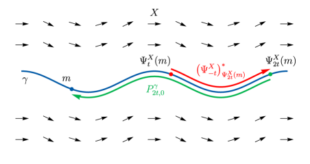
Figure 1. $\nabla^{s}$-parallel transport.

Remark 2.19.

The interpretation in terms of the $\nabla^{s}$-parallel transport of Proposition 2.18 makes it possible to define the symmetric Lie derivative for arbitrary tensor fields. Formula (10) is then satisfied in general.

2.6. The symmetric bracket

By analogy with the formula $\iota_{[X,Y]}=[L_{X},\iota_{Y}]_{g}$, the corresponding bracket $\langle\,\,:\,\,\rangle_{s}$ in the symmetric setting should be determined by

(14) $$\iota_{\langle X:Y\rangle_{s}}=[L^{s}_{X},\iota_{Y}]=L_{X}^{s}\circ\iota_{Y}-\iota_{Y}\circ L_{X}^{s}.$$

Since the right-hand side is a derivation of degree $(-1)$ and, by Lemma 2.1, any such derivation is the interior multiplication by a unique vector field, equation (14) determines uniquely the symmetric bracket $\langle\,\,:\,\,\rangle_{s}$. We can find an explicit expression as, for $\alpha\in\Upsilon^{1}(M)$,

$$L^{s}_{X}\iota_{Y}\alpha-\iota_{Y}L_{X}^{s}\alpha =X\alpha(Y)-(\nabla_{X}\alpha)(Y)+\alpha(\nabla_{Y}X)$$

$$=\alpha(\nabla_{X}Y+\nabla_{Y}X)=\iota_{(\nabla_{X}Y+\nabla_{Y}X)}\alpha.$$

Definition 2.20.

The symmetric bracket corresponding to a connection $\nabla$ on $M$ is given, for $X,Y\in\mathfrak{X}(M)$, by

(15) $$\langle X:Y\rangle_{s}=\nabla_{X}Y+\nabla_{Y}X.$$

Example 2.21.

Let $g$ be a (pseudo-)Riemannian metric. We have the following formula for the symmetric bracket corresponding to the Levi-Civita connection $\prescript{g}{}{\nabla}$:

(16) $$\langle X:Y\rangle_{s}=g^{-1}(L_{X}g(Y)+L_{Y}g(X))-\operatorname{grad}_{g}g(X,Y),$$

where $\operatorname{grad}_{g}:\mathcal{C}^{\infty}(M)\rightarrow\mathfrak{X}(M)$ is the natural map given by $\operatorname{grad}_{g}:=g^{-1}\circ\mathrm{d}$.

Remark 2.22.

Formula (16) can be reinterpreted, by using $\vartheta:=g^{-1}$, as a symmetric bracket on the cotangent bundle: for $\alpha,\beta\in\Omega^{1}(M)$,

(17) $$\langle\alpha:\beta\rangle_{\vartheta}:=L_{\vartheta(\alpha)}\beta+L_{\vartheta(\beta)}\alpha-\mathrm{d}\vartheta(\alpha,\beta).$$

The bracket in (17) can be defined for an arbitrary $\vartheta\in\mathfrak{X}^{2}_{\text{sym}}(M)$, possibly degenerate. It turns out to be a symmetric analogue of the Lie algebroid bracket on the cotangent bundle of a Poisson manifold $(M,\pi)$ (see, for instance, [8]):

$$[\alpha,\beta]_{\pi}:=L_{\pi(\alpha)}\beta-L_{\pi(\beta)}\alpha-\mathrm{d}\pi(\alpha,\beta).$$

Analogues of the usual identities for the Lie bracket, the exterior and Lie derivatives also hold here. On the one hand,

(18) $$L_{X}^{s}Y=\langle X:Y\rangle_{s}=L_{Y}^{s}X,$$

which follows by applying $L_{X}Y=\nabla^{0}_{X}Y-\nabla^{0}_{Y}X$ and (10). On the other hand, from (7) and (9), we have, for $\varphi\in\Upsilon^{r}(M)$ and $X,X_{j}\in\mathfrak{X}(M)$,

$$(\nabla^{s}\varphi)(X_{1},\makebox[10.00002pt][c]{.\hfil.\hfil.},X_{r+1})=\, \sum_{j=1}^{r+1}X_{j}\,\varphi(X_{1},\makebox[10.00002pt][c]{.\hfil.\hfil.},\hat{X}_{j},\makebox[10.00002pt][c]{.\hfil.\hfil.},X_{r+1})$$

$$-\sum_{\underset{i<j}{i,j=1,}}^{r+1}\varphi(\langle X_{i}:X_{j}\rangle_{s},X_{1},\makebox[10.00002pt][c]{.\hfil.\hfil.},\hat{X}_{i},\makebox[10.00002pt][c]{.\hfil.\hfil.},\hat{X}_{j},\makebox[10.00002pt][c]{.\hfil.\hfil.},X_{r+1}),$$

$$(L^{s}_{X}\varphi)(X_{1},\makebox[10.00002pt][c]{.\hfil.\hfil.},X_{r})= \,X\,\varphi(X_{1},\makebox[10.00002pt][c]{.\hfil.\hfil.},X_{k})-\sum_{j=1}^{r}\varphi(\langle X:X_{j}\rangle_{s},X_{1},\makebox[10.00002pt][c]{.\hfil.\hfil.},\hat{X}_{j},\makebox[10.00002pt][c]{.\hfil.\hfil.},X_{r}).$$

2.7. Geometric interpretation of the symmetric bracket

As a consequence of (18) and Proposition 2.18, the symmetric bracket measures the invariance of a vector field with respect to the $\nabla^{s}$-parallel transport. A different interpretation, in terms of a second derivative of commutator of flows, is given in [2, Sec. 3].

We recall now an additional geometric interpretation of the symmetric bracket [17], which describes the properties of involutive distributions.

For a connection $\nabla$ on $M$, a smooth distribution $\Delta\subseteq TM$ is $\nabla$-geodesically invariant if each $\nabla$-geodesic $\gamma:I\rightarrow M$ defined on some open interval $I\subseteq\mathbb{R}$ possesses the property that existence of $t_{0}\in I$ such that $\dot{\gamma}(t_{0})\in\Delta_{\gamma(t_{0})}$ implies that $\dot{\gamma}(t)\in\Delta_{\gamma(t)}$ for all $t\in I$. A submanifold $S\subseteq M$ is called totally $\nabla$-geodesic if every $\nabla$-geodesic on $M$ that intersects $S$ is completely contained in $S$.

Remark 2.23.

Note that if a geodesically invariant distribution is, in addition, integrable, it corresponds to a foliation by totally geodesic submanifolds.

The geometric interpretation for the symmetric bracket is analogous to Frobenius theorem for integrable distributions.

Theorem 2.24 ([17]).

For a connection $\nabla$ on $M$, a smooth distribution $\Delta\subseteq TM$ with locally constant rank is $\nabla$-geodesically invariant if and only if

$$\langle\Gamma(\Delta):\Gamma(\Delta)\rangle_{s}\subseteq\Gamma(\Delta).$$

In [5], the role of the bracket in theoretical mechanics is discussed.

3. Commutation relations of symmetric Cartan calculus

The classical Cartan calculus on differential forms $\Omega^{\bullet}(M)$ is characterized by the graded-commutation relations between $\iota$, $\mathrm{d}$ and $L$:

$$[\iota_{X},\iota_{Y}]_{\text{g}} =0, [\mathrm{d},\mathrm{d}]_{\text{g}} =0, [\iota_{X},\mathrm{d}]_{\text{g}} =L_{X},$$

$$[L_{X},\iota_{Y}]_{\text{g}} =\iota_{[X,Y]}, [L_{X},L_{Y}]_{\text{g}} =L_{[X,Y]}, [\mathrm{d},L_{X}]_{\text{g}} =0.$$

Just as graded derivations are closed under the graded commutator, derivations are closed under the commutator. Thus, for the symmetric Cartan calculus on $\Upsilon^{\bullet}(M)$, we aim to have similar relations between $\iota$, $\nabla^{s}$ and $L^{s}$ and the usual commutator.

As $\Upsilon^{\bullet}(M)$ is the space of symmetric forms on $M$ we have

$$[\iota_{X},\iota_{Y}]=0.$$

The analogue of the second relation

$$[\nabla^{s},\nabla^{s}]=0$$

is also satisfied trivially because of the skew-symmetry of the commutator. The analogues of the third and fourth formulas were used to define the symmetric Lie derivative (Definition 2.14) and derive the symmetric bracket (14), that is,

$$[\iota_{X},\nabla^{s}]=L^{s}_{X}, [L^{s}_{X},\iota_{Y}]=\iota_{\langle X:Y\rangle_{s}}.$$

For the remaining two identities, we will find that the analogues are more involved. In the case of $[L_{X},L_{Y}]_{\text{g}}=L_{[X,Y]}$, it is clear that $[L^{s}_{X},L^{s}_{Y}]\neq L^{s}_{\langle X:Y\rangle_{s}}$ since the left-hand side is skew-symmetric on $X$ and $Y$, whereas the right-hand side is symmetric. Their proof will require the extension of the contraction operator and the symmetric derivative (Sections 3.1 and 3.3).

3.1. The symmetric contraction operator

Since this is a linear-algebraic operator, we first work on a vector space $V$ and then globalize it. Consider $\sigma\in\operatorname{Sym}^{k}V^{*}\otimes V$. The symmetric contraction operator

$$\iota^{s}_{\sigma}:\operatorname{Sym}^{\bullet}V^{*}\rightarrow\operatorname{Sym}^{\bullet}V^{*}$$

is the unique degree-$(k-1)$ derivation of $\operatorname{Sym}^{\bullet}V^{*}$ determined by its action on $\lambda\in{\mathbb{R}}$ and $\alpha\in V^{*}$ by

$$\iota^{s}_{\sigma}\lambda:=0, \iota^{s}_{\sigma}\alpha:=\iota_{\sigma}\alpha,$$

where by $\iota_{\sigma}$ we mean, for $\varphi\in\operatorname{Sym}^{r}V^{*}$,

$$(\iota_{\sigma}\varphi)(X_{1},\makebox[10.00002pt][c]{.\hfil.\hfil.},X_{r+k-1}):=\varphi(\sigma(X_{1},\makebox[10.00002pt][c]{.\hfil.\hfil.},X_{k}),X_{k+1},\makebox[10.00002pt][c]{.\hfil.\hfil.},X_{r+k-1}).$$

We easily see that a generalization of Lemma 2.1 is true. Namely, the map $\iota^{s}:\sigma\mapsto\iota^{s}_{\sigma}$ gives an isomorphism of graded vector spaces:

$$\operatorname{Sym}^{\bullet}V^{*}\otimes V\overset{\sim}{\longleftrightarrow}\left\{\begin{array}[]{c}\text{derivations of $\operatorname{Sym}^{\bullet}V^{*}$ that}\\ \text{annihilate scalars $\operatorname{Sym}^{0}V^{*}={\mathbb{R}}$}\end{array}\right\}.$$

Lemma 3.1.

Let $\varphi\in\operatorname{Sym}^{r}V^{*}$ and $\sigma\in\operatorname{Sym}^{k}V^{*}\otimes V$. The symmetric contraction operator is explicitly given by

$$\iota^{s}_{\sigma}\varphi=\frac{(r+k-1)!}{(r-1)!k!}\operatorname{sym}\iota_{\sigma}\varphi.$$

Proof.

The endomorphism on the right-hand side is clearly a degree-$(k-1)$ map and coincides with $\iota^{s}_{\sigma}$ on scalars and $1$-forms. Therefore, it is enough to check that it is a derivation of $\operatorname{Sym}^{\bullet}V^{*}$, which is done analogously to Lemma 2.1. ∎

Globally, the symmetric contraction operator by an element of $\Upsilon^{k}(M,TM)$ (in the sense of Remark 2.3) becomes an element of $\mathrm{Der}_{k-1}(\Upsilon^{\bullet}(M))$.

3.2. Commutator of symmetric Lie derivatives

We can now deal with the analogue of the fifth identity.

Proposition 3.2.

Let $\nabla$ be a torsion-free connection on $M$. For $X,Y\in\mathfrak{X}(M)$,

(19) $$[L^{s}_{X},L^{s}_{Y}]=L^{s}_{[X,Y]}+\iota^{s}_{2(\nabla_{\nabla X}Y-\nabla_{\nabla Y}X-R_{\nabla}(X,Y))},$$

where $R_{\nabla}$ is the Riemann curvature tensor.

Proof.

As all the terms are derivations of $\Upsilon^{\bullet}(M)$, it is enough to check the equality on functions and $1$-forms. Functions are annihilated by any symmetric contraction operator, so the relation is clearly satisfied as $L^{s}_{X}f=Xf$. For an arbitrary $1$-form $\alpha\in\Upsilon^{1}(M)$ we have

$$([L^{s}_{X},L^{s}_{Y} ]\alpha)(Z)-(L^{s}_{[X,Y]}\alpha)(Z)$$

$$=\, X(L^{s}_{Y}\alpha)(Z)-(L^{s}_{Y}\alpha)(\langle X:Z\rangle_{s})-Y(L^{s}_{X}\alpha)(Z)+(L^{s}_{X}\alpha)(\langle Y:Z\rangle_{s})$$

$$-[X,Y]\alpha(Z)+\alpha(\langle[X,Y]:Z\rangle_{s})$$

$$=\, X(Y\alpha(Z))-X\alpha(\langle Y:Z\rangle_{s})-Y\alpha(\langle X:Z\rangle_{s})+\alpha(\langle Y:\langle X:Z\rangle_{s}\rangle_{s})$$

$$-Y(X\alpha(Z))+Y\alpha(\langle X:Z\rangle_{s})+X\alpha(\langle Y:Z\rangle_{s})-\alpha(\langle X:\langle Y:Z\rangle_{s}\rangle_{s})$$

$$-[X,Y]\alpha(Z)+\alpha(\langle[X,Y]:Z\rangle_{s})$$

$$=\, \alpha(W),$$

where $W\in\mathfrak{X}(M)$ is given by $W:=\langle\langle X:Z\rangle_{s}:Y\rangle_{s}-\langle X:\langle Y:Z\rangle_{s}\rangle_{s}+\langle[X,Y]:Z\rangle_{s}$. Explicitly,

$$W= \nabla_{Y}\nabla_{X}Z+\nabla_{Y}\nabla_{Z}X+\nabla_{\nabla_{X}Z+\nabla_{Z}X}Y-\nabla_{X}\nabla_{Y}Z$$

$$-\nabla_{X}\nabla_{Z}Y-\nabla_{\nabla_{Y}Z+\nabla_{Z}Y}X+\nabla_{[X,Y]}Z+\nabla_{Z}[X,Y].$$

Using the definition of the curvature tensor and the torsion-freeness of $\nabla$, we get

$$W=-R_{\nabla}(X,Y)Z+R_{\nabla}(Y,Z)X+R_{\nabla}(Z,X)Y+2(\nabla_{\nabla_{Z}X}Y-\nabla_{\nabla_{Z}Y}X).$$

Finally, it follows from the algebraic Bianchi identity that

$$([L^{s}_{X},L^{s}_{Y}]\alpha)(Z)-(L^{s}_{[X,Y]}\alpha)(Z)=\alpha(2(\nabla_{\nabla_{Z}X}Y-\nabla_{\nabla_{Z}Y}X-R_{\nabla}(X,Y)Z)).$$

∎

3.3. Extension of the symmetric derivative and the symmetric curvature

Similarly as we generalized the contraction operator, we generalize also the symmetric derivative.

Definition 3.3.

Let $\nabla$ be a connection on $M$ and $A\in\Gamma(\operatorname{\mathrm{End}}TM)$. We introduce the $A$-symmetric derivative of $\nabla^{s}_{A}\in\mathrm{Der}_{1}(\Upsilon^{\bullet}(M))$ by the formula

$$\nabla^{s}_{A}:=[\iota^{s}_{A},\nabla^{s}].$$

Remark 3.4.

Note that $\iota^{s}_{\operatorname{id}}\varphi=r\,\varphi$ for every $\varphi\in\Upsilon^{r}(M)$. Therefore, $\nabla^{s}=\nabla^{s}_{\operatorname{id}_{TM}}$.

The last piece to be introduced is a symmetric analogue of the curvature operator, whose definition will rely on the concept of second covariant derivative. This is, for a connection $\nabla$ on $M$, the linear map $\nabla^{2}:\mathfrak{X}(M)\rightarrow\Gamma(\otimes^{2}T^{*}M\otimes TM)$ defined by

$$(\nabla^{2}X)(Y,Z):=(\nabla\nabla X)(Y,Z)=\nabla_{Y}\nabla_{Z}X-\nabla_{\nabla_{Y}Z}X.$$

Note that the map is not $\mathcal{C}^{\infty}(M)$-linear. However, when we take its skew-symmetric part and the connection is torsion-free, it is and we recover the Riemann curvature tensor $R_{\nabla}\in\Omega^{2}(M,\operatorname{\mathrm{End}}TM)$:

$$(2\operatorname{skew}\nabla^{2}X)(Y,Z)=\nabla_{Y}\nabla_{Z}X-\nabla_{Z}\nabla_{Y}X-\nabla_{[Y,Z]}X=R_{\nabla}(Y,Z)X.$$

Definition 3.5.

Let $\nabla$ be a connection on $M$. We introduce the symmetric curvature operator $R^{s}_{\nabla}:\mathfrak{X}(M)\rightarrow\Upsilon^{2}(M,TM)$ by the formula

$$(R^{s}_{\nabla}X)(Y,Z):=(2\operatorname{sym}\nabla^{2}X)(Y,Z)=\nabla_{Y}\nabla_{Z}X+\nabla_{Z}\nabla_{Y}X-\nabla_{\langle Y:Z\rangle_{s}}X.$$

Remark 3.6.

If $\nabla$ is a torsion-free connection on $M$, we can express the second covariant derivative in terms of the corresponding Riemannian curvature tensor and symmetric curvatures operator:

$$(\nabla^{2}X)(Y,Z)=\frac{1}{2}(R_{\nabla}(Y,Z)X+(R^{s}_{\nabla}X)(Y,Z)).$$

A geometric interpretation of the symmetric curvature operator will be given in Remark 4.15.

3.4. Commutator of symmetric and symmetric Lie derivatives

We prove now the remaining identity of symmetric Cartan calculus.

Proposition 3.7.

Let $\nabla$ be a torsion-free connection. For $X\in\mathfrak{X}(M)$,

(20) $$[\nabla^{s},L^{s}_{X}]=2\nabla^{s}_{\nabla X}+\iota^{s}_{2\operatorname{sym}\iota_{X}R_{\nabla}+R^{s}_{\nabla}X}.$$

Proof.

Analogously as in Proposition 3.2, it is enough to check the relation on $\mathcal{C}^{\infty}(M)$ and $\Upsilon^{1}(M)$. The relation (20) restricted on functions says

$$2\mathrm{d}\circ\iota_{X}\circ\mathrm{d}-\iota_{X}\circ\nabla^{s}\circ\mathrm{d}=2\iota_{\nabla X}\circ\mathrm{d}.$$

The left-hand side acting on $f\in\mathcal{C}^{\infty}(M)$ and evaluated on $Y\in\mathfrak{X}(M)$ gives

$$2Y(Xf)-(\nabla^{s}\mathrm{d}f)(X,Y) =Y(Xf)-X(Yf)+\langle X:Y\rangle_{s}f$$

$$=([X,Y]+\langle X:Y\rangle_{s})f=2(\nabla_{Y}X)f=2(\iota_{\nabla X}\mathrm{d}f)(Y),$$

where the second equality follows from torsion-freeness of $\nabla$. For $\alpha\in\Upsilon^{1}(M)$,

$$([\nabla^{s} ,L^{s}_{X}]\alpha)(Y,Y)-2(\nabla^{s}_{\nabla X}\alpha)(Y,Y)$$

$$=\, (\nabla^{s}L^{s}_{X}\alpha)(Y,Y)-(L^{s}_{X}\nabla^{s}\alpha)(Y,Y)-2(\iota^{s}_{\nabla X}\nabla^{s}\alpha)(Y,Y)+2(\nabla^{s}\iota_{\nabla X}\alpha)(Y,Y)$$

$$=\, 2Y(L^{s}_{X}\alpha)(Y)-(L^{s}_{X}\alpha)(\langle Y:Y\rangle_{s})-X(\nabla^{s}\alpha)(Y,Y)+2(\nabla^{s}\alpha)(\langle X:Y\rangle_{s},Y)$$

$$-4(\nabla^{s}\alpha)(\nabla_{Y}X,Y)+4Y\alpha(\nabla_{Y}X)-2\alpha(\nabla_{\langle Y:Y\rangle_{s}}X)$$

$$=\, 2Y(X\alpha(Y))-2Y\alpha(\langle X:Y\rangle_{s})-X\alpha(\langle Y:Y\rangle_{s})+\alpha(\langle X:\langle Y:Y\rangle_{s}\rangle)$$

$$-2X(Y\alpha(Y))+X\alpha(\langle Y:Y\rangle_{s})+2\langle X:Y\rangle_{s}\alpha(Y)+2Y\alpha(\langle X:Y\rangle_{s})$$

$$-2\alpha(\langle\langle X:Y\rangle_{s}:Y\rangle_{s})-4(\nabla_{Y}X)\alpha(Y)-4Y\alpha(\nabla_{Y}X)+4\alpha(\langle\nabla_{Y}X:Y\rangle_{s})$$

$$+4Y\alpha(\nabla_{Y}X)-2\alpha(\nabla_{\langle Y:Y\rangle_{s}}X).$$

Using the fact that $\nabla$ is torsion-free we get

$$([\nabla^{s},L^{s}_{X}]\alpha)(Y,Y)-2(\nabla^{s}_{\nabla X}\alpha)(Y,Y)=\alpha(W),$$

where $W\in\mathfrak{X}(M)$ is given by

$$W =\langle X:\langle Y:Y\rangle_{s}\rangle_{s}-2\langle\langle X:Y\rangle_{s},Y\rangle_{s}+4\langle\nabla_{Y}X:Y\rangle_{s}-2\nabla_{\langle Y:Y\rangle_{s}}X)$$

$$=2\nabla_{X}\nabla_{Y}Y+2\nabla_{\nabla_{Y}Y}X-2\nabla_{\nabla_{X}Y+\nabla_{Y}X}Y-2\nabla_{Y}\nabla_{X}Y$$

$$\phantom{=}-2\nabla_{Y}\nabla_{Y}X+4\nabla_{\nabla_{Y}X}Y+4\nabla_{Y}\nabla_{Y}X-4\nabla_{\nabla_{Y}Y}X.$$

It follows from the torsion-freeness of $\nabla$ that $W$ may be rewritten in terms of the Riemann curvature tensor and the symmetric curvature operator:

$$W=2R_{\nabla}(X,Y)Y+(R^{s}_{\nabla}X)(Y,Y)=(2\operatorname{sym}\iota_{X}R_{\nabla}+R^{s}_{\nabla}X)(Y,Y).$$

Finally, it follows from the polarization identity that

$$([\nabla^{s},L^{s}_{X}]\alpha)(Y,Z)-2(\nabla^{s}_{\nabla X}\alpha)(Y,Z)=\alpha((2\operatorname{sym}\iota_{X}R_{\nabla}+R^{s}_{\nabla}X)(Y,Z)).$$

∎

Identities (19) and (20) involve rather complicated terms. We will be able to say more about them in Section 5.4, once we have described affine morphisms in Section 4.

3.5. Dependence on the connection

The symmetric contraction operator introduced in Section 3.1 allows us to describe how the symmetric Cartan calculus varies when we change the connection.

Proposition 3.8.

Let $\nabla$ and $\nabla^{\prime}$ be two torsion-free connections on $M$, then

$$\nabla^{\prime}_{X}Y=\nabla_{X}Y-\frac{1}{2}\sigma(X,Y)$$

for a unique $\sigma\in\Upsilon^{2}(M,TM)$. The corresponding symmetric derivatives, symmetric Lie derivatives and symmetric brackets are related as follows:

$$\nabla^{\prime s}=\nabla^{s}+\iota^{s}_{\sigma}, L^{\prime s}_{X}=L^{s}_{X}+\iota^{s}_{\sigma(X,\,\,)}, \langle X:Y\rangle^{\prime}_{s}=\langle X:Y\rangle_{s}-\sigma(X,Y).$$

Proof.

The statement for symmetric brackets is trivial. It is enough to check the other two relations on functions and $1$-forms. The equalities on functions follow from that every symmetric contraction operator annihilate functions, every symmetric derivative is geometric and $L^{s}_{X}f=Xf=L^{\prime s}_{X}f$. The equalities on $1$-forms follow by straightforward calculations provided the relation between symmetric brackets. ∎

4. Affine manifold morphisms

We study now affine morphisms, which are the natural transformations in presence of a connection. We will see how they interact with symmetric Cartan calculus and also their infinitesimal version. Some of the results of this section are stated for arbitrary connections since they provide stronger versions.

4.1. Definition of affine morphisms

Given two manifolds $M$ and $M^{\prime}$, any diffeomorphism $\phi:M\rightarrow M^{\prime}$ intertwines their Cartan calculi in the sense that,

$$\phi_{*}[X,Y] =[\phi_{*}X,\phi_{*}Y], \phi^{*}\circ\mathrm{d} =\mathrm{d}\circ\phi^{*}, \phi^{*}\circ L_{\phi_{*}X} =L_{X}\circ\phi^{*}.$$

For symmetric Cartan calculus, the notion of affine diffeomorphism will play an analogous role. In this section, connections are not necessarily torsion-free.

Definition 4.1.

Given two manifolds with connection $(M,\nabla)$ and $(M^{\prime},\nabla^{\prime})$, a smooth map $\phi:M\rightarrow M^{\prime}$ is an affine morphism if $\phi_{*}$ commutes with the corresponding parallel transports $P$ and $P^{\prime}$, that is,

$$\phi_{*\gamma(t_{1})}\circ P^{\gamma}_{t_{0},t_{1}}=P^{\prime\phi\circ\gamma}_{t_{0},t_{1}}\circ\phi_{*\gamma(t_{0})},$$

for any curve $\gamma:I\rightarrow M$ and $t_{0},t_{1}\in I$. If, in addition, $\phi$ is a diffeomorphism, we call it affine diffeomorphism. We denote the space of affine diffeomorphisms by $\mathrm{Aff}(\nabla,\nabla^{\prime})$, and $\mathrm{Aff}(\nabla)$ if $M=M^{\prime}$ and $\nabla=\nabla^{\prime}$.

It is well known that the group of isometries of a (pseudo-)Riemannian metric is a Lie group of dimension at most $\frac{1}{2}n(n+1)$, where $n:=\dim M$. A similar result is true also for the group $\mathrm{Aff}(\nabla)$.

Theorem 4.2 ([15]).

Let $\nabla$ be a connection on $M$ of dimension $n\in\mathbb{N}$. The group $\mathrm{Aff}(\nabla)$ is a Lie group of dimension at most $n(n+1)$.

Example 4.3.

In the simplest case, the Euclidean connection $\nabla^{\text{Euc}}$ on $\mathbb{R}^{n}$, we have $\mathrm{Aff}(\nabla^{\text{Euc}})\cong\mathrm{Aff}(n,{\mathbb{R}}):=\mathrm{GL}(n,{\mathbb{R}})\ltimes{\mathbb{R}}^{n}$, thus attaining the maximal dimension.

Example 4.4.

Every isometry between two (pseudo-)Riemannian metrics is an affine diffeomorphism between the corresponding Levi-Civita connections, see e.g. [15]. However, the converse is not true in general as it is clear from Example 4.3.

A simpler characterization of affine morphisms will prove useful.

Proposition 4.5.

A map $\phi:M\rightarrow M^{\prime}$ is an affine morphism if and only if

$$\nabla\circ\phi^{*}=\phi^{*}\circ\nabla^{\prime},$$

where $\nabla$ is seen as a map $\Omega^{1}(M)\rightarrow\Omega^{1}(M,T^{*}M)$.

Proof.

Recall that if $P^{\gamma}_{t_{0},t_{1}}$ is the $\nabla$-parallel transport from $t_{0}$ to $t_{1}$ along $\gamma$, its algebraic transpose is the parallel transport from $t_{1}$ to $t_{0}$ along $\gamma$ for the dual connection on $T^{*}M$, which we denote by ${P^{*}}^{\gamma}_{t_{1},t_{0}}$. Therefore, a map $\phi:M\rightarrow M^{\prime}$ is an affine morphism if and only if

(21) $${P^{*}}^{\gamma}_{t_{0},t_{1}}\circ\phi^{*}_{\gamma(t_{0})}=\phi^{*}_{\gamma(t_{1})}\circ{P^{\prime*}}^{\phi\circ\gamma}_{t_{0},t_{1}}.$$

Consider an arbitrary vector vector $X\in T_{m}M$ and $\alpha\in\Omega^{1}(M^{\prime})$. We have,

$$(\nabla_{X}\phi^{*}\alpha)_{m}=\lim_{t\to 0}\frac{1}{t}({P^{*}}^{\gamma}_{t,0}\phi^{*}_{\gamma(t)}\alpha_{\phi(\gamma(t))}-\phi^{*}_{m}\alpha_{\phi(m)}),$$

where $\gamma:I\rightarrow M$ is an arbitrary curve such that $\dot{\gamma}(0)=X$. Assume first that $\phi$ is an affine morphism. It follows from (21) that

$$(\nabla_{X}\phi^{*}\alpha)_{m} =\lim_{t\to 0}\frac{1}{t}(\phi^{*}_{m}{P^{\prime*}}^{\phi\circ\gamma}_{t,0}\alpha_{\phi(\gamma(t))}-\phi^{*}_{m}\alpha_{\phi(m)})=\phi^{*}_{m}\lim_{t\to 0}\frac{1}{t}({P^{\prime*}}^{\phi\circ\gamma}_{t,0}\alpha_{\phi(\gamma(t))}-\alpha_{\phi(m)})$$

$$=\phi^{*}_{m}(\nabla^{\prime}_{\phi_{*m}X}\alpha)_{\phi(m)}.$$

Conversely, assume that $\nabla\circ\phi^{*}=\phi^{*}\circ\nabla^{\prime}$ is true. Consider an arbitrary curve $\gamma:I\rightarrow M$, $t_{0},t_{1}\in I$ and $\zeta\in T^{*}_{\phi(\gamma(t_{0}))}M^{\prime}$. To prove that $\phi$ is an affine morphism, by (21), it is enough to show that the $1$-form $\alpha\in\Gamma(\gamma^{*}TM)$ defined, for $t\in I$, by

$$\alpha(t) :=\phi^{*}_{\gamma(t)}\beta(t), \beta(t) :={P^{\prime*}}^{\phi\circ\gamma}_{t_{0},t}\zeta,$$

satisfies $\nabla_{\dot{\gamma}}\alpha=0$. This follows from $\nabla^{\prime}_{\phi_{*}\dot{\gamma}}\beta=0$, as

$$\nabla_{\dot{\gamma}}\alpha=\nabla_{\dot{\gamma}}\phi^{*}\beta=\phi^{*}\nabla^{\prime}_{\phi_{*}\dot{\gamma}}\beta=0.$$

∎

For affine diffeomorphisms, we can reformulate Proposition 4.5 in terms of the original connection on $TM$.

Proposition 4.6 (e.g., [16]).

A diffeomorphism $\phi:M\rightarrow M^{\prime}$ is an affine diffeomorphism if and only if, for all $X,Y\in\mathfrak{X}(M)$,

$$\phi_{*}(\nabla_{X}Y)=\nabla^{\prime}_{\phi_{*}X}\phi_{*}Y$$

Given a diffeomorphism $\phi:M\rightarrow M^{\prime}$ and a connection $\nabla^{\prime}$ on $M^{\prime}$, the pullback connection $\phi^{*}\nabla^{\prime}$ on $M$ is given for $X,Y\in\mathfrak{X}(M)$ by

$$(\phi^{*}\nabla^{\prime})_{X}Y:=\phi^{-1}_{*}\nabla^{\prime}_{\phi_{*}X}\phi_{*}Y.$$

Corollary 4.7.

Let $\phi:M\rightarrow M^{\prime}$ be a diffeomorphism and $\nabla^{\prime}$ be a connection on $M^{\prime}$. Then $\phi\in\mathrm{Aff}(\phi^{*}\nabla^{\prime},\nabla^{\prime})$.

Remark 4.8.

Since $\phi_{*}$ preserves the Lie bracket of vector fields, we get

$$T_{\phi^{*}\nabla^{\prime}}(X,Y)=\phi^{-1}_{*}T_{\nabla^{\prime}}(\phi_{*}X,\phi_{*}Y).$$

Therefore, $\phi^{*}\nabla^{\prime}$ is torsion-free if and only if $\nabla^{\prime}$ is torsion-free.

4.2. Relation to symmetric Cartan calculus

In case of torsion-free connections, we can rephrase Proposition 4.5 using the symmetric derivatives.

Corollary 4.9.

Let $\nabla$ and $\nabla^{\prime}$ be torsion-free connections on $M$ and $M^{\prime}$ respectively. A smooth map $\phi:M\rightarrow M^{\prime}$ is an affine morphism if and only if

$$\nabla^{s}\circ\phi^{*}=\phi^{*}\circ{\nabla^{\prime}}^{s}.$$

Remark 4.10.

Note that if $\nabla$ and $\nabla^{\prime}$ are not torsion-free, we can only claim that if $\phi:M\rightarrow M^{\prime}$ is an affine morphism, then $\nabla^{s}\circ\phi^{*}=\phi^{*}\circ\nabla^{\prime s}$.

The relation between affine diffeomorphisms and symmetric Cartan calculus is described by the following result.

Proposition 4.11.

Let $\nabla$ and $\nabla^{\prime}$ be connections on $M$ and $M^{\prime}$ and denote the associated torsion-free connections by $\nabla^{0}$ and $\nabla^{\prime 0}$ respectively. Then the following statements about a diffeomorphism $\phi:M\rightarrow M^{\prime}$ are equivalent:

1. $\phi\in\mathrm{Aff}(\nabla^{0},\nabla^{\prime 0})$;

2. $\phi^{*}\circ\nabla^{\prime s}=\nabla^{s}\circ\phi^{*}$;

3. $\phi^{*}\circ L^{s}_{\phi_{*}X}=L^{s}_{X}\circ\phi^{*}$ for all $X\in\mathfrak{X}(M)$;

4. $\phi_{*}\langle X:Y\rangle_{s}=\langle\phi_{*}X:\phi_{*}Y\rangle_{s}$ for all $X,Y\in\mathfrak{X}(M)$.

Proof.

The equivalence between (1) and (2) is given by Corollary 4.9. We see that (2) implies (3) by using the identity $\iota_{X}\circ\phi^{*}=\phi^{*}\circ\iota_{\phi_{*}X}$:

$$\phi^{*}\circ L^{s}_{\phi_{*}X} =\phi^{*}\circ\iota_{\phi_{*}X}\circ\nabla^{s}-\phi^{*}\circ\nabla^{s}\circ\iota_{\phi_{*}X}$$

$$=\iota_{X}\circ\nabla^{s}\circ\phi^{*}-\nabla^{s}\circ\iota_{X}\circ\phi^{*}$$

$$=L_{X}^{s}\circ\phi^{*}.$$

To see that (3) implies (4), simply consider (3) for any $\alpha\in\Upsilon^{1}(M^{\prime})$, $X,Y\in\mathfrak{X}(M)$, and $m\in M$, that is,

$$0=\, ((\phi^{*}L^{s}_{\phi_{*}X}\alpha)(Y))(m)-((L^{s}_{X}\phi^{*}\alpha)(Y))(m)$$

$$=\, ((L_{\phi_{*}X}^{s}\alpha)(\phi_{*}Y))(\phi(m))-((L^{s}_{X}\phi^{*}\alpha)(Y))(m)$$

$$=\, ((\phi_{*}X)\alpha(\phi_{*}Y))(\phi(m))-\alpha_{\phi(m)}(\left.\langle\phi_{*}X:\phi_{*}Y\rangle_{s}\right|_{\phi(m)})$$

$$-(X(\phi^{*}\alpha)(Y))(m)+(\phi^{*}\alpha)_{m}(\left.\langle X:Y\rangle_{s}\right|_{m})$$

$$=\, \alpha_{\phi(m)}(\left.\langle\phi_{*}X:\phi_{*}Y\rangle_{s}\right|_{\phi(m)}-\left.(\phi_{*}\langle X:Y\rangle_{s})\right|_{\phi(m)}).$$

Finally, the equivalence between (4) and (1) follows from Proposition 4.6 and the identities

$$\phi_{*}\nabla^{0}_{X}Y =\frac{1}{2}(\phi_{*}\langle X:Y\rangle_{s}+\phi_{*}[X,Y]),$$

$$\nabla^{0}_{\phi_{*}X}\phi_{*}Y =\frac{1}{2}(\langle\phi_{*}X:\phi_{*}Y\rangle_{s}+[\phi_{*}X,\phi_{*}Y]).$$

∎

4.3. Affine vector fields

The infinitesimal version of an affine diffeomorphism from the manifold to itself is a vector field whose flow is a local $1$-parameter subgroup of affine diffeomorphisms. We call such vector field an affine vector field. There is a useful equivalent characterization of affine vector fields.

Proposition 4.12 ([15]).

Let $\nabla$ be a connection on $M$. A vector field $X\in\mathfrak{X}(M)$ is affine if and only if, for all $Y,Z\in\mathfrak{X}(M)$,

(22) $$[L_{X},\nabla_{Y}]Z=\nabla_{[X,Y]}Z.$$

Example 4.13.

Consider a (pseudo-)Riemannian manifold $(M,g)$. A Killing vector field of $g$ is a vector field on $M$ whose flow is a local $1$-parameter subgroup of isometries. Equivalently, $X\in\mathfrak{X}(M)$ is a Killing vector field if $L_{X}g=0$. In particular, every Killing vector field is an affine vector field for the corresponding Levi-Civita connection. However, the converse is not true in general. For instance, the vector field $X:=x^{i}\partial_{x^{i}}\in\mathfrak{X}({\mathbb{R}}^{n})$ is not a Killing vector field for the Euclidean metric $g^{\text{Euc}}$ as

$$L_{X}g^{\text{Euc}}=2g^{\text{Euc}}\neq 0,$$

but it is an affine vector field for the Euclidean connection.

If the connection is torsion-free, there are three more equivalent formulae characterizing affine vector fields that are closely related to symmetric Cartan calculus and will also be relevant in Section 5.4.

Proposition 4.14.

Let $\nabla$ be a torsion-free connection on $M$. A vector field $X\in\mathfrak{X}(M)$ is an affine vector field if and only if one of the following equivalent statements is true

1. $2\operatorname{sym}\iota_{X}R_{\nabla}+R^{s}_{\nabla}X=0$,

2. $[X:\langle Y:Z\rangle_{s}]=\langle[X,Y]:Z\rangle_{s}+\langle Y:[X,Z]\rangle_{s}$ for all $Y,Z\in\mathfrak{X}(M)$.

3. $[\nabla^{s},L_{X}]=0$.

Proof.

Using the fact that $\nabla$ is torsion-free, we can rewrite the relation (22) as

$$\nabla_{X}\nabla_{Y}Z-\nabla_{\nabla_{Y}Z}X-\nabla_{Y}\nabla_{X}Z+\nabla_{Y}\nabla_{Z}X=\nabla_{[X,Y]}Z.$$

Taking all the terms on the left-hand side yields $R_{\nabla}(X,Y)Z+(\nabla^{2}X)(Y,Z)=0$. This is thanks to Remark 3.6 equivalent to

$$2R_{\nabla}(X,Y)Z+R_{\nabla}(Y,Z)X+(R^{s}_{\nabla}X)(Y,Z)=0.$$

Finally, using the algebraic Bianchi identity yields

$$R_{\nabla}(X,Y)Z+R_{\nabla}(X,Z)Y+(R^{s}_{\nabla}X)(Y,Z)=0.$$

On the other hand, by Proposition 2.16, see also Remark 2.19, we can replace all the covariant derivatives in (22) with the Lie and symmetric Lie derivatives. Therefore, (22) is satisfied if and only if

$$[L_{X},L_{Y}]Z+[L_{X},L^{s}_{Y}]Z=L_{[X,Y]}Z+L^{s}_{[X,Y]}Z.$$

Using the Jacobi identity for the Lie bracket of vector fields yields

$$[L_{X},L^{s}_{Y}]Z=L^{s}_{[X,Y]}Z,$$

which can be expressed in terms of the Lie and symmetric bracket as

$$[X,\langle Y:Z\rangle_{s}]-\langle Y:[X,Z]\rangle_{s}=\langle[X,Y]:Z\rangle_{s}.$$

Clearly $\left.[\nabla^{s},L_{X}]\right|_{\mathcal{C}^{\infty}(M)}=\left.[\mathrm{d},L_{X}]_{\text{g}}\right|_{\mathcal{C}^{\infty}(M)}=0$. Moreover, for the commutator restricted on $1$-forms, we have

$$\iota_{Y} \circ\left.[\nabla^{s},L_{X}]\right|_{\Upsilon^{1}(M)}$$

$$=\iota_{Y}\circ\nabla^{s}\circ L_{X}-\iota_{Y}\circ L_{X}\circ\nabla^{s}$$

$$=L^{s}_{Y}\circ L_{X}+\nabla^{s}\circ\iota_{Y}\circ L_{X}+\iota_{[X,Y]}\circ\nabla^{s}-L_{X}\circ\iota_{Y}\circ\nabla^{s}$$

$$=L^{s}_{Y}\circ L_{X}-L_{X}\circ L^{s}_{Y}+L^{s}_{[X,Y]}+\nabla^{s}\circ\iota_{[X,Y]}+\nabla^{s}\circ\iota_{Y}\circ L_{X}-L_{X}\circ\nabla^{s}\circ\iota_{Y}.$$

Since $\nabla^{s}$ is geometric, we can replace it with the exterior derivative $\mathrm{d}$. Using the identities $[\mathrm{d},L_{X}]_{\text{g}}=0$ and $[L_{X},\iota_{Y}]_{\text{g}}=\iota_{[X,Y]}$ yields

$$\left.(\iota_{Y}\circ[\nabla^{s},L_{X}])\right|_{\Upsilon^{1}(M)}=L^{s}_{[X,Y]}-[L_{X},L^{s}_{Y}].$$

By a straightforward calculation one finds

$$([\nabla^{s},L_{X}]\alpha)(Y,Z)=\alpha([X,\langle Y:Z\rangle_{s}]-\langle Y:[X,Z]\rangle_{s}-\langle[X,Y]:Z\rangle_{s}).$$

∎

Remark 4.15.

If, in particular, $\nabla$ is flat and torsion-free, $X\in\mathfrak{X}(M)$ is an affine vector field if and only if $R^{s}_{\nabla}X=0$, which gives a geometric interpretation to symmetric curvature operator.

Note that the expression on the left-hand side of (1) in Proposition 4.14 already appeared in Proposition 3.7. Therefore, we have the following.

Corollary 4.16.

Let $\nabla$ be a torsion-free connection on $M$, we have that $X\in\mathfrak{X}(M)$ is an affine vector field if and only if

$$[\nabla^{s},L^{s}_{X}]=2\nabla^{s}_{\nabla X}.$$

5. The Patterson-Walker metric

The complicated relations obtained in Section 3 conceal a link of symmetric Cartan calculus with the so-called Patterson-Walker metric (originally called the Riemannian extension in [18]). We first reintroduce this metric from the viewpoint of connections, then express it in terms of symmetric Cartan calculus and finally spell out the link to the relations of Section 3. Although the statements of the main results are neat, the proofs require some heavy lifting.

5.1. Definition of the Patterson-Walker metric

For an arbitrary connection $\nabla$ on $M$, the induced connection on the cotangent bundle $\mathrm{pr}:T^{*}M\rightarrow M$ gives the decomposition

$$T(T^{*}M)=\mathcal{H}_{\nabla}\oplus\mathcal{V}\cong\mathrm{pr}^{*}TM\oplus\mathrm{pr}^{*}T^{*}M=\mathrm{pr}^{*}(TM\oplus T^{*}M)$$

and the $\mathcal{C}^{\infty}(M)$-module morphism $\phi_{\nabla}:\Gamma(TM\oplus T^{*}M)\rightarrow\mathfrak{X}(T^{*}M)$.

Remark 5.1.

The structure of $\mathcal{C}^{\infty}(M)$-module on $\mathfrak{X}(T^{*}M)$ is given, for $f\in\mathcal{C}^{\infty}(M)$ and $\mathcal{X}\in\mathfrak{X}(T^{*}M)$, by $f\cdot\mathcal{X}:=(\mathrm{pr}^{*}f)\,\mathcal{X}$. The morphism $\phi_{\nabla}$ is given by pullback: for $\zeta\in T^{*}M$ and $a\in\Gamma(TM\oplus T^{*}M)$,

$$(\phi_{\nabla}a)(\zeta):=a(\mathrm{pr}(\zeta)).$$

Explicitly, $\left.\phi_{\nabla}\right|_{\mathfrak{X}(M)}$ is the horizontal lift, which we will denote $X^{\text{h}}:=\phi_{\nabla}X$, and $\left.\phi_{\nabla}\right|_{\Omega^{1}(M)}$ is the vertical lift, which we will denote $\alpha^{\text{v}}:=\phi_{\nabla}\alpha$. More details about lifts to the cotangent bundle are found in Appendix B.

The bundle $TM\oplus T^{*}M$ comes equipped with a canonical symmetric pairing

(23) $$\langle X+\alpha,Y+\beta\rangle_{+}:=\alpha(Y)+\beta(X).$$

Since pullback sections locally generate the entire space of sections, the image of $\phi_{\nabla}$ generates $\mathfrak{X}(T^{*}M)$ locally. Therefore, we can bring $\langle\,\,,\,\,\rangle_{+}$ to $T^{*}M$:

Definition 5.2.

Let $\nabla$ be a connection on $M$. The Patterson-Walker metric $g_{\nabla}$ is the split-signature metric on $T^{*}M$ determined by

$$g_{\nabla}(\phi_{\nabla}a,\phi_{\nabla}b):=\mathrm{pr}^{*}\langle a,b\rangle_{+}.$$

Different connections can induce different Patterson-Walker metrics. Let us show when the Patterson-Walker metrics of two different connections coincide. First, we need to prove two lemmas.

Lemma 5.3.

Given two connections on $M$ that differ by $\tau\in\Gamma(\otimes^{2}T^{*}M\otimes TM)$, their corresponding horizontal lifts $(\,\,)^{\text{h}}$ and $(\,\,)^{\text{h}^{\prime}}$ are related as follows:

$$X^{\text{h}^{\prime}}=X^{\text{h}}+(\iota_{X}\tau)^{\upsilon},$$

where $\upsilon$ denotes the vertical lift of sections of $\operatorname{\mathrm{End}}TM$ (see Appendix B).

Proof.

By Lemma B.7, we have

$$X^{\text{h}^{\prime}}Y^{v}=(\nabla^{\prime}_{X}Y)^{v}=(\nabla_{X}Y+\tau(X,Y))^{v}=(X^{\text{h}}+(\iota_{X}\tau)^{\upsilon})Y^{v}$$

for any $Y\in\mathfrak{X}(M)$. Therefore, by Proposition B.2, $X^{\text{h}^{\prime}}=X^{\text{h}}+(\iota_{X}\tau)^{\upsilon}$. ∎

Lemma 5.4.

Let $\nabla$ be a connection on $M$. For $A\in\Gamma(\operatorname{\mathrm{End}}TM)$, we have

$$g_{\nabla}(A^{\upsilon},\alpha^{\emph{v}}) =0, g_{\nabla}(A^{\upsilon},X^{\text{h}})=(AX)^{v}.$$

Proof.

The first identity follows easily from the fact that vertical subbundle is isotropic. For the second one, in natural coordinates $(T^{*}U,\{x^{i}\}\cup\{p_{j}\})$, we have

$$\left.A\right|_{U} =A^{i}_{j}\mathrm{d}x^{j}\otimes\partial_{x^{i}}, \left.A^{\upsilon}\right|_{T^{*}U} =p_{i}A^{i}_{j}\partial_{p_{j}}=p_{i}(\iota_{\mathrm{d}x^{i}}A)^{\text{v}}.$$

Therefore, $\left.g_{\nabla}(A^{\upsilon},X^{\text{h}})\right|_{T^{*}U}=p_{i}\mathrm{d}x^{i}(AX)=\left.(AX)^{v}\right|_{T^{*}U}$. ∎

Proposition 5.5.

Given two connections on $M$, their Patterson-Walker metrics coincide if and only if the associated torsion-free connections are the same.

Proof.

Let $\nabla$ and $\nabla^{\prime}$ be two connections on $M$ related to each other by the difference tensor field $\tau\in\Gamma(\otimes^{2}T^{*}M\otimes TM)$. Clearly, $\left.g_{\nabla}\right|_{\operatorname{Sym}^{2}\mathcal{V}}=0=\left.g_{\nabla^{\prime}}\right|_{\operatorname{Sym}^{2}\mathcal{V}}$. Thanks to Lemma 5.3 and that $\mathcal{V}$ is isotropic, we find

$$g_{\nabla}(X^{\text{h}^{\prime}},\beta^{v})=g_{\nabla}(X^{\text{h}}+(\iota_{X}\tau)^{\upsilon},\beta^{\text{v}})=\mathrm{pr}^{*}\beta(X)=g_{\nabla^{\prime}}(X^{\text{h}^{\prime}},\beta^{v}).$$

Taking into account the fact that also the horizontal subbundle is isotropic,

$$g_{\nabla}(X^{\text{h}^{\prime}},Y^{\text{h}^{\prime}})=g_{\nabla}(X^{\text{h}}+(\iota_{X}\tau)^{\upsilon},Y^{\text{h}}+(\iota_{Y}\tau)^{\upsilon})=g_{\nabla}(X^{\text{h}},(\iota_{Y}\tau)^{\upsilon})+g_{\nabla}((\iota_{X}\tau)^{\upsilon},Y^{\text{h}}).$$

It follows from Lemma 5.4 that

$$g_{\nabla}(X^{\text{h}^{\prime}},Y^{\text{h}^{\prime}})=(\tau(Y,X)+\tau(X,Y))^{v},$$

which vanishes (i.e., it is equal to $g_{\nabla^{\prime}}(X^{\text{h}^{\prime}},Y^{\text{h}^{\prime}})$) if and only if $\tau\in\Omega^{2}(M,TM)$. Equivalently, $\nabla^{\prime 0}=\nabla^{0}$ because

$$\nabla^{\prime 0}_{X}Y-\nabla^{0}_{X}Y=\frac{1}{2}(\langle X:Y\rangle^{\prime}_{s}-\langle X:Y\rangle_{s})=\frac{1}{2}(\tau(X,Y)+\tau(Y,X)).$$

∎

Thanks to Proposition 5.5, we can, without loss of generality, consider only torsion-free connections, as we do for symmetric Cartan calculus.

Remark 5.6.

In natural local coordinates $(T^{*}U,\{x^{j}\}\cup\{p_{j}\})$ on $T^{*}M$, Definition 5.2 gives that the Patterson-Walker metric takes the form

(24) $$\left.g_{\nabla}\right|_{T^{*}U}=\mathrm{d}p_{i}\odot\mathrm{d}x^{i}-p_{k}(\mathrm{pr}^{*}\Gamma^{k}_{ij})\,\mathrm{d}x^{i}\odot\mathrm{d}x^{j},$$

where $\{\Gamma^{k}_{ij}\}$ are the Christoffel symbols of $\nabla$ in the chart $(U,\{x^{j}\})$. This recovers the original definition in [18].

5.2. Reformulation using the symmetric Cartan calculus

We use a natural lift of the connection $\nabla$ from $M$: the connection $\hat{\nabla}$ on the manifold $T^{*}M$ that is uniquely determined by

(25) $$\hat{\nabla}_{X^{\text{h}}}Y^{\text{h}} :=(\nabla_{X}Y)^{\text{h}}, \hat{\nabla}_{\alpha^{\text{v}}}X^{\text{h}} :=0,$$

$$\hat{\nabla}_{X^{\text{h}}}\alpha^{\text{v}} :=(\nabla_{X}\alpha)^{\text{v}}, \hat{\nabla}_{\alpha^{\text{v}}}\beta^{\text{v}} :=0.$$

With the lift $\hat{\nabla}$ we can prove the following.

Theorem 5.7.

For any connection $\nabla$ on $M$, there holds

(26) $$\hat{\nabla}^{s}\alpha_{\text{can}}=g_{\nabla},$$

where $\alpha_{\text{can}}$ is the canonical $1$-form on $T^{*}M$.

Proof.

We use the properties of the lifts that are proved in Appendix B. By Lemmas B.6 and B.7, we find

$$X^{\text{h}}\alpha_{\text{can}}(Y^{\text{h}}) =X^{\text{h}}Y^{v}=(\nabla_{X}Y)^{v}=\alpha_{\text{can}}((\nabla_{X}Y)^{\text{h}}),$$

$$\beta^{\text{v}}\alpha_{\text{can}}(X^{\text{h}}) =\beta^{\text{v}}X^{v}=\mathrm{pr}^{*}\beta(X).$$

Using these together with the fact that $\alpha_{\text{can}}$ annihilates $\mathcal{V}$, we get

$$(\hat{\nabla}^{s}\alpha_{\text{can}})(X^{\text{h}},Y^{\text{h}}) =\alpha_{\text{can}}(\langle X:Y\rangle^{\text{h}}_{s}-\langle X^{\text{h}}:Y^{\text{h}}\rangle_{\hat{\nabla}^{s}}),$$

$$(\hat{\nabla}^{s}\alpha_{\text{can}})(\alpha^{\text{v}},\beta^{\text{v}}) =-\alpha_{\text{can}}(\langle\alpha^{\text{v}}:\beta^{\text{v}}\rangle_{\hat{\nabla}^{s}}),$$

$$(\hat{\nabla}^{s}\alpha_{\text{can}})(X^{\text{h}},\beta^{\text{v}}) =\mathrm{pr}^{*}\beta(X)-\alpha_{\text{can}}(\langle X^{\text{h}}:\beta^{\text{v}}\rangle_{\hat{\nabla}^{s}}),$$

where $\langle\,\,:\,\,\rangle_{\hat{\nabla}^{s}}$ stands for the symmetric bracket corresponding to $\hat{\nabla}$. The terms with $\alpha_{\text{can}}$ on the right-hand sides of the above equations vanish by the definition of the connection $\hat{\nabla}$ and the result follows. ∎

Note that the connection $\hat{\nabla}$ defined by (25) is not the unique connection on $T^{*}M$ satisfying (26). To start with, we can take any other connection on $T^{*}M$ with the same associated torsion-free affine connection. However, there is actually much more freedom.

Lemma 5.8.

A connection $\mathcal{D}$ on $T^{*}M$ satisfies (26) if and only if

(27) $$\langle X^{\emph{h}}+\alpha^{\emph{v}}:Y^{\emph{h}}+\beta^{\emph{v}}\rangle_{\mathcal{D}^{s}}-\langle X:Y\rangle_{s}^{\emph{h}}\in\Gamma(\mathcal{V}),$$

where $\langle\,\,:\,\,\rangle_{\mathcal{D}^{s}}$ stands for the symmetric bracket corresponding to $\mathcal{D}$.

Proof.

If we follow the same approach as in the proof of Theorem 5.7, we find that the claim is true because the kernel of $\alpha_{\text{can}}$ is precisely the vertical subbundle. ∎

As both $g_{\nabla}$ and $\hat{\nabla}$ are naturally associated to the connection $\nabla$ on $M$, it is reasonable to wonder what the relation between $\hat{\nabla}$ and the Levi-Civita connection of $g_{\nabla}$ is. We first compute the torsion of the connection $\hat{\nabla}$.

Lemma 5.9.

Let $\nabla$ be a connection on $M$. For the corresponding connection $\hat{\nabla}$ on $T^{*}M$, we have that $\hat{\nabla}g_{\nabla}=0$, $\left.T_{\hat{\nabla}}\right|_{\mathcal{H}_{\nabla}\wedge\mathcal{V}}=0$, $\left.T_{\hat{\nabla}}\right|_{\mathcal{V}\wedge\mathcal{V}}=0$ and

$$T_{\hat{\nabla}}(X^{\emph{h}},Y^{\emph{h}})=T_{\nabla}(X,Y)^{\emph{h}}-R_{\nabla}(X,Y)^{\upsilon}.$$

Proof.

The claim for the torsion follows directly from Lemma B.8.

For $\hat{\nabla}g_{\nabla}=0$, we use the shorthand notation $a,b,c\in\Gamma(TM\oplus T^{*}M)$ and

(28) $$\nabla^{\text{gen}}_{X+\alpha}(Y+\beta):=\nabla_{X}Y+\nabla_{X}\beta.$$

The superscript ‘gen’ will be explained in Section 5.3. We also use $\mathrm{pr}_{1}$ and $\mathrm{pr}_{2}$ for the projections to $TM$ and $T^{*}M$, respectively.

With this notation, we have the following for $\nabla^{\text{gen}}$:

$$(\mathrm{pr}_{1}a)\langle b,c\rangle_{+}-\langle\nabla^{\text{gen}}_{a}\,b,c\rangle_{+}-\langle b,\nabla^{\text{gen}}_{a}\,c\rangle_{+}=0.$$

Therefore, it follows from (31) that

$$(\hat{\nabla}g_{\nabla}) (\phi_{\nabla}a,\phi_{\nabla}b,\phi_{\nabla}c)$$

$$=(\phi_{\nabla}a)g_{\nabla}(\phi_{\nabla}b,\phi_{\nabla}c)-g_{\nabla}(\hat{\nabla}_{\phi_{\nabla}a}\phi_{\nabla}b,\phi_{\nabla}c)-g_{\nabla}(\phi_{\nabla}b,\hat{\nabla}_{\phi_{\nabla}a}\phi_{\nabla}c)$$

$$=((\mathrm{pr}_{1}a)^{\text{h}}+(\mathrm{pr}_{2}a)^{\text{v}})\mathrm{pr}^{*}\langle b,c\rangle_{+}-g_{\nabla}(\phi_{\nabla}\nabla^{\text{gen}}_{a}\,b,\phi_{\nabla}c)-g_{\nabla}(\phi_{\nabla}b,\phi_{\nabla}\nabla^{\text{gen}}_{a}\,c),$$

By Lemma B.6,

$$(\hat{\nabla}g_{\nabla})(\phi_{\nabla}a,\phi_{\nabla}b,\phi_{\nabla}c)=\mathrm{pr}^{*}((\mathrm{pr}_{1}a)\langle b,c\rangle_{+}-\langle\nabla^{\text{gen}}_{a}\,b,c\rangle_{+}-\langle b,\nabla^{\text{gen}}_{a}\,c\rangle_{+})=0.$$

∎

We can now slightly modify $\hat{\nabla}$ to recover the Levi-Civita connection of $g_{\nabla}$. Recall that we can restrict to the torsion-free case without loss of generality.

Proposition 5.10.

Let $\nabla$ be a torsion-free connection on $M$. Then the connection $\bar{\nabla}$ on $T^{*}M$ given by

$$\bar{\nabla}_{\phi_{\nabla}a}\phi_{\nabla}b:=\hat{\nabla}_{\phi_{\nabla}a}\phi_{\nabla}b-(R_{\nabla}(\mathrm{pr}_{1}b,\,\,)(\mathrm{pr}_{1}a))^{\upsilon}.$$

is the Levi-Civita connection of the Patterson-Walker metric $g_{\nabla}$.

Proof.

It follows directly from Lemma 5.9 that $\left.T_{\bar{\nabla}}\right|_{\mathcal{H}_{\nabla}\wedge\mathcal{V}}=0$, $\left.T_{\bar{\nabla}}\right|_{\mathcal{V}\wedge\mathcal{V}}=0$ and

$$T_{\bar{\nabla}}(X^{\text{h}},Y^{\text{h}})=T_{\nabla}(X,Y)^{\text{h}}-R_{\nabla}(X,Y)^{\upsilon}-(R_{\nabla}(Y,\,\,)X)^{\upsilon}+(R_{\nabla}(X,\,\,)Y)^{\upsilon},$$

which vanishes by the torsion-freeness of $\nabla$ and the algebraic Bianchi identity. Using $\hat{\nabla}g_{\nabla}=0$, see Lemma 5.9, and that $\mathcal{V}$ is isotropic, we find

$$(\bar{\nabla}g_{\nabla}) (\phi_{\nabla}a,\phi_{\nabla}b,\phi_{\nabla}c)$$

$$=g_{\nabla}((R_{\nabla}(\mathrm{pr}_{1}b,\,\,)(\mathrm{pr}_{1}a))^{\upsilon},(\mathrm{pr}_{1}c)^{\text{h}})+g_{\nabla}((\mathrm{pr}_{1}b)^{\text{h}},(R_{\nabla}(\mathrm{pr}_{1}c,\,\,)(\mathrm{pr}_{1}a))^{\upsilon}).$$

Finally, using Lemma 5.4, we find

$$(\bar{\nabla}g_{\nabla})(\phi_{\nabla}a,\phi_{\nabla}b,\phi_{\nabla}c)=(R_{\nabla}(\mathrm{pr}_{1}b,\mathrm{pr}_{1}c)\mathrm{pr}_{1}a+R_{\nabla}(\mathrm{pr}_{1}c,\mathrm{pr}_{1}b)\mathrm{pr}_{1}a)^{v}=0.$$

∎

A subtle point here is that the connection $\bar{\nabla}=\prescript{g_{\nabla}}{}{\nabla}$ is not the associated torsion-free connection to $\hat{\nabla}$. But it clearly satisfies condition (27) in Lemma 5.8, so

$$\bar{\nabla}^{s}\alpha_{\text{can}}=g_{\nabla}.$$

Remark 5.11.

Another reformulation of the Patterson-Walker metric using the symmetric bracket can be directly deduced from [23, §17], but it involves the notions of vertical lift $X^{v}\in\mathcal{C}^{\infty}(T^{*}M)$ and complete lift $X^{c}\in\mathfrak{X}(T^{*}M)$ of a vector field $X\in\mathfrak{X}(M)$. They can be defined by $X^{v}(\zeta):=\zeta(X_{\mathrm{pr}(\zeta)})$ for $\zeta\in T^{*}M$ and $X^{c}=-\operatorname{Ham}X^{v}$ (see Appendix B for more details). With these notions, one has that $g_{\nabla}$ is determined (thanks to Proposition B.3) by

(29) $$g_{\nabla}(X^{c},Y^{c})=-\langle X:Y\rangle_{s}^{v}.$$

Note the striking similarity between the Patterson-Walker metric and the canonical $2$-form $\omega_{\text{can}}$:

$$\left.\omega_{\text{can}}\right|_{T^{*}U} =\mathrm{d}p_{i}\wedge\mathrm{d}x^{i}, \mathrm{d}\alpha_{\text{can}} =\omega_{\text{can}}, \omega_{\text{can}}(X^{c},Y^{c}) =-[X,Y]^{v}.$$

This analogy is explained by the fact that $\omega_{\text{can}}$ may be alternatively defined by

$$\omega_{\text{can}}(\phi_{\nabla}a,\phi_{\nabla}b)=\mathrm{pr}^{*}\langle a,b\rangle_{-},$$

where $\langle\,\,,\,\,\rangle_{-}$ is the canonical skew-symmetric pairing on $TM\oplus T^{*}M$:

(30) $$\langle X+\alpha,Y+\beta\rangle_{-}:=\alpha(Y)-\beta(X).$$

Unlike the Patterson-Walker metric, the canonical $2$-form is independent of the choice of torsion-free connection on $M$. However, considering connections with non-vanishing torsion gives rise to different non-degenerate $2$-forms on $T^{*}M$, which are closed if and only if the connection is torsion-free.

5.3. Relation to generalized geometry

We briefly hint the relation to generalized geometry (in the sense of [14, 11]), which will be explored in forthcoming works. This section can be skipped on a first reading.

To start with, the bundle $TM\oplus T^{*}M$ and the canonical symmetric pairing (23) is the starting point of generalized geometry, sometimes referred to as the generalized tangent bundle. The skew-symmetric pairing (30) is equally canonical, although its role has remained largely unexplored (we will actually explore it in future work).

Using the language of generalized geometry, we can justify the naturality of the connection $\hat{\nabla}$ defined by (25). The key concept is that of a generalized connection (see, e.g., [12], although this concept goes back to the unpublished notes [1]). For $E:=TM\oplus T^{*}M$, a generalized connection is a linear operator

$$D:\Gamma(E)\to\Gamma(E^{*}\otimes E)$$

such that, with the notation $a,b\in\Gamma(E)$ and $f\in\mathcal{C}^{\infty}(M)$,

$$D(fa) =fDa+df\otimes a, d\langle a,b\rangle_{+}=\langle Da,b\rangle_{+}+\langle a,Db\rangle_{+}.$$

For any connection $\nabla$ on $M$, the connection $\nabla^{\text{gen}}$ defined by (28) in the proof of Lemma 5.9 is a natural generalized connection (and hence the superscript ‘gen’) associated to the connection $\nabla$.

With this language, $\hat{\nabla}$ is then fully determined by the natural formula

(31) $$\hat{\nabla}_{\phi_{\nabla}a}\phi_{\nabla}b=\phi_{\nabla}(\nabla^{\text{gen}}_{a}\,b).$$

Remark 5.12.

Note that this construction can be easily generalized by replacing $\nabla^{\text{gen}}$ with an arbitrary generalized connection, which would lead, through Theorem 5.7, to a generalization of the Patterson-Walker metric.

5.4. Killing vector fields for the Patterson-Walker metric

As we have seen, symmetric Cartan calculus and the Patterson-Walker metrics are closely intertwined. Therefore, given a torsion-free connection, we expect that the symmetries of the Patterson-Walker metric also become symmetries of the corresponding symmetric Cartan calculus. To explore this, we will use the various lifts to the cotangent bundle that we have introduced (again, we refer to Appendix B for more details).

Definition 5.13.

Let $g$ be a (pseudo-)Riemannian metric on $M$. A vector field $X\in\mathfrak{X}(M)$ is called a gradient Killing vector field of $g$ if there is $f\in\mathcal{C}^{\infty}(M)$ such that $X=\operatorname{grad}_{g}f$ and, moreover, it is a Killing vector field for $g$.

Lemma 5.14.

Let $\nabla$ be a connection on $M$ and denote by $\operatorname{grad}_{\nabla}$ the gradient map of $g_{\nabla}$. The vector field $\operatorname{grad}_{\nabla}\xi$ is vertical for a function $\xi\in\mathfrak{X}(T^{*}M)$ if and only if $\xi=\mathrm{pr}^{*}f$ for some $f\in C^{\infty}(M)$.

Proof.

Given a function $\xi\in\mathcal{C}^{\infty}(T^{*}M)$, the vector field $\operatorname{grad}_{\nabla}\xi$ is vertical if and only if, for any $\alpha^{\text{v}}$, $0=g_{\nabla}(\operatorname{grad}_{\nabla}\xi,\alpha^{\text{v}})=\alpha^{\text{v}}\xi$, which is equivalent to that $\xi$ does not depend on fibre coordinates, hence $\xi=\mathrm{pr}^{*}f$ for some $f\in\mathcal{C}^{\infty}(M)$. ∎

Proposition 5.15.

Let $\nabla$ be a connection on $M$. The vertical lift of a $1$-form $\alpha\in\Upsilon^{1}(M)$ is a Killing vector field for $g_{\nabla}$ if and only if $\nabla^{s}\alpha=0$. It is, in addition, a gradient Killing vector field if and only if $\alpha$ is exact.

Proof.

A $1$-form $\alpha\in\Omega^{1}(M)$ induces a Killing vector field for $g_{\nabla}$ through the vertical lift if and only if all the components $\left.(L_{\alpha^{\text{v}}}g_{\nabla})\right|_{\operatorname{Sym}^{2}\mathcal{H}_{\nabla}}$, $\left.(L_{\alpha^{\text{v}}}g_{\nabla})\right|_{\mathcal{H}_{\nabla}\otimes\mathcal{V}}$ and $\left.(L_{\alpha^{\text{v}}}g_{\nabla})\right|_{\operatorname{Sym}^{2}\mathcal{V}}$, vanish. The latter vanishes simply because the vertical subbundle is isotropic and its space of sections is an ideal for the Lie bracket of vector fields. The mixed component vanishes for the same reason and by Lemma B.6. However, for the horizontal component we find

$$(L_{\alpha^{\text{v}}}g_{\nabla})(X^{\text{h}},Y^{\text{h}})=\alpha^{\text{v}}g_{\nabla}(X^{\text{h}},Y^{\text{h}})-g_{\nabla}([\alpha^{\text{v}},X^{\text{h}}]),Y^{\text{h}})-g_{\nabla}(X^{\text{h}},[\alpha^{\text{v}},Y^{\text{h}}])).$$

Since the horizontal subbundle is isotropic and $[X^{\text{h}},\alpha^{\text{v}}]=(\nabla_{X}\alpha)^{\text{v}}$, we get

$$(L_{\alpha^{\text{v}}}g_{\nabla})(X^{\text{h}},Y^{\text{h}})=\mathrm{pr}^{*}((\nabla_{X}\alpha)(Y)+(\nabla_{Y}\alpha)(X))=\mathrm{pr}^{*}((\nabla^{s}\alpha)(X,Y)).$$

Hence, $\alpha^{\text{v}}$ is a Killing vector field for $g_{\nabla}$ if and only if $\nabla^{s}\alpha=0$. It follows from Lemma 5.14 that the vertical lift of a $1$-form is a gradient vector field if and only if it is equal to $\operatorname{grad}_{\nabla}\mathrm{pr}^{*}f$ for some $f\in\mathcal{C}^{\infty}(M)$. By Lemma B.6, for $X\in\mathfrak{X}(M)$,

$$g_{\nabla}(\operatorname{grad}_{\nabla}\mathrm{pr}^{*}f,X^{\text{h}})=X^{\text{h}}\mathrm{pr}^{*}f=\mathrm{pr}^{*}Xf=\mathrm{pr}^{*}(\mathrm{d}f)(X),$$

hence $\operatorname{grad}_{\nabla}\mathrm{pr}^{*}f=(\mathrm{d}f)^{\text{v}}$. So, $\alpha^{\text{v}}$ is equal to a gradient if and only if $\alpha$ is exact. ∎

Remark 5.16.

The condition $\nabla^{s}\alpha=0$ means that $\alpha\in\Omega^{1}(M)$ is a Killing $1$-tensor in the sense of Definition 6.1 below.

Proposition 5.17.

Let $\nabla$ be a torsion-free connection on $M$. The horizontal lift of a vector field $X\in\mathfrak{X}(M)$ is a Killing vector field for $g_{\nabla}$ if and only if $\operatorname{sym}\iota_{X}R_{\nabla}=0$ and $X$ is parallel. When this happens, it is always gradient Killing vector field.

Proof.

Similarly as in Proposition 5.15, $X^{\text{h}}$ is a Killing vector field for $g_{\nabla}$ for some $X\in\mathfrak{X}(M)$ if and only if all of the three components of $L_{X^{\text{h}}}g_{\nabla}$ vanish. Let us start with the horizontal one,

$$(L_{X^{\text{h}}}g_{\nabla})(Y^{\text{h}},Z^{\text{h}})=X^{\text{h}}g_{\nabla}(Y^{\text{h}},Z^{\text{h}})-g_{\nabla}([X^{\text{h}},Y^{\text{h}}],Z^{\text{h}})-g_{\nabla}(Y^{\text{h}},[X^{\text{h}},Z^{\text{h}}]).$$

As the horizontal subbundle is isotropic and $[X^{\text{h}},Y^{\text{h}}]=[X,Y]^{\text{h}}+R_{\nabla}(X,Y)^{v}$,

$$(L_{X^{\text{h}}}g_{\nabla})(Y^{\text{h}},Z^{\text{h}})=-(R_{\nabla}(X,Y)Z+R_{\nabla}(X,Z)Y)^{v}=-((\operatorname{sym}\iota_{X}R_{\nabla})(Y,Z))^{v},$$

which, by the continuity, vanishes if and only if $\operatorname{sym}\iota_{X}R_{\nabla}=0$. For the mixed component, we have

$$(L_{X^{\text{h}}}g_{\nabla})(Y^{\text{h}},\alpha^{\text{v}}) =X^{\text{h}}g_{\nabla}(Y^{\text{h}},\alpha^{\text{v}})-g_{\nabla}([X^{\text{h}},Y^{\text{h}}],\alpha^{\text{v}})-g_{\nabla}(Y^{\text{h}},[X^{\text{h}},\alpha^{\text{v}}])$$

$$=X^{\text{h}}\mathrm{pr}^{*}\alpha(Y)-\mathrm{pr}^{*}\alpha([X,Y])-\mathrm{pr}^{*}(\nabla_{X}\alpha)(Y)$$

$$=\mathrm{pr}^{*}\alpha(\nabla_{Y}X).$$

Therefore, the mixed component vanishes if and only if $\nabla X=0$, that is, $X$ is parallel. Finally, the vertical component vanishes because the vertical subbundle is isotropic and its space of sections is an ideal for the Lie bracket of vector fields. By Lemma B.7, we find that

$$g_{\nabla}(\operatorname{grad}_{\nabla}X^{v},Y^{\text{h}}) =Y^{\text{h}}X^{v}=(\nabla_{Y}X)^{v}, g_{\nabla}(\operatorname{grad}_{\nabla}X^{v},\alpha^{\text{v}}) =\alpha^{\text{v}}X^{v}=\mathrm{pr}^{*}\alpha(X),$$

that is, $\operatorname{grad}_{\nabla}X^{v}=X^{\text{h}}+(\nabla X)^{\upsilon}$ and the result follows. ∎

Lemma 5.18.

Let $\nabla$ be a torsion-free connection on $M$. The complete lift of a vector field $X\in\mathfrak{X}(M)$ is a Killing vector field for $g_{\nabla}$ if and only if $X$ is an affine vector field. It is a gradient Killing vector field if and only if $\operatorname{sym}\iota_{X}R_{\nabla}=0$ and $X$ is parallel.

Proof.

Given $X\in\mathfrak{X}(M)$, by Proposition B.3, we have that $X^{c}\in\mathfrak{X}(T^{*}M)$ is a Killing vector field for $g_{\nabla}$ if and only if $(L_{X^{c}}g_{\nabla})(Y^{c},Z^{c})=0$ for all $Y,Z\in\mathfrak{X}(M)$. Using (29) and the properties of the complete lift, see Appendix B, we find

$$(L_{X^{c}}g_{\nabla})(Y^{c},Z^{c}) =X^{c}g_{\nabla}(Y^{c},Z^{c})-g_{\nabla}([X^{c},Y^{c}],Z^{c})-g_{\nabla}(Y^{c},[X^{c},Z^{c}])$$

$$=-X^{c}\langle Y:Z\rangle^{v}_{s}-g_{\nabla}([X,Y]^{c},Z^{c})-g_{\nabla}(Y^{c},[X,Z]^{c})$$

$$=(-[X,\langle Y:Z\rangle_{s}]+\langle[X,Y]:Z\rangle_{s}+\langle Y:[X,Z]\rangle_{s})^{v},$$

which, by the continuity, vanishes if and only if

$$[X,\langle Y:Z\rangle_{s}]=\langle[X,Y]:Z\rangle_{s}+\langle Y:[X,Z]\rangle_{s}.$$

This is, thanks to Proposition 4.14, equivalent to $X$ being an affine vector field. Using the fact that $X^{c}=X^{\text{h}}-(\nabla X)^{\upsilon}$ (see Lemma B.6) yields that $X^{c}$ is a gradient if and only if there is a function $\xi\in\mathcal{C}^{\infty}(T^{*}M)$ such that

$$g_{\nabla}(X^{\text{h}}) =\left.\mathrm{d}\xi\right|_{\Gamma(\mathcal{V})}, g_{\nabla}(-(\nabla X)^{\upsilon}) =\left.\mathrm{d}\xi\right|_{\Gamma(\mathcal{H}_{\nabla})}.$$

Equivalently, by Lemmas 5.4 and B.7, for any $\alpha\in\Omega^{1}(M)$ and $Y\in\mathfrak{X}(M)$,

$$\alpha^{\text{v}}(X^{v}-\xi) =0, Y^{\text{h}}(X^{v}+\xi) =0.$$

It follows from the first equation that $\xi=X^{v}+\mathrm{pr}^{*}f$ for some $f\in\mathcal{C}^{\infty}(M)$. Employing this to the second equation, we obtain

$$2(\nabla_{Y}X)^{v}+\mathrm{pr}^{*}(Yf)=0$$

As the first term depends on the fibre coordinates and the second one does not, necessarily both of them vanish, that is, $X$ is parallel and $f$ is constant. Since $X$ being parallel implies $R^{s}_{\nabla}X=0$, the result follows. ∎

We can now prove the final result of this section.

Theorem 5.19.

Let $\nabla$ be a torsion-free connection on $M$ and $X,Y\in\mathfrak{X}(M)$. All of the six relations

$$[\iota_{X},\iota_{Y}] =0, [\nabla^{s},\nabla^{s}] =0, [\iota_{X},\nabla^{s}] =L^{s}_{X},$$

$$[L^{s}_{X},\iota_{Y}] =\iota_{\langle X:Y\rangle_{s}}, [L^{s}_{X},L^{s}_{Y}] =0, [\nabla^{s},L^{s}_{X}] =0$$

are satisfied if and only if $X^{\text{c}}$ and $Y^{\text{c}}$ are gradient Killing vector fields for $g_{\nabla}$.

Proof.

Note that the four commutators

$$[\iota_{X},\iota_{Y}] =0, [\nabla^{s},\nabla^{s}] =0, [\iota_{X},\nabla^{s}] =L^{s}_{X}, [L^{s}_{X},\iota_{Y}] =\iota_{\langle X:Y\rangle_{s}}.$$

are true for any vector fields. From Proposition 3.7, we know that, in general,

$$[\nabla^{s},L^{s}_{X}]=2\nabla^{s}_{\nabla X}+\iota^{s}_{2\operatorname{sym}\iota_{X}R_{\nabla}+R^{s}_{\nabla}X}.$$

We clearly have that $\left.[\nabla^{s},L^{s}_{X}]\right|_{\mathcal{C}^{\infty}(M)}=0$ if and only if $\left.(\nabla^{s}_{\nabla X})\right|_{\mathcal{C}^{\infty}(M)}=0$, which is equivalent to $X$ being parallel. For a parallel vector field $X$ (hence, also $R^{s}_{\nabla}X=0$), we have that $\left.[\nabla^{s},L^{s}_{X}]\right|_{\Upsilon^{1}(M)}=0$ if and only if $\operatorname{sym}\iota_{X}R_{\nabla}=0$. Altogether, by Lemma 5.18, gives that

$$[\nabla^{s},L^{s}_{X}]=0$$

if and only if $X^{\text{c}}$ is a gradient Killing vector field for $g_{\nabla}$.

We know from Proposition 3.2 that, in general,

$$[L^{s}_{X},L^{s}_{Y}]=L^{s}_{[X,Y]}+\iota^{s}_{2(\nabla_{\nabla X}Y-\nabla_{\nabla Y}X-R_{\nabla}(X,Y))}.$$

If $X$ and $Y$ are parallel, the identity

$$[L^{s}_{X},L^{s}_{Y}]=L^{s}_{[X,Y]}$$

is satisfied if and only if $R_{\nabla}(X,Y)=0$. Using the algebraic Bianchi identity, this is equivalent to $R_{\nabla}(Y,\,\,)X+R_{\nabla}(\,\,,X)Y=0$, but this is clearly satisfied as $X$ and $Y$ are parallel.∎

Remark 5.20.

Note that if $X$ and $Y$ are parallel, then, $\langle X:Y\rangle_{s}=0$. Moreover, by the torsion-freeness of $\nabla$, also $[X,Y]=0$. Hence, $0=[L^{s}_{X},L^{s}_{Y}]=L^{s}_{[X,Y]}=L^{s}_{\langle X:Y\rangle_{s}}$.

The commutation relations of symmetric Cartan calculus in Theorem 5.19 are completely analogous to those of classical Cartan calculus, but they require an extra condition on the vector fields $X$, $Y$. At first glance, this may seem as an asymmetry between the two theories. However, having in mind the analogy between $g_{\nabla}$ and $\omega_{\text{can}}$, the condition of the ‘complete lift being gradient Killing’ translates into the ‘complete lift being Hamiltonian’, which, by (39) in Appendix B, is trivially satisfied.

Remark 5.21.

Note that the analogy between gradient Killing and Hamiltonian is complete. In the same way that, for a (pseudo-)Riemannian metric $g$, any gradient Killing vector field is automatically Killing ($L_{X}g=0$), for a symplectic form $\omega$, any Hamiltonian vector field is symplectic ($L_{X}\omega=0$).

6. Symmetric cohomology

Just as the exterior derivative gives rise to de Rham cohomology, we introduce here the analogue for the symmetric derivative $\nabla^{s}$.

6.1. Killing tensors

Symmetric tensors that are $\nabla^{s}$-closed have been considered before under the name of Killing tensors. We give some examples and recall their geometric significance.

Definition 6.1.

Given a connection $\nabla$ on $M$, a Killing tensor for $\nabla$ is a symmetric form $K\in\Upsilon^{\bullet}(M)$ such that

$$\nabla^{s}K=0.$$

We denote the Killing tensors of homogeneous degree $r$ by $\mathrm{Kill}^{r}_{\nabla}(M)$. They are a vector subspace, but not a $\mathcal{C}^{\infty}(M)$-submodule, of the space of symmetric forms $\Upsilon^{r}(M)$. Together with the symmetric product, they form a graded subalgebra

$$\mathrm{Kill}^{\bullet}_{\nabla}(M):=\bigoplus_{r\in{\mathbb{N}}}\mathrm{Kill}^{r}_{\nabla}(M)\subseteq\Upsilon^{\bullet}(M),$$

which we call the Killing tensor algebra of $\nabla$.

Example 6.2 (Killing $0$-tensors).

As the symmetric derivative is geometric (Definition 2.4), the space of Killing $0$-tensors for any connection $\nabla$ is the space of locally constant functions.

Example 6.3.

For the Levi-Civita connection of a (pseudo-)Riemannian metric $g$, by Proposition 2.17, $g^{-1}$ identifies $\mathrm{Kill}^{1}_{\prescript{g}{}{\nabla}}(M)$ with the Killing vector fields for $g$ (see Example 4.13). Moreover, $g\in\mathrm{Kill}^{2}_{\prescript{g}{}{\nabla}}(M)$.

Let us recall that the geometric significance of Killing tensors is that they induce conserved quantities along geodesics. For this, we use an equivalent definition of the geodesic spray $X_{\nabla}\in\mathfrak{X}(TM)$, which was introduced in Section 2.3.

Lemma 6.4.

Let $\nabla$ be a connection on $M$. The geodesic spray is the unique vector field whose integral curve starting at $u\in TM$ is a curve $\dot{\gamma}:I\rightarrow TM$, where $\gamma:I\rightarrow M$ is a $\nabla$-geodesic satisfying $\dot{\gamma}(0)=u$. In particular, for any $\nabla$-geodesic $\gamma$ on $M$ and $\xi\in\mathcal{C}^{\infty}(TM)$ there holds

$$(X_{\nabla}\xi)\circ\dot{\gamma}=\frac{\mathrm{d}}{\mathrm{d}t}(\xi\circ\dot{\gamma}).$$

Proof.

In natural coordinates $(TU,\{x^{i}\}\cup\{v^{j}\})$, we denote $\gamma^{i}(t):=x^{i}(\gamma(t))$. Then

$$(X_{\nabla})_{\dot{\gamma}(t)}=\dot{\gamma}^{i}(t)\left.\partial_{x^{i}}\right|_{\dot{\gamma}(t)}-\dot{\gamma}^{i}(t)\dot{\gamma}^{j}(t)\,\Gamma^{k}_{ij}(\gamma(t))\left.\partial_{v^{k}}\right|_{\dot{\gamma}(t)}.$$

The equation for an integral curve $V:I\rightarrow TM$ starting at $u\in TM$ of the vector field $X_{\nabla}$ is equivalent to

$$\frac{\mathrm{d}}{\mathrm{d}t}x^{i}(V(t)) =\dot{\gamma}^{i}(t), \frac{\mathrm{d}}{\mathrm{d}t}v^{i}(V(t)) =-\dot{\gamma}^{i}(t)\dot{\gamma}^{j}(t)\,\Gamma^{k}_{ij}(\gamma(t)), V(0) =u.$$

Employing the first equation to the second one, we recover the geodesic equation

$$0 =\left.\nabla_{\dot{\gamma}}\dot{\gamma}\right|_{U}=\ddot{\gamma}^{k}(t)+\dot{\gamma}^{i}(t)\dot{\gamma}^{j}(t)\,\Gamma^{k}_{ij}(\gamma(t)), \dot{\gamma}(0) =u.$$

The converse follows simply from that every vector field is uniquely characterized by its integral curves. ∎

Proposition 6.5.

Let $\nabla$ be a connection on $M$. The assignment $K\mapsto\tilde{K}$ gives an isomorphism of unital graded algebras

$$\mathrm{Kill}^{\bullet}_{\nabla}(M)\overset{\sim}{\longleftrightarrow}\left\{\begin{array}[]{c}\text{ polynomials in velocities}\text{ on }M\\ \text{ constant along }\nabla\text{-geodesics}\end{array}\right\}.$$

Proof.

By the correspondence (8) and Proposition 2.13, we have $K\in\mathrm{Kill}^{\bullet}_{\nabla}(M)$ if and only if $X_{\nabla}\tilde{K}=0$. In particular, we have $(X_{\nabla}\tilde{K})\circ\dot{\gamma}=0$ for every $\nabla$-geodesic $\gamma$ if $K\in\mathrm{Kill}^{\bullet}_{\nabla}(M)$, which, by Lemma 6.4, means that $\tilde{K}\circ\dot{\gamma}$ is constant. Conversely, assume that $\tilde{K}$ is constant along $\nabla$-geodesics, hence $(X_{\nabla}\tilde{K})\circ\dot{\gamma}=0$. Since there is a $\nabla$-geodesic $\gamma$ such that $\dot{\gamma}(0)=u$ for every $u\in TM$, we get $X_{\nabla}\tilde{K}=0$. ∎

We can also describe Killing tensors that are in the image of $\nabla^{s}$, which we will call $\nabla^{s}$-exact tensors.

Corollary 6.6.

Given $K\in\mathrm{Kill}^{r}_{\nabla}(M)\cap\operatorname{Im}\nabla^{s}$ for $r\neq 0$, there exists $\varphi\in\Upsilon^{r-1}(M)$ such that for every $\nabla$-geodesic $\gamma$, we have, for some constant $\lambda\in{\mathbb{R}}$,

$$\tilde{\varphi}(\dot{\gamma}(t))=\tilde{K}(\dot{\gamma}(t))t+\lambda.$$

6.2. Killing $1$-tensors

Recall that the maximum number of linearly independent Killing vector fields on a (pseudo-)Riemannian manifold of dimension $n$ is $\frac{1}{2}n(n+1)$. In this section, we prove an analogous result concerning Killing $1$-tensors.

Lemma 6.7.

Let $\nabla$ be a torsion-free connection on $M$. For $\alpha\in\mathrm{Kill}^{1}_{\nabla}(M)$,

$$\nabla\alpha\in\Omega^{2}(M), \nabla\nabla\alpha =\iota_{\alpha}R_{\nabla}.$$ and

Proof.

The first part is easy to see as being a Killing $1$-tensor literally means that the symmetric part of $\nabla\alpha$ vanishes. By a straightforward calculation we find, for all $X,Y,Z\in\mathfrak{X}(M)$, that

$$(\nabla\nabla\alpha)(X,Y,Z)-(\nabla\nabla\alpha)(Y,X,Z)=-\alpha(R_{\nabla}(X,Y)Z).$$

Taking the skew-symmetric projection of this relation and using the algebraic Bianchi identity together with that $\nabla\alpha\in\Omega^{2}(M)$ yields

$$(\nabla\nabla\alpha)(X,Y,Z)=\alpha(R_{\nabla}(Y,Z)X)=R_{\nabla}(\alpha,X,Y,Z)=(\iota_{\alpha}R_{\nabla})(X,Y,Z).$$

∎

Using Lemma 6.7, we find that every Killing $1$-tensor is fully determined by linear algebraic data at a point.

Lemma 6.8.

Let $M$ be connected and $m\in M$ be an arbitrary point. Every $\alpha\in\mathrm{Kill}^{1}_{\nabla}(M)$ is fully determined by the following data

$$\alpha_{m}\in T_{m}^{*}M, (\nabla\alpha)_{m}\in\wedge^{2}T^{*}_{m}M.$$

Proof.

We show that having $\alpha\in\mathrm{Kill}^{1}_{\nabla}(M)$ such that $\alpha_{m}$ and $(\nabla\alpha)_{m}$ vanish at some point $m\in M$ already implies that $\alpha$ vanishes as a $1$-form. The result then follows from the linearity. By hypothesis, the set

$$N(\alpha):=\{m\in M\,|\,\alpha_{m}=0\text{ and }(\nabla\alpha)_{m}=0\}$$

is non-empty. It is also closed, since it can be seen as $\alpha^{-1}(0)\cap(\nabla\alpha)^{-1}(0)$, where $0$ denotes the image of the zero section. We will prove that it is also open. Consider the vector bundle connection $\nabla^{R}$ on $TM\oplus\wedge^{2}T^{*}M$ given by

$$\nabla^{R}_{X}(\alpha+B):=(\nabla_{X}\alpha-\iota_{X}B)+(\nabla_{X}B-\iota_{X}\iota_{\alpha}R_{\nabla}).$$

It follows from Lemma 6.7 that the section $\alpha+\nabla\alpha\in\Gamma(T^{*}M\oplus\wedge^{2}T^{*}M)$ is parallel with respect to $\nabla^{R}$ for every $\alpha\in\mathrm{Kill}^{1}_{\nabla}(M)$. Take an arbitrary point $m^{\prime}\in N(\alpha)$ and an open connected neighbourhood $U\subseteq M$. Any $m^{\prime\prime}\in U$ is connected to $m^{\prime}$ by a smooth curve. Since $\alpha+\nabla\alpha$ is $\nabla^{R}$-parallel along this curve, it is necessary that $\alpha_{m^{\prime\prime}}=0$ and $(\nabla\alpha)_{m^{\prime\prime}}=0$, that is, $m^{\prime\prime}\in N(\alpha)$, which proves that $N(\alpha)$ is open, hence $N(\alpha)=M$, and finally, $\alpha=0$. ∎

Proposition 6.9.

Let $M$ be connected. The maximum number of linearly independent Killing $1$-tensors on $(M,\nabla)$ is equal to $\frac{1}{2}n(n+1)$, where $n:=\dim M$.

Proof.

By Lemma 6.8, there is an injective linear morphism from $\mathrm{Kill}^{1}_{\nabla}(M)$ to $T^{*}_{m}M\oplus\wedge^{2}T_{m}^{*}M$ for any $m\in M$. Since $\dim(T^{*}_{m}M\oplus\wedge^{2}T_{m}^{*}M)=\frac{1}{2}n(n+1)$, the result follows. ∎

6.3. Definition of symmetric cohomology

We have looked at Killing tensors as analogues of closed forms. Since the symmetric derivative does not square to zero, we need to adjust the definition of cohomology groups: we take as $\nabla^{s}$-exact tensors the Killing tensors in the image of $\nabla^{s}$. We can then consider the quotient.

Definition 6.10.

The $r$th-symmetric cohomology group of $(M,\nabla)$ is given by

(32) $$H^{r}_{\nabla}(M):=\frac{\ker\left.\nabla^{s}\right|_{\Upsilon^{r}(M)}}{\ker\left.\nabla^{s}\right|_{\Upsilon^{r}(M))}\cap\operatorname{Im}\left.\nabla^{s}\right|_{\Upsilon^{r-1}(M)}}.$$

As the symmetric derivative is geometric, that is $\left.\nabla^{s}\right|_{\Upsilon^{0}(M)}=\left.\mathrm{d}\right|_{\mathcal{C}^{\infty}(M)}$, we can be more specific for $r=0$ and $r=1$.

Proposition 6.11.

For $r=0$, the symmetric cohomology group $H^{0}_{\nabla}(M)$ coincides with the de Rham cohomology group $H^{0}_{\text{dR}}(M)$, that is, locally constant functions.

Proposition 6.12.

For $r=1$, we have

$$H^{1}_{\nabla}(M)=\frac{\mathrm{Kill}_{\nabla}^{1}(M)}{\mathrm{Kill}_{\nabla}^{1}(M)\cap\Omega^{1}_{\emph{exact}}(M)},$$

that is, $H^{1}_{\nabla}$ describes Killing $1$-tensors modulo exact $1$-forms. Moreover, for $M$ connected with $n:=\dim M$, we have

(33) $$\dim H^{1}_{\nabla}(M)\leq\frac{1}{2}n(n+1).$$

Proof.

The first claim is direct, the second follows from the bound on the dimension of the space of Killing $1$-tensors given by Proposition 6.9. ∎

If $\nabla$ is the Levi-Civita connection for some (pseudo-)Riemannian metric, we can rephrase $H^{1}_{\nabla}(M)$ in terms of vector fields.

Proposition 6.13.

Let $g$ be a (pseudo-)Riemannian metric on $M$.

$$H^{1}_{\prescript{g}{}{\nabla}}(M)\cong\frac{\{\text{Killing vector fields for $g$}\}}{\{\text{gradient Killing vector fields for $g$}\}}.$$

Proof.

The space $\mathrm{Kill}^{1}_{\prescript{g}{}{\nabla}}(M)$ is identified by $g^{-1}$ with the space of Killing vector fields for $g$, see Example 6.3. On the other hand, since by definition $\operatorname{grad}_{g}:=g^{-1}\circ\mathrm{d}$, exact $1$-forms on $M$ are identified by $g^{-1}$ with gradient Killing vector fields. ∎

Rephrasing the symmetric cohomology in terms of polynomials in velocities on $M$ and the geodesic spray gives a geometric interpretation for arbitrary $r$.

Corollary 6.14.

The assignment $[K]\mapsto[\tilde{K}]$ gives an isomorphism of vector spaces

$$H^{r}_{\nabla}(M)\overset{\sim}{\longleftrightarrow}\left\{\begin{array}[]{c}\text{ degree-$r$ polynomials in velocities}\\ \text{ on }M\text{ constant along }\nabla\text{-geodesics}\\ \text{modulo $\operatorname{Im}X_{\nabla}$}\end{array}\right\}.$$

Proof.

It follows directly from Proposition 2.13 and Proposition 6.5. ∎

Given two manifolds with connections $(M,\nabla)$, $(M^{\prime},\nabla^{\prime})$, and $\phi\in\mathrm{Aff}(\nabla,\nabla^{\prime})$. It follows easily from Remark 4.10 that

$$K\in\mathrm{Kill}^{\bullet}_{\nabla^{\prime}}(M^{\prime}) \,\,\,\Leftrightarrow\,\,\,\phi^{*}K\in\mathrm{Kill}^{\bullet}_{\nabla}(M), K\in\operatorname{Im}\nabla^{\prime s} \,\,\,\Leftrightarrow\,\,\,\phi^{*}K\in\operatorname{Im}\nabla^{s}.$$ and

As an immediate consequence we get the next proposition.

Proposition 6.15.

If $(M,\nabla)$ and $(M^{\prime},\nabla^{\prime})$ are affine diffeomorphic, then

$$\phi^{*}:H^{r}_{\nabla^{\prime}}(M^{\prime}) \rightarrow H^{r}_{\nabla}(M)$$

$$[K] \mapsto[\phi^{*}K].$$

is a vector space isomorphism. Consequently, $\dim H^{r}_{\nabla}(M)=\dim H^{r}_{\nabla^{\prime}}(M^{\prime})$.

The space of connections on a manifold $M$, which we denote by $\mathscr{C}(M)$, is endowed with the natural equivalence relation defined by

$$\nabla\sim\nabla^{\prime} \Leftrightarrow \mathrm{Aff}(\nabla,\nabla^{\prime})\neq\emptyset.$$

Equivalently, $\nabla\sim\nabla^{\prime}$ if there exists $\phi\in\mathrm{Diff}(M)$ such that $\nabla=\phi^{*}\nabla^{\prime}$. We can thus talk about the space of connections modulo diffeomorphisms. Proposition 6.15 states that the symmetric cohomology groups are invariants in the quotient (or moduli) space.

Remark 6.16.

Note that, as invariants, they are actually more suitable for torsion-free connections, since they cannot see the difference between a connection with torsion $\nabla$ and its associated torsion-free connection $\nabla^{0}$, whereas it follows easily from Remark 4.8 that $\llbracket\nabla\rrbracket\neq\llbracket\nabla^{0}\rrbracket$ in $\mathscr{C}(M)/\mathrm{Diff}(M)$.

6.4. The cartesian space ${\mathbb{R}}^{n}$

Consider $\mathbb{R}^{n}$ with the Euclidean connection $\nabla^{\text{Euc}}$. The condition for $\alpha:=\alpha_{i}\mathrm{d}x^{i}\in\Upsilon^{1}(\mathbb{R}^{n})$ to be a Killing tensor reads as

(34) $$\frac{\partial\alpha_{j}}{\partial x^{i}}+\frac{\partial\alpha_{i}}{\partial x^{j}}=0.$$

It is easy to see that all coordinate $1$-forms $\mathrm{d}x^{i}$ are solutions, and moreover, all $1$-forms of the form $x^{i}\mathrm{d}x^{j}-x^{j}\mathrm{d}x^{i}$ solves the equation (34). Since all of these solutions are linearly independent and there are $\frac{1}{2}n(n+1)$ of them, Lemma 6.8 implies that

$$\mathrm{Kill}^{1}_{\nabla^{\text{Euc}}}(\mathbb{R}^{n})=\mathrm{span}(\{\mathrm{d}x^{i}\}_{i=1}^{n}\cup\{x^{i}\mathrm{d}x^{j}-x^{j}\mathrm{d}x^{i}\}_{i<j}).$$

As $\mathrm{d}x^{i}$ are clearly exact and $x^{i}\mathrm{d}x^{j}-x^{j}\mathrm{d}x^{i}$ are not, we conclude

$$H^{1}_{\nabla^{\text{Euc}}}(\mathbb{R}^{n})\cong\mathrm{span}\{x^{i}\mathrm{d}x^{j}-x^{j}\mathrm{d}x^{i}\}_{i<j}\cong{\mathbb{R}}^{\frac{n(n-1)}{2}}.$$

Remark 6.17.

The identification of Proposition 6.13 can be understood as $H^{1}_{\nabla^{\text{Euc}}}({\mathbb{R}}^{n})$ being, infinitesimally, symmetries modulo translational symmetries (spanned by $\{dx_{i}\}_{i=1}^{n}$), which results in rotational symmetries, spanned by $\{x^{i}\mathrm{d}x^{j}-x^{j}\mathrm{d}x^{i}\}_{i<j}$. Thus, symmetric cohomology can be understood as a generalization of this picture.

For $n=1$, we can easily calculate the symmetric cohomology for a generic connection $\nabla$ on ${\mathbb{R}}$. Because of the dimension of the manifold we have $\Upsilon^{1}({\mathbb{R}})=\Omega^{1}_{\text{cl}}({\mathbb{R}})$ (closed $1$-forms). It follows from Poincaré lemma that every $1$-form on ${\mathbb{R}}$ is exact. In conclusion,

$$H^{1}_{\nabla}({\mathbb{R}})=\frac{\mathrm{Kill}^{1}_{\nabla}({\mathbb{R}})}{\mathrm{Kill}^{1}_{\nabla}({\mathbb{R}})\cap\Upsilon^{1}({\mathbb{R}})}=\frac{\mathrm{Kill}^{1}_{\nabla}({\mathbb{R}})}{\mathrm{Kill}^{1}_{\nabla}({\mathbb{R}})}=\{0\}.$$

For $n=2$, the situation is much more complicated. A generic torsion-free connection $\nabla$ is determined by $6$ smooth functions $f_{j}\in\mathcal{C}^{\infty}({\mathbb{R}}^{2})$ as follows:

$$\nabla_{\partial_{x}}\partial_{x} =f_{1}\partial_{x}+f_{2}\partial_{y}, \nabla_{\partial_{x}}\partial_{y} =\frac{1}{2}(f_{3}\partial_{x}+f_{4}\partial_{y}), \nabla_{\partial_{y}}\partial_{y} =f_{5}\partial_{x}+f_{6}\partial_{y}.$$

A $1$-form $\alpha=\alpha_{1}\mathrm{d}x+\alpha_{2}\mathrm{d}y$ is Killing if and only if

(35) $$0 =\frac{\partial\alpha_{1}}{\partial x}-\alpha_{1}f_{1}-\alpha_{2}f_{2},$$

$$0 =\frac{\partial\alpha_{1}}{\partial y}+\frac{\partial\alpha_{2}}{\partial x}-\alpha_{1}f_{3}-\alpha_{2}f_{4},$$

$$0 =\frac{\partial\alpha_{2}}{\partial y}-\alpha_{1}f_{5}-\alpha_{2}f_{6}.$$

Note that $\nabla^{\text{Euc}}$ corresponds to the distinguished choice $f_{j}=0$. Unlike the case $n=1$, the symmetric cohomology of a generic connection is pretty wild. In particular, the first symmetric cohomology group can be of any dimension up to the upper bound (33). The computations supporting Examples 6.18, 6.20 and 6.21 can be found in Appendix C.

Example 6.18 (Trivial cohomology group).

Consider a connection $\nabla$ on ${\mathbb{R}}^{2}$ determined by the choice

$$f_{3}(x,y) :=xy, f_{4}(x,y) :=y$$

and $f_{j}=0$ otherwise. One finds that the system of PDE’s (35) has only the trivial solutions $\alpha_{1}=0=\alpha_{2}$. Therefore,

$$\mathrm{Kill}^{1}_{\nabla}({\mathbb{R}}^{2}) =\{0\}, H^{1}_{\nabla}({\mathbb{R}}^{2}) =\{0\}.$$

Example 6.19 ($1$-dimensional cohomology group).

As we have shown above, for the Euclidean connection, we have $H^{1}_{\nabla^{\text{Euc}}}({\mathbb{R}}^{2})\cong{\mathbb{R}}$.

Example 6.20 ($2$-dimensional cohomology group).

Given an arbitrary non-zero constants $\lambda_{1},\lambda_{2}\in{\mathbb{R}}$. We consider a connection $\nabla$ on ${\mathbb{R}}^{2}$ given by

$$f_{3}(x,y) :=\lambda_{1}, f_{4}(x,y) :=\lambda_{2}$$

and $f_{j}=0$ otherwise. One finds that

$$\mathrm{Kill}^{1}_{\nabla}({\mathbb{R}}^{2}) =\mathrm{span}\left\{\mathrm{e}^{\lambda_{1}y}\mathrm{d}x,\,\mathrm{e}^{\lambda_{2}x}\mathrm{d}y,\,\frac{1}{\lambda_{1}}\mathrm{d}x-\frac{1}{\lambda_{2}}\mathrm{d}y\right\}, H^{1}_{\nabla}({\mathbb{R}}^{2}) \cong{\mathbb{R}}^{2}.$$

Example 6.21 ($3$-dimensional cohomology group).

Finally, let us have a connection $\nabla$ on ${\mathbb{R}}^{2}$ defined by

$$f_{3}(x,y) :=-2y\Big{(}1+\frac{2}{1+2y^{2}}\Big{)}, f_{4}(x,y) :=-2x\Big{(}1+\frac{2}{1+2x^{2}}\Big{)}$$

and $f_{j}=0$ otherwise. Solving (35) yields

$$\mathrm{Kill}^{1}_{\nabla}({\mathbb{R}}^{2}) =\mathrm{span}\left\{\frac{\mathrm{e}^{-y^{2}}}{1+2y^{2}}\mathrm{d}x,\,\frac{\mathrm{e}^{-x^{2}}}{1+2x^{2}}\mathrm{d}y,\,\frac{y}{1+2y^{2}}\mathrm{d}x-\frac{x}{1+2x^{2}}\mathrm{d}y\right\},$$

hence $H^{1}_{\nabla}({\mathbb{R}}^{2})\cong{\mathbb{R}}^{3}$.

Following the discussion at the end of Section 6.3, we immediately see that the connections from Examples 6.18 to 6.21 define four different classes in the moduli space $\mathscr{C}({\mathbb{R}}^{2})/\mathrm{Diff}({\mathbb{R}}^{2})$.

6.5. The $n$-sphere $\mathrm{S}^{n}$

Consider the $n$-sphere $\mathrm{S}^{n}$ equipped with the round metric $g^{\circ}$. We compute its first symmetric cohomology group using Proposition 6.13.

It is a well-known fact (see, for instance [19]) that there are $\frac{1}{2}n(n+1)$ linearly independent Killing vector fields for $g^{\circ}$. We review an important fact concerning gradient Killing vector fields on a compact oriented Riemannian manifold (see, e.g., [21]).

Proposition 6.22.

The only gradient Killing vector field on a compact orientable Riemannian manifold is the zero vector field.

Proof.

Let $f$ be a smooth function on a compact oriented Riemannian manifold $(M,g)$ such that $X:=\operatorname{grad}_{g}f$ is a Killing vector field for $g$. It means that

$$0 =\prescript{g}{}{\nabla}^{s}\mathrm{d}f=2\prescript{g}{}{\nabla}\mathrm{d}f \Leftrightarrow 0 =\prescript{g}{}{\nabla}X \Rightarrow 0 =\operatorname{div}_{g}X,$$

where $\operatorname{div}_{g}:=\operatorname{tr}\circ\prescript{g}{}{\nabla}:\mathfrak{X}(M)\rightarrow\mathcal{C}^{\infty}(M)$ is the divergence operator of $g$ and $\operatorname{tr}:\Gamma(\operatorname{\mathrm{End}}TM)\rightarrow\mathcal{C}^{\infty}(M)$ is the trace operator. Therefore,

$$\operatorname{div}_{g}(\operatorname{grad}_{g}f^{2})=\operatorname{div}_{g}(2fX)=2Xf+2f\operatorname{div}_{g}X=2||X||_{g}^{2}.$$

For $Y\in\mathfrak{X}(M)$, we have $(\operatorname{div}_{g}Y)\,\mathrm{vol}_{g}=L_{Y}\,\mathrm{vol}_{g}=\mathrm{d}\iota_{Y}\,\mathrm{vol}_{g}$. By Stokes’ theorem,

$$0=\int_{M}\mathrm{d}\iota_{\operatorname{grad}_{g}f^{2}}\,\mathrm{vol}_{g}=\int_{M}(\operatorname{div}_{g}\operatorname{grad}_{g}f^{2})\,\mathrm{vol}_{g}=2\int_{M}||X||^{2}_{g}\,\mathrm{vol}_{g}.$$

As $M$ is compact, we have $||X||^{2}_{g}=0$, hence $X=0$ because $g$ is positive definite. ∎

As $(\mathrm{S}^{n},g^{\circ})$ is a compact orientable Riemannian manifold, we find

$$H^{1}_{\nabla^{\circ}}(\mathrm{S}^{n})\cong\frac{\{\text{Killing vector fields for the round metric}\}}{\{0\}}\cong{\mathbb{R}}^{\frac{n(n+1)}{2}}.$$

Remark 6.23.

The interpretation of the symmetric cohomology from Remark 6.17 fits nicely with the case of the round sphere $(\mathrm{S}^{n},\nabla^{\circ})$, where we have $\frac{1}{2}n(n+1)$ rotational symmetries but no translational ones.

For $n=1$, every connection is fully determined by a function $f\in\mathcal{C}^{\infty}(\mathrm{S}^{1})$,

$$\nabla^{f}_{\partial_{\theta}}\partial_{\theta}:=f\partial_{\theta},$$

where $\partial_{\theta}$ is the standard unit (with respect to the round metric) vector field on $\mathrm{S}^{1}$. The round connection corresponds to the distinguished choice $f=0$. A $1$-form $\alpha=\alpha_{1}\mathrm{d}\theta$ (with $\mathrm{d}\theta$ the dual $1$-form to $\partial_{\theta}$) is a Killing $1$-tensor if and only if

(36) $$\partial_{\theta}\alpha_{1}=f\alpha_{1}.$$

This is only possible when $\int_{\mathrm{S}^{1}}f\mathrm{d}\theta=0$, in which case $\alpha_{1}=\lambda\mathrm{e}^{F}$ for $\lambda\in{\mathbb{R}}$ an arbitrary constant and $F(\theta):=\int_{0}^{\theta}f\mathrm{d}\theta$. Therefore,

(37) $$\begin{split}\mathrm{Kill}^{1}_{\nabla^{f}}(\mathrm{S}^{1})\cong\begin{cases}{\mathbb{R}}&\textrm{ when }\int_{\mathrm{S}^{1}}f\mathrm{d}\theta=0,\\ \{0\}&\textrm{ when }\int_{\mathrm{S}^{1}}f\mathrm{d}\theta\neq 0.\end{cases}\end{split}$$

The $1$-form $\lambda\mathrm{e}^{F}\mathrm{d}\theta$ is never exact since $\int_{\mathrm{S}^{1}}\mathrm{e}^{F}\mathrm{d}\theta\neq 0$. In conclusion, there are no exact Killing $1$-tensors for any connection on $\mathrm{S}^{1}$, and hence

(38) $$H^{1}_{\nabla^{f}}(\mathrm{S}^{1})\cong\mathrm{Kill}^{1}_{\nabla^{f}}(\mathrm{S}^{1}).$$

Let us now show that the condition $\int_{\mathrm{S}^{1}}f\mathrm{d}\theta=0$ for the connection $\nabla^{f}$ has a very clear geometric meaning.

Lemma 6.24.

Let $f\in\mathcal{C}^{\infty}(\mathrm{S}^{1})$, the connection $\nabla^{f}$ is the Levi-Civita connection for some metric on $\mathrm{S}^{1}$ if and only if $\int_{\mathrm{S}^{1}}f\mathrm{d}\theta=0$.

Proof.

Since all connections on a $1$-dimensional manifold are torsion-free, the connection $\nabla^{f}$ is Levi-Civita for some metric $g$ if and only if $\nabla^{f}g=0$. This is equivalent, by writing $g=g_{1}\,\mathrm{d}\theta\odot\mathrm{d}\theta$ for $g_{1}\in\mathcal{C}^{\infty}(\mathrm{S}^{1})$, to the equation $\partial_{\theta}g_{1}=2fg_{1}$. As we saw above, this admits a solution $g_{1}$ if and only if $\int_{\mathrm{S}^{1}}f\mathrm{d}\theta=0$.∎

By (37), (38) and Lemma 6.24, we can distinguish Levi-Civita connections on $\mathrm{S}^{1}$ from all other connections by using Killing tensors or just symmetric cohomology.

Proposition 6.25.

The only connections $\nabla$ on $\mathrm{S}^{1}$ such that $H^{1}_{\nabla}(\mathrm{S}^{1})\neq\{0\}$ (and hence ${\mathbb{R}}$) are the Levi-Civita connections for any choice of metric on $\mathrm{S}^{1}$.

Since we have seen in Section 6.4 that $H^{1}_{\nabla}({\mathbb{R}}^{1})=\{0\}$ for any connection $\nabla$, we have that symmetric cohomology distinguishes between ${\mathbb{R}}^{1}$ and $\mathrm{S}^{1}$, just as de Rham cohomology also does. We would like to find more powerful applications of symmetric cohomology in the future.

Appendix A Non-geometric derivations

We have taken the symmetric derivative $\nabla^{s}$ to be the starting point of symmetric Cartan calculus. Although we have explained why it is natural that $\nabla^{s}$ does not square to zero, this resulted in an extra adjustment to define symmetric cohomology. A natural question is whether there are derivations of $\Upsilon^{\bullet}(M)$ of degree $1$, not necessarily geometric, that square to zero.

The derivations of $\Upsilon^{\bullet}(M)$ were classified in [13]. In particular, derivations of degree $1$ are parametrized by pairs $(A,\sigma)$ consisting of $A\in\Gamma(\operatorname{\mathrm{End}}TM)$ and $\sigma\in\Upsilon^{2}(M,TM)$. Explicitly, any $D\in\mathrm{Der}_{1}(\Upsilon^{\bullet}(M))$ is of the form

$$D=[\iota^{s}_{A},\nabla^{s}]+\iota^{s}_{\sigma}=\nabla^{s}_{A}+\iota^{s}_{\sigma}$$

for some auxiliary symmetric derivative $\nabla^{s}$. The geometric derivations are precisely those with $A=\operatorname{id}_{TM}$, see Remark 3.4 and Proposition 3.8.

Proposition A.1.

The only degree-$1$ derivation of $\Upsilon^{\bullet}(M)$ that squares to zero is the trivial one, $D=0$.

Proof.

Consider a derivation $D\in\mathrm{Der}_{1}(\Upsilon^{\bullet}(M))$ described by a pair $(A,\sigma)$ as above. Assume that $D\circ D=0$. We then have

$$0=D(Df^{2})=D(2fDf)=2Df\odot Df,$$

hence $\left.D\right|_{\mathcal{C}^{\infty}(M)}=0$. In terms of the corresponding $(A,\sigma)$, it means $(AX)f=0$ for all $X\in\mathfrak{X}(M)$ and $f\in\mathcal{C}^{\infty}(M)$. Therefore, $A=0$ and $D=\iota^{s}_{\sigma}$. In addition,

$$0=(D(D\alpha))(X,X,X)=3(\iota^{s}_{\sigma}\alpha)(\sigma(X,X),X)=3\alpha(\sigma(\sigma(X,X),X))$$

for all $\alpha\in\Upsilon^{1}(M)$, so $\sigma(\sigma(X,X),X)=0$. Finally, for every $C\in\Upsilon^{2}(M)$,

$$0 =(D(DC))(X,X,X,X)=(3!)(\iota^{s}_{\sigma}C)(\sigma(X,X),X,X)$$

$$=12C(\sigma(\sigma(X,X),X),X)+6C(\sigma(X,X),\sigma(X,X)).$$

Since $\left.D\circ D\right|_{\Upsilon^{1}(M)}=0$, we get $C(\sigma(X,X),\sigma(X,X))=0$. If we choose $C$ to be a Riemannian metric, this yields $\sigma(X,X)=0$. By polarization, we get $\sigma=0$ and thus $D=0$. ∎

This proposition reinforces the claim that the symmetric derivative is indeed the natural analogue of the exterior derivative.

Appendix B Various lifts to the cotangent bundle

In this section, we recall several lifts from the base manifold to the total space of the cotangent bundle $\mathrm{pr}:T^{*}M\rightarrow M$ that are used in Section 5.

The vertical subbundle $\mathcal{V}=\ker\mathrm{pr}_{*}\subseteq T(T^{*}M)$ is a subbundle of rank $\dim M$ canonically isomorphic to $\mathrm{pr}^{*}T^{*}M$. The vertical lift of a $1$-form is defined as

$$\Omega^{1}(M) \to\Gamma(\mathcal{V})\subseteq\mathfrak{X}(T^{*}M)$$

$$\alpha \mapsto\alpha^{\text{v}}:=\mathrm{pr}^{*}\alpha,$$

where $\mathrm{pr}^{*}\alpha\in\Gamma(\mathrm{pr}^{*}T^{*}M)$ denotes the pullback section.

A connection $\nabla$ on $M$ induces, through the dual connection, the horizontal subbundle $\mathcal{H}_{\nabla}\leq T(T^{*}M)$, of rank $\dim M$ and satisfying $T(T^{*}M)=\mathcal{H}_{\nabla}\oplus\mathcal{V}$. It is canonically isomorphic to $\mathrm{pr}^{*}TM$, which gives the horizontal lift

$$\mathfrak{X}(M) \to\Gamma(\mathcal{H}_{\nabla})\subseteq\mathfrak{X}(T^{*}M)$$

$$X \mapsto X^{\text{h}}:=\mathrm{pr}^{*}X.$$

Remark B.1.

In natural local coordinates $(T^{*}U,\{x^{i}\}\cup\{p_{j}\})$ on $T^{*}M$, we have

$$\left.\alpha\right|_{U} =\alpha_{j}\mathrm{d}x^{j}, \left.\alpha^{\text{v}}\right|_{T^{*}U} =(\mathrm{pr}^{*}\alpha_{j})\partial_{p_{j}},$$

$$\left.X\right|_{U} =X^{i}\partial_{x^{i}}, \left.X^{\text{h}}\right|_{T^{*}U} =(\mathrm{pr}^{*}X^{i})(\partial_{x^{i}}+p_{k}(\mathrm{pr}^{*}\Gamma^{k}_{ji})\partial_{p_{j}}),$$

where $\{\Gamma^{k}_{ij}\}$ is the set of Christoffel symbols of $\nabla$ corresponding to $(U,\{x^{j}\})$.

We recall now three more lifts and their properties from [23]. The vertical lift of a vector field is a map $(\,\,)^{v}:\mathfrak{X}(M)\rightarrow\mathcal{C}^{\infty}(T^{*}M)$. It is defined by the formula

$$X^{v}(\zeta):=\zeta(X_{\mathrm{pr}(\zeta)})$$

for all $\zeta\in T^{*}M$. The importance of the vertical lift of a vector field can be seen through the following proposition.

Proposition B.2 ([23]).

A vector field on $T^{*}M$ is fully determined by its action on vertical lifts of all vector fields on $M$.

This proposition allows us to give an elegant definition to the vertical lift of a field of endomorphisms, which is the map $(\,\,)^{\upsilon}:\Gamma(\operatorname{\mathrm{End}}TM)\rightarrow\mathfrak{X}(T^{*}M)$ fully determined by the relation

$$A^{\upsilon}X^{v}:=(AX)^{v}.$$

In addition to the vertical and horizontal lifts, one can consider also the complete lift. It is the map $(\,\,)^{c}:\mathfrak{X}(M)\rightarrow\mathfrak{X}(T^{*}M)$ determined by the relation

$$X^{c}Y^{v}:=[X,Y]^{v}.$$

Alternatively, the complete lift of $X\in\mathfrak{X}(M)$ can be defined (up to sign) as the Hamiltonian vector field of the vertical lift of $X$:

(39) $$X^{c}=-\omega^{-1}_{\text{can}}(\mathrm{d}X^{v})=-\operatorname{Ham}X^{v}.$$

Let us recall two important properties of the complete lift.

Proposition B.3 ([23]).

A tensor field that is a section of $\otimes^{r}T^{*}M\otimes TM$ or $\otimes^{r}T^{*}M$ is fully determined by its values on complete lifts of vector fields on $M$.

In particular, every element of $\Upsilon^{\bullet}(M)$ and $\Upsilon^{\bullet}(M,TM)$ is fully determined by its values on complete lifts.

Proposition B.4 ([23]).

For every $X,Y\in\mathfrak{X}(M)$, we have $[X^{c},Y^{c}]=[X,Y]^{c}$.

Remark B.5.

In natural local coordinates, for $X\in\mathfrak{X}(M)$ and $A\in\Gamma(\operatorname{\mathrm{End}}TM)$,

$$\left.X\right|_{U} =X^{i}\partial_{x^{i}}, \left.X^{v}\right|_{T^{*}U} =p_{i}(\mathrm{pr}^{*}X^{i}),$$

$$\left.X^{c}\right|_{T^{*}U} =(\mathrm{pr}^{*}X^{i})\partial_{x^{i}}-p_{i}\Big{(}\mathrm{pr}^{*}\frac{\partial X^{i}}{\partial x^{j}}\Big{)}\partial_{p_{j}},$$

$$\left.A\right|_{U} =A^{i}_{j}\mathrm{d}{x^{j}}\otimes\partial_{x^{i}}, \left.A^{\upsilon}\right|_{T^{*}U} =p_{i}(\mathrm{pr}^{*}A^{i}_{j})\partial_{p_{j}}.$$

Finally, we can state the lemmas that allow us to prove the results of Section 5.

Lemma B.6.

Let $\nabla$ be a connection on $M$. For $X\in\mathfrak{X}(M)$, $\alpha\in\Omega^{1}(M)$ and $f\in\mathcal{C}^{\infty}(M)$,

$$\alpha_{\text{can}}(X^{\text{h}}) =X^{v}, X^{c} =X^{\text{h}}-(\nabla X)^{\upsilon}, X^{\emph{h}}(\mathrm{pr}^{*}f) =\mathrm{pr}^{*}(Xf), \alpha^{\emph{v}}(\mathrm{pr}^{*}f) =0.$$

Proof.

It follows by a straightforward calculation in natural coordinates on $T^{*}M$. ∎

Taking into account Proposition B.2, we can write explicit formulas that fully determine the horizontal lift of a vector field and the vertical lift of a $1$-form.

Lemma B.7.

Let $\nabla$ be a connection on $M$. For $X,Y\in\mathfrak{X}(M)$ and $\alpha\in\Omega^{1}(M)$,

$$X^{\text{\emph{h}}}Y^{v} =(\nabla_{X}Y)^{v}, \alpha^{\text{\emph{v}}}Y^{v} =\mathrm{pr}^{*}\alpha(Y).$$

Proof.

In natural coordinates, using Lemma B.6, we have

$$\left.(X^{\text{h}}Y^{v})\right|_{T^{*}U} =X^{\text{h}}(p_{l}(\mathrm{pr}^{*}Y^{l}))=p_{l}(\mathrm{pr}^{*}(X(Y^{l}))+(\mathrm{pr}^{*}X^{i})(\mathrm{pr}^{*}Y^{j})(\mathrm{pr}^{*}\Gamma^{l}_{ji}))$$

$$=\left.(\nabla_{X}Y)^{v}\right|_{T^{*}U},$$

where $\left.X\right|_{U}=X^{i}\partial_{x^{i}}$. On the other hand,

$$\left.(\alpha^{\text{v}}Y^{v})\right|_{T^{*}U}=(\mathrm{pr}^{*}\alpha_{j})\partial_{p_{j}}(p_{l}(\mathrm{pr}^{*}Y^{l}))=(\mathrm{pr}^{*}\alpha_{j})(\mathrm{pr}^{*}Y^{j})=\left.\mathrm{pr}^{*}\alpha(Y)\right|_{T^{*}U},$$

where $\left.\alpha\right|_{U}=\alpha_{j}\mathrm{d}x^{j}$. Thus, also globally, $X^{\text{h}}Y^{v}=(\nabla_{X}Y)^{v}$ and $\alpha^{\text{v}}Y^{v}=\mathrm{pr}^{*}\alpha(Y)$. ∎

We finish by describing the Lie brackets between lifts.

Lemma B.8.

Let $\nabla$ be a connection on $M$. For $X,Y\in\mathfrak{X}(M)$ and $\alpha,\beta\in\Omega^{1}(M)$,

$$[X^{\text{\emph{h}}},Y^{\text{\emph{h}}}] =[X,Y]^{\text{\emph{h}}}+R_{\nabla}(X,Y)^{v}, [X^{\text{\emph{h}}},\alpha^{\text{\emph{v}}}] =(\nabla_{X}\alpha)^{\text{\emph{v}}}, [\alpha^{\text{\emph{v}}},\beta^{\text{\emph{v}}}] =0.$$

Proof.

It follows from Lemmas B.6 and B.7, for $Z\in\mathfrak{X}(M)$, that

$$[X^{\text{h}},Y^{\text{h}}]Z^{v} =(\nabla_{X}\nabla_{Y}Z-\nabla_{Y}\nabla_{X}Z)^{v}=(\nabla_{[X,Y]}Z+R_{\nabla}(X,Y)Z)^{v}$$

$$=([X,Y]^{\text{h}}+R_{\nabla}(X,Y)^{v})Z^{v}$$

$$[X^{\text{h}},\alpha^{\text{v}}]Z^{v} =X^{\text{h}}\mathrm{pr}^{*}\alpha(Z)-\mathrm{pr}^{*}\alpha(\nabla_{X}Z)=\mathrm{pr}^{*}(\nabla_{X}\alpha)(Z)=(\nabla_{X}\alpha)^{\text{v}}Z^{v}$$

$$[\alpha^{\text{v}},\beta^{\text{v}}]Z^{v} =\alpha^{\text{v}}\mathrm{pr}^{*}\beta(Z)-\beta^{\text{v}}\mathrm{pr}^{*}\alpha(Z)=0.$$

The claim then follows from Proposition B.2. ∎

Appendix C Computations for $H^{1}_{\nabla}({\mathbb{R}}^{2})$

In this section, we enclose the computations supporting our claims in Examples 6.18, 6.20 and 6.21. In all of them, the system of PDEs (35) reduces to

$$0 =\frac{\partial\alpha_{1}}{\partial x}, 0 =\frac{\partial\alpha_{1}}{\partial y}+\frac{\partial\alpha_{2}}{\partial x}-f_{3}\,\alpha_{1}-f_{4}\,\alpha_{2}, 0 =\frac{\partial\alpha_{2}}{\partial y}.$$

From the first and the third equation, $\alpha_{1}$ and $\alpha_{2}$ can be seen as smooth functions of, respectively, the single variable $y$ and $x$. The second equation then becomes

(40) $$0=\alpha_{1}^{\prime}(y)+\alpha_{2}^{\prime}(x)-f_{3}(x,y)\alpha_{1}(y)-f_{4}(x,y)\alpha_{2}(x).$$

Example 6.18.

If $f_{3}(x,y)=xy$ and $f_{4}(x,y)=y$, equation (40) reads as

(41) $$0=\alpha_{1}^{\prime}(y)+\alpha_{2}^{\prime}(x)-xy\,\alpha_{1}(y)-y\,\alpha_{2}(x).$$

This has to be satisfied for all $x,y\in{\mathbb{R}}$. In particular, we get

$$0 =\alpha_{1}^{\prime}(y)+\alpha_{2}^{\prime}(0)-y\,\alpha_{2}(0) \text{for }x=0,$$

$$0 =\alpha_{1}^{\prime}(0)+\alpha_{2}^{\prime}(x) \text{for }y=0.$$

We can easily solve these ODEs as

$$\alpha_{1}(y) =\alpha_{2}(0)\frac{y^{2}}{2}-\alpha_{2}^{\prime}(0)\,y+\lambda_{1}, \alpha_{2}(x)=-\alpha^{\prime}_{1}(0)\,x+\lambda_{2}$$

for arbitrary constants $\lambda_{1},\lambda_{2}\in{\mathbb{R}}$. Replacing these expressions back in (41),

$$0=\alpha_{2}(0)\,y-\alpha_{2}^{\prime}(0)-\alpha_{1}^{\prime}(0)-\alpha_{2}(0)\frac{xy^{3}}{2}+\alpha_{2}^{\prime}(0)\,xy^{2}-\lambda_{1}\,xy+\alpha_{1}^{\prime}(0)\,xy-\lambda_{2}\,y.$$

Therefore, $\alpha_{2}(0)=\alpha_{2}^{\prime}(0)=\lambda_{1}=\alpha_{1}^{\prime}(0)=\lambda_{2}=0$, which means $\alpha_{1}=0=\alpha_{2}$.

In the case of Examples 6.20 and 6.21, we have that $f_{3}$ and $f_{4}$ depends only on $y$ and $x$ respectively. So, (40) is equivalently rewritten as

$$\alpha_{1}^{\prime}(y)-f_{3}(y)\alpha_{1}(y)=-\alpha_{2}^{\prime}(x)+f_{4}(x)\alpha_{2}(x).$$

This is satisfied if and only if there is a constant $C\in{\mathbb{R}}$ such that

$$\alpha_{1}^{\prime}(y)-f_{3}(y)\alpha_{1}(y) =C, \alpha_{2}^{\prime}(x)-f_{4}(x)\alpha_{2}(x) =-C.$$

These are first-order non-homogeneous linear ODEs with variable coefficients. It is well-known how to solve such differential equations in general, see e.g. [4].

Appendix D Comparison with classical Cartan calculus

We show in this table a comparison between classical and symmetric Cartan calculus.

rowsep=7pt Classical Cartan calculus Symmetric Cartan calculus algebraic features graded-commutative algebra $(\Omega^{\bullet}(M),\wedge)$ commutative algebra $(\Upsilon^{\bullet}(M),\odot)$ graded derivations $\mathrm{gDer}(\Omega^{\bullet}(M))$ derivations $\mathrm{Der}(\Upsilon^{\bullet}(M))$ graded commutator $[\,\,,\,\,]_{\text{g}}$ commutator $[\,\,,\,\,]$ $[\iota_{X},\iota_{Y}]_{\text{g}}=0$ $[\iota_{X},\iota_{Y}]=0$ differentials exterior derivative $\mathrm{d}$ symmetric derivative $\nabla^{s}$ canonical depending on the choice of $\nabla$ $(\mathrm{d}f)(X)=Xf$ $(\nabla^{s}f)(X)=Xf$ $\mathrm{d}\in\mathrm{gDer}_{1}(\Omega^{\bullet}(M))$ $\nabla^{s}\in\mathrm{Der}_{1}(\Upsilon^{\bullet}(M))$ $[\mathrm{d},\mathrm{d}]_{\text{g}}=2\,\mathrm{d}\circ\mathrm{d}=0$ (non-trivial condition) $[\nabla^{s},\nabla^{s}]=0$ (trivially satisfied) Lie derivatives Lie derivative $L_{X}:=[\iota_{X},\mathrm{d}]_{\text{g}}$ symmetric Lie derivative $L^{s}_{X}:=[\iota_{X},\nabla^{s}]$ $\displaystyle(L_{X}\varphi)_{m}=\left.\frac{\mathrm{d}}{\mathrm{d}t}\right|_{t=0}(\Psi^{X}_{t})_{m}^{*}\varphi_{\Psi^{X}_{t}(m)}$ $\displaystyle(L^{s}_{X}\varphi)_{m}=\left.\frac{\mathrm{d}}{\mathrm{d}t}\right|_{t=0}P^{\gamma}_{2t,0}(\Psi^{X}_{-t})_{\Psi^{X}_{2t}(m)}^{*}\varphi_{\Psi^{X}_{t}(m)}$ brackets Lie bracket $[X,Y]:=X\circ Y-Y\circ X$ symmetric bracket $\langle X:Y\rangle_{s}:=\nabla_{X}Y+\nabla_{Y}X$ $\iota_{[X,Y]}=[L_{X},\iota_{Y}]_{\text{g}}$,      $[X,Y]=L_{X}Y$ $\iota_{\langle X:Y\rangle_{s}}=[L^{s}_{X},\iota_{Y}]$,     $\langle X:Y\rangle_{s}=L^{s}_{X}Y$ foliations geodesically invariant distributions (graded-)commutation relations $[L_{X},L_{Y}]_{\text{g}}=L_{[X,Y]}$ $[L^{s}_{X},L^{s}_{Y}]=L^{s}_{[X,Y]}+\iota^{s}_{2(\nabla_{\nabla X}Y-\nabla_{\nabla Y}X-R_{\nabla}(X,Y))}$ $[\mathrm{d},L_{X}]_{\text{g}}=0$ $[\nabla^{s},L^{s}_{X}]=2\nabla^{s}_{\nabla X}+\iota^{s}_{2\operatorname{sym}\iota_{X}R_{\nabla}+R^{s}_{\nabla}X}$

rowsep=7.5pt Classical Cartan calculus Symmetric Cartan calculus isomorphisms diffeomorphisms affine diffeomorphisms induced geometry on the cotangent bundle symplectic geometry geometry of split signature metrics canonical $2$-form $\omega_{\text{can}}$ Patterson-Walker metric $g_{\nabla}$ $\left.\omega_{\text{can}}\right|_{T^{*}U}=\mathrm{d}p_{j}\wedge\mathrm{d}x^{j}$ $\left.g_{\nabla}\right|_{T^{*}U}=\mathrm{d}p_{j}\odot\mathrm{d}x^{j}-p_{k}\Gamma^{k}_{ij}\mathrm{d}x^{i}\odot\mathrm{d}x^{j}$ $\omega_{\text{can}}=\mathrm{d}\alpha_{\text{can}}$ $g_{\nabla}=\hat{\nabla}^{s}\alpha_{\text{can}}$ $\omega_{\text{can}}(X^{c},Y^{c})=-[X,Y]^{v}$ $g_{\nabla}(X^{c},Y^{c})=-\langle X:Y\rangle^{v}_{s}$ $\omega_{\text{can}}(\phi_{\nabla}a,\phi_{\nabla}b)=\mathrm{pr}^{*}\langle a,b\rangle_{-}$ $g_{\nabla}(\phi_{\nabla}a,\phi_{\nabla}b)=\mathrm{pr}^{*}\langle a,b\rangle_{+}$ simplified (graded-)commutation relations $[L_{X},L_{Y}]_{\text{g}}=L_{[X,Y]}$,      $[\mathrm{d},L_{X}]_{\text{g}}=0$ $[L^{s}_{X},L^{s}_{Y}]=0\,(=L^{s}_{\langle X:Y\rangle_{s}})$,      $[\nabla^{s},L^{s}_{X}]=0$ $\Leftrightarrow$ $\Leftrightarrow$ $X^{c}$, $Y^{c}$ are Hamiltonian for $\omega_{\text{can}}$ (trivially satisfied) $X^{c}$, $Y^{c}$ are gradient Killing for $g_{\nabla}$ (non-trivial condition) cohomology de Rham cohomology symmetric cohomology $\ker\mathrm{d}=\Omega^{\bullet}_{\text{cl}}(M)$ (closed forms) $\ker\nabla^{s}=\mathrm{Kill}^{\bullet}_{\nabla}(M)$ (Killing tensors) $\operatorname{Im}\mathrm{d}=\Omega^{\bullet}_{\text{exact}}(M)$ (exact forms) $\operatorname{Im}\nabla^{s}\cap\mathrm{Kill}^{\bullet}_{\nabla}(M)$ ($\nabla^{s}$-exact tensors)

References

• [1] A. Alekseev and P. Xu. Derived brackets and Courant algebroids. https://web.archive.org/web/20160705150153/http://www.math.psu.edu/ping/anton-final.pdf. Unpublished notes.
• [2] M. Barbero-Liñán and A. D. Lewis. Geometric interpretations of the symmetric product in affine differential geometry. International Journal of Geometric Methods in Modern Physics, 9(8), 2012.
• [3] S. Benenti. Separability in Riemannian Manifolds. Symmetry, Integrability and Geometry: Methods and Applications, 12, 2016.
• [4] W. E. Boyce, R. C. DiPrima, and D. B. Meade. Elementary Differential Equations and Boundary Value Problems. Wiley, 2017.
• [5] F. Bullo and A. D. Lewis. Geometric Control of Mechanical Systems: Modeling, Analysis, and Design for Simple Mechanical Control Systems. Springer, 2005.
• [6] B. Carter. Global structure of the Kerr family of gravitational fields. Physical Review, 174(5):1559–1571, 1968.
• [7] B. Carter. Hamilton-Jacobi and Schrödinger separable solutions of Einstein’s equations. Communications in Mathematical Physics, 10:280–310, 1968.
• [8] T. Courant. Tangent Lie Algebroids. Journal of Physics A: Mathematical and General, 27:4527–4536, 1994.
• [9] P. E. Crouch. Geometric structures in systems theory. IEE Proceedings D (Control Theory and Applications), 128(5):242–252, 1981.
• [10] M. Eastwood. Higher symmetries of the Laplacian. Annals of Mathematics, 161:1645–1665, 2005.
• [11] M. Gualtieri. Generalized complex geometry. Oxford University doctoral thesis, [arXiv:0401221], 2004.
• [12] Marco Gualtieri. Branes on Poisson varieties. In The many facets of geometry, pages 368–394. Oxford Univ. Press, Oxford, 2010.
• [13] A. Heydari, N. Boroojerdian, and E. Peyghan. A description of derivations of the algebra of symmetric tensors. Archivum Mathematicum, 42:175–184, 2006.
• [14] N. Hitchin. Generalized Calabi–Yau manifolds. The Quarterly Journal of Mathematics, 54(3):281–308, 2003.
• [15] S. Kobayashi. Transformation Groups in Differential Geometry. Springer, 1995.
• [16] S. Kobayashi and K. Nomizu. Foundations of Differential Geometry, volume 1. Interscience Publishers, 1963.
• [17] A. D. Lewis. Affine connections and distributions with applications to nonholonomic mechanics. Reports on Mathematical Physics, 42(1–2):135–164, 1998.
• [18] E. M. Patterson and A. G. Walker. Riemann extensions. The Quarterly Journal of Mathematics, 3(1):19–28, 1952.
• [19] P. Petersen. Riemannian Geometry. Springer, 2016.
• [20] M. D. Staic. From 3-algebras to $\Delta$-groups and symmetric cohomology. J. Algebra, 322(4):1360–1378, 2009.
• [21] I. Terek. Notes on Killing fields. https://web.williams.edu/Mathematics/it3/texts/killing.pdf. Unpublished notes.
• [22] M. Walker and R. Penrose. On quadratic first integrals of the geodesic equations for type {22} spacetimes. Communications in Mathematical Physics, 18:265–374, 1970.
• [23] K. Yano and E. M. Patterson. Vertical and complete lifts from a manifold to its cotangent bundle. Journal of the Mathematical Society of Japan, 19:91–113, 1967.