On the maximum of Cramér’s V
Etsuo Hamada
Faculty of Information Science, Osaka Institute of Technology,
1-79-1 Kitayama, Hirakata, Osaka, Japan.
Abstract
The Cramér’s V is popular as an association coefficient in goodness-of-fit tests for contingency tables and its maximum value is known to be , but it is not true. We propose a modified Cramér’s V.
keyword: Cramér’s V
1 Cramér’s V
The Cramér’s V is popular as an association coefficient in goodness-of-fit tests for contingency tables. For a contingency table
| sum | ||||||
|---|---|---|---|---|---|---|
| sum |
the definition of the Cramér’s V is
| (1.1) |
where is the number of columns, is the number of rows, and is the chi-square statistic of the contingency table as follows:
| (1.2) |
where is the expectation with respect to the observation . As the probability version for (1.2), [2] wrote, in page 282, that
On the other hand, by means of the inequalities and it follows from the last expression that , where denotes the smaller of the numbers and , or their common value if both are equal.
Note that symbols, etc. above are adapted to the format of this paper and the mean square contingency is
| (1.3) |
and because of and .
PROPOSITION 1.1 ([2])
2 The maximum value of
Since Cramér introduced the contingency coefficient , its maximum value has been recognized as , as in Proposition 1.1. However, we recognize that this is a mistake and that the correct value is .
THEOREM 2.1
For the statistic (1.2) of the contingency table, its maximum value is as follows:
LEMMA 2.1
For the mean square contingency (1.3) of the contingency table, its maximum value is as follows:
We first prove the Lemma. The proof of the theorem can be derived naturally from the result.
Thus we propose a modified Cramér’s V as follows:
| (2.4) |
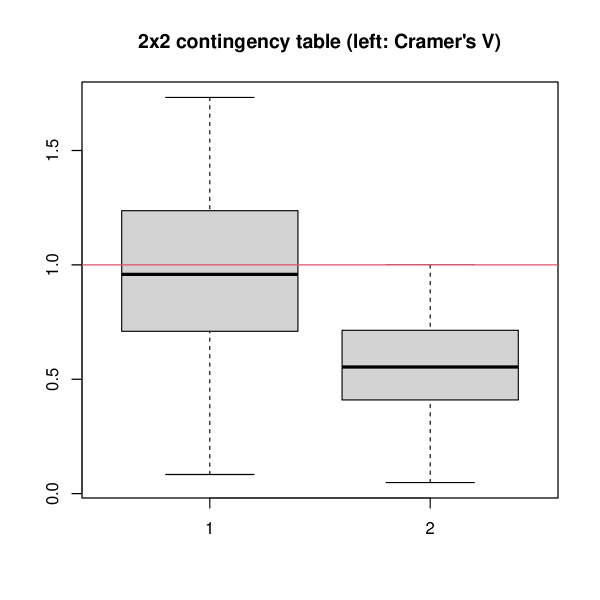
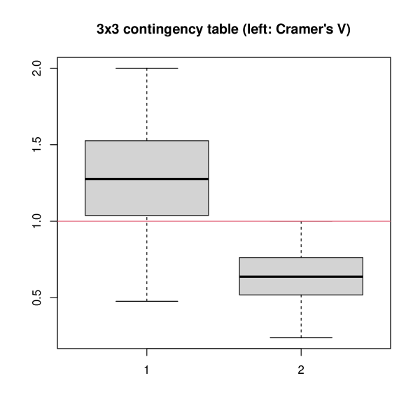
3 Simulation
For two contingency tables, and , for the total number , we randomly generate the number of cells. We assume that the probabilities of the cells are all equal and that the number of simulations is 1000.
| contingency table | contingency table | |||
| V | modified V | V | modified V | |
| Min. | 0.0837 | 0.0483 | 0.4774 | 0.2387 |
| 1st Qu. | 0.7096 | 0.4097 | 1.038 | 0.519 |
| Median | 0.9358 | 0.5403 | 1.2656 | 0.6328 |
| Mean | 0.9815 | 0.5667 | 1.2874 | 0.6437 |
| 3rd Qu. | 1.2369 | 0.7141 | 1.5263 | 0.7632 |
| Max. | 1.7321 | 1 | 2 | 1 |
Ginwidth=0.45
4 Conclusion
The proof and simulation results regarding the maximum clearly show that we need to modify the Cramér’s V. The previous contingency coefficients must be modified by using a modified Cramér’s V with the maximum value .
Acknowledgment. This paper was partially supported by Grant-in-Aid for Scientific Research (C) (general) 22K11946 from the Ministry of Education, Culture, Sports, Science and Technology of Japan.
References
- [1] Haldun Akoglu, User’s guide to correlation coefficients, Turkish Journal of Emergency Medicine, 18, 91–93, 2018.
- [2] Harald Cramér, Mathematical methods of statistics, Princeton University Press, 1946.
- [3] Charles C. Okeke, Alternative methods of solving biasedness in Chi-square contingency table, Academic Journal of Applied Mathematical Sciences, 5(1), 1–6, 2019.
- [4] Wataru Urasaki, Tomoyuki Nakagawa, Tomotaka Momozaki, and Sadao Tomizawa, Generalized Cramér’s coefficient via -divergence for contingency tables, Advances in Data Analysis and Classification, 18, 893–910, 2024.