Video Depth Anything: Consistent Depth Estimation for Super-Long Videos

Abstract

Depth Anything has achieved remarkable success in monocular depth estimation with strong generalization ability. However, it suffers from temporal inconsistency in videos, hindering its practical applications. Various methods have been proposed to alleviate this issue by leveraging video generation models or introducing priors from optical flow and camera poses. Nonetheless, these methods are only applicable to short videos ($\textless$ 10 seconds) and require a trade-off between quality and computational efficiency. We propose Video Depth Anything for high-quality, consistent depth estimation in super-long videos (over several minutes) without sacrificing efficiency. We base our model on Depth Anything V2 and replace its head with an efficient spatial-temporal head. We design a straightforward yet effective temporal consistency loss by constraining the temporal depth gradient, eliminating the need for additional geometric priors. The model is trained on a joint dataset of video depth and unlabeled images, similar to Depth Anything V2. Moreover, a novel key-frame-based strategy is developed for long video inference. Experiments show that our model can be applied to arbitrarily long videos without compromising quality, consistency, or generalization ability. Comprehensive evaluations on multiple video benchmarks demonstrate that our approach sets a new state-of-the-art in zero-shot video depth estimation. We offer models of different scales to support a range of scenarios, with our smallest model capable of real-time performance at 30 FPS.

Figure 1: Left: Our model can generate consistent depth predictions for long videos with rich actions. The demo video shows a 196-second (4690 frames) long take of pair skating, as sourced from [14]. Right: Comparison to baselines in terms of accuracy ($\delta_{1}$), consistency, and latency on the Nvidia A100 GPU (denoted with circle size). Consistency is defined as the maximum Temporal Alignment Error (TAE) among all models minus the TAE of each individual model. Our model achieves the best performance in all aspects.

1 Introduction

Recently, monocular depth estimation (MDE) has made significant progress, as evidenced by advances in depth foundation models [41, 42, 17, 3]. For example, Depth Anything V2 [42] demonstrates a strong generalization ability in producing depth predictions with rich details in various scenarios while being computationally efficient. However, these models have a major limitation: they are mainly designed for static images and suffer from flickering and motion blur in videos. This limitation restricts their applications in robotics [8], augmented reality [12], and advanced video editing [46, 25], which requires temporally consistent depth.

Extensive efforts are being made to address this problem. Early work [18, 21, 47] often relies on test-time optimization to tune a pretrained monocular depth model with sophisticated geometry constraints. Given the heavy overhead at inference time of these methods, recent work mainly focuses on feedforward models and can be categorized into two approaches. The first approach [38] involves designing a plug-and-play module to augment monocular depth model predictions with temporal consistency. The training of such a module is highly dependent on optical flow [39] or camera poses [30] for consistency constraints, making the module susceptible to corresponding errors. The second approach [32, 13, 40] repurposes pre-trained video diffusion models [4] into video-to-depth models. These methods excel at producing fine-grained details, but are computationally inefficient, cannot leverage existing depth foundation models, and can only handle videos with limited length.

Then, a natural question arises: Is it possible to have a model that can perfectly inherit the capabilities of existing foundation models while achieving temporal stability for arbitrarily long videos? In this paper, we show that the answer is YES by developing Video Depth Anything based on Depth Anything V2, without sacrificing its generalization ability, richness in details, or computational efficiency. This target is achieved without introducing any geometric priors or video generation priors.

Specifically, we first design a lightweight spatial-temporal head (STH) to replace the DPT head [28] and enable temporal information interactions. STH includes four temporal attention layers, applied along the temporal dimension for each spatial position. Introducing temporal attention only in the head prevents the learned representation from being corrupted by the limited video data. Then, we propose a temporal gradient matching loss to constrain depth prediction gradients along the temporal dimension to match those calculated from the ground truth. This loss function is jointly optimized with the scale-shift-invariant loss and spatial gradient matching loss [3, 41]. Despite its simplicity, it can effectively boost the model’s temporal consistency. Third, to maintain the original capabilities of the model, we train it jointly on 550K video frames with depth annotations using supervised learning, and on 0.62 million unlabeled images using self-training, similar to Depth Anything V2 [42]. To handle super-long videos at inference time, we developed a novel segment-wise processing strategy. Each new segment is concatenated with eight overlapping frames and two key frames from the previous video clips, forming a total of 32 frames. Then, the overlapping frames will be progressively interpolated between the two consecutive windows to ensure smoothness.

We compare our model with baselines on five datasets for zero-shot video depth estimation. Our model achieves state-of-the-art (SOTA) results on four of the datasets in terms of spatial accuracy and outperforms all baselines on all datasets in terms of temporal consistency. Not only can our model produce depth outputs visually comparable to video-diffusion-based methods, but it is also significantly more computationally efficient. For the first time, we can estimate consistent depth for videos over several minutes (see Fig.˜1). Additionally, we tested our model for zero-shot image depth estimation on five datasets, noting only a marginal performance drop on one dataset compared to Depth Anything V2. As shown in Fig.˜1 (right), our model achieves the best performance in all three aspects: spatial accuracy, temporal consistency, and computational efficiency.

Our contributions are summarized as follows:

• We develop a novel method to transform Depth Anything into Video Depth Anythingfor depth estimation in arbitrarily long videos.

• We propose a simple yet effective loss function that enforces temporal consistency constraints without introducing geometric or generative priors.

• Our model not only sets new SOTA (both spatially and temporally) in video depth estimation but is also the most computationally efficient.

2 Related Work

Monocular depth estimation. Early monocular depth estimation  [9, 10, 1, 45] efforts were primarily trained and tested on in-domain datasets. These models were constrained by the limited diversity of their training data, showing bad generalization for zero-shot application. Subsequently, MiDaS [3] introduced multi-dataset mixed training using an affine-invariant alignment method, significantly enhancing model generalization. However, due to limitations in the backbone model’s performance and noise in the labeled depth data, the resulting depth maps lacked fine details. Following MiDaS [3], monocular depth estimation models have generally bifurcated into two categories: relative depth models that estimate affine-invariant depth (e.g., DPT [28], DepthAnything [41, 42], Marigold [17]) and metric depth models that estimate depth with an absolute scale (e.g., ZoeDepth [2], Metric3D [44], UniDepth [27]). Metric depth models require training with metric depth data that includes camera parameters [44], thus their available training data is more limited compared to affine-invariant depth models, resulting in poorer generalization. Recently, Depth Anything V2 [42] leveraged the Dinov2 [23] pre-trained backbone to train an affine-invariant large-scale model using synthetic data with high-detail fidelity. This large model was then used as a teacher to distill smaller models on 62 million unlabeled datasets [41], achieving SOTA performance in both generalization and geometric details. However, since Depth Anything V2 [42] was trained exclusively on static images, thus lacks temporal consistency.

Consistent video depth estimation. The core task of consistent video depth estimation is to obtain temporal consistent and accuracy depth maps. Early methods for video depth relied on test-time training [21, 18, 47], which were impractical for applications for their low efficiency. In recent years, learning-based models have emerged. Some of these models, such as MAMo [43], use optical flow [33] to warp features, while others [29] depends on relative poses between frames to construct cost volumes. However, their performance were suffered from errors of inaccurate optical flow or pose estimation. Additional approaches have attempted to enhance off-the-shelf monocular depth estimation (MDE) models with temporal stability model blocks  [38]. Nevertheless, these efforts have not achieved satisfactory results due to suboptimal model designs and inadequate geometric consistency constraints. Furthermore, video diffusion models such as ChronoDepth [32], DepthCrafter [13], and DepthAnyVideo[40] show better details and temporal consistency. But they suffered from slow inference speeds and require extensive video depth training data. Limited by the large memory, these models [13] were typically tested only within the maximum window length used during training, leading to depth flickering between windows and poor temporal and spatial consistency in long videos.

3 Video Depth Anything

In this section, we introduce Video Depth Anything, a feed-forward video transformer model to efficiently estimate temporally consistent video depth. We adopt the affine-invariant depth, but share the same scale and shift across the entire video. The pipeline of our method is shown in Fig. 2. Our model is built upon Depth Anything V2 with an additional temporal module and video dataset training (Sec. 3.1). A novel loss to enfoce temporal consistency is proposed in Sec. 3.2. Finally, a strategy combined with overlapping frames and key frames is presented to efficiently support super-long video inference (Sect. 3.3).

Figure 2: Overall pipeline and the spatio-temporal head. Left: Our model is composed of a backbone encoder from Depth Anything V2 and a newly proposed spatio-temporal head. We jointly train our model on video data using ground-truth depth labels for supervision and on unlabeled images with pseudo labels generated by a teacher model. During training, only the head is learned. Right: Our spatiotemporal head inserts several temporal layers into the DPT head, while preserving the original structure of DPT head [28].

3.1 Architecture

Due to the lack of sufficient video depth data, we start with a pre-trained image depth estimation model, Depth Anything V2, and adopt a joint training strategy using both image and video data.

Depth Anything V2 Encoder. Depth Anything V2 [42] is the current state-of-the-art monocular depth estimation model, characterized by its high accuracy and generalization capabilities. We use its trained model as our encoder. To reduce training costs and preserve well-learned features, the encoder is frozen during training.

Unlike monocular depth encoders that only accept image input, our training scenario requires the encoder to process simultaneously both video and image data. To extract features from video frames with an image encoder, we collapse the temporal dimension of a video clip into the batch dimension. The input data are denoted as $\mathbf{X}\in\mathbb{R}^{(B\times N)\times C\times H\times W}$, where $B$ represents the batch size, $N$ is the number of frames in the video clip, $N=1$ for the image as input, $C,H,W$ are the number of channels, height, width of the frames, respectively. The encoder takes $\mathbf{X}$ as input to produce a series of intermediate feature maps $\mathbf{F_{i}}\in\mathbb{R}^{(B\times N)\times(\frac{H}{p}\times\frac{W}{p})\times C_{i}}$, $p$ is the patch size of the encoder. Although the image encoder extracts strong visual representations from individual frames, it neglects the temporal information interactions between frames. Thus, the spatiotemporal head is introduced to model the temporal relationship among the frames.

Spatiotemporal Head. The spatiotemporal head (STH) is built upon the DPT [28] head and with the only modification being the insertion of temporal layers to capture temporal information. A temporal layer consists of a multi-head self-attention [34] model (SA) and a feed-forward network (FFN). When inputting a feature $\mathbf{F_{i}}$ into the temporal layer, the temporal dimension $N$ is isolated, and self-attention is executed solely along the temporal dimension to facilitate the interaction of temporal features. To capture temporal positional relationships among different frames, we utilize absolute positional embedding to encode temporal positional information from the video sequence.

The spatiotemporal head uniformly samples 4 feature maps from $\mathbf{F_{i}}$ (including the final features from the encoder, denoted as $\mathbf{F_{4}}$) as inputs, and predicts a depth map $\mathbf{D}\in\mathbb{R}^{H\times W}$. As shown in Figure 2, the selected features $\mathbf{F_{i}}$ are fed into the Reassemble layer to produce a feature pyramid. Then, the features are gradually fused from low resolution to high resolution by the Fusion layer. The Reassemble and Fusion layer are proposed by DPT [28]. The final fused high-resolution feature maps are passed through the output layer to produce the depth map $\mathbf{D}$. To reduce the additional computational load, we insert the temporal layer at a few positions with lower feature resolutions.

3.2 Temporal Gradient Matching loss

In this section, we start with the Optical Flow Based Warping (OPW) loss, then explore new loss designs and ultimately propose a Temporal Gradient Matching Loss (TGM) that does not rely on optical flow, yet still ensures the temporal consistency of predictions between frames.

OPW loss. To constrain temporal consistency, previous video models such as [38, 19, 37] assume that the depths at corresponding positions in adjacent frames, identified through optical flow, are consistent, e.g., the Optical Flow based Warping (OPW) loss proposed in NVDS [38]. OPW loss is computed after obtaining corresponding points on the basis of optical flow and warping. Specifically, for two consecutive depth prediction results, $p_{i}$ and $p_{i+1}$. $p_{i+1}$ is warped to $\hat{p_{i}}$ according to the wrapping relationship derived from the optical flow, and then the loss is calculated with:

$$\mathcal{L}_{\text{OPW}}=\frac{1}{N-1}\sum_{i=2}^{N}\parallel p_{i}-\hat{p_{i}}\parallel_{1},\vskip-8.53581pt$$ (1)

where $N$ denotes the length of a video window, and $||\cdot||_{1}$ represents $\ell$1 distance. However, there is a fundamental issue with the OPW loss: the depth of corresponding points is not invariant across adjacent frames. This assumption holds true only when adjacent frames are stationary. For instance, in driving scenario, when a car is moving forward, the distance to static objects in front decreases relative to the car, violating the assumption of $\mathcal{L}_{OPW}$. To address this inherent issue of OPW, we propose a new loss function to constrain the temporal consistency of depth.

Temporal gradient matching loss (TGM). When calculating the loss, we do not assume that the depth of the corresponding points in adjacent frames remains unchanged. Instead, we posit that the change in depth of corresponding points between adjacent prediction frames should be consistent with the change observed in ground truth. We refer to this discrepancy as a stable error (SE) given by:

$$\mathcal{L}_{\text{SE}}=\frac{1}{N-1}\sum_{i=1}^{N-1}\parallel\mid\hat{d_{i}}-d_{i}\mid-\mid\hat{g_{i}}-g_{i}\mid\parallel_{1}.\vskip-8.53581pt$$ (2)

Here, $d_{i},g_{i}$ are scaled and shifted versions of the predictions and ground truth. $\hat{d_{i}},\hat{g_{i}}$ denotes the warped depth from the subsequent frame using optical flow. $\mid\cdot\mid$ is used to represent the absolute values.

However, generating optical flow incurs additional overhead. To address the dependence on optical flow, we further generalize the above assumption. Specifically, it is not necessary to use the corresponding points obtained from the optical flow. Instead, we directly use the depth at the same coordinate in adjacent frames to calculate the loss. The assumption is that the change in depth at the same image position between adjacent frames should be consistent with that in the ground truth. Since this process is akin to calculating the gradient of values in temporal dimension, we name it Temporal Gradient Matching Loss, as given by

$$\mathcal{L}_{\text{TGM}}=\frac{1}{N-1}\sum_{i=1}^{N-1}\parallel\mid d_{i+1}-d_{i}\mid-\mid g_{i+1}-g_{i}\mid\parallel_{1}.\vskip-8.53581pt$$ (3)

In practice, we only compute the TGM loss in regions where the change in ground truth depth, i.e., $\mid g_{i+1}-g_{i}\mid<0.05$. This threshold helps to avoid sudden changes in depth map caused by edges, dynamic objects, and other factors that introduce unsteadiness during training.

Our total loss to supervise video depth data is as follows:

$$\mathcal{L}_{\text{all}}=\alpha\mathcal{L}_{\text{TGM}}+\beta\mathcal{L}_{\text{ssi}},\vskip-8.53581pt$$ (4)

where $\mathcal{L}_{ssi}$ is a scale- and shift-invariant loss to supervise single images proposed by MiDaS [3]. $\alpha$ and $\beta$ are weights to balance spatio-temporal consistency and spatial structure in a single frame.

3.3 Inference strategy for super-long sequence

Figure 3: Inference strategy for long videos. $N$ is the video clip lenght consumed by our model. Each inference video clip is built by $N-T_{o}-T_{k}$ future frames, $T_{o}$ overlapping/adjacent frames, and $T_{k}$ key frames. The key frames are selected by taking every $\Delta_{k}$-th frame going backward. Then, the new depth predictions will be scale-shift-aligned to the previous frames based on the $T_{k}$ overlapping frames. We use $N=32,T_{o}=8,T_{k}=2,\Delta_{k}=12$.

To handle videos of arbitrary length, a straightforward approach is simply to concatenate the model outputs from different video windows. However, this method fails to ensure smooth transitions between windows. A more sophisticated technique entails inferring video windows with overlapping regions. By utilizing the predicted depth of the overlapping regions to compute an affine transform, predictions from one window can be aligned with those from another. Nevertheless, this method can introduce accumulated errors through successive affine alignments, leading to depth drift in extended videos. To address these challenges in ultra-long videos with a limited inference window size, we proposed key-frame referencing to inherit scale and shift information from past predictions and overlapping interpolation to ensure smooth inference across local windows.

Key-frame referencing. As illustrated in  Fig.˜3, a subsequent video clip for inference is composed of three parts: $N-T_{o}-T_{k}$ future frames, $T_{o}$ overlapping frames from the previous clip and $T_{k}$ key frames. The key frames are subsampled from the previous frames with an interval of size $\Delta_{k}$. Therefore, the video clip to be consumed share the same length as during training. This approach incorporates content from earlier windows into the current window with minimal computation burden. According to our experiment results, such simple strategy can significantly reduce accumulated scale drift, especially for long video.

Depth clip stitching. Using $T_{o}$ overlapping frames (in  Fig.˜3) between two consecutive windows is crucial for avoiding flickering depth predictions. The effects of overlapping frames are twofold. First, by sharing partial frame features, the scale and shift across consecutive windows will be more similar. Second, the depth prediction for the overlapping frames is updated by interpolating between the two segments. Assume the depth for the $o_{i}$-th overlapping frame from the previous segment is denoted by $\mathbf{D}_{o_{i}}^{\text{pre}}$, and the depth from the current segment is denoted by $\mathbf{D}_{o_{i}}^{\text{cur}}$. The final depth is updated as $\mathbf{D}_{o_{i}}=\mathbf{D}_{o_{i}}^{\text{pre}}\cdot w_{i}+\mathbf{D}_{o_{i}}^{\text{cur}}\cdot(1-w_{i})$, where $w_{i}$ linearly decays from 1 to 0 as $i$ increases from 1 to $T_{o}$.

4 Experiments

Method / Metrics	KITTI [11]		Scannet [7]		Bonn [24]		NYUv2 [22]		Sintel [5](~50 frames)		Scannet (170 frames[40])	$\delta_{1}$ Rank
	AbsRel (↓)	$\delta_{1}$ (↑)	AbsRel (↓)	$\delta_{1}$  (↑)	AbsRel (↓)	$\delta_{1}$  (↑)	AbsRel (↓)	$\delta_{1}$  (↑)	AbsRel (↓)	$\delta_{1}$  (↑)	TAE (↓)
DAv2-L [42]	0.137	0.815	0.150	0.768	0.127	0.864	0.094	0.928	0.390	0.541	1.140	3.6
NVDS [38]	0.233	0.614	0.207	0.628	0.199	0.674	0.217	0.598	0.408	0.464	2.176	6.8
NVDS [38] + DAv2-L [42]	0.227	0.617	0.194	0.658	0.191	0.700	0.184	0.679	0.449	0.503	2.536	5.8
ChoronDepth [32]	0.243	0.576	0.199	0.665	0.199	0.665	0.173	0.771	0.192	0.673	1.022	5.2
DepthCrafter [13]	0.164	0.753	0.169	0.730	0.153	0.803	0.141	0.822	0.299	0.695	0.639	3.4
DepthAnyVideo [40]	-	-	-	-	-	-	-	-	0.405	0.659	0.967	-
VDA-S (Ours)	0.086	0.942	0.110	0.876	0.083	0.950	0.077	0.959	0.339	0.584	0.703	2.6
VDA-L (Ours)	0.083	0.944	0.089	0.926	0.071	0.959	0.062	0.971	0.295	0.644	0.570	1.6

Table 1: Zero-shot video depth estimation results. We compare with representative single-image [42] and video depth estimation models [38, 32, 13, 40]. “VDA-S” denotes our model with ViT-Small backbone. “VDA-L” denotes our model with ViT-Large backbone. The best and the second best results are highlighted.

Method / Metrics	KITTI		Sintel		NYUv2		ETH3D		DIODE		$\delta_{1}$ Rank
	AbsRel (↓)	$\delta_{1}$  (↑)	AbsRel (↓)	$\delta_{1}$  (↑)	AbsRel (↓)	$\delta_{1}$  (↑)	AbsRel (↓)	$\delta_{1}$  (↑)	AbsRel (↓)	$\delta_{1}$  (↑)
DepthCrafter [13]	0.107	0.891	0.568	0.652	0.082	0.936	0.179	0.793	0.141	0.857	4
DepthAnyVideo [40]	0.073	0.946	0.687	0.692	0.058	0.963	0.123	0.881	0.072	0.942	2.4
DAv2-L [42]	0.074	0.946	0.487	0.752	0.045	0.979	0.131	0.865	0.066	0.952	1.4
VDA-L (Ours)	0.075	0.946	0.496	0.754	0.046	0.978	0.132	0.863	0.067	0.950	2

Table 2: Zero-shot single-image depth estimation results. We compare with representative single-image [42] and video depth estimation models [13, 40] with single-frame inputs. “VDA-L” denotes our model with ViT-Large backbone. The best and the second best results are highlighted.

4.1 Evaluation

Datasets. For the quantitative evaluation of video depth estimation, we utilize five datasets that encompass a wide range of scenes, including indoor [7, 22, 24], outdoor [11], and wild environments [5]. Each video is evaluated using up to 500 frames, which is significantly more extensive than the 110 frames used in  [13]. For results with 110 frames, see the appendix for details. In addition to video depth evaluation, we also assess our model’s performance on static images [42] on five image benchmarks  [11, 5, 22, 31, 15].

Metrics. We evaluate our video depth model using both geometric accuracy and temporal stability metrics. In accordance with  [13], we first align the predicted depth maps with the ground truth by applying a uniform scale and shift throughout the video. For geometric accuracy, we compute the Absolute Relative Error (AbsRel) and $\delta_{1}$ metrics  [42, 13]. To assess temporal stability, we use the Temporal Alignment Error (TAE) metric in  [40], to measure the reprojection error of the depth maps between consecutive frames.

4.2 Zero-shot Depth Estimation

We compare our model against four representative video depth estimation models: NVDS [38], ChronoDepth [32], DepthCrafter [13], and DepthAnyVideo [40] on established video depth benchmarks. Furthermore, we introduce two robust baselines, 1) Depth Anything V2 [42] (DAv2), and 2) NVDS + DAv2, i.e., replacing the base model in NVDS with DAv2. It is important to note that DepthAnyVideo [40] supports a maximum of 192 frames per video; therefore, we report metrics for the Sintel [5] dataset exclusively for this model, as other datasets contain videos that exceed this frame limit. For static image evaluation, we compare the performance of our model with DepthCrafter [13], DepthAnyVideo [40], and Depth Anything V2 [42].

Video depth results. As demonstrated in Table 1, our VDA model achieves state-of-the-art performance across all long video datasets, excelling in both geometric and temporal metrics. This underscores the effectiveness of our robust foundation model and the innovative design of our video model. Notably, on the KITTI [11], Scannet [7], and Bonn [24] datasets, our model surpasses other leading methods by a significant margin of approximately $10\%$ in the geometric accuracy metric $\delta_{1}$, although it is trained on much fewer video data compared to DepthCrafter [13] (over 10 million frames) and DepthAnyVideo [40] (6 million frames). For the short video synthetic dataset Sintel [5], where sequences contain around 50 frames each, DepthCrafter [13] exhibits better accuracy than our model. This discrepancy may be attributed to the absence of movie data, which features frames with focal lengths similar to those in Sintel [5], in our model’s training set. It is also worth highlighting that our compact model, VDA-S, which has significantly lower latency compared to other models (as shown in Table 3), demonstrates superior geometric accuracy over representative diffusion-based methods for long videos.

Image depth results. As displayed in Table 2, our video depth model achieves competitive depth metrics compared to DAv2-L [42] in most datasets. This shows that our model maintains the geometric accuracy of the foundation model while also ensuring video stabilization.

Long video quantitative results. We selected 10 scenes each from Bonn [24] and Scannet [7], and 8 scenes from NYUv2 [22], with each scene comprising 500 video frames. We then evaluated the video depth at frame lengths of 110, 192, 300, 400, and 500, where 110 and 192 correspond to the maximum window sizes of DepthCrafter [13] and DepthAnyVideo [40], respectively. The variation in metrics is shown in Figure 4. As illustrated, our model significantly outperforms DepthCrafter [13] in all evaluated frame lengths for all datasets, exhibiting minimal metric degradation as the number of frames increases. Furthermore, our model surpasses DepthAnyVideo [40] in Scannet [7] and NYUv2 [22], and achieves comparable results in Bonn [24] for the 110 and 192 frame metrics. Most notably, our approach supports inference for arbitrarily long videos, providing a substantial advantage in practical applications.

Figure 4: Video depth estimation accuracy for different frame length. We compare our model (VDA-L) with DepthCrafter [13] and DepthAnyVideo [40] from 110 to 500 frames on Bonn [24], Scannet [7], and NYUv2 [22].

Qualitative results. We present two results of the long video visualization in 5. The second column represents image temporal profiles obtained by slicing images along the timeline at the red-line positions. The subsequent columns represent the corresponding depth profiles. The red boxes highlight instances where the depth profile of our model more closely resembles the ground truth (GT) compared to DepthCrafter [13], indicating superior geometric accuracy. Furthermore, our model demonstrates better temporal consistency, as shown in the blue boxes. In these instances, DepthCrafter [13] exhibits drifted depth, and DAv2-L [42] produces flickering depth.

Figure 5: Qualitative comparison for real-world long video depth estimation. We compare our model with DAv2-L [42] and DepthCrafter [13] on 500-frame videos from Scannet [7] and Bonn [24].

In addition to long videos, we present in-the-wild short video results in Figure 6. Depth Any Video [40] exhibits depth inconsistency even within a single reference window, as indicated by the blue boxes. Although DepthCrafter [13] demonstrates smoother depth along video frames compared to Depth Any Video [40], it fails to estimate accurate depth in some complex environments.

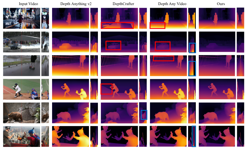
Figure 6: Qualitative comparison for in-the-wild short video depth estimation. We compare with Depth-Anything-V2 [42], DepthCrafter [13] and DepthAnyVideo [40] on videos with less than 100 frames from DAVIS [26]. Red boxes show incorrect depth estimation while blue boxes show inconsistent depth estimation.

Inference time. We measure the inference latency of various models on an A100 GPU. As shown in Table 3, our large model achieves the lowest inference time compared to both diffusion-based methods (DepthAnyVideo [40] and DepthCrafter [13]) and the transformer-based method (NVDS [38]). This performance is attributed to our feed-forward transformer structure and lightweight temporal modules. Notably, the latency of our large model, VDA-L, is only approximately $10\%$ greater than that of DAv2-L [42, 13], which uses the same encoder structure, thus demonstrating the efficiency of our spatiotemporal head. Furthermore, the inference latency of our small model is less than 10ms, indicating its potential for real-time applications.

Method	Precision	Latency (ms)
ChronoDepth	FP16	506
DepthCrafter	FP16	910
DepthAnyVideo	FP16	159
NVDS	FP32	204
DAv2-L	FP32	60
VDA-L (Ours)	FP32	67
VDA-S (Ours)	FP32	9.1

Table 3: Inference latency comparisons for video depth estimation. We measure average runtime for each frame on a single A100 GPU with a resolution of $518\times 518$.

4.3 Ablation Studies

Througout this section, we use the VDA-S model with a window size of 16, trained without image distillation unless otherwise specified. The metrics reported without a dataset name represent the mean values across all datasets.

Temporal Loss. Temporal loss experiments are conducted on the TartanAir [36] and VKITTI [6] datasets. In addition to the TGM+SSI loss we proposed, we evaluate the performance of three other loss functions. The VideoAlign loss is a straightforward design that aligns predicted video depth to the ground truth using a shared scale-shift and computes the $l1$ loss. Building upon VideoAlign, the VideoAlign+SSI loss introduces an additional spatial loss to supervise the single-frame structure. The OPW+SSI loss combines optical flow-based warping loss proposed in [38] with a single-frame spatial loss. SE refers to the stable error loss introduced in Equation 2. As shown in Table 4, while VideoAlign and VideoAlign+SSI exhibit good geometric metrics, their video stability metrics are poor. Among loss functions with temporal constraints, our proposed TGM+SSI loss significantly outperforms the OPW+SSI loss on both geometric and stability metrics, and achieves metrics comparable to SE+SSI. It shows that TGM not only corrects the errors from OPW but also eliminates the dependency on optical flow.

Loss	AbsRel (↓)	$\delta_{1}$  (↑)	TAE (↓)
VideoAlign	0.151	0.846	1.326
VideoAlign+SSI	0.151	0.848	1.207
OPW [38]+SSI	0.182	0.771	0.918
SE+SSI	0.160	0.836	0.753
TGM+SSI (Ours)	0.166	0.832	0.767

Table 4: Ablation studies on the effectiveness of the temporal losses. “VideoAlign” denotes the spatial loss with a shared scale-shift alignment applied to the entire video. “SSI” is the image-level spatial loss used in [42]. “OPW” refers to the optical flow-based warping loss described in [38]. “SE” refers to the stable error as introduced in Equation 2. “TGM” represents our proposed temporal gradient matching loss.

Inference Strategies. To ablate our inference strategy, we consider four different inference schemes. Baseline, inference is performed independently on each window without overlapping frames. Overlap Alignment (OA), based on scale-shift invariant alignment of the overlapping frames between two neighboring windows, this method stitches the two windows together. Overlap Interpolation (OI), following the approach in DepthCrafter [13], this method splices two windows together after performing linear interpolation in the overlap region. Overlap Interpolation + KeyFrame Reference (OI+KR), on the basis of OI, we additionally introduce key frames from the previous window as a reference for the current inference. As shown in Table 5, OA achieves metrics comparable to those of OI+KR. However, it leads to cumulative scale drift during long video inference. This issue is illustrated in Figure 7, where we evaluate OA and OI+KR on an extended video with a duration of $4^{\prime}04^{\prime\prime}$. Notably, the red boxed region in the last frame of the video processed by OA highlights a cumulative drift in the depth scale. In contrast, OI+KR maintains global scale consistency more effectively throughout the duration of the video. One possible explanation for the better metrics of OA in the evaluation datasets is that the 500-frame evaluation video dataset is not long enough to reflect the scale drift issues encountered in real-world, long-duration videos.

Window sizes. As shown in Table 5, the model with a window size of 32 exhibits better geometric accuracy and temporal consistency compared to the model with a window size of 16. However, increasing the window size beyond 32 does not yield additional benefits. Given that a larger window size requires more resources for both training and inference, we select a window size of 32 for our final model.

Strategy	Window	AbsRel (↓)	$\delta_{1}$  (↑)	TAE (↓)
Baseline	16	0.157	0.826	0.874
OA	16	0.146	0.845	0.792
OI	16	0.157	0.826	0.783
OI+KR(Ours)	16	0.145	0.849	0.761
OI+KR(Ours)	32	0.144	0.851	0.718
OI+KR(Ours)	48	0.143	0.852	0.732

Table 5: Ablation studies on the effectiveness of different inference strategies and window sizes. “Baseline” denotes directly inference for video clips without overlapping. “OA” denotes inference with a overlap of 4 frames and perform scale-shift alignment across windows. “OI” denotes depth clip stitching with a overlap of 4 frames. “OI+KR” combines the “OI” with our proposed key-frame referencing with extra 2 key-frames.

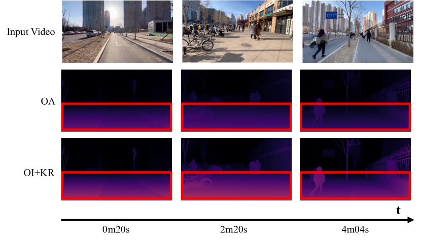
Figure 7: Qualitative comparisons of different inference strategies. We compare overlap alignment (OA) with our proposed overlap interpolation and key-frame referencing (OI + KR) on a self-captured video with 7320 frames.

Training Strategies. In addition to training on synthetic datasets, we conduct an ablation study of distillation training strategies by incorporating an equal amount of pseudo-labeled real datasets. As shown in Table 6, the inclusion of real single-frame datasets in the distillation training process results in a notable enhancement of single-frame depth metrics in both AbsRel and $\delta_{1}$. Furthermore, it also improves video depth metrics.

Datasets	Image-datasets		Video-datasets
	AbsRel (↓)	$\delta_{1}$ (↑)	AbsRel (↓)	$\delta_{1}$ (↑)	TAE (↓)
Video	0.180	0.876	0.145	0.849	0.761
Video + Image	0.167	0.883	0.142	0.852	0.742

Table 6: Ablation studies on the effectiveness of the image dataset distillation. “Video” denotes training using only video datasets. “Video + Image” merges video and image datasets for training using image-level distillation [42].

5 Conclusion

In this paper, we present a novel method named Video Depth Anythingfor estimating the depth of the video that is temporally consistent. The model is built on top of Depth Anything V2 and is based on three key components. First, a spatial-temporal head to involve temporal interactions by applying a temporal self-attention layer to feature maps. Second, a simple temporal gradient matching loss function is used to enforce temporal consistency. Third, to enable long-video depth estimation, a novel keyframe-based strategy is developed for segment-wise inference along with a depth stitching method. Extensive experiments show that our model achieves state-of-the-art performance in three aspects: spatial accuracy, temporal consistency, and computational efficiency. Consequently, it can produce high-quality depth predictions for videos lasting several minutes.

Supplementary Material

1 More Qualitative Results

We present more qualitative comparisons among different approaches for static images and evaluation videos.

In-the-wild image results.

Static image depth estimation results are shown in Fig. 8. DepthCrafter [13] and Depth Any Video [40] exhibit poor performance on oil paintings. DepthCrafter [13] also struggles with transparent objects such as glass and water. Compared with these methods, our model demonstrates superior depth estimation results in complex scenarios. Moreover, our model shows depth estimation results for static images that are comparable to those of Depth-Anything-V2 [42], demonstrating that we have successfully transformed Depth-Anything-V2 into a video depth model without compromising its spatial accuracy.

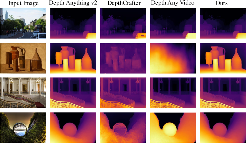
Figure 8: Qualitative comparison for static image depth estimation. We compare our model with Depth-Anything-V2 [42], DepthCrafter [13], and Depth Any Video [40] on static image depth estimation. Our model demonstrates visualization results comparable to those of Depth-Anything-V2 [42].

Evaluation video results.

We showcase five video visualization results from the evaluation datasets Scannet [7] and Bonn [24] in Fig. 9. For enhanced visualization, all predicted video depths are aligned to the ground truth video depths using the same method as in the evaluation. DepthCrafter [13] exhibits depth drift in long videos, as indicated by the blue boxes. Moreover, our model demonstrates superior depth accuracy compared to DepthCrafter [13], as highlighted in the red boxes.

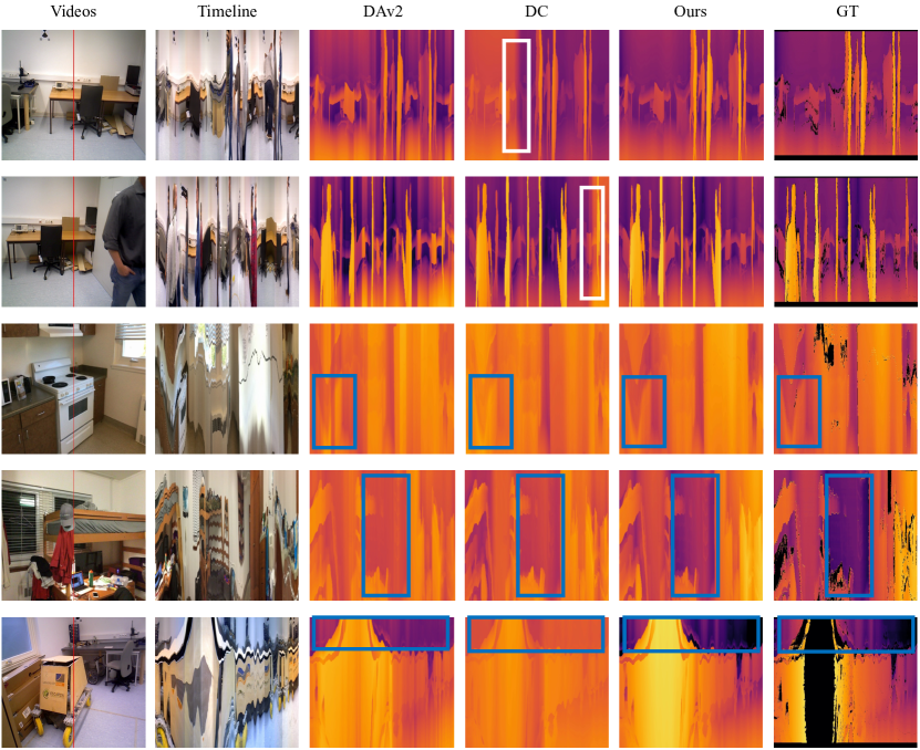
Figure 9: Qualitative comparison for real-world long video depth estimation. We compare with Depth-Anything-V2 [42] and DepthCrafter [13] on 500-frames videos from Scannet [7] and Bonn [24] . We show changes in color and depth over time at the vertical red line in videos. White boxes show inconsistent estimation. Blue boxes show our algorithm has higher accuracy.

2 Short video depth quantitative results

We compare our model with DepthCrafter [13] and Depth Any Video [40] on the KITTI [11], Bonn [24], and Scannet [7] datasets, with frame lengths of 110, 110, and 90, respectively, corresponding to the settings in [13]. As shown in Tab. 7, our model demonstrates a significant advantage of approximately 7% over both DepthCrafter [13] and Depth Any Video [40] on the Scannet dataset [7]. On the KITTI dataset [11], our model significantly outperforms DepthCrafter [13] by about 7%. Additionally, our model achieves comparable results on Bonn [24] and KITTI [11] compared to Depth Any Video [40]. It is worth noting that the parameters of our model and the video depth data used for training are significantly smaller than those of DepthCrafter [13] and Depth Any Video [40], demonstrating the effectiveness and efficiency of our method.

Method / Metrics	Params(M)	# Video Training Data(M)	KITTI(110) [11]		Bonn(110) [24]		Scannet(90) [7]
			AbsRel (↓)	$\delta_{1}$ (↑)	AbsRel (↓)	$\delta_{1}$  (↑)	AbsRel (↓)	$\delta_{1}$  (↑)
DepthCrafter	2156.7	10.5~40.5	0.111	0.885	0.066	0.979	0.125	0.848
DepthAnyVideo	1422.8	6	0.073	0.957	0.051	0.981	0.112	0.883
VDA-L (Ours)	381.8	0.55	0.079	0.950	0.053	0.972	0.075	0.954

Table 7: Zero-shot short video depth estimation results. We compare with DepthCrafter [13] and DepthAnyVideo [40] in short video depth benchmark. “VDA-L” denotes our model with ViT-Large backbone. The default inference resolution of our model is set to 518 pixels on the short side, maintaining the aspect ratio. The best and the second best results are highlighted.

3 Limitations and future work

Our model is trained on publicly available video depth datasets without specially curating data, which may limit its capabilities due to the data quantity. We believe that with more data, the model’s performance can be further improved, and the backbone network can be unlocked for fine-tuning. Additionally, although our model is significantly more computationally efficient than the baselines, it still faces challenges in handling streaming videos, which we leave as future work.

4 More Details of Pipeline

Spatiotemporal head details.

Among the four temporal layers, two are inserted after the Reassemble layers at the two smallest resolutions, and the other two are inserted before the last two Fusion layers.

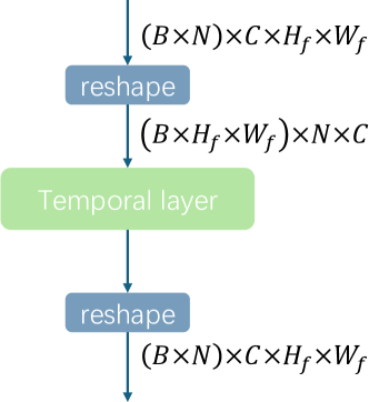
Figure 10: Temporal layer. The feature shape is adjusted for temporal attention.

The shape of the feature is transformed into $(B\times H_{f}\times W_{f})\times N\times C$ before each temporal layer and is transformed back to $(B\times N)\times C\times H_{f}\times W_{f}$ after each temporal layer. Here, $B$ denotes the batch size, $N$ represents the number of frames in the video clip, $H_{f}$ and $W_{f}$ are the height and width of the feature, respectively, and $C$ represents the number of channels in the feature, as shown in Fig. 10

Image distillation details.

We follow the approach in [42] and use a teacher model that comprises a ViT-giant encoder and is trained on synthetic datasets. The loss function used for distillation is identical to the spatial loss employed for video depth data.

Training dataset details.

For video training, we utilize four synthetic datasets with precise depth annotations: TartanAir [36], VKITTI [6], PointOdyssey [48], and IRS [35], totally 0.55 million frames. The TartanAir [36], VKITTI [6], PointOdyssey [48], and IRS [35] datasets contain 0.31M, 0.04M, 0.1M, and 0.1M frames, respectively. Additionally, 0.18 million frames from wild binocular videos labeled with [16] are included for training. We also incorporate a subset of real-world unlabeled datasets from [42] for single image supervision, totaling 0.62 million frames. Notably, we excluded 0.13M frames from PointOdyssey [48] that do not contain background depth ground truth, resulting in our usage of only half of the original dataset. Due to the uneven data distribution across the four training datasets, we employ a uniform sampler to ensure that each dataset contributes equally during training.

Implementation Details

The weights are initialized from Depth Anything V2 [42]. Training comprises two stages. In the first stage, synthetic and wild binocular data are used. In the second stage, synthetic videos and unlabeled single images are employed. Besides the loss defined in Equation 4 used for synthetic videos, unlabeled single images are supervised using the same method as described in [42]. During training, we uniformly sample video clips of 32 frames from each dataset, resize the shorter edge of images to 518 pixels, and perform random center cropping, resulting in training clips with a resolution of $518\times 518\times 32$. We use the AdamW [20] optimizer with a cosine scheduler, setting the base learning rate to $1e^{-4}$. The batch size is set to 16 for video frames, each with a length of 32 frames, and 128 for image datasets. The loss weights for the single frame loss, TGM loss, and distillation loss are set to 1.0, 10.0, and 0.5, respectively.

5 More Details of Evaluation

Evaluation dataset details.

We use a total of five datasets for video depth evaluation: KITTI [11], Scannet [7], Bonn [24], NYUv2 [22], and Sintel [5]. Specifically, we use Scannet [7] and NYUv2 [22] for static indoor scenes, Bonn [24] for dynamic indoor scenes, KITTI [11] for outdoor scenes, and Sintel [5] for wild scenes. For NYUv2 [22], we sample 8 videos from the original dataset, which contains 36 videos. Our evaluation comprises three different settings: long videos, long videos with different frame lengths, and short videos. For the long video evaluation, we use all five datasets and set the maximum frame length to 500 for each video. For the evaluation of long videos with different frame lengths, we select subsets of videos with frame lengths greater than 500 from Scannet [7], Bonn [24], and NYUv2 [22]. For the short video evaluation, we use KITTI [11], Bonn [24], and Scannet [7], setting the maximum frame lengths to 110, 110, and 90, respectively, in accordance with the settings in DepthCrafter [13]. In addition to video depth evaluation, we also assess our model’s performance on static images. Following  [42], we perform evaluations on five image benchmarks: KITTI [11], Sintel [5], NYUv2 [22], ETH3D [31], and DIODE [15]. To ensure a fair comparison, all evaluation videos and images are excluded from the training datasets.

Evaluation metric details.

All video metrics we evaluated are based on ground truth depth. Specifically, we use the least squares method to compute the optimal scale and shift to align the entire inferred video inverse depth with the ground truth inverse depth. The aligned inferred video inverse depth is then transformed into depth, which is subsequently used to compute the video metrics with the ground truth depth. For geometric accuracy, we compute the Absolute Relative Error (AbsRel) and $\delta_{1}$ metrics, following the procedures outlined in  [42, 13]. To assess temporal stability, we use the Temporal Alignment Error (TAE) metric in  [40], to measure the reprojection error of the depth maps between consecutive frames. We use Equation 5.

$$TAE=\frac{1}{2(N-1)} \sum_{k=1}^{N-1}AbsRel(f(\hat{x}_{d}^{k},p^{k}),\hat{x}_{d}^{k+1})+$$ (5)

$$AbsRel(f(\hat{x}_{d}^{k+1},p^{k+1}_{-}),\hat{x}_{d}^{k})$$

Here, $f$ represents the projection function that maps the depth $\hat{x}^{k}_{d}$ from the $k$-th frame to the $(k+1)$-th frame using the transformation matrix $p^{k}$. $p^{k+1}_{-}$ is the inverse matrix for inverse projection. $N$ denotes the number of frames.

Baseline implementations.

We obtain the inferences of DepthCrafter [13], Depth Any Video [40], and NVDS [38] using the respective inference code provided by the authors. Specifically, DepthCrafter [13] employs different inference resolutions for different datasets. Depth Any Video [40] infers with a maximum dimension of 1024. NVDS [38] performs inference on a video twice, with a minimum dimension of 384, once in the forward direction and once in the backward direction, and computes the mean result from these two passes. For Depth-Anything-V2 [42], we obtain the video depth results by inferring each frame individually with a minimum dimension of 518.

6 Applications

Dense point cloud generation.

By aligning single frame with metric depth, which can be obtained from a metric depth model or a sparse point cloud acquired through SLAM, our model can generate a depth point cloud for the entire environment using camera information. The generated point cloud can then be transformed into a mesh and utilized for 3D reconstruction, AR, and VR applications. We present a point cloud generation case in Fig. 12. Here, we sample 10 frames spanning approximately 5 seconds from the KITTI dataset [11]. After obtaining the inferred inverse depth, we compute the global scale and shift by aligning the first frame with the corresponding metric inverse depth. We then apply the affine transformation to the entire set of inverse depth frames and convert them to depth. The final point cloud is generated by merging the point clouds from each frame. As shown in Fig. 12, our model generates a clean and regular point cloud compared to DepthCrafter [13] and Depth Any Video [40].

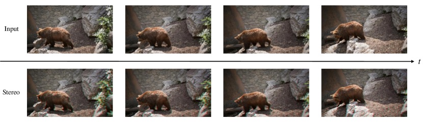
Figure 11: 3D Video Conversion. A video from the DAVIS dataset [26] is transformed into a 3D video using our model.

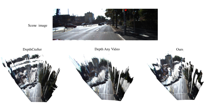
Figure 12: Dense point cloud generation. We compare our model with DepthCrafter [13] and DepthAnyVideo [40] for dense point cloud generation on the KITTI dataset [11]. Our model generates a clean and regular point cloud from multiple frames spanning approximately 5 seconds. In contrast, the point cloud generated by DepthCrafter [13] contains several obvious discontinuous layers. DepthAnyVideo [40] produces a point cloud with numerous noisy outliers and noticeable distortion in distant views.

3D Video Conversion.

Our model can be used to generate 3D videos. Compared to 3D videos generated by monocular depth models, those produced by our video depth model exhibit smoother and more consistent 3D effects. An example is presented in Fig.11.

References

- [1] Shariq Farooq Bhat, Ibraheem Alhashim, and Peter Wonka. Adabins: Depth estimation using adaptive bins. In Proceedings of the IEEE/CVF conference on computer vision and pattern recognition, pages 4009–4018, 2021.
- [2] Shariq Farooq Bhat, Reiner Birkl, Diana Wofk, Peter Wonka, and Matthias Müller. Zoedepth: Zero-shot transfer by combining relative and metric depth. arXiv preprint arXiv:2302.12288, 2023.
- [3] Reiner Birkl, Diana Wofk, and Matthias Müller. Midas v3. 1–a model zoo for robust monocular relative depth estimation. arXiv preprint arXiv:2307.14460, 2023.
- [4] Andreas Blattmann, Tim Dockhorn, Sumith Kulal, Daniel Mendelevitch, Maciej Kilian, Dominik Lorenz, Yam Levi, Zion English, Vikram Voleti, Adam Letts, et al. Stable video diffusion: Scaling latent video diffusion models to large datasets. arXiv preprint arXiv:2311.15127, 2023.
- [5] Daniel J. Butler, Jonas Wulff, Garrett B. Stanley, and Michael J. Black. A Naturalistic Open Source Movie for Optical Flow Evaluation, page 611–625. Jan 2012.
- [6] Yohann Cabon, Naila Murray, and Martin Humenberger. Virtual kitti 2. arXiv preprint arXiv:2001.10773, 2020.
- [7] Angela Dai, Angel X Chang, Manolis Savva, Maciej Halber, Thomas Funkhouser, and Matthias Nießner. Scannet: Richly-annotated 3d reconstructions of indoor scenes. In Proceedings of the IEEE conference on computer vision and pattern recognition, pages 5828–5839, 2017.
- [8] Xingshuai Dong, Matthew A Garratt, Sreenatha G Anavatti, and Hussein A Abbass. Towards real-time monocular depth estimation for robotics: A survey. IEEE Transactions on Intelligent Transportation Systems, 23(10):16940–16961, 2022.
- [9] David Eigen, Christian Puhrsch, and Rob Fergus. Depth map prediction from a single image using a multi-scale deep network. Advances in neural information processing systems, 27, 2014.
- [10] Huan Fu, Mingming Gong, Chaohui Wang, Kayhan Batmanghelich, and Dacheng Tao. Deep ordinal regression network for monocular depth estimation. In Proceedings of the IEEE conference on computer vision and pattern recognition, pages 2002–2011, 2018.
- [11] Andreas Geiger, Philip Lenz, Christoph Stiller, and Raquel Urtasun. Vision meets robotics: The kitti dataset. The International Journal of Robotics Research, 32(11):1231–1237, 2013.
- [12] Aleksander Holynski and Johannes Kopf. Fast depth densification for occlusion-aware augmented reality. ACM Transactions on Graphics (ToG), 37(6):1–11, 2018.
- [13] Wenbo Hu, Xiangjun Gao, Xiaoyu Li, Sijie Zhao, Xiaodong Cun, Yong Zhang, Long Quan, and Ying Shan. Depthcrafter: Generating consistent long depth sequences for open-world videos. arXiv preprint arXiv:2409.02095, 2024.
- [14] Zihao Huang, ShouKang Hu, Guangcong Wang, Tianqi Liu, Yuhang Zang, Zhiguo Cao, Wei Li, and Ziwei Liu. Wildavatar: Web-scale in-the-wild video dataset for 3d avatar creation. arXiv preprint arXiv:2407.02165, 2024.
- [15] Vasiljevic Igor, Kolkin Nicholas, Shanyi Zhang, Ruotian Luo, Haochen Wang, FalconZ. Dai, AndreaF. Daniele, Mohammadreza Mostajabi, Steven Basart, MatthewR. Walter, and Gregory Shakhnarovich. Diode: A dense indoor and outdoor depth dataset. arXiv: Computer Vision and Pattern Recognition,arXiv: Computer Vision and Pattern Recognition, Aug 2019.
- [16] Junpeng Jing, Ye Mao, and Krystian Mikolajczyk. Match-stereo-videos: Bidirectional alignment for consistent dynamic stereo matching. 2024.
- [17] Bingxin Ke, Anton Obukhov, Shengyu Huang, Nando Metzger, Rodrigo Caye Daudt, and Konrad Schindler. Repurposing diffusion-based image generators for monocular depth estimation. In Proceedings of the IEEE/CVF Conference on Computer Vision and Pattern Recognition, pages 9492–9502, 2024.
- [18] Johannes Kopf, Xuejian Rong, and Jia-Bin Huang. Robust consistent video depth estimation. In Proceedings of the IEEE/CVF Conference on Computer Vision and Pattern Recognition, pages 1611–1621, 2021.
- [19] Pengzhi Li, Yikang Ding, Linge Li, Jingwei Guan, and Zhiheng Li. Towards practical consistent video depth estimation. In Proceedings of the 2023 ACM International Conference on Multimedia Retrieval, ICMR ’23, page 388–397, New York, NY, USA, 2023. Association for Computing Machinery.
- [20] I Loshchilov. Decoupled weight decay regularization. arXiv preprint arXiv:1711.05101, 2017.
- [21] Xuan Luo, Jia-Bin Huang, Richard Szeliski, Kevin Matzen, and Johannes Kopf. Consistent video depth estimation. ACM Transactions on Graphics (ToG), 39(4):71–1, 2020.
- [22] Pushmeet Kohli Nathan Silberman, Derek Hoiem and Rob Fergus. Indoor segmentation and support inference from rgbd images. In ECCV, 2012.
- [23] Maxime Oquab, Timothée Darcet, Théo Moutakanni, Huy Vo, Marc Szafraniec, Vasil Khalidov, Pierre Fernandez, Daniel Haziza, Francisco Massa, Alaaeldin El-Nouby, et al. Dinov2: Learning robust visual features without supervision. arXiv preprint arXiv:2304.07193, 2023.
- [24] E. Palazzolo, J. Behley, P. Lottes, P. Giguère, and C. Stachniss. ReFusion: 3D Reconstruction in Dynamic Environments for RGB-D Cameras Exploiting Residuals. 2019.
- [25] Bohao Peng, Jian Wang, Yuechen Zhang, Wenbo Li, Ming-Chang Yang, and Jiaya Jia. Controlnext: Powerful and efficient control for image and video generation. arXiv preprint arXiv:2408.06070, 2024.
- [26] F. Perazzi, J. Pont-Tuset, B. McWilliams, L. Van Gool, M. Gross, and A. Sorkine-Hornung. A benchmark dataset and evaluation methodology for video object segmentation. In Computer Vision and Pattern Recognition, 2016.
- [27] Luigi Piccinelli, Yung-Hsu Yang, Christos Sakaridis, Mattia Segu, Siyuan Li, Luc Van Gool, and Fisher Yu. Unidepth: Universal monocular metric depth estimation. In Proceedings of the IEEE/CVF Conference on Computer Vision and Pattern Recognition, pages 10106–10116, 2024.
- [28] René Ranftl, Alexey Bochkovskiy, and Vladlen Koltun. Vision transformers for dense prediction. In Proceedings of the IEEE/CVF international conference on computer vision, pages 12179–12188, 2021.
- [29] Mohamed Sayed, John Gibson, Jamie Watson, Victor Prisacariu, Michael Firman, and Clément Godard. Simplerecon: 3d reconstruction without 3d convolutions. In European Conference on Computer Vision, pages 1–19. Springer, 2022.
- [30] Johannes L Schonberger and Jan-Michael Frahm. Structure-from-motion revisited. In Proceedings of the IEEE conference on computer vision and pattern recognition, pages 4104–4113, 2016.
- [31] Thomas Schops, Johannes L. Schonberger, Silvano Galliani, Torsten Sattler, Konrad Schindler, Marc Pollefeys, and Andreas Geiger. A multi-view stereo benchmark with high-resolution images and multi-camera videos. In 2017 IEEE Conference on Computer Vision and Pattern Recognition (CVPR), Jul 2017.
- [32] Jiahao Shao, Yuanbo Yang, Hongyu Zhou, Youmin Zhang, Yujun Shen, Matteo Poggi, and Yiyi Liao. Learning temporally consistent video depth from video diffusion priors. arXiv preprint arXiv:2406.01493, 2024.
- [33] Zachary Teed and Jia Deng. Raft: Recurrent all-pairs field transforms for optical flow. In Computer Vision–ECCV 2020: 16th European Conference, Glasgow, UK, August 23–28, 2020, Proceedings, Part II 16, pages 402–419. Springer, 2020.
- [34] A Vaswani. Attention is all you need. Advances in Neural Information Processing Systems, 2017.
- [35] Qiang Wang, Shizhen Zheng, Qingsong Yan, Fei Deng, Kaiyong Zhao, and Xiaowen Chu. Irs: A large naturalistic indoor robotics stereo dataset to train deep models for disparity and surface normal estimation, 2021.
- [36] Wenshan Wang, Delong Zhu, Xiangwei Wang, Yaoyu Hu, Yuheng Qiu, Chen Wang, Yafei Hu, Ashish Kapoor, and Sebastian Scherer. Tartanair: A dataset to push the limits of visual slam. In 2020 IEEE/RSJ International Conference on Intelligent Robots and Systems (IROS), pages 4909–4916. IEEE, 2020.
- [37] Yiran Wang, Zhiyu Pan, Xingyi Li, Zhiguo Cao, Ke Xian, and Jianming Zhang. Less is more: Consistent video depth estimation with masked frames modeling. In Proceedings of the 30th ACM International Conference on Multimedia, MM ’22, page 6347–6358. ACM, Oct. 2022.
- [38] Yiran Wang, Min Shi, Jiaqi Li, Zihao Huang, Zhiguo Cao, Jianming Zhang, Ke Xian, and Guosheng Lin. Neural video depth stabilizer. In Proceedings of the IEEE/CVF International Conference on Computer Vision, pages 9466–9476, 2023.
- [39] Haofei Xu, Jing Zhang, Jianfei Cai, Hamid Rezatofighi, and Dacheng Tao. Gmflow: Learning optical flow via global matching. In Proceedings of the IEEE/CVF conference on computer vision and pattern recognition, pages 8121–8130, 2022.
- [40] Honghui Yang, Di Huang, Wei Yin, Chunhua Shen, Haifeng Liu, Xiaofei He, Binbin Lin, Wanli Ouyang, and Tong He. Depth any video with scalable synthetic data. arXiv preprint arXiv:2410.10815, 2024.
- [41] Lihe Yang, Bingyi Kang, Zilong Huang, Xiaogang Xu, Jiashi Feng, and Hengshuang Zhao. Depth anything: Unleashing the power of large-scale unlabeled data. In CVPR, 2024.
- [42] Lihe Yang, Bingyi Kang, Zilong Huang, Zhen Zhao, Xiaogang Xu, Jiashi Feng, and Hengshuang Zhao. Depth anything v2. arXiv:2406.09414, 2024.
- [43] Rajeev Yasarla, Hong Cai, Jisoo Jeong, Yunxiao Shi, Risheek Garrepalli, and Fatih Porikli. Mamo: Leveraging memory and attention for monocular video depth estimation. In Proceedings of the IEEE/CVF International Conference on Computer Vision, pages 8754–8764, 2023.
- [44] Wei Yin, Chi Zhang, Hao Chen, Zhipeng Cai, Gang Yu, Kaixuan Wang, Xiaozhi Chen, and Chunhua Shen. Metric3d: Towards zero-shot metric 3d prediction from a single image. In Proceedings of the IEEE/CVF International Conference on Computer Vision, pages 9043–9053, 2023.
- [45] Weihao Yuan, Xiaodong Gu, Zuozhuo Dai, Siyu Zhu, and Ping Tan. Neural window fully-connected crfs for monocular depth estimation. In Proceedings of the IEEE/CVF conference on computer vision and pattern recognition, pages 3916–3925, 2022.
- [46] Yabo Zhang, Yuxiang Wei, Dongsheng Jiang, Xiaopeng Zhang, Wangmeng Zuo, and Qi Tian. Controlvideo: Training-free controllable text-to-video generation. arXiv preprint arXiv:2305.13077, 2023.
- [47] Zhoutong Zhang, Forrester Cole, Richard Tucker, William T Freeman, and Tali Dekel. Consistent depth of moving objects in video. ACM Transactions on Graphics (ToG), 40(4):1–12, 2021.
- [48] Yang Zheng, Adam W Harley, Bokui Shen, Gordon Wetzstein, and Leonidas J Guibas. Pointodyssey: A large-scale synthetic dataset for long-term point tracking. In Proceedings of the IEEE/CVF International Conference on Computer Vision, pages 19855–19865, 2023.