DARB-Splatting: Generalizing Splatting with Decaying Anisotropic Radial Basis Functions

Abstract

Splatting-based 3D reconstruction methods have gained popularity with the advent of 3D Gaussian Splatting, efficiently synthesizing high-quality novel views. These methods commonly resort to using exponential family functions, such as the Gaussian function, as reconstruction kernels due to their anisotropic nature, ease of projection, and differentiability in rasterization. However, the field remains restricted to variations within the exponential family, leaving generalized reconstruction kernels largely underexplored, partly due to the lack of easy integrability in 3D to 2D projections. In this light, we show that a class of decaying anisotropic radial basis functions (DARBFs), which are non-negative functions of the Mahalanobis distance, supports splatting by approximating the Gaussian function’s closed-form integration advantage. With this fresh perspective, we demonstrate up to 34% faster convergence during training and a 15% reduction in memory consumption across various DARB reconstruction kernels, while maintaining comparable PSNR, SSIM, and LPIPS results. We will make the code available.

1 Introduction

Splatting plays a pivotal role in modern 3D reconstruction, enabling the representation and rendering of 3D points without relying on explicit surface meshes. The recent 3D Gaussian representation, combined with splatting-based rendering in the 3D Gaussian Splatting (3DGS) [20] has gained widespread attention due to its state-of-the-art (SOTA) visual quality, real-time rendering, and reduction in training times. Since its inception, 3DGS has seen expanding applications in industry, spanning 3D web viewers, 3D scanning, VR platforms, and more, catering to large user bases. As demand continues to rise, so does the need to improve efficiency to conserve computational resources.

Figure 1: This figure compares two different splat functions—Gaussian and cosine (specifically, half-cosine squared)—initialized for the same 3D covariance matrix, $\mathbf{\Sigma}$. Cosine functions, defined as $\cos\left(\frac{d_{M}^{2}}{\xi}\right)$ for $d_{M}^{2}<\frac{\xi\pi}{2}$ where $\xi(>0)$, have finite support and exhibit effective reconstruction performance comparable to Gaussians. Notably, the cosine-based approach enhances training speed by 34% and reduces memory usage by 15%, providing a more memory-efficient alternative.

3DGS represents a 3D scene as a dynamically densified radiance field of 3D Gaussian primitives (ellipsoids) that act as reconstruction kernels. In theory, these ellipsoids are integrated along the projection direction onto the 2D image plane, resulting in 2D Gaussians or splats, a function known as the footprint function or splatting function. This process exploits an interesting property of Gaussians: $2\times 2$ covariance matrix of the 2D Gaussian can be obtained by skipping the third row and column of the $3\times 3$ covariance matrix of the 3D Gaussian [73]. This bypasses costly integration and efficiently simplifies the rendering in practical implementation. The footprint function then models the spread of each splat’s opacity, eventually contributing to the final pixel color. This Gaussian-based blending effect—a smooth, continuous interpolation between splats—inspires the method’s name, “3D Gaussian Splatting.” Numerous subsequent papers [70, 26, 8, 7, 64] build upon this principle, thereby restricting to exponential family functions (e.g., Gaussian functions) to spread each sample in image space.

In splatting, the Gaussian kernel is commonly used, with some variations within the exponential family (e.g., super-Gaussian [15], half-Gaussian [29], Gaussian-Hermite [69] kernels). However, classical signal processing and sampling theory establish that while Gaussians are useful, they are not the most effective interpolators. Especially when determining the pixel color, as in 3DGS, we argue that the Gaussian function may not be the only possible interpolator. We see other functions outperforming them in various contexts, with a notable example being JPEG compression [56, 49], which leverages Discrete Cosine Transforms (DCTs) instead of Gaussians functions for image representation. Additionally, Saratchandran et al. [44] demonstrate that the $\mathrm{sinc}$ activation surpasses $\mathrm{Gaussian}$ activation in implicit neural representations [34, 51, 21, 18], while also suggesting several alternative activation functions. This raises the question: Should we limit ourselves to Gaussians or the exponential family alone? This remains an underexplored area in the computer vision community, partly because costly integration processes make it computationally inefficient to use functions outside of Gaussians.

To address this shortcoming, we generalize these kernels by introducing a broader class of functions, namely, Decaying Anisotropic Radial Basis Functions (DARBFs) that are non-negative (e.g., modified raised cosine, half-cosine, sinc functions and etc.) that include but are not limited to exponential functions. These non-negative DARBFs achieve comparable reconstruction quality while significantly improving training time, along with modest reductions in memory usage (e.g., half-cosine squares in Table 3 and Fig. 1). These DARBFs support anisotropic behavior as they rely on the Mahalanobis distance, and are differentiable, thereby supporting differentiable rendering (Sec. 3.1). A key innovation in our approach is a novel correction factor that preserves the computational efficiency of 3DGS even with alternative kernels by approximating the Gaussian’s closed-form integration shortcut. This allows for effective splatting, yielding novel views, along with subtle improvements in visual quality for some functions (e.g., raised cosines in Fig. 5). To the best of our knowledge, our method represents one of the first modern generalizations expanding splatting to non-exponential functions, and offering high-quality rendering as splatting techniques scale to repetitive industrial applications, where computational savings are increasingly critical.

The contributions of our paper are as follows:

• We present a unified approach where the Gaussian function is merely a special case within the broader class of DARBFs, which can be splatted.

• We leverage the DARBF family, and demonstrate reconstruction kernels achieving up to 34% faster convergence, a 15% reduced memory footprint with on-par PSNR, and enhanced visual quality with finer details in some kernels.

• We introduce a computationally feasible method to approximate the Gaussian closed-form integration advantage when implementing alternative kernels, facilitated by our novel correction factor along with CUDA-based backpropagation codes.

(a) $\exp\left(-\left|\frac{x-\mu}{\sigma}\right|^{\beta}\right)$

$\cos\left(\left(\frac{\mathbf{x-\mu}}{\sigma}\right)^{\beta}\right)$

$\frac{1}{2}+\frac{1}{2}\cos\left(\left(\frac{\mathbf{x-\mu}}{\sigma}\right)^{\beta}\right)$

$\left|{\sin\left(\left(\frac{\mathbf{x-\mu}}{\sigma}\right)^{\beta}\right)}/{\left(\frac{\mathbf{x-\mu}}{\sigma}\right)^{\beta}}\right|$

$\frac{1}{\left[\left|\frac{{x-\mu}}{\sigma}\right|^{\beta}+1\right]^{1/2}}$

Figure 2: Overview of decaying anisotropic radial basis functions (DARBFs) and their respective 1D curves. These functions decay with distance and vary in their sensitivity to direction, making them effective for capturing anisotropic features in spatial data.

2 Related Work

Radiance Field Representation. Light fields [28, 14] were the foundation of early Novel View Synthesis (NVS) techniques capturing radiance in static scenes. The successful implementation of Structure-from-Motion (SfM) [50] enabled NVS to use a collection of images to capture real-world details that were previously impossible to model manually using meshes. This led to the development of the efficient COLMAP pipeline [45], which is now widely utilized in 3D reconstruction to generate initial camera poses and sparse point clouds (e.g., [34, 20, 71, 16]).

Radiance field methods, notably Neural Radiance Fields (NeRFs) [34], utilize neural networks to model radiance as a continuous function in space, thereby enabling NVS. NeRF techniques generate photorealistic novel views [1, 2, 3, 54, 35, 33] through volumetric rendering, integrating color and density along rays. Recent advancements in NeRF improve training [67, 36, 6, 61] and inference times [31, 30, 40, 41, 13]; introduce depth-supervised NeRFs [43, 10] and deformable NeRFs [38, 39, 72, 37]; and enable scene editing [46, 32, 52, 63], among other capabilities. While 3DGS follows a similar image formation model to NeRFs, it diverges by using point-based rendering over volumetric rendering. This approach, leveraging anisotropic splatting, has rapidly integrated into diverse applications within a year’s span, with recent work excelling [11] in physics-based simulations [23, 53, 59, 60], manipulation [7, 27, 19, 47, 68], generation [66, 55, 42, 9] and perception [48, 64, 62], among other areas. Similar to 3DGS, our approach follows point-based rendering but does not restrict points to being represented as 3D Gaussians, as Saratchandran et al. [44] demonstrate for NeRFs. Instead, we provide DARBFs, a class of functions to choose from to represent all points.

Splatting. Splatting, introduced by Westover [57], enables point-based rendering of 3D data, such as sparse SfM points [50] obtained from the COLMAP pipeline [45], without requiring mesh-like connectivity. Each particle’s position and shape are represented by a volume [57] that serves as a reconstruction kernel [73], which is projected onto the image plane through a “footprint function,” or “splat function,” to spread, or splat each particle’s intensity and color across a localized region. Early splatting techniques [58] commonly used spherical kernels for their radial symmetry to simplify calculations, although they struggled with perspective projections. To address this, elliptical kernels [58, 73], projecting elliptical footprints on the image plane were used to better approximate elongated features through anisotropic properties, ultimately enhancing rendering quality. Westover [58], further experimented with different reconstruction kernels, namely $\mathrm{sinc}$, $\mathrm{cone}$, $\mathrm{Gaussian}$, and $\mathrm{bilinear}$ functions without focusing on a specific class of functions. EWA Splatting [73] further refined this approach by selecting a Gaussian reconstruction kernel in 3D, which projects as an elliptical Gaussian footprint on the image plane.

This laid the groundwork for 3DGS to select the Gaussian function. Although the Gaussian function has been extensively used to produce results in the past, other anisotropic radial basis functions exist that can serve as splats, but they lack exploration.

Reconstruction Kernel Modifications. Although 3DGS claims SOTA performance, recent work has shown further improvements by refining the reconstruction kernel. For instance, GES [15] introduces the generalized exponential function, or super Gaussian, by incorporating a learnable shape parameter for each point. However, GES does not modify the splatting function directly within the CUDA rasterizer; instead, it only approximates its effects by adjusting the scaling matrix and loss function in PyTorch, failing to fully demonstrate its superiority [69]. In contrast, we directly modify the CUDA rasterizer’s splatting function to support various DARBFs, achieving superior performance in specific cases compared to 3DGS.

Concurrent work such as 3D-HGS [29], splits the 3D Gaussian reconstruction kernel into two halves, but this approach introduces additional parameters into the CUDA rasterizer, leading to increased computational costs. Similarly, 2DGH [69] extends the Gaussian function by incorporating Hermite polynomials into a Gaussian-Hermite reconstruction kernel. Although this kernel more sharply captures edges, it incurs a high memory overhead due to the increased number of parameters per primitive. In contrast, DARBF Splatting achieves efficient performance by avoiding additional parameters while still enabling flexibility in kernel choice. Furthermore, previous works are mere variants of the Gaussian kernel, remaining confined to traditional Gaussian Splatting methods. Our approach breaks this constraint, generalizing the reconstruction kernel across the DARBF class and opening new avenues for high-quality reconstruction.

3 Preliminaries

3.1 Radial Basis Functions

Radial basis functions (RBFs) serve as a fundamental class of mathematical functions where the function value solely depends on the distance from a center point. However, isotropic RBFs, which are radially symmetric, often fall short in capturing the local geometric details, such as sharp edges, flat regions, or anisotropic features that vary directionally. This limitation [5] results in isotropic RBFs inaccurately modeling directionally varying local structures.

To address this issue, Anisotropic Radial Basis Functions (ARBFs) with a decaying nature, namely Decaying ARBFs (DARBFs), are used, as we are interested in splatting, where splats decays spatially. This extends the traditional RBF framework by allowing each function’s influence to vary along different axes, achieved by incorporating the Mahalanobis distance. For a particular point $\mathbf{x}\in\mathbb{R}^{3}$, the Mahalanobis distance ($d_{M}$), calculated from the center $\mathbf{\mu}\in\mathbb{R}^{3}$ of a 3D RBF, is given by:

$$d_{M}=\left[(\mathbf{x-\mu})^{T}\mathbf{\Sigma}^{-1}(\mathbf{x-\mu})\right]^{\frac{1}{2}},$$ (1)

where $\mathbf{\Sigma}$ denotes the $3\times 3$ covariance matrix. This radially dependent anisotropy naturally supports smooth interpolation and plays a pivotal role in 3D reconstruction.

3.2 Assessing DARBFs in Simulations

We evaluate and compare the performance of our DARB reconstruction kernels against conventional Gaussian kernels through simulations in lower-dimensional settings. We generated various synthetic 1D functions across a specified range, including square, exponential, truncated-sinusoid, Gaussian, and triangular pulses, as well as some irregular functions to simulate signal variability. These signals were reconstructed using Gaussian functions and various RBFs to evaluate the number of primitives required for accurate reconstruction and the cost difference between original and reconstructed signals.

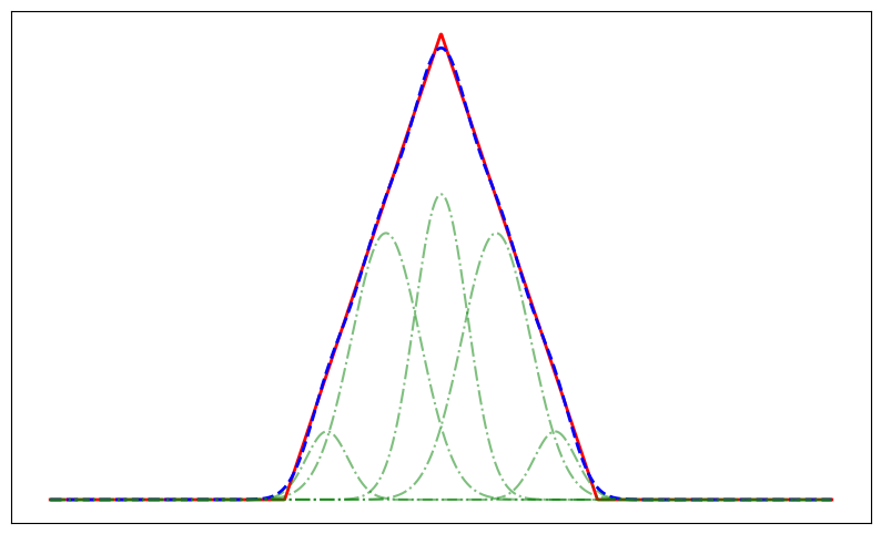
(a) Gaussian ($N=5$)

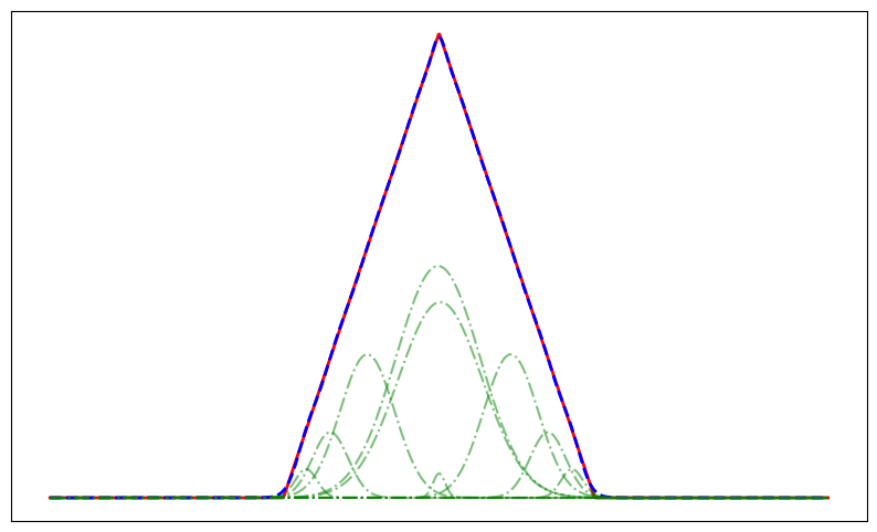
(b) Gaussian ($N=10$)

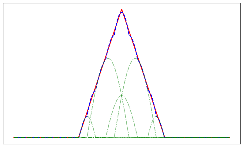
(c) Half-Cosine ($N=5$)

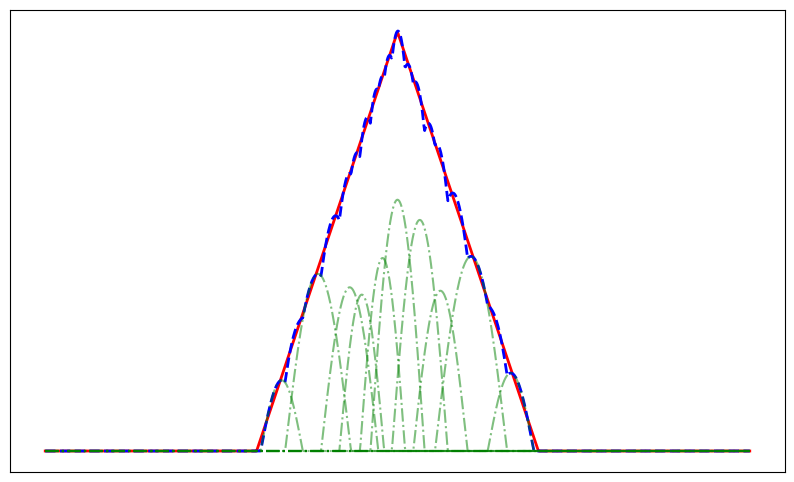
(d) Half-Cosine ($N=10$)

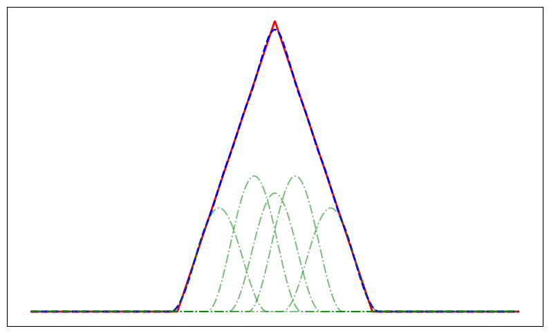
(e) Raised Cosine ($N=5$)

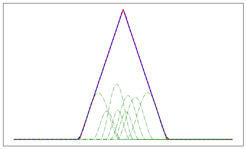
(f) Raised Cosine ($N=8$)

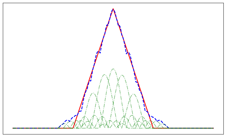
(g) Sinc ($N=9$)

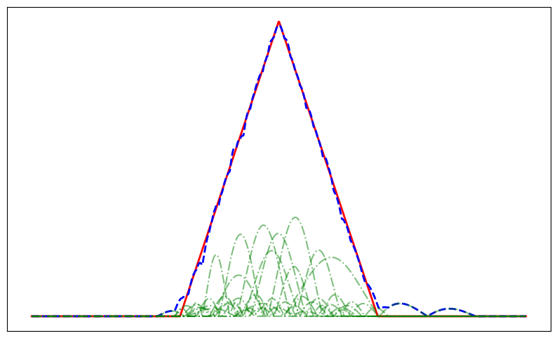
(h) Sinc ($N=10$)

Figure 3: Examples of signal reconstruction through backpropagation using various RBFs. Here the target, reconstructed and individual components are represented by red, blue and green plots, respectively. We achieve competitive results in convergence speed and computational cost. Our raised cosine kernels, for example, achieve convergence faster with fewer components ($N=8$) and at a lower cost of 0.00004 compared to Gaussian kernels, which converge slightly slower at $N=10$ with a comparable cost of 0.0001 in terms of mean squared error.

This pipeline optimizes the number of primitives needed for signal approximation across different reconstruction kernels. Our approach focuses on three key parameters: position, covariance (for signal spread), and amplitude (for signal strength). The model configurations comprises a mixture network of Gaussian, half-cosine, raised-cosine, and modular sinc components, each with a predefined variable number of components. For an extensive analysis of RBFs functions, refer our Supplementary Material.

The model was trained for a fixed number of epochs with respect to a mean squared error loss function, which minimized reconstruction error between the predicted and target signals. Unlike the original Gaussian Splatting algorithm [20], which calculates loss in the projected 2D image space with reconstruction in 3D space, we simplified by calculating the loss and performing the reconstruction directly in 1D because, 1D signal projection cannot be represented in 0D, as this would be meaningless. Finally, a parameter sweep was conducted to identify the optimal configuration with the lowest recorded loss, indicating the optimal number of components.

Table 1: Comparison of simulation results with Gaussian components vs. other reconstruction kernel components. Note that ^∗ indicates that we achieved better reconstruction with fewer components ($N=8$) in terms of mean squared error, using our modified raised cosine pulses compared to Gaussians.

Function	Loss ($N=5$)	Loss ($N=10$)
Gaussian	0.0002	0.0001
Modified half cosine	0.0014	0.0003
Modified raised cosine	0.0002	0.00004∗
Modified sinc (modulus)	0.0030	0.0002

The simulation results indicate that, like Gaussian functions, certain RBFs, can perform comparably or even outperform Gaussians in specific cases. Notably, raised cosines achieved lower reconstruction loss than Gaussians while requiring fewer primitives. These preliminary findings suggest promising alternatives to Gaussian functions and motivate further exploration of these RBFs. Building on this insight, we aim to incorporate these alternative functions into the Gaussian Splatting algorithm, introducing minor adjustments in domain constraints and backpropagation.

4 Method

Next, we will elaborate on the use of DARBFs for 3D reconstruction tasks. We present DARBFs as a plug-and-play replacement for existing Gaussian kernels, offering improvements in aspects such as training time and memory efficiency. The pipeline for DARB splatting is presented in Fig. 4.

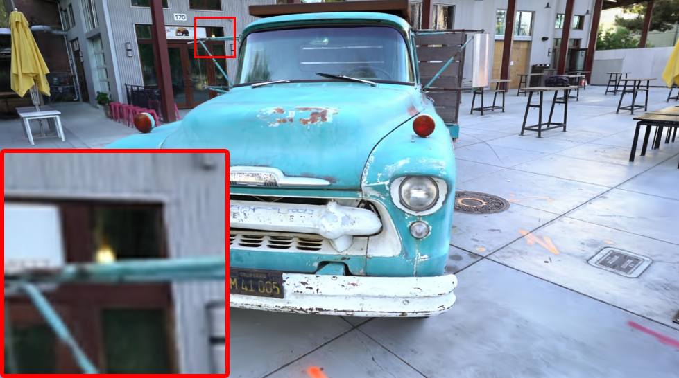
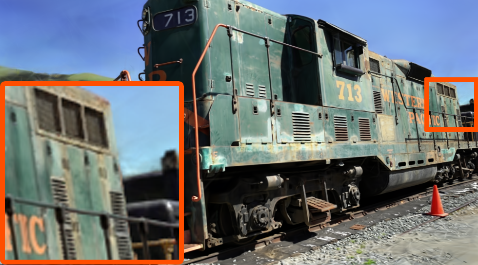
Figure 4: Block diagram: We use the standard optimization pipeline from 3DGS [20] with modifications, introducing a correction factor ($\psi$) to obtain the projected 2D covariance matrix ($\Sigma^{\prime}_{2\times 2}$) compatible with splatting for DARBFs within the existing framework. Our changes within the pipeline are highlighted in red text.

Splatting-based reconstruction methods such as 3DGS [20] obtain the 3D representation of a scene by placing anisotropic Gaussian kernels at 3D points proposed by a SfM pipeline such as COLMAP [45]. The 3DGS Gaussian kernel gets transformed onto the camera frame and projected to the corresponding 2D plane of existing views, resulting in splats. The error between the pixels of these views and blended (rasterized) splats generates the backpropagation signal to optimize the parameters of the 3D Gaussians. The four properties that drive this pipeline are 1. the differentiability of this rasterization, 2. the anisotropic nature of the 3D kernel function (hence the anisotropic nature of the splats), 3. easy projectability, and 4. rapid decay. As seen in [25], the reconstruction kernel function being a function of the Mahalanobis distance $d_{M}$ (Eq. 1), yields the first two properties. A class of functions that display the four properties is non-negative decaying anisotropic radial basis functions (DARBFs) that are functions of Mahalanobis distance [4] $d_{M}$ (Eq. 1). In Sec. 4.1 we propose a method to approximate the projection of DARBFs, thereby satisfying the third property.

4.1 DARB-Splatting

DARB Representation. Similar to 3DGS, we use the same parameterization to represent 3D DARBFs, as the Gaussian function is an instance of the DARBF class. In Table 2, we show the generic mathematical expressions of these reconstruction kernel functions, and Fig. 2 shows their 1D plots. Only some members of the class are shown here, while a broader view is provided in the Supplementary Material. Similar to the Gaussian, most of the chosen DARBFs are strictly decaying, meaning their envelopes decay, which makes them suitable as energy functions. The envelope of the $\mathrm{sinc}$ function, for instance, decays (square-integrable, hence an energy function). To optimize performance, we restricted the spread of most functions to a single pulse (central lobe), ensuring finite support along the reconstruction axes. However, we also observed that comparable results can be achieved with two or more pulses, albeit with a slight trade-off in visual quality (refer Supplementary Material).

Table 2: Overview of decaying anisotropic radial basis functions (DARBFs) in 3D, with essential limits to consider for bounded function applications in 3D reconstruction. Incorporating these limits on Mahalanobis distance $d_{M}$ (defined in Eq. 1) ensures precise control over the main lobe of each function and influence, similar to the 3D Gaussian, for capturing localized features in complex 3D surfaces. Here, the scaling factor $\xi(>0)$ controls the spread of the covariance while $\beta$ decides the roll-off of the main lobe of each DARBF.

Function	Expression	Domain
Modified Gaussian	$\exp\left(-\frac{1}{\xi}\left(d_{M}\right)^{\beta}\right)$	$d_{M}\geq 0$
Modified half cosine	$\cos\left(\frac{1}{\xi}\left(d_{M}\right)^{\beta}\right)$	$\frac{1}{\xi}\left(d_{M}\right)^{\beta}\leq\frac{\pi}{2}$
Modified raised cosine	$0.5+0.5\cdot\cos\left(\frac{1}{\xi}\left(d_{M}\right)^{\beta}\right)$	$\frac{1}{\xi}\left(d_{M}\right)^{\beta}\leq{n\pi}$
Modified sinc (modulus)	$\dfrac{\left|\sin\left(\frac{1}{\xi}\left(d_{M}\right)^{\beta}\right)\right|}{\frac{1}{\xi}\left(d_{M}\right)^{\beta}}$	$\frac{1}{\xi}\left(d_{M}\right)^{\beta}\leq\frac{(n+1)\pi}{2}$
Inv. multi-quadratic	$\dfrac{1}{\left[\frac{1}{\xi}\left(d_{M}\right)^{2}+1\right]^{\frac{1}{2}}}$	$d_{M}\geq 0$

DARB Projection. To project 3D DARBs to DARB-splats, we use the method proposed by EWA Splatting [73, 65]. To project 3D mean ($\mu$) in world coordinate system onto the 2D image plane, we use the conventional perspective projection. However, the same projection cannot be used to project the 3D covariance ($\Sigma$) in world coordinates to the 2D covariance ($\Sigma^{\prime}_{2\times 2}$) in image space. Hence, first, the 3D covariance ($\Sigma$) is projected onto camera coordinate frame which results in a projected $3\times 3$ covariance matrix ($\Sigma^{\prime}$). Given a viewing transformation $W$, the projected covariance matrix $\Sigma^{\prime}$ in camera coordinate frame can be obtained as follows:

$$\Sigma^{\prime}=JW\Sigma W^{T}J^{T}$$ (2)

where $J$ denotes the Jacobian of the affine approximation of the projective transformation. Importantly, integrating a normalized 3D Gaussian along one coordinate axis results in a normalized 2D Gaussian itself. From that, the EWA Splatting [73] shows that the 2D covariance matrix ($\Sigma^{\prime}_{2\times 2}$) of the 2D Gaussian can be easily obtained by taking the sub-matrix of the 3D covariance matrix ($\Sigma^{\prime}$), specifically by skipping the third row and third column (Eq. 4).

However, this sub-matrix shortcut applies only to Gaussian reconstruction kernels due to their inherent properties. Our core argument questions whether the integration described above is essential for the splatting process. While the Gaussian’s closed form integration is convenient, we propose interpreting the 3D covariance as a parameter that represents the 2D covariances from all viewing directions. When viewing a 3D Gaussian from a particular direction, we may think that the opacity would be distributed across the volume defined by each 3D Gaussian, and that alpha blending composites these overlapping volumes. In practice, however, the opacity distribution takes place after projecting 3D Gaussians to 2D splats. Thus, when a ray approaches, it only considers the Gaussian value derived from the 2D covariance of the splat.

As a simple example, consider two 3D Gaussians that are nearly identical in all properties except for the variance along the z-axis ($(\sigma^{\prime}_{z})^{2}$). When these two Gaussians are projected into 2D, we expect the 3D Gaussian with a higher $\sigma^{\prime}_{z}$ to have greater opacity values. In contrast, 3DGS yields a similar matrix ($\Sigma^{\prime}_{2\times 2}$) for both covariances, while exerting the same influence on opacity distribution along the splats. This further strengthens our argument for treating $\Sigma^{\prime}$ as a parameter to represent $\Sigma^{\prime}_{2\times 2}$.

Generally, for DARBFs, integrating a 3D DARB along a certain axis does not yield the same DARBF in 2D, nor does it result in a closed-form solution. Therefore, we established the relationship between $\Sigma^{\prime}$ and $\Sigma^{\prime}_{2\times 2}$ for DARBFs through simulations. For clarity, we briefly provide the derivations for the half-cosine squared splat here, whereas detailed derivations and corresponding CUDA script modifications for all DARBFs are provided in the Supplementary Material. The 3D half-cosine squared kernels is as follows:

$$P_{i,j,k}=\begin{cases}\cos\left(\frac{\pi}{18}(d_{M})^{2}\right),&\text{if }\ (d_{M})^{2}<9,\\ 0,&\hfill\text{otherwise}.\end{cases}$$ (3)

where $d_{M}$ (Eq. 1) is the Mahalanobis distance. We then calculate the projected $\Sigma^{\prime}_{2\times 2}$ by summing values along a certain axis, similar to integrating along the same axis. Through experimentation with various values, we determined that the estimated $\Sigma^{\prime}_{2\times 2}$ 2D covariance matrix is also symmetric, due to the strict decomposition of the 3D covariance matrix to maintain a positive definite matrix, independent of the third row and column of $\Sigma^{\prime}$. Additionally, we obtain $\Sigma^{\prime}_{2\times 2}$ by multiplying $\Sigma^{\prime}$ with a correction factor $\psi$ (Eq. 4), which we estimate separately for each reconstruction kernel using Monte Carlo experiments. For half-cosine squares we estimated $\psi=1.36$.

$$\Sigma^{\prime}=\begin{pmatrix}a&b&c\\ b&d&e\\ e&d&f\\ \end{pmatrix}\rightarrow\psi\begin{pmatrix}a&b\\ b&d\\ \end{pmatrix}=\Sigma^{\prime}_{2\times 2}.$$ (4)

Similarly, based on such empirical results, we modified the existing CUDA scripts of 3DGS [20] to implement each DARBF separately with its respective $\psi$ value to ensure comparable results. Additionally, we introduce a scaling factor $\xi$ to match the extent of our function closely with the Gaussian, allowing a fair comparison of DARBF performance. Although Gaussian functions are spatially infinite, 3DGS [20] uses a bounded Gaussian to limit the opacity distribution in 2D, thereby reducing unnecessary processing time. For projected 2D splats, they calculate the maximum radius as $R=3\cdot\sqrt{\max\{\lambda_{1},\lambda_{2}\}}$ , where $\lambda_{1}$ and $\lambda_{2}$ denote the eigenvalues of the 2D covariance matrix $\Sigma^{\prime}_{2\times 2}$. Using this radius $R$, we obtain a similar extent for DARBFs as Gaussians with the help of $\xi$. Taking that into consideration, the 2D half-cosine squared splat is defined as follows:

$$w=\cos\left(\frac{\left(x-\boldsymbol{\mu^{\prime}}\right)^{T}\boldsymbol{(}\Sigma^{\prime}_{2\times 2})^{-1}\left(x-\boldsymbol{\mu^{\prime}}\right)}{\xi}\right),$$ (5)

where $x\in\mathbb{R}^{2}$ is the position vector, $\mu^{\prime}\in\mathbb{R}^{2}$ is the projected mean, and $\Sigma^{\prime}_{2\times 2}\in\mathbb{R}^{2\times 2}$ represents the covariance matrix. Here, $R_{\text{cosine}}$ will be $\frac{\sqrt{2\pi\xi\max(\lambda_{1},\lambda_{2})}}{2},$ indicating 100% extent, as we consider the entire central lobe. However, for a 2D Gaussian with an extent of 99.7% (up to three standard deviations), the radius $R_{\text{Gaussian}}$ is given by $3\sqrt{\max(\lambda_{1},\lambda_{2})}.$ To match the extent of both functions, we select $\xi(>0)$ such that $\frac{\sqrt{2\pi\xi\max(\lambda_{1},\lambda_{2})}}{2}=3\sqrt{\max(\lambda_{1},\lambda_{2})}$, which implies $\xi=\frac{18}{\pi}$.

Within this bounded region, we use our footprint function (Eq. 21) to model the opacity, similar to the approach in 3DGS. Following this, we apply alpha blending to determine the composite opacity [20, 65] for each pixel, eventually contributing to the final color of the 2D rendered image.

Ground Truth

Raised cosines (Ours)

3DGS

Half-cosine Squares (Ours)

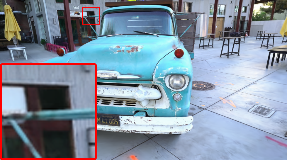
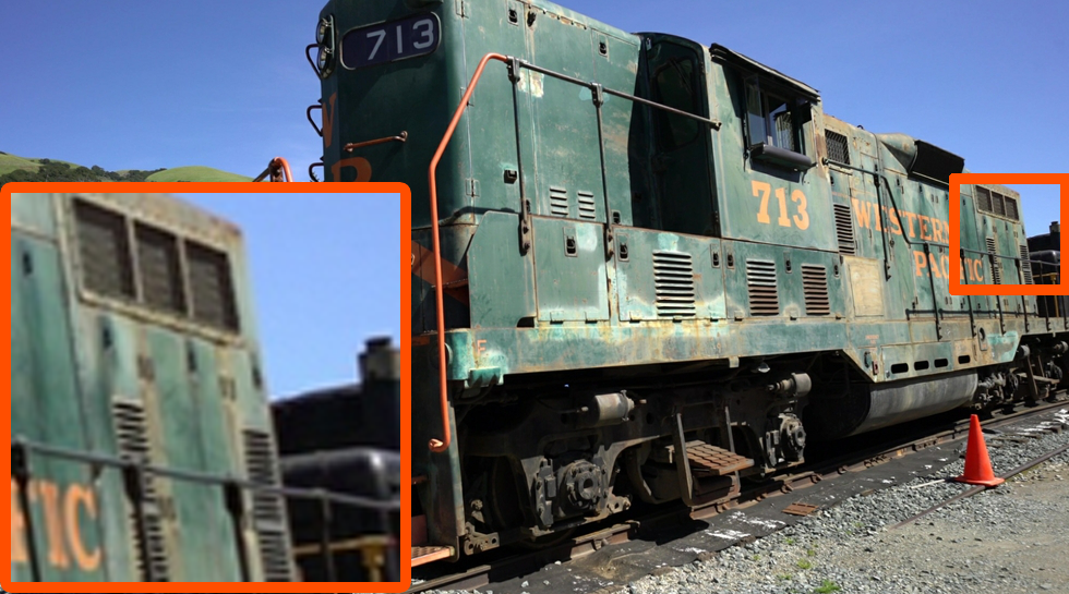
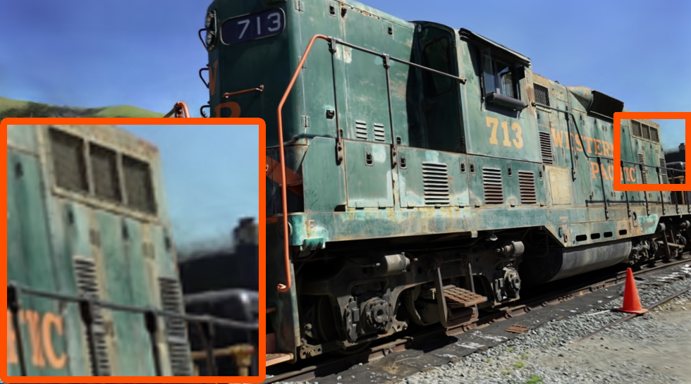
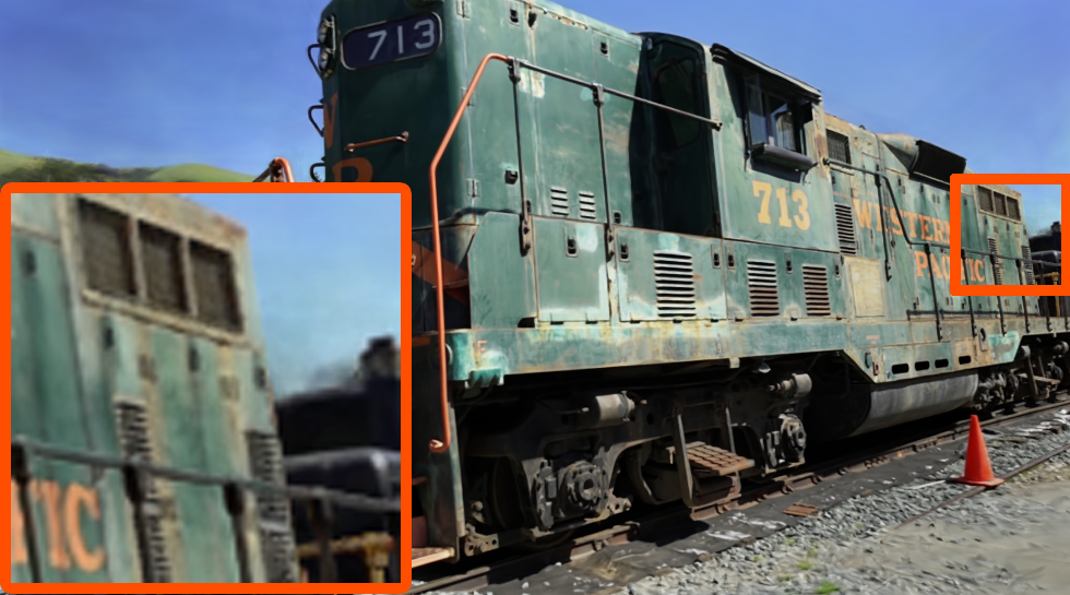
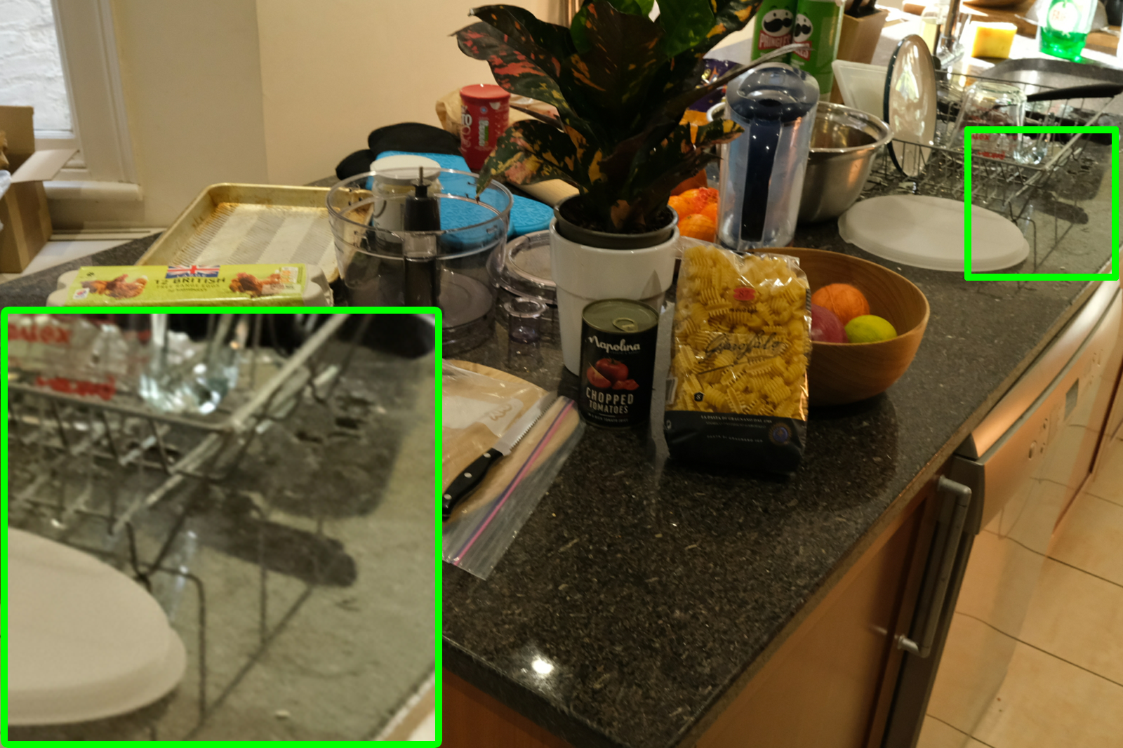
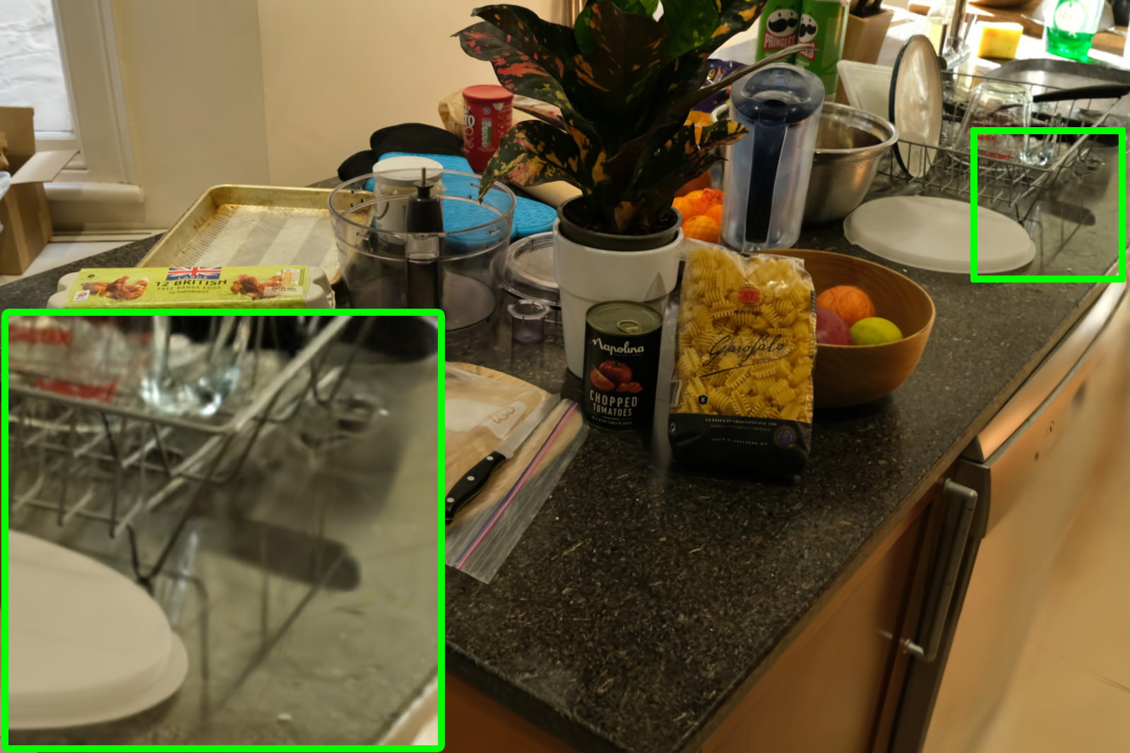
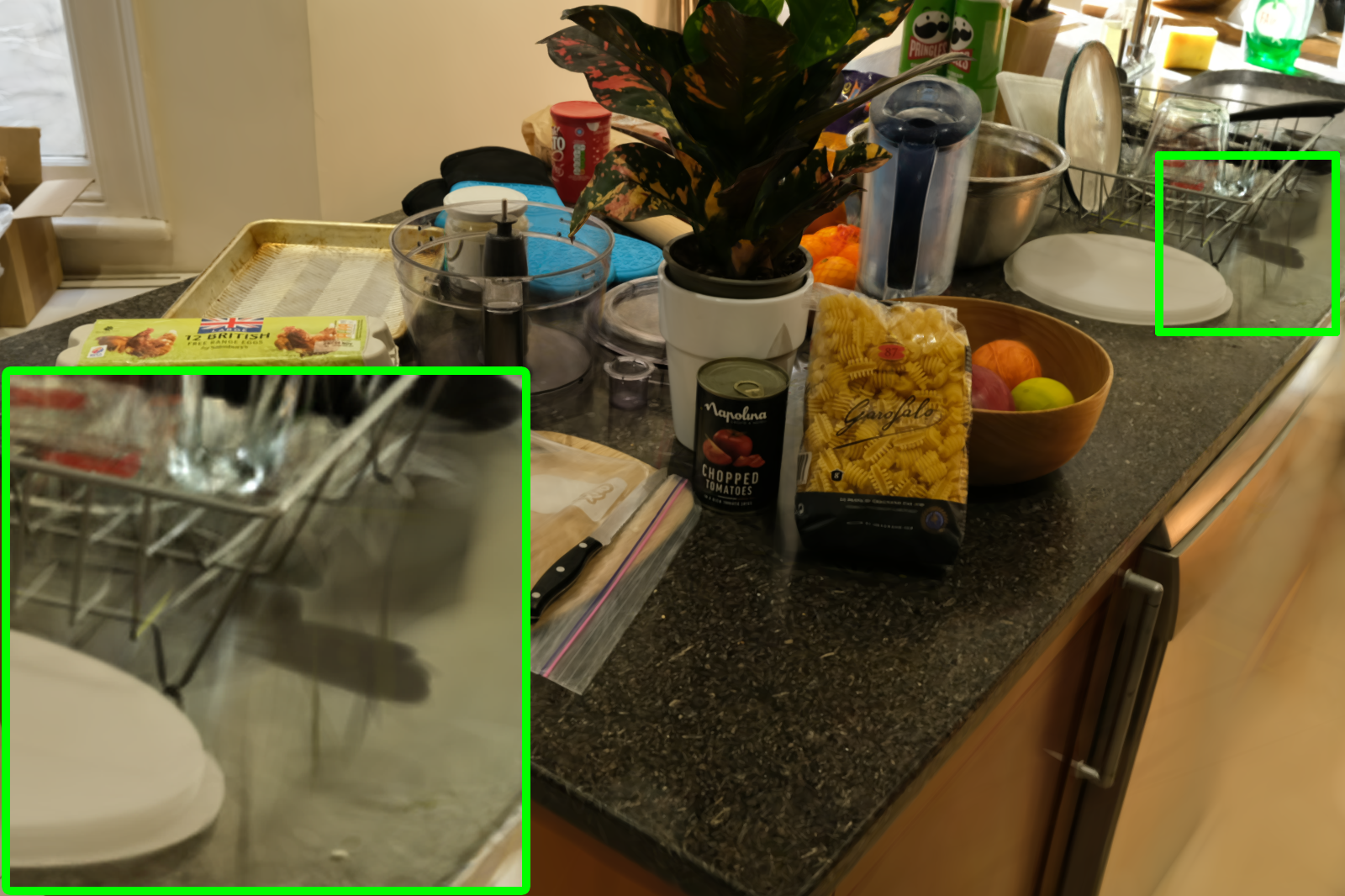
Figure 5: Visual comparison on NVS. We present comparisons between our proposed methods (Raised cosine and half-cosine squares) and established baseline (3DGS) alongside their respective ground truth images. The displayed scenes are ordered as follows: TRUCK and TRAIN from Tanks&Temples [22] dataset; COUNTER from Mip-NeRF360 [2] dataset. We highlight subtle improvements in our approach, such as the appearance of a light bulb in the rendered image of the first row, which is absent in the splitting algorithm. Additionally, the edges of the train and the shadows of the rack in the images on the second and third rows, respectively, are noticeably sharper, whereas these details appear blurred in the original splitting algorithm. Note that in addition to improved reconstruction, we also achieve significantly better training and memory efficiency with these alternative primitives (see Table 3).

4.2 Backpropagation and Error Calculation

To support backpropagation, we must account for the differentiability of DARBFs. As usual, the backpropagation process begins with a loss function that combines the same losses discussed in the original work [20]: an $\mathcal{L}_{1}$ loss and an SSIM (Structural Similarity Index Measure) loss, which guide the 3D DARBs to optimize its parameters.

$$\mathcal{L}=(1-\lambda)\mathcal{L}_{1}+\lambda\mathcal{L}_{\text{D-SSIM}}$$ (6)

where $\lambda$ denotes each loss term’s contribution to the final image loss. After computing the loss, we perform backpropagation, where we explicitly modify the differentiable Gaussian rasterizer from 3DGS [20] to support respective gradient terms for each DARBF. The following example demonstrates these modifications for the 3D half-cosine squared function (Eq. 21) with $\xi=\frac{18}{\pi}\$.

$$\footnotesize\frac{dw}{d(x-\boldsymbol{\mu^{\prime}})}=\frac{-2\,(\Sigma^{\prime}_{2\times 2})^{-1}\,(x-\mu^{\prime})\,\sin\left(\frac{\left(x-\boldsymbol{\mu^{\prime}}\right)^{T}(\Sigma^{\prime}_{2\times 2})^{-1}\left(x-\boldsymbol{\mu^{\prime}}\right)}{\xi}\right)}{\xi}$$ (7)

$$\footnotesize\frac{dw}{d((\Sigma^{\prime}_{2\times 2})^{-1})}=\frac{-(x-\mu^{\prime})\,\left(x-\boldsymbol{\mu^{\prime}}\right)^{T}\,\sin\left(\frac{\left(x-\boldsymbol{\mu^{\prime}}\right)^{T}(\Sigma^{\prime}_{2\times 2})^{-1}\left(x-\boldsymbol{\mu^{\prime}}\right)}{\xi}\right)}{\xi}$$ (8)

Function	Mip-NeRF360					Tanks & Temples					Deep Blending
	SSIM$\uparrow$	PSNR$\uparrow$	LPIPS$\downarrow$	Train	Memory	SSIM$\uparrow$	PSNR$\uparrow$	LPIPS$\downarrow$	Train	Memory	SSIM$\uparrow$	PSNR$\uparrow$	LPIPS$\downarrow$	Train	Memory
3DGS (7k) [20]	0.770	25.60	0.279	4m 43s∗	523 MB	0.767	21.20	0.28	5m 05s∗	270 MB	0.875	27.78	0.317	3m 22s∗	368 MB
3DGS (30K) [20]	0.815	27.21	0.214	30m 33s∗	734 MB	0.841	23.14	0.183	19m 46s∗	411 MB	0.903	29.41	0.243	26m 29s∗	676 MB
GES [15]	0.794	26.91	0.250	23m 31s∗	377 MB	0.836	23.35	0.198	15m 26s∗	222 MB	0.901	29.68	0.252	22m 44s∗	399 MB
3DGS-updated (7K)	0.769	25.95	0.281	3m 24s	504 MB	0.781	21.78	0.261	2m 02s	293 MB	0.879	28.42	0.305	3m 14s	462 MB
3DGS-updated (30K)	0.813	27.45	0.218	19m 06s	633 MB	0.847	23.77	0.173	11m 24s	371 MB	0.901	29.66	0.242	20m 12s	742 MB
Raised cosine (7K)	0.773	26.01	0.273	3m 13s	513 MB	0.788	21.88	0.251	1m 59s	304 MB	0.882	28.47	0.300	2m 57s	401 MB
Raised cosine (30K)	0.813	27.45	0.214	19m 36s	645 MB	0.851	23.64	0.166	12m 06s	364 MB	0.901	29.63	0.240	20m 01s	767 MB
Half cosine (7K)	0.737	25.46	0.316	2m 52s	400 MB	0.749	21.071	0.295	1m 42s	244 MB	0.872	27.938	0.320	2m 42s	355 MB
Half cosine (30K)	0.790	27.04	0.247	16m 15s	524 MB	0.824	23.108	0.201	9m 11s	338 MB	0.900	29.38	0.253	17m 35s	634 MB
Modular Sinc (7K)	0.751	25.74	0.302	3m 20s	439 MB	0.767	21.59	0.276	2m 04s	255 MB	0.878	28.39	0.308	3m 17s	399 MB
Modular Sinc (30K)	0.801	27.30	0.234	18m 50s	622 MB	0.836	23.51	0.189	16m 08s	333 MB	0.901	29.66	0.247	20m 47s	682 MB

Table 3: Splatting results: The best values are highlighted in red and second-best values in orange, the third-best values in light orange, and the fourth-best in yellow. Note that, ^∗ denotes the difference in computation power that is used to implement our model and previous models (3DGS [20], GES [15]), hence we used a speed-up factor (see Supplementary Materials), to get fair results regarding training time which is available in the original publication. Our DARBFs were implemented based on the updated 3DGS codebase. Our DARB splatting with raised cosine function was able to achieve on-par performance regarding PSNR, SSIM, LPIPS and training duration. Also, half cosine square shows a significant reduction in training time. We evaluate the performance of each model by considering the results at 7K and 30K iteration checkpoints.

5 Experiments

Experimental Settings. We anchor our contributions on the recently updated codebase of 3DGS [20], adjusting the CUDA scripts to support a range of DARBFs. For a fair comparison, we use the same testing scenes as the 3DGS paper, including both bounded indoor and large outdoor environment scenes from various datasets [2, 22, 17]. We utilized the same COLMAP [45] initialization provided by the official dataset for all tests conducted to ensure fairness. Furthermore, we retained the original hyperparameters, adjusting only the opacity learning rate to 0.02 for improved results. All experiments and evaluations were conducted, and further verified on a single NVIDIA GeForce RTX 4090 GPU.

We compare our work with SOTA splatting-based methods that use exponential family reconstruction kernels, such as the original 3DGS, updated codebase of 3DGS, and GES [15] as benchmarks. We also evaluated the DARBFs using the standard and frequently used PSNR, LPIPS and SSIM metrics similar to these benchmarks (Table 3).

5.1 Results

Table 4: Comparison of various 3D reconstruction methods, showing that our approach outperforms prior methods in PSNR, LPIPS, and training efficiency metrics. Note that the benchmark values for 3DGS and GES are sourced directly from their respective papers, and therefore may not represent an entirely fair comparison.

Method	SSIM$\uparrow$	PSNR$\uparrow$	LPIPS$\downarrow$	Train$\downarrow$
Plenoxels [12]	0.626	23.08	0.463	19m∗
INGP [36]	0.699	25.59	0.331	5.5m∗
Mip-NeRF360 [2]	0.792	27.69	0.237	48h
3DGS [20]	0.815	27.21	0.214	30m∗
GES [15]	0.794	26.91	0.250	23m∗
DARBS (RC)	0.813	27.45	0.214	19min
DARBS (HC)	0.790	27.04	0.247	16min

Table 3 summarizes the comparative analysis across various datasets alongside our benchmarks. It shows that different functions perform better quantitatively in various aspects, such as training time, memory efficiency, and visual quality. Results show that the modified raised cosine function with $\xi=\frac{2.5}{\pi}\$ achieves on-par results in terms of PSNR, LPIPS and SSIM metrics with the SOTA original and updated codebase of 3DGS [20], further validating our 1D simulation results discussed in Sec. 3.2. Additionally, it demonstrates that certain DARBFs, despite not belonging to the exponential family, are able to compete effectively with our previous related work benchmark [15].

Half-cosine squares with $\xi=\frac{18}{\pi},\$ achieve approximately a 15%  reduction in training time compared to Gaussians (updated codebase) on average across all scenes, with a notably modest trade-off in visual quality of less than 0.5 dB on average. This is because a half-cosine square spans a larger region compared to a Gaussian. With precomputed scaling factors for each DARBF, there is no additional computational overhead in the rendering pipeline, resulting in comparable rendering times to Gaussians. Fig. 5 shows that raised cosine captures fine details better than Gaussians, and Table 4 presents a comparative analysis of our method across various 3D reconstruction methods.

5.2 Ablation Study

Decaying ARBFs. We validated various reconstruction kernels through low-dimensional simulations (Sec. 3.2), showing that normalized, decaying functions focus energy near the origin (Sec. 4.1), ensuring each sample’s influence on the reconstruction is strongest its point, aiding accurate signal reconstruction. In contrast, the instability caused by unbounded growing functions led to their omission in favor of DARBFs.

Correction factor. The existing pipeline was built upon the prominent property of Gaussians, where integrating along a specific axis results in the same function, in a lower dimension. However, DARBFs generally do not exhibit this property. To incorporate DARBFs into the original pipeline, we introduced a correction factor $\psi$ to approximate the projected covariance (Sec. 4.1). As shown in Table 5, this modification significantly enhanced the performance of DARBFs, achieving comparable results across all scenes in the Mip-NeRF 360 dataset on average for raised cosines, relative to the updated 3DGS codebase, implying outperformance of the same in the original 3DGS results.

Table 5: Comparison of PSNR, SSIM, and LPIPS metrics for Mip-NeRF 360 scenes under the influence of $\psi$.We claim that incorporating $\psi$ not only enhances the performance of our kernels but also serves as the pivotal factor in surpassing the 3DGS results.

	with $\psi$			without $\psi$
Scenes	PSNR	SSIM	LPIPS	PSNR	SSIM	LPIPS
3DGS-updated	—	—	—	27.45	0.81	0.22
Raised Cosine	27.45	0.81	0.21	26.69	0.78	0.25
Half Cosine	27.04	0.79	0.25	25.89	0.76	0.28

6 Conclusion and Discussion

To the best of our knowledge, we are the first to generalize splatting techniques with DARB-Splatting, extending beyond the conventional exponential family. In introducing this new class of functions, DARBFs, we highlight the distinct performances of each function. We establish the relationships between 3D covariance and 2D projected covariance through Monte Carlo experiments, providing an effective approach for understanding covariance transformations under projection. Our modified CUDA codes for each DARBF are available to facilitate further research and exploration in this area.

Limitation. While we push the boundaries of splatting functions with DARBFs, the useful properties and capabilities of each function for 3D reconstruction, within a classified mathematical framework, remain to be fully explored. Future research could explore utility applications and the incorporation of existing signal reconstruction algorithms, such as the Gram-Schmidt process, with DARBFs.

Supplementary Material

7 DARB-Splatting

We generalize the reconstruction kernel to include non-exponential functions by introducing a broader class of Decaying Anisotropic Radial Basis Functions (DARBFs). One of the main reasons why non-exponential functions have not been widely explored is the advantageous integration property of the Gaussian function, which simplifies the computation of the 2D covariance of a splat. However, through Monte Carlo experiments, we demonstrate that DARBFs can also exhibit this desirable property, even though most of them lack a closed-form solution for integration. Additionally, the integration of DARBFs does not generally relate to other DARBFs.

We also explained (Sec. 4.1), using an example, that in 3DGS [20], the opacity contribution for each pixel from a reconstruction kernel (3D) is derived from its splats (2D), rather than from their 3D volume. Based on this, we consider the covariance in 3D as a variable representing the 2D covariances in all directions. In the next section, we describe the Monte Carlo experiments we conducted, supported by mathematical equations.

In surface reconstruction tasks [5], DARBFs leverage principal component analysis (PCA) of the local covariance matrix to identify directionally dependent features and orient the 3D ellipsoids accordingly. This approach enables DARBFs to model local anisotropies in the data and reconstruct surfaces, preserving fine details more effectively than isotropic models. Furthermore, the decaying nature of these functions, as presented in Table 2, results in a more localized influence, effectively focusing the function within a certain radius. This localization is advantageous in 3D reconstruction, where only neighboring points contribute significantly to a given point in space, ensuring smooth blending. Therefore, we can conclude that all DARBFs are suitable for splatting. Although there are many DARBFs, we focus on a selected few here due to limited space. In the following sections, we elaborate on the mathematical formulation of these selected DARBFs, outline their computational implementation, and demonstrate their utility in accurately modeling complex opacity distributions in the context of 3D scene reconstruction.

7.1 Mathematical Expressions of Monte Carlo Experiments

When it comes to 3DGS [20], we initially start with a $3\times 3$ covariance matrix in the 3D world coordinate system. By using,

$$\Sigma^{\prime}=JW\Sigma W^{T}J^{T}$$ (9)

we obtain a $3\times 3$ covariance matrix ($\Sigma^{\prime}$) in the camera coordinate space. According to the integration property mentioned in the EWA Spatting paper [73], this $\Sigma^{\prime}$ can be projected into a $2\times 2$ covariance matrix in the image space ($\Sigma^{\prime}_{2\times 2}$) by simply removing the third row and column of $\Sigma^{\prime}$. However, the same process does not apply to other DARBFs. For instance, there is no closed-form solution for the marginal integration of the half-cosine and raised-cosine functions used in this paper. To simplify the understanding of this integration process and address this issue, we conducted the following experiment.

Experimental Setup. First, we introduce our 3D point space with $x,y,z$ coordinates in equally spaced intervals for $N$ number of points, a random mean vector ($\mu$) and a random $3\times 3$ covariance matrix ($\Sigma$). Based on a predetermined limit specific for each DARBF (we will discuss about this in Sec. 7.2), we calculate the density/power assigned by the DARB kernel at a particular point $\boldsymbol{x}$ in 3D space as follows:

$$P=\cos\left(\frac{2\pi\left(\boldsymbol{x}-\boldsymbol{\mu}\right)^{T}\boldsymbol{(}\Sigma)^{-1}\left(\boldsymbol{x}-\boldsymbol{\mu}\right)}{36}\right),$$ (10)

where $\boldsymbol{x}=\begin{bmatrix}x_{i}&y_{i}&z_{i}\end{bmatrix}$. As for the integration, we take the sum of these $P$ ($P\in\mathbb{R}^{N\times N\times N}$) matrices along one dimension (for instance, along $z$ axis) and name it $total\_density$, which can be obtained as follows:

$$\text{total\_density}\,(x,y)=\sum_{z}P(x,y,z)$$ (11)

where $total\_density\in\mathbb{R}^{N\times N}$. This will, for example, integrate the cosine kernel in Eq. 10 along $z$-direction, collapsing into a 2D density in XY plane. Following this integration, these total densities will be normalized as follows:

$$\text{total\_density}_{\text{normalized}}=\frac{\text{total\_density}}{\max(\text{total\_density})}$$ (12)

This normalization step does not change the typical covariance relationship. To compare with other functions’ projection better, we use this normalization, so that the maximum of total density will be equal one.

For the visualization of these 2D densities, we create a 2D mesh grid by using only $x,y$ coordinate matrices called $coords\in\mathbb{R}^{N^{2}\times 2}$. At the same time, we flatten the 2D density matrix and get a density grid as $density\in\mathbb{R}^{N^{2}\times 1}$.

If the dimensions of $x,y$ coordinates are different, we need to repeat the $coords$ and $density$ arrays separately to perfectly align each 2D coordinate for its corresponding density value. Since we use the same dimension for $x,y$ coordinates, we can skip this step. By using these $coords$ and $density$ matrices, we then calculate the weighted covariance matrix as follows:

$$\begin{array}[]{cc}\bar{x}=\frac{\sum_{i=1}^{N^{\prime}}w_{i}x_{i}}{\sum_{i=1}^{N^{\prime}}w_{i}}&\bar{y}=\frac{\sum_{i=1}^{N^{\prime}}w_{i}y_{i}}{\sum_{i=1}^{N^{\prime}}w_{i}}\end{array}$$

where $N^{\prime}=N^{2}$ and $w_{i}$ denote the corresponding parameters from the $density$ matrix. Finally, the vector $\bar{\boldsymbol{m}}$ is given by:

$$\bar{\boldsymbol{m}}=\begin{bmatrix}\bar{x}\\ \bar{y}\end{bmatrix}_{2\times 1}$$ (13)

By using the above results, we can determine the projected $2\times 2$ covariance matrix ($\Sigma^{\prime}_{2\times 2}$) as follows:

$$\Sigma^{\prime}_{2\times 2}=\begin{bmatrix}\sigma_{xx}&\sigma_{xy}\\ \sigma_{xy}&\sigma_{yy}\end{bmatrix}$$

where $\sigma_{xx}$, $\sigma_{yy}$ and $\sigma_{xy}$ terms can be determined as:

$$\sigma_{xx} =\frac{\sum_{i=1}^{N}w_{i}(x_{i}-\bar{x})^{2}}{\sum_{i=1}^{N}w_{i}}\qquad \sigma_{yy} =\frac{\sum_{i=1}^{N}w_{i}(y_{i}-\bar{y})^{2}}{\sum_{i=1}^{N}w_{i}}$$

$$\sigma_{xy} =\frac{\sum_{i=1}^{N}w_{i}(x_{i}-\bar{x})(y_{i}-\bar{y})}{\sum_{i=1}^{N}w_{i}}$$

We can express this entire operation in matrix form as follows:

$$\Sigma^{\prime}_{2\times 2}=\frac{1}{\sum_{i=1}^{N^{\prime}}w_{i}}\sum_{i=1}^{N^{\prime}}w_{i}\left(\boldsymbol{x}_{i}-\bar{\boldsymbol{m}}\right)\left(\boldsymbol{x}_{i}-\bar{\boldsymbol{m}}\right)^{T}$$ (14)

$$\text{where}\quad\boldsymbol{x}_{i}=\begin{bmatrix}x_{i}\\ y_{i}\end{bmatrix}$$

Based on this simulation, we received the projected $2\times 2$ covariance matrix ($\Sigma^{\prime}_{2\times 2}$) for different DARBFs and identified that they are not integrable for volume rendering [73]. Simply saying, we cannot directly obtain the first two rows and columns of $\Sigma^{\prime}_{2\times 2}$ from the first two rows and first tow columns of the 3D covariance matrix $\Sigma^{\prime}_{3\times 3}$ as they are. But we noticed that there is a common ratio between the values of these two matrices. To resolve this issue, we introduce a correction factor $\psi$ as a scalar to multiply with the $\Sigma^{\prime}_{2\times 2}$ matrix. This scalar holds different values for different DARBFs since their density kernels act differently.

7.2 Determining the Boundaries of DARBFs

From the 1D signal reconstruction simulations (Sec. 3.2 and Sec.  10) and the splatting results (Sec.  10), we demonstrate that strictly decaying functions can represent the scenes better. Therefore, we use the limits for each function to ensure the strictly decaying nature, while also considering the size of each splat. By restricting to a single pulse, we achieve a more localized representation, resulting in better quality. Incorporating more pulses allows them to cover a larger region compared to one pulse (with the same $\xi$ and $\beta$), leading to memory reduction, albeit with a tradeoff in quality.

In 3DGS [20], opacity modeling happens after the projection of the 3D covariance ($\Sigma$) in world coordinate space onto 2D covariance ($\Sigma^{\prime}_{2\times 2}$) in image space. By using the inverse covariance ($\Sigma^{\prime-1}_{2\times 2}$) and the difference between the center of the splat ($\mu^{\prime}$) and the coordinates of the selected pixel, they introduce the Mahalnobis component (Eq. 1) within the Gaussian kernel to model the opacity distribution across each splat. When determining the final color of a particular pixel, they have incorporated a bounding box mechanism to identify the area which a splat can have the effect when modeling the opacity, so that they can do the tile-based rasterization using the computational resources efficiently.

Since the Gaussian only has a main lobe, we can simply model the opacity distribution across a splat using the bounding box mentioned in Sec. 4.1. This bounding box, determined by the radius $R=3\cdot\sqrt{\max\{\lambda_{1},\lambda_{2}\}}$, where $\lambda_{1}$ and $\lambda_{2}$ denote the eigenvalues of the 2D covariance matrix $\Sigma^{\prime}_{2\times 2}$ (Sec. 4.1), will cover most of the function (main lobe), affecting the opacity modeling significantly. However, in our DARBFs, we have multiple side lobes which can have an undesirable effect on this bounding box unless the range is specified correctly. If these side lobes are included within the bounding box, each splat will have a ring effect in their opacity distributions.

To avoid this ring effect, we identified the range of the horizontal spread of the main lobe of each DARBF in terms of their Mahalanobis distance component and introduced a limit in opacity distribution to carefully remove the effects from their side lobes. In our Monte Carlo experiments (Sec. 7.1), we used this limit in the 3D DARB kernel, as we directly perform the density calculation in 3D and the projection onto 2D image space afterwards. For example, let us consider the 3D raised cosine as follows:

$$w=0.5+0.5\cos\left(\frac{2\pi d_{M}^{2}}{5}\right)$$ (15)

where $\xi=\frac{5}{2\pi}$ and $\beta=2$ according to the standard expression mentioned in Table 2. To avoid the side lobes and only use the main lobe, we assess the necessary range that we should consider with the Gaussian curves in 1D and chose the following limit (according to Table 2):

$$d_{M}^{2}<6.25=\left(\pi\times\frac{5}{2\pi}\right)^{2}$$ (16)

If the above limit is not satisfied by the Mahalanobis component, the density value will be taken as zero for those cases. As in the Table 2, this limit will be different for different DARBFs since each DARBF shows different characteristics regarding their spread, main lobe and side lobes. Applying these limits will help to consider the 100$\%$ support of the main lobe of each DARBF into the bounding box.

Even though we apply these limits on the 3D representation of each kernel and calculate the densities, in our reconstruction pipeline, we use these limits on DARB splats (2D) similar to 3DGS [20]. In our experiments, our main target was to identify the relationship between the 2D covariance $\Sigma^{\prime}_{2\times 2}$ and the 3D sub-matrix $\Sigma^{\prime}_{3\times 3}$ (Sec. 7.1), and implement these limits on 3D DARB kernels.

8 DARB-Splatting Implementation

Here, we present the reconstruction kernel (3D) and splat (2D) functions (footprint functions) for selected DARBFs, along with their respective derivative term modifications related to backpropagation, in both mathematical expressions and CUDA codes. These modifications have been incorporated into the splatting pipeline and CUDA code changes. In the code, $d$ denotes $x-\boldsymbol{\mu}^{\prime}$ , and $con=\begin{bmatrix}a&b\\ b&c\end{bmatrix}$ denotes the inverse of the 2D covariance matrix $(\Sigma^{\prime}_{2\times 2})^{-1}$ in the mathematical form. For each DARBF, we clearly show $\xi$ and $d_{M}$ in the code. We use a unique correction factor $\psi$ for each DARBF, determined through Monte Carlo experiments, to compute $\Sigma^{\prime}_{2\times 2}$ from $\Sigma^{\prime}$.

8.1 Raised Cosine Splatting

Here, a single pulse of the raised cosine signal is selected for enhanced performance. The 3D raised cosine function is as follows:

$$0.5+0.5\cos\left(\frac{1}{\xi}\left(d_{M}\right)\right),\quad\frac{1}{\xi}\left(d_{M}\right)\leq\pi$$ (17)

The raised cosine splat function is as follows:

$$w=0.5+0.5\cos\left(\frac{\sqrt{\left(x-\boldsymbol{\mu^{\prime}}\right)^{T}\boldsymbol{\Sigma^{\prime}}_{2\times 2}^{-1}\left(x-\boldsymbol{\mu^{\prime}}\right)}}{\xi}\right),$$ (18)

$$\frac{\sqrt{\left(x-\boldsymbol{\mu^{\prime}}\right)^{T}\boldsymbol{\Sigma^{\prime}}_{2\times 2}^{-1}\left(x-\boldsymbol{\mu^{\prime}}\right)}}{\xi}\leq\pi$$

Modifications in derivative terms related to the raised cosine splat during backpropagation are provided next.

$$\frac{\partial w}{\partial(x-\boldsymbol{\mu^{\prime}})}=-\frac{0.5}{\xi}\sin\left(\frac{\sqrt{\left(x-\boldsymbol{\mu^{\prime}}\right)^{T}\boldsymbol{\Sigma^{\prime}}_{2\times 2}^{-1}\left(x-\boldsymbol{\mu^{\prime}}\right)}}{\xi}\right)\cdot\frac{\boldsymbol{\Sigma^{\prime}}_{2\times 2}^{-1}(x-\boldsymbol{\mu^{\prime}})}{\sqrt{\left(x-\boldsymbol{\mu^{\prime}}\right)^{T}\boldsymbol{\Sigma^{\prime}}_{2\times 2}^{-1}\left(x-\boldsymbol{\mu^{\prime}}\right)}}.$$ (19)

$$\frac{\partial w}{\partial\boldsymbol{\Sigma^{\prime}}_{2\times 2}^{-1}}=-\frac{0.5}{\xi}\sin\left(\frac{\sqrt{\left(x-\boldsymbol{\mu^{\prime}}\right)^{T}\boldsymbol{\Sigma^{\prime}}_{2\times 2}^{-1}\left(x-\boldsymbol{\mu^{\prime}}\right)}}{\xi}\right)\cdot\frac{\left(x-\boldsymbol{\mu^{\prime}}\right)\left(x-\boldsymbol{\mu^{\prime}}\right)^{T}}{\sqrt{\left(x-\boldsymbol{\mu^{\prime}}\right)^{T}\boldsymbol{\Sigma^{\prime}}_{2\times 2}^{-1}\left(x-\boldsymbol{\mu^{\prime}}\right)}}.$$ (20)

The following CUDA code modifications were implemented to support raised cosine splatting.

⬇

1float correctionFactor = 0.655f; // The correction factor we introduce

2cov *= correctionFactor ; // Multiply the 3D covariance matrix by the correction factor

3

4float ellipse = con_o.x * d.x * d.x + con_o.z * d.y * d.y + 2.f * con_o.y * d.x * d.y; // dM**2

5if (ellipse < 0 || ellipse > 6.25f) // Limit set on 2D ellipse to restrict to one pulse

6 continue;

7float ellipse_root = sqrt(ellipse); // dM

8float ellipseFactor = M_PI * ellipse_root / 2.5f; // Here scaling factor, xi = 5/(2 * math_pi)

9const float Cosine = 0.5f + .5f * cos(ellipseFactor);

10const float alpha = min(0.99f, con_o.w * Cosine); // w * raised cosine

Listing 1: Modifications in forward propagation in CUDA rasterizer for raised cosine splatting.

⬇

1float correctionFactor = 0.655f;

2cov2D *= correctionFactor;

3

4// Gradients of loss w.r.t. entries of 2D covariance matrix,

5// given gradients of loss w.r.t. conic matrix (inverse covariance matrix).

6// e.g., dL / da = dL / d_conic_a * d_conic_a / d_a

7dL_da = correctionFactor * denom2inv * (-c * c * dL_dconic.x + 2 * b * c * dL_dconic.y + (denom - a * c) * dL_dconic.z);

8dL_dc = correctionFactor *denom2inv * (-a * a * dL_dconic.z + 2 * a * b * dL_dconic.y + (denom - a * c) * dL_dconic.x);

9dL_db = correctionFactor *denom2inv * 2 * (b * c * dL_dconic.x - (denom + 2 * b * b) * dL_dconic.y + a * b * dL_dconic.z);

10

11float ellipse = (con_o.x * d.x * d.x + con_o.z * d.y * d.y + 2.f * con_o.y * d.x * d.y);

12if (ellipse < 0 || ellipse > 6.25f) // limit set on 2D ellipse to restrict to one pulse

13 continue;

14float ellipse_root = sqrt(ellipse); // dM

15float ellipseFactor = M_PI *ellipse_root / 2.5f;

16const float Cosine = .5f + .5f* cos(ellipseFactor); // raised cosine

17const float alpha = min(0.99f, con_o.w * Cosine); // w * raised cosine

18

19// Helpful reusable temporary variables

20const float dL_dCosine = con_o.w * dL_dalpha;

21const float sindL_dCosine = sin(ellipseFactor)* dL_dCosine;

22const float factor1 = - M_PI * sindL_dCosine /5.f / ellipse_root;

23const float factor2 = factor1 * 0.5 ;

24const float dL_ddelx = ( con_o.x * d.x + con_o.y * d.y)* factor1;

25const float dL_ddely = ( con_o.z * d.y + con_o.y * d.x)* factor1;

26

27atomicAdd(&dL_dmean2D[global_id].x, dL_ddelx * ddelx_dx);

28atomicAdd(&dL_dmean2D[global_id].y, dL_ddely * ddely_dy);

29// Update gradients w.r.t. 2D covariance (2x2 matrix, symmetric)

30atomicAdd(&dL_dconic2D[global_id].x, d.x * d.x * factor2);

31atomicAdd(&dL_dconic2D[global_id].y, d.x * d.y * factor2);

32atomicAdd(&dL_dconic2D[global_id].w, d.y * d.y * factor2);

33// Update gradients w.r.t. opacity of the Cosine

34atomicAdd(&(dL_dopacity[global_id]), Cosine * dL_dalpha);

Listing 2: Modifications in backward propagation in CUDA rasterizer for raised cosine splatting.

8.2 Half-cosine Squared Splatting

The 3D half-cosine square function we selected is as follows:

$$\cos\left(\frac{1}{\xi}\left(d_{M}\right)^{2}\right),\quad\frac{1}{\xi}\left(d_{M}\right)^{2}\leq\frac{\pi}{2}$$

The corresponding half-cosine squared splat function is as follows:

$$w=\cos\left(\frac{\left(x-\boldsymbol{\mu^{\prime}}\right)^{T}\boldsymbol{(}\Sigma^{\prime}_{2\times 2})^{-1}\left(x-\boldsymbol{\mu^{\prime}}\right)}{\xi}\right),$$ (21)

$$\frac{\sqrt{\left(x-\boldsymbol{\mu^{\prime}}\right)^{T}\boldsymbol{\Sigma^{\prime}}_{2\times 2}^{-1}\left(x-\boldsymbol{\mu^{\prime}}\right)}}{\xi}\leq\frac{\pi}{2}$$

Adjustments to the derivative terms associated with the half-cosine squared splat during backpropagation are given below.

$$\footnotesize\frac{dw}{d(x-\boldsymbol{\mu^{\prime}})}=\frac{-2\,(\Sigma^{\prime}_{2\times 2})^{-1}\,(x-\mu^{\prime})\,\sin\left(\frac{\left(x-\boldsymbol{\mu^{\prime}}\right)^{T}(\Sigma^{\prime}_{2\times 2})^{-1}\left(x-\boldsymbol{\mu^{\prime}}\right)}{\xi}\right)}{\xi}$$ (22)

$$\footnotesize\frac{dw}{d((\Sigma^{\prime}_{2\times 2})^{-1})}=\frac{-(x-\mu^{\prime})\,\left(x-\boldsymbol{\mu^{\prime}}\right)^{T}\,\sin\left(\frac{\left(x-\boldsymbol{\mu^{\prime}}\right)^{T}(\Sigma^{\prime}_{2\times 2})^{-1}\left(x-\boldsymbol{\mu^{\prime}}\right)}{\xi}\right)}{\xi}$$ (23)

The following CUDA code changes were made to support half-cosine squared splatting.

⬇

1float correctionFactor = 1.36f; // The correction factor we introduce

2cov *= correctionFactor ; // Multiply the 3D covariance matrix by the correction factor

3

4float ellipse = con_o.x * d.x * d.x + con_o.z * d.y * d.y + 2.f * con_o.y * d.x * d.y; // dm_squared

5if (ellipse < 0.f || ellipse > 9.f ) // limit set on 2D ellipse to restrict half cosine pulse

6 continue;

7float ellipseFactor = 0.175f *ellipse; // 2 * M_PI * ellipse / 36;

8const float Cosine = cos(ellipseFactor);

9const float alpha = min(0.99f, con_o.w * Cosine); // w * cosine

Listing 3: Modifications in forward propagation in CUDA rasterizer for half-cosine squared splatting.

⬇

1float correctionFactor = 1.36f;

2cov2D *= correctionFactor;

3

4// Gradients of loss w.r.t. entries of 2D covariance matrix,

5// given gradients of loss w.r.t. conic matrix (inverse covariance matrix).

6// e.g., dL / da = dL / d_conic_a * d_conic_a / d_a

7dL_da = correctionFactor * denom2inv * (-c * c * dL_dconic.x + 2 * b * c * dL_dconic.y + (denom - a * c) * dL_dconic.z);

8dL_dc = correctionFactor *denom2inv * (-a * a * dL_dconic.z + 2 * a * b * dL_dconic.y + (denom - a * c) * dL_dconic.x);

9dL_db = correctionFactor *denom2inv * 2 * (b * c * dL_dconic.x - (denom + 2 * b * b) * dL_dconic.y + a * b * dL_dconic.z);

10

11float ellipse = con_o.x * d.x * d.x + con_o.z * d.y * d.y + 2.f * con_o.y * d.x * d.y;

12if (ellipse < 0 || ellipse > 9.f) // limit set on 2D ellipse

13 continue;

14float ellipseFactor = 0.174f *ellipse ; // 2* M_PI *ellipse / 36.f;

15const float Cosine = cos(ellipseFactor); // half cosine square

16const float alpha = min(0.99f, con_o.w * Cosine);

17

18// Helpful reusable temporary variables

19const float dL_dCosine = con_o.w * dL_dalpha;

20const float sindL_dCosine = -0.349* sin(ellipseFactor) * dL_dCosine;

21const float halfsindL_dCosine = 0.5f * sindL_dCosine;

22const float dCosine_ddelx = ( con_o.x * d.x + con_o.y * d.y)* sindL_dCosine ;

23const float dCosine_ddely = ( con_o.z * d.y + con_o.y * d.x)* sindL_dCosine;

24

25// Update gradients w.r.t. 2D mean position of the half cosine squared

26atomicAdd(&dL_dmean2D[global_id].x, dCosine_ddelx * ddelx_dx);

27atomicAdd(&dL_dmean2D[global_id].y, dCosine_ddely * ddely_dy);

28// Update gradients w.r.t. 2D covariance (2x2 matrix, symmetric)

29atomicAdd(&dL_dconic2D[global_id].x, d.x * d.x * halfsindL_dCosine);

30atomicAdd(&dL_dconic2D[global_id].y, d.x * d.y * halfsindL_dCosine );

31atomicAdd(&dL_dconic2D[global_id].w, d.y * d.y *halfsindL_dCosine);

32// Update gradients w.r.t. opacity of the half cosine squared

33atomicAdd(&(dL_dopacity[global_id]), Cosine * dL_dalpha);

Listing 4: Modifications in backward propagation in CUDA rasterizer for half-cosine squared splatting.

8.3 Sinc Splatting

Here, the sinc function refers to a single pulse of the modulus sinc function. This configuration was selected due to improved performance. The corresponding 3D sinc function is provided below:

$$\left|\dfrac{\sin\left(\frac{1}{\xi}\left(d_{M}\right)\right)}{\frac{1}{\xi}\left(d_{M}\right)}\right|,\quad\frac{1}{\xi}\left(d_{M}\right)\leq\pi$$

The related sinc splat function is as follows:

$$w=\left|\dfrac{\sin\left(\frac{\sqrt{\left(x-\boldsymbol{\mu^{\prime}}\right)^{T}(\Sigma^{\prime}_{2\times 2})^{-1}\left(x-\boldsymbol{\mu^{\prime}}\right)}}{\xi}\right)}{\left(\frac{\sqrt{\left(x-\boldsymbol{\mu^{\prime}}\right)^{T}(\Sigma^{\prime}_{2\times 2})^{-1}\left(x-\boldsymbol{\mu^{\prime}}\right)}}{\xi}\right)}\right|,$$ (24)

$$\frac{\sqrt{\left(x-\boldsymbol{\mu^{\prime}}\right)^{T}\boldsymbol{\Sigma^{\prime}}_{2\times 2}^{-1}\left(x-\boldsymbol{\mu^{\prime}}\right)}}{\xi}\leq\pi$$

The modifications to the derivative terms related to the sinc splat in backpropagation are outlined below.

$$\footnotesize\frac{\partial w}{\partial(x-\boldsymbol{\mu^{\prime}})}=\operatorname{sgn}\left(\frac{\sin(A)}{A}\right)\cdot\frac{A\cos(A)-\sin(A)}{A^{2}}\cdot\frac{2(\Sigma^{\prime}_{2\times 2})^{-1}(x-\mu^{\prime})}{\xi},$$ (25)

$$\footnotesize\frac{\partial w}{\partial(\Sigma^{\prime}_{2\times 2})^{-1}}=\operatorname{sgn}\left(\frac{\sin(A)}{A}\right)\cdot\frac{A\cos(A)-\sin(A)}{A^{2}}\cdot\frac{(x-\mu^{\prime})(x-\mu^{\prime})^{T}}{\xi},$$ (26)

where $\quad A=\frac{(x-\mu^{\prime})^{T}(\Sigma^{\prime}_{2\times 2})^{-1}(x-\mu^{\prime})}{\xi}.$

The following CUDA code changes were made to support the sinc splatting described here.

⬇

1float correctionFactor = 1.18f; // The correction factor we introduce

2cov *= correctionFactor ; // Multiply the 3D covariance matrix by the correction factor

3

4float constA = 3.0f/ M_PI;

5float ellipse = con_o.x * d.x * d.x + con_o.z * d.y * d.y + 2.f * con_o.y * d.x * d.y; // dM**2

6if (ellipse <= 0 || ellipse > 9.f) // limit set on 2D ellipse to restrict to one pulse

7 continue;

8float ellipse_root = sqrt(ellipse); // dM

9float ellipse_rootdivA = ellipse_root / constA;

10float alpha = min(0.99f, con_o.w * fabs(sin(ellipse_rootdivA) / ellipse_rootdivA)); // w * modulus sinc

Listing 5: Modifications in forward propagation in CUDA rasterizer for sinc splatting.

⬇

1float correctionFactor = 1.18f;

2cov2D *= correctionFactor;

3

4// Gradients of loss w.r.t. entries of 2D covariance matrix,

5// given gradients of loss w.r.t. conic matrix (inverse covariance matrix).

6// e.g., dL / da = dL / d_conic_a * d_conic_a / d_a

7dL_da = correctionFactor * denom2inv * (-c * c * dL_dconic.x + 2 * b * c * dL_dconic.y + (denom - a * c) * dL_dconic.z);

8dL_dc = correctionFactor *denom2inv * (-a * a * dL_dconic.z + 2 * a * b * dL_dconic.y + (denom - a * c) * dL_dconic.x);

9dL_db = correctionFactor *denom2inv * 2 * (b * c * dL_dconic.x - (denom + 2 * b * b) * dL_dconic.y + a * b * dL_dconic.z);

10

11float constA =3.0f/ M_PI;

12float ellipse = con_o.x * d.x * d.x + con_o.z * d.y * d.y + 2.f * con_o.y * d.x * d.y;

13if (ellipse <= 0 || ellipse > 9.f ) // limit set on 2D ellipse to restrict to one pulse

14 continue;

15float ellipse_root = sqrt(ellipse); // dM

16float ellipse_rootdivA = ellipse_root / constA;

17const float sinellipse_rootdivA = sin(ellipse_rootdivA);

18const float G = fabs(sinellipse_rootdivA / ellipse_rootdivA); // modulus sinc

19const float alpha = min(0.99f, con_o.w * G); // w * modulus sinc

20

21// Helpful reusable temporary variables

22const float dL_dG = con_o.w * dL_dalpha;

23// Original equation:

24// cospart = cos(ellipse_rootdivA) * sin(ellipse_rootdivA) * fabs(1 / ellipse_root) / ellipse_root / fabs(sin(ellipse_rootdivA))

25// Simplified equation using copysignf for clarity:

26const float cospart = cos(ellipse_rootdivA ) * copysignf(1.0f, sinellipse_rootdivA) / ellipse ;

27const float sinpart = constA *fabs(sinellipse_rootdivA) / ellipse / ellipse_root ;

28const float commonpart = (cospart - sinpart)* dL_dG;

29const float commonpartdiv2 = commonpart * 0.5f;

30const float dG_ddelx = commonpart * (d.x * con_o.x + d.y * con_o.y);

31const float dG_ddely = commonpart * (d.x * con_o.y + d.y * con_o.z);

32// Update gradients w.r.t. 2D mean position of the modulus sinc

33atomicAdd(&dL_dmean2D[global_id].x, dG_ddelx * ddelx_dx);

34atomicAdd(&dL_dmean2D[global_id].y, dG_ddely * ddely_dy);

35// Update gradients w.r.t. 2D covariance (2x2 matrix, symmetric)

36atomicAdd(&dL_dconic2D[global_id].x, commonpartdiv2 * d.x * d.x );

37atomicAdd(&dL_dconic2D[global_id].y, commonpartdiv2 * d.x * d.y );

38atomicAdd(&dL_dconic2D[global_id].w, commonpartdiv2 * d.y * d.y );

39// Update gradients w.r.t. opacity of the modulus sinc

40atomicAdd(&(dL_dopacity[global_id]), G * dL_dalpha);

Listing 6: Modifications in backward propagation in CUDA rasterizer for sinc splatting.

8.4 Inverse Quadratic Splatting

Here, we define the inverse quadratic formulation based on the following 3D inverse quadratic function:

$$\dfrac{1}{\left[\frac{1}{\xi}\left(d_{M}\right)^{2}+1\right]},\quad d_{M}\geq 0$$

The corresponding inverse quadratic splat function is as follows:

$$w=\dfrac{1}{\left[\frac{1}{\xi}\left(x-\boldsymbol{\mu^{\prime}}\right)^{T}\boldsymbol{(}\Sigma^{\prime}_{2\times 2})^{-1}\left(x-\boldsymbol{\mu^{\prime}}\right)+1\right]}$$ (27)

The changes done to the derivative terms related to the inverse quadratic splat during backpropagation are detailed below.

$$\footnotesize\frac{\partial w}{\partial z}=-\frac{2}{\xi\left(\frac{1}{\xi}z^{T}(\Sigma_{2\times 2})^{-1}z+1\right)^{2}}(\Sigma_{2\times 2})^{-1}z.$$ (28)

$$\footnotesize\frac{\partial w}{\partial(\Sigma_{2\times 2})^{-1}}=-\frac{1}{\left(\frac{1}{\xi}z^{T}(\Sigma_{2\times 2})^{-1}z+1\right)^{2}}\cdot\frac{1}{\xi}zz^{T}.$$ (29)

where $z=(x-\mu^{\prime}).$

The CUDA code modifications provided below were implemented to enable the inverse quadratic splatting described in this section.

⬇

1float correctionFactor = 1.38f; // The correction factor we introduce

2cov *= correctionFactor ; // Multiply the 3D covariance matrix by the correction factor

3

4float ellipse = con_o.x * d.x * d.x + con_o.z * d.y * d.y + 2.f * con_o.y * d.x * d.y ; // dm**2

5if (ellipse <= 0)

6 continue;

7if (ellipse >= 9.f) // limit set on 2D ellipse

8 continue;

9float alpha = min(0.99f, con_o.w * (1.f / (ellipse + 1.f))); // w * inverse quadric

Listing 7: Modifications in forward propagation in CUDA rasterizer for inverse quadratic splatting.

⬇

1float correctionFactor = 1.38f;

2cov2D *= correctionFactor;

3

4// Gradients of loss w.r.t. entries of 2D covariance matrix,

5// given gradients of loss w.r.t. conic matrix (inverse covariance matrix).

6// e.g., dL / da = dL / d_conic_a * d_conic_a / d_a

7dL_da = correctionFactor * denom2inv * (-c * c * dL_dconic.x + 2 * b * c * dL_dconic.y + (denom - a * c) * dL_dconic.z);

8dL_dc = correctionFactor *denom2inv * (-a * a * dL_dconic.z + 2 * a * b * dL_dconic.y + (denom - a * c) * dL_dconic.x);

9dL_db = correctionFactor *denom2inv * 2 * (b * c * dL_dconic.x - (denom + 2 * b * b) * dL_dconic.y + a * b * dL_dconic.z);

10

11float ellipse = con_o.x * d.x * d.x + con_o.z * d.y * d.y + 2.f * con_o.y * d.x * d.y ;

12if (ellipse <= 0)

13 continue;

14if (ellipse >= 9.f) // limit set on 2D ellipse

15 continue;

16const float G = (1.f / (ellipse + 1.f)); // inverse quadric

17const float alpha = min(0.99f, con_o.w * G);

18

19// Helpful reusable temporary variables

20const float dL_dG = con_o.w * dL_dalpha;

21const float ellipsepow = - dL_dG * 2.f / pow(ellipse + 1.f, 2.f);

22const float halfellipsepow = 0.5f * ellipsepow;

23const float dG_ddelx = ellipsepow * (d.x * con_o.x + d.y * con_o.y);

24const float dG_ddely = ellipsepow * (d.x * con_o.y + d.y * con_o.z);

25// Update gradients w.r.t. 2D mean position of the IQF

26atomicAdd(&dL_dmean2D[global_id].x, dG_ddelx * ddelx_dx);

27atomicAdd(&dL_dmean2D[global_id].y, dG_ddely * ddely_dy);

28// Update gradients w.r.t. 2D covariance (2x2 matrix, symmetric)

29atomicAdd(&dL_dconic2D[global_id].x, halfellipsepow * d.x * d.x );

30atomicAdd(&dL_dconic2D[global_id].y, halfellipsepow * d.x * d.y );

31atomicAdd(&dL_dconic2D[global_id].w, halfellipsepow * d.y * d.y );

32// Update gradients w.r.t. opacity of the IQF

33atomicAdd(&(dL_dopacity[global_id]), G * dL_dalpha);

Listing 8: Modifications in backward propagation in CUDA rasterizer for inverse quadratic splatting.

9 Utility Applications of DARB-Splatting

9.1 Enhanced Quality

In terms of splatting, despite Gaussians providing SOTA quality, we demonstrate that the raised cosine function can deliver modestly improved visual quality compared to Gaussians. Our 1D simulations, presented in Sec. 3.2 and Sec.  10, and the qualitative visual comparisons demonstrated in Fig.  6, illustrate this effectively.

Across the selected DARBFs, only the raised cosine outperforms the Gaussian in terms of quality, albeit by a small margin. The others fail to surpass the Gaussian in terms of quality. The primary reason is that exponentially decaying functions ensure faster blending compared to relatively flatter functions. However, these functions have other utilities, which we will discuss next.

Ground Truth

Gaussians

Raised cosines (ours)

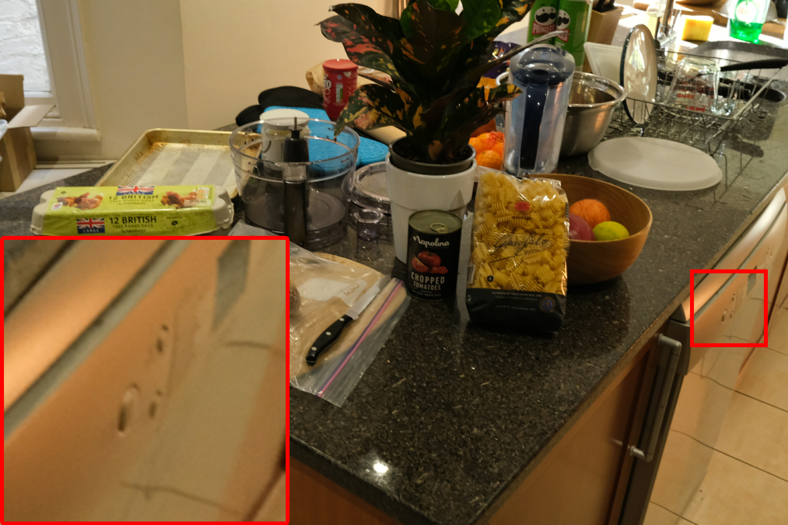
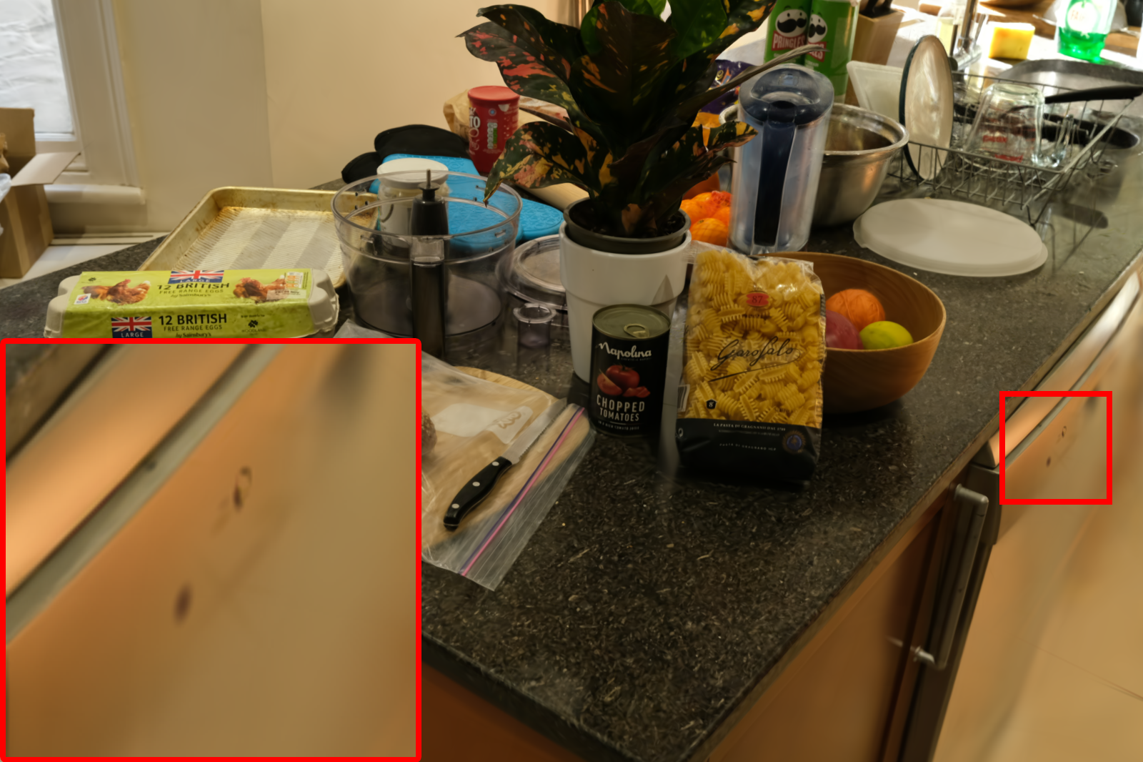
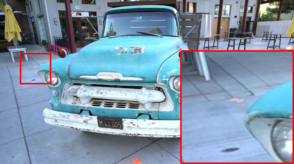
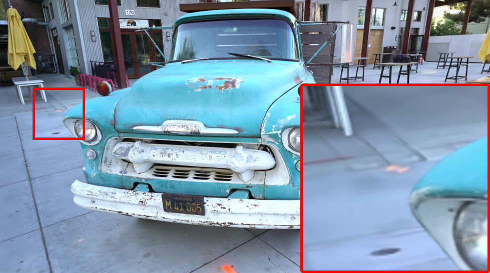
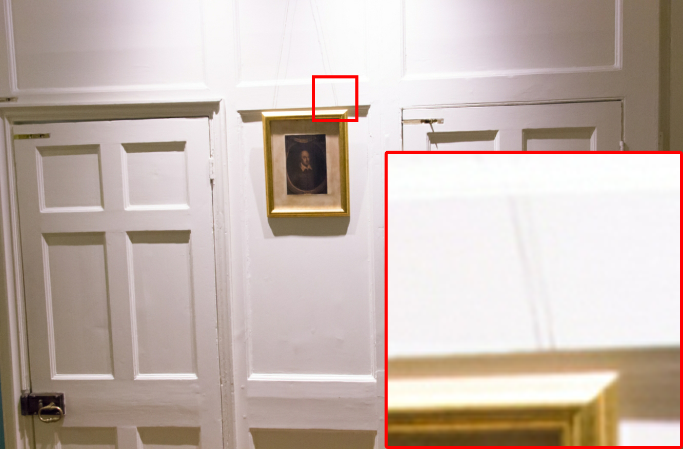
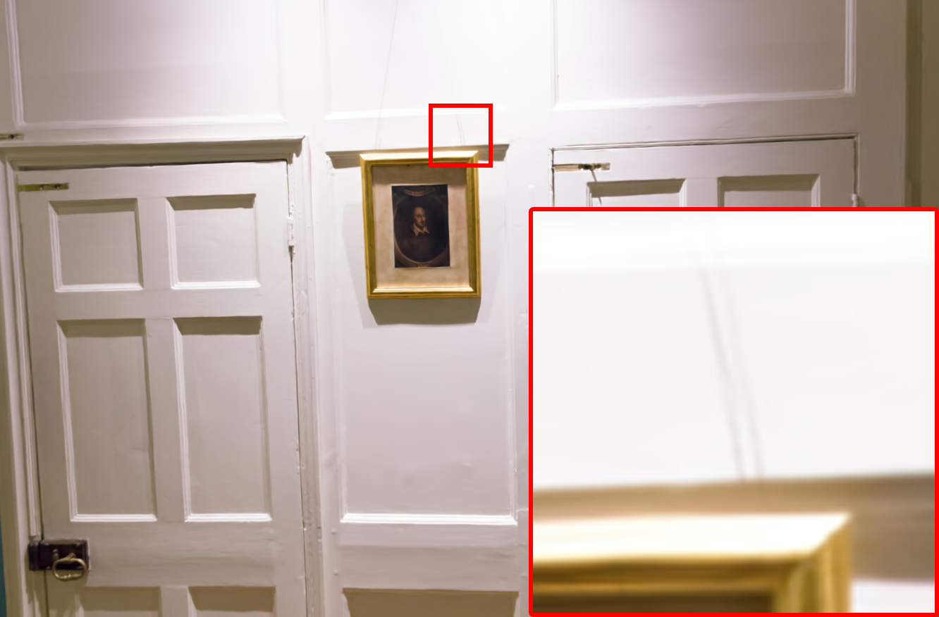
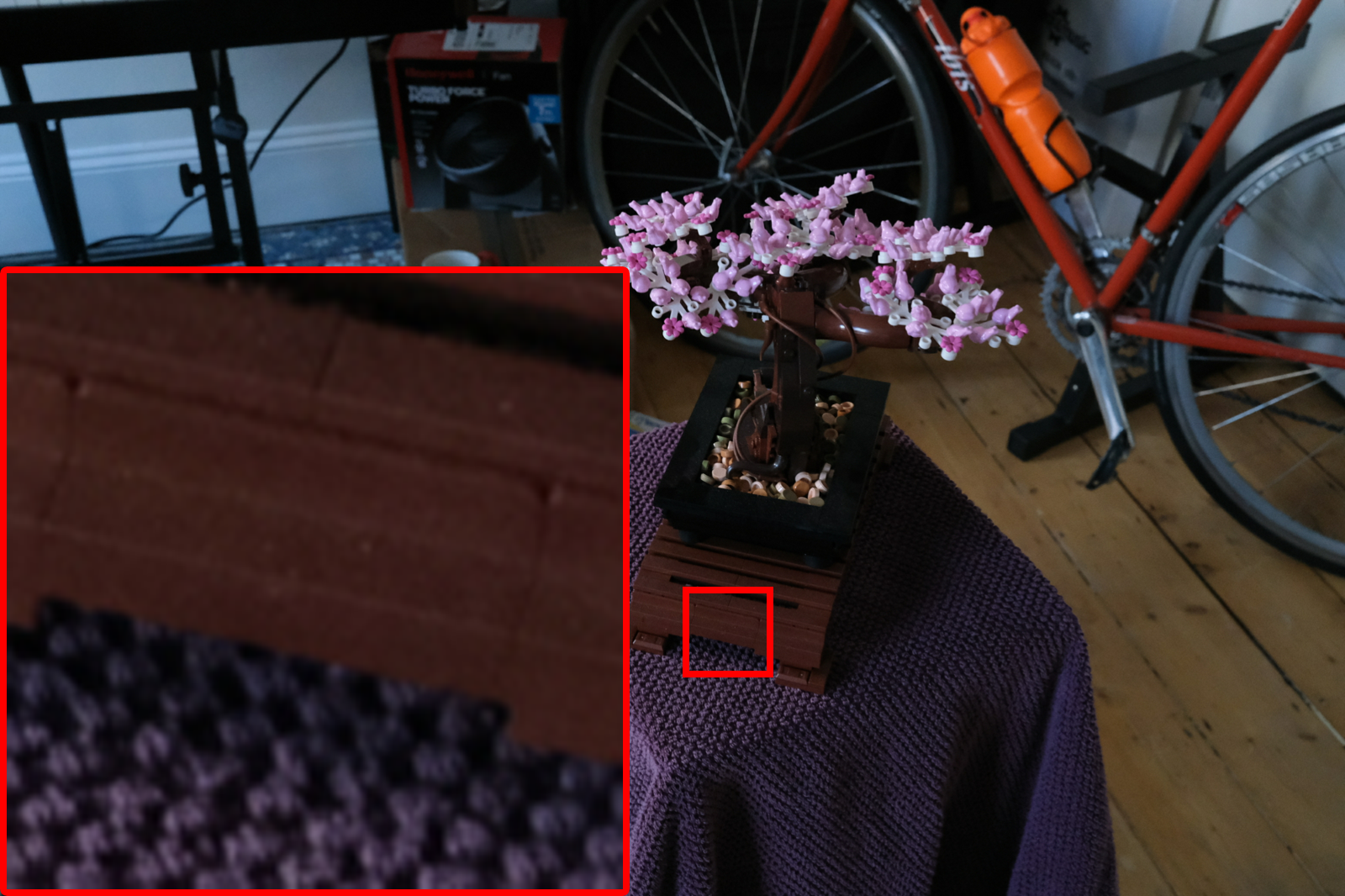
Figure 6: Qualitative Visualization Across 3DGS and raised cosine splatting. Displayed are side-by-side comparisons across the Counter, Truck, DrJohnson, Bonsai scenes (top to bottom) repsectively from Mip-NeRF 360, Tanks&Temples and Deep Blending datasets. In the Counter scene, raised cosines outperform Gaussians by better reconstructing the buttons, rendering them more prominently, whereas Gaussians struggle to achieve this even after full training. Similarly, in the Truck scene, raised cosines successfully reconstruct the orange mark on the floor, a detail that Gaussians fail to capture. In the Dr. Johnson scene, our method renders the string of the picture frame with greater clarity, closely resembling the ground truth imagery, while Gaussians fail to achieve the same level of detail. Lastly, in the Bonsai scene, the edges of the pot are more accurately represented by raised cosines as we can see its shadows, producing results that are closer to the ground truth image compared to those achieved with Gaussians. These examples highlight the advantages of raised cosine splatting in capturing finer details in 3D reconstruction compared to Gaussians.

9.2 Reduced Training Time

Figure 7: Comparison of Gaussian and $\cos\left(\frac{2\pi x^{2}}{36}\right)$ functions within the range $|x|\leq 3$ (same variance for both).

According to Fig.  7, which shows the half-cosine square with $\beta=2$ and $\xi=36$, along with the Gaussian 1D plot, we can observe that for a single primitive with the same variance, the cosine function can provide higher opacity values. Instead of requiring multiple splats to composite to determine the final pixel color, the cosine function can achieve the same accumulated value required with fewer primitives. Although the cosine function’s computation is more time-intensive compared to the Gaussian calculations, the overall training time is reduced due to the lower number of primitives required.

This is further illustrated in Figures 8 and 9, which provide a detailed analysis of the training loss and speed curves across various dataset scenes. Overall, despite having similar training loss curves with 3DGS, half-cosine splatting demonstrates superior performance compared to Gaussians.

9.3 Reduced Memory Usage

As previously mentioned, half cosine squared splatting specifically requires fewer primitives compared to Gaussians. This results in lower memory usage, as they provide higher opacity values across most of the regions they cover. In contrast, Gaussians require more primitives to achieve a similar accumulated opacity coverage. By using fewer half cosine squared primitives, we can achieve the desired color representation in the image space more efficiently. Similarly, sinc splatting and inverse quadratic splatting also consume lesser memory compared to Gaussians. The results in Table  6 and Table  7 further showcase this.

10 Extended Results and Simulations

Extended results. As mentioned in our paper, we trained our models on a single NVIDIA GeForce RTX 4090 GPU and recorded the training time. Since the benchmark models from other papers [20, 15] were trained on different GPUs, we applied a scaling factor to ensure a fair comparison of training times with the original papers’ results. According to [24], the relative training throughput of the RTX 4090 GPU and other GPU models (specifically, the RTX 3090 and RTX A6000 GPUs) can be determined with respect to a 1xLambdaCloud V100 16GB GPU. By dividing the training time data by these values, we have presented our training time results in a fair and comparable manner in Table  3.

A detailed breakdown of our results across every scene in the Mip-NeRF 360 [2], Tanks&Temples [22], and Deep Blending [17] datasets, along with their average values per dataset, is provided in Table  6 and Table  7. These results pertain to the selected DARB-Splatting algorithms, namely raised cosine splatting (3DRCS), half-cosine squared splatting (3DHCS), sinc splatting (3DSS), and inverse quadratic splatting (3DIQS). Key evaluation metrics, including PSNR, SSIM, LPIPS, memory usage, and training time for both 7k and 30k iterations, are analyzed in detail. These are presented alongside the results from implementing the updated codebase of 3DGS on our single NVIDIA GeForce RTX 4090 GPU to ensure a fair comparison. Our pipeline is anchored on this updated codebase, which produces improved results compared to those reported in the original 3DGS paper [20]. As shown in the tables, each DARB-Splatting algorithm demonstrates unique advantages in different utilities.

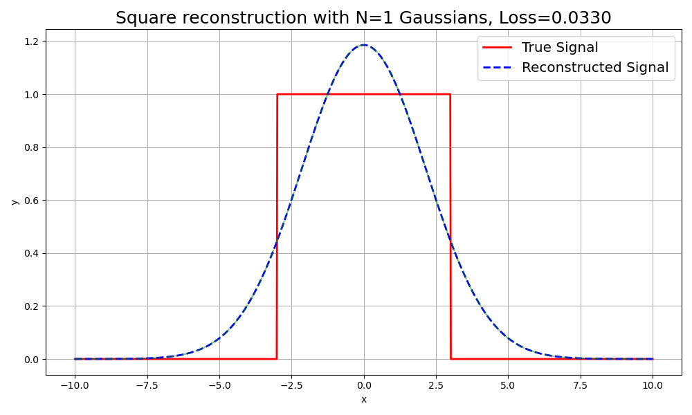
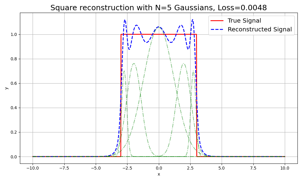
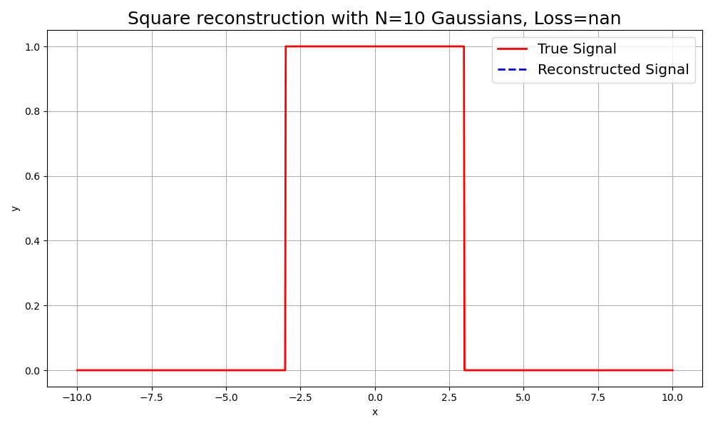
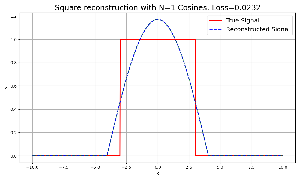
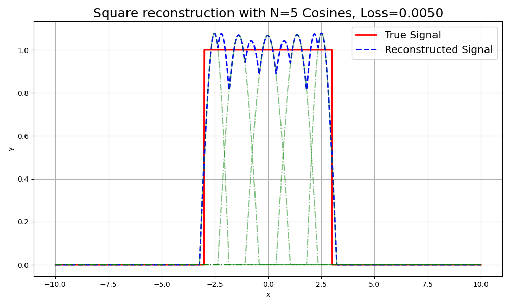
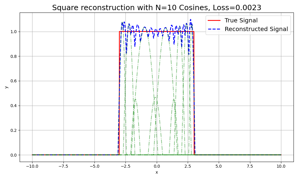
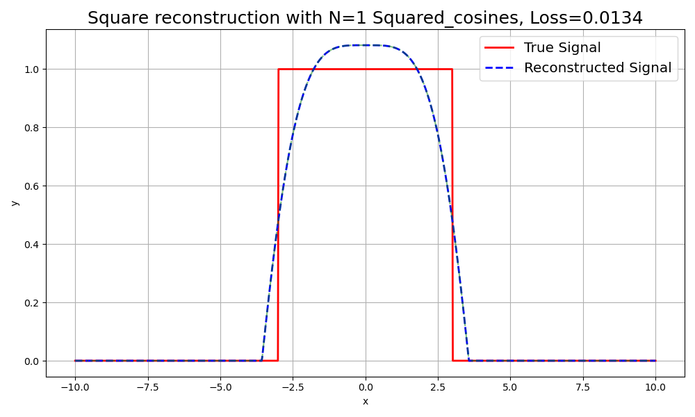
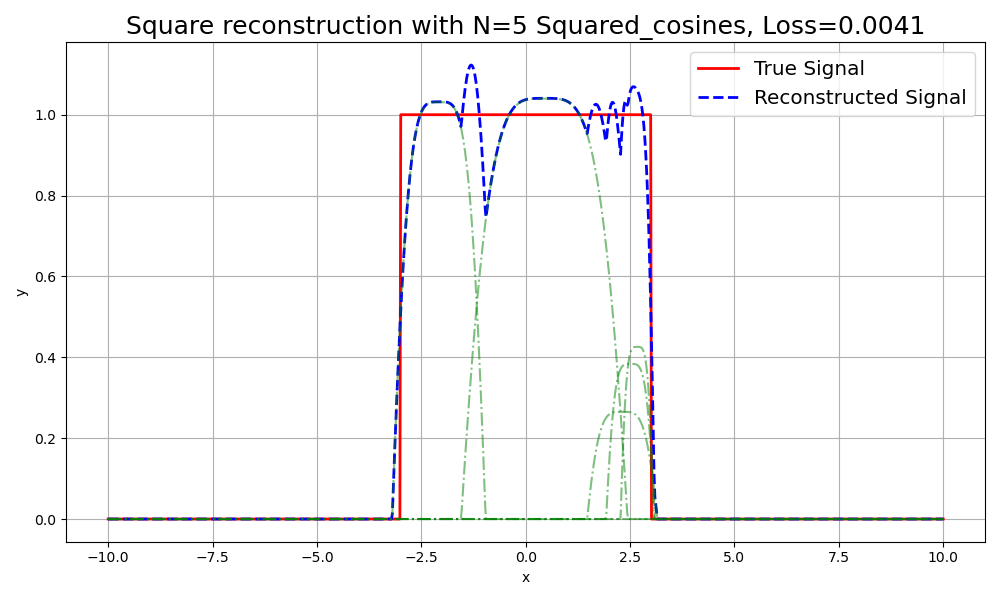
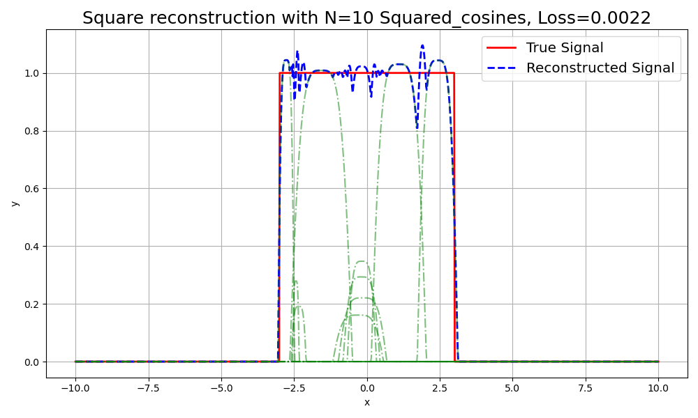
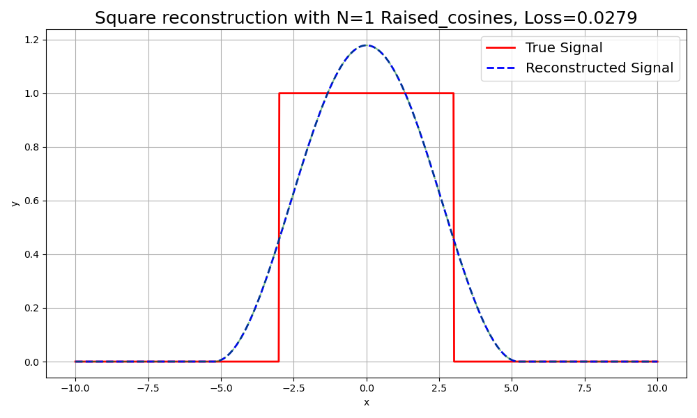
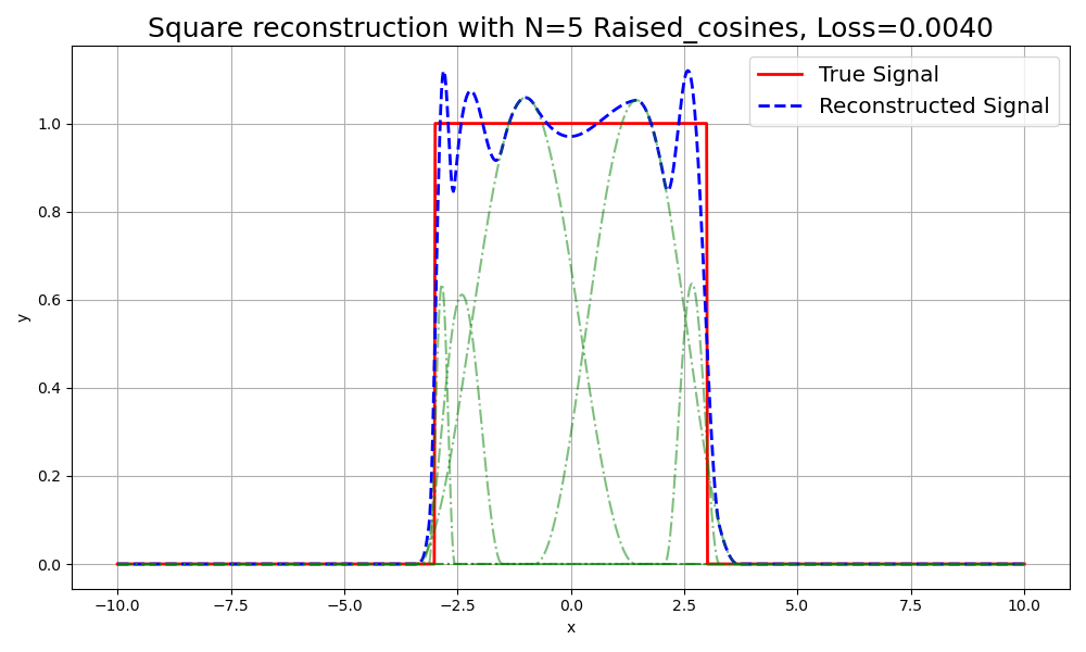
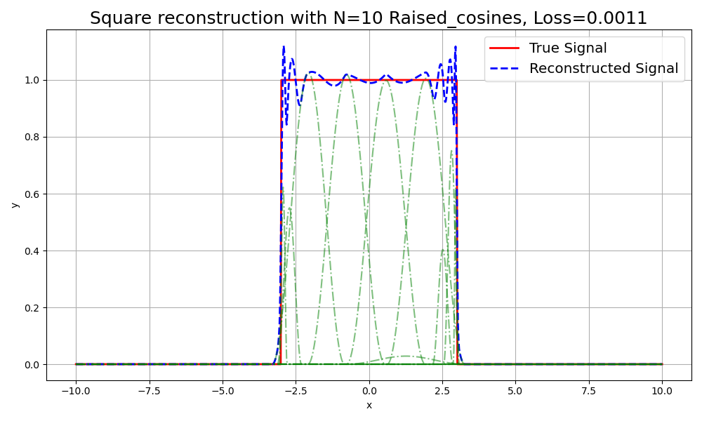
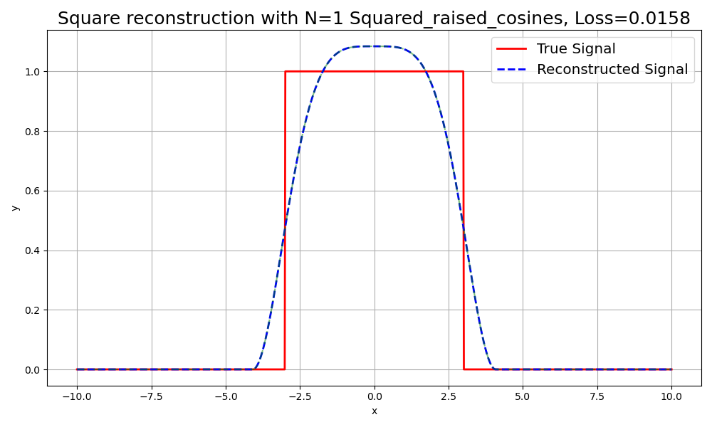
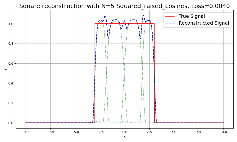
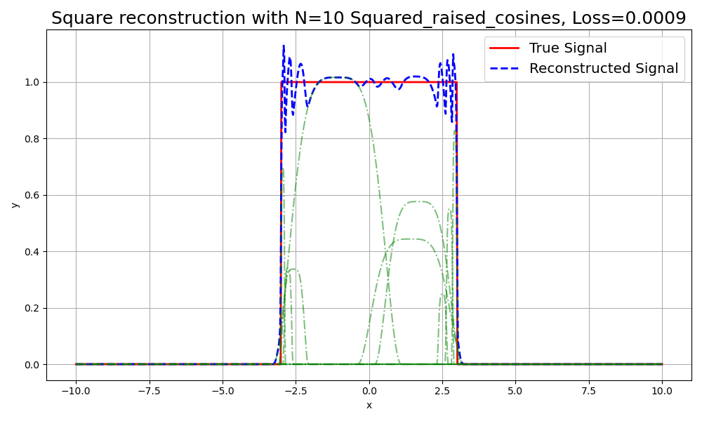
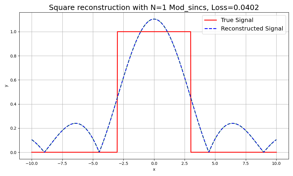
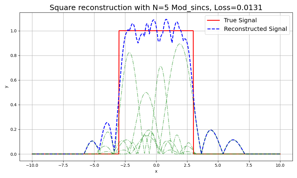
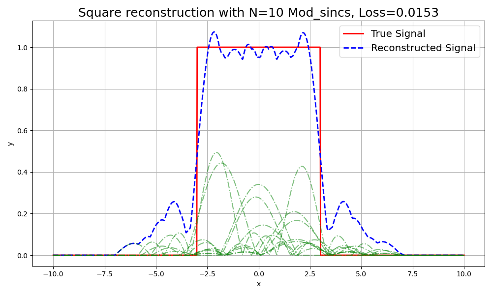
Figure 10: Visualization of 1D simulations for different splatting methods with varying primitives (N=1, N=5, N=10) for a square pulse. Each row corresponds to a specific splatting method: Gaussian, Cosine, Squared Cosine, Raised Cosine, Squared Raised Cosine, and Modulated Sinc. The columns represent the number of primitives used.

1D Simulations. In Figures  10,  11,  12,  13,  14,  15,  16, we show an extended version of the initial 1D simulation described in Sec. 3.2 in our paper. Here, we conduct experiments with various reconstruction kernels in 1D as a toy experiment to understand their signal reconstruction properties. These kernels include Gaussians, cosines, squared cosines, raised cosines, squared raised cosines, and modulus sincs. The reconstruction process is optimized using backpropagation, with different means and variances applied to each kernel. This approach is used to reconstruct various complex signal types, including a square pulse, a triangular pulse, a Gaussian pulse, a half-sinusoid single pulse, a sharp exponential pulse, a parabolic pulse, and a trapezoidal pulse.

We are grateful to the authors of GES [15] for open-sourcing their 1D simulation codes, which we have improved upon for this purpose. Expanding beyond GES, here, we also demonstrate the reconstruction of non-symmetric 1D signals to better represent real-world 3D reconstructions and further explore the capabilities of various DARBFs. As shown in the simulations, Gaussians are not the only effective interpolators; other DARBFs can provide improved 1D signal reconstructions in specific cases.

Train Loss

Train Speed

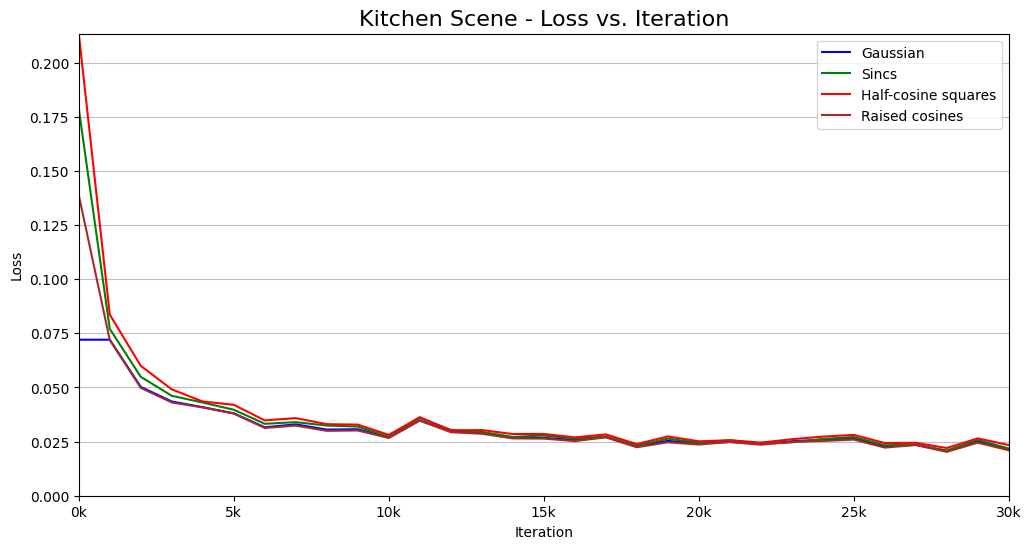
Kitchen

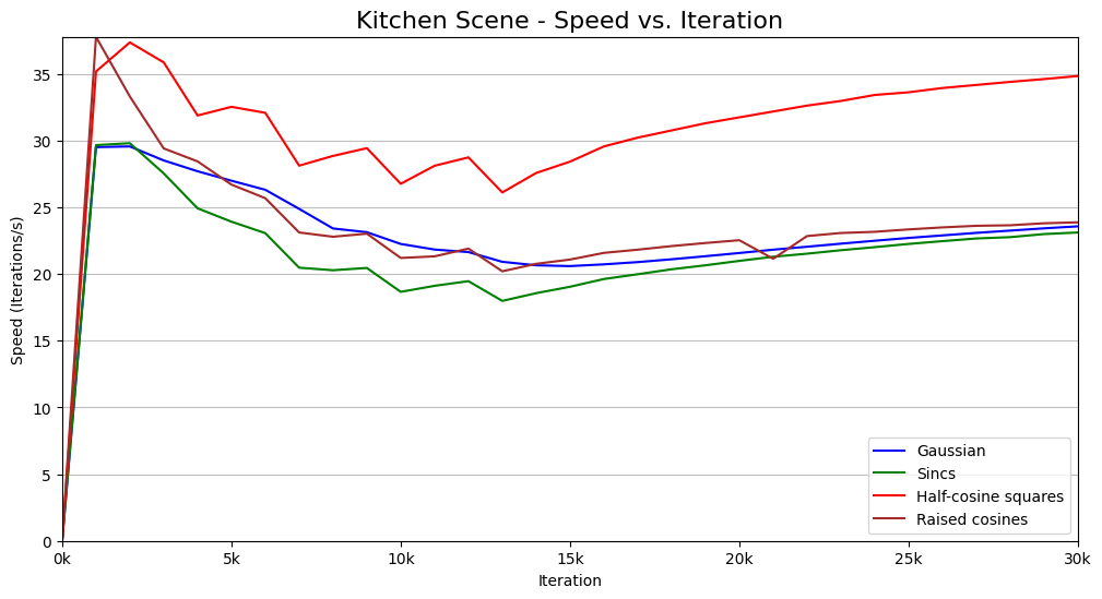
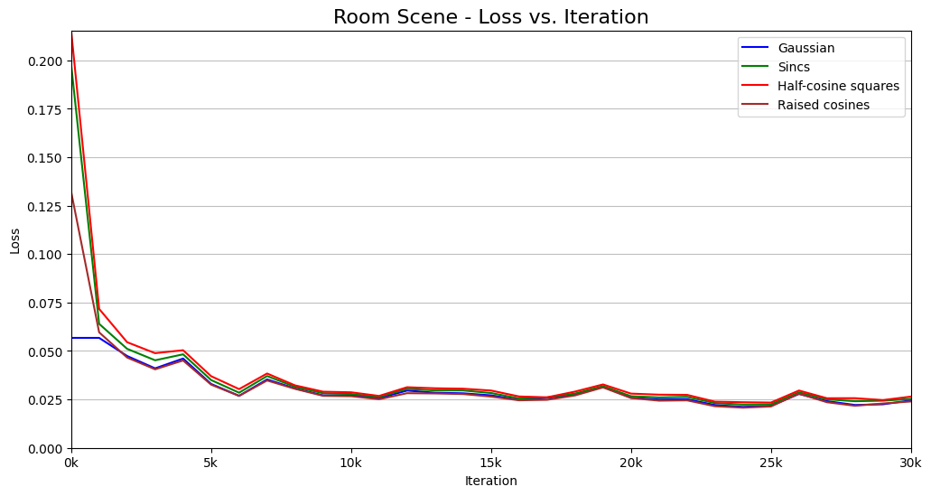
Room

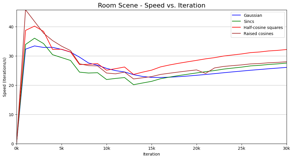
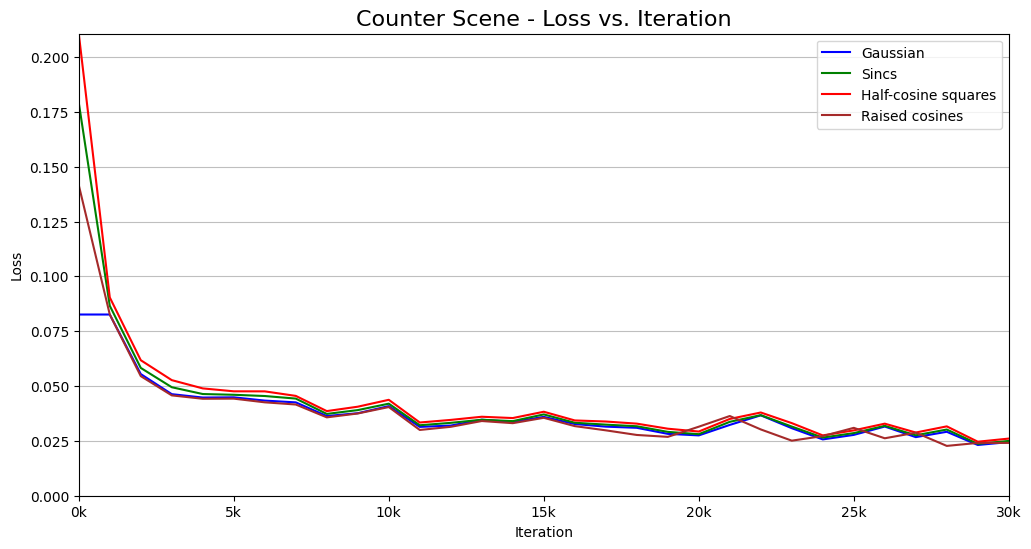
Counter

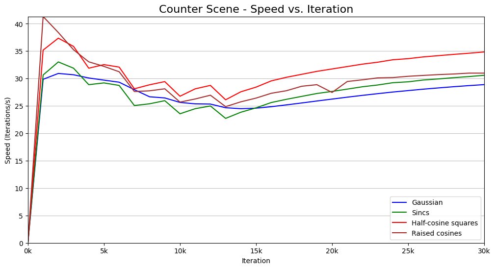
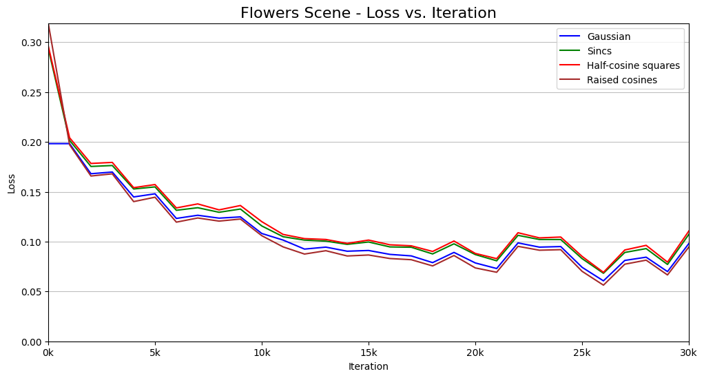
Flowers

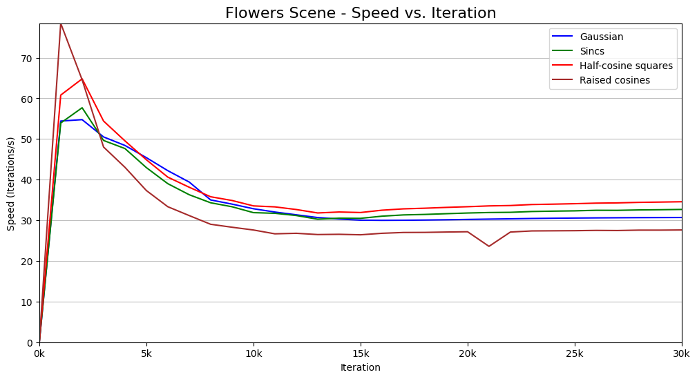
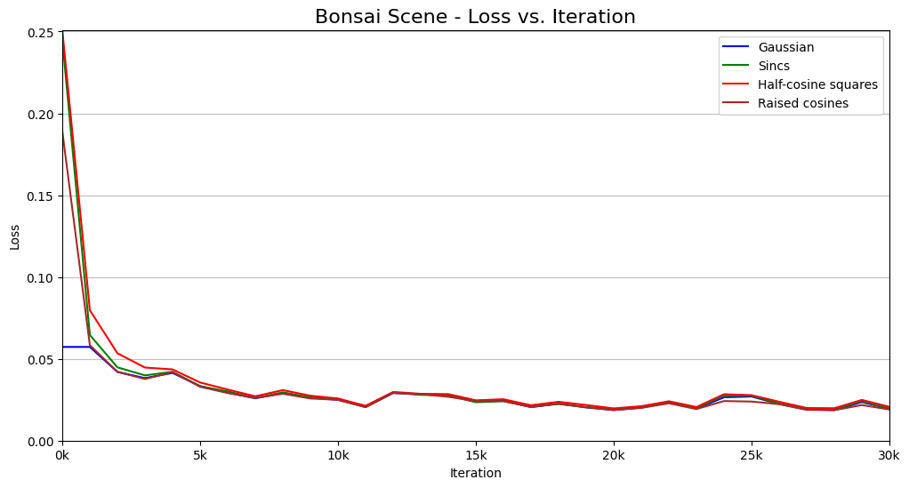
Bonsai

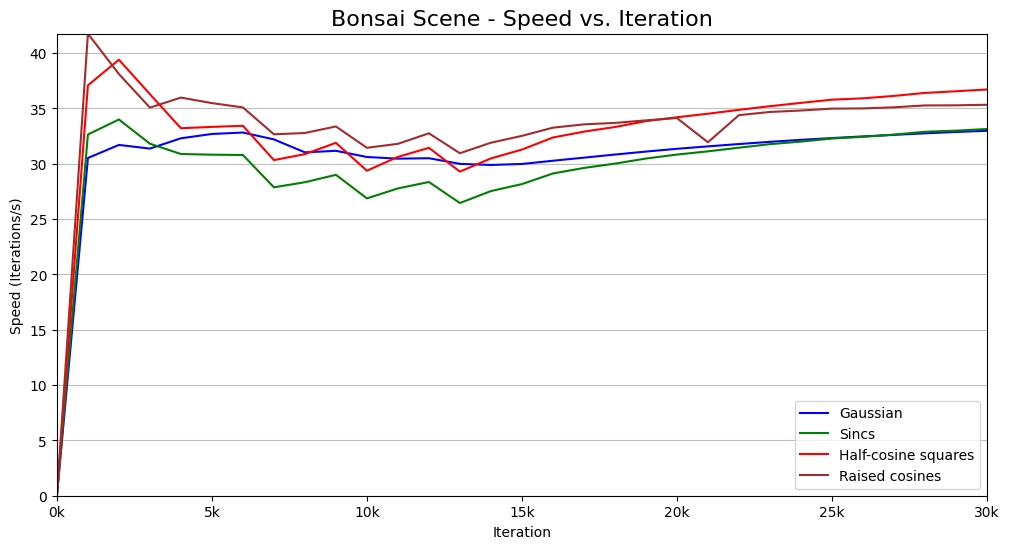
Figure 8: Training loss and speed curves across different scenes reveal significant performance differences. Specifically, the superior convergence speed of half-cosine squared splatting stands out compared to other selected DARBFs, particularly the Gaussian function. Although all the selected functions exhibit similar loss curves, notable variations are observed in their respective training speed curves across various scenes. These differences can be attributed to the inherent characteristics of each scene, which influence the training dynamics of the functions.

Train Loss

Train Speed

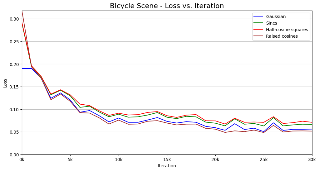
Bicycle

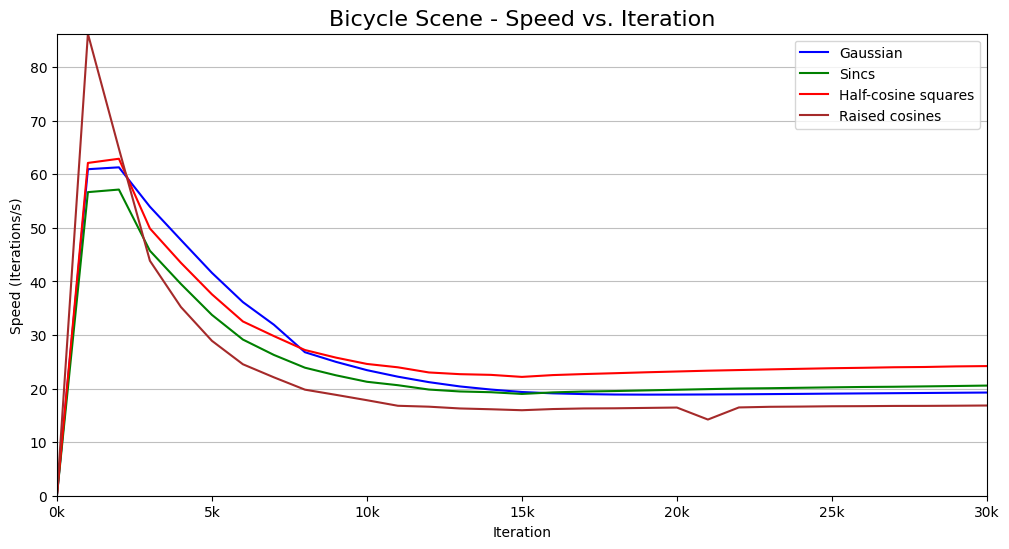
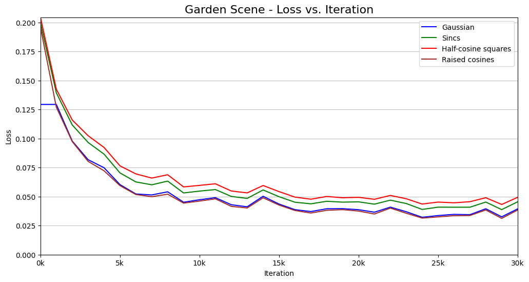
Garden

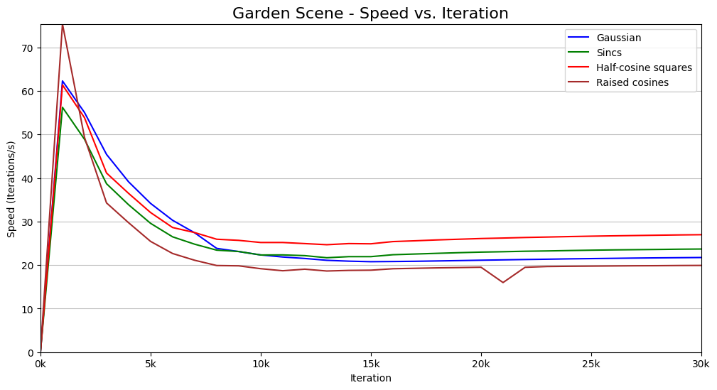
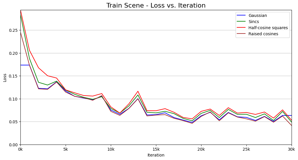
Train

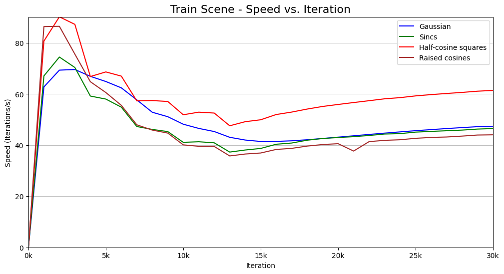
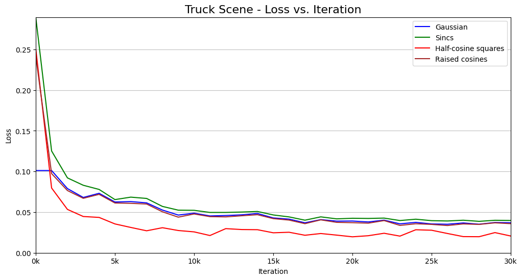
Truck

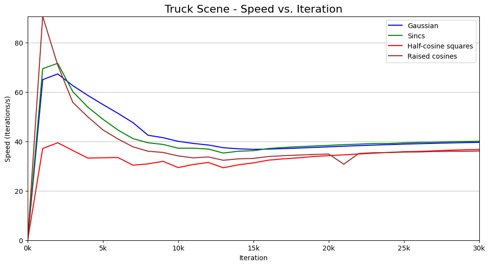
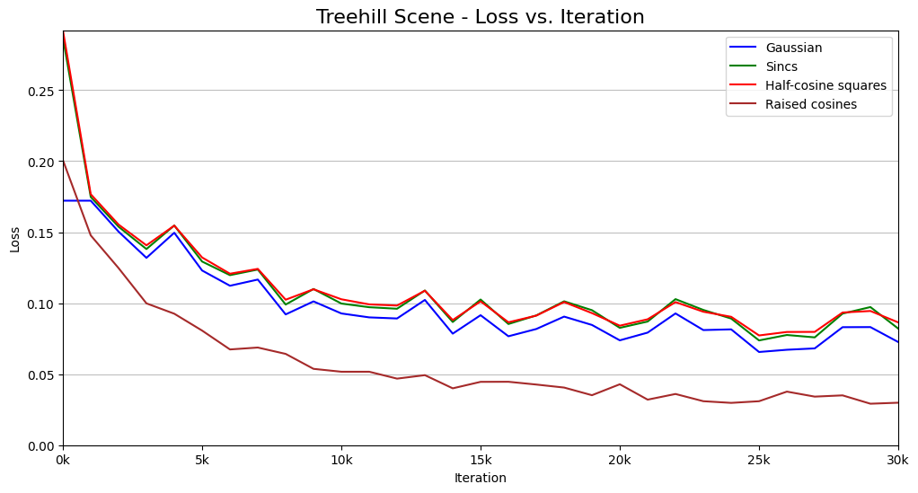
Treehill

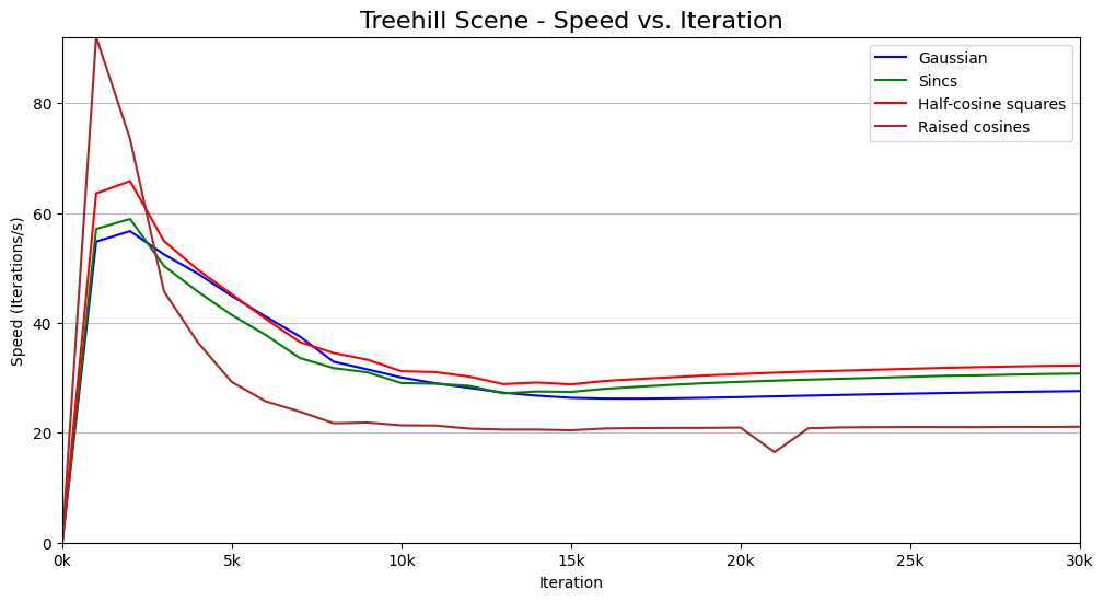
Figure 9: Training loss and speed curves across different scenes reveal significant performance differences. As an exception, in the Truck scene, we observe that the speed curves of Gaussians and raised cosines overlap and outperform half-cosine squares. However, when considering the overall performance across all scenes, half-cosine squares demonstrates superior efficiency in training time.

Table 6: Performance metrics across various scenes. Red color denotes best performance, while yellow denotes third-best. Higher values are better for PSNR, SSIM, and lower values are better for LPIPS, Memory, and Training Time. Here we present a detailed breakdown of results for all scenes from Mip-NeRF360 [2] dataset for 7k and 30k iterations. The performance of each model is heavily affected by the nature of the scene. Some values may differ from the main table due to stochastic processes, as these results are from a single instance of a full evaluation experiment series. In contrast, Table 3 presents the mean results averaged across multiple experiments.

Metric	Model	Step	Bicycle	Flowers	Garden	Stump	Treehill	Room	Counter	Kitchen	Bonsai	Mean
PSNR (dB)	3DGS	7k	23.759	20.4657	26.21	25.712	22.09	29.439	27.179	29.213	29.863	25.9525
		30k	25.248	21.519	27.352	26.562	22.554	31.597	29.055	31.378	32.316	27.4509
	3DRCS	7k	23.81	20.52	26.274	25.825	22.09	29.3625	27.261	29.312	29.635	26.0058
		30k	25.222	21.492	27.374	26.542	22.456	31.342	29.032	31.431	31.842	27.4547
	3DHCS	7k	23.037	19.929	25.351	24.821	22.078	29.127	26.837	28.756	29.481	25.4607
		30k	24.369	21.046	26.585	25.937	22.564	31.003	28.782	31.95	31.89	27.0451
	3DSS	7k	23.371	20.177	25.685	25.2	22.134	29.373	27.078	28.88	29.805	25.7447
		30k	24.813	21.2706	26.985	26.262	22.619	31.467	28.982	31.094	32.213	27.3006
	3DIQS	7k	23.309	19.782	25.669	24.893	21.591	28.986	26.71	28.211	28.132	25.2536
		30k	24.885	20.838	26.838	26.169	22.389	31.185	28.547	30.34	30.173	26.8182
LPIPS	3DGS	7k	0.328	0.422	0.16	0.294	0.418	0.26	0.2455	0.157	0.236	0.2801
		30k	0.211	0.342	0.108	0.217	0.33	0.22	0.202	0.126	0.205	0.2178
	3DRCS	7k	0.3197	0.41	0.156	0.283	0.406	0.257	0.241	0.155	0.231	0.2732
		30k	0.2079	0.334	0.108	0.212	0.324	0.219	0.2	0.126	0.203	0.2148
	3DHCS	7k	0.403	0.458	0.233	0.35	0.46	0.2787	0.256	0.168	0.238	0.3161
		30k	0.281	0.368	0.156	0.26	0.375	0.234	0.208	0.132	0.206	0.2466
	3DSS	7k	0.374	0.444	0.206	0.328	0.444	0.271	0.25	0.164	0.237	0.302
		30k	0.249	0.359	0.135	0.241	0.356	0.229	0.205	0.129	0.206	0.2343
	3DIQS	7k	0.355	0.462	0.18	0.335	0.443	0.268	0.253	0.17	0.242	0.3008
		30k	0.238	0.281	0.126	0.248	0.358	0.228	0.21	0.134	0.21	0.2258
SSIM	3DGS	7k	0.669	0.523	0.826	0.722	0.586	0.894	0.875	0.903	0.92	0.7686
		30k	0.763	0.6	0.863	0.769	0.633	0.917	.903	0.9256	0.939	0.8125
	3DRCS	7k	0.6735	0.5302	0.8297	0.7283	0.5913	0.8953	0.8786	0.905	0.9214	0.7726
		30k	0.7641	0.6039	0.864	0.7703	0.6325	0.9176	0.906	0.9256	0.94	0.8137
	3DHCS	7k	0.602	0.478	0.771	0.668	0.557	0.883	0.866	0.894	0.915	0.7371
		30k	0.706	0.566	0.827	0.7337	0.61	0.91	0.898	0.92	0.9355	0.7895
	3DSS	7k	0.631	0.498	0.795	0.693	0.571	0.889	0.873	0.899	0.918	0.7508
		30k	0.736	0.583	0.845	0.752	0.623	0.914	0.903	0.923	0.938	0.8008
	3DIQS	7k	0.637	0.474	0.8	0.678	0.564	0.884	0.862	0.889	0.911	0.7443
		30k	0.739	0.555	0.843	0.742	0.615	0.909	0.894	0.914	0.928	0.7932
Memory (MB)	3DGS	7k	753	503	840	844	502	259	229	358	252	504
		30k	1135	658	950	1024	727	313	250	384	258	633
	3DRCS	7k	789	516	842	879	528	255	238	370	275	521
		30k	1120	668	953	1010	749	343	276	412	279	645
	3DHCS	7k	570	412	630	699	413	211	228	322	211	410
		30k	858	578	739	867	632	256	242	372	245	532
	3DSS	7k	592	424	672	706	396	240	223	364	266	431
		30k	948	586	800	901	602	281	250	393	272	559
	3DIQS	7k	394	263	484	478	245	153	140	223	149	281
		30k	608	373	518	611	375	182	151	238	153	356
Training time (s)	3DGS	7k	181	160	212	173	163	225	240	265	217	204
		30k	1378	920	1302	1149	1020	1178	1107	1313	949	1146
	3DRCS	7k	193	155	218	182	159	194	205	239	192	193
		30k	1581	995	1400	1292	1098	1087	1010	1247	876	1176
	3DHCS	7k	164	145	199	158	145	217	223	252	210	172
		30k	1103	806	1035	996	848	1002	934	1181	870	975
	3DSS	7k	182	153	202	169	157	233	243	281	185	201
		30k	1324	879	1215	1093	944	1200	1106	1413	1001	1130
	3DIQS	7k	161	146	186	152	155	238	263	269	223	199
		30k	1004	704	993	842	799	1105	1049	1261	880	960

Table 7: Performance metrics across various scenes. Red color denotes best performance, while yellow denotes third-best. Higher values are better for PSNR, SSIM, and lower values are better for LPIPS, Memory, and Training Time. Here we present a detailed breakdown of results for all scenes from Tanks&Temples [22] and Deep Blending [17] datasets for 7k and 30k iterations. The performance of each model is heavily affected by the nature of the scene. Some values may differ from the main table due to stochastic processes, as these results are from a single instance of a full evaluation experiment series. In contrast, Table 3 presents the mean results averaged across multiple experiments.

Metric	Model	Step	Tanks&Temples			Deep Blending
			Truck	Train	Mean	DrJohnson	Playroom	Mean
PSNR (dB)	3DGS	7k	23.933	19.795	21.784	27.609	29.354	28.4215
		30k	25.481	22.201	23.771	29.493	29.976	29.6645
	3DRCS	7k	24.026	19.758	21.882	27.437	29.417	28.477
		30k	25.314	22.077	23.6355	29.35	29.981	29.6355
	3DHCS	7k	22.851	19.391	21.071	26.844	28.965	27.9345
		30k	24.561	21.721	23.108	29.003	29.772	29.3875
	3DSS	7k	23.44	19.658	21.589	27.371	29.417	28.394
		30k	25.03	21.973	23.5065	29.414	29.955	29.6645
	3DIQS	7k	23.3	19.43	21.365	27.279	28.904	28.0915
		30k	24.83	21.856	23.343	29.239	29.769	29.504
LPIPS	3DGS	7k	0.197	0.318	0.2515	0.318	0.284	0.301
		30k	0.144	0.199	0.1725	0.237	0.243	0.24
	3DRCS	7k	0.19	0.312	0.251	0.3178	0.282	0.2999
		30k	0.1423	0.196	0.1661	0.238	0.2435	0.2407
	3DHCS	7k	0.235	0.354	0.2945	0.341	0.298	0.3195
		30k	0.169	0.231	0.2	0.25	0.256	0.253
	3DSS	7k	0.218	0.334	0.276	0.325	0.292	0.3085
		30k	0.159	0.218	0.1885	0.243	0.25	0.2465
	3DIQS	7k	0.213	0.34	0.2765	0.327	0.292	0.3095
		30k	0.154	0.221	0.1875	0.24	0.247	0.2435
SSIM	3DGS	7k	0.848	0.719	0.7815	0.87	0.894	0.882
		30k	0.88	0.818	0.851	0.903	0.903	0.903
	3DRCS	7k	0.8527	0.7242	0.7884	0.8696	0.8942	0.8819
		30k	0.8818	0.8197	0.8507	0.9015	0.9013	0.9014
	3DHCS	7k	0.813	0.684	0.7485	0.856	0.887	0.8715
		30k	0.858	0.791	0.8245	0.899	0.9	0.8995
	3DSS	7k	0.831	0.704	0.7675	0.866	0.891	0.8785
		30k	0.869	0.803	0.836	0.902	0.902	0.902
	3DIQS	7k	0.827	0.693	0.76	0.862	0.886	0.874
		30k	0.866	0.795	0.8305	0.902	0.899	0.9005
Memory (MB)	3DGS	7k	406	180	293	462	336	399
		30k	485	257	371	742	412	577
	3DRCS	7k	476	132	304	491	352	421.5
		30k	548	181	364.5	767	446	606.5
	3DHCS	7k	344	145	244.5	355	331	343
		30k	446	230	338	634	417	482.5
	3DSS	7k	355	156	255.5	399	316	357.5
		30k	434	232	333	682	400	541
	3DIQS	7k	236	114	175	299	197	248
		30k	291	156	223.5	489	239	364
Training time (s)	3DGS	7k	132	112	122	212	176	194
		30k	738	631	684.5	1385	1039	1212
	3DRCS	7k	134	105	119.5	193	162	177.5
		30k	793	660	726.5	1378	1023	1200.5
	3DHCS	7k	114	103	108.5	213	169	191
		30k	604	498	551	1163	947	1055
	3DSS	7k	131	118	124.5	219	176	197.5
		30k	745	659	702	1407	1087	1247
	3DIQS	7k	129	123	126	216	164	190
		30k	624	602	613	1262	918	1090

N=1

N=5

N=10

N=1

N=5

N=10

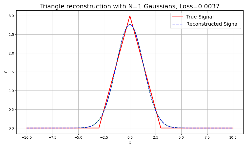
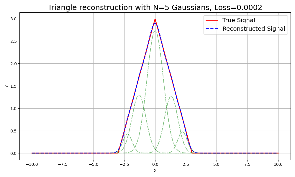
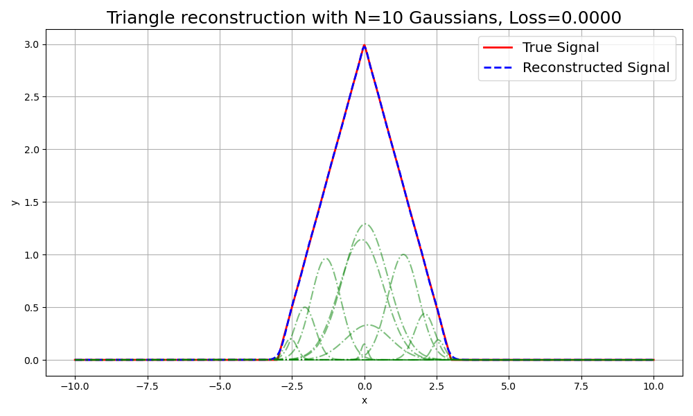
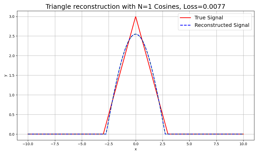
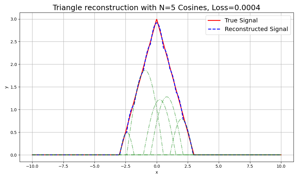
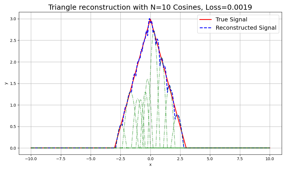
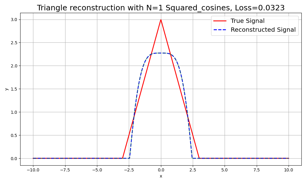
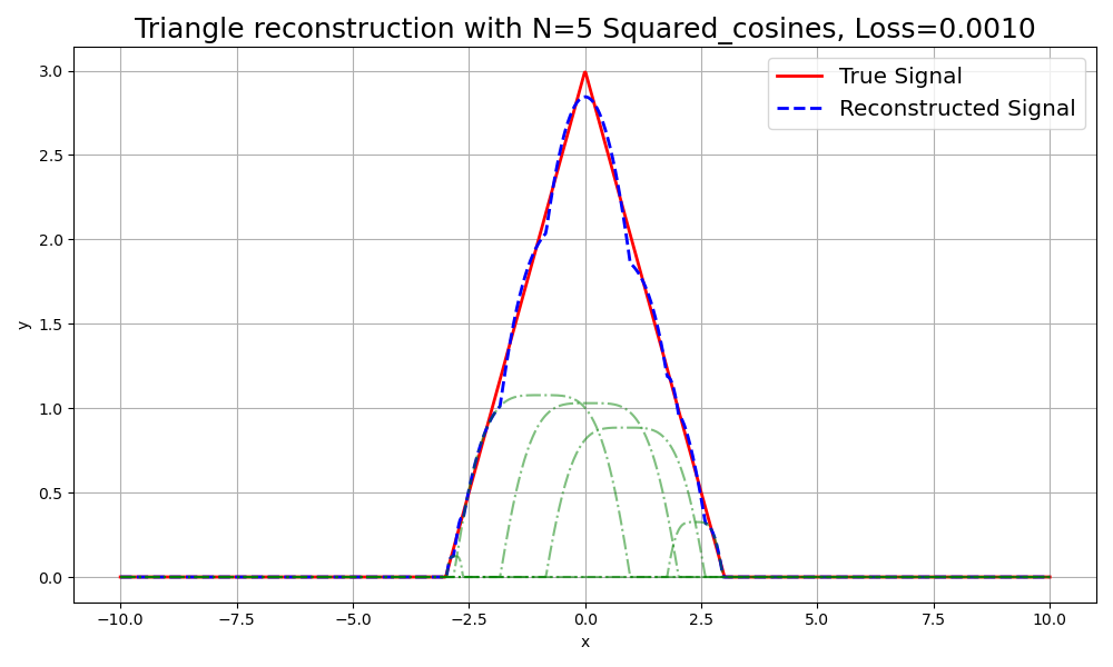
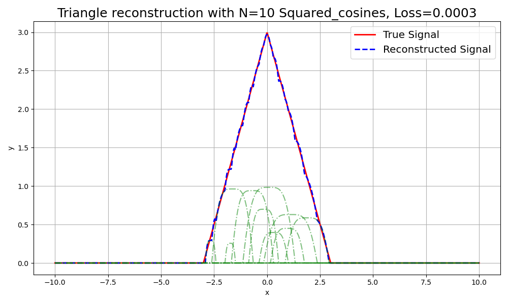
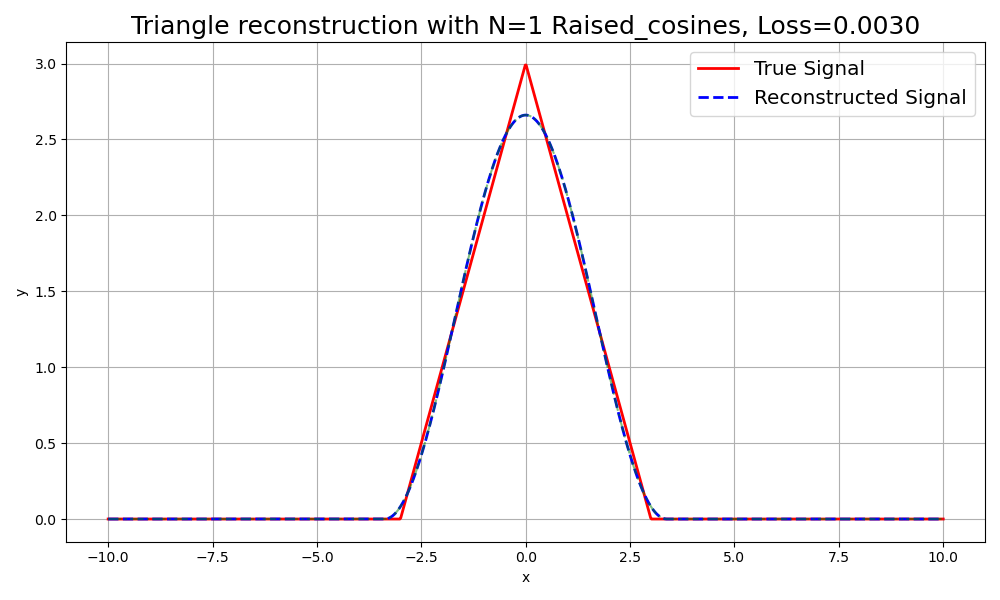
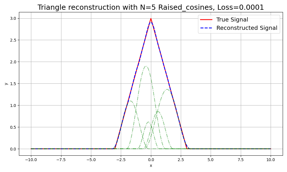
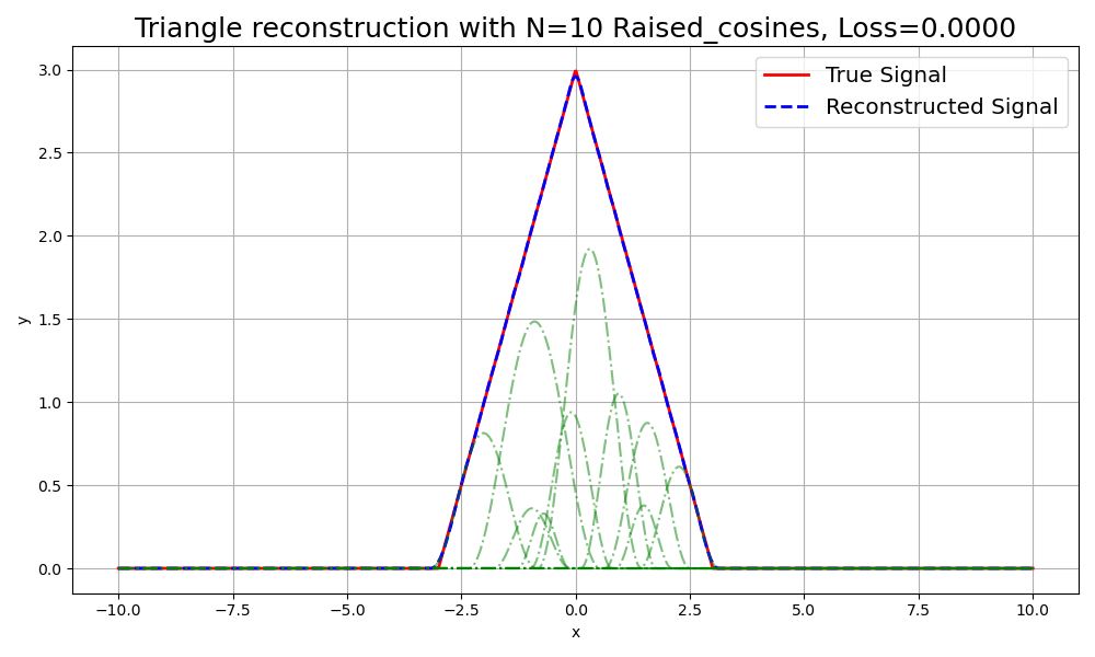
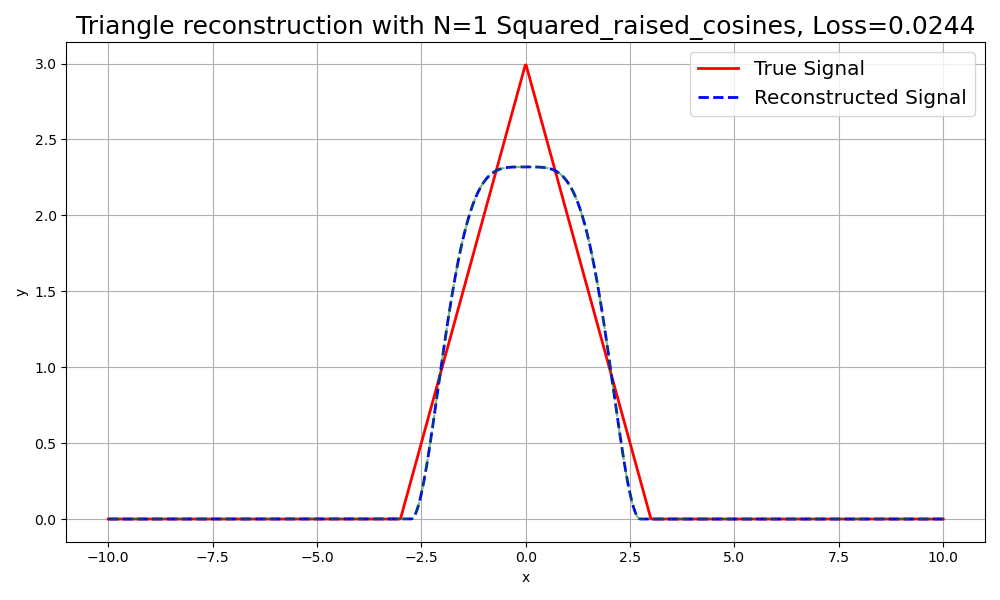
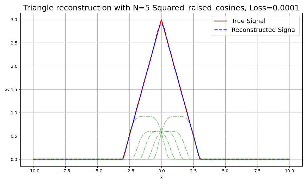
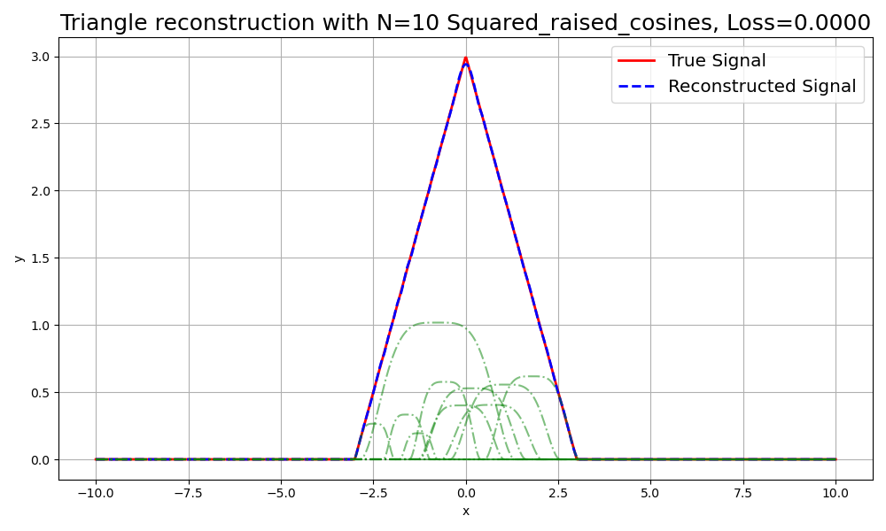
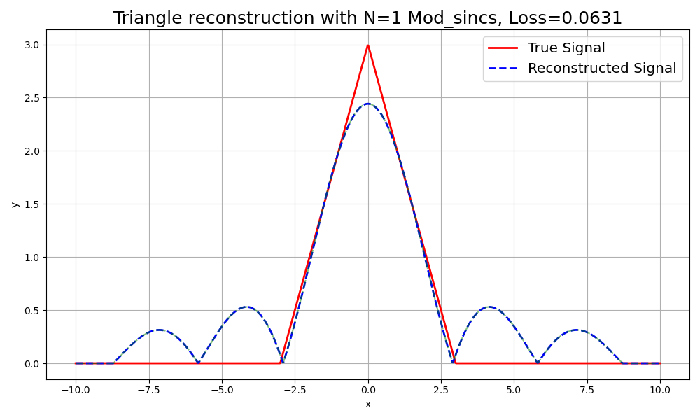
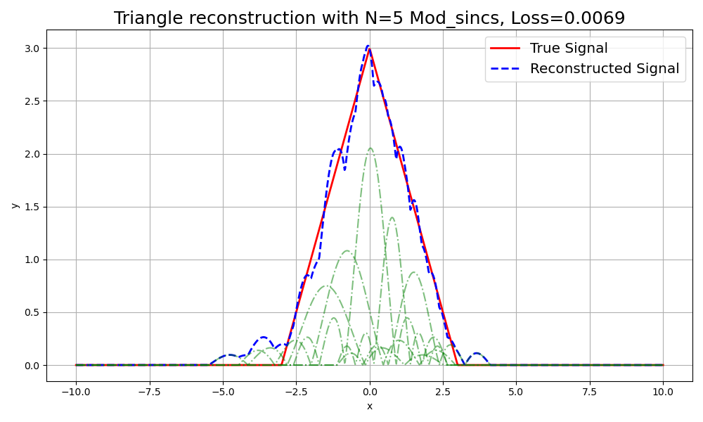
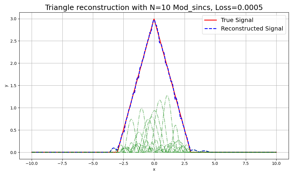
Figure 11: Visualization of 1D simulations for different splatting methods with varying primitives (N=1, N=5, N=10) for a triangle pulse. Each row corresponds to a specific splatting method: Gaussian, Cosine, Squared Cosine, Raised Cosine, Squared Raised Cosine, and Modulated Sinc. The columns represent the number of primitives used.

N=1

N=5

N=10

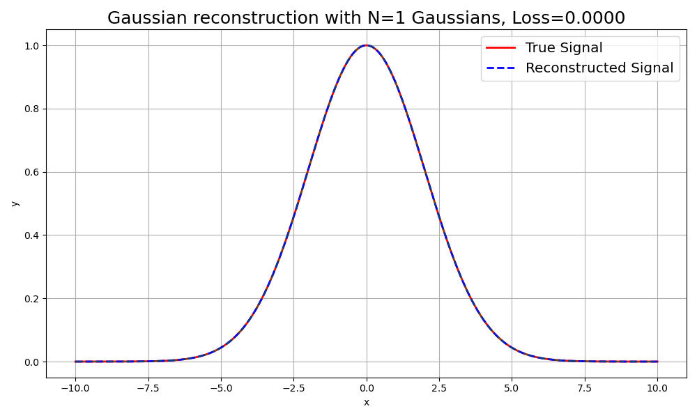
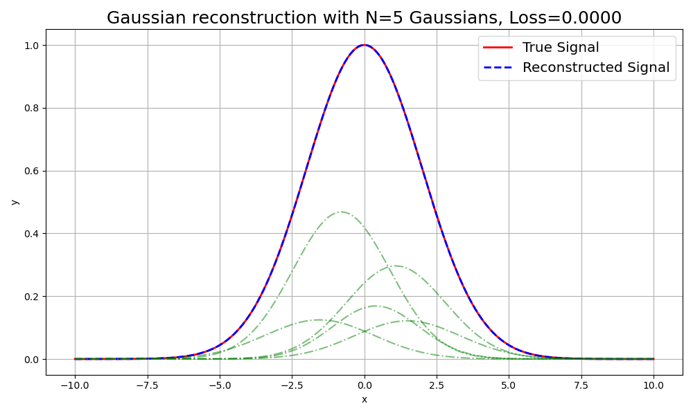
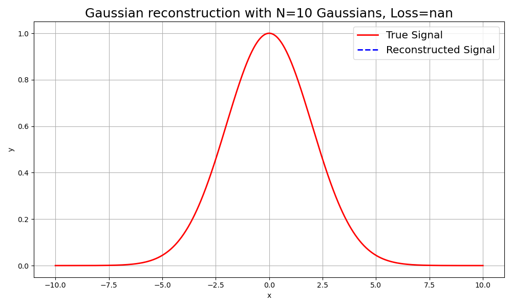
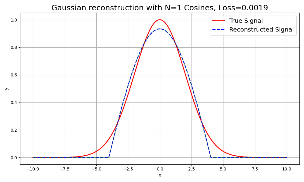
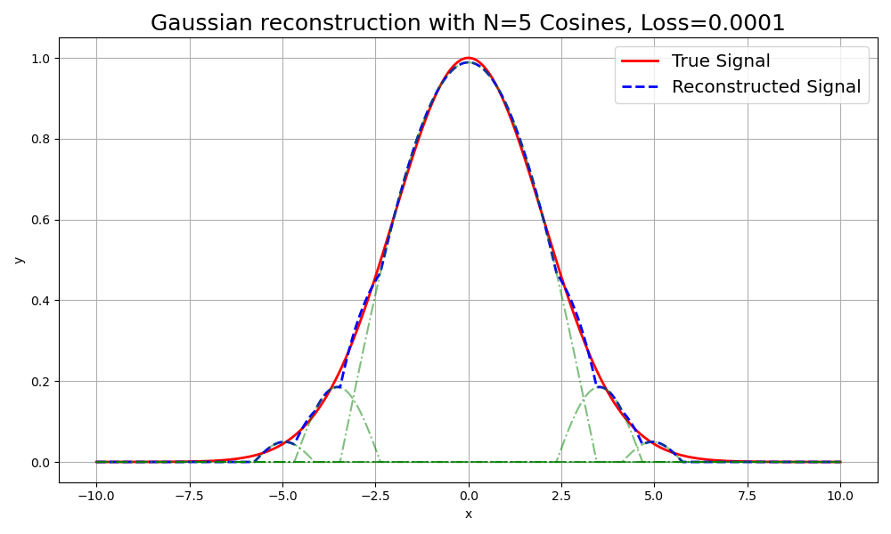
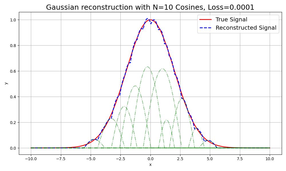
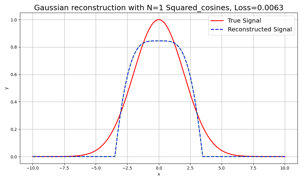
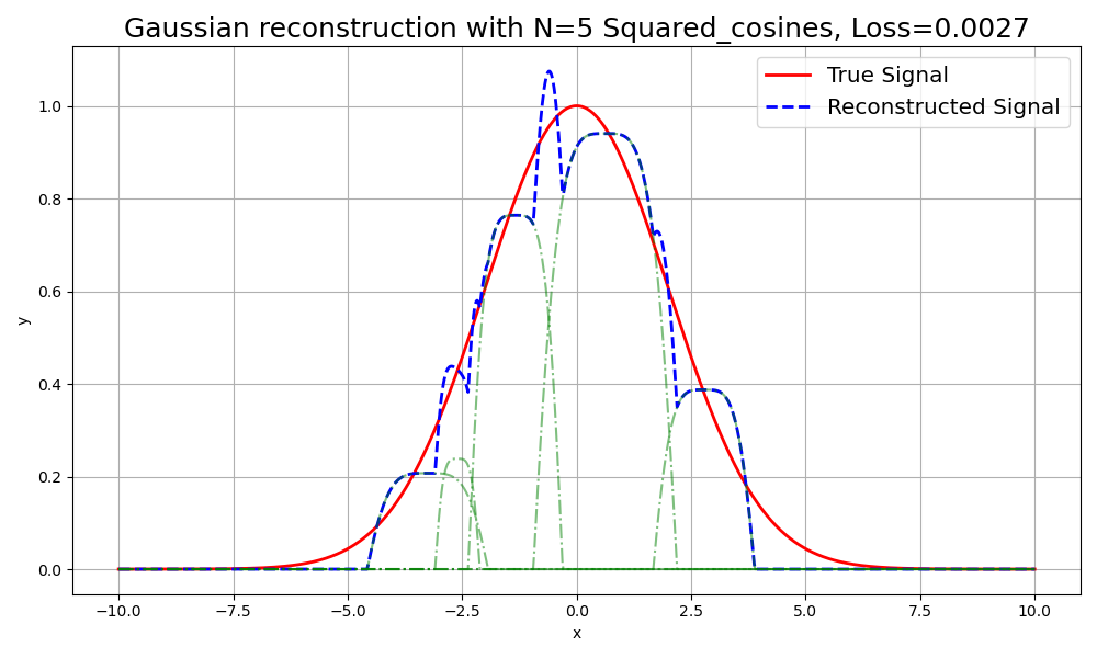
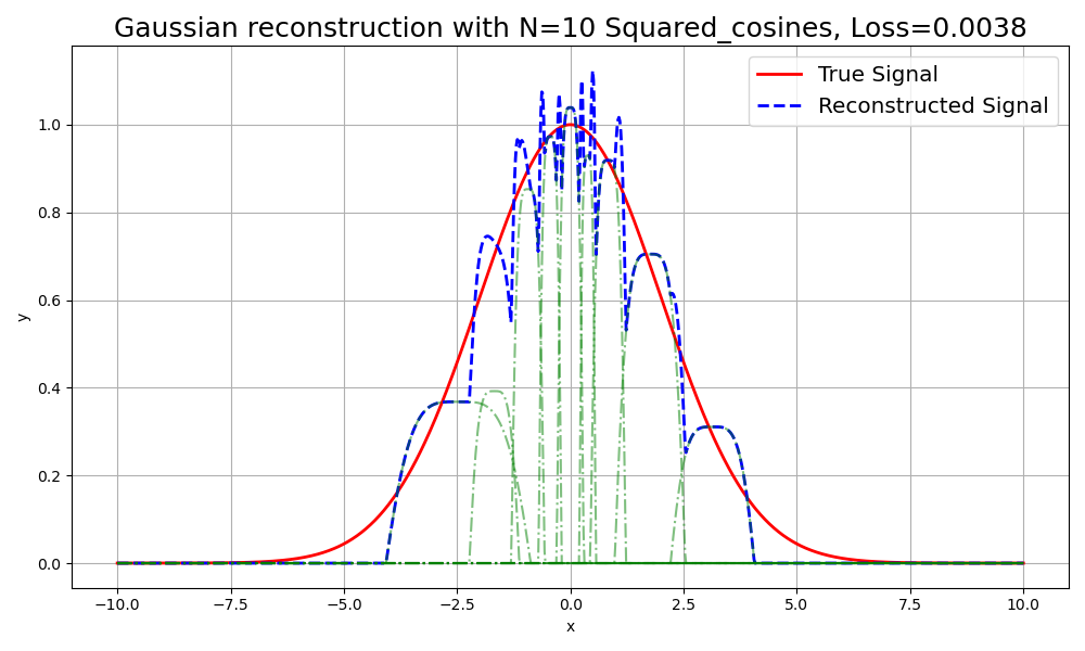
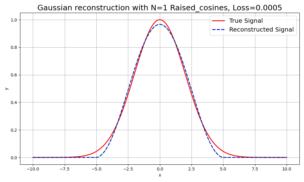
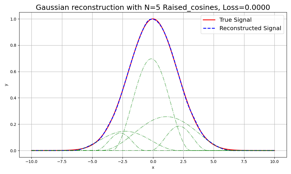
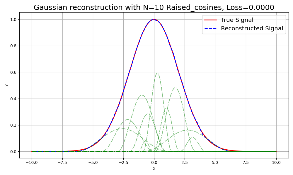
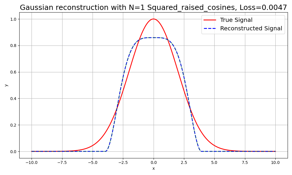
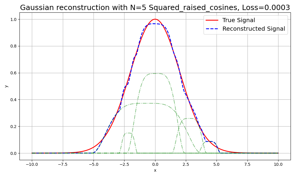
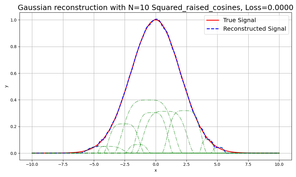
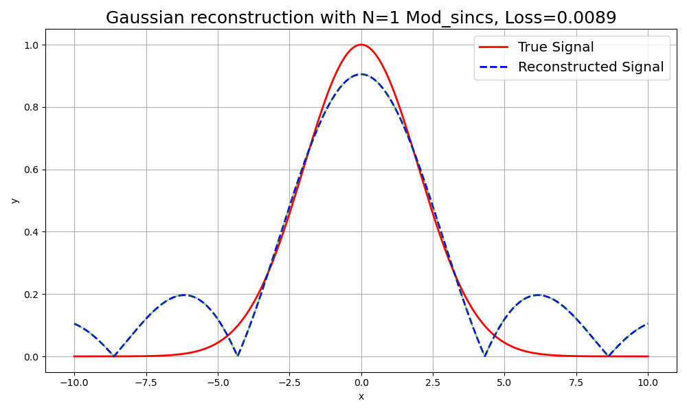
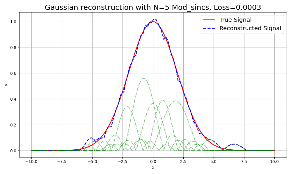
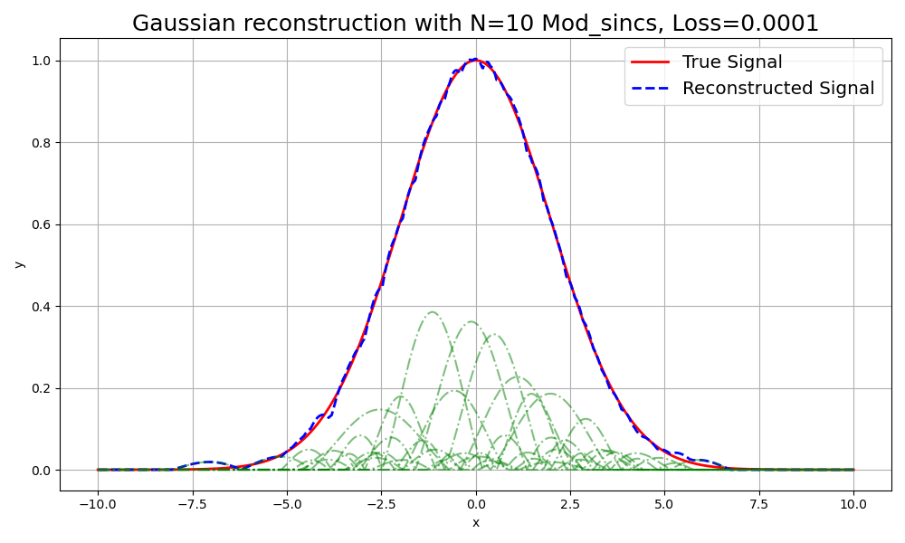
Figure 12: Visualization of 1D simulations for different splatting methods with varying primitives (N=1, N=5, N=10) for a Gaussian. Each row corresponds to a specific splatting method: Gaussian, Cosine, Squared Cosine, Raised Cosine, Squared Raised Cosine, and Modulated Sinc. The columns represent the number of primitives used.

N=1

N=5

N=10

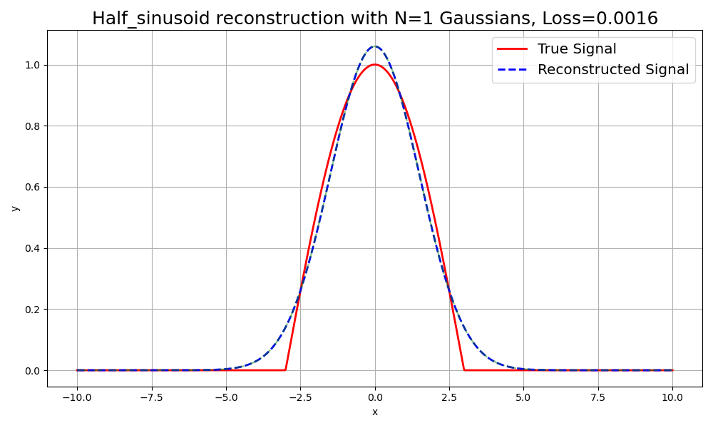
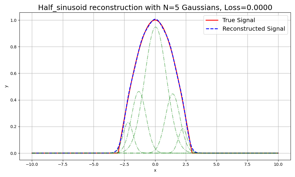
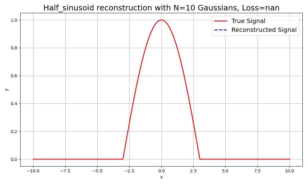
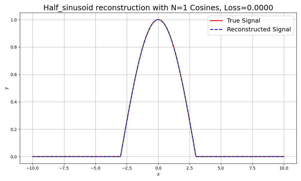
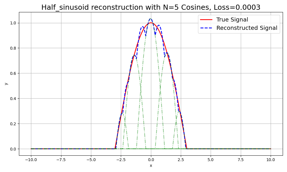
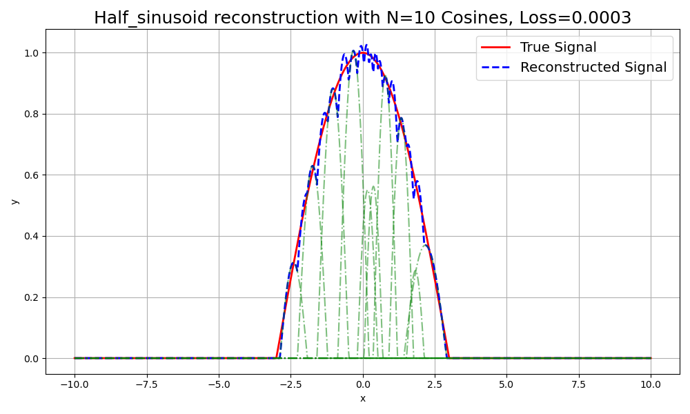
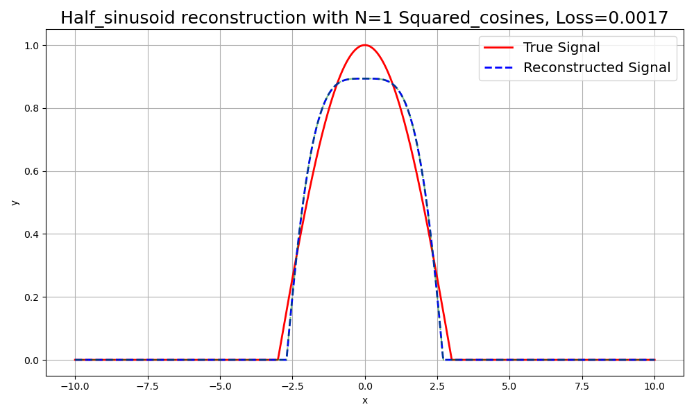
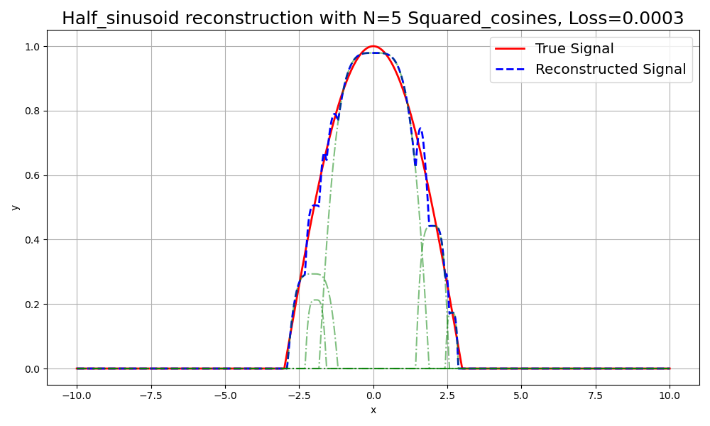
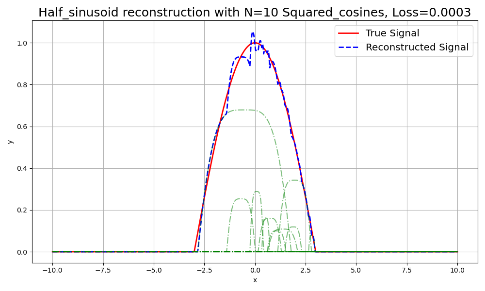
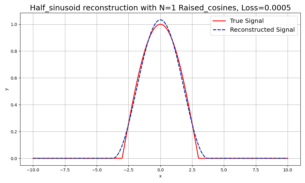
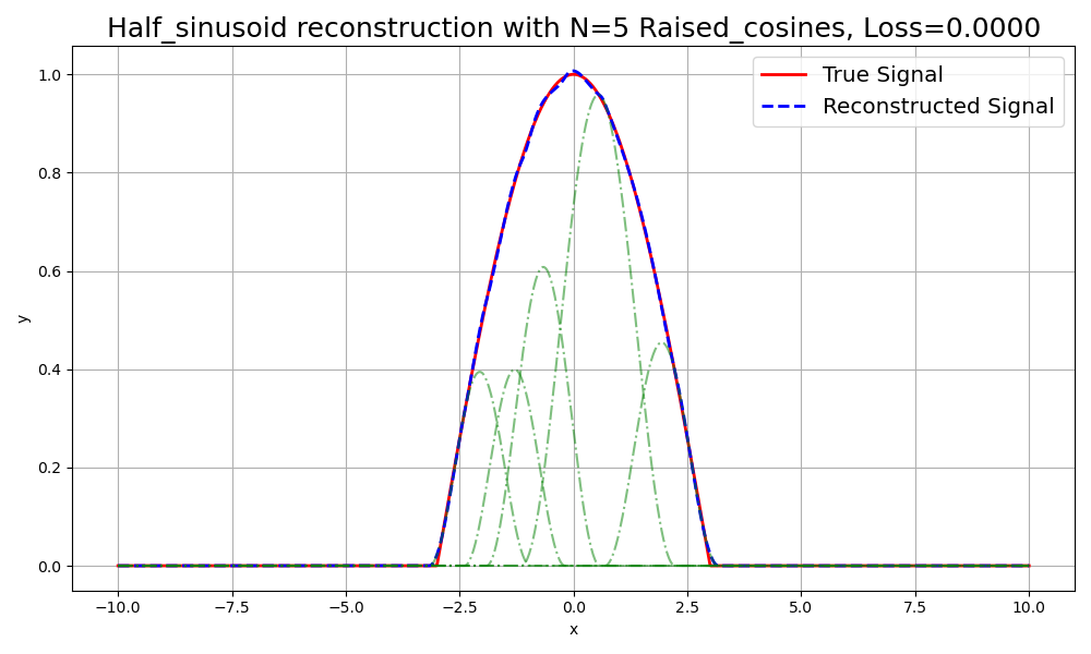
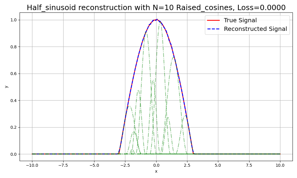
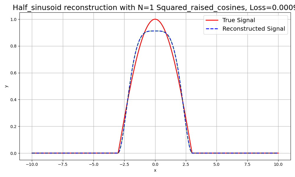
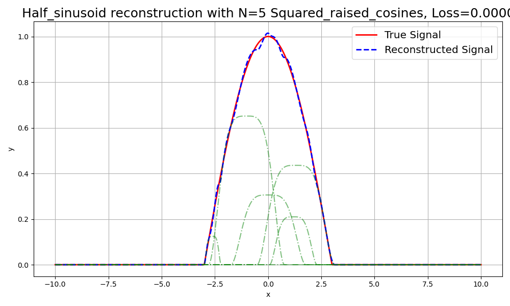
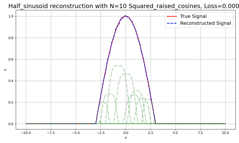
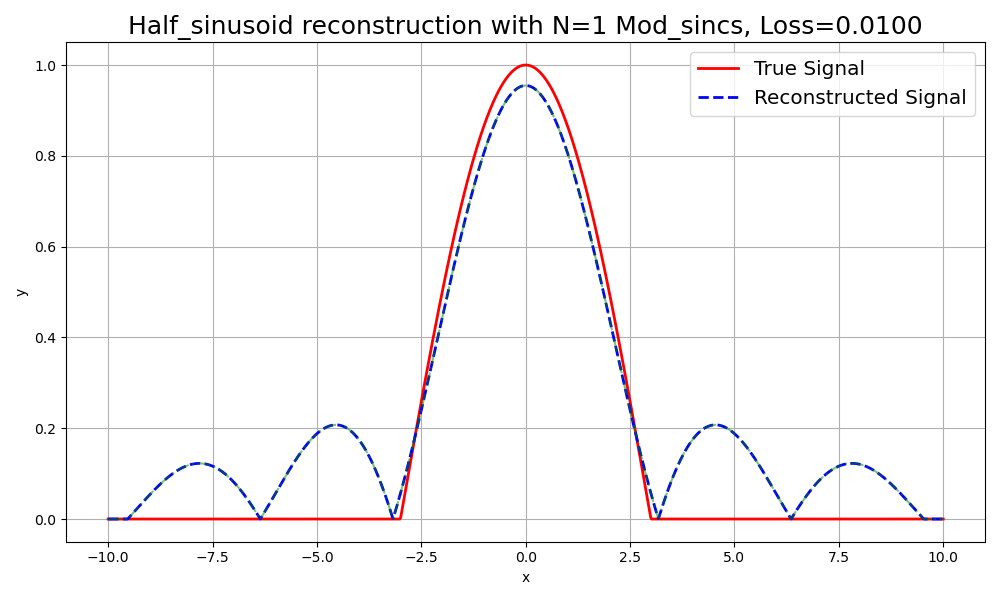
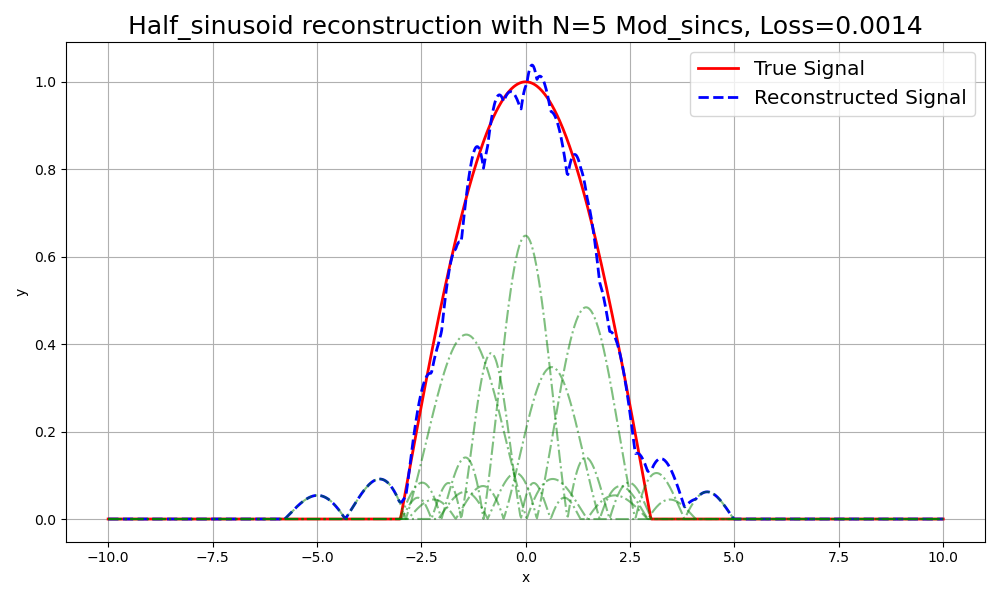
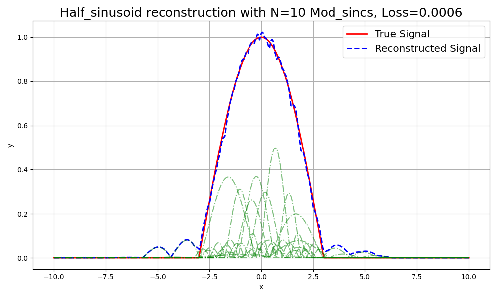
Figure 13: Visualization of 1D simulations for different splatting methods with varying primitives (N=1, N=5, N=10) for a half-sinusoid single pulse. Each row corresponds to a specific splatting method: Gaussian, Cosine, Squared Cosine, Raised Cosine, Squared Raised Cosine, and Modulated Sinc. The columns represent the number of primitives used.

N=1

N=5

N=10

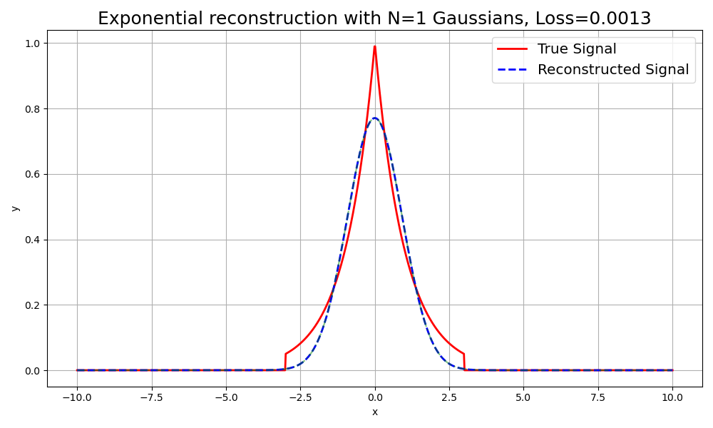
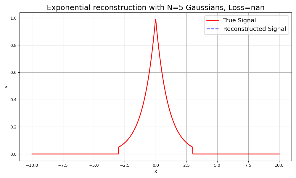
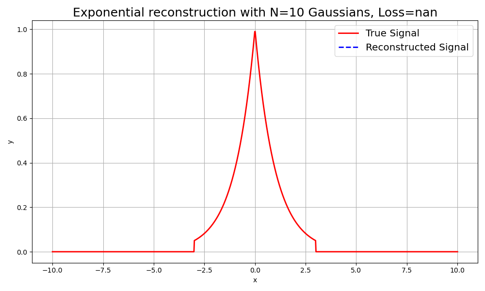
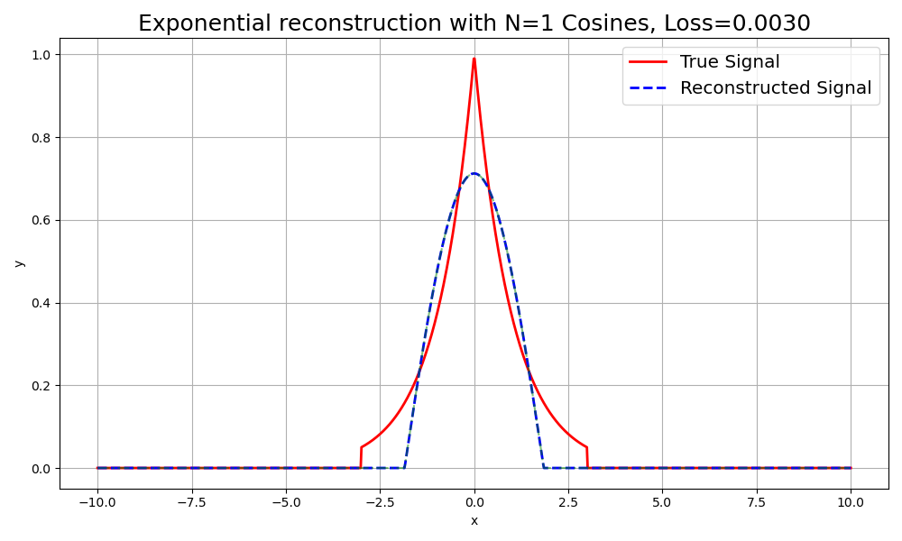
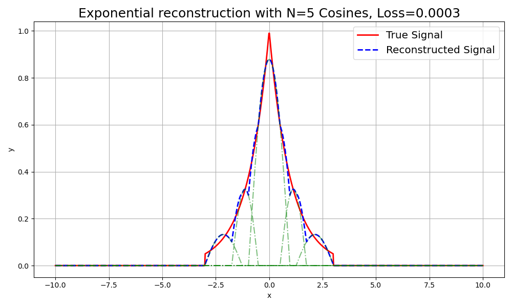
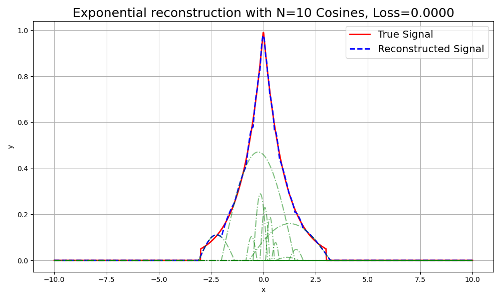
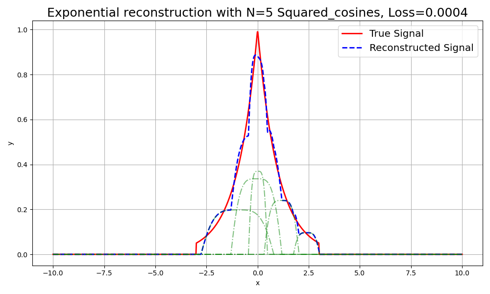
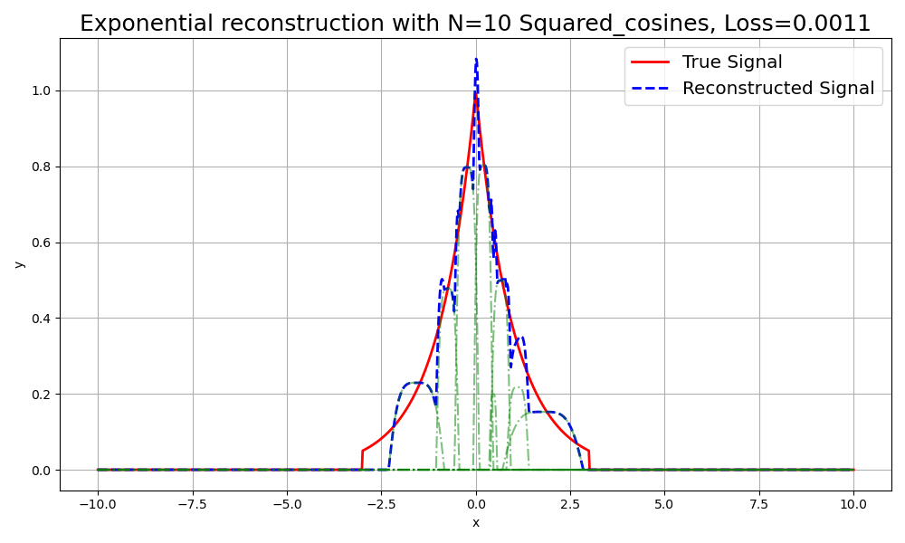
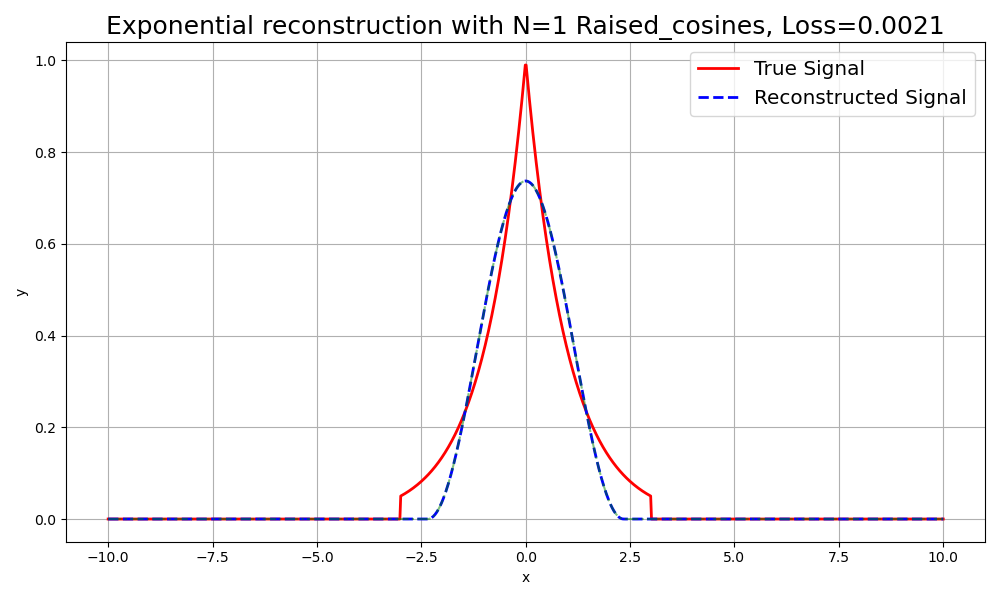
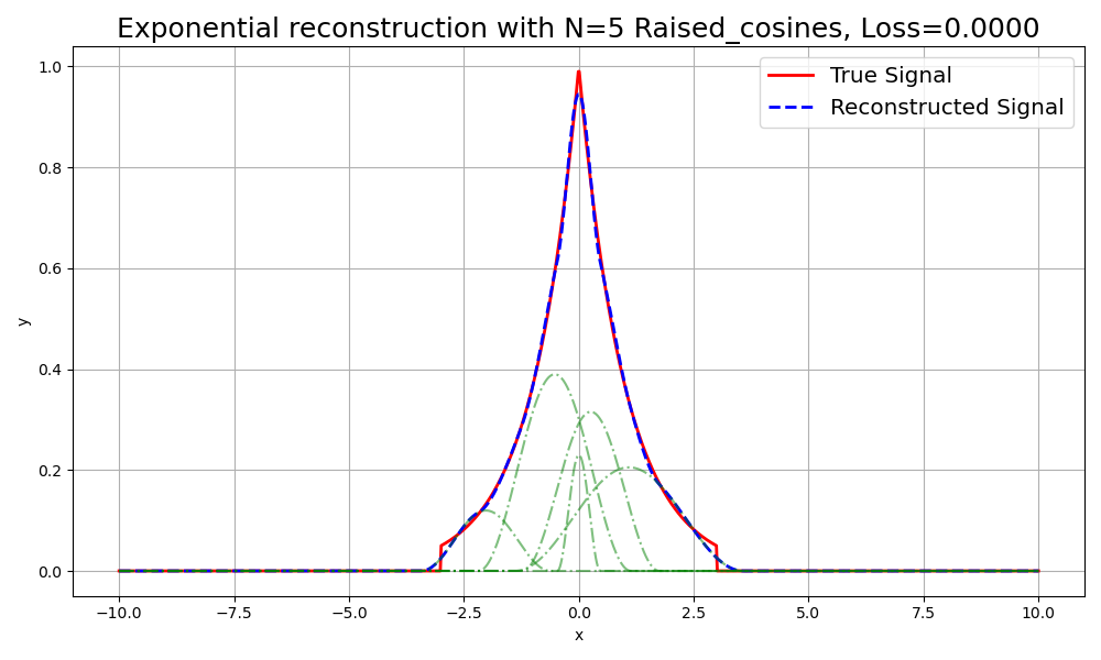
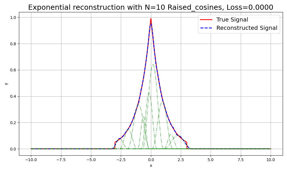
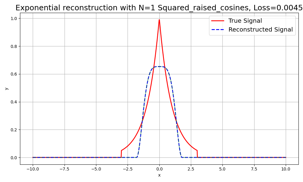
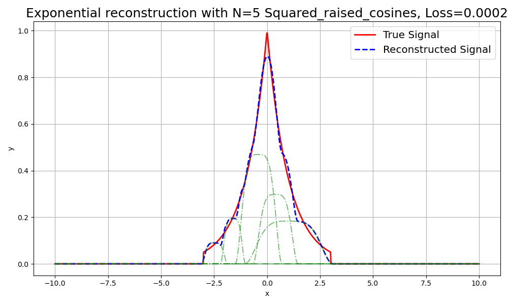
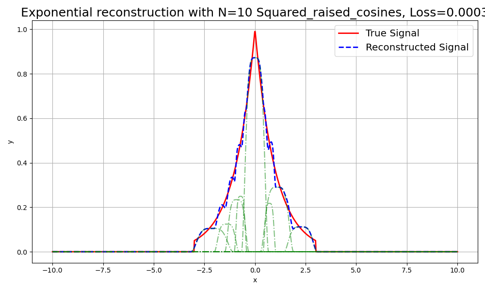
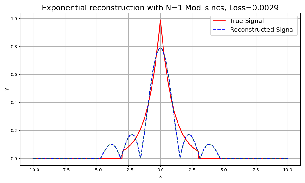
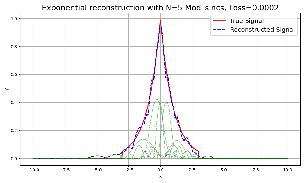
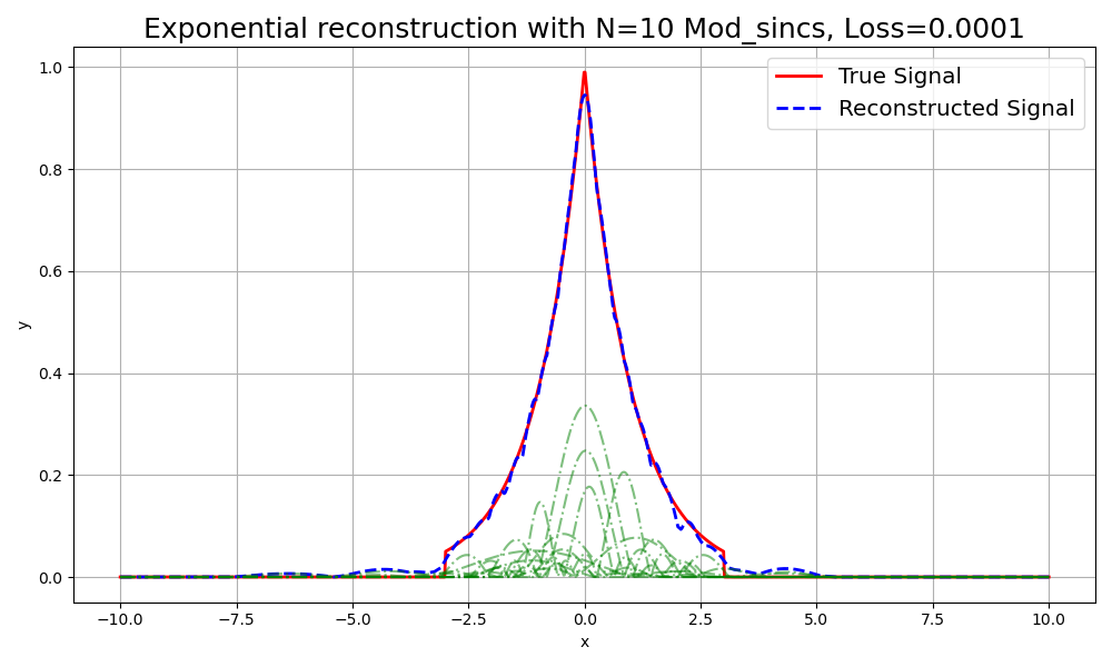
Figure 14: Visualization of 1D simulations for different splatting methods with varying primitives (N=1, N=5, N=10) for a sharp exponential pulse. Each row corresponds to a specific splatting method: Gaussian, Cosine, Squared Cosine, Raised Cosine, Squared Raised Cosine, and Modulated Sinc. The columns represent the number of primitives used.

N=1

N=5

N=10

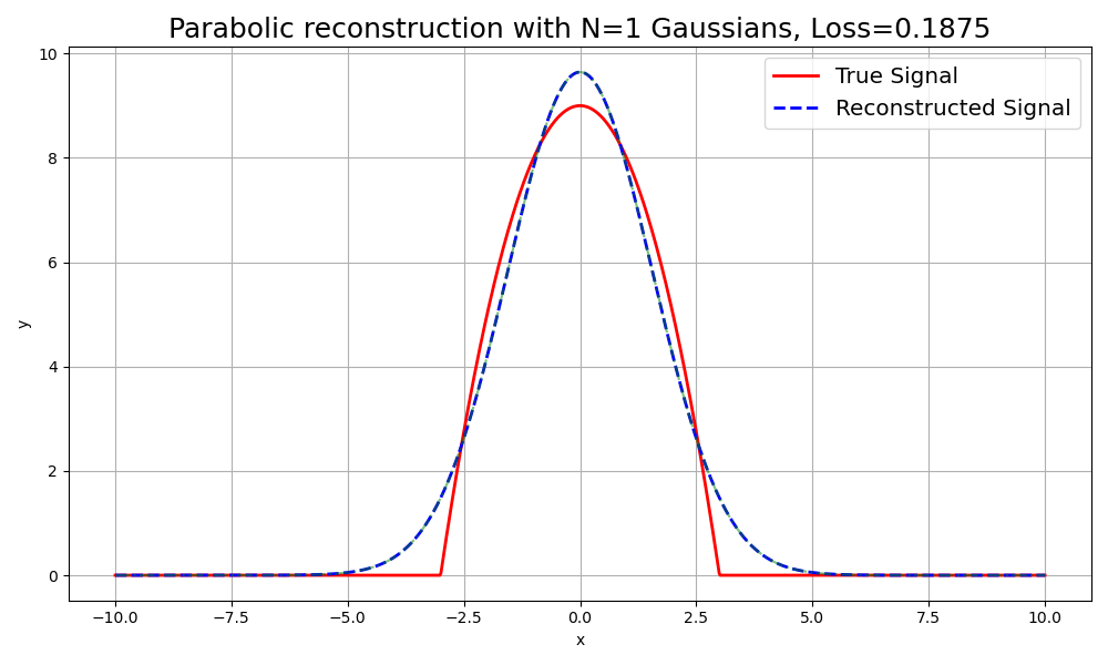
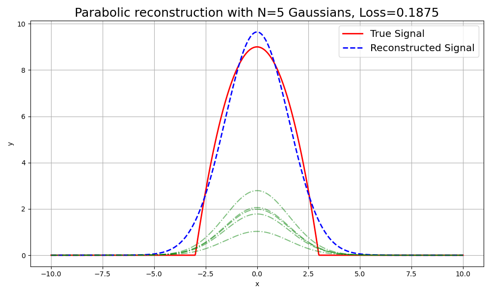
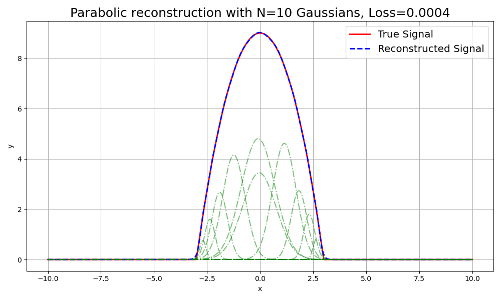
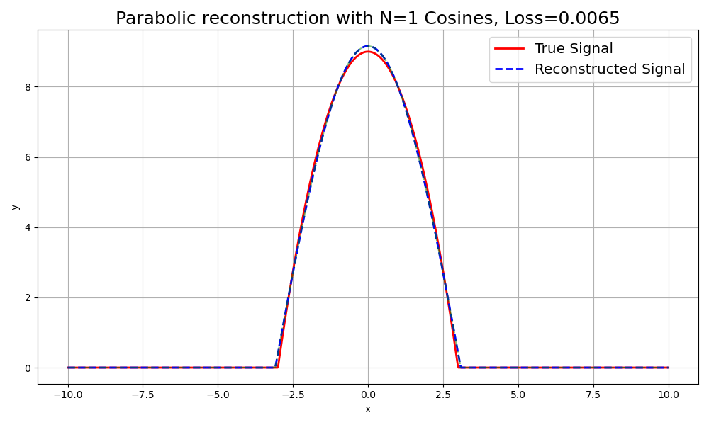
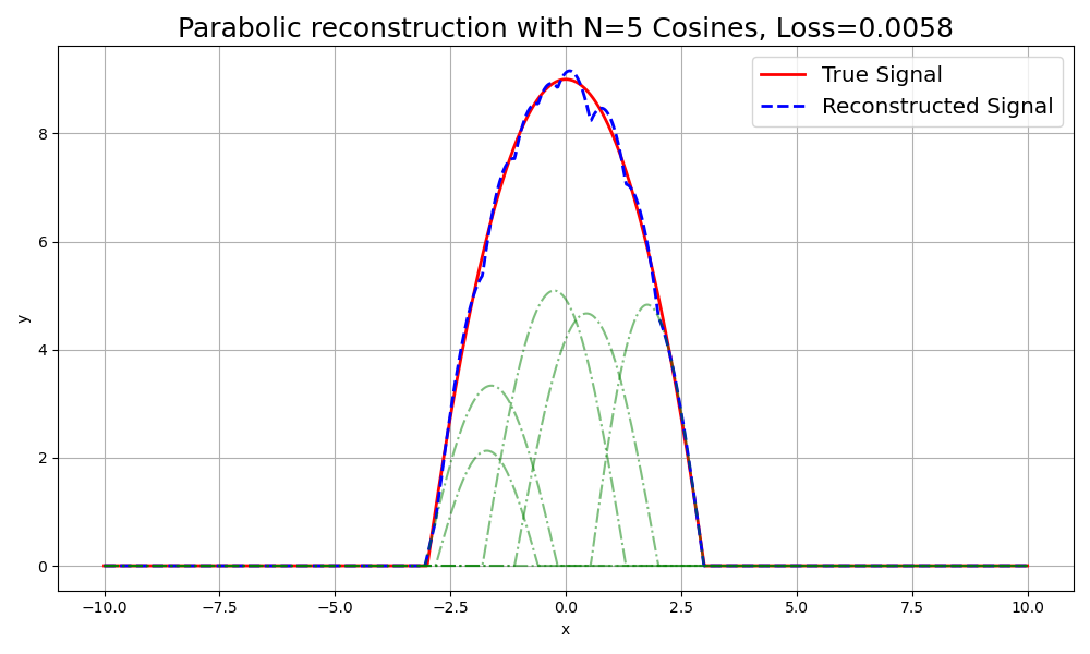
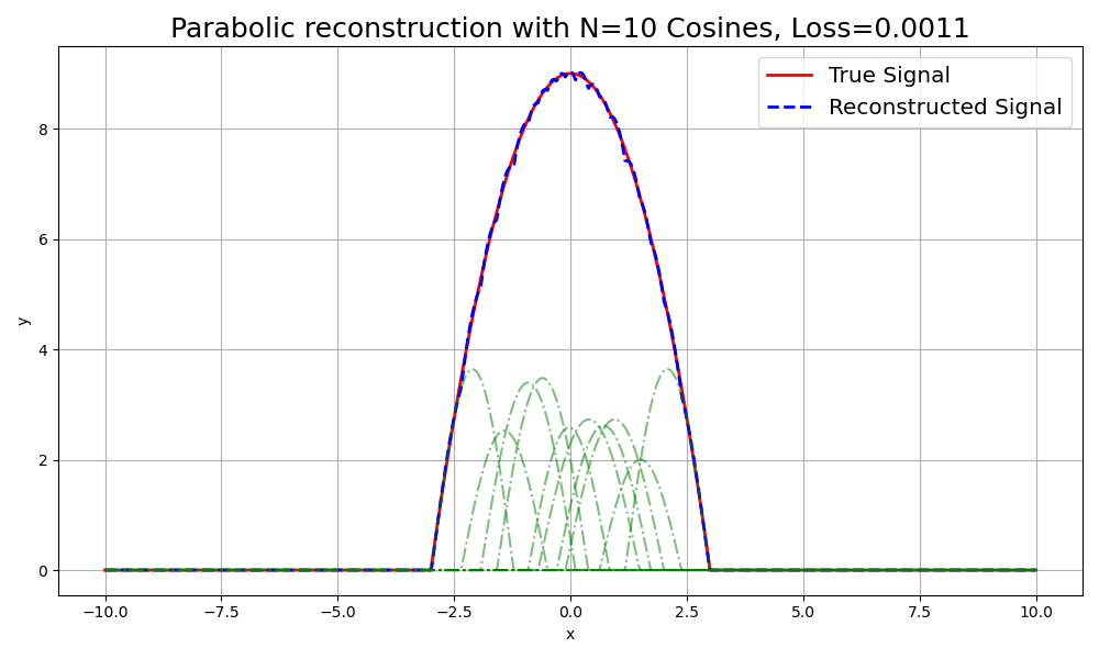
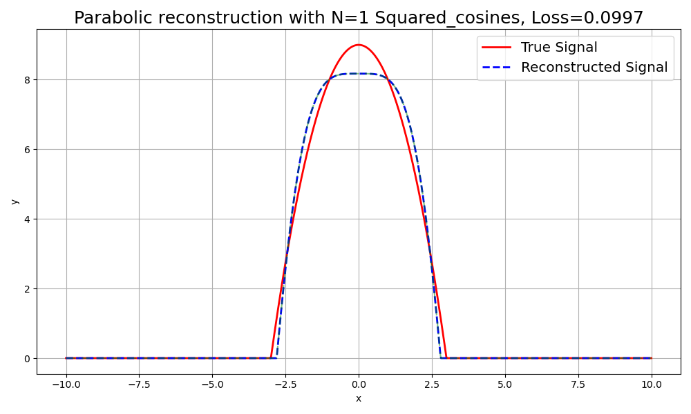
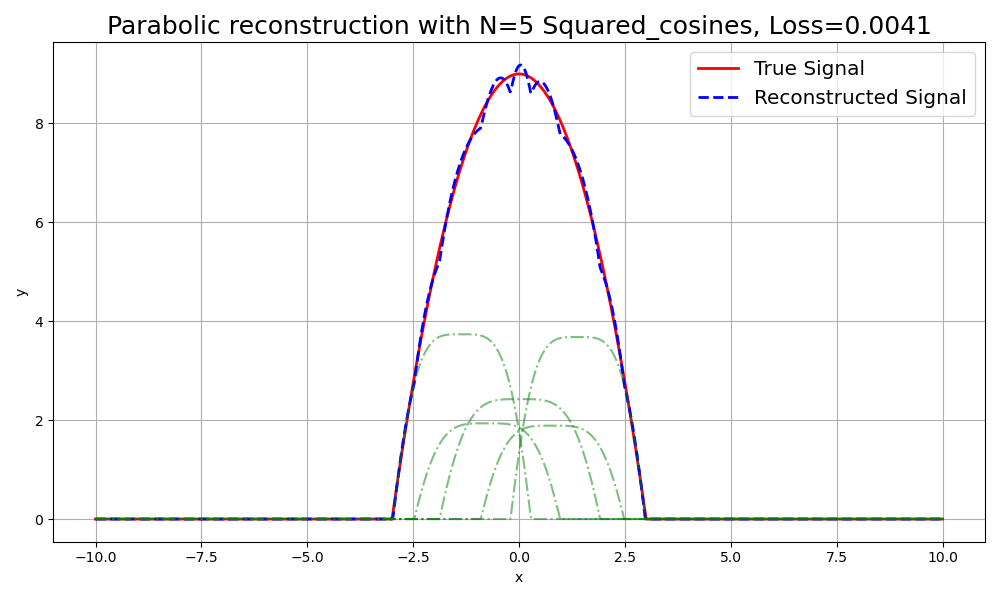
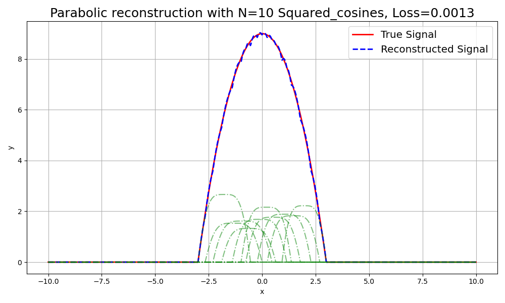
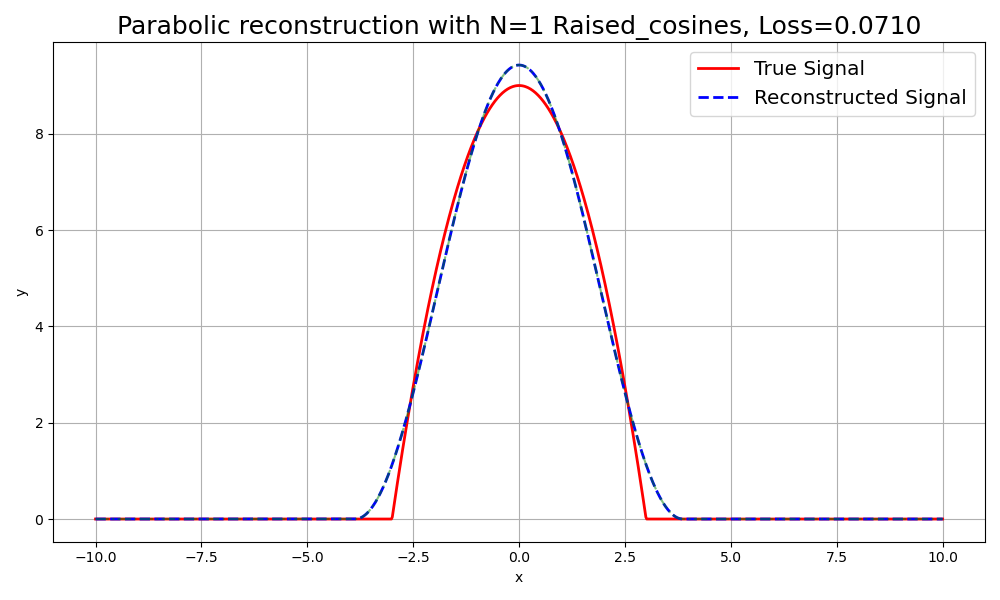
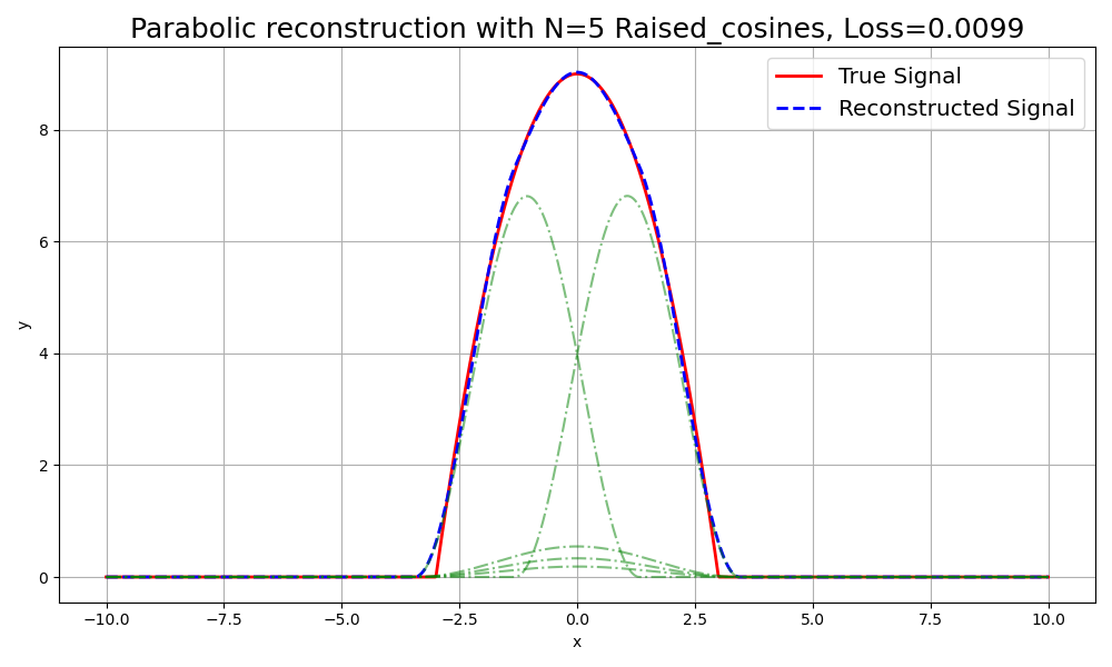
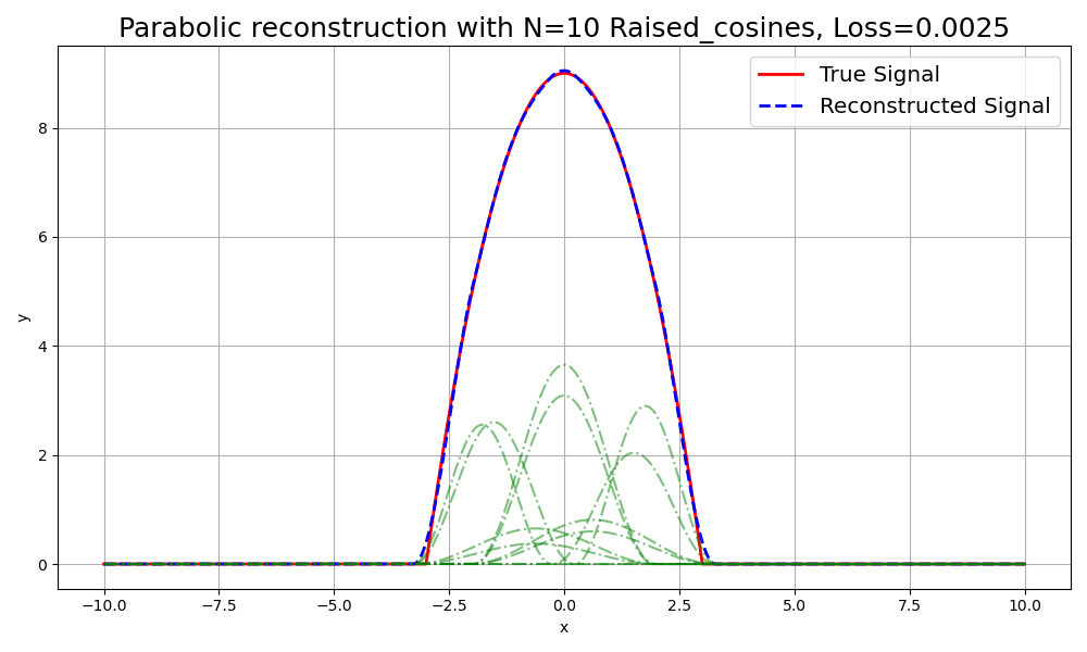
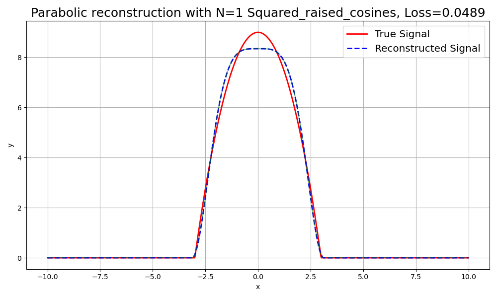
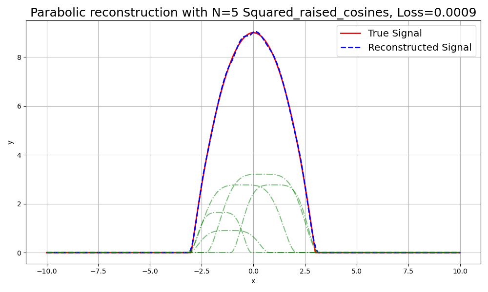
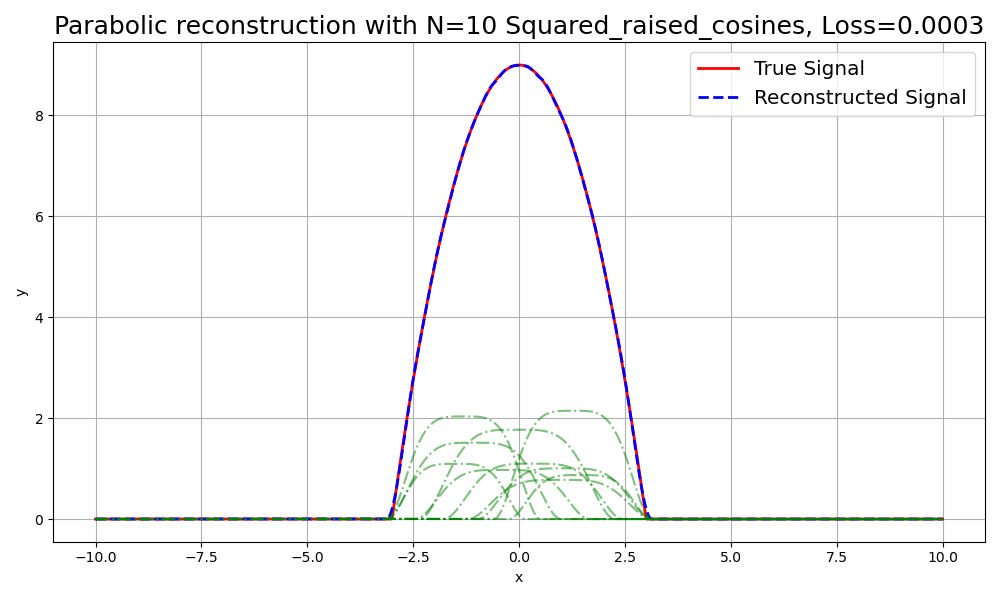
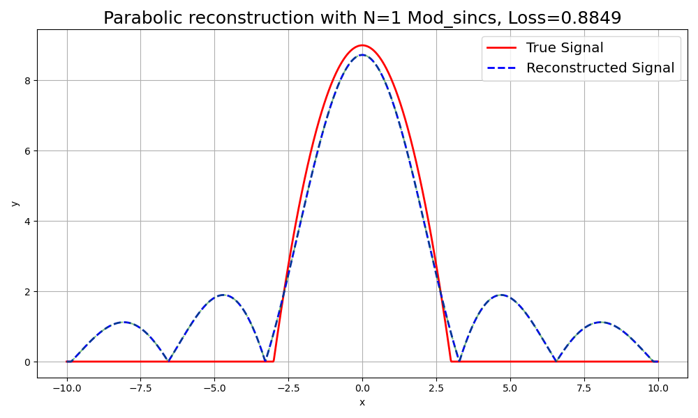
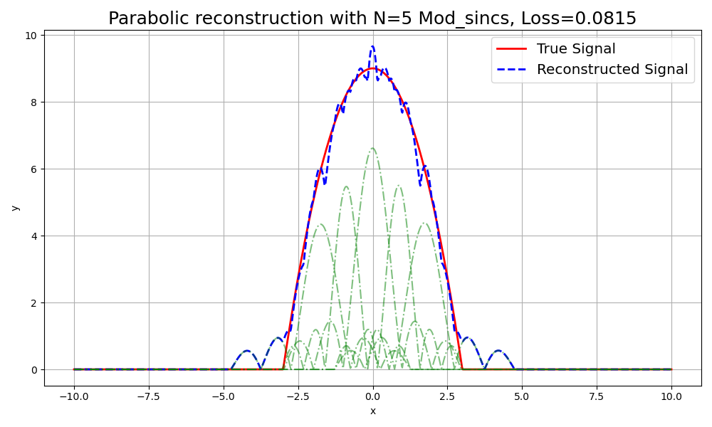
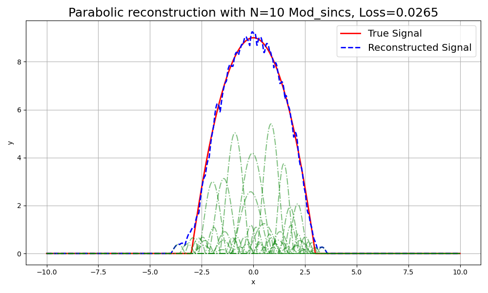
Figure 15: Visualization of 1D simulations for different splatting methods with varying primitives (N=1, N=5, N=10) for a parabolic pulse. Each row corresponds to a specific splatting method: Gaussian, Cosine, Squared Cosine, Raised Cosine, Squared Raised Cosine, and Modulated Sinc. The columns represent the number of primitives used.

N=1

N=5

N=10

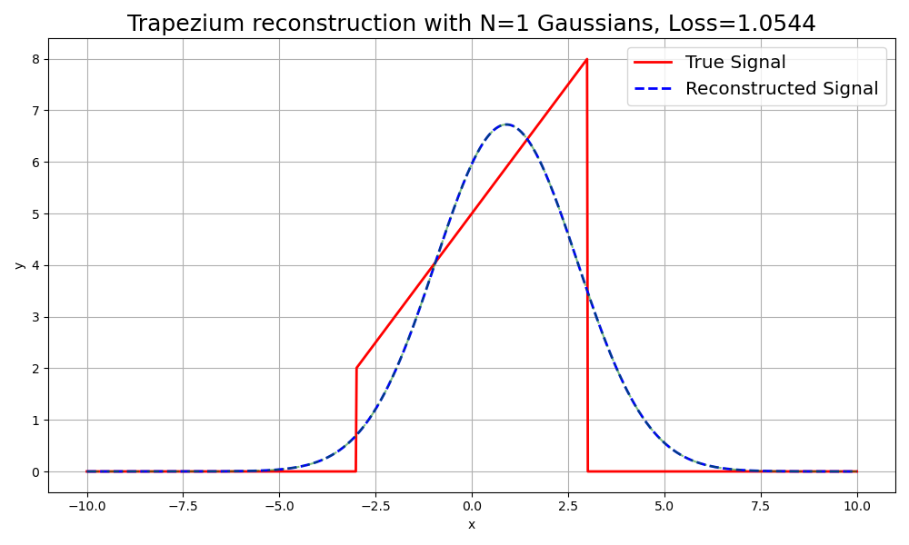
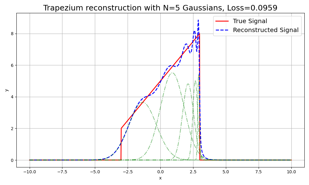
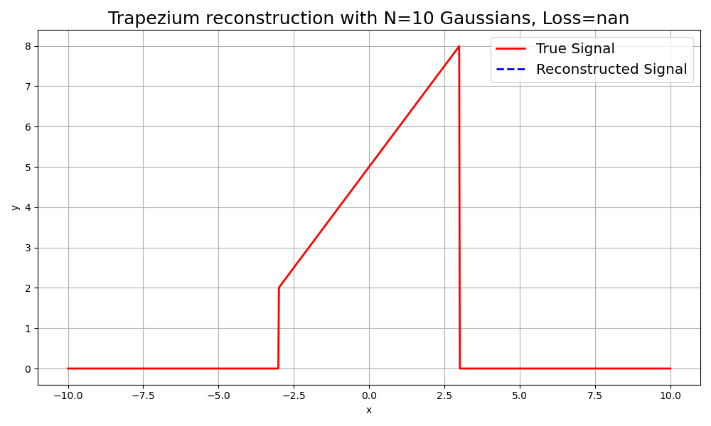
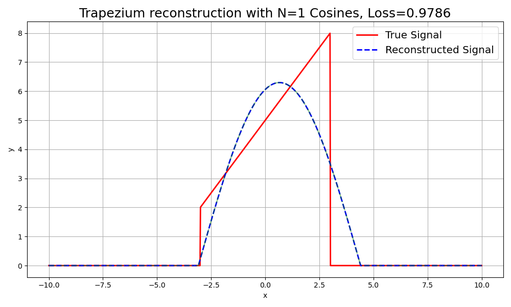
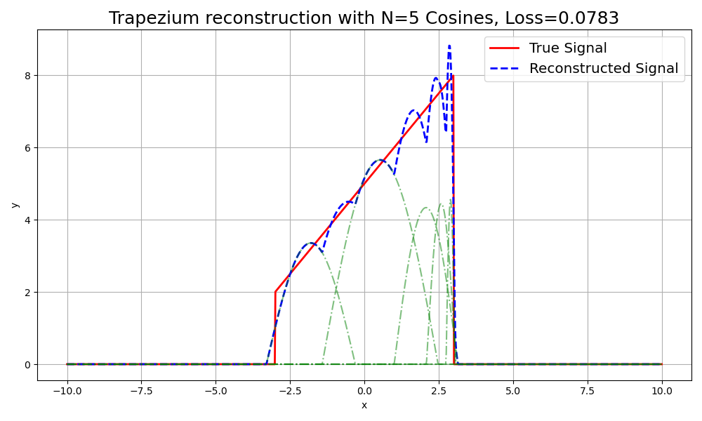
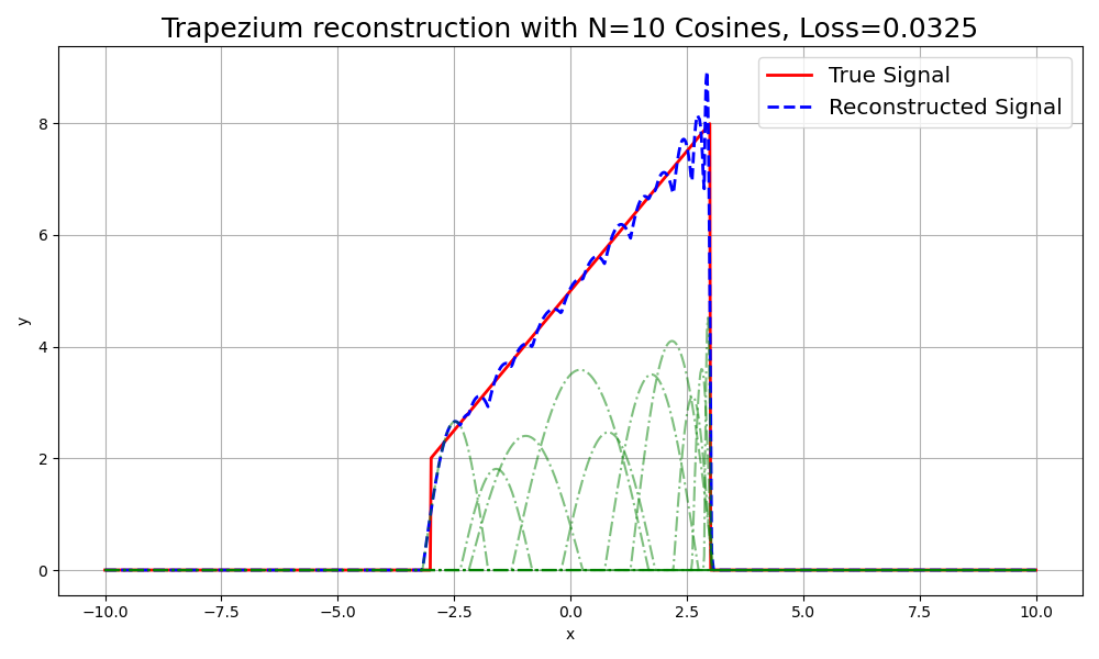
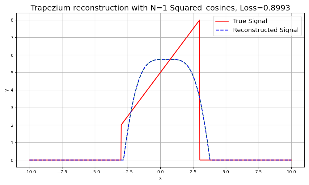
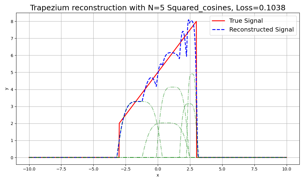
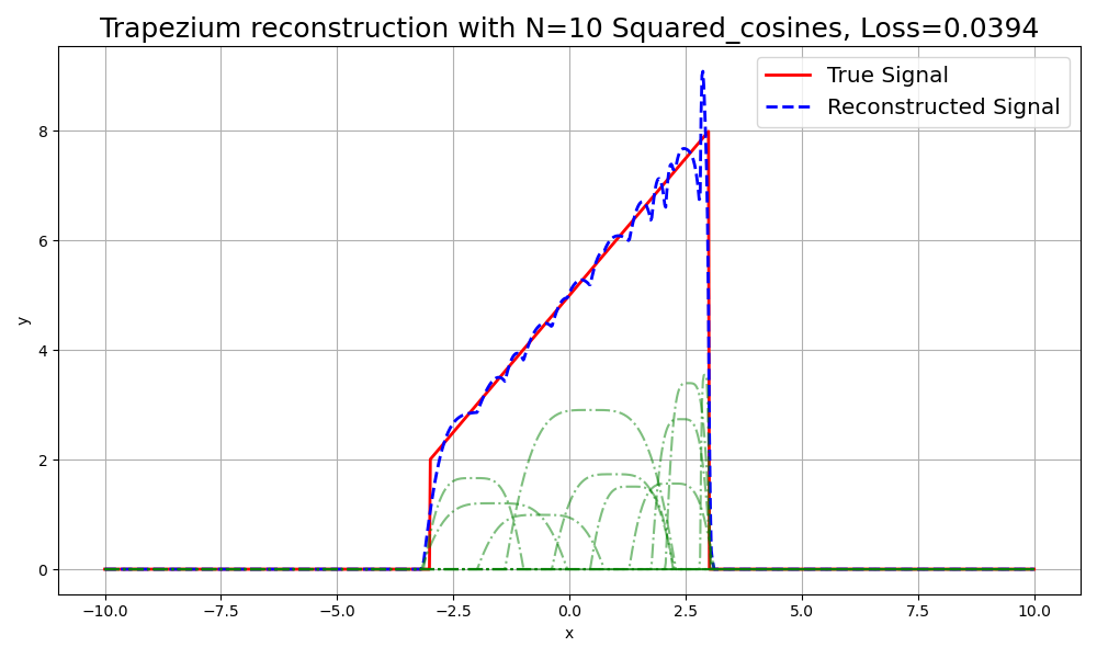
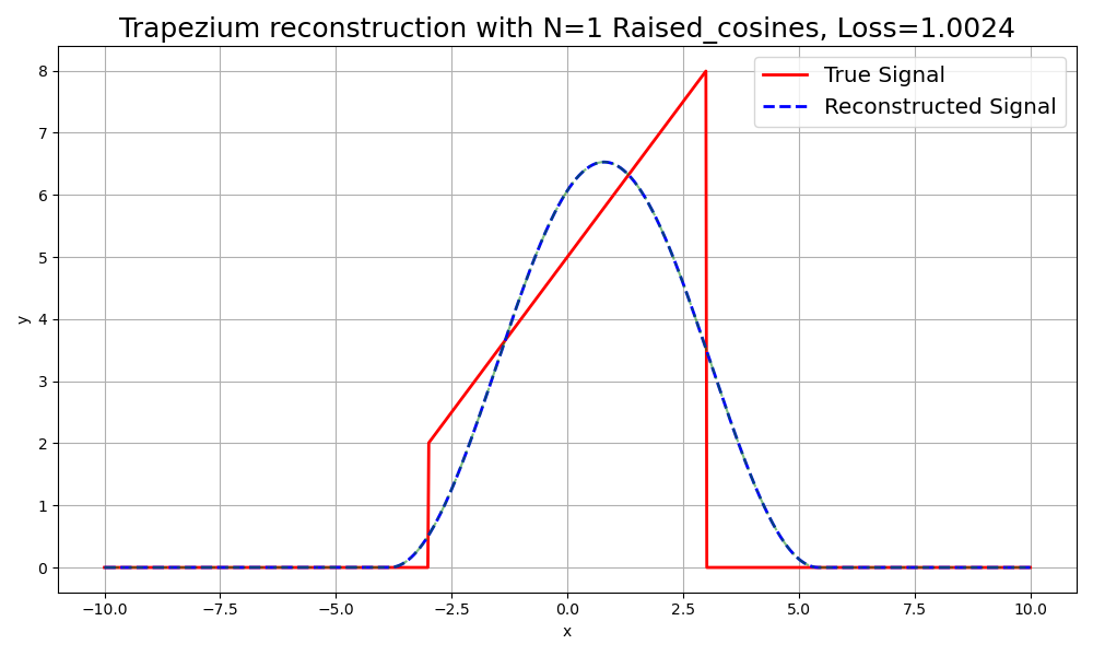
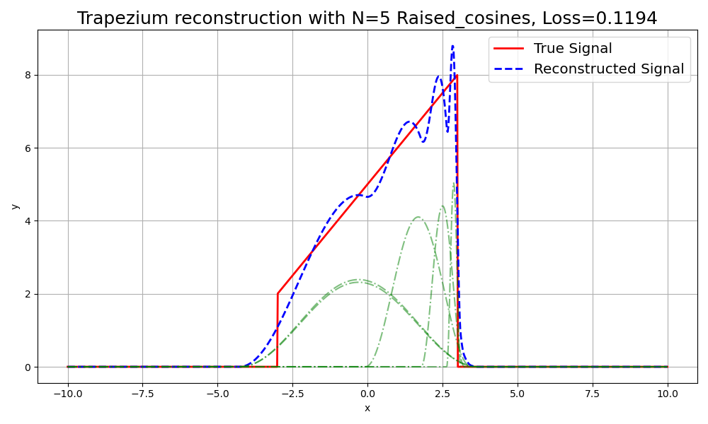
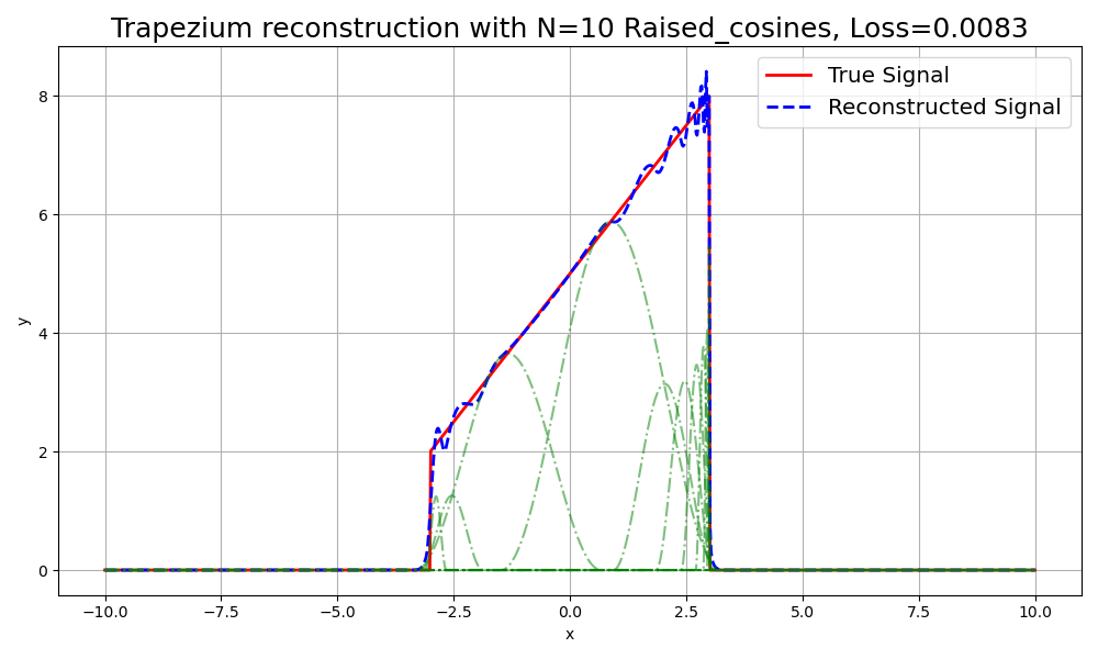
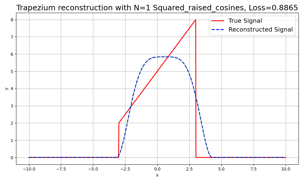
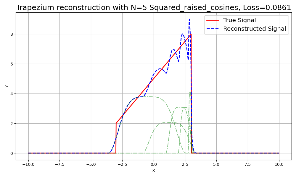
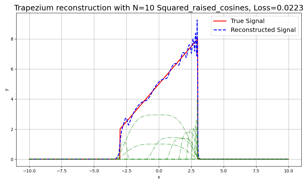
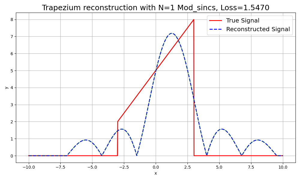
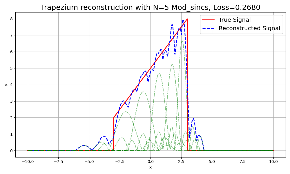
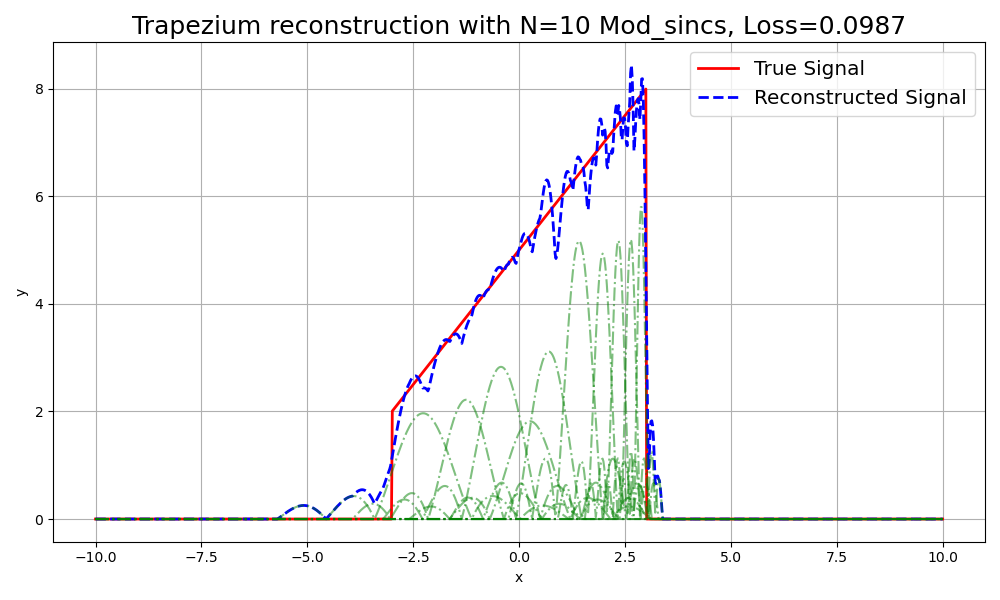
Figure 16: Visualization of 1D simulations for different splatting methods with varying primitives (N=1, N=5, N=10) for a trapezoid pulse. Each row corresponds to a specific splatting method: Gaussian, Cosine, Squared Cosine, Raised Cosine, Squared Raised Cosine, and Modulated Sinc. The columns represent the number of primitives used.

References

- Barron et al. [2021] Jonathan T. Barron, Ben Mildenhall, Matthew Tancik, Peter Hedman, Ricardo Martin-Brualla, and Pratul P. Srinivasan. Mip-nerf: A multiscale representation for anti-aliasing neural radiance fields. In ICCV, pages 5835–5844, 2021.
- Barron et al. [2022] Jonathan T Barron, Ben Mildenhall, Dor Verbin, Pratul P Srinivasan, and Peter Hedman. Mip-nerf 360: Unbounded anti-aliased neural radiance fields. In CVPR, pages 5470–5479, 2022.
- Barron et al. [2023] Jonathan T Barron, Ben Mildenhall, Dor Verbin, Pratul P Srinivasan, and Peter Hedman. Zip-nerf: Anti-aliased grid-based neural radiance fields. In CVPR, pages 19697–19705, 2023.
- Bishop and Nasrabadi [2006] Christopher M Bishop and Nasser M Nasrabadi. Pattern recognition and machine learning. Springer, 2006.
- Casciola et al. [2006] G. Casciola, D. Lazzaro, L.B. Montefusco, and S. Morigi. Shape preserving surface reconstruction using locally anisotropic radial basis function interpolants. Computers & Mathematics with Applications, 51(8):1185–1198, 2006. Radial Basis Functions and Related Multivariate Meshfree Approximation Methods: Theory and Applications.
- Chen et al. [2022] Anpei Chen, Zexiang Xu, Andreas Geiger, Jingyi Yu, and Hao Su. Tensorf: Tensorial radiance fields. In ECCV, pages 333–350. Springer, 2022.
- Chen et al. [2024] Yiwen Chen, Zilong Chen, Chi Zhang, Feng Wang, Xiaofeng Yang, Yikai Wang, Zhongang Cai, Lei Yang, Huaping Liu, and Guosheng Lin. Gaussianeditor: Swift and controllable 3d editing with gaussian splatting. In CVPR, pages 21476–21485, 2024.
- Chen et al. [2025] Yuedong Chen, Haofei Xu, Chuanxia Zheng, Bohan Zhuang, Marc Pollefeys, Andreas Geiger, Tat-Jen Cham, and Jianfei Cai. Mvsplat: Efficient 3D gaussian splatting from sparse multi-view images. In ECCV, pages 370–386, 2025.
- Chung et al. [2023] Jaeyoung Chung, Suyoung Lee, Hyeongjin Nam, Jaerin Lee, and Kyoung Mu Lee. Luciddreamer: Domain-free generation of 3d gaussian splatting scenes, 2023.
- Deng et al. [2022] Kangle Deng, Andrew Liu, Jun-Yan Zhu, and Deva Ramanan. Depth-supervised nerf: Fewer views and faster training for free. In CVPR, pages 12882–12891, 2022.
- Fei et al. [2024] Ben Fei, Jingyi Xu, Rui Zhang, Qingyuan Zhou, Weidong Yang, and Ying He. 3d gaussian splatting as new era: A survey. IEEE Transactions on Visualization and Computer Graphics, 2024.
- Fridovich-Keil et al. [2022] Sara Fridovich-Keil, Alex Yu, Matthew Tancik, Qinhong Chen, Benjamin Recht, and Angjoo Kanazawa. Plenoxels: Radiance fields without neural networks. In CVPR, pages 5501–5510, 2022.
- Garbin et al. [2021] Stephan J Garbin, Marek Kowalski, Matthew Johnson, Jamie Shotton, and Julien Valentin. Fastnerf: High-fidelity neural rendering at 200fps. In ICCV, pages 14346–14355, 2021.
- Gortler et al. [1996] Steven J. Gortler, Radek Grzeszczuk, Richard Szeliski, and Michael F. Cohen. The lumigraph. In Proceedings of the 23rd Annual Conference on Computer Graphics and Interactive Techniques, page 43–54, New York, NY, USA, 1996. Association for Computing Machinery.
- Hamdi et al. [2024] Abdullah Hamdi, Luke Melas-Kyriazi, Jinjie Mai, Guocheng Qian, Ruoshi Liu, Carl Vondrick, Bernard Ghanem, and Andrea Vedaldi. Ges: Generalized exponential splatting for efficient radiance field rendering. In CVPR, pages 19812–19822, 2024.
- Haque et al. [2023] Ayaan Haque, Matthew Tancik, Alexei A Efros, Aleksander Holynski, and Angjoo Kanazawa. Instruct-nerf2nerf: Editing 3d scenes with instructions. In CVPR, pages 19740–19750, 2023.
- Hedman et al. [2018] Peter Hedman, Julien Philip, True Price, Jan-Michael Frahm, George Drettakis, and Gabriel Brostow. Deep blending for free-viewpoint image-based rendering. ACM Transactions on Graphics (Proc. SIGGRAPH Asia), 37(6):257:1–257:15, 2018.
- Hua and Wang [2024] Tongyan Hua and Lin Wang. Benchmarking implicit neural representation and geometric rendering in real-time rgb-d slam. In CVPR, pages 21346–21356, 2024.
- Huang et al. [2024] Jiajun Huang, Hongchuan Yu, Jianjun Zhang, and Hammadi Nait-Charif. Point’n move: Interactive scene object manipulation on gaussian splatting radiance fields. IET Image Processing, 2024.
- Kerbl et al. [2023] Bernhard Kerbl, Georgios Kopanas, Thomas Leimkühler, and George Drettakis. 3d gaussian splatting for real-time radiance field rendering. ACM TOG, 42(4), 2023.
- Khan and Fang [2022] Muhammad Osama Khan and Yi Fang. Implicit neural representations for medical imaging segmentation. In Medical Image Computing and Computer Assisted Intervention – MICCAI 2022, pages 433–443, 2022.
- Knapitsch et al. [2017] Arno Knapitsch, Jaesik Park, Qian-Yi Zhou, and Vladlen Koltun. Tanks and temples: Benchmarking large-scale scene reconstruction. ACM Transactions on Graphics, 36(4), 2017.
- Kratimenos et al. [2025] Agelos Kratimenos, Jiahui Lei, and Kostas Daniilidis. Dynmf: Neural motion factorization for real-time dynamic view synthesis with 3d gaussian splatting. In ECCV, pages 252–269. Springer, 2025.
- Lambda Labs [2024] Lambda Labs. GPU Benchmarks, 2024. Accessed: Nov. 20, 2024.
- Lassner and Zollhöfer [2021] Christoph Lassner and Michael Zollhöfer. Pulsar: Efficient sphere-based neural rendering. In CVPR, 2021.
- Lee et al. [2024] Joo Chan Lee, Daniel Rho, Xiangyu Sun, Jong Hwan Ko, and Eunbyung Park. Compact 3d gaussian representation for radiance field. In CVPR, pages 21719–21728, 2024.
- Lei et al. [2024] Jiahui Lei, Yufu Wang, Georgios Pavlakos, Lingjie Liu, and Kostas Daniilidis. Gart: Gaussian articulated template models. In CVPR, pages 19876–19887, 2024.
- Levoy and Hanrahan [1996] Marc Levoy and Pat Hanrahan. Light field rendering. In Proceedings of the 23rd Annual Conference on Computer Graphics and Interactive Techniques, page 31–42, New York, NY, USA, 1996. Association for Computing Machinery.
- Li et al. [2024] Haolin Li, Jinyang Liu, Mario Sznaier, and Octavia Camps. 3d-hgs: 3d half-gaussian splatting. arXiv preprint arXiv:2406.02720, 2024.
- Lindell et al. [2021] David B Lindell, Julien NP Martel, and Gordon Wetzstein. Autoint: Automatic integration for fast neural volume rendering. In CVPR, pages 14556–14565, 2021.
- Liu et al. [2020] Lingjie Liu, Jiatao Gu, Kyaw Zaw Lin, Tat-Seng Chua, and Christian Theobalt. Neural sparse voxel fields. pages 15651–15663, 2020.
- Liu et al. [2021] Steven Liu, Xiuming Zhang, Zhoutong Zhang, Richard Zhang, Jun-Yan Zhu, and Bryan Russell. Editing conditional radiance fields. In CVPR, pages 5773–5783, 2021.
- Martin-Brualla et al. [2021] Ricardo Martin-Brualla, Noha Radwan, Mehdi S. M. Sajjadi, Jonathan T. Barron, Alexey Dosovitskiy, and Daniel Duckworth. Nerf in the wild: Neural radiance fields for unconstrained photo collections. In CVPR, pages 7210–7219, 2021.
- Mildenhall et al. [2020] Ben Mildenhall, Pratul P. Srinivasan, Matthew Tancik, Jonathan T. Barron, Ravi Ramamoorthi, and Ren Ng. NeRF: Representing scenes as neural radiance fields for view synthesis. In ECCV, 2020.
- Mildenhall et al. [2022] Ben Mildenhall, Peter Hedman, Ricardo Martin-Brualla, Pratul P Srinivasan, and Jonathan T Barron. Nerf in the dark: High dynamic range view synthesis from noisy raw images. In CVPR, pages 16190–16199, 2022.
- Müller et al. [2022] Thomas Müller, Alex Evans, Christoph Schied, and Alexander Keller. Instant neural graphics primitives with a multiresolution hash encoding. ACM TOG, 41(4):1–15, 2022.
- Park et al. [2021a] Keunhong Park, Utkarsh Sinha, Jonathan T Barron, Sofien Bouaziz, Dan B Goldman, Steven M Seitz, and Ricardo Martin-Brualla. Nerfies: Deformable neural radiance fields. In CVPR, pages 5865–5874, 2021a.
- Park et al. [2021b] Keunhong Park, Utkarsh Sinha, Peter Hedman, Jonathan T Barron, Sofien Bouaziz, Dan B Goldman, Ricardo Martin-Brualla, and Steven M Seitz. Hypernerf: A higher-dimensional representation for topologically varying neural radiance fields. arXiv preprint arXiv:2106.13228, 2021b.
- Pumarola et al. [2021] Albert Pumarola, Enric Corona, Gerard Pons-Moll, and Francesc Moreno-Noguer. D-nerf: Neural radiance fields for dynamic scenes. In CVPR, pages 10318–10327, 2021.
- Rebain et al. [2021] Daniel Rebain, Wei Jiang, Soroosh Yazdani, Ke Li, Kwang Moo Yi, and Andrea Tagliasacchi. Derf: Decomposed radiance fields. In CVPR, pages 14153–14161, 2021.
- Reiser et al. [2021] Christian Reiser, Songyou Peng, Yiyi Liao, and Andreas Geiger. Kilonerf: Speeding up neural radiance fields with thousands of tiny mlps. In CVPR, pages 14335–14345, 2021.
- Ren et al. [2024] Jiawei Ren, Liang Pan, Jiaxiang Tang, Chi Zhang, Ang Cao, Gang Zeng, and Ziwei Liu. Dreamgaussian4d: Generative 4d gaussian splatting, 2024.
- Roessle et al. [2022] Barbara Roessle, Jonathan T Barron, Ben Mildenhall, Pratul P Srinivasan, and Matthias Nießner. Dense depth priors for neural radiance fields from sparse input views. In CVPR, pages 12892–12901, 2022.
- Saratchandran et al. [2024] Hemanth Saratchandran, Sameera Ramasinghe, Violetta Shevchenko, Alexander Long, and Simon Lucey. A sampling theory perspective on activations for implicit neural representations, 2024.
- Schonberger and Frahm [2016] Johannes L Schonberger and Jan-Michael Frahm. Structure-from-motion revisited. In CVPR, pages 4104–4113, 2016.
- Schwarz et al. [2020] Katja Schwarz, Yiyi Liao, Michael Niemeyer, and Andreas Geiger. Graf: Generative radiance fields for 3d-aware image synthesis. In NeurIPS, pages 20154–20166, 2020.
- Shao et al. [2023] Ruizhi Shao, Jingxiang Sun, Cheng Peng, Zerong Zheng, Boyao Zhou, Hongwen Zhang, and Yebin Liu. Control4d: Dynamic portrait editing by learning 4d gan from 2d diffusion-based editor. arXiv preprint arXiv:2305.20082, 2(6):16, 2023.
- Shi et al. [2023] Jin-Chuan Shi, Miao Wang, Hao-Bin Duan, and Shao-Hua Guan. Language embedded 3d gaussians for open-vocabulary scene understanding, 2023.
- Skodras et al. [2001] A. Skodras, C. Christopoulos, and T. Ebrahimi. The jpeg 2000 still image compression standard. IEEE Signal Processing Magazine, 18(5):36–58, 2001.
- Snavely et al. [2006] Noah Snavely, Steven M. Seitz, and Richard Szeliski. Photo tourism: exploring photo collections in 3d. ACM Trans. Graph., 25(3):835–846, 2006.
- Su et al. [2022] Kun Su, Mingfei Chen, and Eli Shlizerman. Inras: Implicit neural representation for audio scenes. In NeurIPS, pages 8144–8158, 2022.
- Sun et al. [2022] Jingxiang Sun, Xuan Wang, Yong Zhang, Xiaoyu Li, Qi Zhang, Yebin Liu, and Jue Wang. Fenerf: Face editing in neural radiance fields. In CVPR, pages 7672–7682, 2022.
- Sun et al. [2024] Jiakai Sun, Han Jiao, Guangyuan Li, Zhanjie Zhang, Lei Zhao, and Wei Xing. 3dgstream: On-the-fly training of 3d gaussians for efficient streaming of photo-realistic free-viewpoint videos. In CVPR, pages 20675–20685, 2024.
- Tancik et al. [2022] Matthew Tancik, Vincent Casser, Xinchen Yan, Sabeek Pradhan, Ben Mildenhall, Pratul P Srinivasan, Jonathan T Barron, and Henrik Kretzschmar. Block-nerf: Scalable large scene neural view synthesis. In CVPR, pages 8248–8258, 2022.
- Tang et al. [2024] Jiaxiang Tang, Jiawei Ren, Hang Zhou, Ziwei Liu, and Gang Zeng. Dreamgaussian: Generative gaussian splatting for efficient 3d content creation, 2024.
- Wallace [1992] G.K. Wallace. The jpeg still picture compression standard. IEEE Transactions on Consumer Electronics, 38(1):xviii–xxxiv, 1992.
- Westover [1989] Lee Westover. Interactive volume rendering. In Proceedings of the 1989 Chapel Hill Workshop on Volume Visualization, page 9–16, New York, NY, USA, 1989. Association for Computing Machinery.
- Westover [1990] Lee Westover. Footprint evaluation for volume rendering. In Proceedings of the 17th Annual Conference on Computer Graphics and Interactive Techniques, page 367–376, New York, NY, USA, 1990. Association for Computing Machinery.
- Wu et al. [2024] Guanjun Wu, Taoran Yi, Jiemin Fang, Lingxi Xie, Xiaopeng Zhang, Wei Wei, Wenyu Liu, Qi Tian, and Xinggang Wang. 4d gaussian splatting for real-time dynamic scene rendering. In CVPR, pages 20310–20320, 2024.
- Xie et al. [2024] Tianyi Xie, Zeshun Zong, Yuxing Qiu, Xuan Li, Yutao Feng, Yin Yang, and Chenfanfu Jiang. Physgaussian: Physics-integrated 3d gaussians for generative dynamics. In CVPR, pages 4389–4398, 2024.
- Xu et al. [2022] Qiangeng Xu, Zexiang Xu, Julien Philip, Sai Bi, Zhixin Shu, Kalyan Sunkavalli, and Ulrich Neumann. Point-nerf: Point-based neural radiance fields. In CVPR, pages 5438–5448, 2022.
- Yan et al. [2024] Chi Yan, Delin Qu, Dan Xu, Bin Zhao, Zhigang Wang, Dong Wang, and Xuelong Li. Gs-slam: Dense visual slam with 3d gaussian splatting. In CVPR, pages 19595–19604, 2024.
- Yang et al. [2021] Bangbang Yang, Yinda Zhang, Yinghao Xu, Yijin Li, Han Zhou, Hujun Bao, Guofeng Zhang, and Zhaopeng Cui. Learning object-compositional neural radiance field for editable scene rendering. In CVPR, pages 13779–13788, 2021.
- Ye et al. [2024] Mingqiao Ye, Martin Danelljan, Fisher Yu, and Lei Ke. Gaussian grouping: Segment and edit anything in 3d scenes. In ECCV, 2024.
- Ye and Kanazawa [2023] Vickie Ye and Angjoo Kanazawa. Mathematical supplement for the gsplat library, 2023.
- Yi et al. [2024] Taoran Yi, Jiemin Fang, Junjie Wang, Guanjun Wu, Lingxi Xie, Xiaopeng Zhang, Wenyu Liu, Qi Tian, and Xinggang Wang. Gaussiandreamer: Fast generation from text to 3d gaussians by bridging 2D and 3D diffusion models. In CVPR, pages 6796–6807, 2024.
- Yu et al. [2021] Alex Yu, Ruilong Li, Matthew Tancik, Hao Li, Ren Ng, and Angjoo Kanazawa. Plenoctrees for real-time rendering of neural radiance fields. In CVPR, pages 5752–5761, 2021.
- Yu et al. [2024a] Heng Yu, Joel Julin, Zoltán A. Milacski, Koichiro Niinuma, and László A. Jeni. Cogs: Controllable gaussian splatting. In CVPR, pages 21624–21633, 2024a.
- Yu et al. [2024b] Ruihan Yu, Tianyu Huang, Jingwang Ling, and Feng Xu. 2dgh: 2d gaussian-hermite splatting for high-quality rendering and better geometry reconstruction. arXiv preprint arXiv:2408.16982, 2024b.
- Yu et al. [2024c] Zehao Yu, Anpei Chen, Binbin Huang, Torsten Sattler, and Andreas Geiger. Mip-splatting: Alias-free 3D Gaussian splatting. In CVPR, pages 19447–19456, 2024c.
- Yu et al. [2024d] Zehao Yu, Anpei Chen, Binbin Huang, Torsten Sattler, and Andreas Geiger. Mip-splatting: Alias-free 3d gaussian splatting. In CVPR, pages 19447–19456, 2024d.
- Zhao et al. [2022] Fuqiang Zhao, Wei Yang, Jiakai Zhang, Pei Lin, Yingliang Zhang, Jingyi Yu, and Lan Xu. Humannerf: Efficiently generated human radiance field from sparse inputs. In CVPR, pages 7743–7753, 2022.
- Zwicker et al. [2002] Matthias Zwicker, Hanspeter Pfister, Jeroen van Baar, and Markus Gross. Ewa splatting. IEEE Transactions on Visualization and Computer Graphics, 8(3):223–238, 2002.