Efficient Algorithm for Sparse Fourier Transform
of Generalized $q$-ary Functions

Abstract

Computing the Fourier transform of a $q$-ary function $f:\mathbb{Z}_{q}^{n}\rightarrow\mathbb{R}$, which maps $q$-ary sequences to real numbers, is an important problem in mathematics with wide-ranging applications in biology, signal processing, and machine learning. Previous studies have shown that, under the sparsity assumption, the Fourier transform can be computed efficiently using fast and sample-efficient algorithms. However, in many practical settings, the function is defined over a more general space—the space of generalized $q$-ary sequences $\mathbb{Z}_{q_{1}}\times\mathbb{Z}_{q_{2}}\times\cdots\times\mathbb{Z}_{q_{n}}$—where each $\mathbb{Z}_{q_{i}}$ corresponds to integers modulo $q_{i}$. A naive approach involves setting $q=\max_{i}{q_{i}}$ and treating the function as $q$-ary, which results in heavy computational overheads. Herein, we develop GFast, an algorithm that computes the $S$-sparse Fourier transform of $f$ with a sample complexity of $O(Sn)$, computational complexity of $O(Sn\log N)$, and a failure probability that approaches zero as $N=\prod_{i=1}^{n}q_{i}\rightarrow\infty$ with $S=N^{\delta}$ for some $0\leq\delta<1$. In the presence of noise, we further demonstrate that a robust version of GFast computes the transform with a sample complexity of $O(Sn^{2})$ and computational complexity of $O(Sn^{2}\log N)$ under the same high probability guarantees. Using large-scale synthetic experiments, we demonstrate that GFast computes the sparse Fourier transform of generalized $q$-ary functions using $16\times$ fewer samples and running $8\times$ faster than existing algorithms. In real-world protein fitness datasets, GFast explains the predictive interactions of a neural network with $>25\%$ smaller normalized mean-squared error compared to existing algorithms.

1 Introduction

Fourier analysis of $q$-ary functions, which map discrete sequences with $q$ alphabets to real numbers, plays a pivotal role in modeling and understanding complex systems across disciplines such as biology [1], signal processing [2], and machine learning [3]. Any $q$-ary function $f(\mathbf{m}):\mathbb{Z}_{q}^{n}\rightarrow\mathbb{R}$ can be expressed in terms of its Fourier transform $F[{\bf k}]$ as,

$$f(\mathbf{m})=\sum_{\mathbf{k}\in\mathbb{Z}_{q}^{n}}F[\mathbf{k}]\omega^{\langle\mathbf{m},\mathbf{k}\rangle}\quad\mathbf{m}\in\mathbb{Z}_{q}^{n},$$ (1)

where $\omega\coloneqq e^{\frac{2\pi j}{q}}$, and $\mathbf{m}$ and $\mathbf{k}$ are vectors in the $n$-dimensional ring of integers module $q$, denoted as $\mathbb{Z}_{q}^{n}=\{0,1,\dots,q-1\}^{n}$.

Computing the Fourier transform $F$ of a $q$-ary function $f$ is a challenging problem. Without any assumptions, this requires obtaining $N=q^{n}$ samples from $f$ and paying a computational cost of $O(N\log(N))$ to compute the transform using the seminal fast Fourier transform (FFT) algorithm [4]. This algorithm becomes computationally prohibitive for large $q$ or $n$. Fortunately, in practice, most $q$-ary functions have a sparse Fourier transform, meaning $F$ only has a few non-zero coefficients [5, 6]. The $S$-sparse Fourier transform of a $q$-ary function can be computed using efficient algorithms [7] with a sample complexity of $O(Sn)$, akin to the compressed sensing theory [8, 9, 10], and computational complexity of $O(Sn^{2}\log q)$. This computational advantage of sparse Fourier algorithms, compared to methods such as LASSO [11], has enabled several advances, including scalable methods to identify biological interactions in proteins [6, 12], explain machine learning models [13, 14], and regularize neural networks in the spectral domain [5, 3].

Despite this progress, in many applications, $f$ is defined over the product of spaces comprised of alphabets with different sizes. We call such functions $f:\mathbb{Z}_{q_{1}}\times\mathbb{Z}_{q_{2}}\times\cdots\times\mathbb{Z}_{q_{n}}\rightarrow\mathbb{R}$, which map from the product of spaces with different alphabet sizes to real numbers, generalized $q$-ary functions. For instance, consider a length-$n$ protein sequence, which can be naturally encoded as a $q$-ary sequence in $\mathbb{Z}_{q=20}^{n}$ for 20 amino acids. When predicting the protein’s fitness from the sequence, it is common to assume that only a fraction of the amino acids in each protein site are predictive [15]. In these cases, the protein fitness function is best modeled as a generalized $q$-ary function. As another example, consider interactions between a protein, with an alphabet of $20$ amino acids, and a DNA sequence, with an alphabet of $4$ nucleotides. These interactions can only be defined using generalized $q$-ary functions with $q_{i}\in\{4,20\}$.

The sparse Fourier transform of a generalized $q$-ary function $f$ can be computed naively using existing algorithms by setting $q_{\text{max}}=\max_{i}{q_{i}}$ and treating the underlying function as $q_{\text{max}}$-ary. However, this approach superficially inflates the problem’s dimensionality from $\prod_{i=1}^{n}q_{i}$ to $q_{\text{max}}^{n}$ with no change to the number of non-zero Fourier coefficients $S$, leading to a substantial increase in the sample and computational complexity. For example, modeling protein fitness using a generalized $q$-ary function by focusing on the subset of amino acids predictive of a protein function results in more than two folds reduction in the problem dimensionality, from $q_{\text{max}}^{n=12}=8.9\times 10^{12}$ to $\prod_{i=1}^{n=12}q_{i}=8.6\times 10^{10}$ (for more details see Fig. 3). This effect is exacerbated as $n$ grows, making the computation of an otherwise feasible Fourier transform inaccessible due to sample and computational overheads.

In this paper, we consider the problem of computing the sparse Fourier transform of a generalized $q$-ary function $f$, which can be expressed as:

$$f(\mathbf{m})=\sum_{\mathbf{k}\in\mathbb{Z}_{\mathbf{q}}}F[\mathbf{k}]\prod_{i=1}^{\smash{n}}\omega_{q_{i}}^{m_{i}k_{i}},\quad\mathbf{m}\in\mathbb{Z}_{\mathbf{q}},$$ (2)

where $\mathbf{q}=[q_{1},q_{2},\dots,q_{n}]$, $\mathbb{Z}_{\mathbf{q}}=\mathbb{Z}_{q_{1}}\times\mathbb{Z}_{q_{2}}\times\cdots\times\mathbb{Z}_{q_{n}}$ for brevity, and $\omega_{q_{i}}=e^{\frac{2\pi j}{q_{i}}}$. Equation (2) is a natural generalization of the definition of Fourier transform for $q$-ary functions stated in Equation (1); in particular, with $q_{i}=q,\forall i$ the two formulations become identical. Despite their importance, no efficient algorithm currently exists to compute the sparse Fourier transform of generalized $q$-ary functions.

1.1 Contributions

Herein, we summarize the main contributions of our work:

• We develop GFast, an efficient algorithm that computes the sparse Fourier transform of a generalized $q$-ary function in the noise-less setting with a sample complexity of $O(Sn)$ and computational complexity of $O(Sn\log N)$. We make the GFast software available on our GitHub repository.

• We develop a noise-robust version of GFast, dubbed NR-GFast, that computes the transform in the presence of additive Gaussian noise, with a sample complexity of $O(Sn^{2})$ and computational complexity of $O(Sn^{2}\log N)$.

• We conduct large-scale synthetic experiments and demonstrate that GFast computes the sparse Fourier transform of generalized $q$-ary functions using up to $16\times$ fewer samples and runs up to $8\times$ faster compared to existing algorithms treating the function as $q$-ary, with $q=q_{\text{max}}$.

• We conduct real-world experiments to explain a deep neural network trained to predict protein fluorescence from protein sequence in terms of interactions among its amino acids and demonstrate that, given the same sample budget, NR-GFast achieves >$25\%$ smaller normalized mean-squared error than existing algorithms.

1.2 Related Work

Computing the sparse Fourier transform of signals has a rich history, with much of the focus directed toward developing efficient algorithms for the discrete Fourier transform (DFT) [16, 17, 18, 19, 20, 21]. These algorithms leverage the principle of aliasing, where subsampling a signal in the time domain results in a linear mixing, or sketching, of the Fourier coefficients. Various algorithms have been developed to efficiently sketch (encode) and recover (decode) Fourier coefficients. The FFAST [16, 22] algorithm achieves this by inducing sparse graph alias codes in the DFT domain through a subsampling strategy guided by the Chinese Remainder Theorem (CRT) and employing a belief-propagation decoder  [23, 24] to find the non-zero Fourier coefficients. Inspired by this coding-theoretic framework, efficient algorithms are developed for the problem of computing the sparse Walsh Hadamard transform of pseudo-Boolean functions—a special case of a $q$-ary function with $q=2$ [25, 18, 26, 27]. The recently developed $q$-SFT [7] algorithm computes the sparse Fourier transform of a $q$-ary function for any integer $q$. GFast builds on the coding-theoretic framework in $q$-SFT and develops a new algorithm to compute the sparse Fourier transform of generalized $q$-ary functions.

2 Problem Setup

Consider the generalized $q$-ary function $f({\bf m}):\mathbb{Z}_{\mathbf{q}}\rightarrow\mathbb{R}$ and let $N=\prod_{i=1}^{n}q_{i}$. Our goal is to find the Fourier transform of $f$ defined as,

$$F[\mathbf{k}]=\frac{1}{N}\sum_{\mathbf{m}\in\mathbb{Z}_{\mathbf{q}}}f(\mathbf{m})\prod_{i=1}^{n}\omega_{q_{i}}^{-m_{i}k_{i}},\quad\mathbf{k}\in\mathbb{Z}_{\mathbf{q}},$$ (3)

when $F[{\bf k}]$ is $S$-sparse. To establish theoretical guarantees, we make the following assumptions.

Assumption 1.

Let $\mathcal{S}\coloneqq\text{supp}(F)$ denote the support set of $F$ (i.e., the indices ${\bf k}$ of non-zero Fourier coefficients). We will make the following assumptions:

1. Each element in $\mathcal{S}$ is uniformly distributed and chosen randomly across $\mathbb{Z}_{\mathbf{q}}$.

2. The sparsity $S=|\mathcal{S}|$ is sub-linear in $N$, that is, $S=N^{\delta}$ for some $0\leq\delta<1$.

Assumption 2.

We also assume:

1. The Fourier coefficients $F[\mathbf{k}]$, for all $\mathbf{k}\in\mathcal{S}$, are sampled uniformly from the finite set $\mathcal{X}\coloneqq\{\rho,\rho\phi,\rho\phi^{2},\cdots,\rho\phi^{\kappa-1}\}$, where $\phi=e^{j\frac{2\pi}{\kappa}}$ for a constant phase offset $\kappa$ and strength factor $\rho$.

2. The signal-to-noise ratio (SNR) is written as:

   $$\text{SNR}=\frac{||f||^{2}}{N\sigma^{2}}=\frac{||F||^{2}}{\sigma^{2}}=\frac{S\rho^{2}}{\sigma^{2}},$$

   and is assumed to be a constant.

3. We are given access to noisy samples $f(\mathbf{m})+w(\mathbf{m})$, where $w(\mathbf{m})\sim\mathcal{C}\mathcal{N}(0,\sigma^{2})$ is complex Gaussian noise.

3 GFast: Noiseless

We first analyze the case where samples drawn from $f$ are noiseless (i.e., $\sigma^{2}=0$). Following $q$-SFT, GFast finds the non-zero Fourier coefficients in three steps: 1) Subsampling and aliasing, 2) Bin detection, and 3) Peeling.

3.1 Sampling and Aliasing

GFast strategically aliases $f$ by computing small Fourier transforms using certain subsampling patterns. To do this, we create $C$ subsampling groups, each of size $b<n$, and take subsampled Fourier transforms over these samples. For each subsampling group $c$, we create the subsampling matrix $\mathbf{M}_{c}$ as an $n\times b$ matrix with the partial-identity matrix structure:

$$\mathbf{M}_{c}=[\mathbf{0}_{b\times b(c-1)},\mathbf{I}_{b\times b},\mathbf{0}_{b\times(n-cb)}]^{T}.$$ (4)

For each subsampling group, we denote the length-$b$ vector $\mathbf{b}_{c}$ as a size $b$ subvector of $\mathbf{q}$,

$$\mathbf{b}_{c}\coloneqq\mathbf{M}_{c}^{T}\mathbf{q},$$ (5)

and a set of $P$ offsets $\mathbf{d}_{c,p}\in\mathbb{Z}_{\mathbf{q}}$, where $p\in[P]$. For each $c,p$, the subsampled Fourier coefficients $U_{c,p}[\mathbf{j}]$ indexed by $\mathbf{j}\in\mathbb{Z}_{\mathbf{b}_{c}}$ are written as:

$$U_{c,p}[\mathbf{j}]=\frac{1}{B_{c}}\sum_{\bm{\ell}\in\mathbb{Z}_{\mathbf{b}_{c}}}f(\mathbf{M}_{c}\bm{\ell}+\mathbf{d}_{c,p})\prod_{i=1}^{b}\omega_{(\mathbf{b}_{c})_{i}}^{-j_{i}\ell_{i}},\quad\mathbf{j}\in\mathbb{Z}_{\mathbf{b}_{c}}.$$ (6)

In Section 1 of the Appendix, we show that this equals:

$$U_{c,p}[\mathbf{j}]=\sum_{\mathbf{k}:\text{ }\mathbf{M}_{c}^{T}\mathbf{k}=\mathbf{j}}F[\mathbf{k}]\prod_{i=1}^{n}\omega_{q_{i}}^{(\mathbf{d}_{c,p})_{i}k_{i}},\quad\mathbf{k}\in\mathbb{Z}_{\mathbf{q}}.$$ (7)

Let $\mathbf{s}_{c,\mathbf{k}}\in\mathbb{C}^{P}$ be the vector of offset signatures such that the $p^{\text{th}}$ value in $\mathbf{s}_{c,\mathbf{k}}$ is $\prod_{i=1}^{n}\omega_{q_{i}}^{(\mathbf{d}_{c,p})_{i}k_{i}}$. By grouping the subsampled Fourier coefficients as $\mathbf{U}_{c}[\mathbf{j}]=[U_{c,1}[\mathbf{j}],\ldots,U_{c,P}[\mathbf{j}]]$ with their respective offsets stacked as a matrix $\mathbf{D}_{c}\in\mathbb{Z}_{\mathbf{q}}^{P\times n}$, we rewrite Equation (7) as:

$$\mathbf{U}_{c}[\mathbf{j}]=\sum_{\mathbf{k}:\text{ }\mathbf{M}_{c}^{T}\mathbf{k}=\mathbf{j}}F[\mathbf{k}]\mathbf{s}_{c,\mathbf{k}}.$$ (8)

In the noiseless implementation of GFast, we set $P=n$ and choose $\mathbf{D}_{c}=\mathbf{I}_{n\times n}$.

Algorithm 1 GFast

1:$b,C,P,\{\mathbf{M}_{c}\}_{c\in[C]},\{\mathbf{D}_{c}\}_{c\in[C]},I$

2:$\hat{F}\leftarrow\emptyset$

3:for each $c$ in $C$ do $\triangleright$ Subsampling

4:  for each $p$ in $P$ do

5:   $U_{c,p}[\mathbf{j}]=\frac{1}{B_{c}}\sum_{\bm{\ell}\in\mathbb{Z}_{\mathbf{b}_{c}}}f(\mathbf{M}_{c}\bm{\ell}+\mathbf{d}_{c,p})\prod_{i=1}^{b}\omega_{q_{i}}^{-\mathbf{j}_{i}\bm{\ell}_{i}}$

6:  end for

7:end for

8:$\mathcal{S}=\{(c,\mathbf{j}):\text{Type}(U_{c}{\mathbf{j}})=\mathcal{H}_{s}(\hat{\mathbf{k}},\hat{F}[\hat{\mathbf{k}}])\}$

9:$L=\{(c,\mathbf{j}):\text{Type}(U_{c}{\mathbf{j}})=\mathcal{H}_{m}\}$

10:while $i<I\land(|\mathcal{S}|>0)$ do $\triangleright$ Peeling

11:  for each $c$ in $C$ do

12:   for each $\mathbf{j}$ in $\mathbb{Z}_{\mathbf{b}_{c}}$ do

13:     if $\text{Type}(U_{c}[\mathbf{j}])=\mathcal{H}_{S}(\hat{\mathbf{k}},\hat{F}[\hat{\mathbf{k}}])$ then

14:      $\hat{F}\leftarrow\hat{F}\cup(\hat{\mathbf{k}},\hat{F}[\hat{\mathbf{k}})$

15:      for each $c^{\prime}$ in $C$ do

16:        $\mathbf{j}^{\prime}=\mathbf{M}_{c^{\prime}}^{T}\hat{\mathbf{k}}$

17:        $U_{c^{\prime}}[\mathbf{j^{\prime}}]\leftarrow U_{c^{\prime}}[\mathbf{j^{\prime}}]-\hat{F}[\hat{\mathbf{k}}]\mathbf{s}_{c^{\prime},\hat{\mathbf{k}}}$

18:        Update $\mathcal{S},L$

19:      end for

20:     else

21:      Continue to next $\mathbf{j}$.

22:     end if

23:   end for

24:  end for

25:  $i\leftarrow i+1$

26:end while

27:Return $\hat{F}$

3.2 Bin Detection and Recovery

After aliasing $f$, we use the subsampling groups to recover the original Fourier coefficients. Each $\mathbf{U}_{c}[\mathbf{j}]$ is a linear combination of Fourier coefficients $F[\mathbf{k}]$. The Fourier coefficients are recovered using a bin detection procedure, where the objective is to identify which $\mathbf{U}_{c}[\mathbf{j}]$ contains only one Fourier coefficient. To do this, in addition to the offset matrix $\mathbf{D}_{c}$, we choose a fixed delay $\mathbf{d}_{c,0}=\mathbf{0}_{n}$, where $\mathbf{0}_{n}$ is the vector of all $0$’s of length $n$. This means that $U_{c,0}[\mathbf{j}]=\sum_{\mathbf{k}:\mathbf{M}_{c}^{T}\mathbf{k}=\mathbf{j}}F[\mathbf{k}]$. Using $U_{c,0}[\mathbf{j}]$, we are able to identify $\mathbf{U}_{c}[\mathbf{j}]$ as a zero-ton, singleton, or multi-ton bin based on the following criteria:

• Zero-ton verification: $\mathbf{U}_{c}[\mathbf{j}]$ is a zero-ton (denoted by $\mathcal{H}_{Z}$) if $F[\mathbf{k}]=0$ such that $\mathbf{M}_{c}^{T}\mathbf{k}=\mathbf{j}$ (the summation condition in Equation (8)). In the presence of no noise, this is true when $U_{c,p}[\mathbf{j}]=0$ for all $p=1,\ldots,P$.

• Singleton verification: $\mathbf{U}_{c}[\mathbf{j}]$ is a singleton (denoted by $\mathcal{H}_{S}$) if there exists only one $\mathbf{k}$ where $F[\mathbf{k}]\neq 0$ such that $\mathbf{M}_{c}^{T}\mathbf{k}=\mathbf{j}$. This implies that $|U_{c,1}[\mathbf{j}]|=|U_{c,2}[\mathbf{j}]|=\ldots=|U_{c,P}[\mathbf{j}]|$, meaning that in the noiseless case, $\mathbf{U}_{c}[\mathbf{j}]$ is a singleton if:

  $$\left|\frac{U_{c,p}[\mathbf{j}]}{U_{c,0}[\mathbf{j}]}\right|=1,\quad p=1,2,\ldots,P.$$

• Multi-ton verification: $\mathbf{U}_{c}[\mathbf{j}]$ is a multi-ton (denoted by $\mathcal{H}_{M}$) if there exists more than one $\mathbf{k}$ where $F[\mathbf{k}]\neq 0$ such that $\mathbf{M}_{c}^{T}\mathbf{k}=\mathbf{j}$. In the noiseless case, this means that the following condition is met:

  $$\left|\frac{U_{c,p}[\mathbf{j}]}{U_{c,0}[\mathbf{j}]}\right|\neq 1,\quad p=1,2,\ldots,P.$$

With this, we define the function $\text{Type}(\mathbf{U}_{c}[\mathbf{j}])\rightarrow\{\mathcal{H}_{Z},\mathcal{H}_{M},\mathcal{H}_{S}(\mathbf{k},F[\mathbf{k}])\}$, which, given a bin, returns the type, along with a tuple of $(\mathbf{k},F[\mathbf{k}])$ if the bin is a singleton. If a singleton is found, $U_{c,0}[\mathbf{j}]=F[\mathbf{k}]$. This enables us to use the identity structure of $\mathbf{D}_{c}$ to solve for $\mathbf{k}$:

$$\begin{bmatrix}\text{arg}_{q_{1}}[U_{c,1}[\mathbf{j}]/U_{c,0}[\mathbf{j}]]\\ \vdots\\ \text{arg}_{q_{n}}[U_{c,P}[\mathbf{j}]/U_{c,0}[\mathbf{j}]]\end{bmatrix}=\mathbf{D}_{c}\mathbf{k},$$ (9)

where $\text{arg}_{q_{i}}\colon\mathbb{C}\rightarrow\mathbb{Z}_{q_{i}}$ is the $q_{i}$-quantization of the argument of a complex number defined as,

$$\text{arg}_{q_{i}}(z):=\left\lfloor\frac{q_{i}}{2\pi}\text{arg}(ze^{\frac{j\pi}{q_{i}}})\right\rfloor.$$ (10)

Intuitively, $\text{arg}_{q_{i}}(z)$ discretizes the angle shift between the unshifted coefficient $U_{c,0}[\mathbf{j}]$ and the aliased coefficient $U_{c,i}[\mathbf{j}]$. After obtaining the unknown vector $\mathbf{k}$, the value of $F[\mathbf{k}]$ is directly obtained as $F[\mathbf{k}]=U_{c,0}[\mathbf{j}]$.

3.3 Peeling Decoder

Upon determining the bin type, the final step uses a peeling decoder to identify more singleton bins. This problem is modeled with a bipartite graph, where each $F[\mathbf{k}]$ is a variable node, each $\mathbf{U}_{c}[\mathbf{j}]$ is a check node, and there is an edge between $F[\mathbf{k}]$ and $\mathbf{U}_{c}[\mathbf{j}]$ when $\mathbf{M}_{c}^{T}\mathbf{k}=\mathbf{j}$. The graph is a left-$C$ regular sparse bipartite graph with a total of $SC$ nodes. Fig. 1 shows an illustration of one such bipartite graph. The peeling algorithm is detailed in Algorithm 1. Upon identifying a singleton, for every subsampling group $c$ in $C$, we subtract $F[\mathbf{\mathbf{k}}]$ from every $\mathbf{U}_{c}[\mathbf{M}_{c}^{T}\mathbf{k}]$. This is equivalent to peeling an edge off the bipartite graph. After looping through all subsampled Fourier coefficients, this procedure is repeated until no more singletons can be peeled. Under Assumptions 1 and 2, we prove the following Theorem:

Theorem 1.

Given a function $f$ as Equation (2) that satisfies Assumptions 1 and 2, with each $B_{c}=O(S)$, $C=O(1)$, $P=n$, and $\mathbf{D}_{c}=\mathbf{I}_{n\times n}$, GFast recovers all Fourier coefficients in $\text{supp}(F)$ with probability at least $1-O(1/S)$ with a sample complexity of $O(Sn)$ and computational complexity of $O(Sn\log N)$ using subsampling matrices $\mathbf{M}_{c}$ in Equation (4).

Proof.

The proof is outlined in Section 2 of the Appendix. ∎

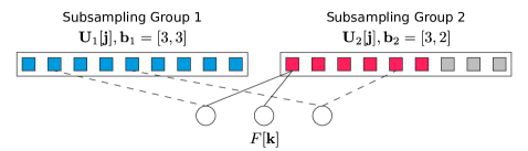
Figure 1: An example of a bipartite graph for computing the sparse Fourier transform of a generalized $q$-ary function with $n=4$, $b=2$, and $\mathbf{q}=[3,3,3,2]$, where $\mathbf{b}_{1}=[3,3]$ (blue squares) and $\mathbf{b}_{2}=[3,2]$ (red squares). Dashed lines represent edges that are peeled in the first iteration of decoding in GFast. Existing algorithms for $q$-ary functions use the $\mathbf{b}_{2}=[3,3]$ (red and gray squares) grouping, which inflates the dimension.

4 GFast: Noise Robust

We develop a version of GFast that accounts for the presence of noise, where $\sigma^{2}>0$, dubbed NR-GFast. Instead of constraining $P=n$ and $\mathbf{D}_{c}=\mathbf{I}_{n\times n}$, given the hyperparameter $P_{1}$, we let $P=P_{1}n$ and $\mathbf{D}_{c}$ be a random matrix in $\mathbb{Z}_{\mathbf{q}}^{P\times n}$. For simplicity, we drop the subsampling group index $c$ and index $\mathbf{j}$ from $\mathbf{U}_{c}[\mathbf{j}]$ and write $\mathbf{U}=[\mathbf{U}_{1},\cdots\mathbf{U}_{p}]^{T}$. For each group, let $\mathbf{S}=[\cdots\mathbf{s_{k}}\cdots]\in\mathbb{C}^{P\times N}$ be the matrix of offset signatures. In the presence of noise, $\mathbf{U}=\mathbf{S}\bm{\alpha}+\mathbf{W}$, where $\bm{\alpha}[\mathbf{k}]=F[\mathbf{k}]$ if $\mathbf{M}^{T}{\mathbf{k}}=\mathbf{j}$, otherwise $\bm{\alpha}[\mathbf{k}]=0$. $\mathbf{W}$ is a matrix of complex multivariate Gaussian noise with zero mean and covariance $\nu_{c}^{2}\mathbf{I}$, such that $\nu_{c}^{2}=\sigma^{2}/B_{c}$.

NR-GFast uses random offsets that individually recover each $\mathbf{k}$ index based on repetition coding. Given a set of $P_{1}$ random offsets $\mathbf{d}_{p\in[P_{1}]}$ such that $P=P_{1}n$, we modulate each offset with each column of the identity matrix such that we have $n$ offsets $\mathbf{d}_{p,r}:$

$$\mathbf{d}_{p,r}=\mathbf{d}_{p}\oplus_{q}\mathbf{e}_{r},\forall p\in[P_{1}],\quad\forall r\in n.$$ (11)

This generates $C$ matrices $\mathbf{D_{c}}\in\mathbb{Z}_{\textbf{q}}^{P\times n}$. We then use a majority test to estimate the $r^{\text{th}}$ value of $\hat{\mathbf{k}}$, where $\hat{\mathbf{k}}$ is the estimated index of $\mathbf{k}$:

$$\hat{k}_{r}=\operatorname*{arg\,max}_{a\in\mathbb{Z}_{q_{r}}}\sum_{p\in[P_{1}]}\mathbbm{1}\{a=\text{arg}_{q_{r}}[U_{p,r}/U_{p}]\},$$ (12)

where $\mathbbm{1}$ denotes the indicator function, and $\hat{k}_{r}$ denotes the value $a\leq q_{r}$ that is the maximum likelihood estimate of $q_{r}$. Then, for some $\gamma\in(0,1)$, bin detection is modified using the following criteria:

• Zero-ton verification: $\text{Type}(\mathbf{U}_{c}[\mathbf{j}])=\mathcal{H}_{Z}$ if $\frac{1}{P}\|\mathbf{U}_{c}[\mathbf{j}]\|^{2}\leq(1+\gamma)\nu_{c}^{2}$.

• Singleton verification: After ruling out zero-tons, we estimate $(\hat{\mathbf{k}},\hat{F}[\hat{\mathbf{k}}])$, where $\hat{F}[\hat{\mathbf{k}}]$ is the estimated Fourier coefficient corresponding to $\hat{\mathbf{k}}$, using the procedure described in the noiseless case. We verify if $\mathbf{U}_{c}[\mathbf{j}]$ is a singleton if $\frac{1}{P}\|\mathbf{U}_{c}[\mathbf{j}]-\hat{F}[\hat{\mathbf{k}}]\mathbf{s}_{c,\hat{\mathbf{k}}}\|^{2}\leq(1+\gamma)\nu_{c}^{2}$.

• Multi-ton verification: If neither $\text{Type}(\mathbf{U}_{c}[\mathbf{j}])=\mathcal{H}_{Z}$ nor $\text{Type}(\mathbf{U}_{c}[\mathbf{j}])=\mathcal{H}_{S}$, then $\text{Type}(\mathbf{U}_{c}[\mathbf{j}])=\mathcal{H}_{M}$.

Using the above setup, the random offsets satisfy the following proposition:

Proposition 1.

Given a singleton bin $(\mathbf{k},F[\mathbf{k}])$, the $q_{r}$-quantized ratio as defined in Equation (10) for

$$U_{p} =F[\mathbf{k}]\prod_{i=1}^{n}\omega_{q_{i}}^{(\mathbf{d}_{p})_{i}k_{i}}+W_{p},$$ (13)

$$U_{p,r} =F[\mathbf{k}]\prod_{i=1}^{n}\omega_{q_{i}}^{(\mathbf{d}_{p,r})_{i}k_{i}}+W_{p,r},$$

satisfies $\text{arg}_{q_{r}}[U_{p,r}/U_{p}]=\langle\mathbf{e}_{r},\mathbf{k}\rangle\otimes_{q_{r}}Z_{p,r}$, where $Z_{p,r}$ is a random variable over $\mathbb{Z}_{q_{r}}$ with a probability $p_{i}\coloneqq\mathbb{P}(Z_{p,r}=i)$. Let $\sum_{i\neq 0}p_{i}\coloneqq\mathbb{P}_{e}$. $\mathbb{P}_{e}$ is upper bounded by $2e^{-\frac{\zeta}{2}\text{SNR}}$ for $\zeta=\eta_{c}\sin^{2}(\pi/2q_{r})$.

Proof.

The proof is outlined in Section 3 of the Appendix. ∎

Using Proposition 1, we prove the following Theorem:

Theorem 2.

Given a function $f$ as Equation (2) that satisfies Assumptions 1 and 2, with each $B_{c}=O(S)$, $C=O(1)$, $P=n^{2}$, and $\mathbf{D}_{c}$ defined as in Equation (11), NR-GFast recovers all Fourier coefficients in $\text{supp}(F)$ with probability at least $1-O(1/S)$ with a sample complexity of $O(Sn^{2})$ and computational complexity of $O(Sn^{2}\log N)$ using subsampling matrices $\mathbf{M}_{c}$ in Equation (4) as $n$ increases and if each $q_{i}=O(1)$.

Proof.

The proof is outlined in Section 4 of the Appendix. ∎

5 Experiments

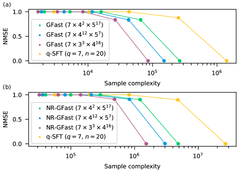
Figure 2: NMSE of GFast compared to $q$-SFT on synthetically generated data, where the Fourier coefficients live in $\mathbb{Z}_{q_{1}=7}\times\mathbb{Z}_{q_{2}=3}\times\mathbb{Z}_{q_{3}=3}\times\mathbb{Z}_{q_{4}=3}\times\mathbb{Z}_{q_{5}=4}\times\cdots\times\mathbb{Z}_{q_{20}=4}$, in the (a) noiseless and (b) noisy settings at various sample complexities. When achieving an NMSE of less than $0.01$, GFast uses up to $16\times$ fewer samples and runs up to $8$ times faster than $q$-SFT.

We first evaluate the performance of GFast on synthetic data by considering the scenario where four different generalized $q$-ary functions taking in an $n=20$ length sequence have $q_{\text{max}}=7$ (the distribution of alphabets is shown in the legend of Fig. 2a). We run $q$-SFT on one function by setting $q_{i}=q_{\text{max}},\forall i\in 1\dots n$. Following Assumptions 1 and 2, we synthetically generate an $S$-sparse Fourier transform $F$, where $\mathcal{S}=\text{supp}(F)$ is chosen uniformly at random in $\mathbb{Z}_{q_{1}=7}\times\mathbb{Z}_{q_{2}=3}\times\mathbb{Z}_{q_{3}=3}\times\mathbb{Z}_{q_{4}=3}\times\mathbb{Z}_{q_{5}=4}\times\cdots\times\mathbb{Z}_{q_{20}=4}$ with values according to $F[\mathbf{k}]=\rho e^{-j\Omega[\mathbf{k}]}\text{ if }\mathbf{k}\in\mathcal{S},\text{ else }0$, where $\Omega[\mathbf{k}]$ are independent and random variables sampled from $[0,2\pi)$. We evaluate performance using normalized mean-squared error (NMSE), which is calculated as: $\text{NMSE}=\frac{||\hat{F}-F||^{2}}{||F||^{2}}=\frac{||\hat{f}-f||^{2}}{||f||^{2}}$, where $\hat{f}$ is the estimated function using the recovered Fourier coefficients. Fig. 2a and 2b compare GFast and NR-GFast with the noiseless and noise-robust versions of $q$-SFT in terms of sample complexity, respectively. We utilize $q$-SFT’s partial-identity subsampling matrix implementation to match the aliasing pattern derived in Equation (7). In the noiseless setting, $\rho=1$, $S=1000$, and $\sigma^{2}$ such that $\text{SNR}=100$dB. To vary the sampling patterns of $\mathbf{q}$ in the noiseless implementation of GFast, we additionally permute $\mathbf{q}$ and each vector of $\mathbf{k}$ five times per experimental instance. For both algorithms, we vary $b$ from 1 to 5 to get different sample counts. In the noisy setting, we set $\rho=1$, $S=1000$, and $\sigma^{2}$ such that $\text{SNR}=10$dB. We vary $b$ from 1 to 5 and $P_{1}$ from 18 to 20 in both algorithms. Each $q$-SFT and GFast experimental instance is run over three random seeds. When GFast achieves an NMSE of less than $0.01$, there is an average difference of $0.96\pm 0.06$ and $0.92\pm 0.06$ in NMSE at the closest sample complexity of $q$-SFT in the noiseless and noisy settings, respectively. When both GFast and $q$-SFT achieve an NMSE of less than $0.01$, GFast uses up to $16\times$ fewer samples and runs up to $8\times$ faster.

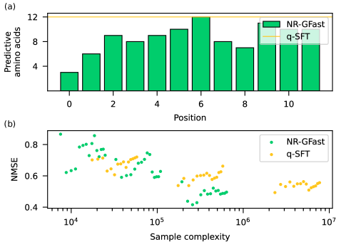
Figure 3: (a) Distribution of predictive amino acids per position that comprise the generalized $q$-ary function in NR-GFast for $n=12$ compared to the $q$-ary function where $q=12$. (b) Performance of $q$-SFT and GFast on florescence in protein sequences as predicted by a trained MLP. Given a sample budget of $10^{6}$, NR-GFast achieves a lower minimal NMSE ($0.42$) than $q$-SFT ($0.54$).

We additionally show the performance of NR-GFast in learning a real-world function. We consider a multilayer perceptron (MLP) trained to predict fluorescence values of green fluorescence protein amino acid sequences [15], where we aim to learn the function $f$ by mutating the first $n=12$ amino acids of the sequence. Using the weights of the first layer, where each amino acid is one-hot encoded as a vector of length 20 (for 20 amino acids), we identify the amino acids at each position most predictive of fluorescence by applying a threshold of 0.05. Fig. 3a shows the distribution of predictive amino acids, where the maximum alphabet size is $q=12$. By treating this problem as a generalized $q$-ary function, we reduce the dimensionality of the problem from $q^{n}=12^{12}\sim 8.9\times 10^{12}$ down to $8.6\times 10^{10}$. We run NR-GFast on the most predictive amino acids in $\mathbb{Z}_{\mathbf{q}}$ and $q$-SFT using $q=12$ and $n=20$, and calculate the test NMSE of both algorithms on a $10,000$ samples chosen uniformly and randomly from $\mathbb{Z}_{\mathbf{q}}$. We vary $b$ from 1 to 3 and $P_{1}$ from $5$ to $20$ in both algorithms to get different sample complexities.

Fig. 3b compares NR-GFast with $q$-SFT. Given a sample budget of $10^{6}$ samples, NR-GFast achieves a minimal NMSE of $0.42$, while $q$-SFT achieves a minimal NMSE of $0.54$. Although $q$-SFT was allowed to run at sample complexities up to $10^{7}$, the minimal NMSE ($0.49$) is still worse than NR-GFast. These results together highlight the sample efficiency of NR-GFast.

6 Conclusion and Future Work

In this paper, we introduced GFast, a fast and efficient algorithm for computing the sparse Fourier transform of generalized $q$-ary functions. Our theoretical analysis and empirical experiments demonstrate that GFast outperforms existing algorithms limited to $q$-ary functions by achieving faster computation and requiring fewer samples, especially when the alphabet size distribution is non-uniform. This advantage arises because non-uniform alphabets effectively reduce the problem’s dimensionality.

Several promising research directions remain to be explored. For example, our theoretical analysis with noise assumes bounded $q_{i}$, and our experiments are limited to alphabet sizes smaller than $20$. A significant increase in $q$, for example, to several thousand in language processing applications, will degrade GFast’s performance. Developing algorithms that are robust to large alphabets is an important future challenge. Additionally, leveraging GFast to develop methods for explaining large-scale machine learning models of generalized $q$-ary functions—such as those used in biology and natural language processing—offers another exciting avenue for further research.

7 Appendix

7.1 Proof of Equation (7)

Proof.

Let us first examine the case with no delay:

$$U_{c,p}[\mathbf{j}]=\frac{1}{B_{c}}\sum_{\bm{\ell}\in\mathbb{Z}_{\mathbf{b}_{c}}}f(\mathbf{M}_{c}\bm{\ell})\prod_{m=1}^{b}\omega_{\left(\mathbf{b}_{c}\right)_{i}}^{-j_{m}\ell_{m}}.$$ (14)

Using Equations (3) and (14), this is equivalent to:

$$U_{c,p}[\mathbf{j}]=\frac{1}{B_{c}}\sum_{\bm{\ell}\in\mathbb{Z}_{\mathbf{b}_{c}}}\left(\sum_{\mathbf{k}\in\mathbb{Z}_{\mathbf{q}}}F[\mathbf{k}]\prod_{i=1}^{n}\omega_{q_{i}}^{k_{i}(\mathbf{M}_{c}\bm{\ell})_{i}}\right)\prod_{m=1}^{b}\omega_{\left(\mathbf{b}_{c}\right)_{i}}^{-j_{m}\ell_{m}}.$$ (15)

Using the structure of $\mathbf{M}_{c}$ from Equation (4), we know that $\mathbf{M}_{c}$ will freeze an $n-b$ bit segment of $\mathbf{M}_{c}\bm{\ell}$ to 0, which lets us rewrite Equation (15) as:

$$U_{c,p}[\mathbf{j}]=\frac{1}{B_{c}}\sum_{\mathbf{k}\in\mathbb{Z}_{\mathbf{q}}}F[\mathbf{k}]\sum_{\bm{\ell}\in\mathbb{Z}_{\mathbf{b}_{c}}}\prod_{m=1}^{b}\omega_{\left(\mathbf{b}_{c}\right)_{i}}^{\ell_{m}((\mathbf{M}_{c}^{T}\mathbf{k})_{m}-j_{m})}=\sum_{\mathbf{k}:\mathbf{M}_{c}^{T}\mathbf{k}=\mathbf{j}}F[\mathbf{k}],$$ (16)

where the last step uses Lemma 3. We can then use the shifting property of the Fourier transform to get the pattern with the delay:

$$U_{c,p}[\mathbf{j}]=\sum_{\mathbf{k}:\text{ }\mathbf{M}_{c}^{T}\mathbf{k}=\mathbf{j}}F[\mathbf{k}]\prod_{i=1}^{n}\omega_{q_{i}}^{(\mathbf{d}_{c,p})_{i}k_{i}}.$$ (17)

∎

Lemma 3.

For some vector $\mathbf{a}\in\mathbb{Z}_{\mathbf{v}}=\mathbb{Z}_{v_{1}}\times\mathbb{Z}_{v_{2}}\times\cdots\mathbb{Z}_{v_{n}}$,

$$\sum_{\bm{\ell}\in\mathbb{Z}_{\mathbf{v}}}\prod_{i=1}^{n}\omega_{v_{i}}^{\ell_{i}a_{i}}=0\Leftrightarrow\mathbf{a}\neq\mathbf{0}.$$ (18)

Proof.

If we let $\mathbf{a}=\mathbf{0}$, then the product term becomes:

$$\prod_{i=1}^{n}\omega_{v_{i}}^{\ell_{i}(0)}.$$

This product reduces to 1, which simplifies Equation (18) to:

$$\sum_{\bm{\ell}\in\mathbb{Z}_{\mathbf{v}}}1=v_{1}v_{2}\cdots v_{n}.$$

For $\mathbf{a}\neq\mathbf{0}$, we can then rewrite Equation (18) as:

$$\prod_{i=1}^{n}\sum_{\ell_{j}\in\mathbb{Z}_{v_{i}}}\omega_{v_{i}}^{\ell_{j}a_{i}}.$$

The summation term is a sum over all of the roots of unity of $\omega_{v_{i}}$, which comes out to 0. This makes the entire expression equal 0. ∎

7.2 Proof of Theorem 1

Our proof follows a similar structure to those seen in other papers that analyze low-density parity check (LDPC) codes. First, we find the general distribution of check nodes in the graph and show that the expected number of Fourier coefficients not recovered converges to 0 given sufficient samples. Then, we use a martingale argument to show that the number of Fourier coefficients not recovered converges to its mean. Lastly, we show that peeling is always possible by showing that any subset of the variable nodes makes an expander graph.

Lemma 4.

Let $c$ be an arbitrary subsampling group where the alphabet subset is defined as seen in Equation (5). Then, the fraction of edges connected to check nodes in $c$ with degree $j$ can be written as:

$$\rho_{c,j}=\frac{(1/\eta_{c})^{j-1}e^{-1/\eta_{c}}}{(j-1)!}\quad j=0,\cdots,S$$ (19)

Proof.

Let $\mathcal{G}(S,\{\eta_{c}\}_{c\in[C]},C,\{{\mathbf{M}}_{c}\}_{c\in[C]})$ represent the set of all bipartite graphs from subsampling matrices $\mathbf{M}_{c}$. We again assume that the subsampling matrices are constructed according to Equation (4). This lets us assume that for a certain $c$ where $\mathbf{j}=\mathbf{M}_{c}\mathbf{k}$, each $\mathbf{j}_{c}$ is chosen uniformly and randomly from $\mathbb{Z}_{\mathbf{b}_{c}}$. For each group $c\in[C]$, let $\eta_{c}$ be a redundancy parameter such that $B_{c}=S\eta_{c}$. The proof for this closely follows Appendix B.1 of [25], except we analyze the degree distribution of the bipartite graph for each group $c$, rather than the entire graph, because the bipartite graph is biased by the varied alphabet size and size of $B_{c}$ for each group. For a single group $c$, with total number of hashed coefficients $B_{c}$, we have $S$ edges. This means that for a certain group $c$, the fraction of edges connecting to check nodes with degree $j$ is:

$$\rho_{c,j}=\frac{\text{Pr(check node has degree }j)B_{c}j}{S}=\text{Pr(check node has degree }j)\eta_{c}j.$$

Since the probability of some arbitrary edge $e$ being connected to a check node $\mathbf{j}$ is $1/B_{c}$, which means that the probability that $\mathbf{j}$ has degree $j$ can be found with a binomial distribution: $Binom(\frac{1}{\eta_{c}}S,S)$, we can approximate this by a Poisson distribution:

$$\text{Pr(check node has degree }j)=\frac{(1/\eta_{c})^{j}e^{-1/\eta_{c}}}{j!}.$$

This gives us the result seen in Equation (19).
∎

Figure 4: Directed neighborhood $\mathcal{N}_{e}^{2i}$ of depth 2 for an edge $e$ over a particular graph $\mathcal{G}(S,\{\eta_{c}\}_{c\in[C]},C,\{{\mathbf{M}}_{c}\}_{c\in[C]})$ with $C=4$ subsampling groups. Dotted lines represent edges peeled on the last iteration. $c$ could be peeled from the graph on the next iteration because check node $c^{\prime}$ now has degree 1.

For the next step, we will analyze the density evolution of the peeling decoder [28]. Let $\mathcal{N}_{e}^{\ell}$ be the directed neighborhood of edge $e$ with depth $\ell$, which can be written as $e_{1},e_{2},\cdots e_{\ell},e\neq e_{1}$, an example of which can be seen in Fig. 4. Given the local cycle-free neighborhood $\mathcal{N}_{e}^{2i}$ of an edge $e=(v,c^{\prime})$, we can find the probability $p_{c,i}$ that $e$ is present after $i$ iterations as:

$$p_{c^{\prime},i}=\prod_{c\in[C]\setminus\{c^{\prime}\}}(1-\sum_{j}\rho_{c,j}(1-p_{c,i-1})^{j-1}),$$ (20)

where $[C]=\{1,\ldots,C\}$. This can further be approximated as:

$$p_{c^{\prime},i}=\prod_{c\in[C]\setminus\{c^{\prime}\}}(1-e^{\frac{1}{\eta_{c}}p_{c,i-1}}),$$ (21)

due to the Poisson distribution of the check nodes [23]. It is possible to choose $\{\eta_{c}\}_{c\in[C]}$ such that $p_{c,i}$ converges to 0 for all $c$. Table 1 of [25] gives the values of $\eta$ needed for convergence for a certain value of $C$. In our case, it is possible to find similar values of $\eta_{c}$ that cause convergence.

Then, let $\mathcal{T}_{i}$ be the event that for every edge $e$ the neighborhood $\mathcal{N}_{e}^{2i}$ is a tree, and let $Z_{i}$ be the number of edges that are still not peeled after iteration $i$, such that $Z_{i}=\sum_{c^{\prime}\in[C]}\sum_{e}Z_{i}^{e_{c^{\prime}}}$, where $Z_{i}^{e_{c^{\prime}}}=\mathbbm{1}\{\text{Edge }e\text{ in group }c^{\prime}\text{ is not peeled}\}$. Then, the expected number of edges not peeled can be written as:

$$\mathbbm{E}[Z_{i}|\mathcal{T}_{i}]=S\sum_{c=1}^{C}p_{c,i}.$$ (22)

This shows that, given that the neighborhoods are all trees, we can terminate the peeling operation for an arbitrarily small number of edges left: $Z_{i}<\epsilon S\sum_{c=1}^{C}p_{c,i}$. We show in Lemma 8 that the probability all neighborhoods $\mathcal{N}_{e}^{2i}$ are trees increases as $S$ increases. We can show that the difference between the expectation and the expectation conditioned on the tree assumption can be made arbitrarily small:

Lemma 5.

(Adapted from Lemma 10 of [29]) For some peeling iteration $i>0$, $\exists\epsilon>0,S:|\mathbb{E}[Z_{i}]-\mathbb{E}[Z_{i}|\mathcal{T}_{i}]|\leq SC\epsilon/2$

Proof.

Due to linearity of expectation, we can write that $\mathbb{E}[Z_{i}]=S\sum_{c^{\prime}\in[C]}\mathbb{E}[Z_{i}^{e_{c^{\prime}}}].$ This proof stays the same regardless of the check node group that edge $e$ is connected to, so we will drop the $c^{\prime}$ subscript. We can then use total expectation to rewrite $\mathbb{E}[Z_{i}^{e}]$:

$$\mathbb{E}[Z_{i}^{e}]=\mathbb{E}[Z_{i}^{e}|\mathcal{T}_{i}]\text{Pr}(\mathcal{T}_{i})+\mathbb{E}[Z_{i}^{e}|\mathcal{T}_{i}^{c}]\text{Pr}(\mathcal{T}_{i}^{c}).$$ (23)

Trivially, we know that $\mathbb{E}[Z_{i}^{e}|\mathcal{T}_{i}^{c}]\leq 1$. We also know that $\mathbb{E}[Z_{i}^{e}|\mathcal{T}_{i}]=p_{c,i}$. Using the definition of $\mathbb{E}[Z_{i}|\mathcal{T}_{i}]$ given in Equation (22), we can bound $\mathbb{E}[Z_{i}]$ as,

$$\mathbb{E}[Z_{i}|\mathcal{T}_{i}]-SC\text{Pr}(\mathcal{T}_{i}^{c})\leq\mathbb{E}[Z_{i}]\leq\mathbb{E}[Z_{i}|\mathcal{T}_{i}]+SC\text{Pr}(\mathcal{T}_{i}^{c}).$$ (24)

From Lemma 8, we know that $\text{Pr}(\mathcal{T}_{i})=1-O(\log^{i}(S)/S)$, which we can rewrite as $1-\gamma\frac{\log^{i}(S)}{S}$ for some constant $\gamma$. With a little algebra, we can get:

$$-C\gamma\log^{i}(S)\leq\mathbb{E}[Z_{i}]-\mathbb{E}[Z_{i}|\mathcal{T}_{i}]\leq C\gamma\log^{i}(S),$$

which simplifies to $|\mathbb{E}[Z_{i}]-\mathbb{E}[Z_{i}|\mathcal{T}_{i}]|\leq SC\epsilon/2$ given that $\frac{S}{\log^{i}(S)}\geq 2\gamma/\epsilon$. ∎

Now that we have shown that we can make the mean arbitrarily small, we would like to show that the number of unpeeled edges will converge to its mean value. To show convergence around the mean, we will set up a martingale $Y_{1},\cdots Y_{SC}$, where $Y_{\ell}=\mathbb{E}[Z_{i}|Z_{1}^{i},Z_{2}^{i},\cdots Z_{\ell}^{i}]$ such that $Y_{0}=\mathbb{E}[Z_{i}]$ and $Y_{SC}=\mathbb{E}[Z_{i}|Z_{1}^{i},Z_{2}^{i}\cdots Z_{SC}^{i}]=Z_{i}$. This is a Doob’s martingale process, which means we can apply Azuma’s inequality:

$$\text{Pr}(|Z_{i}-\mathbb{E}[Z_{i}]|>t)\leq 2\exp\left(-\frac{t^{2}}{2\sum_{i=1}^{SC}\alpha_{i}^{2}}\right).$$ (25)

We must first find the finite difference $|Y_{i}-Y_{i-1}|=\alpha_{i}$. It was shown in Theorem 2 of [30] that, for a Tanner graph with regular variable degree $d_{V}$ and regular check degree $d_{C}$, $\alpha_{i}$ would be upper bounded by $8(d_{V}d_{C})^{i}$. However, as seen in Equation (19), the check node degree distribution of $\mathcal{G}(S,\{\eta_{c}\}_{c\in[C]},C,\{{\mathbf{M}}_{c}\}_{c\in[C]})$ is not uniform, so we must adjust for the irregular degrees of the check node.

Lemma 6.

Using the definition of Azuma’s inequality given in Equation (25), we can bound the finite martingale difference as $\alpha_{i}^{2}=O(S^{\frac{4i}{4i+1}})$.

Proof.

We will first find the probability of $d_{C}\geq O(S^{\frac{2}{4i+1}})$. Then, for some constants $d_{1},d_{2},\beta$, we can bound this probability first using a Chernoff bound for a Poisson random variable $X$ with mean $\lambda$:

$$\text{Pr}(X>d_{1}S^{\frac{2}{4i+1}})\leq\left(\frac{e\lambda}{d_{1}S^{\frac{2}{4i+1}}}\right)^{d_{1}S^{\frac{2}{4i+1}}}.$$ (26)

Then, we can bound the right-hand side as:

$$\left(\frac{e\lambda}{d_{1}S^{\frac{2}{4i+1}}}\right)^{d_{1}S^{\frac{2}{4i+1}}}\leq d_{2}\exp(-\beta S^{\frac{2}{4i+1}}).$$ (27)

Note that this applies for all groups $c$ since every group has Poisson distributed check node degrees. Now, let $\mathcal{B}$ be the event that at least one check node has a degree more than $O(S^{\frac{2}{4i+1}})$. Given the result of Equation (27) and using a union bound across all the nodes in $B_{c}=\eta_{c}S$, we can write:

$$\text{Pr}(\mathcal{B})<d_{3}S\exp(-\beta S^{\frac{2}{4i+1}}).$$

Let $\mathcal{B}^{c}$ be the event that no check node has a degree more than $O(S^{\frac{1}{4i+1}})$. If $\mathcal{B}$ has not happened, then we can bound $d_{C}$ by,

$$d_{C}\leq O(S^{\frac{2}{4i+1}}),$$

and get a finite difference,

$$\alpha_{i}^{2}=(8(d_{V}d_{C})^{i})^{2}=O(S^{\frac{4i}{4i+1}}).$$

∎

With this result we can look closer at the concentration around the mean:

Lemma 7.

(Adapted from [25]) For some constant $\beta$, $\text{Pr}(|Z_{i}-\mathbb{E}[Z_{i}]|>CS\epsilon/2)\leq 2\exp(-\beta\epsilon^{2}S^{\frac{1}{4i+1}}).$

Proof.

Using the law of total probability, we can rewrite the probability as:

$$\text{Pr}(|Z_{i}-\mathbb{E}[Z_{i}]|>CS\epsilon/2)=\text{Pr}(|Z_{i}-\mathbb{E}[Z_{i}]|>CS\epsilon/2\ |\ \mathcal{B})\text{Pr}(\mathcal{B})+\text{Pr}(|Z_{i}-\mathbb{E}[Z_{i}]|>CS\epsilon/2\ |\ \mathcal{B}^{c})\text{Pr}(\mathcal{B}^{c}),$$

which can once again be bounded with,

$$\text{Pr}(|Z_{i}-\mathbb{E}[Z_{i}]|>CS\epsilon/2)\leq\text{Pr}(\mathcal{B})+\text{Pr}(|Z_{i}-\mathbb{E}[Z_{i}]|>CS\epsilon/2\ |\ \mathcal{B}^{c}).$$ (28)

Now, we can use the result from Lemma 6 to bound the right-hand side of Equation (28) as:

$$\text{Pr}(|Z_{i}-\mathbb{E}[Z_{i}]|>CS\epsilon/2\ |\ \mathcal{B}^{c})+\text{Pr}(\mathcal{B})\leq 2\exp\left(\frac{-C^{2}S^{2}\epsilon^{2}}{8\sum_{i=1}^{SC}\alpha_{i}^{2}}\right)+d_{3}S\exp(-\beta S^{\frac{2}{4i+1}}).$$ (29)

Since the slowest growing exponential in Equation (29) is $S^{\frac{2}{4i+1}}$, we can again lower bound the right-hand side to get the result:

$$\text{Pr}(|Z_{i}-\mathbb{E}[Z_{i}]|>CS\epsilon/2)\leq 2\exp(-\beta\epsilon^{2}S^{\frac{1}{4i+1}}).$$

∎

Lemma 8.

(Adapted from [29]) For a sufficiently large $S$, all neighborhoods $\mathcal{N}_{e}^{2i}$ are trees.

Proof.

To prove that $\mathcal{N}_{e}^{2i}$ is a tree for all $i$, we start with a fixed $\mathcal{N}_{e}^{2i}$ that is a tree approaching $i^{*}>i$. Let $C_{i}$ be the number of check nodes in group $c$ and $V_{i}$ be the number of variable nodes in the tree at this point. We will start by showing that, with a high probability, the size of the tree neighborhood grows slower than $O(\log^{i}(S))$. Using the law of total probability, we can write:

$$\text{Pr}(\mathcal{T}_{i}^{c})\leq\text{Pr}(V_{i}>\kappa_{1}\log^{i}(S))+\text{Pr}(C_{i}>\kappa_{2}\log^{i}(S))+\text{Pr}(\mathcal{T}_{i}^{c}\ |\ Vi<\kappa_{1}\log^{i}(S),C_{i}>\kappa_{2}\log^{i}(S))).$$ (30)

If we denote $\alpha_{i}=\text{Pr}(V_{i}>\kappa_{1}\log^{i}(S))$, then we bound $\alpha_{i}$ as:

$$\alpha_{i} \leq\alpha_{i-1}+\text{Pr}(V_{i}>\kappa_{1}\log^{i}(S)\mid V_{i-1}<\kappa_{1}\log^{i}(S))$$

$$\leq\alpha_{i-1}+\text{Pr}(V_{i}>\kappa_{1}\log^{i}(S)\mid C_{i-1}<\kappa_{2}\log^{i}(S)),$$ (31)

where the last inequality comes from the fact that for each variable node added to the tree, $C-1$ check nodes are also added to the tree. To bound the last term in Equation (31), we would need to analyze the degree distribution of each check node. We will examine the number of check nodes at exactly depth $i$ in the graph $M_{i}$, where $M_{i}<C_{i}$. Let $D_{i}$ be the degree of each check node. Finding the probability that $V_{i}>\kappa_{1}\log^{i}(S)$ is equivalent to finding the probability that $\sum_{j}D_{j}>\kappa_{3}\log^{i}(S)$ since each edge of each $M_{i}$ check nodes is connected to a variable node in $V_{i}$. Therefore, we can bound the right-hand side of Equation (31) as:

$$\text{Pr}(V_{i}>\kappa_{1}\log^{i}(S)\ |\ C_{i-1}<\kappa_{2}\log^{i}(S))\leq\text{Pr}\left(\sum_{j=i}^{M_{i}}D_{j}\geq\kappa_{3}\log^{i}(S)\right).$$ (32)

We know that check node degrees are Poisson distributed, but each group $c$ has a different mean $1/\eta_{c}$. For an accurate bound, we will assume all check node degrees are Poisson distributed with the highest mean from $\{\frac{1}{\eta_{c}}\}_{c\in[C]}$. Let $D_{j,c_{max}}$ denote the degree of a check node from group $c_{\text{max}}\coloneqq\operatorname*{arg\,max}_{c}(1/\eta_{c})$. Then, we can write a final bound as:

$$\text{Pr}\left(\sum_{j=i}^{M_{i}}D_{j}\geq\kappa_{3}\log^{i}(S)\right)\leq\text{Pr}\left(\sum_{j=i}^{M_{i}}D_{j,c_{\text{max}}}\geq\kappa_{3}\log^{i}(S)\right)\leq\left(\frac{eM_{i}/\eta_{c_{\text{max}}}}{\kappa_{3}\log^{i}(S)}\right)^{\kappa_{3}\log^{i}(S)}\leq O(1/S),$$ (33)

meaning that $\alpha_{i}\leq\alpha_{i-1}+O(1/S)$. Since we can bound the number of variable nodes in the graph with this high probability, we know that the same bound applies to the check nodes. Now that we have shown that the tree grows no larger than $O(\log^{i}(S))$ with probability $1/S$, we can move on to the probability of creating a tree. The rest of the proof follows closely from [30], other than the assumption of uniform check node degree.

Let $C_{i,c}$ be the number of check nodes from group $c$ present in the graph. Let $t$ be the number of new edges to check nodes in $c$ from the variable nodes in $\mathcal{N}_{e}^{2i+1}$ that do not create a loop. Then, the probability that the next revealed edge does not create a loop is:

$$\frac{B_{c}-C_{i,c}-t}{B_{c}}\geq 1-\frac{C_{i^{*},c}}{B_{c}},$$

where $c$ is the group that the next edge connects to, and assuming that $i^{*}$ is sufficiently large. If $\mathcal{N}_{e}^{2i}$ is a tree, then the probability that $\mathcal{N}_{e}^{2i+1}$ is a tree depends on whether all the new edges from the variable nodes in $\mathcal{N}_{e}^{2i}$ connect to check nodes that were not already in the tree. We can lower bound the probability as the following:

$$\text{Pr}(\mathcal{N}_{e}^{2i+1}\text{ is tree-like }|\ \mathcal{N}_{e}^{2i}\text{ is tree-like })\geq\min_{c}\left(1-\frac{C_{i^{*},c}}{B_{c}}\right)^{C_{i+1,c}-C_{i,c}}.$$

If we then assume that $\mathcal{N}_{e}^{2i+1}$ is a tree, the probability of whether $\mathcal{N}_{e}^{2i+2}$ is a tree can be found similarly. Assuming that $k$ edges have been revealed going from check nodes to variable nodes at depth $2i+2$ without creating a loop, the probability of the next edge creating a loop is:

$$\frac{(S-V_{i}-k)C}{SC-V_{i}-k}\geq\left(1-\frac{V_{i}^{*}}{S}\right).$$

This similarly gives a lower bound on the probability:

$$\text{Pr}(\mathcal{N}_{e}^{2i+2}\text{ is tree-like }|\ \mathcal{N}_{e}^{2i+2}\text{ is tree-like })\geq\left(1-\frac{V_{i^{*}}}{S}\right)^{V_{i+1}-V_{i}}.$$

This means that the probability that $\mathcal{N}_{e}^{2i^{*}}$ is a tree is lower bounded by:

$$\min_{c}\left(1-\frac{C_{i^{*},c}}{B_{c}}\right)^{C_{i^{*},c}}\left(1-\frac{V_{i^{*}}}{S}\right)^{V_{i^{*}}}.$$

For sufficiently large $k$ and fixed $i^{*}$, we can upper bound the probability that $\mathcal{N}_{e}^{2i^{*}}$ is a not tree as:

$$\text{Pr}(\mathcal{N}_{e}^{2i^{*}}\text{ is tree-like})\leq\max_{c}\frac{M_{i^{*}}^{2}+\frac{1}{\eta_{c}}C_{i^{*},c}^{2}}{S}.$$ (34)

We previously showed that check node size at depth $i$ is upper bounded by $O(\log^{i}(S))$ with a high probability, which means that we can bound Equation (34) again as:

$$\text{Pr}(\mathcal{N}_{e}^{2i^{*}}\text{ is tree-like})\leq O(\log^{i^{*}}(S)/S).$$ (35)

∎

Definition 7.1.

(Adapted from [25]) Consider a subset $\mathcal{S}$ of $\mathcal{G}(S,\{\eta_{c}\}_{c\in[C]},C,\{{\mathbf{M}}_{c}\}_{c\in[C]})$ with $|\mathcal{S}|=k<\epsilon S$. If, for a neighborhood of check nodes in group $c$ $\mathcal{N}_{c}(\mathcal{S})$, the condition is met that $|\mathcal{N}_{c}(\mathcal{S})|>|\mathcal{S}|/2$, then $\mathcal{G}(S,\{\eta_{c}\}_{c\in[C]},C,\{{\mathbf{M}}_{c}\}_{c\in[C]})$ is an $(\epsilon,1/2,C)$-expander.

Lemma 9.

The probability that $\mathcal{G}(S,\{\eta_{c}\}_{c\in[C]},C,\{{\mathbf{M}}_{c}\}_{c\in[C]})$ is an expander graph is at least $1-O(1/S)$.

Proof.

Given a subset of the variable nodes $\mathcal{S}$ where $|\mathcal{S}|=k<\epsilon S$, we can make a neighborhood of check nodes $\mathcal{N}_{c}(\mathcal{S})$. The graph $\mathcal{G}(S,\{\eta_{c}\}_{c\in[C]},C,\{{\mathbf{M}}_{c}\}_{c\in[C]})$ is considered an expander graph if $|\mathcal{N}_{c}(\mathcal{S})|\geq k/2$ for at least 1 group $c$. We can write the probability of this as:

$$\text{Pr}(\mathcal{S}\text{ is not an expander})\leq{S\choose k}\prod_{c=1}^{C}{B_{c}\choose k/2}\left(\frac{k}{2Bc}\right)^{k},$$ (36)

where ${S\choose k}$ represents the total number of possible subsets that can be made, ${B_{c}\choose k/2}$ represents the number of possible check node subsets that can be chosen from $B_{c}$, and $\left(\frac{k}{2Bc}\right)^{k}$ represents the probability that the subset of check nodes contains all the neighbors of the vertices in $\mathcal{S}$. Then we can use the inequality that ${a\choose b}\leq(ae/b)^{b}$ to rewrite Equation (36) as:

$$\text{Pr}(\mathcal{S}\text{ is not an expander})\leq\left(\frac{Se}{k}\right)^{k}\left(\frac{ke}{2S}\right)^{Ck/2}\prod_{c=1}^{C}\left(\frac{1}{\eta_{c}}\right).$$

This can again be bounded as:

$$\text{Pr}(\mathcal{S}\text{ is not an expander})\leq\left(\frac{k}{S}\right)^{k(\frac{C}{2}-1)}c^{k},\quad c=e\left(\prod_{c=1}^{C}\left(\frac{e}{\eta_{c}}\right)\right)^{1/2}.$$ (37)

Given that $\frac{C}{2}-1\geq\frac{1}{2}$, we can bound the probability again as:

$$\text{Pr}(\mathcal{S}\text{ is not an expander})\leq\left(\frac{kc^{2}}{S}\right)^{k/2}.$$ (38)

Clearly, $\mathcal{S}$ being an expander is dependent on the number of vertices $k$. We can take 2 edge cases where $k=O(S)$ and $k=O(1)$:

$$\text{Pr}(\mathcal{S}\text{ is not an expander})=\begin{cases}e^{-S\log(\frac{1}{\epsilon c^{2}})},\quad k=\epsilon S\text{ with }\epsilon<\frac{1}{2c^{2}}\\ O(1/S),\quad k=O(1).\end{cases}$$ (39)

For the very sparse regime $0\leq\delta\leq 1/3$, we are unlikely to see case 1. Therefore, we can show that $\mathcal{S}$ is an $\epsilon$-expander graph with probability $1-O(1/S)$ in the very sparse regime. For $1/3\leq\delta\leq 1$, it is possible to see both cases. In this case, the probability could either be $1-O(1/S)$ or $1-e^{-S\log(\frac{1}{\epsilon c^{2}})}$, but since $1-e^{-S\log(\frac{1}{\epsilon c^{2}})}$ converges to 0 more quickly, we use $O(1/S)$ in Theorem 1. ∎

If we have an expander graph, that means that the average degree within at least one group $c$ is less than 2, meaning at least 1 group $c$ has a singleton that can be peeled. This allows for another iteration of peeling. The number of samples required for the algorithm scales with $O(P\sum_{c=1}^{C}B_{c})=O(Sn)$. The computational complexity is $O(PB\log B)=O(Sn\log S)=O(Sn\log N)$ since $S=O(N^{\delta})$.

7.3 Proof of Proposition 1

Proof.

Given a singleton pair $(\mathbf{k},F[\mathbf{k}])$ in group $c$, the angle quantization is written as:

$$\text{arg}[U_{p}]=\text{arg}[F[\mathbf{k}]]+\left(\sum_{i=1}^{n}\frac{2\pi}{q_{i}}(\mathbf{d}_{p})_{i}k_{i}\right)+Y_{p},$$ (40)

where $Y_{p}$ is a uniform random variable over $[-\pi,\pi)$. Similarly, for $U_{p,r}$, we have:

$$\text{arg}[U_{p,r}]=\text{arg}[F[\mathbf{k}]]+\left(\sum_{i=1}^{n}\frac{2\pi}{q_{i}}(\mathbf{d}_{p,r})_{i}k_{i}\right)+Y_{p,r},$$ (41)

where $\frac{2\pi}{q_{i}}(\mathbf{d}_{p,r})_{i}k_{i}=\frac{2\pi}{q_{i}}(\mathbf{d}_{p})_{i}k_{i}$ for all $i\neq r$ and $Y_{p,r}$ is another uniform random variable over $[-\pi,\pi)$. The ratio of the 2 quantized angles is written as,

$$\text{arg}[U_{p,r}/U_{p}]=\frac{2\pi}{q_{r}}k_{r}+Y_{p,r}-Y_{p},$$ (42)

which satisfies:

$$\text{Pr}(|Y_{p}|\geq\alpha)\leq\text{Pr}(|W_{p}|\geq|F[\mathbf{k}]|\sin(\alpha))$$

for $0\leq\alpha\leq\pi/2$. Using the definition of a Rayleigh random variable, the right-hand side is bounded by:

$$\text{Pr}(|W_{p}|\geq F[\mathbf{k}]\sin(\alpha))\leq\exp\left(-\frac{|F[\mathbf{k}]|^{2}\sin^{2}(\alpha)}{2\sigma^{2}/B}\right)=\exp\left(-\frac{\eta\sin^{2}(\alpha)\text{SNR}}{2}\right).$$ (43)

The final result is obtained as:

$$\begin{split}\text{Pr}(|Y_{p,r}-Y_{p}|\geq\pi/2q_{r})\leq\text{Pr}(|Y_{p,r}|\geq\pi/2q_{r})+\text{Pr}(|Y_{p}|\geq\pi/2q_{r})\leq\\ 2\exp\left(-\frac{\eta\sin^{2}(\pi/2q_{r})\text{SNR}}{2}\right).\end{split}$$ (44)

∎

7.4 Proof of Theorem 2

Throughout this proof, we assume that each $q_{i}$ is a fixed constant (i.e., $q_{i}=O(1)\ \forall i\in 1\dots n$). This lets us assume that $\log N=O(n)$, which will be necessary throughout this proof. We also drop the $c$ notation as all analysis is within a certain group, and is the same regardless of group.

Proposition 2.

Let $\mathbb{P}_{F}$ be the probability that the robust bin detection algorithm makes an error in $CS=O(S)$ iterations (i.e. $F\neq\hat{F}$) within some group $c$. The probability of error can be bounded as:

$$\mathbb{P}_{F}\leq O(1/S).$$

Proof.

Using the law of total probability, we rewrite the probability that NR-GFast fails as:

$$\text{Pr}(\hat{F}\neq F)=\text{Pr}(\hat{F}\neq F\ |\ \mathcal{E})\text{Pr}(\mathcal{E})+\text{Pr}(\hat{F}\neq F\ |\ \mathcal{E}^{c})\text{Pr}(\mathcal{E}^{c}),$$ (45)

which can again be bounded as

$$\text{Pr}(\hat{F}\neq F)\leq\text{Pr}(\mathcal{E})+\text{Pr}(\hat{F}\neq F\ |\ \mathcal{E}^{c}).$$ (46)

We can use the result of Theorem 1 showing that $\text{Pr}(\hat{F}\neq F\ |\ \mathcal{E}^{c})=O(1/S)$. Next, we must show that $\text{Pr}(\mathcal{E})\leq O(1/S)$. Let $\mathcal{E}_{b}$ be the event of an error happening for a specific bin. Then, we can union bound over all bins in $c$ and all iterations to get a bound on $\text{Pr}(\mathcal{E})$:

$$\text{Pr}(\mathcal{E})\leq CS^{2}\eta_{c}\text{Pr}(\mathcal{E}_{b}).$$ (47)

Therefore, to show that $\text{Pr}(\mathcal{E})\leq O(1/S)$, we must show that $\text{Pr}(\mathcal{E}_{b})\leq O(1/S^{3})$. Using the law of total probability, we rewrite $\text{Pr}(\mathcal{E}_{b})$ as:

$$\text{Pr}(\mathcal{E}_{b})\leq\sum_{\mathcal{F}\in\{\mathcal{H}_{m},\mathcal{H}_{Z}\}}\text{Pr}(\mathcal{F}\leftarrow\mathcal{H}_{S}(\mathbf{k},F[\mathbf{k}]))+\sum_{\mathcal{F}\in\{\mathcal{H}_{m},\mathcal{H}_{Z}\}}\text{Pr}(\mathcal{H}_{S}(\mathbf{k},F[\mathbf{k}])\leftarrow\mathcal{F})+\text{Pr}((\hat{\mathbf{k}},\hat{F}[\hat{\mathbf{k}}])\leftarrow(\mathbf{k},F[\mathbf{k}])).$$ (48)

Here, the following events are represented:

1. The event $\mathcal{F}\leftarrow\mathcal{H}_{S}(\mathbf{k},F[\mathbf{k}])$ represents a singleton bin being incorrectly classified as a zero-ton or multi-ton.

2. The event $\mathcal{H}_{S}(\mathbf{k},F[\mathbf{k}])\leftarrow\mathcal{F}$ represents a zero-ton or multi-ton being incorrectly classified as a singleton.

3. The event $(\hat{\mathbf{k}},\hat{F}[\hat{\mathbf{k}}])\leftarrow(\mathbf{k},F[\mathbf{k}])$ represents a singleton bin being classified with an incorrect index and value pair.

It is shown in Propositions 3, 4, and 5 that the probabilities of each of these events decrease exponentially with respect to $P_{1}$, so setting $P_{1}=O(n)=O(\log N)$ lets us bound $\text{Pr}(\mathcal{E}_{b})\leq O(1/N^{3})$, and since $S$ is sublinear in $N$, this can be used to get the original result $\text{Pr}(\mathcal{E})\leq S^{2}\sum_{c=1}^{C}\eta_{c}\text{Pr}(\mathcal{E}_{b})\leq O(1/S)$. We note that the sample complexity is $O(P\sum_{c=1}^{C}B)=O(P_{1}nS)=O(Sn^{2})$, and the computational complexity is $O(PB\log B)=O(P_{1}nS\log S)=O(Sn^{2}\log N)$. ∎

Proposition 3.

The probability of the event $\mathcal{H}_{S}(\mathbf{k},F[\mathbf{k}])\leftarrow\mathcal{H}_{Z}$ is upper bounded by $\exp\left(-\frac{P_{1}}{2}(\sqrt{1+2\gamma}-1)^{2}\right)$, and the probability of the event $\mathcal{H}_{S}(\mathbf{k},F[\mathbf{k}])\leftarrow\mathcal{H}_{M}$ is upper bounded by $S^{2}\exp\left(-\epsilon\left(1-\frac{2\gamma\nu^{2}}{L\rho^{2}}\right)^{2}P_{1}\right)$.

Proof.

Let us start with the event that a zero-ton is incorrectly identified as a singleton:

$$\text{Pr}(\mathcal{H}_{S}(\hat{\mathbf{k}},\hat{F}[\hat{\mathbf{k}}])\leftarrow\mathcal{H}_{Z})\leq\text{Pr}\left(\frac{1}{P}||\mathbf{W}||^{2}\geq(1+\gamma)\nu^{2}\right).$$ (49)

By applying Lemma 11, we bound the probability of this event as:

$$\text{Pr}(\mathcal{H}_{S}(\hat{\mathbf{k}},\hat{F}[\hat{\mathbf{k}}])\leftarrow\mathcal{H}_{Z})\leq\text{Pr}\left(\frac{1}{P_{1}}||\mathbf{W}||^{2}\geq(1+\gamma)\nu^{2}\right)\leq\exp\left(-\frac{P_{1}}{2}(\sqrt{1+2\gamma}-1)^{2}\right),$$ (50)

where we let $\mathbf{g}=\mathbf{0}$ and $\mathbf{v}=\mathbf{W}$. Next, we will examine the event that a multi-ton is incorrectly identified as a singleton.

$$\text{Pr}(\mathcal{H}_{S}(\hat{\mathbf{k}},\hat{F}[\hat{\mathbf{k}}])\leftarrow\mathcal{H}_{M})\leq\text{Pr}\left(\frac{1}{P_{1}}||\mathbf{g}+\mathbf{W}||^{2}\leq(1+\gamma)\nu^{2}\right),$$ (51)

where $\mathbf{g}=\mathbf{S}(\bm{\alpha}-\hat{F}[\hat{\mathbf{k}}]\mathbf{e}_{\hat{\mathbf{k}}})$. This can again be upper bounded using the law of total probability:

$$\text{Pr}(\mathcal{H}_{S}(\hat{\mathbf{k}},\hat{F}[\hat{\mathbf{k}}])\leftarrow\mathcal{H}_{M})\leq\text{Pr}\left(\frac{1}{P_{1}}||\mathbf{g}+\mathbf{W}||^{2}\leq(1+\gamma)\nu^{2}\,\big{|}\,\frac{\|\mathbf{g}\|^{2}}{P_{1}}\geq 2\gamma\nu^{2}\right)+\text{Pr}\left(\frac{\|\mathbf{g}\|^{2}}{P_{1}}\leq 2\gamma\nu^{2}\right).$$ (52)

From Lemma 11, we know that the left term can be bounded as $\exp(-\frac{P_{1}\gamma^{2}}{2+8\gamma})$. For the second term, let $\bm{\beta}=\bm{\alpha}-\hat{F}[\hat{\mathbf{k}]}\mathbf{e}_{\hat{\mathbf{k}}}$, and label $\mathbf{g}=\mathbf{S}\bm{\beta}$. Defining $\mathcal{L}\coloneqq\text{supp}(\bm{\beta})$, let $\mathbf{S}_{\mathcal{L}}$ refer to the corresponding columns of $\mathbf{S}$ and $\bm{\beta}_{\mathcal{L}}$ refer to the corresponding elements of $\bm{\beta}$ such that $\mathbf{S}\bm{\beta}=\mathbf{S}_{\mathcal{L}}\bm{\beta}_{\mathcal{L}}$. We consider two scenarios:

• Case 1: $L=|\mathcal{L}|=O(1)$, i.e., the number of multi-tons is some arbitrary constant. We can bound the magnitude of $\|\mathbf{S}\bm{\beta}\|^{2}$ as:

  $$\lambda_{min}(\mathbf{S}_{\mathcal{L}}^{H}\mathbf{S}_{\mathcal{L}})\|\bm{\beta}_{\mathcal{L}}\|^{2}\leq\|\mathbf{S}_{\mathcal{L}}\bm{\beta}_{\mathcal{L}}\|^{2}\leq\lambda_{max}(\mathbf{S}_{\mathcal{L}}^{H}\mathbf{S}_{\mathcal{L}})\|\bm{\beta}_{\mathcal{L}}\|^{2},$$

  which lets us bound $\text{Pr}\left(\frac{\|\mathbf{g}\|^{2}}{P_{1}}\leq 2\gamma\nu^{2}\right)\leq\text{Pr}(\lambda_{min}(\frac{1}{P_{1}}\mathbf{S}_{\mathcal{L}}^{H}\mathbf{S}_{\mathcal{L}})\leq 2\gamma\nu^{2}/(L\rho^{2}))$. The matrix $\frac{1}{P_{1}}\mathbf{S}_{\mathcal{L}}^{H}\mathbf{S}_{\mathcal{L}}\in\mathbb{C}^{L\times L}$ is a Hermitian matrix, which lets us bound $\lambda_{min}(\frac{1}{P_{1}}\mathbf{S}_{\mathcal{L}}^{H}\mathbf{S}_{\mathcal{L}})$ using the Gershgorin circle theorem:

  $$\lambda_{min}(\frac{1}{P_{1}}\mathbf{S}_{\mathcal{L}}^{H}\mathbf{S}_{\mathcal{L}})\geq 1-L\mu,$$

  where $\mu$ is defined as seen in Lemma 10. We can then further bound the probability:

  $$\text{Pr}\left(\frac{\|\mathbf{g}\|^{2}}{P_{1}}\leq 2\gamma\nu^{2}\right)\leq\text{Pr}(1-L\mu\leq 2\gamma\nu^{2}/(L\rho^{2}))=\text{Pr}\left(\mu\geq\frac{1}{L}\left(1-\frac{2\gamma\nu^{2}}{L\rho^{2}}\right)\right).$$ (53)

  Using the results of Lemma 10 and setting $\mu_{0}=\frac{2\gamma\nu^{2}}{L\rho^{2}}$, we get the final bound:

  $$\text{Pr}\left(\frac{\|\mathbf{g}\|^{2}}{P_{1}}\leq 2\gamma\nu^{2}\right)\leq 4L^{2}\exp\left(-\frac{P_{1}}{8L^{2}}\left(1-\frac{2\gamma\nu^{2}}{L\rho^{2}}\right)^{2}\right),$$ (54)

  where $\gamma<\frac{L\rho^{2}}{2\nu^{2}}$.

• Case 2: $L=|\mathcal{L}|=\omega(1)$. In this case, both $\bm{\beta}$ and $\mathbf{S}$ are made of fully random entries, meaning that the random vector $\mathbf{S}\bm{\beta}$ becomes Gaussian due to the central limit theorem with mean $0$ and covariance $\mathbb{E}[\mathbf{gg}^{H}]=L\rho^{2}\mathbf{I}.$ This lets us apply Lemma 11 to $\text{Pr}\left(\frac{\|\mathbf{g}\|^{2}}{P_{1}}\leq 2\gamma\nu^{2}\right)$:

  $$\text{Pr}\left(\frac{\|\mathbf{g}\|^{2}}{P_{1}}\leq 2\gamma\nu^{2}\right)\leq\exp\left(-\frac{P_{1}}{2}\left(1-\frac{2\gamma\nu^{2}}{L\rho^{2}}\right)\right),$$ (55)

  where $\gamma<\frac{L\rho^{2}}{2\nu^{2}}$.
  
   Combining the bounds of Case 1 and 2, it is possible to find an absolute constant $\epsilon>0$ that satisfy:

  $$\text{Pr}\left(\frac{\|\mathbf{g}\|^{2}}{P_{1}}\leq 2\gamma\nu^{2}\right)\leq S^{2}\exp\left(-\epsilon\frac{P_{1}}{2}\left(1-\frac{2\gamma\nu^{2}}{L\rho^{2}}\right)^{2}\right),$$ (56)

  for $\gamma<\frac{\rho^{2}}{2\nu^{2}}$, where Equation (56) follows from [7].

∎

Lemma 10.

The mutual coherence of $\mathbf{S}$ is denoted as $\mu\coloneqq\max_{\mathbf{m}\neq\mathbf{k}}\frac{1}{P_{1}}|\mathbf{s}_{\mathbf{k}}^{H}\mathbf{s}_{\mathbf{m}}|$. For some $\mu_{0}>0$, the following inequality holds:

$$\text{Pr}(\mu>\mu_{0})\leq 4N^{2}\exp\left(-\frac{\mu_{0}^{2}}{8}P_{1}\right),$$ (57)

where $N$ is the number of possible vectors.

Proof.

The $p$-th entry is denoted as $\mathbf{s}_{\mathbf{k}}$ as $\prod_{i=1}^{n}\omega_{q_{i}}^{(\mathbf{d}_{p})_{i}k_{i}}$. If we let $\mathbf{y}$ denote $\mathbf{s}_{\mathbf{m}}^{H}\mathbf{s}_{\mathbf{k}}$, then

$$\mathbf{y}_{p}=\prod_{i=1}^{n}\omega_{q_{i}}^{(\mathbf{d}_{p})_{i}(k_{i}-m_{i})}.$$

Since $(\mathbf{k}-\mathbf{m})\mod\mathbf{q}\neq\mathbf{0}$ for all $\mathbf{k}\neq\mathbf{m}$, we know that each entry of $\mathbf{y}$ is a term from a uniform distribution $\{\prod_{i=1}^{n}\omega_{q_{i}}^{(\mathbf{d}_{p})_{i}(k_{i}-m_{i})}:(\mathbf{d}_{p})_{i}\in\mathbb{Z}_{q_{i}},i=1,\ldots,n\}$. From Lemma 3, it is clear that this uniform selection implies that $\mathbb{E}[\mathbf{y}]=\mathbf{0}$. With this knowledge, we can apply the Hoeffding bound:

$$\text{Pr}\left(\frac{|\mathbf{s}_{\mathbf{m}}^{H}\mathbf{s}_{\mathbf{k}}|}{P_{1}}\geq\mu_{0}\right)=\text{Pr}(\mathbf{|}{\mathbf{y}}|\geq P_{1}\mu_{0})\leq 2\text{Pr}(\text{Re}(|\mathbf{y}|)\geq P_{1}\mu_{0}/\sqrt{2})\leq 4\exp\left(-\frac{\mu_{0}^{2}}{8}P_{1}\right).$$ (58)

The result is then be obtained by union bounding over all combinations of $\mathbf{m}$ and $\mathbf{k}$. ∎

Lemma 11.

(Restated from Lemma 2 of [7]) Given $\mathbf{g}\in\mathbb{C}^{P}$ and a complex Gaussian vector $\mathbf{v}\sim\mathcal{CN}(0,\nu^{2}\mathbf{I})$, the following tail bounds hold:

$$\text{Pr}\left(\frac{1}{P}\|\mathbf{g}+\mathbf{v}\|^{2}\geq\tau_{1}\right)\leq\exp\left(-\frac{P}{2}\left(\sqrt{2\tau_{1}/\nu^{2}-1}-\sqrt{1+2\theta_{0}}\right)^{2}\right),$$

$$\text{Pr}\left(\frac{1}{P}\|\mathbf{g}+\mathbf{v}\|^{2}\leq\tau_{2}\right)\leq\exp\left(-\frac{P}{2}\frac{\left(1+\theta_{0}-\tau_{2}/\nu^{2}\right)^{2}}{1+2\theta_{0}}\right),$$

for any $\tau_{1},\tau_{2}$ that satisfy

$$\tau_{1}\geq\nu^{2}(1+\theta_{0})^{2}\geq\tau_{2},$$

where

$$\theta_{0}=\frac{\|\mathbf{g}\|^{2}}{P\nu^{2}}.$$

Proposition 4.

(Adapted from Proposition 5 of [7]) The probability of the event $\mathcal{H}_{Z}\leftarrow\mathcal{H}_{S}(\mathbf{k},F[\mathbf{k}])$ is upper bounded by $\exp\left(-\frac{P_{1}}{2}\left(\frac{(\rho^{2}/\nu^{2}-\gamma)^{2}}{1+2\rho^{2}/\nu^{2}}\right)\right)$, and the probability of the event $\mathcal{H}_{M}\leftarrow\mathcal{H}_{S}(\mathbf{k},F[\mathbf{k}])$ is upper bounded by $\exp\left(-\frac{P_{1}}{2}(\sqrt{1+2\gamma}-1)^{2}\right)+2\exp\left(-\frac{P_{1}\rho^{2}\sin^{2}(\pi/\kappa)}{2\nu^{2}}\right)+2n\exp\left(-\frac{1}{2q_{\text{max}}}\epsilon^{2}P_{1}\right)$, where $q_{\text{max}}\coloneqq\max\mathbf{q}$.

Proof.

We will begin with the case where a singleton is mistakenly identified as a zero-ton:

$$\text{Pr}(\mathcal{H}_{Z}\leftarrow\mathcal{H}_{S}(\mathbf{k},F[\mathbf{k}])\leq\text{Pr}\left(\frac{1}{P_{1}}\|F[\mathbf{k}]\mathbf{s}_{\mathbf{k}}+\mathbf{W}\|^{2}\leq(1+\gamma)\nu^{2}\right).$$ (59)

Using Lemma 11 with $\mathbf{g}=F[\mathbf{k}]\mathbf{s}_{\mathbf{k}}$ and $\mathbf{v}=\mathbf{W}$, we get the final bound:

$$\text{Pr}(\mathcal{H}_{Z}\leftarrow\mathcal{H}_{S}(\mathbf{k},F[\mathbf{k}])\leq\text{Pr}\left(\frac{1}{P_{1}}\|F[\mathbf{k}]\mathbf{s}_{\mathbf{k}}+\mathbf{W}\|^{2}\leq(1+\gamma)\nu^{2}\right)\leq\exp\left(-\frac{P_{1}}{2}\left(\frac{(\rho^{2}/\nu^{2}-\gamma)^{2}}{1+2\rho^{2}/\nu^{2}}\right)\right),$$ (60)

which holds for $\gamma<\rho^{2}/\nu^{2}$. Next we will examine the case where a singleton is mistakenly identified as a zero-ton, where we want to find the probability of the event:

$$\text{Pr}(\mathcal{H}_{M}\leftarrow\mathcal{H}_{S}(\mathbf{k},F[\mathbf{k}])=\text{Pr}\left(\frac{1}{P}\|\mathbf{U}-\hat{F}[\hat{\mathbf{k}}]\mathbf{s}_{\hat{\mathbf{k}}}\|^{2}\geq(1+\gamma)\nu^{2}\right),$$

which we will denote as $\mathcal{E}$. Then, using the law of total probability, we write:

$$\text{Pr}(\mathcal{E})\leq\text{Pr}\left(\mathcal{E}\ |\ \hat{\mathbf{k}}=\mathbf{k}\ \bigcap\ \hat{F}[\hat{\mathbf{k}}]=F[\mathbf{k}]\right)+\text{Pr}\left(\hat{\mathbf{k}}\neq\mathbf{k}\ \bigcup\ \hat{F}[\hat{\mathbf{k}}]\neq F[\mathbf{k}]\right)$$ (61)

The first term is the same as the probability that a zero-ton is misclassified as a singleton, which we know from Proposition 3 can be upper bounded by $\exp\left(-\frac{P_{1}}{2}(\sqrt{1+2\gamma}-1)^{2}\right)$. The second term, using a union bound, can again be bounded as:

$$\text{Pr}\left(\hat{\mathbf{k}}\neq\mathbf{k}\ \bigcup\ \hat{F}[\hat{\mathbf{k}}]\neq F[\mathbf{k}]\right)\leq\text{Pr}(\hat{\mathbf{k}}\neq\mathbf{k})+\text{Pr}(\hat{F}[\hat{\mathbf{k}}]\neq F[\mathbf{k}])\leq 2\text{Pr}(\hat{\mathbf{k}}\neq\mathbf{k})+\text{Pr}(\hat{F}[\hat{\mathbf{k}}]\neq F[\mathbf{k}]\ |\ \hat{\mathbf{k}}=\mathbf{k}).$$

The first term is given by Lemma 12, while the second term is the error probability of a $\kappa$-point PSK signal, with symbols from $supp(F)=\mathcal{X}\coloneqq\{\rho,\rho\phi,\rho\phi^{2},\cdots,\rho\phi^{\kappa-1}\}$. The symbol error probability of this PSK signal can be used to bound the second term:

$$\text{Pr}(\hat{F}[\hat{\mathbf{k}}]\neq F[\mathbf{k}]\ |\ \hat{\mathbf{k}}\neq\mathbf{k})\leq 2\exp\left(-\frac{P_{1}\rho^{2}\sin^{2}(\pi/\kappa)}{2\nu^{2}}\right).$$ (62)

∎

Proposition 5.

The probability of the event $(\hat{\mathbf{k}},\hat{F}[\hat{\mathbf{k}}])\leftarrow(\mathbf{k},F[\mathbf{k}])$ is upper bounded by:

$$8\exp\left(-\frac{P_{1}}{32}\left(1-\frac{\gamma\nu^{2}}{\rho^{2}}\right)^{2}\right)+\exp\left(-\frac{P_{1}\gamma^{2}}{2+8\gamma}\right).$$

This event occurs when a singleton $(\hat{\mathbf{k}},\hat{F}[\hat{\mathbf{k}}])$ different from $(\mathbf{k},F[\mathbf{k}])$ passes the singleton verification test, which occurs when the following inequality is satisfied:

$$\frac{1}{P}||\mathbf{U}-\hat{F}[\hat{\mathbf{k}}]\mathbf{s}_{\hat{\mathbf{k}}}||^{2}\leq(1+\gamma)\nu^{2}.$$

Using the law of total probability, this inequality can be rewritten as:

$$\begin{split}\text{Pr}((\hat{\mathbf{k}},\hat{F}[\hat{\mathbf{k}}])\leftarrow(\mathbf{k},F[\mathbf{k}]))&=\text{Pr}\left(\frac{1}{P_{1}}\Big{\|}F[\mathbf{k}]\mathbf{s}_{\mathbf{k}}-\hat{F}[\hat{\mathbf{k}}]\mathbf{s}_{\hat{\mathbf{k}}}+\mathbf{W}\Big{\|}^{2}\leq(1+\gamma)\nu^{2}\right)\\ &\leq\text{Pr}\left(\frac{1}{P_{1}}\Big{\|}\mathbf{S}\bm{\beta}+\mathbf{W}\Big{\|}^{2}\leq(1+\gamma)\nu^{2}\,\Big{|}\,\frac{1}{P_{1}}\Big{\|}\mathbf{S}\bm{\beta}\Big{\|}^{2}\geq 2\nu^{2}\gamma\right)\\ &\quad+\text{Pr}\left(\frac{1}{P_{1}}\Big{\|}\mathbf{S}\bm{\beta}\Big{\|}^{2}\leq 2\nu^{2}\gamma\right).\end{split}$$ (63)

From Lemma 11, the first term can be upper bounded as $\exp(-\frac{P_{1}\gamma^{2}}{2+8\gamma})$. $\bm{\beta}$ has 2 non-zero terms selected from $\mathcal{X}$, such that $\|\bm{\beta}\|^{2}=2\rho^{2}$. This is because $F[\mathbf{k}]$ and $\hat{F}[\hat{\mathbf{k}}]$ are non-zero and do not cancel each other out when computing $F[\mathbf{k}]\mathbf{s}_{\mathbf{k}}-\hat{F}[\hat{\mathbf{k}}]\mathbf{s}_{\hat{\mathbf{k}}}$. Since the size of $\text{supp}(\bm{\beta})$ is $L=2$, we can apply the same bounds as applied in Case 1 of Proposition 3, Equation (54):

$$\text{Pr}\left(\frac{1}{P_{1}}\Big{\|}\mathbf{S}\bm{\beta}\Big{\|}^{2}\leq 2\nu^{2}\gamma\right)\leq 8\exp\left(-\frac{P_{1}}{32}\left(1-\frac{\gamma\nu^{2}}{\rho^{2}}\right)^{2}\right)$$ (64)

for $\gamma<\rho^{2}/\nu^{2}$.

Lemma 12.

The singleton search error probability of NR-GFAST is upper bounded as:

$$\text{Pr}(\hat{\mathbf{k}}\neq\mathbf{k})\leq 2n\exp\left(-\frac{1}{2q_{\text{max}}}\epsilon^{2}P_{1}\right),$$ (65)

where $q_{\text{max}}\coloneqq\max\mathbf{q}$, and for some constant $\epsilon>0$.

Proof.

Referring to Proposition 1, we know that $\text{Pr}(Z_{p,r}=0)=p_{0}$, where $p_{0}-p_{i}\geq\epsilon$ for all $i\neq 0$. For some $r$, the probability of the incorrect $\hat{k}_{r}$ can be bounded with:

$$\begin{split}\text{Pr}(\hat{k}_{r}\neq k_{r})=\text{Pr}\left(\operatorname*{arg\,max}_{a\in\mathbb{Z}_{q_{r}}}\sum_{p\in[P_{1}]}\mathbbm{1}\{a=\text{arg}_{q_{r}}[U_{p,r}/U_{p}]\}\neq\hat{k}_{r}\right)\\ =\text{Pr}\left(\operatorname*{arg\,max}_{a\in\mathbb{Z}_{q_{r}}}\sum_{p\in[P_{1}]}\mathbbm{1}\{a=Z_{p,r}\}\neq 0\right).\end{split}$$ (66)

Let $\mathbf{p}\coloneqq\{p_{0},\cdots,p_{q_{r}-1}\}$, and let $\hat{\mathbf{p}}=\frac{1}{n}\text{Multinomial}(P_{1},\mathbf{p})$. Then, we bound Equation (66) with:

$$\begin{split}\text{Pr}\left(\operatorname*{arg\,max}_{a\in\mathbb{Z}_{q_{r}}}\sum_{p\in[P_{1}]}\mathbbm{1}\{a=Z_{p,r}\}\neq 0\right)\leq\text{Pr}(\|\mathbf{p}-\hat{\mathbf{p}}\|\geq\epsilon)\\ \leq 2\exp\left(-\frac{1}{2q_{r}}\epsilon^{2}P_{1}\right),\end{split}$$ (67)

where the last line comes from Lemma 5 of [7]. Union bounding over all $n$ bits in $\mathbf{k}$, we get the final result:

$$\text{Pr}(\hat{\mathbf{k}}\neq\mathbf{k})\leq\sum_{r=1}^{n}2\exp\left(-\frac{1}{2q_{r}}\epsilon^{2}P_{1}\right)\leq 2n\exp\left(-\frac{1}{2q_{\text{max}}}\epsilon^{2}P_{1}\right).$$ (68)

∎

References

• [1] Nicholasย C. Wu, Lei Dai, C.ย Anders Olson, Jamesย O. Lloyd-Smith, and Ren Sun. Adaptation in protein fitness landscapes is facilitated by indirect paths. Elife, 5:e16965, 2016.
• [2] Shaogang Wang, Vishalย M. Patel, and Athina Petropulu. RSFT: A realistic high dimensional sparse Fourier transform and its application in radar signal processing. In MILCOM 2016 - 2016 IEEE Military Communications Conference, pages 888โ€“893, 2016.
• [3] Ali Gorji, Andisheh Amrollahi, and Andreas Krause. A scalable Walsh-Hadamard regularizer to overcome the low-degree spectral bias of neural networks. In Uncertainty in Artificial Intelligence, pages 723โ€“733. PMLR, 2023.
• [4] Jamesย W. Cooley and Johnย W. Tukey. An algorithm for the machine calculation of complex Fourier series. Mathematics of Computation, 19(90):297โ€“301, 1965.
• [5] Amirali Aghazadeh, Hunter Nisonoff, Orhan Ocal, Davidย H. Brookes, Yijie Huang, O.ย Ozan Koyluoglu, Jennifer Listgarten, and Kannan Ramchandran. Epistatic Net allows the sparse spectral regularization of deep neural networks for inferring fitness functions. Nature Communications, 12(1):5225, 2021.
• [6] Davidย H. Brookes, Amirali Aghazadeh, and Jennifer Listgarten. On the sparsity of fitness functions and implications for learning. Proceedings of the National Academy of Sciences, 119(1):e2109649118, 2022.
• [7] Yigitย E. Erginbas, Justinย S. Kang, Amirali Aghazadeh, and Kannan Ramchandran. Efficiently computing sparse Fourier transforms of $q$-ary functions. In 2023 IEEE International Symposium on Information Theory (ISIT), pages 513โ€“518. IEEE, 2023.
• [8] Davidย L. Donoho. Compressed sensing. IEEE Transactions on Information Theory, 52(4):1289โ€“1306, 2006.
• [9] Richardย G. Baraniuk. Compressive sensing [lecture notes]. IEEE Signal Processing Magazine, 24(4):118โ€“121, 2007.
• [10] Emmanuelย J. Candรจs, Justin Romberg, and Terence Tao. Robust uncertainty principles: exact signal reconstruction from highly incomplete frequency information. IEEE Transactions on Information Theory, 52(2):489โ€“509, 2006.
• [11] Robert Tibshirani. Regression shrinkage and selection via the Lasso. Journal of the Royal Statistical Society: Series B (Methodological), 58(1):267โ€“288, 12 2018.
• [12] Frank Poelwijk, Vinod Krishna, and Rama Ranganathan. The context-dependence of mutations: a linkage of formalisms. PLoS Computational Biology, 12(6):e1004771, 2016.
• [13] Darin Tsui, Aryan Musharaf, Yigitย E. Erginbas, Justinย S. Kang, and Amirali Aghazadeh. SHAP zero explains all-order feature interactions in black-box genomic models with near-zero query cost. arXiv preprint arXiv:2410.19236, 2024.
• [14] Darin Tsui and Amirali Aghazadeh. On recovering higher-order interactions from protein language models. arXiv preprint arXiv:2405.06645, 2024.
• [15] Karen Sarkisyan, Dmitry Bolotin, Margarita Meer, Dinara Usmanova, Alexander Mishin, George Sharonov, Dmitry Ivankov, Nina Bozhanova, Mikhail Baranov, Onuralp Soylemez, etย al. Local fitness landscape of the green fluorescent protein. Nature, 533(7603):397โ€“401, 2016.
• [16] Sameer Pawar and Kannan Ramchandran. FFAST: An algorithm for computing an exactly $k$-sparse DFT in ${O}(k\log k)$ time. IEEE Transactions on Information Theory, 64(1):429โ€“450, 2017.
• [17] Haitham Hassanieh, Piotr Indyk, Dina Katabi, and Eric Price. Nearly optimal sparse fourier transform. In Proceedings of the forty-fourth annual ACM symposium on Theory of computing, pages 563โ€“578, 2012.
• [18] Andisheh Amrollahi, Amir Zandieh, Michael Kapralov, and Andreas Krause. Efficiently learning Fourier sparse set functions. In Advances in Neural Information Processing Systems, volumeย 32, 2019.
• [19] Haitham Hassanieh, Piotr Indyk, Dina Katabi, and Eric Price. Simple and practical algorithm for sparse Fourier transform. In Proceedings of the twenty-third annual ACM-SIAM symposium on Discrete Algorithms, pages 1183โ€“1194. Society for Industrial and Applied Mathematics, 2012.
• [20] Piotr Indyk, Michael Kapralov, and Eric Price. (Nearly) sample-optimal sparse Fourier transform. In Proceedings of the Twenty-Fifth Annual ACM-SIAM Symposium on Discrete Algorithms, pages 480โ€“499. Society for Industrial and Applied Mathematics, 2014.
• [21] Badih Ghazi, Haitham Hassanieh, Piotr Indyk, Dina Katabi, Eric Price, and Lixin Shi. Sample-optimal average-case sparse Fourier transform in two dimensions. In 2013 51st Annual Allerton Conference on Communication, Control, and Computing (Allerton), pages 1258โ€“1265. IEEE, 2013.
• [22] Sameer Pawar and Kannan Ramchandran. R-FFAST: a robust sub-linear time algorithm for computing a sparse DFT. IEEE Transactions on Information Theory, 64(1):451โ€“466, 2017.
• [23] Amin Shokrollahi. LDPC codes: An introduction. In Keqin Feng, Harald Niederreiter, and Chaoping Xing, editors, Coding, Cryptography and Combinatorics, pages 85โ€“110, Basel, 2004. Birkhรคuser Basel.
• [24] Michaelย G. Luby, Michael Mitzenmacher, Mohammadย Amin Shokrollahi, and Danielย A. Spielman. Efficient erasure correcting codes. IEEE Transactions on Information Theory, 47(2):569โ€“584, 2001.
• [25] Xiao Li, Josephย K. Bradley, Sameer Pawar, and Kannan Ramchandran. The SPRIGHT algorithm for robust sparse Hadamard transforms. In 2014 IEEE International Symposium on Information Theory, pages 1857โ€“1861. IEEE, 2014.
• [26] Robin Scheibler, Saeid Haghighatshoar, and Martin Vetterli. A fast Hadamard transform for signals with sublinear sparsity in the transform domain. IEEE Transactions on Information Theory, 61(4):2115โ€“2132, 2015.
• [27] Mahdi Cheraghchi and Piotr Indyk. Nearly optimal deterministic algorithm for sparse walsh-hadamard transform. ACM Transactions on Algorithms (TALG), 13(3):1โ€“36, 2017.
• [28] Venkatesan Guruswami. Iterative decoding of low-density parity check codes (a survey). arXiv preprint cs/0610022, 2006.
• [29] Ramtin Pedarsani, Dong Yin, Kangwook Lee, and Kannan Ramchandran. PhaseCode: Fast and efficient compressive phase retrieval based on sparse-graph codes. IEEE Transactions on Information Theory, 63(6):3663โ€“3691, 2017.
• [30] Thomasย J. Richardson and Rรผdigerย L. Urbanke. The capacity of low-density parity-check codes under message-passing decoding. IEEE Transactions on Information Theory, 47(2):599โ€“618, 2001.