How to Unfold Top Decays

February 5, 2025

Abstract

Using unfolded top-decay data we can measure the top mass, as well as search for unexpected kinematic effects. We show how generative unfolding enables both tasks and how both benefit from unbinned, high-dimensional unfolding. Our method includes an unbiasing step with respect to the training data and promises significant advantages over standard methods, in terms of flexibility and precision.

 

Contents

1. 1 Introduction
2. 2 Goal and method
   1. 2.1 Top mass measurement
   2. 2.2 Dataset
   3. 2.3 Jet-mass features
   4. 2.4 Generative unfolding
3. 3 Unbinned top decay unfolding
   1. 3.1 Lower-dimensional unfolding
   2. 3.2 Taming the training bias
   3. 3.3 Mock top mass measurement
   4. 3.4 Full phase space unfolding
4. 4 Outlook
5. A Hyperparameters

 

1 Introduction

Particle physics studies the fundamental properties of particles and their interactions, with the goal to discover physics beyond the Standard Model. The methodology is defined by the interplay between precision predictions and precision measurements. A key challenge is that perturbative quantum field theory makes predictions for partons, while experiments observe particles through their detector signatures. First-principle simulations link these two regimes [1]. They start with predictions for the hard process from a Lagrangian, and then add parton decays, QCD radiation, hadronization, and the detector response, to eventually compare with experimental data. This forward-simulation inferences is the basis of, essentially, all LHC analyses.

The first problem with forward inference is that it requires access to the data and the entire simulation chain; neither of them are available outside the experimental collaborations. Second, it is not guaranteed that the best theory predictions are implemented in the forward simulation chain. Finally, in view of the high-luminosity LHC, hypothesis-driven forward analyses will overwhelm our computing resources for precision theory predictions and detector simulations. All three problems motivate alternative analysis techniques.

An exciting alternative analysis method is based on inverse simulations or unfolding. Instead of simulating detector effects for each predicted event, we can correct the observed events, for example, for detector effects. Then, we perform inference on particles before the detector or even partons and their hard scattering. Because the forward simulations are based on quantum physics and are stochastic, unfolding poses an incomplete inverse problem on a statistical basis. Still, in this way

1. analyses can be done outside the experimental collaborations;

2. theory predictions can be updated and improved easily;

3. and BSM hypotheses can be tested without full simulations.

Machine learning (ML) methods are revolutionizing not only our daily lives, but also LHC physics [2]. While classical unfolding methods are severely limited in many ways, ML-unfolding allows us to unfold unbinned events in many dimensions [3]. A reweighting-based ML-based unfolding method is OmniFold [4], applied to LHCb [5] and, recently, ATLAS data [6]. Generative ML-unfolding either maps distributions [7, 8, 9, 10, 11] or learns the underlying conditional probabilities [12, 13, 14, 15, 16, 17, 18, 19]. Which of these complementary methods one would want to use depends on the specific task. Learning conditional probabilities to invert the forward simulation chain gives us access to per-event probabilities smoothly over phase space [20], guaranteeing the correct event migration. Its success rests on sufficiently precise generative networks [21, 22, 23, 24], which are developed and benchmarked also for fast forward simulations [25, 26, 27, 28, 29].

In this paper we target an especially challenging unfolding task, mass measurements and the unfolding of strongly peaked kinematic distributions, applied to hadronic decays of boosted top quarks. It has been shown that it is possible to measure the top mass using matrix unfolding [30]. In Sec. 2 we describe the goal of the analysis, show the results from the classic CMS analysis, introduce the dataset, and sketch the basic features and the implementation of generative unfolding. In Sec. 3 we see how the top mass can be measured with unbinned unfolding. We find that a major problem is the bias induced by the training data. It can be ameliorated as described in Sec. 3.2. Next, we show in Sec. 3.3 how the top mass can be measured from the unfolded distributions, and in Sec. 3.4 we show how to then unfold the entire top decay phase space for re-analysis. The goal of this paper is to show that decay kinematics can be unfolded and to provide a blueprint for a CMS analysis using generative unfolding.

2 Goal and method

If we want to unfold top-decay events, the main challenge is the model dependence and resulting bias when the top masses assumed for the simulated training data and the actual top mass differ. This could be taken care of with iterative improvements of the unfolding network, but it will turn out that this approach is extremely challenging numerically. Instead, we follow a slightly different strategy:

1. we ensure that the bias from the top mass assumed in the simulated training data is small;

2. we infer the correct top mass from the data, using a reduced unfolded phase space;

3. we produce training data with the inferred top mass and unfold the full phase space.

2.1 Top mass measurement

The extraction of the top mass from the invariant jet mass of highly boosted hadronic top decays can shed light on possible ambiguities in top mass measurements using simulated parton showers. The ultimate goal is to compare the measured jet mass distribution to predictions from analytic calculations. For that, it is convenient to unfold detector effects.

Unfolding uses simulated data, biasing the unfolded data towards the model used in the simulation. In particular, the choice of the top mass in the simulation leads to a significant uncertainty. These modelling biases can be reduced by including more information and granularity into the unfolding process, motivating the use of ML-unfolding methods.

In the existing CMS measurement this is done by also unfolding differentially in the top-jet transverse momentum and by including various sideband regions close to the measurement phase space. Using ML-unfolding, the data can be unfolded in a larger number of phase space dimensions, providing ways to reduce the model bias.

The result from our traditional benchmark analysis [30] is shown in Fig. 1. This analysis unfolds the reconstructed 3-subjet mass $M_{jjj}$ and the corresponding reconstructed transverse momentum, $p_{T,jjj}$ to measure the top mass. Before that, the jet energy is calibrated by reconstructing the $W$-boson, which comes with non-negligible uncertainties. First, reconstructing the $W$-boson requires $b$-tagging information, which is not available in the XCone jet algorithm, so the jet clustering needs to be rerun after including $b$-tagging information matched by angular closeness. Second, selecting the $W$-decay jets breaks the permutation invariance among the jets. Third, mis-identification as part of the $b$-tagging introduces a non-trivial uncertainty in the unfolded data. Ideally, unfolding enough phase space dimensions to capture the $W$-decays should allow us to circumvent these issues.

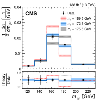
Figure 1: CMS benchmark result from Ref. [30]. It shows the differential top pair cross section as a function of the top-jet invariant mass, compared to theory predictions for different top masses. The vertical bars represent the total uncertainties, statistical uncertainties are shown as short horizontal bars, and theoretical uncertainties as shaded bands.

Once we have measured the top mass in an event sample, we can further analyse the unfolded dataset. For instance, we can look for effects from higher-dimensional SMEFT operators on the decay of boosted tops, or we can search for anomalous kinematic distributions from new particles, modified interactions, or enhanced QCD effects at the subjet level. While the unfolding for the top mass measurement has to include a sufficiently large number of dimensions, as discussed above, we now need to unfold the full, 12-dimensional phase space. Three of these dimensions are finite jet masses, generated by QCD effects.

2.2 Dataset

We use simulated events for top pair production, similar to the one used for the CMS jet mass measurement [30]. We generate the events with Madgraph 5 [31]. Hadronization, parton showers, and multiple parton interactions are simulated with Pythia8.230 [32] with the underlying event tune CP5. The samples include a simulation of the detector response implemented in Delphes 3.5.0 [33] using the default CMS card with pile-up, and the e-flow algorithm. The pile-up subtraction only removes charged tracks associated to pile-up vertices.

In the simulated data, we have access to three stages of the simulation chain. particles. The parton level includes the hard interactions of the top quarks, that decay into a $b$-quark and a $W$-boson, that subsequently decays into two quarks or lepton and neutrino. The particle level refers to all stable particles with lifetimes longer than $10^{-8}$ s after parton shower and hadronization. Finally, the detector level describes particle candidates after the detector simulation.

Event selections are applied at the particle and detector level. All events that do not pass any of the selections are rejected from the further analysis. For the signal or measurement region, we only consider lepton-hadron top pairs at the parton level,

$$pp\to t\bar{t}\to(bq\bar{q}^{\prime})\;(\bar{b}\ell^{-}\bar{\nu})+\text{c.c.}\quad\text{with}\quad\ell=e,\mu\;,$$ (1)

and the lepton acceptance

$$p_{T,\ell}>60\;\text{GeV}\quad\text{and}\quad|\eta_{\ell}|<2.4\;.$$ (2)

The top jet is constructed using XCone clustering and identified by the larger angular distance to the lepton and must fulfill

$$p_{T,J}>400\;\text{GeV}\qquad\text{and}\qquad p_{T,j_{1,2,3}}>30\;\text{GeV}\qquad|\eta_{j_{1,2,3}}|<2.5\;,$$ (3)

for the fat jet $J$ and three subjets $j$. In the following, we will refer to these subjets as jets. The second jet has to have $p_{T}>10\;\text{GeV}$ to reject poorly reconstructed events. To reduce the contribution from events where not the full top quark decay is reconstructed within the fat jet, we require the invariant mass of the three jets, $M_{jjj}$, to exceed the invariant mass of the second jet and the lepton.

At the detector level, we require missing transverse momentum above $50\;\text{GeV}$ and at least one $b$-tagged jet.

The measurement-region selection criteria leaves us with approximately 700,000 events simulated with a top mass of $m_{t}=172.5\;$\mathrm{G}\mathrm{e}\mathrm{V}$$, of which we use 75% for training. To be consistent with the amount of available full detector simulations at CMS, we chose samples with different top masses to have a factor of 10 less events. All events contain the full gen-level and reco-level kinematic information. The XCone algorithm clusters the jets separately for reco-level jets and gen-level jets. The clustered jets are sorted according to $p_{T}$.

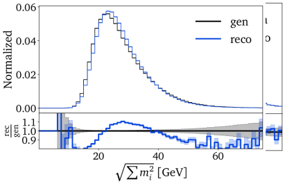
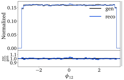
Figure 2: Kinematic distributions at reco-level and gen-level for the second jet (top), combining two jets (center), and combining three jets (bottom).

2.3 Jet-mass features

For the generative unfolding algorithm a perfect matching between reco-level and gen-level jets is not critical, as the reco-level is used only as a condition. We have checked that when permuting the ordering of the reco-level jets randomly, we observe no difference in performance. Once we switch to the 4-momentum representation ($m,p_{T},\phi,\eta$), we see small differences between reco-level and gen-level, for instance in the jet masses shown in Fig. 2.

Differences in the jet masses are mostly due to pile-up, which in our simulation is added at reco-level. Events are to some degree corrected by removing tracks originating from pile-up vertices. The remaining difference in the jet mass mostly comes from neutral hadrons in the pile-up. This positive contribution to the jet masses is largest for the leading jet because of its largest $p_{T}$. Figure 2 implies that unfolding detector effects includes unfolding these pile-up effects. As Delphes assumes idealized vertex reconstruction, we expect those differences to be larger when including full detector effects with GEANT4 [34].

Going beyond single-jet observables, we need to understand and eventually unfold detector effects on correlations. In Fig. 2 we show a few examples. For the angular separation of the two leading jets the peak is generated by the boosted decay kinematics combined with mass effects and the detector acceptance. The 2-jet masses have a peculiar distribution, owed to the fact that out of the three jets two come from the $W$-decay. Because of the $p_{T}$-ordering, any of the three combinations

$$M_{ik}^{2}=m_{i}^{2}+m_{k}^{2}+2\;\left(m_{T,i}m_{T,k}\cosh{\Delta\eta_{ik}}-p_{T,i}p_{T,k}\cos{\Delta\phi_{ik}}\right)$$ (4)

can reconstruct $m_{W}$. This is an exact equation for the three 2-jet masses, if $\Delta\eta_{ik}$ is calculated using the jet rapidities. Of the three 2-jet masses in a top decay, two tend to be similarly close to $M_{ik}\sim m_{W}$ [35]. In Fig. 2 we also observe the upper endpoint in the top decay kinematics at gen-level [36]

$$m_{bj}^{\text{max}}<\sqrt{m_{t}^{2}-m_{W}^{2}}\approx 155\leavevmode\nobreak\ \text{GeV}\;.$$ (5)

Following Eq.(4) we can improve the training of the unfolding network by including the 2-jet masses as explicit features. Each of the 2-jet masses then substitutes an angular variable. With this basis transformation we sacrifice access to the individual azimuthal angles and are left with their absolute differences.

Next, we see in Fig. 2 that the transverse top momentum is not affected significantly by the detector effects, and the 3-jet mass peaks at the top mass value. In our phase space parametrization we can calculate the 3-jet mass as

$$M_{jjj}^{2}=M_{12}^{2}+M_{23}^{2}+M_{13}^{2}-m_{1}^{2}-m_{2}^{2}-m_{3}^{2}$$ (6)

By using all these jet masses as training features, we can greatly improve the learning and unfolding of the 3-jet mass. The no-free-lunch theorem, however, tells us that this gain will lead to a mis-modelling of other correlations. In particular, we will see that there is no guarantee that $\cos{\Delta\phi}\in[0,1]$ anymore, leading to the generation of unphysical event kinematics in some cases.

2.4 Generative unfolding

Traditional unfolding algorithms [37, 38, 39] have been used to unfold simple differential cross section measurements. Widely used methods include Iterative Bayesian Unfolding [40, 41, 42, 43], Singular Value Decomposition [44], and TUnfold [45]. Their limitation is the need for binned data over low-dimensional phases space. This also means that we have to pre-select the observables we want to unfold and their binning.

To use ML-methods for high-dimensional and unbinned unfolding, we invert the forward simulation using Bayes’ theorem

$$p(x_{\text{gen}}|x_{\text{reco}})=p(x_{\text{reco}}|x_{\text{gen}})\;\frac{w(x_{\text{gen}})p(x_{\text{gen}})}{w(x_{\text{reco}})p(x_{\text{reco}})}\;,$$ (7)

where $x_{\text{gen}}$ is a point in the weighted gen-level phase space and $x_{\text{reco}}$ a point in the weighted reco-level phase space. To unfold reco-level data, we need to learn

$$p_{\text{model}}(x_{\text{gen}}|x_{\text{reco}})\approx p(x_{\text{gen}}|x_{\text{reco}})$$ (8)

as the statistical basis of an inverse simulation. Once a generative neural network encodes $p_{\text{model}}(x_{\text{gen}}|x_{\text{reco}})$, we calculate

$$p_{\text{unfold}}(x_{\text{gen}})=\int dx_{\text{reco}}\;p_{\text{model}}(x_{\text{gen}}|x_{\text{reco}})w(x_{\text{reco}})p(x_{\text{reco}})\;.$$ (9)

At the event level, this integral can easily be evaluated by marginalizing the corresponding joint probability. Our method can be summarized as

$$p_{\text{sim}}(x_{\text{gen}}) p_{\text{unfold}}(x_{\text{gen}})$$

$$\hskip-25.60747pt\text{\footnotesize paired data}\Bigg{\updownarrow} \hskip 17.07164pt\Bigg{\uparrow}{\scriptstyle p_{\text{model}}(x_{\text{gen}}|x_{\text{reco}})}$$

$$p_{\text{sim}}(x_{\text{reco}})\quad\xleftrightarrow{\text{\; correspondence \;}}\quad p_{\text{data}}(x_{\text{reco}})$$ (10)

The two distributions $p_{\text{sim}}(x_{\text{reco}})$ and $p_{\text{sim}}(x_{\text{gen}})$ are encoded in one set of simulated events, before and after detector effects, or at the parton-level and at reco-level.

Figure 3: Schematic representation of generative unfolding with a CFM network.

The generative network we employ to learn $p_{\text{model}}(x_{\text{gen}}|x_{\text{reco}})$ is Conditional Flow Matching (CFM). The generative CFM network is the leading architecture for precision-LHC simulations [23]. Mathematically, CFM is based on two equivalent ways of describing a diffusion process using am ODE or a continuity equation [46]

$$\frac{dx(t)}{dt}=v(x(t),t)\qquad\text{or}\qquad\frac{\partial p(x,t)}{\partial t}=-\nabla_{\theta}\left[v(x(t),t)p(x(t),t)\right]\;,$$ (11)

both with the same velocity field $v(x(t),t)$. The diffusion process described by $t\in[0,1]$ relates a Gaussian $r$-distribution to the physical phase space $x$,

$$p(x,t)\to\begin{cases}p_{\text{data}}(x)\qquad\quad&t\to 0\\ p_{\text{latent}}(r)=\mathcal{N}(r;0,1)\qquad\quad&t\to 1\;,\end{cases}$$ (12)

We employ a simple linear interpolation

$$x(t) =(1-t)x+tr\to\begin{cases}x\qquad\quad&t\to 0\\ r\sim\mathcal{N}(0,1)\qquad\quad&t\to 1\;.\end{cases}$$ (13)

Using this approximation, we train the network to learn

$$v_{\theta}(x(t),t)\approx v(x(t),t)$$ (14)

using the continuity equation, and then generate phase space configurations using a fast ODE solver. Even though the corresponding MSE loss function

$$\mathcal{L}_{\text{CFM}}=\left[w(x)(v_{\theta}-(r-x))\right]^{2}$$ (15)

is not a likelihood loss, a Bayesian version of the CFM generative network can learn uncertainties on the underlying phase space density together with the central values underlying its sampling [23].

The CFM setup is illustrated in Fig. 3. Its conditional extension is straightforward, in complete analogy to the conditional GANs [12] and conditional INNs [13] developed for unfolding. While the naive GAN setup does not learn the event-wise (inverse) migration correctly and therefore does not encode physical, calibrated conditional probabilities, the cINN with its likelihood loss does exactly that. The CFM succeeds because of its mathematical foundation, Eq.(11) [3].

Training bias

In Eq.(10) we describe the structure of generative unfolding, but we are missing a critical complication — the simulated reco-level data $p_{\text{sim}}(x_{\text{reco}})$ might not agree with the actual reco-level data $p_{\text{data}}(x_{\text{reco}})$. Let us assume a simple case where the simulation depends on a simulation parameter $m_{s}$ which we can tune to describe the actual data. This can be a physics parameter we eventually infer, or a nuisance parameter which we profile over. The dependencies of the four datasets on $m_{s}$ and its ‘correct’ value in the data, $m_{d}$, turn Eq.(10) into

$$p_{\text{sim}}(x_{\text{gen}}|m_{s}) p_{\text{unfold}}(x_{\text{gen}}|m_{s},m_{d})$$

$$\hskip-25.60747pt{\scriptstyle p(x_{\text{reco}}|x_{\text{gen}})}\Bigg{\downarrow} \hskip 17.07164pt\Bigg{\uparrow}{\scriptstyle p_{\text{model}}(x_{\text{gen}}|x_{\text{reco}},m_{s})}$$

$$p_{\text{sim}}(x_{\text{reco}}|m_{s})\quad\xleftrightarrow{\text{\; correspondence \;}}\quad p_{\text{data}}(x_{\text{reco}}|m_{d})$$ (16)

In the forward direction, $p(x_{\text{reco}}|x_{\text{gen}})$ does not have an explicit $m_{s}$-dependence, but both simulated datasets follow $p_{\text{sim}}(x_{\text{gen}}|m_{s})$ and $p_{\text{sim}}(x_{\text{reco}}|m_{s})$ induced by the generator settings. By assumption, $m_{s}=m_{d}$ ensures that the simulated and actual data agree at the reco-level,

$$p_{\text{sim}}(x_{\text{reco}}|m_{s}=m_{d})\stackrel{{\scriptstyle!}}{{=}}p_{\text{data}}(x_{\text{reco}}|m_{d})\;.$$ (17)

We then use this relation to infer $m_{d}$ at the reco-level.

Alternatively, we can do the same inference at the gen-level, requiring

$$p_{\text{sim}}(x_{\text{gen}}|m_{s}=m_{d})\stackrel{{\scriptstyle!}}{{=}}p_{\text{unfold}}(x_{\text{gen}}|m_{s}=m_{d},m_{d})\;.$$ (18)

The problem with this unfolded inference is the dual dependence of $p_{\text{unfold}}(x_{\text{gen}}|m_{s},m_{d})$ through the reco-level data and the learned conditional probability. This dual dependence is automatically resolved if $p_{\text{unfold}}(x_{\text{gen}})$ only depends on $m_{d}$ through the reco-level data, so the bias from $p_{\text{model}}(x_{\text{gen}}|x_{\text{reco}},m_{s})$ can be neglected. If not, we can use iterative methods [15] to remove the bias. The iterative improvement relies on a learned classifier over $x_{\text{gen}}$ which reweights $p_{\text{sim}}$ to $p_{\text{unfold}}$ including the $m_{s}$-dependencies and serves as a basis for re-training the unfolding network. It implicitly assumes that $p_{\text{unfold}}(x_{\text{gen}}|m_{s},m_{d})$ depends mostly on $m_{d}$ and at a reduced level on $m_{s}$. In that case the endpoint of the Bayesian iteration is reached when the two dependencies coincide at the level of the remaining statistical uncertainty.

3 Unbinned top decay unfolding

Unfolding top decays is technically challenging, because the top mass and the $W$-mass are dominant features over an altogether 12-dimensional phase space. We start with a naive unfolding in Sec. 3.1, using our appropriate phase space parametrization with reduced dimensionality [17]. In Sec. 3.2, we show how the model dependence from the top mass in the training data can be controlled. With this improvement, we show in Sec. 3.3 how the high-dimensional unfolding can improve the existing top mass measurement using classic unfolding. Finally, we show how to unfold the entire 12-dimensional phase space using the measured top mass in Sec. 3.4.

3.1 Lower-dimensional unfolding

We know that the precision of learned phase space distribution using neural networks scales unfavorably with the phase space dimension [47, 48]. The full 12-dimensional phase space will not be the optimal representation to measure the top mass. Instead, we only use a lower-dimensional phase space representation for the top mass measurement, finding a balance between relevant kinematic information and dimensionality. We postpone the full kinematic unfolding to the point where we need to access to the full kinematics and benefit from the measured top mass

For the traditional CMS analysis [30], two phase space dimensions were unfolded, $M_{jjj}$ and $p_{T,jjj}$. A jet energy calibration relies on the reconstructed $W$-boson. Identifying the $W$-decay jets in the top ideally requires $b$-tagging information, which is not available in our case. Without $b$-tagging, our goal is to calibrate jets using as much reliable jet information as possible. From Fig. 2 we know that all 2-jet masses include a sharp $W$-mass peak, suggesting that we unfold those for the top mass measurement.

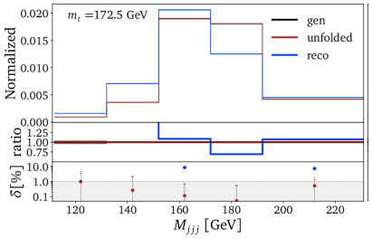
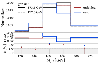
Figure 4: Kinematic distributions from 4-dimensional unfolding. We also show the reco-level and the gen-level truth for $m_{t}=172.5$ GeV. In the bottom-right panel we compare $M_{jjj}$ for $m_{t}=172.5$ GeV to generated unfolding for $m_{t}=173.5$ GeV, not seen during training.

Our unfolding setup follows Sec. 2.3. From Eq.(6) we know that we can extract the 3-jet mass as a proxy for the top mass from the set of single-jet and 2-jet masses. Because the single-jet masses are largely universal and not a good handle on the jet energy calibration, our first choice is to measure the top mass from a 4-dimensional unfolding of

$$\Big{\{}\;M_{j1j2},M_{j2j3},M_{j1j3},\sum_{i}m_{i}\;\Big{\}}\;.$$ (19)

The results are shown in Fig. 4. First, we see that we can unfold the sum of the single jet masses extremely well, with deviations of the unfolded data from the generator truth at the per-cent level. This means that we expect to be able to extract the 3-jet mass essentially from the sum of all 2-jet masses with a known and controlled offset.

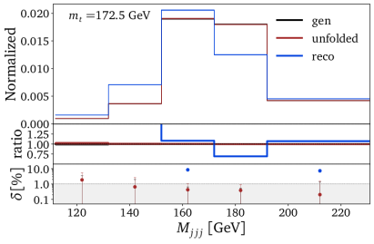
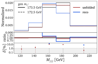
Figure 5: Kinematic distributions from 6-dimensional unfolding. In the right panel we compare $M_{jjj}$ for $m_{t}=172.5$ GeV to generated unfolding for $m_{t}=173.5$ GeV, not seen during training.

Next, we show a 2-jet mass, with the characteristic $W$-peak and the shoulder at $m_{bj}^{\text{max}}$. The $W$-peak is washed out at the reco-level, but the generative unfolding reproduces it extremely well. The relative deviation of the unfolded to the truth 2-jet mass distributions is at most a few per-cent, with no visible shift around the $W$-peak. The same quality of the unfolding can be observed in the $M_{jjj}$ distribution, perfectly reproducing the top mass at $m_{t}=172.5$ GeV, the correct value in the training data and in the data which gets unfolded.

The problem with measuring the top mass from unfolded data appears when we unfold data simulated with a different top mass. In the lower-right panel of Fig. 4 we show the unfolded $M_{jjj}$ distribution for reco-level data generated with $m_{t}=173.5$ GeV, unfolded with generative networks trained on $m_{t}=172.5$ GeV. We see that the top peak in the unfolded data is dominated by the training bias of the network, specifically a maximum at $M_{jjj}=(172\pm 1)$ GeV. This means the top peak is entirely determined by the training bias and hardly impacted by the reco-level data which we unfold.

From the 4-dimensional unfolding we know that the network learns the $W$-peak in the 2-jet masses and the top peak in the 3-jet mass at a precision much below the physical particle widths. The problem is that the bias from the network training completely determines the position of these mass peaks in the unfolded data. To confirm that these findings are not an artifact of our reduced phase space dimensionality, we repeat the same analysis for the 6-dimensional phase space

$$\Big{\{}\;M_{j1j2},M_{j2j3},M_{j1j3},m_{j1},m_{j2},m_{j3}\;\Big{\}}\;.$$ (20)

The unfolded 3-jet mass distributions are shown in Fig. 5, corresponding to the 4-dimensional case in Fig. 4. While the unfolded peak in $M_{jjj}$ is a slight bit worse than for the easier 4-dimensional case, the bias from the training remains, in spite of the fact that we are weakening the expressive power of the unfolding network by adding distributions that are mildly affected by the peak position.

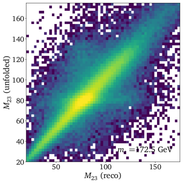
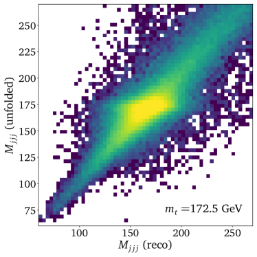
Figure 6: Truth and learned migration in the $M_{jjj}$ distribution between reco-level and gen-level.

Finally, we can look at the truth and learned migration between the reco-level and the gen-level 3-jet distribution in Fig. 6. In the left panel we see that the forward simulation maps the sharp peak at gen-level to a broader peak at reco-level. The problem with the central ellipse describing this physical migration by detector effects is that it does not indicate any correlation between the $M_{jjj}$-values at reco-level and at gen-level. The learned migration in the right panel reproduces the forward migration exactly.

For the generative unfolding this means that small differences at reco-level will always be unfolded to the same sharp region at gen-level, independent of the information contained in the reco-level data. Following Sec. 2.4 and Eq.(16) the unfolded distribution $p_{\text{unfold}}(x_{\text{gen}})$ is entirely determined by the training choice $m_{s}$ and shows practically no dependence on the value $m_{d}$ encoded in the actual data.

3.2 Taming the training bias

The next question is how we can improve the situation where, $m_{s}$ being the top mass value used for the simulation and $m_{d}$ the actual top mass in the data, Eq.(16) turns into

$$p_{\text{sim}}(x_{\text{gen}}|m_{s}) p_{\text{unfold}}(x_{\text{gen}}|m_{s},\cancel{m_{d}})$$

$$\hskip-25.60747pt{\scriptstyle p(x_{\text{reco}}|x_{\text{gen}})}\Bigg{\downarrow} \hskip 17.07164pt\Bigg{\uparrow}{\scriptstyle p_{\text{model}}(x_{\text{gen}}|x_{\text{reco}},m_{s})}$$

$$p_{\text{sim}}(x_{\text{reco}}|m_{s})\quad\xleftrightarrow{\text{\; correspondence \;}}\quad p_{\text{data}}(x_{\text{reco}}|m_{d})$$ (21)

In the unfolded distribution the training information $m_{s}$ completely overwrites $m_{d}$. Moreover, even if there was enough sensitivity, a classifier comparing two shifted mass peaks learns weights far away from unity, leading to numerical challenges. This means we cannot use the usual iterative methods to remove the bias from the training data.

Following the strategy from Sec. 2, we first increase the sensitivity on $m_{d}$. For this, we pre-process the data such that $m_{d}$ is directly accessible by adding an estimator of $m_{d}$ to the representation of $x_{\text{reco}}$. Ideally, this estimator would be inspired by an optimal observable. Such a 1-dimensional sufficient statistics should exist, and we know how to construct it. For the top mass we just use the weighted median of the 3-jet masses at reco-level, $M_{jjj}^{\text{batch}}$. For a batch size around $10^{4}$ events, this information will be strongly correlated with the top mass,

$$M_{jjj}^{\text{batch}}\approx m_{d}\equiv m_{t}\Bigg{|}_{\text{data}}\;.$$ (22)

This batch-wise kinematic information can be extracted at the level of the loss evaluation, and it goes beyond the usual single-event information, similar to established MMD loss modifications of GAN training [21, 12].

Second, we weaken the bias from the training data by combining training data with different top masses, but without an additional label,

$$m_{t}=\left\{169.5,172.5,175.5\right\}\leavevmode\nobreak\ \text{GeV}\qquad\quad\text{(combined training).}$$ (23)

It turns out sufficient to cover a range of top masses with separate, unmixed training batches. The range ensures that top masses in the actual data are within the range of the training data. We ensure a balanced training by enlarging the event samples with $m_{t}=169.5$ GeV and $m_{t}=175.5$ GeV to match the size of the largest sample. This is done by repeating and shuffling the input data, which effectively uses these events several times per epoch. With an appropriate regularization we avoid overfitting. The limited number of CMS simulated events for the eventual analyses makes this training strategy sub-optimal. We expect larger and additional $m_{t}$ simulations, unavailable at this time, to improve the results. We observed that both steps need to be included to ensure precise, unbiased results.

Obviously, this strategy of strengthening the dependence on $m_{d}$ and reducing the training bias is not applicable to all problems, and it does not lead to the endpoint of the Bayesian iterative method, but for our combined inference-unfolding strategy it works, and this is all we need.

Transfusion architecture

Figure 7: Schematic representation of a parallel transfusion network, adapted from [3].

As the network task becomes significantly more difficult we replace the simple dense architecture with a transfusion network, described in detail in Ref. [51, 3] and visualized in Fig. 7.

Each component of the $n$-dimensional condition as well as of the time-dependent $N$-dimensional input $x(t)$ are individually embedded by concatenating positional information and zero padding. The embedded conditions are passed through the encoder part of a transformer, while the embedded input is passed through the decoder counterpart. In both transformer parts, we apply self-attention to learn the correlations in the condition and in the input. It is complemented by a cross-attention between encoder and decoder outputs, to learn the correlations between conditions and inputs. They are crucial for the unfolding task. The transformer outputs for every component of the input one high-dimensional embedding vector $c_{i}$, which is mapped back to a 1-dimensional component of the velocity field by a shared dense linear network. This way we express the learned $N$-dimensional velocity field of Eq.(14) as

$$v_{\theta}(x_{\text{gen}}(t),t,x_{\text{reco}})=\left(v_{\theta}(c_{1},t),\dots,v_{\theta}(c_{N},t)\right).$$ (24)

The hyperparameters of the network can be found in Appendix A.

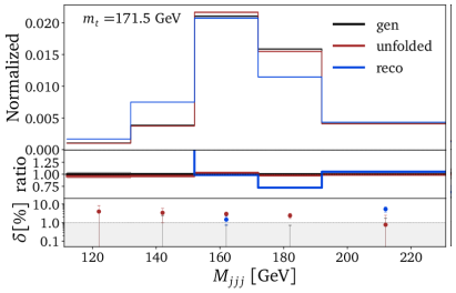
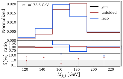
Figure 8: $M_{jjj}$-distribution from 4-dimensional unfolding of data with $m_{t}=171.5$ GeV (left) and $m_{t}=173.5$ GeV (right). We train the network combining samples with three top masses, Eq.(23).

Using the transfusion network we unfold the 4-dimensional phase space from Eq.(19). The results are shown in Fig. 8. We unfold data generated with two different top masses, $m_{t}=171.5$ GeV and $m_{t}=173.5$ GeV. Neither of these two values are present in the training data. In both panels we see that the top mass as the main kinematic feature is reproduced well, without a significant effect in the relative deviation. The fitted peak values of the distribution are $m_{\text{peak}}=(172\pm 1)$ GeV when unfolding data with 171.5 GeV, and $m_{\text{peak}}=(174\pm 1)$ GeV when unfolding data 173.5 GeV. While the bias might not have vanished entirely, it is well contained within the numerical uncertainties. We will extract the unfolded top mass value properly in Sec. 3.3.

Dual network

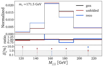
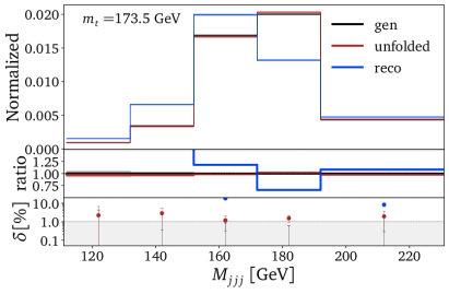
Figure 9: Unfolded $M_{jjj}$ with two networks from 6-dimensional unfolding of data with $m_{t}=171.5$ GeV (left) and $m_{t}=175.5$ GeV (right). We train the network combining samples with three top masses, Eq.(23).

Given the more complicated training task, we observe a drop in performance when we increase the dimensionality to unfold the 6-dimensional phase space

$$x=\big{(}\;\{m_{i}\},\{M_{ik}\}\big{)}\;,$$ (25)

defined in Eq.(20) using the transfusion network. Inspired by Refs. [22, 23], we factorize the phase space density into two parts, each encoded in a generative network: the first network learns the individual jet mass directions in phase space, which are universal and do not depend on the value of $m_{t}$; a second network generates the 2-jet masses conditioned on the individual jet masses,

$$p(x_{\text{gen}}|x_{\text{reco}})=\underbrace{p\left(\{m_{i,\text{gen}}\}\big{|}\;x_{\text{reco}},M_{jjj}^{\text{batch}}\right)}_{\text{network 1}}\underbrace{p\left(\{M_{ik,\text{gen}}\}\big{|}\;\{m_{i,\text{gen}}\},x_{\text{reco}},M_{jjj}^{\text{batch}}\right).}_{\text{network 2}}$$ (26)

Both CFM-transfusion networks also receive $M_{jjj}^{\text{batch}}$ calculated for a full batch using Eq.(6). For the event generation we first generate the unfolded jet masses $\{m_{i}\}$, pass them as a condition to the second network, and then generate the unfolded 2-jet masses $\{M_{ik}\}$.

Looking at the 6-dimensional correlation giving $M_{jjj}$ in Fig. 9, we observe a hardly visible drop in performance, but still no bias from the training data. As before we observe peak values at $m_{\text{peak}}=(172\pm 1)$ GeV when unfolding data with 171.5 GeV and at $m_{\text{peak}}=(174\pm 1)$ GeV when unfolding data with 173.5 GeV.

3.3 Mock top mass measurement

We estimate the benefit from generative unfolding by repeating the top mass measurement from Ref. [30], but with a large number of bins in the $M_{jjj}$ histogram. The top mass is extracted from the binned unfolded distributions using a fit based on $\chi^{2}=d^{T}V^{-1}d$, where $d$ is the vector of bin-wise differences between the normalized unfolded distribution and the normalized prediction from the simulated data. The covariance matrix $V$ contains the uncertainties and corresponding bin-to-bin correlations. A parabola fit provides the central value of $m_{t}$ and the standard deviation.

Statistical and model uncertainties

First, this fit requires the covariance matrix describing statistical uncertainties [52]. We sample from the latent space, conditional on the reco-level events, $N$ times, which means we generate $N$ unfolded distributions from the posterior $p_{\text{model}}(x_{\text{gen}}|x_{\text{reco}})$. We then use a Poisson bootstrap, where we assign a weight from a Poisson distribution with unit mean. The size of one replica is 52,000 events, corresponding to the approximate number of real data events. The number of events follows a Poisson distribution, with the mean given by the nominal sample size.

For the measurement, we create $N_{\text{rep}}=1000$ replicas by selecting the nominal number of reco-level events from the test dataset with $m_{t}=172.5$ GeV and the full datasets for the simulations at different top masses. We unfold each replica, calculate $M_{jjj}$, and use the histogram entries $u_{i}^{(n)}$ to compute the correlation matrix of statistical fluctuations as

$$\text{cov}_{ij} =\frac{1}{N_{\text{rep}}}\sum_{n=1}^{N_{\text{rep}}}(u_{i}^{(n)}-\bar{u}_{i})(u^{(n)}_{j}-\bar{u}_{j})\qquad\text{with}\qquad\bar{u}_{i}=\frac{1}{N_{\text{rep}}}\sum_{n=1}^{N_{\text{rep}}}u^{(n)}_{i}$$

$$\text{corr}_{ij} =\frac{\text{cov}_{ij}}{\sqrt{\text{cov}_{ii}}\sqrt{\text{cov}_{jj}}}\;.$$ (27)

This procedure also takes into account the uncertainties due to the statistical fluctuations of $M_{jjj}^{\text{batch}}$. The training of the network itself introduces correlations which are at least one order of magnitude smaller and therefore ignored in the measurement.

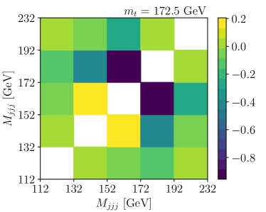
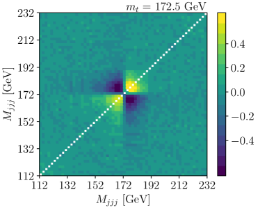
Figure 10: Correlation matrices for $m_{t}=172.5$ GeV from $N_{\text{rep}}=1000$ replicas in 60 bins (right) and 5 bins (left) for the 4-dimension unfolding.

The $60\times 60$ correlation matrix for the 4-dimensional unfolding using the largest sample generated with $m_{t}=172.5$ GeV is shown in Fig. 10. We see two distinct source of bin-to-bin correlations. In general, an event migrating from bin $i$ to bin $j$ gives rise to negative correlations in the number of events between the two bins. Additionally, unbiasing the unfolding ensures that a shift in the batch-wise condition also shifts the unfolded peak. This effect, accounted for in the bootstrapping method, introduces an additional contribution to the bin-to-bin correlations. It causes positive correlations between bins on the same side of the peak and anti-correlations otherwise. In our case, both effects are most apparent in the peak region and its neighbouring bins as shown in Fig. 10. Second, we follow Ref. [30] to estimate the uncertainty from the choice of $m_{t}$ in the simulation. We evaluate the difference between the unfolded distribution and the corresponding simulated gen-level distribution for each bin and construct a covariance matrix

$$\text{cov}_{ij}=\sigma_{i}\rho_{ij}\sigma_{j}\;,$$ (28)

where $\sigma_{i}$ is the uncertainty in bin $i$, and $\rho_{ij}$ the correlation between bins $i$ and $j$. These bin-to-bin correlations are not known, but since we do not observe any systematic pattern, we neglect the bin-to-bin correlations and use a diagonal covariance matrix. It was verified that other choices do not alter the results. To estimate the impact of this model uncertainty, we perform the $m_{t}$ extraction twice. First, we only include the statistical covariance matrix corresponding to 52,000 available events at the reco-level. Second, we repeat the same measurement also including the model uncertainty.

Improvement

Figure 11: Extraction of $m_{t}$ with a $\chi^{2}$ test only accounting for statistical uncertainties and with the additional model uncertainty from the choice of $m_{t}$ in the simulation.

To compare our new unfolding technique to the existing TUnfold results [30], we repeat the extraction using the simulated data sets with 172.5 GeV and using the statistical covariance matrix from the measured data, published in HEPData [53]. The $\chi^{2}$-curves and the corresponding results are displayed in Fig. 11, where we show the 4-dimensional and 6-dimensional unfoldings with 60 bins and the TUnfold result. We see that the uncertainty in the choice of $m_{t}$ is reduced from being a leading model uncertainty in the CMS measurement to a negligible level as well as a reduction in the statistical uncertainty due to the finer binning.

To confirm that the choice in $m_{t}$ does not leave a residual bias, we repeat the top quark mass extraction for different top masses in the reco-level data. The results are shown in the left panel of Fig. 12. For a top mass of $m_{t}=173.5$\mathrm{G}\mathrm{e}\mathrm{V}$$ we observe a bias when looking at the fit using 5 bins. This is not surprising as the exact binning has been fine tuned for the extraction of $m_{t}$ using the CMS full simulation and hence it is not optimal for our analysis. Nevertheless, while the bin width in the unfolding with TUnfold is limited by the jet mass resolution, we test various binning schemes for the unbinned unfolding and observe closure for up to 30 bins. For finer binnings the resolution is too fine for the comparably coarse grid of available gen-level distributions with $m_{t}=\{169.5,171.5,172.5,173.5,175.5\}\;\text{GeV}$, leading to an unstable closure test altogether.

Circumventing this limitation, we interpolate the gen-level distributions for $m_{t}$-values close to $172.5$ GeV, where three samples with a separation of 1 GeV are available and a linear dependence of the bin content on $m_{t}$ is a valid approximation. Now, we can compare the generative unfolding with 5 to 60 bins in terms of the statistical uncertainty. The results are displayed in the right panel of Fig. 12, indicating an increase in the precision of the top mass due to the improved resolution.

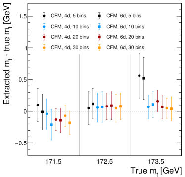
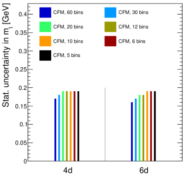
Figure 12: Left: deviation of the extracted top mass from the reco-level truth, employing 4-dimensional and 6-dimensional unfolding for the assumed values of $171.5,172.5$, and $173.5$ GeV. Right: statistical uncertainties of the extractions of the top mass from the 4-dimensional and 6-dimensional unfolding with different binnings, assuming $m_{t}=172.5$ GeV.

3.4 Full phase space unfolding

As a last step of our unfolding program, we need to unfold the full 12-dimensional phase space given the measured top mass. This has the advantage that the leading source of training bias is removed. Following the same precision arguments as before, we keep the mass basis of Eq.(20) for the first 6 of the 12 phase space dimensions. This ensures that the 2-jet and 3-jet masses are reproduced well, albeit not at the level of the dedicated first unfolding step.

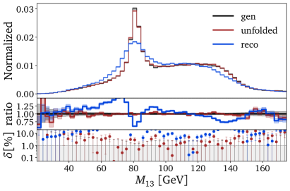
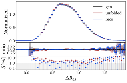
Figure 13: Kinematic distributions from full, 12-dimensional unfolding. We show the 3-jet mass as well as the azimuthal angle between the two leading jets.

The remaining phase space dimensions are

$$x=\big{(}\;\{m_{i}\},\{M_{ik}\},\{p_{T,i}\},\{\eta_{i}\}\;\big{)}\qquad i,k=1,2,3\;,$$ (29)

all other kinematic observables can be computed from these basis directions. For the 12-dimensional unfolding we use a single transfusion network, after checking that the dual network does not lead to an improvement. The hyperparameters are given in Appendix A.

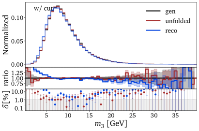
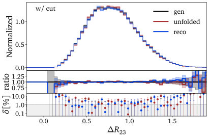
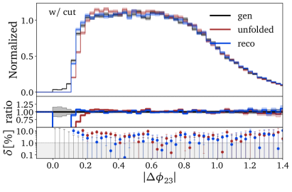
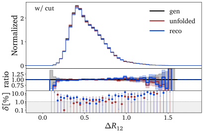
Figure 14: Kinematic distributions from full, 12-dimensional unfolding. We show the target 3-jet distribution, the azimuthal angle between the jets after cut, and a set of single-jet observables, 2-jet correlations, and 3-jet correlations (top to bottom).

Two kinematic distributions are shown in Fig 13. In the left panel we see that the top mass peak is learned almost as well as for the 4-dimensional and 6-dimensional cases. Indeed, this is the case for all jet masses and 2-jets masses, which are combined to the 3-jet mass with the top peak.

A serious issue arises from the azimuthal angle between the two leading jets, $|\Delta\phi_{ik}|$. According to Eq.(4) this angle is learned as a correlations of 7 phase space directions. Moreover, we do not have access to the azimuthal angles, only to the cosine of differences between angles. Here the problem arises that the network does not ensure that this cosine comes out in the physical range $-1\leavevmode\nobreak\ ...\leavevmode\nobreak\ 1$. We enforce the physical range by clipping the cosine for small angles to one, which causes a mis-modelling of the small-$|\Delta\phi_{ik}|$ regime, shown in the right panel of Fig. 14.

A simple way to improve this mis-modelling is to require $\cos\Delta\phi_{12}<1$. However, from Fig. 13 we know that this does not solve the problem. Instead, we accept the fact that for unfolding the masses well we might have to pay a prize in the coverage of the angular correlations, and we apply an additional acceptance cut

$$\Delta\phi_{ik}>0.1$$ (30)

both, at the reco- and gen-levels of the unfolded events. This reduces the unfolded dataset by 30%. An extended set of unfolded kinematic distribution after this cut are shown in Fig 14.

We know that our unfolding methods covers correlations between the original phase space directions well, because many of the kinematic observables shown in Fig 14 are, in reality, complex correlations of our phase space basis. However, to end with a nice figure and to drive home the message that high-dimensional unfolding using conditional generative networks does learn the corresponding correlations well, we show one of our favorite correlations in Fig 15. Indeed, there is literally no difference in the correlation between two of the three 2-jet masses. This correlation also confirms that the condition $M_{ik}\approx m_{W}$ leads to three distinct lines in phase space, where close to the crossing points it is impossible to reconstruct which of the two jets come from the $W$-decay.

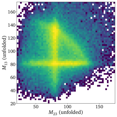
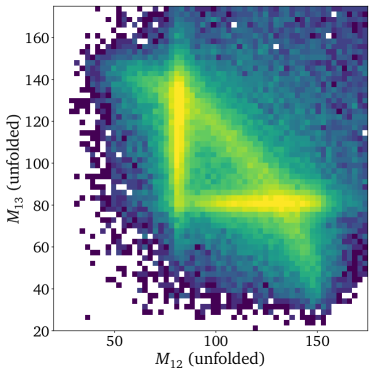
Figure 15: Correlation of two 2-jet masses at gen-level truth (left) and after unfolding (right).

4 Outlook

Unfolding is one of the ways modern machine learning is transforming the way we can do LHC physics. Employing an inverse simulation, it allows us to analyze LHC extremely efficiently within the LHC collaborations, to combine analyses between different experiments, and even make data accessible to experts outside the experimental collaborations. Unfolding has been used in particle physics frequently, but modern neural networks allow us to unfold high-dimensional phase spaces without binning. This technical advance can turn unfolding into a standard analysis method for LHC experiments.

For our study, we unfold detector effects from boosted top decay data using state-of-the-art conditional generative networks. Unfolding decay kinematics is especially challenging because we expect a large model dependence and even systematic bias from the choice of the top mass in the simulated training data. Our study shows that generative unfolding can solve this problem and provides a first milestone towards incorporating generative unfolding in an existing LHC analysis.

First, we showed that for an appropriate phase space parametrization, a combination of diffusion network and transformer can reliably unfold a 4-dimensional and 6-dimensional subspace of the full top-decay phase space at the percent level precision. This included the 3-jet mass as a proxy to the top mass. The problem in this unfolding is a strong bias from the top mass used to generate the training data. To compensate this bias we added a global estimate of the top mass to the representation of the measured data and weakened the training bias by including a range of top masses there. As a result of these two structural modifications, the top mass bias was essentially removed.

Using this setup we showed how to extract the top mass along the lines of the CMS analysis in Ref. [30]. We included two covariance matrices, one describing all statistical uncertainties and one covering the model uncertainty from the training data. We found that, indeed, the impact of the model uncertainty is becoming irrelevant, and that the error on the top mass extraction can be reduced when using the kind of fine binning allowed by the unbinned unfolding method.

Finally, we unfolded the full, 12-dimensional phase space for a given top mass. One failure mode in reproducing the angular distributions was induced by our phase space parametrization. However, a simple lower cutoff on the azimuthal angle separations of the top decay jets allowed for an excellent reproduction of all correlations.

This study is meant to serve as a blueprint for an actual CMS analysis, both, for a top mass measurement and for a wider use of the unfolded data.

Appendix A Hyperparameters

Parameter
LR sched.	cosine
Max LR	$10^{-3}$
Optimizer	Adam
Batch size	16384
Network	Resnet
Dim embedding	64
Intermediate dim	512
Num layers	8

Table 1: Parameters for the 4-dimensional and 6-dimensional networks in Sec. 3.1.

Parameter	4D	6D
Epochs	800	$500(+1000)$
LR sched.	cosine	cosine
Max LR	$10^{-3}$	$10^{-3}$
Optimizer	Adam	Adam
Batch size	10000	10000
Dropout	0.1	0.1
Network	Transfusion	Transfusion
Dim embedding	64	64
Intermediate dim	512	512
Num layers	4	4
Num heads	4	4

Table 2: Parameters for the 4-dimensional and 6-dimensional networks in Sec. 3.2.

Parameter	12D
Epochs	500
LR sched.	cosine
Max LR	$10^{-3}$
Optimizer	Adam
Batch size	16384
Dropout	0.1
Network	Transfusion
Dim embedding	128
Intermediate dim	512
Num layers	6
Num heads	4

Table 3: Parameters for the 12-dimensional network in Sec. 3.4.

References

- [1] J. M. Campbell et al., Event Generators for High-Energy Physics Experiments, in Snowmass 2021. 3, 2022. arXiv:2203.11110 [hep-ph].
- [2] S. Badger et al., Machine learning and LHC event generation, SciPost Phys. 14 (2023) 4, 079, arXiv:2203.07460 [hep-ph].
- [3] N. Huetsch et al., The Landscape of Unfolding with Machine Learning, arXiv:2404.18807 [hep-ph].
- [4] A. Andreassen, P. T. Komiske, E. M. Metodiev, B. Nachman, and J. Thaler, OmniFold: A Method to Simultaneously Unfold All Observables, Phys. Rev. Lett. 124 (2020) 18, 182001, arXiv:1911.09107 [hep-ph].
- [5] LHCb, R. Aaij et al., Multidifferential study of identified charged hadron distributions in -tagged jets in proton-proton collisions at 13 TeV, Phys. Rev. D 108 (2023) L031103, arXiv:2208.11691 [hep-ex].
- [6] ATLAS, G. Aad et al., A simultaneous unbinned differential cross section measurement of twenty-four +jets kinematic observables with the ATLAS detector, arXiv:2405.20041 [hep-ex].
- [7] K. Datta, D. Kar, and D. Roy, Unfolding with Generative Adversarial Networks, arXiv:1806.00433 [physics.data-an].
- [8] J. N. Howard, S. Mandt, D. Whiteson, and Y. Yang, Learning to simulate high energy particle collisions from unlabeled data, Sci. Rep. 12 (2022) 7567, arXiv:2101.08944 [hep-ph].
- [9] S. Diefenbacher, G.-H. Liu, V. Mikuni, B. Nachman, and W. Nie, Improving generative model-based unfolding with Schrödinger bridges, Phys. Rev. D 109 (2024) 7, 076011, arXiv:2308.12351 [hep-ph].
- [10] A. Butter, T. Jezo, M. Klasen, M. Kuschick, S. Palacios Schweitzer, and T. Plehn, Kicking it Off(-shell) with Direct Diffusion, arXiv:2311.17175 [hep-ph].
- [11] A. Butter, S. Diefenbacher, N. Huetsch, V. Mikuni, B. Nachman, S. Palacios Schweitzer, and T. Plehn, Generative Unfolding with Distribution Mapping, arXiv:2411.02495 [hep-ph].
- [12] M. Bellagente, A. Butter, G. Kasieczka, T. Plehn, and R. Winterhalder, How to GAN away Detector Effects, SciPost Phys. 8 (2020) 4, 070, arXiv:1912.00477 [hep-ph].
- [13] M. Bellagente, A. Butter, G. Kasieczka, T. Plehn, A. Rousselot, R. Winterhalder, L. Ardizzone, and U. Köthe, Invertible Networks or Partons to Detector and Back Again, SciPost Phys. 9 (2020) 074, arXiv:2006.06685 [hep-ph].
- [14] M. Vandegar, M. Kagan, A. Wehenkel, and G. Louppe, Neural Empirical Bayes: Source Distribution Estimation and its Applications to Simulation-Based Inference, arXiv:2011.05836 [stat.ML].
- [15] M. Backes, A. Butter, M. Dunford, and B. Malaescu, An unfolding method based on conditional Invertible Neural Networks (cINN) using iterative training, arXiv:2212.08674 [hep-ph].
- [16] M. Leigh, J. A. Raine, K. Zoch, and T. Golling, -flows: Conditional neutrino regression, SciPost Phys. 14 (2023) 6, 159, arXiv:2207.00664 [hep-ph].
- [17] J. Ackerschott, R. K. Barman, D. Gonçalves, T. Heimel, and T. Plehn, Returning CP-Observables to The Frames They Belong, arXiv:2308.00027 [hep-ph].
- [18] A. Shmakov, K. Greif, M. Fenton, A. Ghosh, P. Baldi, and D. Whiteson, End-To-End Latent Variational Diffusion Models for Inverse Problems in High Energy Physics, arXiv:2305.10399 [hep-ex].
- [19] A. Shmakov, K. Greif, M. Fenton, A. Ghosh, P. Baldi, and D. Whiteson, Full Event Particle-Level Unfolding with Variable-Length Latent Variational Diffusion, arXiv:24xx.xxxxx [hep-ex].
- [20] A. Butter, S. Diefenbacher, G. Kasieczka, B. Nachman, and T. Plehn, GANplifying event samples, SciPost Phys. 10 (2021) 6, 139, arXiv:2008.06545 [hep-ph].
- [21] A. Butter, T. Plehn, and R. Winterhalder, How to GAN LHC Events, SciPost Phys. 7 (2019) 6, 075, arXiv:1907.03764 [hep-ph].
- [22] A. Butter, T. Heimel, S. Hummerich, T. Krebs, T. Plehn, A. Rousselot, and S. Vent, Generative networks for precision enthusiasts, SciPost Phys. 14 (2023) 4, 078, arXiv:2110.13632 [hep-ph].
- [23] A. Butter, N. Huetsch, S. Palacios Schweitzer, T. Plehn, P. Sorrenson, and J. Spinner, Jet Diffusion versus JetGPT – Modern Networks for the LHC, arXiv:2305.10475 [hep-ph].
- [24] R. Das, L. Favaro, T. Heimel, C. Krause, T. Plehn, and D. Shih, How to understand limitations of generative networks, SciPost Phys. 16 (2024) 1, 031, arXiv:2305.16774 [hep-ph].
- [25] K. Danziger, T. Janßen, S. Schumann, and F. Siegert, Accelerating Monte Carlo event generation – rejection sampling using neural network event-weight estimates, SciPost Phys. 12 (9, 2022) 164, arXiv:2109.11964 [hep-ph].
- [26] T. Janßen and S. Schumann, Machine learning efforts in Sherpa, J. Phys. Conf. Ser. 2438 (2023) 1, 012144.
- [27] T. Heimel, R. Winterhalder, A. Butter, J. Isaacson, C. Krause, F. Maltoni, O. Mattelaer, and T. Plehn, MadNIS - Neural multi-channel importance sampling, SciPost Phys. 15 (2023) 4, 141, arXiv:2212.06172 [hep-ph].
- [28] T. Heimel, N. Huetsch, F. Maltoni, O. Mattelaer, T. Plehn, and R. Winterhalder, The MadNIS Reloaded, arXiv:2311.01548 [hep-ph].
- [29] T. Heimel, O. Mattelaer, T. Plehn, and R. Winterhalder, Differentiable MadNIS-Lite, arXiv:2408.01486 [hep-ph].
- [30] CMS, A. Tumasyan et al., Measurement of the differential production cross section as a function of the jet mass and extraction of the top quark mass in hadronic decays of boosted top quarks, Eur. Phys. J. C 83 (2023) 7, 560, arXiv:2211.01456 [hep-ex].
- [31] J. Alwall, R. Frederix, S. Frixione, V. Hirschi, F. Maltoni, O. Mattelaer, H. S. Shao, T. Stelzer, P. Torrielli, and M. Zaro, The automated computation of tree-level and next-to-leading order differential cross sections, and their matching to parton shower simulations, JHEP 07 (2014) 079, arXiv:1405.0301 [hep-ph].
- [32] T. Sjöstrand, S. Ask, J. R. Christiansen, R. Corke, N. Desai, P. Ilten, S. Mrenna, S. Prestel, C. O. Rasmussen, and P. Z. Skands, An introduction to PYTHIA 8.2, Comput. Phys. Commun. 191 (2015) 159, arXiv:1410.3012 [hep-ph].
- [33] DELPHES 3, J. de Favereau, C. Delaere, P. Demin, A. Giammanco, V. Lemaître, A. Mertens, and M. Selvaggi, DELPHES 3, A modular framework for fast simulation of a generic collider experiment, JHEP 02 (2014) 057, arXiv:1307.6346 [hep-ex].
- [34] R. Brun, F. Bruyant, F. Carminati, S. Giani, M. Maire, A. McPherson, G. Patrick, and L. Urban, GEANT Detector Description and Simulation Tool, .
- [35] T. Plehn, M. Spannowsky, M. Takeuchi, and D. Zerwas, Stop Reconstruction with Tagged Tops, JHEP 10 (2010) 078, arXiv:1006.2833 [hep-ph].
- [36] T. Plehn and M. Takeuchi, W+Jets at CDF: Evidence for Top Quarks, J. Phys. G 38 (2011) 095006, arXiv:1104.4087 [hep-ph].
- [37] G. Cowan, A survey of unfolding methods for particle physics, Conf. Proc. C 0203181 (2002) 248.
- [38] F. Spano, Unfolding in particle physics: a window on solving inverse problems, EPJ Web Conf. 55 (2013) 03002.
- [39] M. Arratia et al., Publishing unbinned differential cross section results, JINST 17 (2022) 01, P01024, arXiv:2109.13243 [hep-ph].
- [40] L. B. Lucy, An iterative technique for the rectification of observed distributions, The Astronomical Journal 79 (June, 1974) 745.
- [41] W. H. Richardson, Bayesian-based iterative method of image restoration, J. Opt. Soc. Am. 62 (Jan, 1972) 55.
- [42] L. B. Lucy, An iterative technique for the rectification of observed distributions, Astron. J. 79 (1974) 745.
- [43] G. D’Agostini, A Multidimensional unfolding method based on Bayes’ theorem, Nucl. Instrum. Meth. A362 (1995) 487.
- [44] A. Hocker and V. Kartvelishvili, SVD approach to data unfolding, Nucl. Instrum. Meth. A372 (1996) 469, arXiv:hep-ph/9509307 [hep-ph].
- [45] S. Schmitt, TUnfold: an algorithm for correcting migration effects in high energy physics, JINST 7 (2012) T10003, arXiv:1205.6201 [physics.data-an].
- [46] T. Plehn, A. Butter, B. Dillon, T. Heimel, C. Krause, and R. Winterhalder, Modern Machine Learning for LHC Physicists, arXiv:2211.01421 [hep-ph].
- [47] D. Maître and H. Truong, A factorisation-aware Matrix element emulator, JHEP 11 (7, 2021) 066, arXiv:2107.06625 [hep-ph].
- [48] S. Badger, A. Butter, M. Luchmann, S. Pitz, and T. Plehn, Loop amplitudes from precision networks, SciPost Phys. Core 6 (2023) 034, arXiv:2206.14831 [hep-ph].
- [49] J. Spinner, V. Bresó, P. de Haan, T. Plehn, J. Thaler, and J. Brehmer, Lorentz-Equivariant Geometric Algebra Transformers for High-Energy Physics, arXiv:2405.14806 [physics.data-an].
- [50] J. Brehmer, V. Bresó, P. de Haan, T. Plehn, H. Qu, J. Spinner, and J. Thaler, A Lorentz-Equivariant Transformer for All of the LHC, arXiv:2411.00446 [hep-ph].
- [51] T. Heimel, N. Huetsch, R. Winterhalder, T. Plehn, and A. Butter, Precision-Machine Learning for the Matrix Element Method, arXiv:2310.07752 [hep-ph].
- [52] M. Backes, A. Butter, M. Dunford, and B. Malaescu, Event-by-event Comparison between Machine-Learning- and Transfer-Matrix-based Unfolding Methods, arXiv:2310.17037 [physics.data-an].
- [53] CMS Collaboration, “Measurement of the jet mass distribution and top quark mass in hadronic decays of boosted top quarks in proton-proton collisions at = 13 TeV.” HEPData (collection), 2023. https://doi.org/10.17182/hepdata.130712.