Ensemble control of n-level quantum systems with a scalar control
Abstract
In this paper we discuss how a general bilinear finite-dimensional closed quantum system with dispersed parameters can be steered between eigenstates. We show that, under suitable conditions on the separation of spectral gaps and the boundedness of parameter dispersion, rotating wave and adiabatic approximations can be employed in cascade to achieve population inversion between arbitrary eigenstates. We propose an explicit control law and test numerically the sharpness of the conditions on several examples.
1 Introduction
Let us consider a continuum of -level closed quantum systems described by the Schrödinger equation
| (1) |
where is a real-valued control. Here the Hamiltonian is determined by an unknown parameter taking values in a closed and connected subdomain of . We assume that has the structure
where is a continuous function for each . The matrix is self-adjoint and describes the control coupling between the eigenstates of the system. It has the form
where the are real parameters. We assume that each is unknown but that it belongs to some closed interval in . We are going to consider the ensemble control problem consisting in steering the continuum of dynamics (1) with the same control signal, independent of and of the .
Our main tool to tackle the problem is the adiabatic theory which states that, for a slowly varying Hamiltonian, the spectral subspaces are approximately invariant under the associated dynamics (see [18]).
The problem of ensemble controllability for quantum systems has been mainly developed for two-level systems steered by two real-valued controls. In experimental situations it is often takled via direct optimization methods (see, for instance, [5, 8] and also the review papers [7, 10]). The mathematical aspects of the ensemble controllability problem have been addressed, in particular, in [4, 12, 13]. In these papers the authors show that a uniform control can be constructed to steer the system from a common initial state to an arbitrary set of target states continuously parameterized by the uncertainties of the system, i.e., . Let us also mention [1, 2, 11] for some further results on ensemble control of quantum systems by adiabatic motion and [6, 15] for related ensemble stabilization problems for two-level quantum systems. For systems with a single scalar input, as described in system (1), the strategies used in the papers above cannot be applied directly due to the lack of degrees of freedom. In the physics literature, the most common way to approximate an effective Hamiltonian with several degrees of freedom using a single input is through the rotating wave approximations. However, this approach is not always compatible with the ensemble adiabatic motion, as observed in [16]. The article [16] proposes a rigorous constructive approach that combines, in a suitable range of dispersion parameters, rotating wave and adiabatic approximations, extending the results for 2-level systems [4, 12, 13] to the case of scalar controls. Results for the ensemble control of -level systems with a scalar input have been obtained in [3]. The latter article uses a different combination of adiabatic and rotating wave approximations, which is robust with respect to coupling strengths in but not to dispersions in the frequencies of . Up to now the problem of ensemble control of a -level systems with a scalar control with dispersions in the frequencies of remained open. This is what we are studying in the present paper by extending the approach developed in [16]. The analysis is here much more complicated since the presence of several energy levels increases the possible resonances.
We employ the rotating wave approximation and an adiabatic approximation in cascade to realise population inversion between an arbitrary pair of eigenstates of . High-order averaging results are necessary in both the rotating wave and adiabatic steps. Otherwise the fidelity of their cascade can fail to converge to 1 due to the competing time scales of the two approximations. We highlight the importance of having no overlaps between the uncertainty intervals of each frequency and that, assuming further higher-order conditions on the resonance frequencies, it is possible to steer the system with higher precision.
The article is organized as follows: In Section 2, we state the main result (Theorem 1) and we provide an explicit construction of the control law. We provide a sketch of the main steps of the proof of Theorem 1 in Section 3. The proof itself is given in Section 4, where fast-oscillating terms are first eliminated through successive time-dependent changes of variables and rotating wave approximations. A non-standard adiabatic theorem is then applied to the system. In Section 5, we test numerically the sharpness of the proposed conditions in the case of a 4-level system.
2 Results
To realize a population inversion between two arbitrary eigenstates, we will consider a time scale for the rotating wave approximation and another time scale for the adiabatic following. The control law in our algorithm will be a chirped pulse of the type
| (2) |
where are functions to be chosen. The goal is to induce a transition from the initial state towards a state of the form in time when and are small.
In the following, we will denote by the canonical basis of and the canonical basis of (space of real matrices).
Theorem 1.
Let us assume that for all , and for all , . Fix . Assume that belongs to a closed interval such that and there exist such that
-
1.
For all , ;
-
2.
For all such that and all , we have .
Fix and take such that
-
i)
and ;
-
ii)
and .
Denote by the solution of (1) with initial condition and the control law as in (2). Then there exist and such that for every and every ,
for some .
Remark 2.
If we choose , then there exists such that for every and ,
that is, the final state is arbitrarily close to the eigenstate , up to a phase, as goes to zero.
Remark 3.
Here we fix and give a simple construction of the control law satisfying the conditions of Theorem 1 by choosing and for . Thus the control law is given by
for all .
With a stronger assumption on eigenvalues of the system, we obtain a better estimation of the error. A preliminary version of this result on three-level systems has been proposed in [14].
Proposition 4.
Assume that the assumptions of Theorem 1 are satisfied, and moreover, for all and , . Then there exist and such that for every ,
3 Sketch of the proof
The proof of Theorem 1 consists of the following steps:
- •
-
•
Step 2: Hypothesis 2 of Theorem 1 allows us to introduce the change of variables in equation (10) to eliminate all oscillating terms of order except for the term with time-dependent frequency that couples the pair . Due to the non-linearity of the dynamics, this first-order elimination generates new oscillating terms of order .
-
•
Step 3: We show that, thanks to Hypothesis 2 of Theorem 1, the oscillating term with frequency introduces an implicit rotation between . This rotation is characterized by the radius and the angle , as defined in equations (21) and (22). In equation (24), a change of variables is introduced to recast the dynamics in a rotational frame depending on and .
-
•
Step 4: Using higher-order averaging results, we introduce the change of variables in equation (37) to eliminate all oscillating terms of order .
-
•
Step 5: In Lemma 17, we obtain an approximate dynamics by truncating the residual term of the Hamiltonian. This truncation and the earlier steps correspond to the rotating wave approximation (RWA).
-
•
Step 6: We project the approximate dynamics onto the two-dimensional subspace and apply a non-standard adiabatic approximation to achieve population inversion between and in the approximate dynamics.
-
•
Step 7: Finally, we conclude the proof by combining the errors from the rotating wave approximation (Steps 1-5) and the adiabatic approximation (Step 6).
4 Proof of Theorem 1
Step 1: Interaction frame
Define . In the following, we will replace by , which will only introduce a relative phase to the state. Moreover, this transition will not change the gaps between eigenvalues, the system will always satisfy the conditions in Theorem 1, and For and , let us define
| (3) | ||||
Let us fix . For , define
| (4) |
Let us recast (1) in the interaction frame . Notice that
| (5) |
where
For and , let us define
| (6) | ||||
Notice that by definition of in equation (3), for all , . Then, when applying the chirped pulse given in (2), we obtain
| (7) |
Step 2: First-order elimination
In the following proposition, we give the expansion of the Hamiltonian after a general unitary change of variables.
Proposition 5 (Change of variables).
Consider the change of variables , where is a smooth curve in the space of Hermitian matrices and is the solution of the Schrödinger equation
Then is the solution of
| (8) |
where is given by
Proof.
By differentiating , we can deduce that the dynamics of is characterized by the Hamiltonian
By the Baker–Campbell–Hausdorff formula and by Theorem 4.5 in [9], we have
Hence, we conclude that
∎
Definition 6.
Fix , we call a -parameterized function if for every , is a real-valued function defined on . Given an -parameterized function and , we say that over if there exist such that for every and , we have .
Let us first define the sets of indices
| (9) |
By Hypothesis 2 of Theorem 1 and the assumptions made on , for every and , , where is introduced in equation (6). Then we can apply a first change of variables to system (5) , where
| (10) |
Notice that, for every , and over , where is defined in Definition 6. Then, by differentiating , we obtain that
| (11) |
By Proposition 5, we deduce that the dynamics of are characterized by the Hamiltonian
By equations (7) and (11), we obtain that
| (12) |
over . For , let us define
Notice that when , for every , we have and . For and let us note, for every ,
Then, we obtain the following notations
and
We can deduce from equation (12) that
| (13) |
over , where
| (14) |
and, for every and ,
Step 3: Implicit rotation between
Set
| (15) |
Since by the assumption of Theorem 1, we have and for all , we can deduce that, for every and , . Let us introduce a second change of variables , where
| (16) |
Notice that
over . Then, by Proposition 5 and Equation (13), we deduce that, over , the dynamics of are characterized by the Hamiltonian
Remark 7.
Since , we deduce that for every . Then and . Hence, and .
Notice that . Let us introduce a third change of variables, namely, , where
| (17) |
Let us define
| (18) |
Then the dynamics of are characterized by the Hamiltonian
where
| (19) |
and
| (20) | ||||
For and , let us define
| (21) | ||||
| (22) |
where is the sign of .
Remark 8.
By definition of and , it follows that, for ,
Moreover, the assumptions on and given in Theorem 1 ensure that and .
Lemma 9.
.
Proof.
Since in (2) is strictly increasing on , let us define the function such that
| (23) |
Lemma 10.
There exist and such that, for all , .
The proof of the lemma can be found in the appendix.
Remark 11.
In the following, for simplicity of notation, we will denote and simply as and . Notice that .
Step 4: Second-order elimination
Let us define , and introduce the change of variables , where
| (24) | ||||
The dynamics of are characterized by the Hamiltonian
| (25) | ||||
Here is given in equation (20), is given by
| (26) | ||||
where is defined in equation (4) and
| (27) |
is given by
| (28) | ||||
where
| (29) | ||||
and, finally, is given by
| (30) | ||||
where
| (31) | ||||
The proof of the following three lemmas can be found in the appendix.
Lemma 12.
For , given two smooth functions and , define , where is defined as in (22). Then there exist and such that for all and , .
Lemma 13.
Lemma 14.
There exists such that, for all and , .
In the proofs of the following lemmas, we are going to apply the adaptations of the classical Van der Corput lemma (see for example [17]) to quantum systems proposed in [2].
Lemma 15.
over .
Proof.
Take . By the change of variables , we have
| (32) |
By Lemma 12, there exist and such that for all and , we have . Notice that, by equation (4) and hypotheses of Theorem 1, we have . Then by equation (32) and Corollary A.7 in [2], we can deduce that there exists such that, for all and ,
Then by equation (32) and the definition of in equation (3), we obtain that, for all ,
| (33) |
over Take . By the change of variables ,
| (34) |
Notice that by Lemma 13. By the assumptions of Theorem 1, for all . By applying Corollary A.6 in [2] with and Lemma 12 to equation (LABEL:eq:int_function_2), we can prove that, over ,
Notice that, by Lemma 13, there exists such that, for all , we have . Then by a reasoning similar to that above, we can prove that, over ,
Then by the definition of in equation (3), we have that, over ,
| (35) |
By definition of in equation (27), we deduce that . Similarly, we can obtain that, over ,
| (36) |
By equations (33), (35), and (36), we can conclude the proof. ∎
Lemma 16.
Over ,
Proof.
Notice that for all and . Then by the same reasoning as that in the proof of Lemma 15, we obtain that, over .
Step 5: Rotating wave approximation
Let us introduce the truncation of given by
We denote by the solution of
| (40) |
Lemma 17.
over .
Proof.
Introduce the -valued functions and solutions of , with initial conditions , . It is evident that and for every . By differentiating with respect to , we obtain that
Then over , we have that
By Lemma 10 and equation (39), there exist and such that, for , we have that, over ,
Notice that for all . Then we can deduce that, over ,
and
∎
For ], define the unitary transformation
| (41) |
where and are given as in changes of variables (17) and (24). Then, let us introduce the following change of variables that pushes the truncated system backward to the original frame:
The initial state of is and its dynamics are characterized by the Hamiltonian
| (42) |
Recall that for .
Lemma 18.
For , we have
Proof.
By Remark 7, we have
| (43) |
On the other hand, for all , we have
Since, by definition (41), is unitary and for all , we deduce that
| (44) |
By equations (37), (38), and (40), we have that and . Then . By equations (37), (39), and Lemma 17, we have and . The conclusion follows from equations (43) and (44). ∎
Step 6: Non-standard adiabatic approximation
For a system characterized by the Hamiltonian given in equation (42), it is evident that the dynamics in the two-dimensional space are decoupled from the rest of the system. Let us define the decoupled Hamiltonian. Let us introduce the decoupled Hamiltonian
By assumptions of Theorem 1 and the change of variables in equation (5), is in the two-dimensional space . By Lemma 18, and . Then the solution of
satisfies
| (45) |
We can then apply Lemma 30 in [16] to the decoupled 2-level system and obtain that, for the control given in Theorem 1, there exist and such that, for and ,
Step 7: Combination of rotating wave and adiabatic approximations
By equation (45) and Lemma 18, there exist and such that, for and ,
By the change of variables (5), it follows that there exist and such that, for and ,
Proof of Proposition 4.
Under the same assumption as in Theorem 1, we introduce a change of variables as in equation (10) where the dynamics are characterized by the Hamiltonian given in equation (13). Define the set
| (46) |
where is defined in equation (14). The additional assumptions of Proposition 4 ensure that, for every ,
Then we introduce the following change of variables:
where
Since for every , we have . Therefore and . By Proposition 5, the dynamics of are characterized by the Hamiltonian
Then we introduce the truncation of given by
Denote by the solution of
| (47) |
Using a similar reasoning as in the proof of Lemma 17, we prove that . Then by adiabatic following argument similar to that in the proof of Theorem 1, we conclude that there exist and such that, for and ,
∎
5 Example
Consider the four-level system with drift and control Hamiltonians
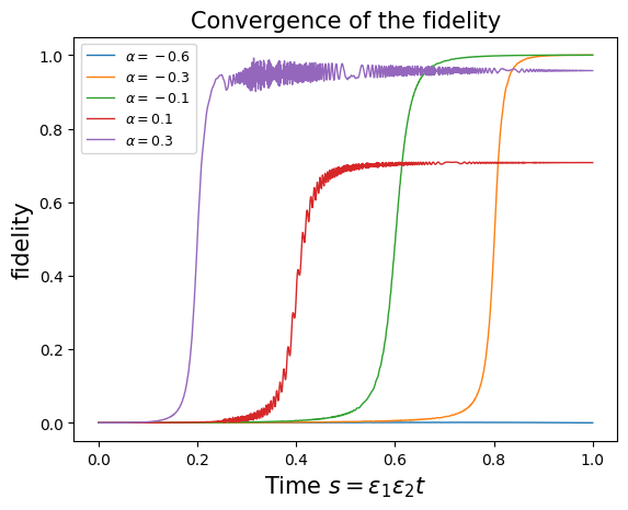
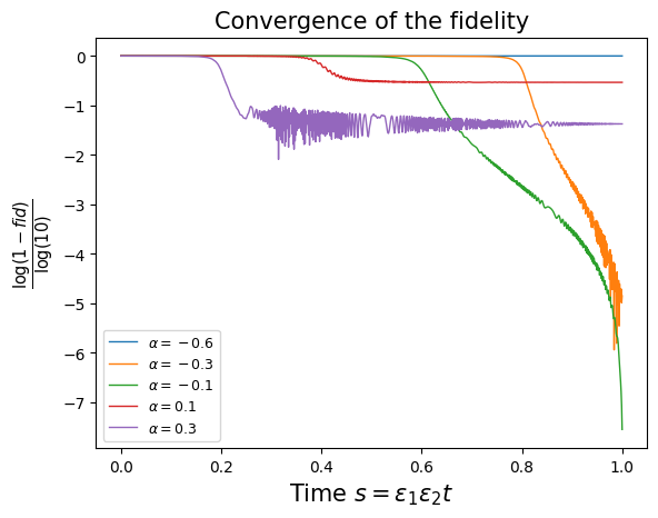
Fix the initial state . In order to realize a population inversion between the third and the forth eigenstates, let us fix and use the control law given in Remark 3 with . We will test the sharpness of conditions for . We are going to use the time scale . For , let us define the fidelity of the inversion as the population on the target state at instant :
Here the target state is . When or , falls in the open interval , and for with , is not in the closed interval . When , is not in , violating the hypothesis 1 of Theorem 1. When or , falls in the closed interval and the hypothesis 2 of Theorem 1 is violated. See the results in Figure 1.
Finally, let us test if it is possible to realize a population inversion between and by successive inversions between , between , and between . Notice that a direct inversion between and is impossible since . Fix for this test. To realize the inversion between and , let us choose and construct a control law defined on as described in Remark 3. It can be easily verified that the assumptions in Theorem 1 are satisfied. Similarly, we choose to construct for the inversion between and to construct for the inversion between . A concatenation of these three control laws, defined on , is given by
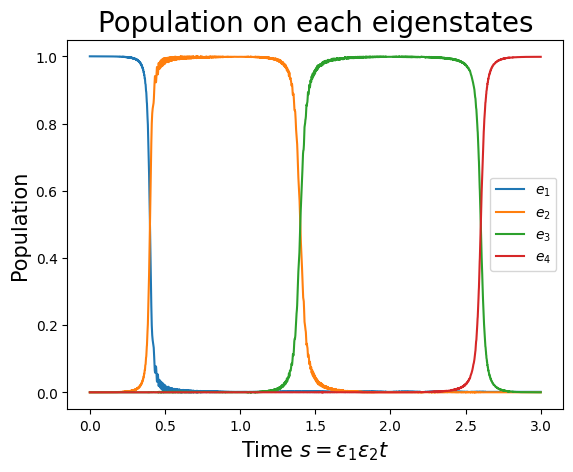
The numerical result is given in Figure 2 with the time scale , showing the efficiency of the algorithm.
6 Conclusion
In this study, we introduced an algorithm capable of realizing population inversion between two arbitrary eigenstates for a continuum of quantum systems. We underlined the importance of the non-overlapping condition on some characteristic frequencies for this algorithm’s validity. Future investigations could explore the possibility of proposing weaker conditions for convergence, extending similar results to infinite-dimensional quantum systems and examining which further controllability results (i.e. population splitting) could be obtained in addition to population inversion.
7 Appendix
Proof of Lemma 10.
By the definition of in 22, we have that
| (48) |
The conditions on and in Theorem 1 ensure that there exist and such that , for all , and for all . Then, by equation (48), we deduce that for all . Since does not change sign on , we obtain that
For all , by equation (21), we have . Then by equation (48), we deduce that there exists such that for all . Therefore,
We conclude that there exist and such that, for all , we have . ∎
Proof of Lemma 12.
For and , we have
By Lemma 10, there exists such that, for all , . We can conclude the proof by choosing . ∎
Proof of Lemma 13.
By equation (21),
Take . By the definition of in (23) and the assumption of Theorem 1 on , we have and . Then, we can easily deduce that
Take . By equation (21) and triangle inequality, we have that
Since on , we can deduce that
By the assumptions of Theorem 1, there exists such that for all . We conclude the proof by choosing . ∎
Acknowledgments
This work has been partly supported by the ANR-DFG project “CoRoMo” ANR-22-CE92-0077-01. This project has received financial support from the CNRS through the MITI interdisciplinary programs.
References
- [1] Nicolas Augier, Ugo Boscain, and Mario Sigalotti. Adiabatic ensemble control of a continuum of quantum systems. SIAM J. Control Optim., 56(6):4045–4068, 2018.
- [2] Nicolas Augier, Ugo Boscain, and Mario Sigalotti. Semi-conical eigenvalue intersections and the ensemble controllability problem for quantum systems. Math. Control Relat. Fields, 10(4):877–911, 2020.
- [3] Nicolas Augier, Ugo Boscain, and Mario Sigalotti. Effective adiabatic control of a decoupled hamiltonian obtained by rotating wave approximation. Automatica, 136:110034, 2022.
- [4] Karine Beauchard, Jean-Michel Coron, and Pierre Rouchon. Controllability issues for continuous-spectrum systems and ensemble controllability of Bloch equations. Comm. Math. Phys., 296(2):525–557, 2010.
- [5] Chunlin Chen, Daoyi Dong, Ruixing Long, Ian R Petersen, and Herschel A Rabitz. Sampling-based learning control of inhomogeneous quantum ensembles. Physical Review A, 89(2):023402, 2014.
- [6] Francesca C. Chittaro and Jean-Paul Gauthier. Asymptotic ensemble stabilizability of the Bloch equation. Systems Control Lett., 113:36–44, 2018.
- [7] S. J. Glaser, U. Boscain, T. Calarco, C. P. Koch, W. Köckenberger, R. Kosloff, I. Kuprov, B. Luy, S. Schirmer, T. Schulte-Herbrüggen, D. Sugny, and F. K. Wilhelm. Training Schrödinger’s cat: quantum optimal control. Strategic report on current status, visions and goals for research in Europe. European Physical Journal D, 69:279, 2015.
- [8] Steffen J Glaser, Ugo Boscain, Tommaso Calarco, Christiane P Koch, Walter Köckenberger, Ronnie Kosloff, Ilya Kuprov, Burkhard Luy, Sophie Schirmer, Thomas Schulte-Herbrüggen, et al. Training schrödinger’s cat: Quantum optimal control: Strategic report on current status, visions and goals for research in europe. The European Physical Journal D, 69:1–24, 2015.
- [9] Brian C. Hall. An elementary introduction to groups and representations, 2000.
- [10] Christiane P Koch, Ugo Boscain, Tommaso Calarco, Gunther Dirr, Stefan Filipp, Steffen J Glaser, Ronnie Kosloff, Simone Montangero, Thomas Schulte-Herbrüggen, Dominique Sugny, et al. Quantum optimal control in quantum technologies. strategic report on current status, visions and goals for research in europe. EPJ Quantum Technology, 9(1):19, 2022.
- [11] Z. Leghtas, A. Sarlette, and P. Rouchon. Adiabatic passage and ensemble control of quantum systems. Journal of Physics B, 44(15), 2011.
- [12] Jr-Shin Li and Navin Khaneja. Ensemble controllability of the Bloch equations. In Proceedings of the 45th IEEE Conference on Decision and Control, pages 2483–2487. IEEE, 2006.
- [13] Jr-Shin Li and Navin Khaneja. Ensemble control of Bloch equations. IEEE Transactions on Automatic Control, 54(3):528–536, 2009.
- [14] Ruikang Liang, Ugo Boscain, and Mario Sigalotti. Ensemble quantum control with a scalar input. In Proceedings of the 63rd IEEE Conference on Decision and Control. IEEE, 2024.
- [15] Ulisses Alves Maciel Neto, Paulo Sergio Pereira da Silva, and Pierre Rouchon. Motion planing for an ensemble of Bloch equations towards the south pole with smooth bounded control. Automatica J. IFAC, 145:Paper No. 110529, 9, 2022.
- [16] Rémi Robin, Nicolas Augier, Ugo Boscain, and Mario Sigalotti. Ensemble qubit controllability with a single control via adiabatic and rotating wave approximations. Journal of Differential Equations, 318:414–442, 2022.
- [17] Elias M Stein and Timothy S Murphy. Harmonic analysis: real-variable methods, orthogonality, and oscillatory integrals, volume 3. Princeton University Press, 1993.
- [18] Stefan Teufel. Adiabatic perturbation theory in quantum dynamics, volume 1821 of Lecture Notes in Mathematics. Springer-Verlag, Berlin, 2003.