Extending the Leader-First Follower Structure for Bearing-only Formation Control on Directed Graphs

Abstract

This work proposes an extension to the leader-first follower (LFF) class of graphs used to solve the bearing-only formation control problem over directed graphs. The first contribution provides an equilibrium, stability, and convergence analysis for a one-follower, multi-leader system (which is not an LFF graph). We then propose an extension to the LFF structure, termed ordered LFF graphs, that allows for additional forward directed edges to be included. Using the results of the one-follower multi-leader system we show that the ordered LFF graphs can be used to solve the directed bearing-only formation control problem. We also show that these structures offer improved convergence speed as compared to the LFF graphs. Numerical simulations are provided to validate the results.

I INTRODUCTION

Formation control has obtained significant attention across a wide range of fields, including robotics [1], aerial and ground vehicle networks [2], and swarm robotics [3]. The primary task in formation control is to drive a team of autonomous systems into a desired spatial configuration. As a cornerstone problem in multi-agent coordination, one of the challenges in formation control is the design of distributed control protocols that balance the sparsity of information exchange with the performance of the system. In this direction, there is a considerable body of literature that addresses this problem for a variety of different formation and sensing constraints. These include position-constrained formation control [4], displacement-constrained formation control [5], distance-constrained formation control [6], bearing-constrained formation control [7], and most recently angle-constrained formation control [8]. The reader is referred to [9, 10, 11] for an overview of this area.

Despite recent progress in the study of formation control problems, there remains a large gap between the theoretical advances and their real-world implementation. Indeed, many works on multi-agent systems assume undirected communication and sensing networks. In reality, sensing employed in, for example, robotic systems is inherently uni-directional. In other words, if agent $i$ can sense agent $j$, it is not necessarily true that agent $j$ can sense agent $i$. The problem of directed formation control was originally studied by Hendrickx et. al in [12] where the notion of persistence was introduced to describe consistency in directed distance-constraint frameworks. This work however did not consider formation control strategies for directed frameworks, but rather attempted to characterize the feasibility sets of directed frameworks. Several works studied the stability and equilibria of very small or peculiar formations in distance-constrained frameworks; see [13, 14, 15]. For bearing-constrained formation control problems similar approaches have been taken. In [16], the notion of bearing persistence was introduced, although a stability proof for the corresponding linear bearing-based directed formation control law remains open. This work was extended in [17] but focused on the rigidity-theoretic understanding of bearing persistence rather than the stability and convergence of directed formation control strategies. For general directed constraint networks (both distance and bearings), it remains an open challenge to i) characterize the equilibria of formation dynamics, ii) assess the stability of the equilibria, and iii) determine graph and rigidity theoretic conditions for the existence of directed frameworks that admit solutions to the formation control problem.

To illustrate the challenge associated to formation control over directed graphs, consider the example in Figure 1. Here we task a team of integrator agents embedded in the plane to obtain a hexagonal formation, while inter-agent interaction is restricted according to the sensing graphs in Figure 1(a) and 1(c) respectively. Note that the only difference is the direction of the sensing edge between agent $1$ and $4$. Figures 1(b) and 1(d) show the different agent trajectories, when implementing the formation control strategy proposed in [7] but adapted for directed sensing. The graph in Figure 1(a) is not able to converge to the correct formation while the one in Figure 1(c) is. Of note is that the undirected version of both graphs are minimally infinitesimally bearing rigid, and therefore the undirected implementation of the control law is guaranteed to converge to the correct formation [7].

(a) A bad sensing graph.

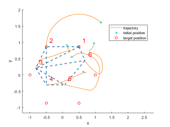
(b) Agents fail to converge to the correct formation.

(c) A good sensing graph.

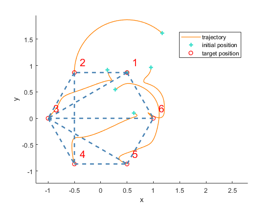
(d) Agents do converge to the correct formation.

Figure 1: Example demonstrating the challenge of formation control with directed sensing.

The most significant result in the study of bearing-only formation control over directed sensing was presented in [18]. In this work, they showed that for a special class of directed graphs, known as the leader first follower (LFF) graphs, the bearing-only formation control law proposed in [7] but adapted for directed sensing almost globally converges to the desired formation. The main idea of this work is that these LFF graphs lead to a cascade system structure facilitating the stability and convergence proof. Nevertheless, LFF graphs are restrictive and this work aims to extend the class of directed graphs that can be used to solve the bearing formation control problem with directed sensing.

The contribution of this paper focuses on extending the LFF structure to solve the bearing-only formation control problem over directed graphs. In this direction, our first result considers a simpler setup consisting of a single follower agent and many leaders. We provide an analysis to characterize the equilibria configuration for this system and discuss their stability and convergence properties. It turns out that the analysis of this simpler system is crucial for a more general extension of LFF graphs, which leads to our second contribution. We extend the BOFC framework to accommodate augmented LFF graphs, incorporating additional forward-directed edges while preserving the cascade structure of the system. We provide an analysis of the corresponding equilbria and stability of the system. Lastly, we provide simulation studies to demonstrate the feasibility and performance improvements enabled by the proposed extensions, showcasing faster convergence rates and increased flexibility in network design. These results offer a significant step toward more robust and adaptable BOFC solutions in directed sensing scenarios.

The remainder of this paper is organized as follows. Section II provides a brief overview of bearing-only formation control (BOFC) and revisits key results for undirected and directed graphs. Section III presents our main contributions, beginning with an analysis of the one-to-many BOFC setup and extending to LFF graph structures with additional forawrd edges. Section IV illustrates the theoretical results with numerical simulations, highlighting performance improvements, and demonstrating the feasibility of the proposed methods. Finally, Section V concludes the paper and discusses potential directions for future work.

Notations

Throughout this paper, $\mathbb{R}^{n}$ denotes the $n$-dimensional real vector space, and $\|\cdot\|$ represents the Euclidean norm for vectors. The identity matrix of size $n\times n$ is denoted by ${I}_{n}$, while $\vmathbb{1}_{n}$ represents the all-ones vector of dimension $n$. For a set of matrices or vectors $\{A_{i}\}_{i=1}^{n}$, $\mathrm{diag}(A_{i})_{i=1}^{n}$ denotes the block diagonal matrix with $A_{i}$ as its diagonal blocks. When the set of matrices are clear from context we write only $\mathrm{diag}(A_{i})$. The Kronecker product is denoted by $\otimes$. The image and kernel of a matrix $A$ are represented by $\operatorname{\mathrm{IM}}(A)$ and $\operatorname{\mathrm{Ker}}(A)$, respectively.

II Bearing-Only Formation Control

In this section we provide a brief overview of bearing only formation control (BOFC) problem for the both undirected and directed settings. We begin with the general setup and then present the key results from [7] and [18].

We consider a network of $n$ agents described by the integrator dynamics,

$$\dot{p}_{i}(t) =u_{i}(t),\;i=1,\ldots,n,$$ (1)

where $p_{i}(t),u_{i}(t)\in\mathbb{R}^{\mathrm{d}}$ are, respectively, the position and velocity control of each agent. Here, $\mathrm{d}$ represents the ambient dimension for the system, and we typically assume $\mathrm{d}\in\{2,3\}$. The vector $p(t)=\begin{bmatrix}p_{1}(t)^{T}&\cdots&p_{n}(t)^{T}\end{bmatrix}^{T}$ is denoted as the system configuration.

Agents can interact with each other according to a static graph, described by the pair $\mathcal{G}=(\mathcal{V},\mathcal{E})$. Here $\mathcal{V}=\{1,\ldots,n\}$ is the node set, and $\mathcal{E}\subseteq\mathcal{V}\times\mathcal{V}$ is the edge set. The notation $ij\in\mathcal{E}$ denotes that node $i\in\mathcal{V}$ is connected to node $j\in\mathcal{V}$. The graph may be undirected, in which case if $ij\in\mathcal{E}$, then $ji\in\mathcal{E}$, or directed which means that $ij\in\mathcal{E}$ does not imply that $ji\in\mathcal{E}$ [19].

A bearing formation is the vector $\bm{\mathrm{g}}=\begin{bmatrix}\bm{\mathrm{g}}_{1}^{T}&\cdots&\bm{\mathrm{g}}_{|\mathcal{E}|}\end{bmatrix}\in\mathbb{R}^{\mathrm{d}|\mathcal{E}|}$ specifying the desired bearing between neighboring agents. Naturally, we are concerned with bearing formations that are actually realizable by some configuration $\mathrm{p}\in\mathbb{R}^{\mathrm{d}n}$. In this direction, we introduce the notion of the bearing function, $F_{B}:\mathbb{R}^{\mathrm{d}n}\to\mathbb{R}^{\mathrm{d}|\mathcal{E}|}$, defined as

$$F_{B}(p) =\begin{bmatrix}g_{1}^{T}&\cdots&g_{|\mathcal{E}|}^{T}\end{bmatrix}^{T},$$ (2)

where for edge $k=ij\in\mathcal{E}$, the vector $g_{k}$ is the unit vector pointing from $p_{i}$ to $p_{j}$,

$$g_{k}:=g_{ij}=\frac{p_{j}-p_{i}}{\|p_{j}-p_{i}\|}.$$ (3)

With this notation, we define a bearing formation, $(\mathcal{G},g)$, by associating the edges in the graph $\mathcal{G}$ with the bearing measurements $g=F_{B}(p)$. We now provide a formal definition for a realizable bearing formation.

Definition 1.

A bearing formation $(\mathcal{G},\mathrm{g})$ is realizable in $\mathbb{R}^{\mathrm{d}}$ if there exists a configuration $\mathrm{p}\in\mathbb{R}^{\mathrm{d}n}$ satisfying $\mathrm{p}\in F_{B}^{-1}(\mathrm{g})$.

We now present the general bearing-only formation control problem. Note that the above set-up and the following problem statement does not depend on whether $\mathcal{G}$ is directed or undirected. In the sequel we will explore how directedness affects the solutions.

Problem 1.

Consider a collection of $n$ agents described by (1) that interact over a graph $\mathcal{G}$ and let $(\mathcal{G},\bm{\mathrm{g}})$ be a realizable bearing formation. Design a distributed control for each agent using only bearing measurements obtained from neighboring agents, i.e., a control of the form $u_{i}(t)=\sum_{ij\in\mathcal{E}}\kappa_{ij}(g_{ij},\bm{\mathrm{g}}_{ij})$ that drives the system to the target formation, i.e.,

$$\lim_{t\to\infty}g(t)=\lim_{t\to\infty}F_{B}(p(t))=\bm{\mathrm{g}}.$$

We now review the solutions to Problem 1 for the undirected and directed cases.

II-A BOFC for Undirected Graphs

A solution to Problem 1 for undirected graphs was initially proposed in [7]. The control strategy has the form

$$u_{i}(t) =-\sum_{ij\in\mathcal{E}}P_{g_{ij}(t)}\bm{\mathrm{g}}_{ij},\,i=1,\ldots,n,$$ (4)

where $P_{x}\in\mathbb{R}^{\mathrm{d}\times\mathrm{d}}$ is the orthogonal projection matrix defined as

$$P_{x}=I_{\mathrm{d}}-\frac{x}{\|x\|}\frac{x^{T}}{\|x\|}.$$ (5)

It is convenient to represent the control (4) in an aggregated matrix form as

$$u(t)=\bar{H}^{T}\operatorname{\mathrm{diag}}(P_{g_{ij}(t)})\bm{\mathrm{g},}$$ (6)

where $\bar{H}\in\mathbb{R}^{{\mathrm{d}}|\mathcal{E}|\times{\mathrm{d}}n}$ is the incidence matrix associated with the graph $\mathcal{G}$, defined as

$$[\bar{H}]_{ki}=\begin{cases}I_{\mathrm{d}},&\text{node }i\text{ is positive end of edge }e_{k}\\ -I_{\mathrm{d}},&\text{node }i\text{ is negative end of edge }e_{k}\\ 0,&\text{otherwise}.\end{cases}$$ (7)

The matrix form of the control (6) turns out to be related to the bearing rigidity matrix for a bearing framework. The bearing rigidity matrix is defined by the Jacobian of the bearing function $F_{B}$, and has the form

$$R_{B}(p)=\operatorname{\mathrm{diag}}\left(\frac{P_{g_{ij}}}{d_{ij}}\right)\bar{H},$$

where $d_{k}=d_{ij}=\|p_{i}-p_{j}\|$ is the distance between points $p_{i}$ and $p_{j}$ when $ij\in\mathcal{E}$. With this definition, the control can be expressed as

$$u(t)=\operatorname{\mathrm{diag}}(d_{ij})R_{B}(p)^{T}\bm{\mathrm{g}}.$$

For details on bearing rigidity theory and the bearing rigidity matrix, the reader is referred to [7]. The main result from [7] states that if the target bearing formation is infinitesimally bearing rigid, then the control (6) almost globally and exponentially converges to the desired formation.

II-B BOFC for Directed Graphs

A natural approach for solving Problem 1 for directed graphs is to simply try the same control as in (4), where the sum over the edges $ij\in\mathcal{E}$ are now directed. The aggregated matrix version of the control takes a slightly modified form arising from a redefinition of the incidence matrix for directed graphs. Define now the out-incidence matrix for the directed graph $\mathcal{G}$, denoted as $\bar{H}_{\otimes}\in\mathbb{R}^{\mathrm{d}|\mathcal{E}|\times\mathrm{d}n}$, as

$$[\bar{H}_{\otimes}]_{ki}=\begin{cases}I_{\mathrm{d}},&\text{node }i\text{ is positive end of edge }e_{k}\\ 0,&\text{otherwise}.\end{cases}.$$ (8)

Then the proposed control takes the form

$$u(t)=\bar{H}_{\otimes}^{T}\operatorname{\mathrm{diag}}(P_{g_{ij}(t)})\bm{\mathrm{g}}.$$ (9)

We now recall the example shown in Figure 1. In this example, the undirected version of the graph leads to a target bearing formation that is minimally infinitesimally bearing rigid, and therefore the undirected control (6) solves Problem 1. However, the example shows that depending on what orientation is used to solve the problem over directed graphs, it may or may not converge to the correct formation. One of the main contributions of [18] was to propose a class of directed graphs that solve Problem 1 using the control (9).

Definition 2.

A directed graph is a leader-first follower (LFF) graph if

• there is a vertex with no outgoing edges, denoted as the leader, assigned the label $v_{1}$;

• there is a vertex with only one outgoing edge pointing to the leader, denoted as the first follower assigned the label $v_{2}$;

• every vertex other than the leader and first follower has exactly two outgoing edges;

• for every directed edge $e_{ij}$, the label is ordered as $i>j$.

An example of an LFF graph is shown in Figure 2. Here, the leader is identified by the red node and the first follower by the dark blue node. We denote any edge $e_{ij}$ with $i>j$ as a forward edge. With this notion we see LFF graphs consist only of forward edges.

Figure 2: An example of an LFF graph.

Of note for the BOFC on these LFF graphs is the resulting cascade structure of the closed-loop system. Indeed, for LFF graphs, the dynamics become

$$\begin{cases}\dot{p}_{1}(t)&=0\\ \dot{p}_{2}(t)&=p_{1}(t)-d_{21}(t)\bm{\mathrm{g}}_{21}\\ \dot{p}_{i}(t)&=-\sum_{ij\in\mathcal{E}}P_{g_{ij}(t)}\bm{\mathrm{g}}_{ij},\,i=3,\ldots,n\end{cases}.$$

The main result then from [18] states that if the target formation is an LFF graph, the control (9) solves Problem 1. The proof relies on the stability of cascade systems and the fact that the leader and first follower effectively fix the centroid and scale of the formation.

III Extending the LFF Structure

Extending the class of directed graphs that can solve Problem 1 poses significant challenges. The moment the LFF structure is broken, then the cascade system analysis from [18] may no longer be applied. Nevertheless, there is an interest to find additional structures that can be used, enabling a network designer to have more flexibility to design systems with additional properties such as performance or robustness. To emphasize this point, we refer again to the example of Figure 1(c) which solves Problem 1 but is not an LFF graph indicating that such structures exist.

To begin, we focus on a simple system comprised of one follower and many leaders. This is not an LFF graph, and the analysis of this simpler problem will provide the framework needed to extend the LFF graphs.

III-A BOFC with 1 Follower and Many Leaders (1-to-many)

We consider $n\geq 3$ agents modeled by the dynamics (1) with $n-1$ leaders and one follower. We denote the leaders by the first $n-1$ nodes, and thus the follower is node $n$. The directed graph has edges only of the form $ni\in\mathcal{E}$ for $i=1,\ldots,n-1$. An example of this structure is shown in Figure 3.

Figure 3: The directed graph for the 1-to-many setup.

With this setup, and applying the control (4), the dynamics of each agent can be expressed as

$$\dot{p}_{i}(t) =0,\,i=1,\ldots,n-1$$ (10)

$$\dot{p}_{n}(t) =-\sum_{nj\in\mathcal{E}}P_{g_{nj}(t)}\bm{\mathrm{g}}_{nj}.$$

We now introduce an assumption of the target formation for this setup.

Assumption 1.

The target bearing formation $(\mathcal{G},\bm{\mathrm{g}})$ is realizable. Furthermore, there exists a configuration $\mathrm{p}\in F_{B}^{-1}(\bm{\mathrm{g}})$ such that $\mathrm{p}_{i},\mathrm{p}_{j}$ and $\mathrm{p}_{n}$ are not collinear for any $i,j\in\{1,2,\ldots,n-1\}$.

Moreover, according to (10), the leader nodes do not move. Thus, the realizability question can be framed in terms of the initial conditions of the leader agents. That is, for a configuration $\mathrm{p}$ satisfying Assumption 1, we must have that $p_{i}(0)=\mathrm{p}_{i}$ for $i=1,\ldots,n-1$. We are now prepared to present the first result which characterizes the equilibrium configuration of (10).

To begin, we note that the solution to the equilibrium condition

$$0=\kappa(g,\bm{\mathrm{g}})=\sum_{ij\in\mathcal{E}}\kappa_{ij}(g_{ij},\bm{\mathrm{g}}_{ij})=-\sum_{nj\in\mathcal{E}}P_{g_{nj}(t)}\bm{\mathrm{g}}_{nj}$$

can be expressed more naturally in terms of the bearings $\mathrm{g}_{nj}$. Let the set $\mathcal{X}(\mathcal{G},\bm{\mathrm{g}})$ be the set of bearings satisfying the equilibrium condition. This set has a special structure, so we express it as the intersection of three sets,

$$\mathcal{X}(\mathcal{G},\bm{\mathrm{g}}) =\mathcal{X}_{eq}(\mathcal{G},\bm{\mathrm{g}})\cap\mathcal{C}_{1}\cap\mathcal{C}_{F_{B}}(\mathcal{G}).$$ (11)

The first set, $\mathcal{X}_{eq}(\mathcal{G},\bm{\mathrm{g}})$, characterizes all vectors that satisfy the equilibrium condition, i.e.,

$$\mathcal{X}(\mathcal{G},\bm{\mathrm{g}})=\{x\in\mathbb{R}^{\mathrm{d}|\mathcal{E}|}:\kappa(x,\bm{\mathrm{g}})=0\}.$$ (12)

Note that this set may include solutions that are not bearing vectors (i.e., not unit-norm vectors). The set

$${\scriptsize{\mathcal{C}_{1}=\{g={\tiny{\begin{bmatrix}g_{1}^{T}&\hskip-3.0pt\cdots\hskip-3.0pt&g^{T}_{|\mathcal{E}|}\end{bmatrix}^{T}}}\in\mathbb{R}^{\mathrm{d}|\mathcal{E}|}:\|g_{k}\|=1,\,k=1,\ldots,|\mathcal{E}|\}\}}}$$ (13)

ensures all $\mathrm{d}$-vector entries of $\mathrm{g}$ are unit-norm vectors. Finally, the set

$$\mathcal{C}_{F_{B}}(\mathcal{G})=\{g\in\mathbb{R}^{\mathrm{d}|\mathcal{E}|}\,:\,\exists\,p\in\mathbb{R}^{d|\mathcal{V}|}\text{ s.t. }g=F_{B}(p)\},$$ (14)

considers only bearings that are realizable. In fact, it is true that $\mathcal{C}_{F_{B}(\mathcal{G})}\subset\mathcal{C}_{1}$, but our analysis is aided by examining these sets separately.

Of interest now is to understand what vectors lie in the set $\mathcal{X}(\mathcal{G},\bm{\mathrm{g}})$. We note that the equilibrium condition is nonlinear in the bearing $\mathrm{g}$, but is linear in the target bearing $\bm{\mathrm{g}}$. In this direction, we may ask given a set of measured bearings $\mathrm{g}$, what are all possible target formations that result in an equilibrium? This can also be characterized by the intersection of three sets,

$$\mathcal{Y}(\mathcal{G},g) =\mathcal{Y}_{eq}(\mathcal{G},g)\cap\mathcal{C}_{1}\cap\mathcal{C}_{F_{B}}(\mathcal{G}),$$ (15)

where

$$\mathcal{Y}_{eq}(\mathcal{G},g) =\{y\in\mathbb{R}^{\mathrm{d}|\mathcal{E}|}:\kappa(g,y)=0\}.$$ (16)

We now describe how the sets $\mathcal{X}(\mathcal{G},\bm{\mathrm{g}})$ and $\mathcal{Y}(\mathcal{G},{g})$ are related.

Lemma 1.

Assume that $g,\bm{\mathrm{g}}\in\mathcal{C}_{1}\bigcap\mathcal{C}_{F_{B}}(\mathcal{G})$. Then

• $\bm{\mathrm{g}}\in\mathcal{X}(\mathcal{G},\bm{\mathrm{g}})$, and

• $g\in\mathcal{Y}(\mathcal{G},g)$.

Proof.

By assumption, both formations $(\mathcal{G},g)$ and $(\mathcal{G},\bm{\mathrm{g}})$ are realizable bearing formations. From the properties of the projection matrices, it follows that $P_{g_{k}}g_{k}=0$ and $P_{\bm{\mathrm{g}_{k}}}\bm{\mathrm{g}_{k}}=0$ for $k=1,\ldots,|\mathcal{E}|$, and therefore $\bm{\mathrm{g}}\in\mathcal{X}_{eq}(\mathcal{G},\bm{\mathrm{g}})$ and ${g}\in\mathcal{Y}_{eq}(\mathcal{G},{g})$. ∎

Lemma 1 shows that the sets $\mathcal{X}(\mathcal{G},\bm{\mathrm{g}})$ and $\mathcal{Y}(\mathcal{G},g)$ are always non-empty. We would further like to understand under what conditions does the set $\mathcal{X}(\mathcal{G},\bm{\mathrm{g}})$ only contain the target formation, i.e., that there is a single equilibrium for the dynamics (10).

Lemma 2.

For the system (10), if $\mathcal{Y}(\mathcal{G},{\bar{\mathrm{g}}})=\{{\bar{\mathrm{g}}}\}$ for some bearing vector ${\bar{\mathrm{g}}}\in\mathcal{C}_{1}\cap\mathcal{C}_{F_{B}}(\mathcal{G})$, then $\mathcal{X}(\mathcal{G},\bm{\mathrm{g}})=\{\bm{\mathrm{g}}\}$ for target bearing vector $\bm{\mathrm{g}}\in\mathcal{C}_{1}\cap\mathcal{C}_{F_{B}}(\mathcal{G})$.

Proof.

The lemma is proven by contradiction. Assume that $\mathcal{X}(\mathcal{G},\bm{\mathrm{g})})=\{\bm{\mathrm{g}},{\bar{\mathrm{g}}}\}$, which means that $\kappa(\bm{\mathrm{g}},\bm{\mathrm{g}})=\kappa({\bar{\mathrm{g}}},\bm{\mathrm{g}})=0$. This then implies that $\bm{\mathrm{g}}\in\mathcal{Y}(\mathcal{G},{\bar{\mathrm{g}}})$ and from Lemma 2 we have $\{\bm{\mathrm{g}},{\bar{\mathrm{g}}}\}\subseteq\mathcal{Y}(\mathcal{G},{\bar{\mathrm{g}}})$, leading to a contradiction. ∎

Lemmas 1 and 2 show that if $\mathcal{Y}(\mathcal{G},g)$ is a singleton, than so must be $\mathcal{X}(\mathcal{G},\bm{\mathrm{g})})$. We now derive conditions that guarantee that this in fact happens. We achieve this by providing an explicit characterization of the sets $\mathcal{Y}_{eq}(\mathcal{G},g)$, $\mathcal{Y}_{eq}(\mathcal{G},g)\cap\mathcal{C}_{1}$, and finally $\mathcal{Y}(\mathcal{G},g)$.

We start by finding the elements in $\mathcal{Y}_{eq}(\mathcal{G},g)$. Define $\tilde{P}$ as

$$\tilde{P}=\begin{bmatrix}P_{g_{n1}}&\cdots&P_{g_{n(n-1)}}\end{bmatrix}\in\mathbb{R}^{\mathrm{d}\times\mathrm{d}(n-1)}.$$

Then, the equilibrium condition for the follower node $n$ in (10) can be expressed as

$$0=-\sum_{nj\in\mathcal{E}}P_{g_{nj}}{\bm{\mathrm{g}}_{nj}}=\tilde{P}{\bm{\mathrm{g}}}.$$ (17)

It then follows that $\mathcal{Y}_{eq}(\mathcal{G},g)=\operatorname{\mathrm{Ker}}(\tilde{P})$. For formations in $\mathbb{R}^{\mathrm{d}n}$, it follows that $\mathrm{rk}\tilde{P}=\mathrm{d}$, and the dimension of its null-space is therefore $\mathrm{d}(n-2)$.

Let $G=\mathrm{diag}\{g_{ni}\}_{i=1}^{n-1}\in\mathbb{R}^{\mathrm{d}(n-1)\times n-1}$ and $G^{\perp}=\mathrm{diag}\{g_{ni}^{\perp}\}_{i=1}^{n-1}\in\mathbb{R}^{\mathrm{d}(n-1)\times(\mathrm{d}-1)(n-1)}$, where $g_{ni}^{\perp}\in\mathbb{R}^{\mathrm{d}\times\mathrm{d}-1}$ is defined such that $\operatorname{\mathrm{IM}}(g_{ni}^{\perp})=\operatorname{\mathrm{Ker}}(g_{ni}^{T})$. It then follows that $\operatorname{\mathrm{IM}}(G)$ and $\operatorname{\mathrm{IM}}(G^{\perp})$ are orthogonal subspaces, and that $\operatorname{\mathrm{IM}}(G)\oplus\operatorname{\mathrm{IM}}(G^{\perp})=\mathbb{R}^{\mathrm{d}(n-1)}$.

The following lemma relates properties of $G$ and $G^{\perp}$ to the matrix $\tilde{P}$.

Lemma 3.

For $G$ and $G^{\perp}$ defined above, the following hold:

• $\tilde{P}G=\vmathbb{0}_{\mathrm{d}\times n-1}$;

• $\tilde{P}G^{\perp}=\begin{bmatrix}g_{n1}^{\perp}&\cdots&g_{n(n-1)}^{\perp}\end{bmatrix}\in\mathbb{R}^{\mathrm{d}\times(\mathrm{d}-1)(n-1)}$.

Proof.

The proof follows by direct construction. For part $i$), we have

$$\tilde{P}G =\begin{bmatrix}P_{g_{n1}}g_{n1}&\cdots&P_{g_{n(n-1)}}g_{n(n-1)}\end{bmatrix}=\vmathbb{0}_{\mathrm{d}\times n-1}.$$

Similarly, for $ii$) we have $P_{g_{ni}}\mathrm{g}_{ni}^{\perp}=\mathrm{g}_{ni}^{\perp}$ and the result follows directly. ∎

Lemma 3 shows that $\operatorname{\mathrm{IM}}(G)\subset\operatorname{\mathrm{Ker}}(\tilde{P})$. The columns of $G$ therefore can be used to determine $n-1$ basis vectors of $\operatorname{\mathrm{Ker}}(\tilde{P})$, while there are $m=\mathrm{d}(n-2)-n+1$ basis vectors left to be determined. These basis vectors should be orthogonal to $G$, which can be expressed by the linear combination of the columns of $G^{\perp}$.

In this direction, define $N\in\mathbb{R}^{(\mathrm{d}-1)(n-1)\times m}$ such that $\operatorname{\mathrm{IM}}(N)=\operatorname{\mathrm{Ker}}(\tilde{P}G^{\perp})$, i.e., $\tilde{P}G^{\perp}N=\vmathbb{0}_{\mathrm{d}\times m}$, from which it follows that $\operatorname{\mathrm{IM}}(G^{\perp}N)\subset\operatorname{\mathrm{Ker}}(\tilde{P})$. Thus, we conclude that

$$\operatorname{\mathrm{Ker}}(\tilde{P})=\operatorname{\mathrm{IM}}(G)\oplus\operatorname{\mathrm{IM}}(G^{\perp}N).$$

We are now prepared to express $\mathcal{Y}_{eq}(\mathcal{G},g)$ in terms of linear combinations of the columns of $G$ and $G^{\perp}N$,

$$\mathcal{Y}_{eq}(\mathcal{G},g)=\{y\in\mathbb{R}^{\mathrm{d}|\mathcal{E}|}:y=Ga+G^{\perp}Nb,\,\forall\,a\in\mathbb{R}^{n-1},\,b\in\mathbb{R}^{m}\}.$$

Equivalently, we can express vectors $y\in\mathcal{Y}_{eq}(\mathcal{G},g)$ in terms of its components as

$$y_{i}=a_{i}g_{ni}+g_{ni}^{\perp}\left(\sum_{j=1}^{m}b_{j}n_{ij}\right),$$ (18)

where $n_{ij}\in\mathbb{R}^{\mathrm{d}-1}$ and

$$N=\begin{bmatrix}n_{11}&\cdots&n_{1m}\\ \vdots&\ddots&\vdots\\ n_{(n-1)1}&\cdots&n_{(n-1)m}\end{bmatrix}.$$

We now use the characterization in (18) to find all solutions that are also in $\mathcal{C}_{1}$. In particular, we must have that for each $i$,

$$\|y_{i}\|^{2} =\left(a_{i}g_{ni}+g_{ni}^{\perp}\left(\sum_{j=1}^{m}b_{j}n_{ij}\right)\right)^{T}\left(a_{i}g_{ni}+g_{ni}^{\perp}\left(\sum_{j=1}^{m}b_{j}n_{ij}\right)\right)$$

$$=a_{i}^{2}+\left\|\sum_{j=1}^{m}b_{j}n_{ij}\right\|^{2}=1.$$

This holds since $g_{ni}^{T}g_{ni}^{\perp}=0$ and $(g_{ni}^{\perp})^{T}g_{ni}^{\perp}=I_{\mathrm{d}-1}$.

Finally, we can consider the realizable vectors described by the form above.

Lemma 4.

In the 1-to-many system, the bearing vector $\mathrm{g}\in\mathcal{Y}_{eq}(\mathcal{G},g)\cap\mathcal{C}_{1}$ is realizable if and only if $a=\vmathbb{1}_{n-1},\,b=\vmathbb{0}_{m}$. Equivalently, $\mathcal{Y}(\mathcal{G},g)=\{g\}$.

Proof.

($\Leftarrow$) For $a=\vmathbb{1}_{n-1},\,b=\vmathbb{0}_{m}$ we have $g=Ga+G^{\perp}Nb=g$. The vector $g$ corresponds to a bearing measurement, it must be realizable.

($\Rightarrow$) We prove this by contradiction. Assume there exists an $a\neq\vmathbb{1}_{n-1}$ and $b\neq\vmathbb{0}_{m}$ such that the bearing vector $\bar{g}=Ga+G^{\perp}Nb\in\mathcal{C}_{1}\cap\mathcal{C}_{F_{B}}$. Therefore, we have that $\{\bar{g},g\}\subseteq\mathcal{Y}(\mathcal{G},g)$. Let $\bar{p}$ and $p$ be such that $\bar{g}=F_{B}(\bar{p})$ and ${g}=F_{B}(p)$.

Since the leader positions are fixed, we can consider the displacement between the follower agent of the two solutions described above. Therefore, let $z=\bar{p}_{n}-p_{n}$, and for each $i=1,\ldots,n-1$,

$$z_{i} =\bar{p}_{n}-p_{i}+p_{i}-p_{n}$$ (19)

$$=\bar{d}_{ni}\bar{g}_{ni}-d_{ni}{g}_{ni}$$

$$=(\bar{d}_{ni}a_{i}-d_{ni})g_{ni}+g_{ni}^{\perp}\left(\sum_{j=1}^{m}b_{j}n_{ij}\bar{d}_{ni}\right),$$

where $d_{ni}=\|p_{n}-p_{i}\|$ and $\bar{d}_{{n}i}=\|\bar{p}_{n}-p_{i}\|$.

Multiplying on the left by $z_{i}^{T}$ of $g_{ni}^{\perp}\left(\sum_{j=1}^{m}b_{j}n_{ij}\right)$ gives

$$z_{i}^{T}g_{ni}^{\perp}\left(\sum_{j=1}^{m}b_{j}n_{ij}\right)$$ (20)

$$= \left((\bar{d}_{ni}a_{i}-d_{{n}i})g_{ni}^{T}+\bar{d}_{ni}\left(\sum_{j=1}^{m}b_{j}n_{ij}\right)^{T}(g_{ni}^{\perp})^{T}\right)g_{ni}^{\perp}\left(\sum_{j=1}^{m}b_{j}n_{ij}\right)$$

$$=\bar{d}_{ni}\left(\sum_{j=1}^{m}b_{j}n_{ij}\right)^{T}\left(\sum_{j=1}^{m}b_{j}n_{ij}\right)\geq 0.$$

On the other hand, the following equation always holds,

$$(\vmathbb{1}_{n}^{T}\otimes I_{\mathrm{d}})G^{\perp}Nb=\vmathbb{0}_{\mathrm{d}}\Leftrightarrow\sum_{i=1}^{n-1}\left(g_{ni}^{\perp}\sum_{j=1}^{m}b_{j}n_{ij}\right) =\vmathbb{0}_{\mathrm{d}},$$ (21)

since $(\vmathbb{1}_{n}^{T}\otimes I_{\mathrm{d}})G^{\perp}=\tilde{P}G^{\perp}=[g_{n1}^{\perp},\cdots,g_{n(n-1)}^{\perp}]$. Any vector multiplied by zero is zero, which leads to

$$z_{i}^{T}\sum_{i=1}^{n-1}\left(g_{ni}^{\perp}\sum_{j=1}^{m}b_{j}n_{ij}\right)=\sum_{i=1}^{n-1}\left(z_{i}^{T}g_{ni}^{\perp}\sum_{j=1}^{m}b_{j}n_{ij}\right) =0.$$ (22)

From (20) and (22), it can concluded that $z_{i}^{T}g_{ni}^{\perp}\sum_{j=1}^{m}b_{j}n_{ij}\geq 0$ for all terms with $i=1,\cdots,n-1$ and their sum equals to zero. Thus, every single term should be exactly zero, which means $(\bar{d}_{ni}a_{i}-d_{{n}i})g_{ni}+g_{ni}^{\perp}\left(\sum_{j=1}^{m}b_{j}n_{ij}\bar{d}_{ni}\right)=0$. This equation then directly leads to $a_{i}=1,\forall i=1,\ldots,n-1$ and $b_{j}=0,\forall j=1,\ldots,m$. ∎

Lemma 4 shows that $\mathcal{Y}(\mathcal{G},g)=\{g\}$. It then follows from Lemma 2 that $\mathcal{X}(\mathcal{G},\bm{\mathrm{g}})=\{\bm{\mathrm{g}}\}$. We now show that the equilibrium position of the follower agent, $\mathrm{p}_{n}$ can be uniquely determined from the initial conditions (target positions) of the leaders and the bearing measurements.

Proposition 1.

Let Assumption 1 hold for the target bearing formation $(\mathcal{G},\bm{\mathrm{g}})$ and assume that $p_{i}(0)=\mathrm{p}_{i}$ for a configuration $\mathrm{p}\in F_{B}^{-1}(\bm{\mathrm{g}})$. Then

$$\mathrm{p}_{n}=\left(\sum_{nj\in\mathcal{E}}P_{\bm{\mathrm{g}}_{nj}}\right)^{-1}\left(\sum_{nj\in\mathcal{E}}P_{\bm{\mathrm{g}}_{nj}}\mathrm{p}_{j}\right)$$ (23)

is an equilibrium of (10).

Proposition 1 translates the equilibrium from conditions on the bearing measurements to the position of agent $n$. Before proving it, we present a useful lemma related to the properties of the projection matrix.

Lemma 5.

Let $x,y\in\mathbb{R}^{\mathrm{d}}$ be two non-parallel vectors. Then $P_{x}+P_{y}$ is invertible.

Proof.

From the definition of the projection matrix (5), it follows that $\operatorname{\mathrm{Ker}}(P_{x})=\operatorname{\mathrm{span}}\{x\}$ and $\operatorname{\mathrm{Ker}}(P_{y})=\operatorname{\mathrm{span}}\{y\}$. Since $x$ is not parallel with $y$, the subspace

$$\operatorname{\mathrm{Ker}}(P_{x})\cap\operatorname{\mathrm{Ker}}(P_{y})=\operatorname{\mathrm{span}}\{x\}\cap\operatorname{\mathrm{span}}\{y\}=\{0\}.$$

In addition, the projection matrix is positive semi-definite. The kernel of two positive semi-definite matrices is the intersection of the kernel space of these two matrices (i.e., $\operatorname{\mathrm{Ker}}(P_{x}+P_{y})=\operatorname{\mathrm{Ker}}(P_{x})\bigcap\operatorname{\mathrm{Ker}}(P_{y})$). Thus, the space $\operatorname{\mathrm{Ker}}(P_{x}+P_{y})=\{0\}$, implying that $P_{x}+P_{y}$ is invertible. ∎

Proof of Proposition 1.

For the configuration $\mathrm{p}$, if $F_{B}(\mathrm{p})=\bm{\mathrm{g}}$, it always holds that

$$P_{\bm{\mathrm{g}_{nj}}}(\mathrm{p}_{n}-\mathrm{p}_{j})=0,\forall nj\in\mathcal{E}.$$

Furthermore, the sum

$$\sum_{nj\in\mathcal{E}}P_{\bm{\mathrm{g}_{nj}}}(\mathrm{p}_{n}-\mathrm{p}_{j})=0$$

must also hold. Rearranging terms leads to

$$\left(\sum_{nj\in\mathcal{E}}P_{\bm{\mathrm{g}_{nj}}}\right)\mathrm{p}_{n}=\sum_{nj\in\mathcal{E}}P_{\bm{\mathrm{g}_{nj}}}\mathrm{p}_{j}.$$

Assumption 1 requires $\bm{\mathrm{g}}_{ni}\neq\bm{\mathrm{g}}_{nj}\ \forall i,j=1,\ldots,n-1$, and it follows from Lemma 5 that $\left(\sum_{nj\in\mathcal{E}}P_{\bm{\mathrm{g}_{nj}}}\right)$ is invertible. As a result, the target position $\mathrm{p}_{n}$ in (23) holds. ∎

The last step is to determine the stability of equilibrium.

Theorem 1.

Let Assumption 1 hold for some target bearing configuration $(\mathcal{G},\bm{\mathrm{g}})$ and assume that $p_{i}(0)=\mathrm{p}_{i}$ for a $\mathrm{p}\in F_{B}^{-1}(\bm{\mathrm{g}})$. Then the point $\mathrm{p}_{n}$ defined in (23) is a globally exponentially stable equilibrium for the dynamics in (10).

Proof.

Consider the Lyapunov function $V(p_{n}(t))=\frac{1}{2}\|p_{n}(t)-\mathrm{p}_{n}\|^{2}$. Then

$$\dot{V}(p_{n}(t)) =(p_{n}(t)-\mathrm{p}_{n})^{T}\dot{p}_{n}(t)$$

$$\hskip-28.45274pt=-(p_{n}(t)-\mathrm{p}_{n})^{T}\sum_{nj\in\mathcal{E}}P_{g_{nj}(t)}\mathbf{g}_{nj}$$

$$\hskip-28.45274pt=-(p_{n}(t)-\mathrm{p}_{n})^{T}\sum_{nj\in\mathcal{E}}\frac{P_{g_{nj}(t)}}{d_{nj}(t)}(p_{j}(t)-\mathrm{p}_{n})$$

$$\hskip-28.45274pt=-(p_{n}(t)-\mathrm{p}_{n})^{T}\sum_{nj\in\mathcal{E}}\frac{P_{g_{nj}(t)}}{d_{nj}(t)}(p_{j}(t)-p_{n}(t)+p_{n}(t)-\mathrm{p}_{n})$$

$$\hskip-28.45274pt=-(p_{n}(t)-\mathrm{p}_{n})^{T}\left(\sum_{nj\in\mathcal{E}}\frac{P_{g_{nj}(t)}}{d_{nj}(t)}(p_{n}(t)-\mathrm{p}_{n})\right)$$

$$\hskip-28.45274pt=-(p_{n}(t)-\mathrm{p}_{n})^{T}\underbrace{\left(\sum_{nj\in\mathcal{E}}\frac{P_{g_{nj}(t)}}{d_{nj}(t)}\right)}_{M(t)}(p_{n}(t)-\mathrm{p}_{n}).$$ (24)

The projection matrices $P_{g_{ni}}(t)$ are positive semi-definite. Thus, the matrix $M(t)=\sum_{nj\in\mathcal{E}}\frac{P_{g_{nj(t)}}}{d_{nj}(t)}\geq 0$, indicating $\dot{V}(p_{n}(t))\leq 0$ along the system trajectories. The equality holds ($\dot{V}=0$) if and only if $(p_{n}(t)-\mathrm{p}_{n})\in\operatorname{\mathrm{Ker}}(M(t))$, where the null space of $M(t)$ can be considered in two cases:

• If $p_{n}(t)$ is collinear with all the fixed agents, i.e., the bearing measurements $g_{n1},g_{n2},\cdots,g_{n(n-1)}$ are parallel and the projection matrices satisfy $P_{g_{n1}}=P_{g_{n2}}=\cdots=P_{g_{n(n-1)}}$, then the matrix $M(t)$ can be simplified as $M(t)=P_{g_{n1}(t)}\left(\sum_{nj\in\mathcal{E}}\frac{1}{d_{nj}(t)}\right)$ and $\operatorname{\mathrm{Ker}}(M(t))=\operatorname{\mathrm{span}}\{g_{n1}\}$. From Assumption 1, any two target bearings $\mathbf{g}_{ni},\mathbf{g}_{nj},$ are not parallel, implying that $\mathrm{p}_{n}$ is not collinear with any two other fixed agents. Thus, $(p_{n}(t)-\mathrm{p}_{n})$ is not parallel with the bearing measurement $g_{n1}$ and $(p_{n}(t)-\mathrm{p}_{n})\notin\operatorname{\mathrm{Ker}}(M(t))$.

• If $p_{n}(t)$ is not collinear with all the fixed agents, i.e., the bearing measurements $g_{ni}$ and $g_{nj}$ are not parallel for any $i,j$, then the sum of the projection matrices $P_{g_{ni}}+P_{g_{nj}}$ is invertible and positive definite (see Lemma 5). All the other terms of $M(t)$ are positive semi-definite, so $M(t)$ must be positive definite. In this case, $\dot{V}=0$ if and only if $p_{n}(t)-\mathrm{p}_{n}=0$.

As a result, $\dot{V}(p_{n}(t))\leq 0$ and equality holds only when $p_{n}(t)$ reaches the equilibrium $\mathrm{p}_{n}$. Thus $\mathrm{p}_{n}$ asymptotically stable.

We now show exponential stability. Since $M(t)$ is positive definite, we can define $\bar{\lambda}=\min_{t}\lambda_{min}(M(t))>0$. Therefore,

$$\dot{V}(p_{n}(t))\leq-(p_{n}(t)-\mathrm{p}_{n})^{T}{M(t)}(p_{n}(t)-\mathrm{p}_{n})\leq-\bar{\lambda}V(p_{n}(t)),$$

showing exponential stability. ∎

For the 1-to-many system with at least 2 leaders, the follower $p_{n}$ asymptotically converges to the target position specified in (23) exponentially fast. One can also see that as the number of leader nodes increases, the Lyapunov exponent $\bar{\lambda}$ also increases, a direct consequence of Weyl’s inequality [20].

We conclude this section by examining a special configuration of the 1-to-many system that admits only an unstable equilibrium. We consider initial conditions for the leaders that satisfy $p_{i}(0)=\bar{\mathrm{p}}_{i},\,i=1,\ldots,n-1$ for a $\bar{\mathrm{p}}\in F_{B}^{-1}(-\bm{\mathrm{g}})$. In this direction, we first introduce the notion of symmetric configurations.

Definition 3.

Two configurations $p=[p_{1}^{T}\ \cdots\ p_{n}^{T}]^{T}$ and $q=[q_{1}^{T}\ \cdots\ q_{n}^{T}]^{T}$ are symmetric with respect to $c$ if

$$p_{i}-c=c-q_{i},\;i=1,\ldots,n-1.$$

Proposition 2.

For the target formation $(\mathcal{G},\bm{\mathrm{g}})$, consider two configurations $\mathrm{p},\ \bar{\mathrm{p}}\in\mathbb{R}^{|\mathcal{V}|\mathrm{d}}$. If $\mathrm{p}$ and $\bar{\mathrm{p}}$ are symmetric with respect to some point $c\in\mathbb{R}^{\mathrm{d}}$, and $\mathrm{p}\in F_{B}^{-1}(\bm{\mathrm{g}})$, then $\bar{\mathrm{p}}\in F_{B}^{-1}(-\bm{\mathrm{g}})$.

Proof.

From Definition 3, it follows that

$$\mathrm{p}_{i}-c=c-\bar{\mathrm{p}}_{i},$$

or equivalently that $\bar{\mathrm{p}}_{i}=2c-\mathrm{p}_{i}$. Since $\mathrm{p}\in F_{B}^{-1}(\bm{\mathrm{g}})$, we also have that

$$\frac{\mathrm{p}_{i}-\mathrm{p}_{n}}{\|\mathrm{p}_{i}-\mathrm{p}_{n}\|}=\bm{\mathrm{g}}_{ni},\,i=1,\ldots,n-1.$$

Consider now the point $\bar{\mathrm{p}}_{n}$. Since $\mathrm{p}$ and $\bar{\mathrm{p}}$ are symmetric with respect to $c$, it follows that $\bar{\mathrm{p}}_{n}=2c-\mathrm{p}_{n}$. We then have

$$\frac{\bar{\mathrm{p}}_{i}-\bar{\mathrm{p}}_{n}}{\|\bar{\mathrm{p}}_{i}-\bar{\mathrm{p}}_{n}\|} =\frac{2c-\mathrm{p}_{i}-(2c-\mathrm{p}_{n})}{\|2c-\mathrm{p}_{i}-(2c-\mathrm{p}_{n})\|}$$

$$=-\frac{\mathrm{p}_{i}-\mathrm{p}_{n}}{\|\mathrm{p}_{i}-\mathrm{p}_{n}\|}=-\bm{\mathrm{g}_{ni}}.$$ (25)

Since equation (III-A) holds for every leader $i=1,\ldots,n-1$, it follows that $\bar{\mathrm{p}}\in F_{B}^{-1}(-\bm{\mathrm{g}})$ ∎

Lemma 6.

Let Assumption 1 hold for the target bearing formation $(\mathcal{G},\bm{\mathrm{g}})$ and assume that $p_{i}(0)=\bar{\mathrm{p}}_{i}$ for a configuration $\bar{\mathrm{p}}\in F_{B}^{-1}(-\bm{\mathrm{g}})$. Then

$$\mathrm{p}_{n}=\left(\sum_{nj\in\mathcal{E}}P_{\bm{\mathrm{g}}_{nj}}\right)^{-1}\left(\sum_{nj\in\mathcal{E}}P_{\bm{\mathrm{g}}_{nj}}\bar{\mathrm{p}}_{j}\right)$$

is the only equilibrium of (10) and it is unstable.

Proof.

First, recall that the control $\kappa(g,\bm{\mathrm{g}})$ is linear in the target bearing $\bm{\mathrm{g}}$. Therefore, it follows that $\kappa(g,\bm{\mathrm{g}})=-\kappa(g,-\bm{\mathrm{g}})$, and the BOFC for the bearing formation $(\mathcal{G},\bm{\mathrm{g}})$ has the same equilibrium point as the bearing formation $(\mathcal{G},-\bm{\mathrm{g}})$. Furthermore, the dynamics of the follower satisfies

$$\dot{p}_{n}(t)=\kappa(g,\bm{\mathrm{g}})=-\kappa(g,-\bm{\mathrm{g}})=\sum_{nj\in\mathcal{E}}P_{\mathrm{g}_{nj}(t)}(\bm{\mathrm{g}}_{nj}).$$

The equilibrium condition can now be verified using the same arguments as in Proposition 1. Using the same Lyapunov function construction as in Theorem 1 it is straightforward to verify that $\dot{V}(p_{n}(t))>0$. Applying Chetaev instability theorem we can conclude this equilbirum is unstable. ∎

A key point of this result shows that symmetric configurations for the leader initial conditions correspond to either stable or unstable trajectories. This result may not be suprising as we are choosing initial conditions for the leaders that do not correspond to desired bearing measurements. Nevertheless, this characterization will be important to establish equilibria and stability conditions for more general LFF graphs in the sequel.

III-B BOFC with Ordered LFF Graphs

In the previous section, we outlined an analysis approach for the one-to-many BOFC. This turns out to be a central idea when trying to generalize the LFF structures. In particular, we aim next to relax the assumption in Definition 2 that each follower agent must have exactly 2 outgoing edges. We call such graphs ordered LFF graphs. An example of an ordered LFF graph is showed in Figure 4, with the leader and first-follower as nodes $1,2$, respectively. Note that all edges are forward edges but it is possible for some nodes to have more than two outgoing edges.

Definition 4.

A directed graph is an ordered LFF graph (OLFF) if

• there is a vertex with no outgoing edges, denoted as the leader, assigned the label $v_{1}$;

• there is a vertex with only one outgoing edge pointing to the leader, denoted as the first follower assigned the label $v_{2}$;

• every vertex $v_{i}$ other than the leader and the first follower has at least two outgoing edges, pointing to vertices with indices smaller that $i$.

Figure 4: An example of an ordered LFF graph.

When considering the BOFC for directed graphs (9) over ordered LFF graphs, we reveal that it is still possible to express the dynamics in a cascade form. Indeed, for OLFF graphs, the dynamics for each agent can be expressed as

$$\begin{cases}\dot{p}_{1}(t)&=0\\ \dot{p}_{2}(t)&=p_{1}(t)-d_{21}(t)\bm{\mathrm{g}}_{21}\\ \dot{p}_{i}(t)&=-\sum_{ij\in\mathcal{E}}\kappa_{ij}(g_{ij},\bm{\mathrm{g}}_{ij}),\,i=3,\ldots,n\end{cases},$$ (26)

where we have that agent $i$ only requires information from agents with indices $j<i$.

Similar to Assumption 1, an assumption on the target bearing formation is required for Problem (1).

Assumption 2.

The target bearing formation $(\mathcal{G},\bm{\mathrm{g}})$ is realizable. Furthermore, there exists a configuration $\mathrm{p}\in F_{B}^{-1}(\bm{\mathrm{g}})$ such that $\mathrm{p}_{i},\mathrm{p}_{j}$ and $\mathrm{p}_{k}$ are not collinear for any $v_{j},v_{k}\in\mathcal{N}_{i}$.

Lemma 7.

(Uniqueness of target configuration). Consider a sensing graph $\mathcal{G}$ with ordered LFF structure and a target bearing formation $(\mathcal{G},\bm{\mathrm{g}})$ satisfying Assumption 2. The target configuration $\mathrm{p}$ can be uniquely defined, depending on the initial position of the leader $p_{1}(0)$ and the initial distance between the leader and the first follower $d_{21}(0)$. More specifically, $\mathrm{p}_{i}$ is calculated iteratively by:

$$\mathrm{p}_{1} =p_{1}(0)$$

$$\mathrm{p}_{2} =p_{1}(0)-d_{21}(0)\bm{\mathrm{g}}_{21}$$

$$\mathrm{p}_{i} =\left(\sum_{ij\in\mathcal{E}}P_{\bm{\mathrm{g}}_{ij}}\right)^{-1}\left(\sum_{ij\in\mathcal{E}}P_{\bm{\mathrm{g}}_{ij}}\mathrm{p}_{j}\right),\,i=3,\ldots,n.$$

The proof of the lemma is straight forward, which can be derived from [18, Lemma 1] and Proposition 1.

Theorem 2.

Let Assumption 2 hold for some target bearing configuration $(\mathcal{G},\bm{\mathrm{g}})$. If $\mathcal{G}$ is an ordered LFF graph, then the bearing-only formation control (9) satisfies

$$\lim_{t\to\infty}p(t)=\mathrm{p}\in F_{B}^{-1}(\bm{\mathrm{g}})$$

with exponential convergence for almost all initial conditions.

Proof.

Given the cascade structure shown in (26), we can analyze the equilibria and stability of each agent successively. Denote by $\bf{\mathrm{p}}$ the equilibria of (26). Following [18], it is straightforward to verify that ${\mathrm{p}}_{1}=p_{1}(0)$ and that there are two possible equilibrium configurations for the first follower, which are denoted as ${{\mathrm{p}}_{2a}}={{\mathrm{p}}}_{1}-d_{21}(0){\bm{\mathrm{g}}}_{21}$ and ${{\mathrm{p}}_{2b}}={{\mathrm{p}}}_{1}+d_{21}(0){\bm{\mathrm{g}}}_{21}$. From Lemma 7, it follows that $\mathrm{p}_{2a}$ is exactly the position of the unique target configuration $\mathrm{p}$. In addition, the equilibria $\mathrm{p}_{2b}$ is symmetric to $\mathrm{p}_{2a}$ with respect to the point $\mathrm{p}_{1}$.

The dynamics of agent 3 must follow

$$\dot{p}_{3}=u_{3}(p_{1},p_{2},p_{3})=\sum_{j=1}^{2}\kappa_{3j}(g_{3j},\mathbf{g}_{3j}).$$

We may consider the dynamics of agent 3 as a 1-to-many system where the leader agents have positions $(\mathrm{p}_{1},\mathrm{p}_{2a})$ or $(\mathrm{p}_{1},\mathrm{p}_{2b})$. We note that $(\mathrm{p}_{1},\mathrm{p}_{2a})$ satisfies Assumption 2, while $(\mathrm{p}_{1},\mathrm{p}_{2b})$ does not since it symmetric with respect to $\mathrm{p}_{1}$. Using Proposition 1 and Lemma 6, we conclude that

$$\mathrm{p}_{3}=(P_{\bm{\mathrm{g}}_{31}}+P_{\bm{\mathrm{g}}_{32}})^{-1}(P_{\bm{\mathrm{g}}_{31}}{\mathrm{p}}_{1}+P_{\bm{\mathrm{g}}_{32}}{\mathrm{p}}_{2a})$$

corresponds to the stable equilibrium position of agent 3. Lemma 6 is used to show that the equilibrium point $(P_{\bm{\mathrm{g}}_{31}}+P_{\bm{\mathrm{g}}_{32}})^{-1}(P_{\bm{\mathrm{g}}_{31}}{\mathrm{p}}_{1}+P_{\bm{\mathrm{g}}_{32}}{\mathrm{p}}_{2b})$ is unstable.

For the other agents, all of them have at least two forward edges and the analysis is similar to that for agent 3. Thus, we proceed by induction. Consider an agent $i\in\{3,\ldots,n\}$. Its equilibrium analysis can be separated into studying the systems

$$\dot{p}_{ia}=u_{i}(p_{1}={\mathrm{p}}_{1},p_{2}={\mathrm{p}}_{2a},\cdots,p_{i-1}=\mathrm{p}_{(i-1)a},p_{ia})$$

$$\dot{p}_{ib}=u_{i}(p_{1}={\mathrm{p}}_{1},p_{2}={\mathrm{p}}_{2b},\cdots,p_{i-1}=\mathrm{p}_{(i-1)b},p_{ib})$$

The system ($i$a) is the 1-to-many system with leaders’ initial condition satisfying Assumption 2. The equilibria is therefore

$${\mathrm{p}}_{ia}=\left(\sum_{j\in\mathcal{N}_{i}}P_{\bm{\mathrm{g}}_{ij}}\right)^{-1}\left(\sum_{j\in\mathcal{N}_{i}}P_{\bm{\mathrm{g}}_{ij}}\mathrm{p}_{ja}\right).$$

The system ($i$b) is the 1-to-many system with leaders’ initial conditions that are symmetric with respect to $\mathrm{p}_{1}$, and therefore Assumption 2 does not hold.

(a) The target formation.

(b) The equilibrium configurations $\mathrm{p}_{a}$ and $\mathrm{p}_{b}$ determined from the target formation 5(a).

Figure 5: Examples of two symmetric configurations with respect to the point $\mathrm{p}_{1}$.

As illustrated in Figure 5, the configuration $\mathrm{p}_{a}$ satisfies all the target bearing constraints $\bm{\mathrm{g}}$. The configuration $\mathrm{p}_{b}$ satisfies the bearing constraint $-\bm{\mathrm{g}}$ is symmetric to configuration $\mathrm{p}_{a}$ with respect to $\mathrm{p}_{1}$.

The last step is to prove the stability of the equilibrium. Recall the bearing-only formation control system with the sensing graph described by ordered LFF graph stated in equation (26) is in the form of a cascade system. Firstly, for the subsystem

$$\dot{p}_{1}=0,$$

the equilibrium ${\mathrm{p}}_{1}=p_{1}(0)$ is stable.

For the subsystem $\dot{p}_{2}=u_{2}(p_{1}={\mathrm{p}}_{1},p_{2})$, it has been showed that ${\mathrm{p}}_{2a}$ is an almost GAS equilibria ([18]). With the stability theorem of cascade systems, we conclude that for the subsystem

$$\begin{bmatrix}\dot{p}_{1}\\ \dot{p}_{2}\end{bmatrix}=\begin{bmatrix}u_{1}(p_{1})\\ u_{2}(p_{1},p_{2})\end{bmatrix},$$

the equilibrium $({\mathrm{p}}_{1},{\mathrm{p}}_{2a})$ is almost GAS.

Next, we find that ${\mathrm{p}}_{3a}$ is the GAS equilibrium for the 1-to-many system $\dot{p}_{3}=u_{3}(p_{1}={\mathrm{p}}_{1},p_{2}={\mathrm{p}}_{2a},p_{3})$. The procedure can be repeated for the remaining subsystems $\dot{p}_{i}=u_{i}(p_{1},\ldots,p_{i})$ for $i\in\{4,\ldots,n\}$, concluding that almost global asymptotic stability for the BOFC system (26) with ordered LFF sensing graph.

Finally, as a consequence of Theorem 1, the convergence rate of each subsystem is exponential, with the Lyapunov exponent dependent on matrix $M(t)$ associated with that subsystem (see the proof of Theorem 1). Let $\lambda(M_{i})$ denote this exponent. Then the BOFC system (26) with ordered LFF sensing graph also converges exponentially fast with convergence rate $\min_{i}\lambda(M_{i})$. ∎

An immediate corollary of above is that the convergence rate increases with the number of forward edges.

Corollary 1.

Consider two formations $(\mathcal{G}_{1},\bm{\mathrm{g}}_{1})$ and $(\mathcal{G}_{2},\bm{\mathrm{g}}_{2})$ where $\mathcal{G}_{1}\subset\mathcal{G}_{2}$ and $\mathcal{G}_{1},\mathcal{G}_{2}$ are both ordered LFF graphs. Then the convergence rate of the BOFC system (26) for the target formation $(\mathcal{G}_{2},\bm{\mathrm{g}}_{2})$ is faster than that of the target formation $(\mathcal{G}_{1},\bm{\mathrm{g}}_{1})$.

Proof.

The proof is a direct consequence of Weyl’s inequality [20]. ∎

IV Simulation Results

In this section, we present some numerical simulations to illustrate the main results of this work, in addition to an example highlighting an open problem.

IV-A One-to-Many BOFC Example

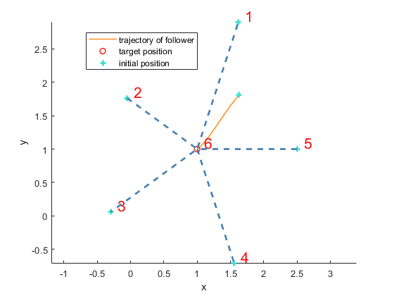
(a) System trajectories.

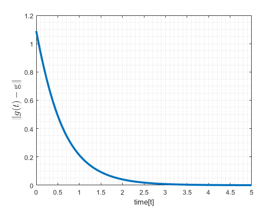
(b) Bearing error along the system trajectories.

Figure 6: A 1-to-many system with 5 leaders.

Consider $6$ agents in the one-to-many system configuration. In this example, the desired bearings are $\bm{\mathrm{g}}_{61}=[0.309,0.951]^{T}$, $\bm{\mathrm{g}}_{62}=[-0.809,0.588]^{T}$, $\bm{\mathrm{g}}_{63}=[-0.809,-0.588]^{T}$, $\bm{\mathrm{g}}_{64}=[0.309,-0.951]^{T}$, and $\bm{\mathrm{g}}_{65}=[1,0]^{T}$. The leaders are placed at $\mathrm{p}_{1}=[1.618,2.902]^{T}$, $\mathrm{p}_{2}=[-0.051,1.764]^{T}$, $\mathrm{p}_{3}=[-0.294,0.060]^{T}$, $\mathrm{p}_{4}=[1.556,-0.712]^{T}$, $\mathrm{p}_{5}=[2.500,0]^{T}$, which can be verified to satisfy Assumption 1. The initial position for the follower agent is chosen randomly as $p_{6}(0)=[1.6254,1.8106]^{T}$.

According to Proposition 1, equilibrium position for the follower agent can be calculated as

$$\mathrm{p}_{6}=\left(\sum_{j=1}^{5}P_{\bm{\mathrm{g}}_{6j}}\right)^{-1}\left(\sum_{j=1}^{5}P_{\bm{\mathrm{g}}_{6j}}\mathrm{p}_{j}\right)=\begin{bmatrix}1\\ 1\end{bmatrix}.$$

Figure 6(a) depicts the trajectory and the final position of the follower matching the analytic result. Figure 6(b) verifies that the bearing error converges to zero exponentially fast.

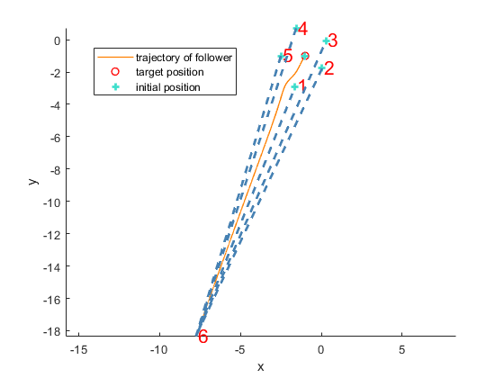
(a) System trajectories.

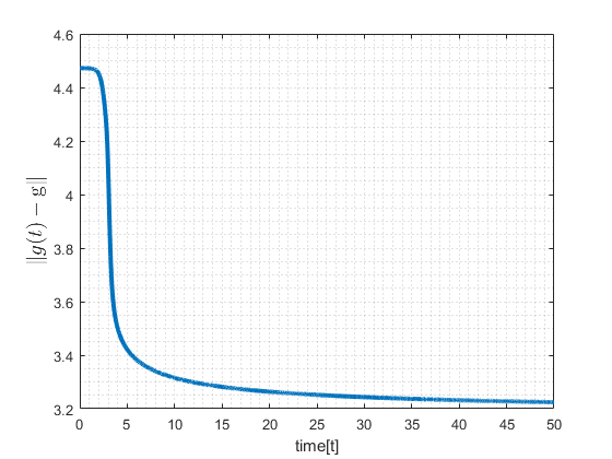
(b) Bearing error along the system trajectories.

Figure 7: 1-to-many system initialized near the unstable equilibrium.

We now consider the same setup but with initial conditions that are symmetric with respect to the origin. The leaders are placed at $\bar{p}=-[\mathrm{p}_{1}^{T},\mathrm{p}_{2}^{T},\mathrm{p}_{3}^{T},\mathrm{p}_{4}^{T},\mathrm{p}_{5}^{T}]^{T}$. From Lemma 6, the system has a unique unstable equilibria at $\mathrm{p}_{6}=[1\ 1]^{T}$. In simulation, the initial position is taken near the unstable equilibria at $p_{6}(0)=[1.01\ 1.01]^{T}$. As depicted in Fig.7, the follower diverges from the unstable equilibria, and the bearing error does not converge to zero.

IV-B Performance Improvement of Ordered LFF Graphs

In this example, we demonstrate how ordered LFF graphs lead to faster convergence to the desired formation compared to the LFF graphs used in [18].

Figure 8: The sensing graphs for the examples in Sections IV-B and IV-C. The graph with only the black edges is LFF. The graph with the black and red edges is an ordered LFF. Finally, the graph with black, red, and orange is an unordered LFF.

We consider the LFF graph in Fig.8 with black edges, and an ordered LFF graph obtained by adding the red edges. The leader node is denoted in red ($p_{1}$) and the first follower in blue ($p_{2}$).

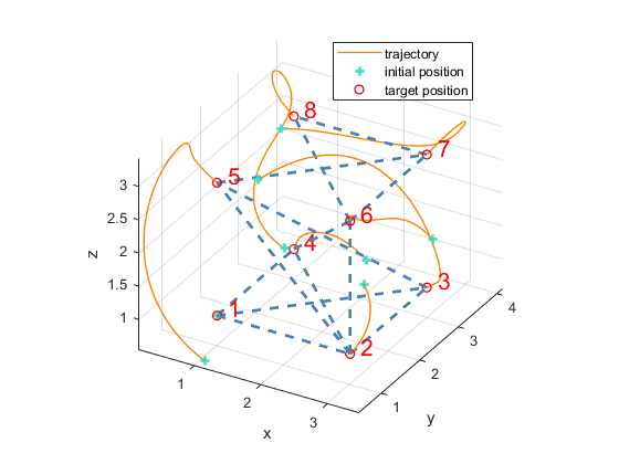
(a) BOFC with LFF graph.

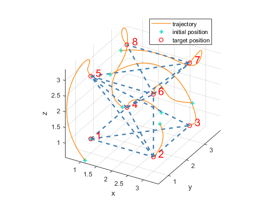
(b) BOFC with ordered LFF graph.

Figure 9: Trajectories for (a) the LFF graph, and (b) the ordered LFF graph.

Figure 9 shows the trajectories of the BOFC for the LFF (Fig. 9(a)) and ordered LFF (Fig. 9(b)) for a target formation embedded in $\mathbb{R}^{3}$. The bearing error along the trajectories for each case is displayed in Fig.10. The additional edges in the ordered LFF structure lead to a faster convergence rate to the target formation.

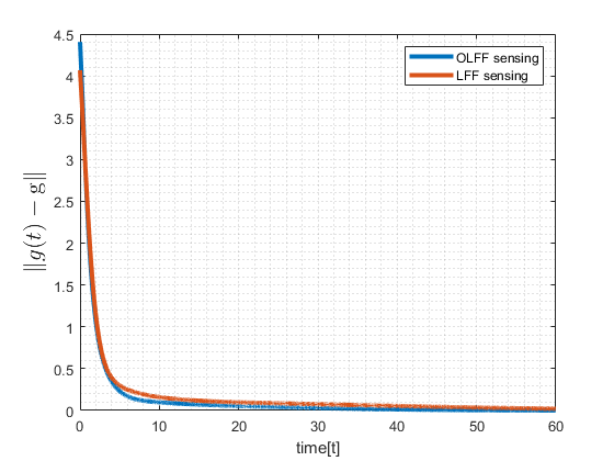
Figure 10: Caparison of bearing error along the system trajectories between the LFF and ordered LFF graphs.

IV-C Further Extensions to the LFF Graphs

Finally, we demonstrate that there are additional graph structures that may still solve the BOFC problem. We consider again the graph in Figure 8 with the black, red, and orange edges. Note that the orange edges are not forward edges, and therefore the graph is neither an LFF or ordered LFF graph. On the other hand, there is an LFF subgraph in this structure. Figure 11 shows the system trajectories and bearing error of the BOFC using this sensing graph. The fact that the system converges to the correct target formation suggests there are additional structures that demand further examination. Note that for this example, the resulting dynamics do not have a cascade structure so the methods used in this work can not apply to study its behavior. Exploring these other structures is a subject of future work.

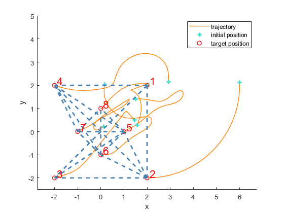
(a) System trajectory.

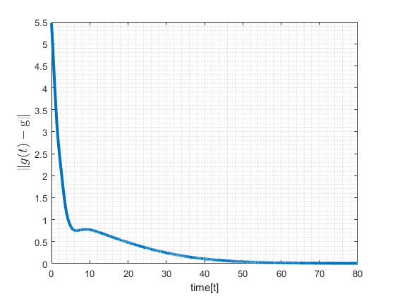
(b) Bearing error along the system trajectories.

Figure 11: Trajectories for the BOFC strategy with a graph that is neither LFF or an ordered LFF graph.

V Conclusion

This work extends the applicability of bearing-only formation control to a broader class of directed sensing graphs by augmenting traditional LFF structures. We demonstrated how forward directed edges can be added to enhance performance while preserving stability, and our simulation results highlight the improved convergence and design flexibility of the proposed methods. Future research will focus on exploring more general directed topologies, incorporating robustness to sensing uncertainties, and addressing real-world constraints, such as communication delays and dynamic network changes, to bridge the gap between theoretical advancements and practical implementations.

References

- [1] M. A. Lewis and K.-H. Tan, “High precision formation control of mobile robots using virtual structures,” Autonomous Robots, vol. 4, pp. 387–403, 1997.
- [2] W. Ren, “Consensus based formation control strategies for multi-vehicle systems,” in American Control Conference. IEEE, 2006.
- [3] D. Xu, X. Zhang, Z. Zhu, C. Chen, and P. Yang, “Behavior-based formation control of swarm robots,” Mathematical Problems in Engineering, vol. 2014, p. 1–13, 2014.
- [4] W. Ren and E. Atkins, “Distributed multi‐vehicle coordinated control via local information exchange,” International Journal of Robust and Nonlinear Control, vol. 17, no. 10–11, p. 1002–1033, Nov. 2006.
- [5] H. G. de Marina, “Maneuvering and robustness issues in undirected displacement-consensus-based formation control,” IEEE Transactions on Automatic Control, vol. 66, no. 7, p. 3370–3377, Jul. 2021.
- [6] L. Krick, M. E. Broucke, and B. A. Francis, “Stabilisation of infinitesimally rigid formations of multi-robot networks,” International Journal of Control, vol. 82, no. 3, p. 423–439, Feb. 2009.
- [7] S. Zhao and D. Zelazo, “Bearing rigidity and almost global bearing-only formation stabilization,” IEEE Transactions on Automatic Control, vol. 61, no. 5, p. 1255–1268, May 2016.
- [8] L. Chen, M. Cao, and C. Li, “Angle rigidity and its usage to stabilize multiagent formations in 2-d,” IEEE Transactions on Automatic Control, vol. 66, no. 8, pp. 3667–3681, 2021.
- [9] K.-K. Oh and H.-S. Ahn, “Formation control of mobile agents based on inter-agent distance dynamics,” Automatica, vol. 47, no. 10, p. 2306–2312, Oct. 2011.
- [10] H. Ahn, Formation Control: Approaches for Distributed Agents, ser. Studies in Systems, Decision and Control. Springer International Publishing, 2019.
- [11] S. Zhao and D. Zelazo, “Bearing rigidity theory and its applications for control and estimation of network systems: Life beyond distance rigidity,” IEEE Control Systems Magazine, vol. 39, no. 2, pp. 66–83, 2019.
- [12] J. M. Hendrickx, B. D. Anderson, J. C. Delvenne, and V. D. Blondel, “Directed graphs for the analysis of rigidity and persistence in autonomous agent systems,” International Journal of Robust and Nonlinear Control, vol. 17, no. November 2006, pp. 960–981, 2007.
- [13] M. A. Belabbas, “On global stability of planar formations,” IEEE Transactions on Automatic Control, vol. 58, no. 8, pp. 2148–2153, 2013.
- [14] R. Babazadeh and R. R. Selmic, “Distance-based formation control over directed triangulated laman graphs in 2-d space,” in IEEE Conference on Decision and Control, 2020, pp. 2786–2792.
- [15] C. Yu, B. D. O. Anderson, S. Dasgupta, and B. Fidan, “Control of minimally persistent formations in the plane,” SIAM Journal on Control and Optimization, vol. 48, no. 1, pp. 206–233, 2009.
- [16] S. Zhao and D. Zelazo, “Bearing-based formation stabilization with directed interaction topologies,” in IEEE Conference on Decision and Control. IEEE, Dec. 2015.
- [17] Z. Sun, S. Zhao, and D. Zelazo, “Characterizing bearing equivalence in directed graphs,” IFAC-PapersOnLine, vol. 56, no. 2, p. 3788–3793, 2023.
- [18] M. H. Trinh, S. Zhao, Z. Sun, D. Zelazo, B. D. O. Anderson, and H.-S. Ahn, “Bearing-based formation control of a group of agents with leader-first follower structure,” IEEE Transactions on Automatic Control, vol. 64, no. 2, pp. 598–613, 2019.
- [19] M. Mesbahi and M. Egerstedt, Graph Theoretic Methods in Multiagent Networks. Princeton University Press, Dec. 2010.
- [20] J. N. Franklin, Matrix Theory. Englewood Cliffs, N.J.: Prentice-Hall, 1968.