Sum Rate Enhancement using Machine Learning for Semi-Self Sensing Hybrid RIS-Enabled ISAC in THz Bands

Abstract

This paper proposes a novel semi- self sensing hybrid reconfigurable intelligent surface (SS- HRIS) in terahertz (THz) bands, where the RIS is equipped with reflecting elements divided between passive and active elements in addition to sensing elements. SS-HRIS along with integrated sensing and communications (ISAC) can help to mitigate the multipath attenuation that is abundant in THz bands. In our proposed scheme, sensors are configured at the SS-HRIS to receive the radar echo signal from a target. A joint base station (BS) beamforming and HRIS precoding matrix optimization problem is proposed to maximize the sum rate of communication users while maintaining satisfactory sensing performance measured by the Cramér- Rao bound (CRB) for estimating the direction of angles of arrival (AoA) of the echo signal and thermal noise at the target. The CRB expression is first derived and the sum rate maximization problem is formulated subject to communication and sensing performance constraints. To solve the complex non- convex optimization problem, deep deterministic policy gradient (DDPG)- based deep reinforcement learning (DRL) algorithm is proposed, where the reward function, the action space and the state space are modeled. Simulation results show that the proposed DDPG- based DRL algorithm converges well and achieves better performance than several baselines, such as the soft actor–critic (SAC), proximal policy optimization (PPO), greedy algorithm and random BS beamforming and HRIS precoding matrix schemes. Moreover, it demonstrates that adopting HRIS significantly enhances the achievable sum rate compared to passive RIS and random BS beamforming and HRIS precoding matrix schemes.

I Introduction

Incorporating sensing capabilities into wireless communication networks has recently emerged as an important feature in the advancement of beyond fifth-generation (B5G) as well as the sixth- generation (6G) networks [1]. To reduce the hardware costs, decrease power consumption and boost the spectral efficiency, sharing the same time-frequency resources and hardware platform between radar and communication has recently attracted research interest and attention from both the industry [2]. Furthermore, integrated sensing and communication (ISAC) allows wireless networks to gather sensory data from the surroundings, thereby contributing to the development of smart environment–aware technologies [3]. In this evolving ISAC landscape, conventional RISs have been employed to assist communication by enhancing data transmission. However, sensing–augmented RIS (SA-RIS) introduces a new role where the RIS can be deployed to assist ISAC by facilitating line-of-sight (LOS) paths for sensing tasks handled by the BS alone [4, 5]. The SA–RIS simply reflects the probing signals generated by the BS, allowing the BS to carry out target detection or environmental sensing with enhanced reach and accuracy. Moving beyond this reflective assistance, a more advanced concept, known as semi-self sensing RIS (SS–RIS), has recently been introduced to reduce the reliance on the BS for sensing tasks. Unlike SA–RIS, SS–RIS incorporates a mix of reflecting and sensing elements [6]. While the SS-RIS still depends on the BS to generate probing signals, it can directly receive echo signals from targets, allowing for basic radar sensing [7]. This semi-autonomous design reduces signal degradation associated with multi-hop paths (e.g., BS $\rightarrow$ RIS $\rightarrow$ target $\rightarrow$ RIS $\rightarrow$ BS), as it only requires a two-hop reflection (i.e., BS $\rightarrow$ RIS reflecting elements $\rightarrow$ target $\rightarrow$ RIS sensing elements) [8].

The field of SS– RIS-assisted ISAC is still in its nascent stages , with only a handful of studies available in the literature [6, 7, 9, 10]. Inspired by [6], which is the first work to propose the concept of SS– RIS, the authors in [7] explored a millimeter–wave (mmWave) ISAC system, where an SS– passive RIS is deployed to provide connectivity between the BS, communication users, and targets. In their work, a joint optimization problem is formulated on hybrid BS beamforming and RIS phase shifts to minimize the CRB, while guaranteeing good communication performance, evaluated by the achievable data rate. In [9], the authors investigated joint channel and AoA estimation in an SS– RIS- unmanned aerial vehicle (UAV) network, where the effect of the SS– RIS power splitting coefficient on the estimations of the individual channels and the AoAs of the LOS path of the UAV-RIS link is analyzed.
Additionally, since passive RIS is only capable of reflecting the incident signal with no amplification gain introduced and the capacity gain provided by passive RIS is limited due to multiplicative fading effect, HRIS is proposed. Here, some of the RIS reflecting elements are active (e.g. amplification gain introduced) and the rest are passive. This combination of active and passive RIS elements is proven to be the optimal selection to address the trade–off the system performance and hardware costs. Hence, it is a promising approach to deploy HRIS in the ISAC systems [11].
Despite several research studies, analyzing the sum rate of the ISAC downlink system through an SS– sensing HRIS has not been explored, in particular considering the THz band and the sensing performance is guaranteed. In this paper, we specifically tackle this problem by considering an SS– HRIS, equipped with both reflective (passive and active) elements and sensing elements, in an ISAC downlink network to establish LOS between the BS and the communication users (and a target) in the THz band. A DDPG–based DRL algorithm is employed to jointly optimize the BS beamforming and the HRIS precoding matrix. Our main contributions can be summarized as follows:

• A joint BS beamforming and SS– HRIS precoding matrix optimization scheme is proposed to maximize the sum rate of the scenario under consideration given the constraints of the HRIS, sensing performance measured by CRB and thermal noise sensed at the target and limited power budgets of both the BS and HRIS.

• Given the formulated sum rate maximization problem is non-convex non-trivial one, due to the non-convexity of both the objective function and the constraints, we reformulate the problem within the framework of DRL. The DDPG algorithm is utilized to derive the feasible solutions for W and $\mathbf{\Phi}$ as the outputs of the DRL neural network.

• Simulation results demonstrated that DDPG readily outperforms other benchmark algorithms, such as PPO, SAC, Greedy and random algorithms in terms of the sum rate. Moreover, HRIS is found to surpass the passive RIS and random schemes thanks to its provided substantial gains.

II System and Channel Model

II-A System Model

Consider a downlink ISAC model operating in THz band, where a BS transmits signals to serve $K$ single–antenna communication users in addition to probing signals to sense a single target. Without loss of generality, the direct links between the BS and the users, as well as that between the BS and the target, are assumed to be unattainable due to high loss caused by obstacles and long transmission distance. Consequently, an SS– HRIS is deployed, equipped with both reflecting (passive and active) elements as well as sensing elements, to establish LOS between the BS and the users (and the target). The BS is assumed to be equipped with a uniform plannar array (UPA) consisting of $M=M_{x}M_{z}$ transmit antenna elements deployed in the $x-z$ plane, the SS– HRIS can be also treated as a UPA consisting of $N=N_{y}N_{z}$ reflecting elements and $N_{s}=N_{s_{y}}N_{s_{z}}$ sensing elements deployed in the $y-z$ plane.

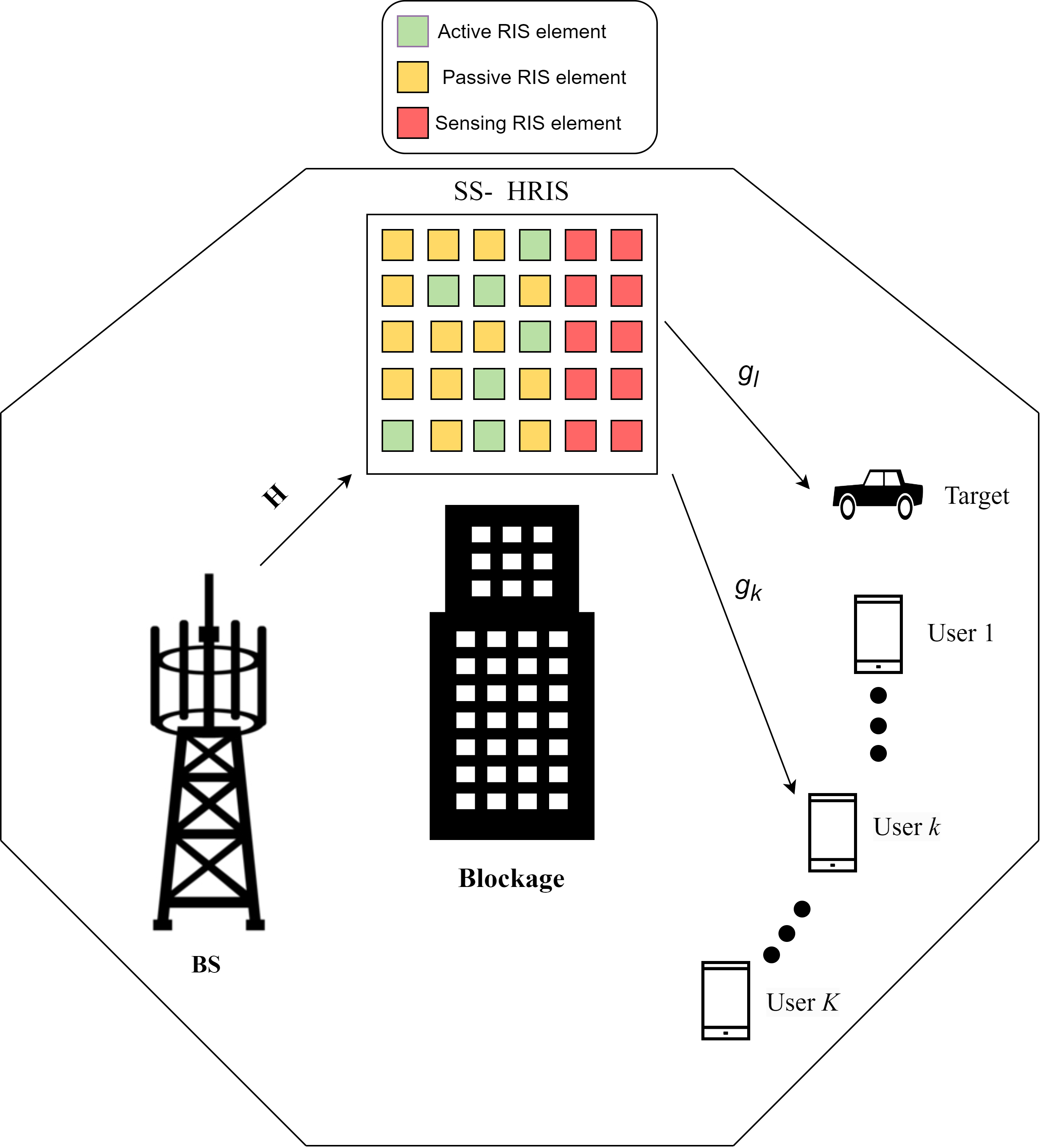
Figure 1: Scenario considering an SS– HRIS that is deployed to assist the communication link between the BS and $K$ communication users and a target.

II-B Channel Model

Consider the THz wave transmission attenuation model and water vapour absorption that primarily characterize the THz band [12, 13], the THz channel matrix between the BS and the RIS reflecting elements is expressed as

$$\textbf{H}=\sqrt{\frac{NM}{PL(f,d)}}\bm{\alpha}_{r}(\psi^{r},\omega^{r})\bm{\alpha}_{t}^{H}(\psi^{t},\omega^{t}),$$ (1)

where $PL(f,d)$ represents the pathloss experienced at frequency $f$ after propagating a distance $d$ and is given as

$$PL{(f,d)}=\Big{(}\frac{4\pi fd}{C}\Big{)}^{2}e^{k(f)d},$$ (2)

where $C$ and $k(f)$ represent the speed of light in free space and the frequency dependent medium absorption factor, respectively. Also, $\bm{\alpha}_{{\color[rgb]{0,0,0}r}}(\psi^{{\color[rgb]{0,0,0}r}},\omega^{{\color[rgb]{0,0,0}r}})$ and $\bm{\alpha}_{{\color[rgb]{0,0,0}t}}(\psi^{t},\omega^{t})$ in (1) represent RIS and BS steering vectors, which are expressed respectively as

$$\bm{\alpha}_{r}(\psi^{r},\omega^{r}) =\frac{1}{\sqrt{N}}\begin{bmatrix}1,\ldots,e^{-j\frac{2\pi}{\lambda}(N_{y}-1)\sin\psi^{r}\sin\omega^{r}d_{r}}\end{bmatrix}^{T}$$

$$\otimes\begin{bmatrix}1,\ldots,e^{-j\frac{2\pi}{\lambda}(N_{z}-1)\cos\omega^{r}d_{r}}\end{bmatrix}^{T},$$ (3a)

$$\bm{\alpha}_{t}(\psi^{t},\omega^{t}) =\frac{1}{\sqrt{M}}\begin{bmatrix}1,\ldots,e^{-j\frac{2\pi}{\lambda}(M_{x}-1)\cos\psi^{t}\sin\omega^{t}d_{b}}\end{bmatrix}^{T}$$

$$\otimes\begin{bmatrix}1,\ldots,e^{-j\frac{2\pi}{\lambda}(M_{z}-1)\cos\omega d_{b}}\end{bmatrix}^{T}.$$ (3b)

where $\psi^{r}$, $\omega^{r}$, $\psi^{t}$, $\omega^{t}$ and $d_{r}$ and $d_{b}$ denote azimuth/elevation angles of arrival/departure (AoA/AoD), the element spacing of RIS elements and transmit antenna elements at the BS. The channel from the RIS to user $k$ can be modeled in a similar manner, with only transmit array response due to a single receive antenna at users.

III Mathematical Formulation

III-A Metrics for Communications

The received signal at each communication user $k$ can be expressed as

$$\begin{aligned} y_{k}(t)=&\underbrace{\bm{g}_{k}^{H}\bm{\Phi}\bm{H}\bm{w}_{k}s_{k}(t)}_{\text{Desired Signal}}+\sum_{\begin{subarray}{c}j=1\\ j\neq i\end{subarray}}^{K}\underbrace{\bm{g}_{k}^{H}\bm{\Phi}\bm{H}\bm{w}_{j}s_{j}(t)}_{\text{ Inter- user Interference}}\\ &+\underbrace{\bm{g}_{k}^{H}\bm{A}\bm{\Phi}\bm{n}_{a}}_{\text{Dynamic Noise}}+\underbrace{\bm{g}_{l}^{H}\bm{\Phi}\bm{H}\bm{w}_{K+1}s_{K+1}(t)}_{\text{Sensing Interference}}+\underbrace{n_{o}}_{\text{AWGN}},\end{aligned}$$ (4)

where $\bm{g}_{k}\in\mathbb{C}^{N\times 1}$ denotes the channel vector between the HRIS and communication user $k$, $\bm{\Phi}\in\mathbb{C}^{N\times N}$ denotes the precoding matrix of the HRIS coefficients (i.e., phase shifts and amplitudes), where $\bm{\Phi}$ = diag [$\eta_{1}e^{j\theta_{1}},...,\eta_{N}e^{j\theta_{N}}]^{H}$ and $\theta_{n}\in[\ 0,2\pi$) and $\bm{H}\in\mathbb{C}^{N\times M}$ is the channel matrix between the UPA of the BS and the HRIS. We define $\bm{W}=[\bm{w}_{1},....,\bm{w}_{K+1}]$, where $\bm{w}_{k}\in\mathbb{C}^{M\times 1}$ is the BS beamforming for user $k$, $\bm{s}(t)\in\mathbb{C}^{K+1\times 1}$ represents the transmit data symbol that consists of $K$ data streams for serving the $K$ communication users and one stream for the sensing target such as $\bm{s}(t)=[\underbrace{s_{1}(t),...,s_{K}(t)}_{Communication},\underbrace{s_{K+1}(t)}_{Sensing}]^{T}$. Also, $\bm{A}$ is defined as a selection matrix represented as a diagonal matrix with a total of $q$ ones in its diagonal, where $q$ represents the number of active elements in the HRIS which are randomly assigned, $\bm{n}_{a}\sim CN(0,\sigma_{a}^{2}\bm{I_{N}})$ represents the dynamic noise generated by the active elements, which is related to the input noise as well as inherent device noise of active RIS elements [14], and $n_{o}$ denotes the additive white Gaussian noise (AWGN) which has zero mean and variance $\sigma_{o}^{2}$.

According to (4), the achieved SINR at the communication user $k$ can be given by

$$\begin{aligned} &\gamma_{k}=\\ &\frac{|\bm{g}_{k}^{H}\bm{\Phi}\bm{H}\bm{w}_{k}|^{2}}{\sum_{\begin{subarray}{c}j=1\\ j\neq i\end{subarray}}^{K}|\bm{g}_{k}^{H}\bm{\Phi}\bm{H}\bm{w}_{j}|^{2}+|\bm{g}_{l}^{H}\bm{\Phi}\bm{H}\bm{w}_{K+1}|^{2}+||\bm{g}_{k}^{H}\bm{A}\bm{\Phi}||^{2}\sigma_{a}^{2}+\sigma_{o}^{2}}.\end{aligned}$$ (5)

Accordingly, the achievable data rate of user $k$ is expressed as

$$R_{k}=\log_{2}(1+\gamma_{k}).$$ (6)

III-B Metrics for Sensing

As for the target, we assume it is in the far field of the BS and the SS– HRIS so that it can be viewed as a point–like target. As such, the steering vectors of the HRIS sensing elements and reflecting elements can be expressed respectively as

$$\bm{\alpha}(\psi,\omega) =\frac{1}{\sqrt{N_{s}}}\left[\begin{array}[]{c}1,\dots,e^{-j\frac{2\pi}{\lambda}(N_{sy}-1)\sin\psi\sin\omega d_{y}}\end{array}\right]^{T}$$ (7b)

$$\otimes\left[\begin{array}[]{c}1,\dots,e^{-j\frac{2\pi}{\lambda}(N_{sz}-1)\cos\omega d_{z}}\end{array}\right]^{T},$$ (7d)

$$\bm{\beta}(\psi,\omega) =\frac{1}{\sqrt{N}}\left[\begin{array}[]{c}1,\dots,e^{-j\frac{2\pi}{\lambda}(N_{y}-1)\sin\psi\sin\omega d_{y}}\end{array}\right]^{T}$$ (7f)

$$\otimes\left[\begin{array}[]{c}1,\dots,e^{-j\frac{2\pi}{\lambda}(N_{z}-1)\cos\omega d_{z}}\end{array}\right]^{T},$$ (7h)

where $\lambda$ denotes the carrier wavelength, and $d_{y}$ and $d_{z}$ denote the horizontal and vertical adjacent HRIS element spaces, respectively, and $\psi$ and $\omega$ are the azimuth and elevation angles.
In addition, the received echo signal from the target at the sensors of the HRIS can be expressed as

$$\begin{aligned} \bm{Y}_{target}=&\rho\bm{\alpha}(\psi,\omega)\bm{\beta}^{T}(\psi,\omega)\bm{\Phi}\bm{H}\bm{X}\\ +&\rho\bm{\alpha}(\psi,\omega)\bm{\beta}^{T}(\psi,\omega)\bm{\Phi}\bm{N}_{a}+\bm{N_{o}},\end{aligned}$$ (8)

where $\rho$ represents a complex constant counting for the round–trip pathloss as well as the radar cross section (RCS) at the target, $d_{y}$ and $d_{z}$ represent the horizontal and vertical adjacent RIS elements spacing, $\mathbf{N}_{a}$ denotes the HRIS dynamic noise with each entry being $\sigma_{a}^{2}$, and $\mathbf{N}_{o}$ denotes the AWGN with each entry being $\sigma_{o}^{2}$. Assume that the fluctuations of the RCS are slow and the round–trip sensing channel is unchanged during the transmission of $T$ communication and sensing symbols, where the Swerling–I model is applicable [15]. From (8), it is noted that the transmitted signal, received signal, and the AWGN are stacked as $\mathit{\mathbf{X}}=[\mathit{\mathbf{x}}(1),\ldots,\mathit{\mathbf{x}}(T)]$, $\mathit{\mathbf{Y}}_{target}=[\mathit{\mathbf{y}}_{target}(1),\ldots,\mathit{\mathbf{y}}_{target}(T)]$ and $\mathit{\mathbf{N}}_{o}=[\mathit{\mathbf{n}}_{o}(1),\ldots,\mathit{\mathbf{n}}_{o}(T)]$, respectively, where $T$ also represents the radar dwell time. When $T$ is very large, the covariance matrix of the transmit signal $\mathbf{x}(t)$ can be written as:

$$\textbf{R}_{\mathbf{x}}=\mathbb{E}\{\mathbf{x}(t)\mathbf{x}^{H}(t)\}=\textbf{W}\textbf{W}^{H}\approx\frac{1}{T}\textbf{X}\textbf{X}^{H}.$$ (9)

As such, $\textbf{Y}_{target}$ is vectorized so that the following holds [7]

$$\textbf{y}_{target}=vec(\mathbf{Y}_{target})=\textbf{b}+\textbf{n}_{o},$$ (10)

where

$$\textbf{b}=\text{vec}\left({\rho}\bm{\alpha}(\psi,\omega)\bm{\beta}^{H}(\psi,\omega)\bm{\Phi}\mathbf{H}\mathbf{X}+\rho\bm{\alpha}(\psi,\omega)\bm{\beta}^{H}(\psi,\omega)\bm{\Phi}\mathbf{N}_{a}\right),$$ (11a)

$$\textbf{n}_{o}=\text{vec}(\mathbf{N}_{o})\in\mathcal{CN}(0,\mathbf{R}_{\mathbf{n}_{o}}),\quad\mathbf{R}_{\mathbf{n}_{o}}=\sigma_{o}^{2}\mathbf{I}_{N_{s}T}.$$ (11b)

Let the estimated parameters for target sensing $\tilde{\bm{\epsilon}}=$ [$\tilde{\bm{\xi}}^{T}$,$\textbf{$\tilde{\bm{\rho}}$}^{T}$]^T, where $\tilde{\bm{\xi}}$ = [$\psi$,$\omega$]^T and $\tilde{\bm{\rho}}$ = [$\Re$$\{\rho\}$ + $\Im{\{\rho\}}]^{T}$.
Hence, the fisher information matrix (FIM) for estimating parameter $\tilde{\bm{\epsilon}}$ can be generally written as

$$\mathbf{J}=\begin{bmatrix}\mathbf{J_{\tilde{\bm{\xi}}\tilde{\bm{\xi}}}}&\mathbf{J_{\tilde{\bm{\xi}}\tilde{\bm{\rho}}}}\\ \mathbf{J_{\tilde{\bm{\xi}}\tilde{\bm{\rho}}}}^{T}&\mathbf{J_{\tilde{\bm{\rho}}\tilde{\bm{\rho}}}}\end{bmatrix},$$ (12)

where each element of J can be written as

$$\mathbf{J}_{i,j} =\text{tr}\left(\mathbf{R}_{\mathbf{n}_{o}}^{-1}\frac{\partial\mathbf{R}_{\mathbf{n}_{o}}}{\partial\tilde{\mathbf{\tilde{\bm{\epsilon}}}}_{i}}\mathbf{R}_{\mathbf{n}_{o}}^{-1}\frac{\partial\mathbf{R}_{\mathbf{n}_{o}}}{\partial\tilde{\mathbf{\tilde{\bm{\epsilon}}}}_{j}}\right)\quad+2\Re\left\{\frac{\partial\textbf{b}^{H}}{\partial\tilde{\mathbf{\tilde{\bm{\epsilon}}}}_{i}}\mathbf{R}_{\mathbf{n}_{o}}^{-1}\frac{\partial\textbf{b}}{\partial\tilde{\mathbf{\tilde{\bm{\epsilon}}}}_{j}}\right\}$$

$$\overset{\text{(a)}}{=}\frac{2}{\sigma_{o}^{2}}\Re\left\{\frac{\partial\textbf{b}^{H}}{\partial\tilde{\mathbf{\tilde{\bm{\epsilon}}}}_{i}}\frac{\partial\textbf{b}}{\partial\tilde{\mathbf{\tilde{\bm{\epsilon}}}}_{j}}\right\}.$$ (13)

This is because $\textbf{R}_{\textbf{n}_{o}}$ is independent of $\mathbf{\tilde{\bm{\epsilon}}}$ such that $\frac{\partial\textbf{R}_{\textbf{n}_{o}}}{\partial\tilde{\bm{\epsilon}_{i}}}=0$ for any $i$. The derivation of the FIM elements is provided in Appendix A. Furthermore, the CRB for estimating $\tilde{\bm{\xi}}$ is given as

$$\text{CRB}(\tilde{\bm{\xi}})=\left[\textbf{J}_{\tilde{\bm{\xi}}\tilde{\bm{\xi}}}-\textbf{J}_{\tilde{\bm{\xi}}\tilde{\bm{\rho}}}\textbf{J}_{\tilde{\bm{\xi}}\tilde{\bm{\rho}}}^{-1}\textbf{J}_{\tilde{\bm{\xi}}\tilde{\bm{\rho}}}^{T}\right]^{-1}.$$ (14)

Assuming that the target moves slowly, the target direction does not change remarkably over the adjacent coherent time slots. Accordingly, the predicted angles are enough for the waveform optimization that is necessary for minimizing the CRB. This is a typical scenario in radar tracking, where prior knowledge of the target direction is well-known for system design [7]. Thus, the target angle $\mathbf{\tilde{\bm{\xi}}}$ is assumed to be fixed in this study.

III-C Optimization Problem Formulation

The sum rate maximization problem can be formulated as

$$\max_{\textbf{W},\mathbf{\Phi}} \quad\sum_{k=1}^{K}R_{k}$$ (15a)

subject to:

$$\gamma_{k} \geq\gamma_{\text{th}},\quad\forall k\in K,$$ (15b)

$$\text{tr}(\textbf{W}\textbf{W}^{H}) \leq P_{\text{BS}}^{\text{max}},$$ (15c)

$$E\left[\|\textbf{A}\mathbf{\Phi}(\textbf{H}\textbf{x}+\textbf{n})\|^{2}\right] \leq P_{\text{RIS}}^{\text{max}},$$ (15d)

$$\|\textbf{g}_{l}^{H}\mathbf{A}\mathbf{\Phi}\|^{2}\sigma_{2}^{2} \leq r_{\text{max}},$$ (15e)

$$|\theta_{i}| \leq\begin{cases}1,&\forall i\notin\mathcal{A},\\ P_{A,\text{max}},&\forall j\in\mathcal{A},\end{cases}$$ (15f)

$$\text{CRB}(\textbf{W},\mathbf{\Phi}) \leq\text{CRB}_{\text{max}}.$$ (15g)

where (15b) ensures the minimum SINR for communication users. (15c) and (15d) represent the total power budgets dedicated for the BS and the HRIS, respectively. (15e) limits the thermal noise received at the the target within a certain range. (15f) imposes an amplitude constraint on HRIS. (15g) limits the CRB for the target estimation accuracy.

IV DRL–Based Joint Design of BS Beamforming and HRIS Precoding Matrix

Since the objective function and the constraints in (15) are non–convex leading to a non–convex non–trivial optimization problem, obtaining the optimal solution by utilizing classical mathematical tools would be impossible to achieve, specially for large scale network. In our work, rather than directly solving the challenging optimization problem mathematically, we formulate the sum rate optimization problem in the context of DDPG–based DRL method to obtain the feasible BS beamforming W and the HRIS precoding matrix $\mathbf{\Phi}$.

IV-A Proposed MDP

The state and action spaces, and the reward that are used to represent our joint BS beamforming and HRIS precoding matrix optimization problem are designed as follows:

• State: The state vector $\mathbf{s}^{(t)}$ is composed of the current values of the BS beamforming matrix $\mathbf{W}\in\mathbb{C}^{M\times K+1}$, the current values of the elements in the main diagonal of the HRIS precoding matrix, i.e., in the vector $Diag(\bm{\Phi})\in\mathbb{C}^{N\times 1}$, the elements in the matrix $\mathbf{H}\in\mathbb{C}^{N\times M}$ that stacks the channel gains from the BS to the HRIS, and the elements in the matrix $\textbf{G}\in\mathbb{C}^{K+1\times N}$ that represent the channel gains from the HRIS to the $K$ users and the target such as $\textbf{G}=[\bm{g}_{1},....,\bm{g}_{K},\bm{g}_{l}]$. Since the real and imaginary parts of complex-valued numbers can be treated as independent inputs, the actual dimension of the state space is $D_{\text{state}}=2M(K+1)+2N+2NM+2N(K+1)$. The state is constructed such that:

  $$\mathbf{s}^{(t)}=\{ \mathbf{H}^{(t)},\mathbf{G}^{(t)},\mathbf{W}^{(t)},diag(\bm{\Phi}^{(t)})\}.$$ (16)

• Action: The action is simply constructed by the BS beamforming W and the HRIS precoding matrix $\mathbf{\Phi}$. Likewise, to deal with the real input problem, $\textbf{W}=\Re{(\textbf{W})}+\Im{(\textbf{W})}$ and $\mathbf{\Phi}=\Re{(\mathbf{\Phi})}+\Im{(\mathbf{\Phi})}$ are separated as real and imaginary parts, both are entries of the action. Hence, the dimension of the action space is $D_{a}=2M(K+1)+2N$ and the action space is constructed such as:

  $$\mathbf{a}^{(t)}=\{ \mathbf{W}^{(t)},diag(\bm{\Phi}^{(t)})\}.$$ (17)

• Reward: At the $t^{th}$ timestep of the DRL, the reward is determined as the sum rate $r(\textbf{H}^{(t)},\textbf{G}^{(t)},\textbf{W}^{(t)},diag(\bm{\Phi}^{(t)})$, given the instantaneous channels $\textbf{H}^{(t)}$ and $\textbf{G}^{(t)}$ and the action $\textbf{W}^{(t)}$ and $\mathbf{\Phi}^{(t)}$ obtained from the actor network.

  1 Initial state $s_{0}$, max episodes $E$, max steps per episode $T_{s}$, actor and critic networks, replay buffer $\mathcal{D}$, Network parameters (e.g. max amplitude $A_{max}$, max power $P_{max}$, BS Beamforming W, HRIS precoding matrix $\bm{\Phi}$, $\textbf{G},\textbf{H}$,….etc);

  2 Set initial state $s^{(t)}\leftarrow\text{normalize}(s_{0}^{(t)})$;

  3 for episode $i=1$ to $E$ do

  4    Reset environment to initial state $s^{(t)}\leftarrow\text{normalize}(s_{0}^{(t)})$;

  5    for timestep $t=1$ to $T_{s}$ do

  6       Select action $a^{(t)}$ using actor network;

  7       $a^{(t)}\leftarrow\text{scale\_actions}(a^{(t)},A_{max},P_{max})$;

  8       Execute action $a_{t}$, observe reward $r_{t}$ and next state $s^{(t+1)}$;

  9       $s^{(t+1)}\leftarrow\text{normalize}(s^{(t+1)})$;

  10       Store transition $(s^{(t)},a^{(t)},r^{(t)},s^{(t+1)})$ in replay buffer $\mathcal{D}$;

  11       Sample mini-batch from replay buffer $\mathcal{D}$;

  12       Update critic network by minimizing loss;

  13       Update actor network using policy gradient;

  14       Apply penalties if constraints in (15) are violated;

  15       Set $s^{(t)}\leftarrow s^{(t+1)}$;

  16      

  17   if constraints in (15) are met or max timesteps reached then

  18       End episode;

  19      

  20   

  21return Optimized BS beamforming matrix $\mathbf{W}_{opt}$ and HRIS precoding matrix $\bm{\Phi}_{opt}$;

  Algorithm 1 DDPG for Joint BS Beamforming and HRIS Precoding Matrix Optimization

IV-B Algorithm

In this sub–section, the proposed DRL–based algorithm for joint design of the BS beamforming and the HRIS precoding matrix is presented using the DDPG neural network. We assume there exists a central controller, or the agent, which is able to instantaneously collect the channel state information (CSI), $\mathbf{G}$ and $\mathbf{H}$. At time step $t$, given the CSI and the action $\mathbf{W}^{(t-1)}$ and $\mathbf{\Phi}^{(t-1)}$ in the previous state, the agent constructs the state $\mathbf{s}^{(t)}$ for time step $t$ following sub–section III.B.

At the beginning of the algorithm, the experience replay buffer $\mathcal{D}$, the critic network and the actor network parameters, the action $\mathbf{W}$ and $\mathbf{\Phi}$ need to be initialized. In this paper, we simply adopt the identity matrix to initialize $\mathbf{W}$ and $\mathbf{\Phi}$.

Our algorithm is run over $E$ episodes, where every episode iterates $T_{s}$ steps. For each episode, the algorithm terminates whenever constraints (15b), (15c), (15d), (15e) and (15f), (15g) are met or the algorithm reaches the maximum number of allowable time steps per episode. The optimal BS beamforming $\mathbf{W}_{opt}$ and HRIS precoding $\mathbf{\Phi}_{opt}$ are obtained as the action with the best instant reward. The details of the proposed method are shown in Algorithm 1.

TABLE I: Simulation Parameters.

Parameter	Description	Value
$E$	Number of Episodes	$10$
$n_{s}$	Number of time steps per episode	$100$
$B$	Min–batch size	$100$
$\gamma_{d}$	Discount factor	$0.99$
$\gamma_{d}$	Soft update rate for target networks	$0.005$
$lr$	Learning rate	$10^{-4}$
$n_{1}$, $n_{2}$	Neural Network Dimension	{64,64}
$f$	Operating frequency	$0.2$ THz
$k(f)$	Absorption coefficient	$0.01$
$M$	Number of BS antennas	64
$N$	Number of RIS reflecting elements	80
$q$	Number of RIS active elements	30
$N_{s}$	Number of RIS sensing elements	20
$K$	Number of users	$3$
$l$	Number of Targets	$1$
$A_{max}$	Maximum amplitude of active RIS elements	5
$CRB_{max}$	Maximum CRB allowed	$10^{-3}$
$\sigma_{o},\sigma_{a}^{2}$	Noise variance	$-90$ dBm
$P_{\text{BS}}^{\text{max}}$	BS Power Budget	$30$ dBm
$P_{\text{RIS}}^{\text{max}}$	RIS Power Budget	$10$ dBm

V Simulations Results

In this section, we aim to demonstrate the performance of the proposed DDPG approach for jointly optimizing the BS beamforming and the HRIS precoding matrix for the sake of maximizing the sum rate. The environment settings and model parameters used in these simulations are detailed in Table 1.
To verify the effectiveness of our proposed scheme, we select four benchmark algorithms: random BS beamforming and HRIS phase shifts, greedy algorithm, PPO and SAC. These benchmarks provide a comprehensive comparison across different approaches to the joint BS beamforming and HRIS precoding matrix optimization. The random BS beamforming and HRIS precoding matrix scheme serves as a non–optimized baseline, while greedy algorithm represents an efficient heuristic based algorithm that may not reach globally optimal results. The PPO and SAC algorithms are included for direct comparisons as other ML baselines.

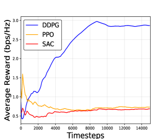
Figure 2: Average Reward vs. Timesteps for Different Algorithms.

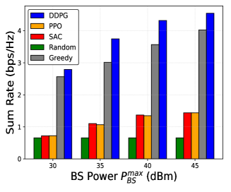
Figure 3: Average Sum Rate vs. BS Power (dBm).

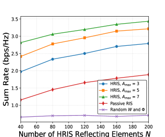
Figure 4: Average Sum Rate vs. the Number of HRIS reflecting elements for Passive RIS, Random BS Beamforming W and HRIS Precoding Matrix $\bm{\Phi}$ schemes and the proposed HRIS scheme at different values of maximum amplitude of active HRIS elements $A_{max}$.

Fig.2 shows the convergence of the average reward over iterations for DDPG, PPO and SAC. The three algorithms successfully converge, but DDPG consistently achieves the highest rewards outperforming other ML algorithms. This proves the effectiveness and superiority of optimizing the BS bemforming and HRIS precoding matrix using the DDPG in such SS– HRIS-assisted ISAC scenario.

Fig.3 shows the sum rate as a function of the BS power budget for various algorithms. As the BS power budget increases, DDPG consistently achieves the highest sum rate proving its robustness in improving the sum rate under varying power levels, followed by the greedy algorithm which still performs well but lags DDPG. At low BS power values, such as 30 dBm, PPO, SAC and random approach perform relatively similarly. As the BS power increases further, both SAC and PPO outperforms the random scheme indicating the importance of structured decision-making for better performance.

Fig.4 illustrates the effect of the number of reflecting elements $N$ on the sum rates of different schemes with BS power $P_{max}=30$ dBm and RIS sensing elements $N_{s}=20$ using DDPG, where the number of active RIS elements is set as $\left\lceil\frac{N}{4}\right\rceil$. It is readily observed that for both the HRIS and the passive RIS, the sum rates increase with $N$ thanks to the enhanced spatial degrees of freedom (DoFs) of RIS. Additionally, the HRIS schemes yields a significantly higher achievable sum rate compared to the passive RIS scheme, especially at higher values of maximum amplitude of active HRIS elements $A_{max}$. This is owing to the HRIS capabilities of providing power amplification gain and passive beamforming gain simultaneously. However, due to the limited amplification power at the HRIS, it is noticed that the sum rate achieved by the HRIS scheme increases slowly when $N$ becomes relatively large.

VI Conclusions

In this paper, we adapted an SS– HRIS downlink scenario, where the HRIS is capable of both reflecting incident signals as well as sensing the received radar echo signal from a target. The joint BS beamforming and HRIS precoding matrix optimization problem is proposed for the sake of maximizing the sum rate of communication users while guaranteeing the target accuracy estimation measured by the CRB and thermal noise. Our optimization problem is solved using the policy–based DDPG derived from Marcov decision process to optimize continuous BS beamforming matrix and HRIS precoding matrix. Through comprehensive simulations, we have demonstrated that DDPG significantly outperforms other benchmark algorithms, such as PPO, SAC, Greedy and random algorithms. Additionally, our analysis confirmed that HRIS when combined with an increased number of RIS elements, provides substantial gains compared to passive RIS and random BS beamforming and HRIS precoding matrix schemes.

Appendix A: Derivation of Fisher Information Matrix for the Point Target

From (III-B), the partial derivatives of $\mathbf{b}$ with respect to $\tilde{\bm{\xi}}$ and $\tilde{\bm{\rho}}$ are expressed as follows:

$$\frac{\partial\textbf{b}}{\partial\tilde{\mathbf{\tilde{\bm{\xi}}}}}=\left[\rho vec{(\hat{\mathbf{\Omega}}_{\psi}\Phi\mathbf{H}\mathbf{X}+\hat{\mathbf{\Omega}}_{\psi}\Phi\mathbf{N}_{a})},\rho vec{(\hat{\mathbf{\Omega}}_{\omega}\Phi\mathbf{H}\mathbf{X}+\hat{\mathbf{\Omega}}_{\omega}\Phi\mathbf{N}_{a})}\right]$$ (21)

$$\frac{\partial\textbf{b}}{\partial\tilde{\mathbf{\bm{\rho}}}}=\left[1,j\right]\otimes vec{(\mathbf{\Omega}\Phi\mathbf{H}\mathbf{X}+\mathbf{\Omega}\Phi\mathbf{N}_{a})}$$ (22)

where $\mathbf{\Omega}=\mathbf{\bm{\alpha}}(\psi,\omega)\mathbf{\bm{\beta}}^{T}(\psi,\omega)$. In order to derive the partial derivatives of $\mathbf{\Omega}$ with respect to $\psi$ and $\omega$ (denoted as $\hat{\mathbf{\Omega}}_{\psi}$ and $\hat{\mathbf{\Omega}}_{\omega}$), the steering vectors can be rewritten as:

$$\mathbf{\bm{\alpha}}(\psi,\omega)=\frac{1}{\sqrt{N_{s}}}e^{-j\bm{\delta}_{s}},\quad\mathbf{\bm{\beta}}(\psi,\omega)=\frac{1}{\sqrt{N}}e^{-j\bm{\delta}}$$ (23)

where

$$\bm{\delta}_{s} =\left[\frac{2\pi}{\lambda}\right](\kappa_{sY}\sin\psi\sin\omega d_{y}+\kappa_{sZ}\cos\omega d_{z}),$$ (24)

$$\bm{\delta} =\left[\frac{2\pi}{\lambda}\right](\kappa_{Y}\sin\psi\sin\omega d_{y}+\kappa_{Z}\cos\omega d_{z})$$ (25)

where $\kappa_{sY}$ and $\kappa_{sZ}$ denote the element indices of sensing elements at Y and Z axes, respectively, and $\kappa_{Y}$ and $\kappa_{Z}$ denote those of reflecting elements. Hence, the partial derivatives of $\mathbf{\Omega}$ can be written as:

$$\hat{\mathbf{\Omega}}_{\psi}=\frac{-2j\pi}{\lambda\sqrt{N_{s}N}}\cos\psi\sin\omega d_{y}\left(\text{diag}\{\kappa_{sY}\}\mathbf{\bm{\alpha}}\mathbf{\bm{\beta}}^{T}+\mathbf{\bm{\alpha}}\mathbf{\bm{\beta}}^{T}\text{diag}\{\kappa_{Y}\}\right)$$

$$\hat{\mathbf{\Omega}}_{\omega}= \frac{-2j\pi}{\lambda\sqrt{N_{s}N}}\sin\psi\cos\omega d_{y}\left(\text{diag}\{\kappa_{sY}\}\mathbf{\bm{\alpha}}\mathbf{\bm{\beta}}^{T}+\mathbf{\bm{\alpha}}\mathbf{\bm{\beta}}^{T}\text{diag}\{\kappa_{Y}\}\right)$$

$$\quad+ j\frac{2\pi}{\lambda\sqrt{N_{s}N}}\sin\psi d_{z}\left(\text{diag}\{\kappa_{sZ}\}\mathbf{\bm{\alpha}}\mathbf{\bm{\beta}}^{T}+\mathbf{\bm{\alpha}}\mathbf{\bm{\beta}}^{T}\text{diag}\{\kappa_{Z}\}\right)$$

With $\hat{\mathbf{\Omega}}_{\psi}$ and $\hat{\mathbf{\Omega}}_{\omega}$, the FIM elements $\mathbf{J}_{\tilde{\bm{\xi}}\tilde{\bm{\xi}}}$, $\mathbf{J}_{\tilde{\bm{\xi}}\tilde{\bm{\rho}}}$ and $\mathbf{J}_{\tilde{\bm{\rho}}\tilde{\bm{\rho}}}$ are expressed in (18), (Acknowledgment) and (20), respectively, at the top of the page.

References

- [1] S. Lu, F. Liu, Y. Li, K. Zhang, H. Huang, J. Zou, X. Li, Y. Dong, F. Dong, J. Zhu et al., “Integrated sensing and communications: Recent advances and ten open challenges,” IEEE Internet of Things Journal, 2024.
- [2] B. Zhao, C. Ouyang, X. Zhang, and Y. Liu, “Performance analysis of near-field isac based on an accurate channel model,” in ICC 2024-IEEE International Conference on Communications. IEEE, 2024, pp. 4918–4923.
- [3] Y. Cui, F. Liu, C. Masouros, J. Xu, T. X. Han, and Y. C. Eldar, “Integrated sensing and communications: Background and applications,” in Integrated Sensing and Communications. Springer, 2023, pp. 3–21.
- [4] P. Saikia, K. Singh, W.-J. Huang, and T. Q. Duong, “Hybrid deep reinforcement learning for enhancing localization and communication efficiency in ris-aided cooperative isac systems,” IEEE Internet of Things Journal, 2024.
- [5] X. Gan, C. Huang, Z. Yang, C. Zhong, X. Chen, Z. Zhang, Q. Guo, C. Yuen, and M. Debbah, “Bayesian learning for double-ris aided isac systems with superimposed pilots and data,” IEEE Journal of Selected Topics in Signal Processing, 2024.
- [6] X. Shao, C. You, W. Ma, X. Chen, and R. Zhang, “Target sensing with intelligent reflecting surface: Architecture and performance,” IEEE Journal on Selected Areas in Communications, vol. 40, no. 7, pp. 2070–2084, 2022.
- [7] W. Lyu, S. Yang, Y. Xiu, Y. Li, H. He, C. Yuen, and Z. Zhang, “Crb minimization for ris-aided mmwave integrated sensing and communications,” IEEE Internet of Things Journal, 2024.
- [8] X. Shao, C. You, and R. Zhang, “Intelligent reflecting surface aided wireless sensing: Applications and design issues,” IEEE Wireless Communications, 2024.
- [9] J. He, A. Fakhreddine, and G. C. Alexandropoulos, “Joint channel and direction estimation for ground-to-uav communications enabled by a simultaneous reflecting and sensing ris,” in ICASSP 2023-2023 IEEE International Conference on Acoustics, Speech and Signal Processing (ICASSP). IEEE, 2023, pp. 1–5.
- [10] X. Shao and R. Zhang, “Target-mounted intelligent reflecting surface for secure wireless sensing,” IEEE Transactions on Wireless Communications, 2024.
- [11] W. Hao, Y. Qu, S. Zhou, F. Wang, Z. Lu, and S. Yang, “Joint beamforming design for hybrid ris-assisted mmwave isac system relying on hybrid precoding structure,” IEEE Internet of Things Journal, 2024.
- [12] H. Zhang, H. Zhang, W. Liu, K. Long, J. Dong, and V. C. Leung, “Energy efficient user clustering, hybrid precoding and power optimization in terahertz mimo-noma systems,” IEEE Journal on Selected Areas in Communications, vol. 38, no. 9, pp. 2074–2085, 2020.
- [13] A.-A. A. Boulogeorgos, E. N. Papasotiriou, J. Kokkoniemi, J. Lehtomaeki, A. Alexiou, and M. Juntti, “Performance evaluation of thz wireless systems operating in 275-400 ghz band,” in 2018 IEEE 87th vehicular technology conference (VTC Spring). IEEE, 2018, pp. 1–5.
- [14] Z. Zhang, L. Dai, X. Chen, C. Liu, F. Yang, R. Schober, and H. V. Poor, “Active ris vs. passive ris: Which will prevail in 6g?” arXiv preprint arXiv:2103.15154, 2021.
- [15] J. Eaves and E. Reedy, Principles of modern radar. Springer Science & Business Media, 2012.