The algebraic structure of Dyson–Schwinger equations with multiple insertion places

Abstract.

We give combinatorially controlled series solutions to Dyson–Schwinger equations with multiple insertion places using tubings of rooted trees and investigate the algebraic relation between such solutions and the renormalization group equation.

1. Introduction

We explain the algebraic structure of Dyson–Schwinger equations with multiple insertion places, giving nice, combinatorially controlled expansions for the solutions of multiple insertion place Dyson–Schwinger equations in terms of tubings of rooted trees with both vertex and edge decorations. Along the way we give an algebraic formulation of the renormalization group equation and resolve a conjecture from [24]. The results are purely algebraic and combinatorial, some of independent interest for researchers in combinatorial Hopf algebras and related areas. Many of these results first appeared in the PhD thesis of one of us [25].

The reader who is not concerned with the physics motivation for these results can skip the rest of this section as well as the first half of Section 3.1.

To calculate physical amplitudes in perturbative quantum field theory it suffices to understand the renormalized one-particle irreducible (1PI) Green functions in the theory. As series one can obtain the 1PI Green functions by applying renormalized Feynman rules to sums of Feynman graphs. Choosing an external scale parameter $L$ we can think of the Green functions as multivariate series $G(x,L,\theta)$ where $x$ is the perturbative expansion parameter, for us the coupling constant, and the $\theta$ are dimensionless parameters capturing the remaining kinematic dependence. Dyson–Schwinger equations are coupled integral equations relating the Green functions, the quantum analogues of the equations of motion.

One of us has a long-standing program to find simple combinatorial understandings of the series solutions to Dyson–Schwinger equations. These first took the form of chord diagram expansions [23, 13, 20, 14, 12] and have been recently improved with the new language of tubing expansions by both of us with other authors [4].

These combinatorial solutions to Dyson–Schwinger equations stand in contrast to the Feynman diagram expansions of the Green functions because rather than each Feynman diagram contributing a difficult and algebraically opaque object (its renormalized Feynman integral) each chord diagram or tubing contributes some monomials in the coefficients of the Mellin transforms of the primitive diagrams which drive the Dyson–Schwinger equation and these monomials can be readily read off combinatorially from the chord diagram or tubing. The tubing expansion has additional benefits: Its origin is algebraic and insightful, coming from the renormalization Hopf algebra and explaining how the original Feynman diagrams map to tubings. It readily generalizes beyond the cases previously solved by chord diagrams [4]. It provides insightful structure for exploring resurgence and non-perturbative properties [8].

All the work so far in this direction has been in the single scale case, which is best exemplified by Green functions for propagator corrections. In this case we take $L=\log q^{2}/\mu^{2}$ where $q$ is the momentum flowing through and $\mu$ is the reference scale for renormalization. In this case there are no further parameters $\theta$.

Prior to the present work, all the work in this direction had a further restriction that only one internal scale of the diagram was considered, that is, we were only working with a single insertion place. This restriction could be circumvented in the past, so long as all insertions symmetrically were desired, by working with a symmetric insertion place (see [34] Section 2.3.3), but this is not a satisfying resolution either physically or mathematically since it does not let us understand the interplay of the different insertion places or give us any control over them. Herein we resolve this by solving all single scale Dyson–Schwinger equations, allowing multiple distinguished insertion places, using generalized tubing expansions.

Throughout $\mathbb{K}$ is the underlying field which we take to be of characteristic 0 since this is the case of physical interest.

Specifically, we will be looking to find series solutions $G(x,L)$ to Dyson–Schwinger equations. For $\mu\in\mathbb{K}$, the simplest case our Dyson–Schwinger equations look like

(1) $$G(x,L)=1+\left.xG\left(x,\frac{\partial}{\partial\rho}\right)^{\mu}(e^{L\rho}-1)F(\rho)\right|_{\rho=0}$$

which determines $G(x,L)$ recursively in terms of the coefficients of $F(\rho)=\sum_{i\geq 0}a_{i}\rho^{i-1}$. Equivalently, and in the form we’ll prefer here

$$G(x,L)=1+x\Lambda(G(x,L)^{\mu})$$

where $\Lambda$ is a 1-cocycle given by the $a_{i}$, as will be explained below. This simple case was solved by a chord diagram expansion [23] for negative integer $\mu$, and from there more general forms of Dyson–Schwinger equation solved [20] and further generalizations along with the more conceptual formulation in terms of tubings given [4]. Distinguished insertion places, however, remained open until the present work. The most general system of Dyson–Schwinger equations that we solve is given in 28 and our solution to it in Theorem 3.8.

The work to give this solution will be principally Hopf algebraic, working on the Connes–Kreimer Hopf algebra of rooted trees and decorated generalizations thereof. In particular, the tubing expansion of 28 will be constructed in two steps, first understanding and solving similar but simpler equations purely at the level of trees (these are often called combinatorial Dyson–Schwinger equations) and explicitly understanding the form of the map from the Connes–Kreimer Hopf algebra to the polynomial Hopf algebra which comes from the universal property of the Connes–Kreimer Hopf algebra.

The paper proceeds as follows. We will begin by giving background, defining the Connes-Kreimer Hopf algebra and the combinatorial analogues of our Dyson–Schwinger equations in Section 2.1, then defining the Faà di Bruno Hopf algebra and looking in more detail at 1-cocycles in Section 2.2. In Section 2.3 we look at the close relationship between the renormalization group equation and the Riordan group, a relationship which has been underrecognized up to this point. We finally define the Dyson–Schwinger equations in Section 2.4 and give a clean, conceptual way of understanding how the invariant charge relates to the renormalization group equation via our work on the Riordan group. The introduction is then rounded out by Section 2.5 where we consider the anomalous dimension and Section 2.6 where define the tubings that we use for our solutions to Dyson–Schwinger equations and state the previous results in that direction from [4].

We then move to the new work on multiple insertion places, giving the physical context and mathematical set up in Section 3.1, extending our discussion of 1-cocycles to tensor powers of a bialgebra in Section 3.2, generalizing the results regarding the invariant charge and the renormalization group equation in Section 3.3 including proving a conjecture of Nabergall [24]. In Section 3.4 we consider situations where Dyson–Schwinger equations with multiple insertion places can be transformed into single insertion place Dyson–Schwinger equations, first disproving a different conjecture of Nabergall [24] and then focusing on the special case in which the Dyson–Schwinger equations are in an appropriate sense linear. Our discussion of multiple insertion places culminates in Section 3.5 where we show how to give combinatorial series solutions to multiple insertion places Dyson–Schwinger equations via tubings, hence giving combinatorial solutions to all single scale Dyson–Schwinger equations. We conclude in Section 4.

2. Background

2.1. The Connes-Kreimer Hopf algebra of rooted trees

The central algebraic structure for us is the Connes–Kreimer Hopf algebra and its variants.

It will be convenient to think of rooted trees first of all as posets, so define a rooted forest to be a finite poset such that each element is covered by at most one element and define a connected forest to be a rooted tree. Since we only work with rooted trees and forests we will simply say tree and forest whenever convenient.

A rooted tree can be decomposed as a unique maximal element, the root, together with a forest. For a rooted tree $t$ we denote by root by $\operatorname{rt}t$. On the other hand a forest uniquely decomposes as a disjoint union of trees. A disjoint union of forests is a forest and any upset or downset in a forest is a forest.

When convenient we will also use graph theoretic or tree-specific terminology for forests and trees. In particular, we often refer to elements of trees as vertices and covering relations as edges. The unique vertex covering a non-root vertex is its parent, vertices covered by a vertex are its children. We will think of a tree as oriented downwards (opposite the order) so that the number of children of a vertex is the outdegree and is denoted $\operatorname{od}(v)$.

We define the (undecorated) Connes–Kreimer Hopf algebra, which we denote $\mathcal{H}$, as follows. As an algebra $\mathcal{H}$ is the vector space freely generated by isomorphism classes of forests with multiplication given by disjoint union. (Equivalently, $\mathcal{H}$ is the commutative algebra freely generated by isomorphism classes of (nonempty) trees). We make $\mathcal{H}$ into a bialgebra by the coproduct

$$\Delta(F)=\sum_{D\text{ downset of }F}D\otimes(F\setminus D)$$

for a forest $F$ and extended linearly. (This is equivalent to other ways of presenting this coproduct using admissible cuts [11] or antichains of vertices [33] which have appeared in the literature.) We grade $\mathcal{H}$ by the number of vertices making $\mathcal{H}$ into a graded connected bialgebra and hence a Hopf algebra.

Note that following the same construction with all posets in place of forests, we obtain the standard downset/upset Hopf algebra of posets, $\mathcal{P}$.

We can also characterize $\mathcal{H}$ in a more algebraic way. Consider the linear operator $B_{+}$ on $\mathcal{P}$ which sends each poset $P$ to the poset obtained by adjoining a new element larger than all elements of $P$. Then $\mathcal{H}$ is the unique minimal subalgebra of $\mathcal{P}$ which is mapped to itself by $B_{+}$. From this perspective it is not immediately obvious that $\mathcal{H}$ should be a Hopf subalgebra. We can understand this by considering the relationship between $B_{+}$ and the coproduct. Note that the only downset of $B_{+}P$ which contains the new element is the entirety of $B_{+}P$ . The other downsets coincide with the downsets of $P$, and if $D$ is such a downset we have $(B_{+}P)\setminus D\cong B_{+}(P\setminus D)$. It follows that

$$\Delta B_{+}P=B_{+}P\otimes 1+\sum_{D\text{ downset of }P}D\otimes B_{+}(P\setminus D)$$

or in other words

(2) $$\Delta B_{+}=B_{+}\otimes 1+(\mathrm{id}\otimes B_{+})\Delta.$$

An operator satisfying 2 is a 1-cocycle in the cohomology theory that we will discuss in more detail in Section 2.2.

It will be useful to work in a more general setting. Given a set $I$, we define the decorated Connes–Kreimer Hopf algebra $\mathcal{H}_{I}$ as follows. By an $I$-tree (resp. $I$-forest) we mean a tree (resp. forest) with each vertex decorated by an element of $I$. We will write $\mathcal{T}(I)$ for the set of $I$-trees and $\mathcal{F}(I)$ for the set of $I$-forests. Then $\mathcal{H}_{I}$ is the free vector space on $\mathcal{F}(I)$, made into a bialgebra with disjoint union as multiplication and the same coproduct as in $\mathcal{H}$ but preserving the decorations on all vertices. As usual, we can grade by the number of vertices and find that $\mathcal{H}_{I}$ is a connected graded bialgebra and hence a Hopf algebra.

We could instead choose some weight function $w\colon I\to\mathbb{Z}_{\geq 0}$ and grade $\mathcal{H}_{I}$ by total weight. If $w$ takes only positive values then this grading will also make $\mathcal{H}_{I}$ connected. In the application to Dyson–Schwinger equations we will have such a weight function already given by the loop order of the primitive Feynman diagram corresponding to the 1-cocycle and so it is natural to grade the algebra this way, but it won’t really matter for anything we do.

For each $i\in I$, we have an operator $B_{+}^{(i)}$ on $\mathcal{H}_{I}$ that sends an $I$-forest to the $I$-tree obtained by adding a root with decoration $i$. For the same combinatorial reasons as the usual $B_{+}$ operator on $\mathcal{H}$, all of these are 1-cocycles.

The key significance of the Connes–Kreimer Hopf algebra is that it possesses a universal property with respect to 1-cocycles ([11] Theorem 2). The decorated Connes–Kreimer Hopf algebra likewise has a universal property as follows.

Theorem 2.1 ([18, Proposition 2 and 3]).

Let $A$ be a commutative algebra and $\{\Lambda_{i}\}_{i\in I}$ be a family of linear operators on $A$. There exists a unique algebra morphism $\phi\colon\mathcal{H}_{I}\to A$ such that $\phi B_{+}^{(i)}=\Lambda_{i}\phi$. Moreover, if $A$ is a bialgebra and $\Lambda_{i}$ is a 1-cocycle for each $i$ then $\phi$ is a bialgebra morphism.

Note that there is nothing mysterious about the map $\phi$ guaranteed by Theorem 2.1. Since any decorated tree $t$ can be written uniquely (up to reordering) in the form $t=B_{+}^{(i)}(t_{1}\cdots t_{k})$ for some $t_{1},\ldots,t_{k}$ and with $i$ the decoration of the root we can and must define $\phi$ recursively by

(3) $$\phi(t)=\Lambda_{i}(\phi(t_{1})\cdots\phi(t_{k})).$$

A natural question is whether we can find an explicit, non-recursive formula for $\phi$. Without knowing anything about $A$ and the $\Lambda_{i}$ there is clearly nothing we can do, but the central insight of [4] and the present paper is that in the cases that come up in Dyson–Schwinger equations we can solve this problem in a nice, combinatorial way.

Already in this context we can build classes of trees using equations involving $B_{+}$. These equations have the same recursive structure as the Dyson–Schwinger equations we will ultimately be working on but live strictly in the world of decorated Connes–Kreimer. They are often called combinatorial Dyson–Schwinger equations [34].

Let $P$ be a set (finite or infinite) and assign each $p\in P$ a weight $w_{p}\in\mathbb{Z}_{\geq 1}$, such that there are only finitely many elements of each weight, and an insertion exponent $\mu_{p}\in\mathbb{K}$. Then we have the single equation combinatorial Dyson–Schwinger equation

(4) $$T(x)=1+\sum_{p\in P}x^{w_{p}}B_{+}^{(p)}(T(x)^{\mu_{p}}).$$

The solution to this equation is essentially due to Bergbauer and Kreimer [6] although our statement is somewhat more general. To state it we need some more notation. For a vertex $v$ with decoration $p$, we will write $w(v)=w_{p}$ and $\mu(v)=\mu_{p}$. We will write

$$w(t)=\sum_{v\in t}w(v).$$

Finally, by an automorphism of a decorated tree we mean an automorphism of the underlying tree (as a poset) which preserves the decorations, and as one would expect we denote the automorphism group of $t$ by $\mathrm{Aut}(t)$.

[[6, Lemma 4]] The unique solution to 4 is

(5) $$T(x)=1+\sum_{t\in\mathcal{T}(P)}\left(\prod_{v\in t}\mu(v)^{\underline{\operatorname{od}(v)}}\right)\frac{tx^{w(t)}}{|\mathrm{Aut}(t)|}.$$

Here we use the underline notation for falling factorial powers

$$a^{\underline{k}}=\prod_{j=0}^{k-1}(a-j).$$

Proof.

Let $T(x)$ be given by 5; we will show that $T(x)$ satisfies 4.

We introduce some notation. For a forest $f\in\mathcal{F}(P)$ write $\kappa(f)$ for the number of connected components. Write $\mathcal{F}_{k}(P)$ for the set of forests $f\in\mathcal{F}(P)$ with $\kappa(f)=k$. Write $\tilde{T}(x)=T(x)-1$, so $\tilde{T}(x)$ is a kind of exponential generating function for $P$-trees. By the compositional formula (see e.g. [29, Theorem 5.5.4]), divided powers count forests:

$$\frac{\tilde{T}(x)^{k}}{k!}=\sum_{f\in\mathcal{F}_{k}(P)}\left(\prod_{v\in f}\mu(v)^{\underline{\operatorname{od}(v)}}\right)\frac{fx^{w(f)}}{|\mathrm{Aut}(f)|}.$$

Then by the binomial series expansion, for any $u\in\mathbb{K}$ we have

$$T(x)^{u} =(1+\tilde{T}(x))^{u}$$

$$=\sum_{k\geq 0}\binom{u}{k}\tilde{T}(x)^{k}$$

$$=\sum_{f\in\mathcal{F}(P)}u^{\underline{\kappa(f)}}\left(\prod_{v\in f}\mu(v)^{\underline{\operatorname{od}(v)}}\right)\frac{fx^{w(f)}}{|\mathrm{Aut}(f)|}.$$

Now, any tree $t\in\mathcal{T}(P)$ can be uniquely written as $t=B_{+}^{(p)}f$ for some $p\in P$ and $f\in\mathcal{F}(P)$. In this case, we have $w(t)=w(f)+w_{p}$. We have $\mathrm{Aut}(t)\cong\mathrm{Aut}(f)$ and the outdegrees of all non-root vertices are the same in $t$ as in $f$. The outdegree of the root is $\kappa(f)$. Using this bijection we get

$$T(x) =1+\sum_{p\in P}\sum_{f\in\mathcal{F}(P)}\mu_{p}^{\underline{\kappa(f)}}\left(\prod_{v\in f}\mu(v)^{\underline{\operatorname{od}(v)}}\right)\frac{(B_{+}^{(p)}f)x^{w(f)+w_{p}}}{|\mathrm{Aut}(f)|}$$

$$=1+\sum_{p\in P}x^{w_{p}}B_{+}^{(p)}(T(x)^{\mu_{p}})$$

as desired. ∎

Suppose we have just a single cocycle (so we are essentially in the undecorated Connes–Kreimer Hopf algebra $\mathcal{H}$) and a nonnegative integer insertion exponent $k$, so LABEL:eq:cdse_singlesoln becomes

$$T(x)=1+xB_{+}(T(x)^{k}).$$

If we ignore the $B_{+}$, this would simply give the ordinary generating function for $k$-ary trees (in the computer scientists’ sense, where the children of each vertex are totally ordered including the “missing” ones). With the $B_{+}$ included, it is therefore still a generating function for $k$-ary trees but one in which the contribution of each tree is the underlying tree itself as an element of $\mathcal{H}$. It is not too hard to show that $\left(\prod_{v\in t}k^{\underline{\operatorname{od}(v)}}\right)/|\mathrm{Aut}(t)|$ counts the number of ways to make a tree $t$ into a $k$-ary tree, so this agrees with 5.

Of particular note is the case $k=1$, the linear Dyson–Schwinger equation. This produces unary trees, which in the context of quantum field theory are usually referred to as ladders. (Thinking of trees as posets these are chains; thinking of them as graphs they are paths with the root as one of the endpoints.)

Again consider a single cocycle, but now with insertion exponent $-1$. The equation

$$T(x)=1+xB_{+}(T(x)^{-1})$$

can be rewritten in terms of $\tilde{T}(x)=T(x)-1$ as

$$\tilde{T}(x)=xB_{+}\left(\frac{1}{1+\tilde{T}(x)}\right).$$

If the plus sign were replaced by a minus this would give a generating function for plane trees. With the plus, it gives plane trees with a sign corresponding to the number of edges. On the other hand, noting that $(-1)^{\underline{d}}=(-1)^{d}d!$, we have that the contribution of $t$ to the right side of 5 is $(-1)^{|t|-1}\left(\prod_{v\in t}\operatorname{od}(v)!\right)/|\mathrm{Aut}(t)|$ which up to the sign is the number of ways to make $t$ into a plane tree, so this also matches the formula.

A similar story holds for systems of combinatorial Dyson–Schwinger equations. The setup here is the same, but we partition our indexing set $P$ into $\{P_{i}\}_{i\in I}$ for some finite set $I$ which will index the equations in the system. Each $p\in P$ is still assigned a simple weight $w_{p}\in\mathbb{Z}_{\geq 1}$ but the insertion exponent is now an insertion exponent vector $\mu_{p}\in\mathbb{K}^{I}$. The system of combinatorial Dyson–Schwinger equations is

(6) $$T_{i}(x)=1+\sum_{p\in P_{i}}x^{w_{p}}B_{+}^{(p)}(\mathbf{T}(x)^{\mu_{p}}).$$

As with the single-equation case, we first need to solve this combinatorial system. This solution first appears in [4], though it is a straightforward generalization of Theorem 2.1. Again, [4] only considers a special case where the insertion exponents are constrained but the same proof works in the more general setup and in fact allowing the insertion exponents to be arbitrary allows the formula to be much cleaner. We need some additional notation: let us write $\mathcal{T}_{i}(P)$ for the subset of $\mathcal{T}(P)$ for which the root has a decoration in $P_{i}$; clearly these are the trees that can contribute to $T_{i}(x)$. For a vertex $v$ let $\operatorname{od}_{i}(v)$ be the number of children which have their decoration in $P_{i}$; we collect all of these together to form the outdegree vector $\operatorname{\mathbf{od}}(v)\in\mathbb{Z}_{\geq 0}^{I}$.

Theorem 2.2 ([4, Theorem 4.7]).

The unique solution to the system 6 is

$$T_{i}(x)=1+\sum_{t\in\mathcal{T}_{i}(P)}\left(\prod_{v\in t}\mu(v)^{\underline{\operatorname{\mathbf{od}}(v)}}\right)\frac{tx^{w(t)}}{|\mathrm{Aut}(t)|}.$$

Proof.

Analogous to Theorem 2.1. ∎

2.2. Hopf algebras of polynomials and power series

The next step to bring us closer to the Dyson–Schwinger equations of physics is to understand what will be the target space for our Feynman rules, where our Green functions will live, and relatedly, to what $A$ we will apply the universal property Theorem 2.1.

We make the polynomial algebra $\mathbb{K}[L]$ into a (graded) bialgebra by taking the coproduct and counit as the unique algebra morphisms extending $\Delta L=1\otimes L+L\otimes 1$ and $\epsilon(L)=0$. This too is a Hopf algebra, with antipode $S(f(L))=f(-L)$. It is often profitable to think of this coproduct in a different way. We can identify $\mathbb{K}[L]\otimes\mathbb{K}[L]$ with $\mathbb{K}[L_{1},L_{2}]$ (where $L^{j}\otimes L^{k}$ corresponds to $L_{1}^{j}L_{2}^{k}$). The coproduct then simply corresponds to the map $f(L)\mapsto f(L_{1}+L_{2})$.

We will need some language and standard results on infinitesimal characters. An infinitesimal character of a bialgebra $H$ is a map $\sigma:H\to\mathbb{K}$ satisfying

$$\sigma(ab)=\sigma(a)\epsilon(b)+\epsilon(a)\sigma(b),$$

or in other words a derivation of $H$ into the trivial $H$-module $\mathbb{K}$. We summarize some useful results for us on infinitesimal characters in the following theorem.

Theorem 2.3.

Let $H$ be a graded connected Hopf algebra and $\phi:H\rightarrow\mathbb{K}[L]$ be an algebra morphism. Then $\operatorname{lin}\phi$ is an infinitesimal character if and only if $\phi|_{L=0}=\epsilon$. Moreover, the following are equivalent:

1. $\phi$ is a bialgebra morphism,

2. $\phi=\exp*(L\operatorname{lin}\phi)$,

3. $\phi|_{L=0}=\epsilon$ and $\frac{d}{dL}\phi=(\operatorname{lin}\phi)*\phi$,

4. $\phi|_{L=0}=\epsilon$ and $\frac{d}{dL}\phi=\phi*(\operatorname{lin}\phi)$.

The proof of this theorem consists of standard calculations and can also be found in [25, Section 2.2.4].

Another important Hopf algebra is the Faà di Bruno Hopf algebra.

Let $\widetilde{\mathfrak{D}}\subset\mathbb{K}[[x]]$ be the set of all series with zero constant term and nonzero linear term. These are also known as formal diffeomorphisms and form a group with respect to composition of series. Let $\mathfrak{D}$ be the subgroup consisting of series with linear term $x$; these are sometimes known as $\delta$-series. It turns out that $\mathfrak{D}$ is essentially isomorphic to the character group of a graded Hopf algebra, the Faà di Bruno Hopf algebra $\mathsf{FdB}$.

As an algebra, $\mathsf{FdB}$ should be thought of as the algebra of polynomial functions on $\mathfrak{D}$. Explicitly, it is the polynomial algebra $\mathbb{K}[\pi_{1},\pi_{2},\dots]$ in an $\mathbb{Z}_{\geq 1}$-indexed set of variables. We organize these variables into a power series

$$\Pi(x)=x+\sum_{n\geq 1}\pi_{n}x^{n+1}.$$

Then the map from the character group $\operatorname{Ch}(\mathsf{FdB})\to\mathfrak{D}$ given by $\zeta\mapsto\zeta(\Pi(x))$ is clearly a bijection. (Note that here and throughout notation like $\zeta(\Pi(x))$ implicitly means applying $\zeta$ coefficientwise.) We define a coproduct

(7) $$\Delta\pi_{n}=\sum_{k=0}^{n}[x^{n+1}]\Pi(x)^{k+1}\otimes\pi_{k}.$$

(where $\pi_{0}=1$). Observe that this makes $\mathsf{FdB}$ into a connected graded bialgebra if we define $\pi_{n}$ to have degree $n$; this is the reason for the off-by-one in the definition. The following proposition is essentially immediate from 7.

Let $A$ be a commutative algebra and $\phi,\psi\colon\mathsf{FdB}\to A$ be algebra morphisms. Let $\Phi(x)=\phi(\Pi(x))$ and $\Psi(x)=\psi(\Pi(x))$. Then $(\phi*\psi)(\Pi(x))=\Psi(\Phi(x))$.

In particular, this actually implies that the map $\operatorname{Ch}(\mathsf{FdB})\to\mathfrak{D}$ described above is an anti-isomorphism of groups. Clearly we could have defined the coproduct with the tensor factors flipped in order to make it an isomorphism, but the way we have defined it is both traditional and will turn out to be convenient for our purposes.

Comodules over a coalgebra become modules over the dual. Let $C$ be a coalgebra and $M$ be a left $C$-comodule with coaction $\delta$. For $\alpha$ an element in the dual ($\alpha\in C^{*}$), define $m\mathbin{\leftharpoonup}\alpha=(\alpha\otimes\mathrm{id}_{M})\delta(m)$. We can compute

$$(m\mathbin{\leftharpoonup}\alpha)\mathbin{\leftharpoonup}\beta =(\beta\otimes\mathrm{id}_{M})\delta((\alpha\otimes id_{M})\delta(m))$$

$$=(\beta\otimes\mathrm{id}_{M})(\alpha\otimes\delta)\delta(m)$$

$$=(\alpha\otimes\beta\otimes\mathrm{id}_{M})(\mathrm{id}_{C}\otimes\delta)\delta(m)$$

$$=(\alpha\otimes\beta\otimes\mathrm{id}_{M})(\Delta_{C}\otimes\mathrm{id}_{M})\delta(m)$$

$$=((\alpha*\beta)\otimes\mathrm{id}_{M})\delta(m)$$

$$=m\mathbin{\leftharpoonup}(\alpha*\beta)$$

so $\mathbin{\leftharpoonup}$ makes $M$ into a right module over $C^{*}$. Analogously, if $M$ is a right $C$-comodule then we define $\alpha\mathbin{\rightharpoonup}m=(\mathrm{id}_{M}\otimes\alpha)\delta(m)$ and this makes $M$ into a left $C^{*}$-module. In particular, $C$ is both a left and right comodule over itself and hence both a left and right module over $C^{*}$.

Applying this to $\mathsf{FdB}^{*}$ and observing that it is sufficient to understand how an element of $\mathsf{FdB}^{*}$ acts on the generators, or equivalently on the series $\Pi(x)$ itself, we obtain the following result directly from 7.

Suppose $\phi\in\mathsf{FdB}^{*}$ and let $\Phi(x)=\phi(\Pi(x))$. Then:

1. $\phi\mathbin{\rightharpoonup}\Pi(x)=\Phi(\Pi(x))$.

2. If $\phi\in\operatorname{Ch}(\mathsf{FdB})$ then $\Pi(x)\mathbin{\leftharpoonup}\phi=\Pi(\Phi(x))$.

3. If $\phi\in\mathop{\mathfrak{ch}}(\mathsf{FdB})$ then $\Pi(x)\mathbin{\leftharpoonup}\phi=\Phi(x)\Pi^{\prime}(x)$, where $\mathop{\mathfrak{ch}}(\mathsf{FdB})$ is the Lie algebra of infinitesimal characters.

As a particular consequence of Item 2.3(iii), we get a nice description of the Lie algebra $\mathop{\mathfrak{ch}}(\mathsf{FdB})$: the map $\phi\mapsto\phi(\Pi(x))\frac{d}{dx}$ gives a faithful representation by differential operators on $\mathbb{K}[[x]]$. We can also combine this with Theorem 2.3 to characterize bialgebra morphisms $\mathsf{FdB}\to\mathbb{K}[L]$.

Theorem 2.4.

Let $\phi\colon\mathsf{FdB}\to\mathbb{K}[L]$ be an algebra morphism and let $\Phi(x,L)=\phi(\Pi(x))$. Let $\beta(x)$ be the linear term in $L$ of $\Phi(x,L)$. Then $\phi$ is a bialgebra morphism if and only if $\Phi(x,0)=x$ and

(8) $$\frac{\partial\Phi(x,L)}{\partial L}=\beta(x)\frac{\partial\Phi(x,L)}{\partial x}.$$

Proof.

We know that $\phi$ is a bialgebra morphism if and only if $\phi|_{L=0}=\varepsilon$ and $\frac{d}{dL}\phi=(\operatorname{lin}\phi)*\phi$, where $\operatorname{lin}$ is the map extracting the linear coefficient. Since $\phi$ is an algebra morphism, its behaviour is determined by what it does to the generators, so these are respectively equivalent to $\Phi(x,0)=\varepsilon(\Pi(x))=x$ and

$$\frac{\partial\Phi(x,L)}{\partial L}=((\operatorname{lin}\phi)*\phi)(\Pi(x))=\phi(\Pi(x)\mathbin{\leftharpoonup}\operatorname{lin}(\phi)).$$

Since $\operatorname{lin}\phi$ is an infinitesimal character, by Item 2.3(iii) the right-hand side is $\beta(x)\frac{\partial\Phi(x,L)}{\partial x}$ as wanted. ∎

We mentioned in Section 2.1 that the $B_{+}$ and $B_{+}^{(i)}$ operators on rooted trees and decorated rooted trees are 1-cocycles. We will also need to understand 1-cocycles on other bialgebras, so let us now discuss in more detail.

Let $H$ be a bialgebra and $M$ a left comodule over $H$, with coaction $\delta$. For $k\geq 0$, a $k$-cochain on $M$ is a linear map $M\to H^{\otimes k}$. Denote the vector space of $k$-cochains by $\mathrm{C}^{k}(H,M)$. The coboundary map $d_{k}\colon\mathrm{C}^{k}(H,M)\to\mathrm{C}^{k+1}(H,M)$ is defined by

$$d_{k}\Lambda=(\mathrm{id}_{H}\otimes\Lambda)\delta+\sum_{j=1}^{k}(-1)^{j}(\mathrm{id}_{H}^{\otimes(j-1)}\otimes\Delta\otimes\mathrm{id}_{H}^{\otimes(k-j)})\Lambda+(-1)^{k}\Lambda\otimes 1.$$

The kernel and image of this map are the spaces of $k$-cocycles and $(k+1)$-coboundaries respectively. The space of $k$-cocycles is denoted $\mathrm{Z}^{k}(H,M)$. A tedious but routine calculation shows that $d_{k+1}d_{k}=0$, so every coboundary is a cocycle. The quotient $\mathrm{H}^{k}(H,M)=\mathrm{Z}^{k}(H,M)/d_{k-1}\mathrm{C}^{k-1}(H,M)$ is the $k$th cohomology of the comodule $M$. Most often considered is the case $M=H$, in which case we simply write $\mathrm{Z}^{k}(H)$ and $\mathrm{H}^{k}(H)$.

Note that $\mathrm{H}^{k}(H,M)$ is $\mathrm{Ext}_{H}^{k}(M,H)$ in the category of comodules over $H$. The original notion of cohomology for coalgebras introduced by Doi [15] worked with a bicomodule with a left coaction and a right coaction. Our definition is the special case where the right coaction is trivial.

We will only be interested in the case $k=1$. Moreover, for the remainder of this section we will focus on the case $M=H$. (We will consider some other comodules in Section 3.2.) In this case the cocycle condition $d_{1}\Lambda=0$ can be written

$$\Delta\Lambda=\Lambda\otimes 1+(\mathrm{id}_{H}\otimes\Lambda)\Delta$$

which is the form we saw for $B_{+}$. Here is another very natural example.

Let $\mathcal{I}$ be the integration operator on $\mathbb{K}[L]$:

$$\mathcal{I}f(L)=\int_{0}^{L}f(u)\,du.$$

Recall that the coproduct on $\mathbb{K}[L]$ can be interpreted as substituting a sum $L_{1}+L_{2}$ in place of the variable $L$. That $\mathcal{I}$ is a 1-cocycle then boils down to some familiar properties of integrals:

$$\int_{0}^{L_{1}+L_{2}}f(u)\,du =\int_{0}^{L_{1}}f(u)\,du+\int_{L_{1}}^{L_{1}+L_{2}}f(u)\,du$$

$$=\int_{0}^{L_{1}}f(u)\,du+\int_{0}^{L_{2}}f(L_{1}+u)\,du.$$

By the universal property, $\mathcal{I}$ defines a morphism $\phi\colon\mathcal{H}\to\mathbb{K}[L]$. An easy induction with the recurrence 3 gives

$$\phi(t)=\frac{L^{|t|}}{\prod_{v\in t}|t_{v}|}$$

where $t_{v}$ denotes the subtree (principal downset) rooted at $v$. The denominator is also known as the tree factorial. A formula of Knuth [21, Section 5.1, Exercise 20] gives the number of linear extensions of a tree as

$$e(t)=\frac{|t|!}{\prod_{v\in t}|t_{v}|}$$

and hence we can alternatively write

$$\phi(t)=\frac{e(t)L^{|t|}}{|t|!}.$$

This latter formula is the simplest special case of the formula we will derive for arbitrary 1-cocycles on $\mathbb{K}[L]$ in the context of the tubing expansion.

We state some basic properties of 1-cocycles. For stating these it is convenient to generalize the notion of convolution to maps defined on comodules: for an algebra $A$ and maps $\alpha\colon H\to A$ and $\beta\colon M\to A$, write

$$\alpha*_{\delta}\beta=m_{A}(\alpha\otimes\beta)\delta$$

where $m_{A}$ is the multiplication map on $A$.

Let $M$ be a comodule over $H$ and $\Lambda\in\mathrm{Z}^{1}(H,M)$. Then:

1. If $\alpha,\beta\colon H\to A$ for some algebra $A$ then $(\alpha*\beta)\Lambda=\beta(1)\alpha\Lambda+\alpha*_{\delta}\beta\Lambda$.

2. $\varepsilon\Lambda=0$.

3. If $\phi\colon N\to M$ is a homomorphism of comodules then $\Lambda\phi\in\mathrm{Z}^{1}(H,N)$.

Proof.

1. Immediate from the definition of 1-cocycles and convolution.

2. Follows from (i) since $\varepsilon$ is the identity for convolution.

3. Write $\delta$ and $\delta^{\prime}$ for the coactions on $M$ and $N$ respectively. We have

   $$\Delta\Lambda\phi=(\Lambda\otimes 1)\phi+(\mathrm{id}\otimes\Lambda)\delta\phi=\Lambda\phi\otimes 1+(\mathrm{id}\otimes\Lambda\phi)\delta^{\prime}.\qed$$

Note in particular that if $\beta(1)=0$ (e.g. if $\beta$ is an infinitesimal character) then (i) just says $(\alpha*\beta)\Lambda=\alpha*\beta\Lambda$.

Suppose $\Lambda\in\mathrm{Z}^{1}(H)$. We can use $\Lambda$ to build new cocycles on various comodules. Given a left comodule $M$ with coaction $\delta$ and a linear map $\psi\colon M\to\mathbb{K}$, we define $\Lambda\circledast\psi=(\Lambda\otimes\psi)\delta$.

Subject to the above assumptions, $\Lambda\circledast\psi\in\mathrm{Z}^{1}(H,M)$.

Proof.

We compute

$$\Delta(\Lambda\circledast\psi) =(\Delta\Lambda\otimes\psi)\delta$$

$$=(\Lambda\otimes\psi)\delta\otimes 1+((\mathrm{id}\otimes\Lambda)\Delta\otimes\psi)\delta$$

$$=(\Lambda\circledast\psi)\otimes 1+(\mathrm{id}\otimes\Lambda\otimes\psi)(\Delta\otimes\mathrm{id})\delta$$

$$=(\Lambda\circledast\psi)\otimes 1+(\mathrm{id}\otimes\Lambda\otimes\psi)(\mathrm{id}\otimes\delta)\delta$$

$$=(\Lambda\circledast\psi)\otimes 1+(\mathrm{id}\otimes(\Lambda\circledast\psi))\delta.\qed$$

As a special case of this, note that $d\varepsilon\circledast\psi=d\psi$. When $M=H$ we can write $\Lambda\circledast\psi$ using the left action of $H^{*}$ on $H$ described above:

$$(\Lambda\circledast\psi)h=\Lambda(\psi\mathbin{\rightharpoonup}h).$$

Using this operation and the integral cocycle from Section 2.2, we can describe all 1-cocycles on $\mathbb{K}[L]$.

Theorem 2.5 (Panzer [26, Theorem 2.6.4]).

For any series $A(L)\in\mathbb{K}[[L]]$, the operator

(9) $$f(L)\mapsto\int_{0}^{L}A(d/du)f(u)\,du$$

is a 1-cocycle on $\mathbb{K}[L]$. Moreover, all 1-cocycles on $\mathbb{K}[L]$ are of this form.

The cohomology $\mathrm{H}^{1}(\mathbb{K}[L])$ is 1-dimensional and generated by the class of the integral cocycle $\mathcal{I}$.

Proof.

Note $\mathcal{I}(1)=L$, so $\mathcal{I}$ is not a coboundary. Now suppose $\Lambda$ is a 1-cocycle given by 9. Write $A(L)=a_{0}+LB(L)$ for some series $B(L)$. Then we have

$$\Lambda f(L) =\int_{0}^{L}A(d/du)f(u)\,du$$

$$=a_{0}\int_{0}^{L}f(u)\,du+\int_{0}^{L}\frac{d}{du}B(d/du)f(u)\,du$$

$$=a_{0}\mathcal{I}f(L)+B(d/dL)f(L)-B(d/dL)f(L)\big{|}_{L=0}$$

hence $\Lambda=a_{0}\mathcal{I}+d\beta$ where $\beta$ is the linear form $L^{n}\mapsto[L^{n}]B(L)$. ∎

We can also write 1-cocycles on $\mathbb{K}[L]$ in a different form, namely

$$f(L)\mapsto f(\partial/\partial\rho)\frac{e^{L\rho}-1}{\rho}A(\rho)\big{|}_{\rho=0}.$$

Checking on the basis of monomials quickly reveals that this is equivalent to the 1-cocycle that appears in the statement of Theorem 2.5. Operators of this form are often used by one of us in formulating Dyson–Schwinger equations, see for instance [34, 23, 20].

In view of the comments above, it will turn out that the key to solving Dyson–Schwinger equations combinatorially will be in determining an explicit formula for the map $\mathcal{H}\to\mathbb{K}[L]$ induced by $\Lambda$, in terms of the coefficients of the series $A(L)$.

This set up generalizes immediately to the case of the decorated Connes–Kreimer Hopf algebra $\mathcal{H}_{I}$ and the 1-cocycles $B_{+}^{(i)}$ for $i\in I$.

2.3. The renormalization group equation and the Riordan group

Let $\beta(x)$ and $\gamma(x)$ be formal power series, with $\beta(0)=0$. The renormalization group equation (RGE) (or Callan–Symanzik equation) is

(10) $$\left(\frac{\partial}{\partial L}-\beta(x)\frac{\partial}{\partial x}-\gamma(x)\right)G(x,L)=0.$$

As suggested by the notation, we will ultimately want to think of this $G(x,L)$ as the same one which appears in the Dyson–Schwinger equation, but for the purposes of this section we can consider it to be simply notation for the (potential) solution to this PDE.

In the quantum theory context, the renormalization group equation 10 is a very important differential equation because it describes how the Green function changes as the energy scale $L$ changes.

The series $\beta(x)$ is the beta function of the quantum field theory. Thinking for a moment not in terms of formal power series, but in the physical context with functions, then $\beta$ should be the $L$ derivative of the coupling $x$. Returning to the series context, this becomes essentially the linear term of what we will soon call the invariant charge, $Q$, see 20. The beta function is important physically because it describes how the coupling (which determines the strength of interactions) changes with the energy. Zeros of the beta function are particularly important since the situation simplifies at such point.

The series $\gamma(x)$ is the anomalous dimension. If we make a spacetime dilation $z\mapsto\lambda z$ (with $z$ our space-time point) in a scale invariant quantum field theory then each correlation function changes under the dilation simply by scaling by a constant power of $\lambda$, and that power is known as the scaling dimension. In a non-scale invariant quantum field theory, the correction to such a simple scaling is given by the series $\gamma(x)$. A particularly easy case is when $\beta(x)=0$ in 10 as there the differential equation can be solved by $e^{\gamma(x)L}$ giving a scaling solution at that point.

Returning to our formal series context, taking the coefficient of $L^{0}$ in 10 we see that the anomalous dimension is nothing other than the linear term in $L$ of $G$. Furthermore, writing $G(x,L)=1+\sum_{i\geq 0}g_{i}(x)L^{i}$ (so $\gamma(x)=g_{1}(x)$) and taking the coefficient of $L^{k-1}$ in 10 we obtain

$$g_{k}(x)=\frac{1}{k}\left(\beta(x)\frac{d}{dx}-\gamma(x)\right)g_{k-1}(x)$$

so we see that knowing $\gamma(x)$ and $\beta(x)$ is sufficient to recursively determine all the $g_{k}(x)$ and hence to determine $G(x,L)$. Furthermore, since $\beta(x)$ is essentially the linear term of the invariant charge, in the single equation case $\beta(x)$ is just a normalization away from anomalous dimension $\gamma(x)$ and in the system case is a linear combination of the anomalous dimensions of the different $G_{i}(x,L)$ in the system (see [34]). Overall, then we conclude that knowing the anomalous dimension(s) suffices to determine the Green functions. Usually we will none the less work at the level of the Green function, but sometimes it will be convenient to work only with the anomalous dimension, which we are free to do since this does not lose any information.

The goal of this section is to explain how 10 is intimately related to a certain Hopf algebra. As a starting point, notice that if $\gamma(x)=0$ we have already seen this equation: by LABEL:thm:fdbpde it describes a bialgebra morphism $\mathsf{FdB}\to\mathbb{K}[L]$. We will show that something similar is true for 10.

Recall that $\widetilde{\mathfrak{D}}$ denotes the group of formal power series with zero constant term and nonzero linear term under composition and $\mathfrak{D}$ the subgroup of $\delta$-series, and that $\mathfrak{D}^{\mathrm{op}}$ is isomorphic to the character group of $\mathsf{FdB}$. Now observe that for $\Phi(x)\in\widetilde{\mathfrak{D}}$ the map $F(x)\mapsto F(\Phi(x))$ is a ring automorphism of $\mathbb{K}[[x]]$. Moreover, composing these automorphisms corresponds to composing the series in reverse, so $\widetilde{\mathfrak{D}}^{\mathrm{op}}$ (and hence also $\mathfrak{D}^{\mathrm{op}}$) acts by automorphisms on $\mathbb{K}[[x]]$. Consequently they also act on $\mathbb{K}[[x]]^{\times}$, the multiplicative group of power series with nonzero constant term. Let $\mathbb{K}[[x]]^{\times}_{1}$ be the subgroup of $\mathbb{K}[[x]]^{\times}$ consisting of those series with constant term 1. The Riordan group is the semidirect product $\mathfrak{R}=\mathbb{K}[[x]]^{\times}_{1}\rtimes\mathfrak{D}$. Explicitly, the elements consist of pairs $(F(x),\Phi(x))$ of series with $F(x)\in\mathbb{K}[[x]]^{\times}_{1}$ and $\Phi(x)\in\mathfrak{D}$, with the operation

$$(F(x),\Phi(x))*(G(x),\Psi(x))=(F(x)G(\Phi(x)),\Psi(\Phi(x))).$$

The Riordan group was first introduced—at least under that name—by Shapiro, Getu, Woan, and Woodson [28]. It is usually thought of as a group of infinite matrices, via the correspondence

$$(F(x),\Phi(x))\mapsto\Big{[}[x^{i}]F(x)G(x)^{j}\Big{]}_{i,j\in\mathbb{Z}_{\geq 0}}$$

sending a pair of series to their Riordan matrix. (This is simply a matrix representation of the natural action of $\mathfrak{R}$ on $\mathbb{K}[[x]]$.) Conventions vary on whether or not to include the restrictions on coefficients; our choice matches the original definition in [28] as well as being convenient for relating $\mathfrak{R}$ to a Hopf algebra.

We now wish to define a Hopf algebra with $\mathfrak{R}$ as its character group, similar to the Faà di Bruno Hopf algebra. We will call it the Riordan Hopf algebra and denote it by $\mathsf{Rio}$. As an algebra, $\mathsf{Rio}$ is a free commutative algebra in two sets of generators $\{\pi_{1},\pi_{2},\dots\}$ and $\{y_{1},y_{2},\dots\}$. The $\pi$’s will generate a copy of $\mathsf{FdB}$; in particular, their coproduct is still given by 7. (This inclusion $\mathsf{FdB}\to\mathsf{Rio}$ is dual to the quotient map $\mathfrak{R}\to\mathfrak{D}^{\mathrm{op}}$ coming from the semidirect product.) We assemble the $y$’s into a power series as well, this time in the more obvious way:

$$Y(x)=1+\sum_{n\geq 1}y_{n}x^{n}.$$

Then the coproduct is given by

(11) $$\Delta y_{n}=\sum_{j=0}^{n}[x^{n}]Y(x)\Pi(x)^{j}\otimes y_{j}.$$

Analogously to Section 2.2, we easily get the following result.

Let $A$ be a commutative algebra and $\phi,\psi\colon\mathsf{Rio}\to A$ be algebra morphisms. Let $F(x)=\phi(Y(x))$, $\Phi(x)=\phi(\Pi(x))$, $G(x)=\psi(Y(x))$, and $\Psi(x)=\psi(\Pi(x))$. Then

$$(\phi*\psi)(Y(x))=F(x)G(\Phi(x))$$

and

$$(\phi*\psi)(\Pi(x))=\Psi(\Phi(x)).$$

Consequently, $\operatorname{Ch}(\mathsf{Rio})\cong\mathfrak{R}$.

We also have an analogue of Section 2.2. Note that since the $\pi$’s generate a copy of $\mathsf{FdB}$ we can simply apply Section 2.2 itself to see how elements of the dual act on them. Thus we only need the actions on $Y(x)$.

Suppose $\phi\in\mathsf{Rio}^{*}$ and let $F(x)=\phi(Y(x))$ and $\Phi(x)=\phi(\Pi(x))$. Then

1. $\phi\mathbin{\rightharpoonup}Y(x)=F(\Pi(x))Y(x)$.

2. If $\phi\in\operatorname{Ch}(\mathsf{FdB})$ then $Y(x)\mathbin{\leftharpoonup}\phi=F(x)Y(\Phi(x))$.

3. If $\phi\in\mathop{\mathfrak{ch}}(\mathsf{FdB})$ then $\Pi(x)\mathbin{\leftharpoonup}\phi=\Phi(x)Y^{\prime}(x)+F(x)Y(x)$.

Finally we reach the main result of this section.

Theorem 2.6.

Let $\phi\colon\mathsf{Rio}\to\mathbb{K}[L]$ be an algebra morphism and let $F(x,L)=\phi(Y(x))$ and $\Phi(x,L)=\phi(\Pi(x))$. Let $\beta(x)$ be the linear term in $L$ of $\Phi(x,L)$ and $\gamma(x)$ the linear term in $L$ of $F(x,L)$. Suppose $\phi$ is a bialgebra morphism when restricted to the subalgebra $\mathsf{FdB}$. Then $\phi$ is a bialgebra morphism on all of $\mathsf{Rio}$ if and only if $F(x,L)$ satisfies the renormalization group equation

(12) $$\left(\frac{\partial}{\partial L}-\beta(x)\frac{\partial}{\partial x}-\gamma(x)\right)F(x,L)=0.$$

Proof.

By the same argument as Theorem 2.4 it is necessary and sufficient to have $\frac{d}{dL}\phi=(\operatorname{lin}\phi)*\phi$. Applying Item 2.5(iii) gives the result. ∎

Obviously, if we assume that $\phi$ is merely an algebra map $\mathsf{Rio}\to\mathbb{K}[L]$ then it is a bialgebra morphism if and only if it satisfies the conditions of both Theorem 2.4 and Theorem 2.6.

A result equivalent to Theorem 2.6 was proved by Bacher [1, Proposition 7.1]. He does not take a Hopf algebra perspective but instead essentially works with the Lie algebra $\mathop{\mathfrak{ch}}(\mathsf{Rio})$ in a matrix representation and for an element $\sigma\in\mathop{\mathfrak{ch}}(\mathsf{Rio})$ corresponding to the pair $(\gamma(x),\beta(x))$ characterizes $\exp_{*}(L\sigma)$ as (the Riordan matrix of) the solution to 12 and 8, which is equivalent to our result by Theorem 2.3. That the PDE in question is in fact the renormalization group equation seems not to have been noticed.

The key insight here is that working with $\mathsf{Rio}$ lets us separate out $Y$ and $\Pi$ in a way that’s ideally suited for understanding the renormalization group equation, and which we will use to understand the role of the invariant charge in the following.

2.4. Dyson–Schwinger equations

Now we are ready to give the honest Dyson–Schwinger equations, not just their combinatorial avatars, in the form in which we will use them.

As in the combinatorial set up let $P$ be a set (finite or infinite) and assign each $p\in P$ a weight $w_{p}\in\mathbb{Z}_{\geq 1}$, such that there are only finitely many elements of each weight, and an insertion exponent $\mu_{p}\in\mathbb{K}$. To each $p\in P$ we also associate a 1-cocycle $\Lambda_{p}$ on the polynomial Hopf algebra $\mathbb{K}[L]$. The Dyson–Schwinger equation (DSE) defined by these data is

(13) $$G(x,L)=1+\sum_{p\in P}x^{w_{p}}\Lambda_{p}(G(x,L)^{\mu_{p}}).$$

(Note that here and throughout, expressions such as $\Lambda_{p}(G(x,L)^{\mu_{p}})$ are to be interpreted as meaning that we expand the argument as a series in $x$ and apply the operator coefficientwise.) Using the same data but with $B_{+}^{(p)}$ in place of $\Lambda_{p}$ we see that the corresponding combinatorial Dyson–Schwinger equation is the one in 4.

By Theorem 2.5 we can write

(14) $$\Lambda_{p}f(L)=\int_{0}^{L}A_{p}(d/du)f(u)\,du$$

for some series $A_{p}(L)\in\mathbb{K}[[L]]$ which physically is more or less the Mellin transform of $p$.

A particularly nice case, which covers most of the physically reasonable examples, is when there is a linear relationship between the weights and the insertion exponents: $\mu_{p}=1+sw_{p}$ for some $s\in\mathbb{K}$. In this case we can combine terms to get

(15) $$G(x,L)=1+\sum_{k\geq 1}x^{k}\Lambda_{k}(G(x,L)^{1+sk}).$$

Previous work on combinatorial solutions to Dyson–Schwinger equations has focused on this case, and indeed equations of this form have some special properties which we discuss below. However, the tubing solutions apply in the more general form 13.

These Dyson–Schwinger equations are not yet quite in the form one would usually see in the physics literature. As a first step, using Section 2.2, we obtain the Dyson–Schwinger equations in the form usually presented by one of us [34, 23, 20]. Using 14 brings us closer to the integral equation form that perturbative Dyson–Schwinger equations are typically written in. See [34] or [25] for a derivation relating them. The textbook presentation of Dyson–Schwinger equations is often one step further distant. Taking a perturbative or diagrammatic expansion (along with the usual techniques to reduce to one particle irreducible Green functions) bridges this last gap, see for example [31].

The diagrammatic form of the Dyson–Schwinger equations mentioned above is perhaps the easiest perspective to get an intuition for what these equations are telling us—they are telling us how to build all Feynman diagrams contributing to a given process by inserting simpler primitive Feynman diagrams into themselves. This explains some otherwise mysterious aspects of the nomenclature. The indexing set $I$ for systems is typically giving the external edges of the diagram. The weight is the loop order (dimension of the cycle space) of the primitive diagram. The insertion exponent counts how the number of places a Feynman diagram of the given external edge structure can be inserted grows as the loop order grows. The function $A(\rho)/\rho$ is the Mellin transform of the Feynman integral for the primitive diagram regularized at the insertion place.

As before, we are interested not only in single equations but also systems. In that case we partition our indexing set $P$ into $\{P_{i}\}_{i\in I}$ for some finite set $I$ which will index the equations in the system. Each $p\in P$ is still assigned a simple weight $w_{p}\in\mathbb{Z}_{\geq 1}$ but the insertion exponent is now an insertion exponent vector $\mu_{p}\in\mathbb{K}^{I}$. We are now solving for a vector of series $\mathbf{G}(x,L)=(G_{i}(x,L))_{i\in I}$. The system of equations we consider is

(16) $$G_{i}(x,L)=1+\sum_{p\in P_{i}}x^{w_{p}}\Lambda_{p}(\mathbf{G}(x,L)^{\mu_{p}}).$$

The corresponding combinatorial Dyson–Schwinger equation we saw in 6.

The analogue of the special case 15 is the existence of a so-called invariant charge for the system, which we define in the following and which is closely related to $G(x,L)$ satisfying a renormalization group equation.

We will begin with the simplest case 13. By Theorem 2.6, we see that $G(x,L)$ satisfies a renormalization group equation if there exists a bialgebra morphism $\mathsf{Rio}\to\mathbb{K}[[L]]$ that sends $Y(x)$ to $G(x,L)$. It is natural to lift to the combinatorial equation 4 and ask instead for a bialgebra morphism $\mathsf{Rio}\to\mathcal{H}_{P}$ that sends $Y(x)$ to $T(x)$. The question then is where $\Pi(x)$ should be mapped. We wish to construct from $T(x)$ an auxiliary series $Q(x)\in\mathcal{H}_{P}[[x]]$—the invariant charge—such that the map sending $\Pi(x)$ to $Q(x)$ and $Y(x)$ to $T(x)$ is a bialgebra morphism. Note that this is unique if it exists since the coproduct formula 11 allows us to recover it from the coproducts of coefficients of $T(x)$. It turns out that the case in which we can ensure this exists is exactly the special case 15.

Let $T(x)\in\mathcal{H}_{\mathbb{Z}_{\geq 1}}[[x]]$ be the solution of the combinatorial Dyson–Schwinger equation

$$T(x)=1+\sum_{k\geq 1}x^{k}B_{+}^{(k)}(T(x)^{1+sk}).$$

Then the algebra morphism $\phi\colon\mathsf{Rio}\to\mathcal{H}_{\mathbb{Z}_{\geq 1}}$ defined by $\phi(Y(x))=T(x)$ and $\phi(\Pi(x))=xT(x)^{s}$ is a bialgebra morphism. As a consequence, the solution $G(x,L)$ to the corresponding Dyson–Schwinger equation 15 satisfies the renormalization group equation

$$\left(\frac{\partial}{\partial L}-sx\gamma(x)\frac{\partial}{\partial x}-\gamma(x)\right)G(x,L)=0$$

where $\gamma(x)$ is the linear term in $L$ of $G(x,L)$.

While the phrasing of Section 2.4 seems to be new, its content is not: the coproduct formula for $T(x)$ implied by combining this result with 11 is well-known. (See [34, Lemma 4.6] for exactly this formula and for instance [7, Theorem 1], [27, Proposition 4.2], and [30, Proposition 7] for essentially equivalent formulas appearing in slightly different contexts.) Our proof is in some sense also the same as what had appeared before, but we believe this presentation is more conceptually clear. The generalization to distinguished insertion places in Section 3.3 is new.

We now work towards proving Section 2.4. It will be convenient to abuse notation here by neglecting to notate the obvious (but non-injective!) map from tensor products of power series to power series with tensor coefficients. In effect we want to treat $x$ as though it were a scalar, in line with our policy of always applying operators coefficientwise. With this in mind, we can rewrite LABEL:eqn:fdbcoproduct and 11 simply as

$$\Delta\Pi(x)=\sum_{j\geq 0}\Pi(x)^{j+1}\otimes\pi_{j}$$

and

$$\Delta Y(x)=\sum_{j\geq 0}Y(x)\Pi(x)^{j}\otimes y_{j}.$$

Our first lemma is a common generalization of both formulas.

For any $s\in\mathbb{K}$ and $k\in\mathbb{Z}_{\geq 0}$,

$$\Delta\big{(}Y(x)^{s}\Pi(x)^{k}\big{)}=\sum_{j\geq 0}Y(x)^{s}\Pi(x)^{j}\otimes[x^{j}]Y(x)^{s}\Pi(x)^{k}.$$

(Note that since $\Pi(x)$ has zero constant term, we can raise it only to nonnegative integer powers if we want to stay in the realm of power series.)

Proof.

Both sides are power series with coefficients that are polynomials in $s$, so it is sufficient to prove the case $s\in\mathbb{Z}_{\geq 0}$. Then by the coproduct formulas we can write

$$\Delta\big{(}Y(x)^{s}\Pi(x)^{k}\big{)} =\sum_{i_{1},\dots,i_{s},j_{1},\dots,j_{k}}Y(x)^{s}\Pi(x)^{i_{1}+\dots+i_{s}+j_{1}+\dots+j_{k}+k}\otimes y_{i_{1}}\cdots y_{i_{s}}\pi_{j_{1}}\cdots\pi_{j_{k}}$$

$$=\sum_{j\geq 0}Y(x)^{s}\Pi(x)^{j}\otimes\sum_{i_{1}+\dots+i_{s}+j_{1}+\dots+j_{k}+k=j}y_{i_{1}}\cdots y_{i_{s}}\pi_{j_{1}}\cdots\pi_{j_{k}}$$

$$=\sum_{j\geq 0}Y(x)^{s}\Pi(x)^{j}\otimes[x^{j}]Y(x)^{s}\Pi(x)^{k}$$

as desired. ∎

For $n\geq 0$, let $\mathsf{FdB}^{(n)}$ denote the subalgebra of $\mathsf{FdB}$ generated by $\pi_{1},\dots,\pi_{n-1}$ (this should not be confused with the graded piece $\mathsf{FdB}_{n}$) and let $\mathsf{Rio}^{(n)}$ denote the subalgebra of $\mathsf{Rio}$ generated by $\pi_{1},\dots,\pi_{n-1}$ and $y_{1},\dots,y_{n}$. From the coproduct formulas it is clear that are in fact sub-bialgebras. The following result is new as stated but encapsulates the main calculation used in standard proofs of LABEL:thm:dse_singlerio.

Suppose $H$ is a bialgebra, $\phi\colon\mathsf{Rio}\to H$ is an algebra morphism, and $\{\Lambda_{k}\}_{k\in\mathbb{Z}_{\geq 1}}$ is a family of 1-cocycles on $H$. Let $\Phi(x)=\phi(\Pi(x))$ and suppose $\phi(Y(x))=F(x)$ where $F(x)$ is the unique solution to

(17) $$F(x)=1+\sum_{k\geq 1}\Lambda_{k}(F(x)\Phi(x)^{k}).$$

Then for $n\geq 0$, if $\phi$ is a bialgebra morphism when restricted to $\mathsf{FdB}^{(n)}$, it is also a bialgebra morphism when restricted to $\mathsf{Rio}^{(n)}$.

Recall that by definition $\Pi(x)$ and hence also $\Phi(x)$ has zero constant term, so only the terms with $k\leq n$ on the right side of 17 can contribute to the coefficient of $x^{n}$. Thus the equation really does have a unique solution.

Proof.

Since we are given that $\phi$ is an algebra morphism we must only prove it preserves the coproducts of the generators. We prove this by induction on $n$. In the base case, $\mathsf{FdB}^{(0)}=\mathsf{Rio}^{(0)}=\mathbb{K}$ so there is nothing to prove. Now suppose that $n>0$ and that $\phi$ is a bialgebra morphism when restricted to $\mathsf{Rio}^{(n-1)}$ and also preserves the coproduct of $\pi_{n-1}$. Then we must show it preserves the coproduct of $y_{n}$. Note that when $k>1$, the coefficient $[x^{n}]Y(x)\Pi(x)^{k}$ does not contain $y_{n}$, so its coproduct agrees with the formula from Section 2.4. Thus

$$\Delta\phi(y_{n}) =\Delta([x^{n}]F(x))$$

$$=\Delta\left(\sum_{k\geq 1}\Lambda_{k}\left([x^{n}]F(x)\Phi(x)^{k}\right)\right)$$

$$=\left(\Lambda_{k}\otimes 1+(\mathrm{id}\otimes\Lambda_{k})\Delta\right)\left(\sum_{k\geq 1}[x^{n}]F(x)\Phi(x)^{k}\right)$$

$$=[x^{n}]F(x)\otimes 1+\sum_{k\geq 1}\sum_{j=0}^{n-k}[x^{n}]F(x)\Phi(x)^{j}\otimes[x^{j}]\Lambda_{k}(F(x)\Phi(x)^{k})$$

$$=[x^{n}]F(x)\otimes 1+\sum_{j=0}^{n-1}[x^{n}]F(x)\Phi(x)^{j}\otimes[x^{j}]\left(\sum_{k\geq 1}\Lambda_{k}(F(x)\Phi(x)^{k})\right)$$

$$=\sum_{j=0}^{n}[x^{n}]F(x)\Phi(x)^{j}\otimes[x^{j}]F(x)$$

$$=(\phi\otimes\phi)(\Delta y_{n}).\qed$$

An obvious consequence of Section 2.4 is that if $\phi$ is already known to be a bialgebra morphism when restricted to $\mathsf{FdB}$ then it is a bialgebra morphism on all of $\mathsf{Rio}$. This is not quite the right version of the statement for the application to Dyson–Schwinger equations, but it does give some interesting examples of series satisfying renormalization group equations. For instance, consider the map $\mathsf{FdB}\to\mathcal{H}$ given by $\pi_{n}\mapsto\ell_{1}^{n}$. (Recall that $\ell_{n}$ is the $n$-vertex ladder so in particular $\ell_{1}$ is the unique one-vertex tree.) It is a straightforward exercise to show that this is in fact a bialgebra morphism. Thus we can extend this map to $\mathsf{Rio}$ by sending $Y(x)$ to the series $T(x)$ defined by

$$T(x)=1+xB_{+}\left(\frac{T(x)}{1-\ell_{1}x}\right),$$

an example due to Dugan [16] of a series not coming from a Dyson–Schwinger equation which nonetheless satisfies a renormalization group equation after applying a bialgebra morphism $\mathcal{H}\to\mathbb{K}[L]$. In the spirit of Sections 2.1 and 2.1, we can think of $T(x)$ as a generating function for plane trees with the property that one obtains a ladder after deleting all leaves.

We can now prove Section 2.4.

Proof of Section 2.4.

We prove by induction on $n$ that $\phi$ is a bialgebra morphism on $\mathsf{Rio}^{(n)}$. For $n=0$ this is trivial. Now suppose $n>0$ and that $\phi$ is a bialgebra morphism on $\mathsf{Rio}^{(n-1)}$. In particular, $\phi$ is a bialgebra morphism on $\mathsf{FdB}^{(n-1)}$, and we observe that since $[x^{n-1}]T(x)^{s}\in\phi(\mathsf{Rio}^{(n-1)})$, by LABEL:thm:general_riocoproduct we have

$$\Delta\phi(\pi_{n-1}) =\Delta([x^{n-1}]T(x)^{s})$$

$$=\sum_{j\geq 0}[x^{n-1}]T(x)^{s}(xT(x)^{s})^{j}\otimes[x^{j}]T(x)^{s}$$

$$=\sum_{j\geq 0}[x^{n-1}](xT(x)^{s})^{j+1}\otimes[x^{j}]T(x)^{s}$$

$$=\sum_{j\geq 0}[x^{n-1}]\phi(\Pi(x))^{j+1}\otimes\phi(\pi_{j})$$

$$=(\phi\otimes\phi)(\Delta\pi_{n-1})$$

so $\phi$ is a bialgebra morphism on $\mathsf{FdB}^{(n)}$. By Section 2.4, $\phi$ is thus a bialgebra morphism on $\mathsf{Rio}^{(n)}$ as wanted. The renormalization group equation then follows from Theorem 2.6. ∎

Now we consider systems. The idea is the same, that we would like to write each equation of the system in a form that looks like 17. In general this will only work if we have the same invariant charge for each equation. In terms of the setup, for $p\in P_{i}$ we want a linear relation

$$\mu_{p}=1_{i}+w_{p}\mathbf{s}$$

for some $\mathbf{s}=(s_{i})_{i\in I}\in\mathbb{K}^{I}$. As in the single-equation case, we may as well combine terms together to write the system in the form

(18) $$G_{i}(x,L)=1+\sum_{k\geq 1}x^{k}\Lambda_{i,k}\left(G_{i}(x,L)\prod_{j}G_{j}(x,L)^{s_{j}k}\right).$$

The corresponding combinatorial system then looks like

(19) $$T_{i}(x)=1+\sum_{k\geq 1}B_{+}^{(i,k)}(T_{i}(x)Q(x)^{k})$$

where

(20) $$Q(x)=x\prod_{i\in I}T_{i}(x)^{s_{i}}.$$

We then have the following generalization of Section 2.4. (Note that most of the papers referenced in Section 2.4 are actually for this version already.)

Theorem 2.7.

Let $\mathbf{T}(x)\in\mathcal{H}_{I\times\mathbb{Z}_{\geq 1}}[[x]]^{I}$ be the solution to the combinatorial Dyson–Schwinger system 19. Then for any $i\in I$, the map $\phi_{i}\colon\mathsf{Rio}\to\mathcal{H}_{I\times\mathbb{Z}_{\geq 1}}$ defined by $\phi_{i}(Y(x))=T_{i}(x)$ and $\phi_{i}(\Pi(x))=Q(x)$ is a bialgebra morphism. As a consequence, the solution $\mathbf{G}(x,L)$ to the corresponding Dyson–Schwinger system 18 satisfies the renormalization group equations

$$\left(\frac{\partial}{\partial L}-\beta(x)\frac{\partial}{\partial x}-\gamma_{i}(x)\right)G_{i}(x,L)=0$$

where $\gamma_{i}(x)$ is the linear term in $L$ of $G_{i}(x,L)$ and

$$\beta(x)=\sum_{i\in I}s_{i}x\gamma(x).$$

Proof.

We prove by induction on $n$ that $\phi_{i}$ is a bialgebra morphism on $\mathsf{Rio}^{(n)}$ for all $i$. Supposing they are all bialgebra morphisms on $\mathsf{Rio}^{(n-1)}$. Then, as in the proof of Section 2.4, we have

$$\Delta\phi_{i}(\pi_{n-1}) =\Delta([x^{n-1}]Q(x))$$

$$=[x^{n-1}]\prod_{i\in I}\Delta(T_{i}(x)^{s_{i}})$$

$$=[x^{n-1}]\sum_{\alpha\in\mathbb{Z}_{\geq 0}^{I}}\prod_{i\in I}\left(T_{i}(x)^{s_{i}}Q(x)^{\alpha_{i}}\otimes[x^{\alpha_{i}}]T_{i}(x)^{s_{i}}\right)$$

$$=\sum_{\alpha\in\mathbb{Z}_{\geq 0}^{I}}[x^{n}]Q(x)^{|\alpha|+1}\otimes\prod_{i\in I}[x^{\alpha_{i}}]T_{i}(x)^{s_{i}}$$

$$=\sum_{j\geq 0}[x^{n}]Q(x)^{j+1}\otimes[x^{j+1}]Q(x)$$

$$=(\phi\otimes\phi)(\Delta\pi_{n-1})$$

and thus $\phi_{i}$ is a bialgebra morphism on $\mathsf{FdB}^{(n)}$ and hence on $\mathsf{Rio}^{(n)}$ by Section 2.4. The renormalization group equation then follows from Theorem 2.6. ∎

2.5. The anomalous dimension revisited

Consider the Dyson–Schwinger system 18. Write the 1-cocycles in the form given by Theorem 2.5:

$$\Lambda_{i,k}f(L)=\int_{0}^{L}A_{i,k}(d/du)f(u)\,du.$$

We can then differentiate both sides of 18 with respect to $L$:

(21) $$\frac{\partial}{\partial L}G_{i}(x,L)=\sum_{k\geq 1}x^{k}A_{i,k}(\partial/\partial L)G_{i}(x,L)\left(\prod_{j}G_{j}(x,L)^{s_{j}}\right)^{k}.$$

For the moment writing $\Psi(x,L)=\prod_{j}G_{j}(x,L)^{s_{j}}$ and using Theorem 2.4, Theorem 2.6, and Theorem 2.7, we have that

$$\frac{\partial\Psi(x,L)}{\partial L}=\beta(x)\frac{\partial\Psi(x,L)}{\partial x}$$

and hence

$$\frac{\partial}{\partial L}\left(G_{i}(x,L)\Psi(x,L)^{k}\right)$$

$$=\left(\left(\beta(x)\frac{\partial}{\partial x}+\gamma_{i}(x)\right)G_{i}(x,L)\right)\Psi(x,L)^{k}+\beta(x)G_{i}(x,L)\Psi(x,L)^{k-1}\left(\frac{\partial}{\partial x}\Psi(x,L)\right)$$

$$=\left(\beta(x)\frac{\partial}{\partial x}+\gamma_{i}(x)\right)G_{i}(x,L)\Psi(x,L)$$

Putting this back into 21, we obtain

(22) $$\frac{\partial}{\partial L}G_{i}(x,L)=\sum_{k\geq 1}A_{i,k}\left(\beta(x)\frac{\partial}{\partial x}+\gamma_{i}(x)\right)G_{i}(x,L)\left(\prod_{j}G_{j}(x,L)^{s_{j}}\right)^{k}.$$

If we then set $L=0$, we obtain the following somewhat strange equation satisfied by the anomalous dimension:

(23) $$\gamma_{i}(x)=\sum_{k\geq 1}A_{i,k}\left(\beta(x)\frac{\partial}{\partial x}+\gamma_{i}(x)\right)x^{k}.$$

Two special cases are interesting. Firstly, in the case of only a single term $k=1$, 23 can be rewritten as a pseudo-differential equation

(24) $$A_{i}\left(\beta(x)\frac{\partial}{\partial x}+\gamma_{i}(x)\right)^{-1}\gamma_{i}(x)=x.$$

This formulation is due to Balduf [2, Equation 2.19] but special cases have been known for longer [9, 34, 5]. If $A_{i}(x)$ is the reciprocal of a polynomial, which occurs in some physically relevant cases, 24 becomes an honest differential equation. These equations have been analyzed by Borinsky, Dunne, and the second author [8] using the combinatorics of tubings.

The other special case is that of a linear system, i.e. $\beta(x)=0$. In this case 23 becomes a functional equation

(25) $$\gamma_{i}(x)=\sum_{k\geq 1}x^{k}A_{i,k}(\gamma_{i}(x)).$$

In the intersection of these two special cases, a linear equation with a single term, 25 can be solved explicitly by Lagrange inversion; see [4, Lemma 2.32].

2.6. Tubings

We now introduce the combinatorial objects that we will use to understand 1-cocycles. We will only be interested in trees, but the basic definitions can be given in the context of an arbitrary finite poset $P$. A tube is a connected convex subset of $P$. For tubes $X,Y$ write $X\to Y$ if $X\cap Y=\emptyset$ and there exist $x\in X$ and $y\in Y$ such that $x<y$. A collection $\tau$ of tubes is called a tubing if it satisfies the following conditions:

• (Laminarity) If $X,Y\in\tau$ then either $X\cap Y=\emptyset$, $X\subseteq Y$, or $X\supseteq Y$.

• (Acyclicity) There do not exist tubes $X_{1},\dots,X_{k}\in\tau$ with $X_{1}\to X_{2}\to\dots\to X_{k}\to X_{1}$.

Tubings of posets (also called pipings) were introduced by Galashin [19] to index the vertices of a certain polytope associated to $P$, the $P$-associahedron. They were rediscovered (in the case of trees) by the authors of [4] in the present context. Note that for trees the acyclicity condition is trivial.

Galashin defines a proper tube to be one which is neither a singleton nor the entirety of $P$, and a proper tubing to be one consisting only of proper tubes. Only the proper tubes and tubings play a role in the definition of the poset associahedron, but for us it will be sensible to include the improper ones. Note that if one restricts attention to maximal tubings (which we largely will do) then this makes no combinatorial difference, as a maximal tubing contains all of the improper tubes and removing them maps the set of maximal tubings bijectively to the set of maximal proper tubings.

Tubings of posets are only loosely related to the better-known notion of tubings of graphs introduced by Carr and Devadoss [10]. For graphs, a tube is defined to be a set of vertices which induces a connected subgraph and a tubing is a set of tubes satisfying the laminarity condition along with a certain non-adjacency condition which is entirely different from the acyclicity condition for poset tubings. Thus the notions should not be confused. However, in the case of trees there is a close connection: tubings of a rooted tree (as a poset) are in bijection with tubings of the line graph of the tree. (This is essentially a special case of a result of Ward [32, Lemma 3.17] which is stated in terms of related objects called nestings. See [4, Section 6] for a discussion of this in our language.)

A subset of a rooted tree is convex and connected (in the order-theoretic sense) if and only if it is connected in the graph-theoretic sense. Thus the set of tubings of a rooted tree is really an invariant of the underlying unrooted tree. However, the statistics on tubings in which we will be interested do depend on the root and are best thought of in terms of the partial ordering.

The laminarity condition implies that if $\tau$ is a tubing of $P$, the poset of tubes ordered by inclusion is a forest. In the case of a maximal tubing of a connected poset, there is a unique maximal tube (namely $P$ itself) and each non-singleton tube has exactly two maximal tubes properly contained within it. Relative to $X$, one of these tubes is a downset and one is an upset. Taking the downset as the left child and the upset as the right child, the tubes of a maximal tubing thus have the structure of a binary plane tree. For this reason (and to avoid confusion with graph tubings), maximal tubings of rooted trees were referred to as binary tubings in [4] and we will also use this language.

(a) All binary tubings of a small tree.

(b) A binary tubing of a larger tree.

Figure 1. Examples of binary tubings. Upper and lower tubes highlighted in different colours.

Henceforth we shall restrict our attention exclusively to binary tubings of rooted trees. We will write $\mathrm{Tub}(t)$ for the set of binary tubings of $t$. We will call a tube a lower tube (resp. upper tube) if it is a downset (resp. upset) in its parent in the tree of tubes. We will also consider $t$ itself to be a lower tube; this ensures that each vertex is the root of exactly one lower tube. Given a vertex $v$, define the rank $\operatorname{rk}(\tau,v)$ of $v$ in $\tau$ to be the number of upper tubes rooted at $v$. We will write $b(\tau)$ for the number of tubes of $\tau$ containing the root of $t$; note that we clearly have $b(\tau)=\operatorname{rk}(\tau,\operatorname{rt}t)+1$.

Our definition of the rank refers only to the upper tubes, but it can be equivalently defined in terms of lower tubes only: for each upper tube rooted at $v$ there is a corresponding lower tube, with the property that there is no lower tube of $\tau$ lying strictly between it and the unique lower tube rooted at $v$. Conversely any such lower tube corresponds to an upper tube rooted at $v$. In other words, considering the lower tubes of $\tau$ as a poset ordered by containment, $\operatorname{rk}(\tau,v)$ is the number of lower tubes that are covered by the unique lower tube rooted at $v$.

Binary tubings of rooted trees have a recursive structure which we will make essential use of.

Let $t$ be a rooted tree with $|t|>1$. There is a bijection between binary tubings of $t$ and triples $(t^{\prime},\tau^{\prime},\tau^{\prime\prime})$ where $t^{\prime}$ is a proper subtree (principal downset) of $t$, $\tau^{\prime}\in\mathrm{Tub}(t^{\prime})$, and $\tau^{\prime\prime}\in\mathrm{Tub}(t\setminus t^{\prime})$. Moreover this bijection satisfies

$$\operatorname{rk}(\tau,v)=\begin{cases}\operatorname{rk}(\tau^{\prime},v)&v\in t^{\prime}\\ \operatorname{rk}(\tau^{\prime\prime},v)+1&v=\operatorname{rt}t\\ \operatorname{rk}(\tau^{\prime\prime},v)&\text{otherwise}\end{cases}$$

and $b(\tau)=b(\tau^{\prime\prime})+1$.

Proof.

By the discussion above there are two maximal tubes $t^{\prime},t^{\prime\prime}$ properly contained in the largest tube $t$, where $t^{\prime}$ is a downset and $t^{\prime\prime}=t\setminus t^{\prime}$ is an upset and both are connected. A connected downset in a rooted tree is a subtree; since the complement is nonempty it must be that $t^{\prime}$ is a proper subtree. Let

$$\tau^{\prime} =\{u\in\tau\colon u\subseteq t^{\prime}\}$$

and

$$\tau^{\prime\prime} =\{u\in\tau\colon u\cap t^{\prime}=\emptyset\}.$$

By the laminarity condition, we have $\tau=\{t\}\cup\tau^{\prime}\cup\tau^{\prime\prime}$. Since each tube in $\tau^{\prime}$ and $\tau^{\prime\prime}$ still contains two maximal tubes within it, these are still maximal tubings of $t^{\prime}$ and $t^{\prime\prime}$ respectively, i.e. $\tau^{\prime}\in\mathrm{Tub}(t^{\prime})$ and $\tau^{\prime\prime}\in\mathrm{Tub}(t\setminus t^{\prime})$. Note that the upper tubes of $\tau^{\prime}$ and $\tau^{\prime\prime}$ are also upper tubes of $\tau$, whereas $t^{\prime\prime}$ is a lower tube in $\tau^{\prime\prime}$ and an upper tube in $\tau$. Thus the statement about ranks follows. Since $b(\tau)=\operatorname{rk}(\tau,\operatorname{rt}t)+1$ and $\operatorname{rt}t\in t^{\prime\prime}$ the statement about the $b$-statistic also follows. ∎

Observe that in a binary tubing we split the tree into an upper and lower part just as in the definition of the coproduct, but with the key difference that they are both required to be trees. To make this more algebraic, let $P_{\mathrm{lin}}\colon\mathcal{H}\to\mathcal{H}$ be the projection onto the subspace spanned by trees. Then the linearized coproduct is $\Delta_{\mathrm{lin}}=(P_{\mathrm{lin}}\otimes P_{\mathrm{lin}})\Delta$. In effect, $\Delta_{\mathrm{lin}}$ looks the same as the usual coproduct but only includes terms where both tensor factors are trees rather than arbitrary forests. Unlike the coproduct, the linearized coproduct fails to be coassociative: there are multiple different maps $\mathcal{H}\to\mathcal{H}^{\otimes k}$ that can be built by iterating it. For instance in the case $k=3$ there are distinct maps $(\Delta_{\mathrm{lin}}\otimes\mathrm{id})\Delta_{\mathrm{lin}}$ and $(\mathrm{id}\otimes\Delta_{\mathrm{lin}})\Delta_{\mathrm{lin}}$. It is not hard to see that if we iterate all the way to $k=|t|$, the terms that we can get from all of these maps taken collectively correspond exactly to the binary tubings.

We are now ready to give the tubing expression for maps $\mathcal{H}_{I}\to\mathbb{K}[L]$ induced by the universal property Theorem 2.1 which was the main result of [4]. Let us fix a set $I$ of decorations and a family of 1-cocycles

$$\Lambda_{i}f(L)=\int_{0}^{L}A_{i}(d/du)f(u)\,du$$

where

$$A_{i}(L)=\sum_{n\geq 0}a_{i,n}L^{n}.$$

Given an $I$-tree $t$, let us write $d(t)$ for the decoration of the root vertex, and $d(v)$ for the decoration of a vertex $v$. For a tubing $\tau$ of $t$, we define the Mellin monomial

$$\operatorname{mel}(\tau)=\prod_{\begin{subarray}{c}v\in t\\ v\neq\operatorname{rt}t\end{subarray}}a_{d(v),\operatorname{rk}(\tau,v)}.$$

We call this the Mellin monomial since it is a monomial made of coefficients from the Mellin transforms of the primitives driving the Dyson–Schwinger equation. With these definitions in hand, we can state the formula.

Theorem 2.8 ([4, Theorem 4.2]).

With the above setup, the unique map $\phi\colon\mathcal{H}_{I}\to\mathbb{K}[L]$ satisfying $\phi B_{+}^{(i)}=\Lambda_{i}\phi$ is given on trees by the formula

$$\phi(t)=\sum_{\tau\in\mathrm{Tub}(t)}\operatorname{mel}(\tau)\sum_{k=1}^{b(\tau)}a_{d(t),b(\tau)-k}\frac{L^{k}}{k!}.$$

Let $t$ be the tree that appears in Figure 1(a). Computing the contributions of the five tubings and summing them up, we get

$$\phi(t)={} a_{0}^{3}\left(a_{3}L+a_{2}\frac{L^{2}}{2!}+a_{1}\frac{L^{3}}{3!}+a_{0}\frac{L^{4}}{4!}\right)+2a_{0}^{2}a_{1}\left(a_{2}L+a_{1}\frac{L^{2}}{2!}+a_{0}\frac{L^{3}}{3!}\right)$$

$$+2a_{0}^{3}\left(a_{2}L+a_{1}\frac{L^{2}}{2!}+a_{0}\frac{L^{3}}{3!}\right)$$

where the second and third tubing in the figure give the same contribution, as do the fourth and fifth. These coincidences can be explained combinatorially by the fact that in both cases the offending pair of tubings differ in the upper tubes but have the exact same set of lower tubes, which in light of Section 2.6 is sufficient to determine the Mellin monomial and $b$-statistic.

Combining Theorem 2.2 and Theorem 2.8 we can solve the single insertion place Dyson–Schwinger equations and systems thereof. First, we will solve the combinatorial Dyson–Schwinger equation giving a series in $T(x)\in\mathcal{H}_{P}[[x]]$ which encodes the recursive structure of the DSE. We then apply the unique map $\phi\colon\mathcal{H}_{P}\to\mathbb{K}[L]$ satisfying $\phi B_{+}^{(p)}=\Lambda_{p}\phi$ which exists by Theorem 2.1 to get $G(x,L)=\phi(T(x))$ which will solve the Dyson–Schwinger equation. The combinatorial expansion for $\phi$ (Theorem 2.8) then gives a combinatorial expansion for the solution of the Dyson–Schwinger equation.

Specifically, we obtain the following theorem.

Theorem 2.9 ([4, Theorem 2.12]).

The unique solution to 13 is

$$G(x,L)=1+\sum_{t\in\mathcal{T}(P)}\left(\prod_{v\in t}\mu(v)^{\underline{\operatorname{od}(v)}}\right)\sum_{\tau\in\mathrm{Tub}(t)}\operatorname{mel}(\tau)\sum_{k=1}^{b(\tau)}a_{d(t),b(\tau)-k}\frac{x^{w(t)}L^{k}}{|\mathrm{Aut}(t)|k!}.$$

In particular, the solution to the special case 15 is

$$G(x,L)=1+\sum_{t\in\mathcal{T}(\mathbb{Z}_{\geq 1})}\left(\prod_{v\in t}(1+sw(v))^{\underline{\operatorname{od}(v)}}\right)\sum_{\tau\in\mathrm{Tub}(t)}\operatorname{mel}(\tau)\sum_{k=1}^{b(\tau)}a_{w(\operatorname{rt}t),b(\tau)-k}\frac{x^{w(t)}L^{k}}{|\mathrm{Aut}(t)|k!}.$$

Similarly for systems of Dyson–Schwinger equations we have the following result.

Theorem 2.10 ([4, Theorem 4.8]).

The unique solution to the system 16 is

$$G_{i}(x,L)=1+\sum_{t\in\mathcal{T}_{i}(P)}\left(\prod_{v\in t}\mu(v)^{\underline{\operatorname{\mathbf{od}}(v)}}\right)\sum_{\tau\in\mathrm{Tub}(t)}\operatorname{mel}(\tau)\sum_{k=1}^{b(\tau)}a_{d(t),b(\tau)-k}\frac{x^{w(t)}L^{k}}{|\mathrm{Aut}(t)|}.$$

The tubing expansions can be related to the usual Feynman diagram expansions of Dyson–Schwinger equations by taking the trees that appear in these expansions as insertion trees which encode the way a Feynman diagram is built from primitive diagrams. One can in principle recover the contribution of an individual Feynman diagram by an appropriately weighted sum over (tubings of) insertion trees for that diagram. (See for instance [22]). A more detailed discussion of how the tubing expansion relates to the Feynman diagrams can be found in Remark 5.25 of [4].

3. Multiple insertion places

3.1. Context

With the background in hand, we are ready to move to considering multiple insertion places. Before proving the results, we should return to the set up to understand what multiple insertion places means.

For the moment we want to view the Dyson–Schwinger equations diagrammatically as equations telling us how to insert primitive Feynman diagrams into each other to obtain series of Feynman diagrams (then applying Feynman rules will bring us to the $G(x,L)$ we’ve been working with). To keep things simple for the intuition (though the general picture is much the same) let’s consider the case with just one 1-cocyle $\Lambda$ in 13 and with $w=1,\mu=-1$. Consider the way the Mellin transform $A(\rho)$ comes into the Dyson–Schwinger equation when the 1-cocycle is rewritten according to Section 2.2. $A(\rho)$ is essentially the Feynman integral of the primitive with $\rho$ acting as a regulator on the edge into which we are inserting (see for instance [34] for a derivation given in close to this language). In particular, this implies that all the insertions are into the same edge. This is, in fact, easiest to see with the Dyson–Schwinger equation in its integral equation form. For instance, a particular instantiation of the case presently at hand in a massless Yukawa theory, and phrased in a compatible language to what we’re using here can be found at the end of Section 3.2 of [34]. In the Dyson–Schwinger equation in this form the way we see that the insertion is in a single propagator is by the scale variable of the inserted $G(x,\log k^{2})$s inside the integral being the log of the momentum squared of one particular propagator—the one into which we are inserting.

Let us return to the case with multiple 1-cocycles, hence with multiple primitive Feynman diagrams. If we are willing to insert symmetrically into all insertion places, we can get around the fact that our single variable Mellin transforms only accounts for a single insertion place (see Section 2.3.3 of [34]), but for a finer understanding, we would like to be able to work with multiple insertions places more honestly. In particular this means that our Mellin transforms of our primitives should be regularized on all the edges with different variables on each, giving $A(\rho_{1},\rho_{2},\ldots,\rho_{m})$. Then the recursive appearances of $G(x,L)$ or of the $G_{i}(x,L)$ should correspond to different $\rho_{i}$ according to the type of edge in the Feynman diagram. With the 1-cocycles written in the form of Section 2.2, this means we are interested in equations of the form

(26) $$G(x,L)=\\ 1+xG(x,\partial/\partial\rho_{1})^{-1}\cdots G(x,\partial/\partial\rho_{m})^{-1}(e^{L(\rho_{1}+\dots+\rho_{m})}-1)F(\rho_{1},\dots,\rho_{m})\big{|}_{\rho=0}$$

where each edge has its own variable in the Mellin transform, as well as similar systems of equations. Such equations have been set up in language similar to this by one of us [34] and considered further by Nabergall [24, Section 4.2] but until now we had no combinatorial handle of the sort given by the tubing expansions above. The goal of this paper is to give tubing expansion solutions to such equations, thus giving combinatorial solutions to all single scale Dyson–Schwinger equations.

Mathematically, the set up is as follows. We again have a set $P$ which will index our cocycles, but to each $p\in P$ we associate a finite set $E_{p}$ of insertion places. Each insertion place $e$ has its own insertion exponent $\mu_{e}$; sometimes it will still be convenient to refer to the overall insertion exponent

$$\mu_{p}=\sum_{e\in E_{p}}\mu_{e}.$$

Finally, to each $p$ we associate a vector of indeterminates $\mathbf{L}_{p}=(L_{e})_{e\in E_{p}}$ and a 1-cocycle $\Lambda_{p}\in\mathrm{Z}^{1}(\mathbb{K}[\mathbf{L}_{p}],\mathbb{K}[L])$. The Dyson–Schwinger associated to these data is

(27) $$G(x,L)=1+\sum_{p\in P}x^{w_{p}}\Lambda_{p}\left(\prod_{e\in E_{p}}G(x,L_{e})^{\mu_{e}}\right).$$

We will also consider systems. As before we partition our index set $P$ into $\{P_{i}\}_{i\in I}$ and replace the insertion exponents with insertion exponent vectors. Our system is then

(28) $$G_{i}(x,L)=1+\sum_{p\in P_{i}}x^{w_{p}}\Lambda_{p}\left(\prod_{e\in E_{p}}\mathbf{G}(x,L_{e})^{\mu_{e}}\right).$$

3.2. 1-cocycles and tensor powers

We next need to upgrade our results on 1-cocycles to tensor powers of a bialgebra $H$ as this will be the correct algebraic structure to account for multiple insertion places.

Note that there is a canonical comodule homomorphism $\mu\colon H^{\otimes r}\to H$, namely the multiplication map $\mu(h_{1}\cdots h_{r})=h_{1}\cdots h_{r}$. By Item 2.4(iii) we can build various 1-cocycles $\Lambda\mu\in\mathrm{Z}^{1}(H,H^{\otimes r})$ for various $\Lambda\in\mathrm{Z}^{1}(H)$. We will call such cocycles boring; as we will see, they are generally the trivial case for our results.

As in Section 2.2 we focus on the case of $H=\mathbb{K}[L]$. We identify $\mathbb{K}[L]^{\otimes r}$ with $\mathbb{K}[L_{1},\dots,L_{r}]$ made into a comodule with coaction

$$\delta\mathbf{L}^{\alpha}=\sum_{\beta\leq\alpha}\binom{\alpha}{\beta}L^{|\alpha|-|\beta|}\otimes\mathbf{L}^{\beta}.$$

We now give a generalization of Theorem 2.5 to tensor powers.

Theorem 3.1.

For any series $A(\mathbf{L})\in\mathbb{K}[[L_{1},\dots,L_{r}]]$, the map $\mathbb{K}[L_{1},\dots,L_{r}]\to\mathbb{K}[L]$ given by

(29) $$f(\mathbf{L})\mapsto\int_{0}^{L}A(\partial/\partial u_{1},\dots,\partial/\partial u_{r})f(u_{1},\dots,u_{r})\big{|}_{u_{1}=\dots=u_{r}=u}\,du$$

is a 1-cocycle. Moreover, all 1-cocycles $\mathbb{K}[L_{1},\dots,L_{r}]\to\mathbb{K}[L]$ are of this form.

Proof.

Let $\psi\colon\mathbb{K}[L_{1},\dots,L_{r}]\to\mathbb{K}$ be given by

$$\psi(\mathbf{L}^{\alpha})=[\mathbf{L}^{\alpha}]A(\mathbf{L}).$$

Then the operator defined by 29 is simply $\mathcal{I}\circledast\psi$ where $\mathcal{I}$ is the usual integral cocycle on $\mathbb{K}[L]$ (see LABEL:example:integralcocycle) and the $\circledast$ notation was defined in Section 2.2. Thus by Item 2.4(iii) and Section 2.2, this operator is indeed a 1-cocycle.

Conversely, suppose $\Lambda$ is a 1-cocycle. We wish to find a series $A(\mathbf{L})$ such that $\Lambda$ has the form 29. For $\alpha\in\mathbb{Z}_{\geq 0}^{r}$ take $a_{\alpha}=\operatorname{lin}\Lambda(\mathbf{L}^{\alpha})$ and let $A(\mathbf{L})$ be the exponential generating function for these:

$$A(\mathbf{L})=\sum_{\alpha\in\mathbb{Z}_{\geq 0}^{r}}\frac{a_{\alpha}\mathbf{L}^{\alpha}}{\alpha_{1}!\cdots\alpha_{r}!}.$$

Now observe that for a polynomial $f(L)$ we have $\frac{df(L)}{dL}=\operatorname{lin}\mathbin{\rightharpoonup}f(L)$. With this in mind,

$$\frac{d\Lambda(\mathbf{L}^{\alpha})}{dL} =\operatorname{lin}\mathbin{\rightharpoonup}\Lambda(\mathbf{L}^{\alpha})$$

$$=(\mathrm{id}\otimes\operatorname{lin})(\Lambda\otimes 1+(\mathrm{id}\otimes\Lambda)\delta)\mathbf{L}^{\alpha}$$

$$=(\mathrm{id}\otimes\operatorname{lin}\Lambda)\delta\mathbf{L}^{\alpha}$$

$$=\sum_{\beta\leq\alpha}\binom{\alpha}{\beta}a_{\beta}L^{|\alpha|-|\beta|}$$

$$=\sum_{\beta\leq\alpha}\frac{a_{\beta}}{\beta_{1}!\cdots\beta_{r}!}\prod_{i=1}^{r}\frac{d^{\beta_{i}}L^{\alpha_{i}}}{dL^{\beta_{i}}}$$

$$=\sum_{\beta\leq\alpha}\frac{a_{\beta}}{\beta_{1}!\cdots\beta_{r}!}\frac{\partial^{|\beta|}\mathbf{u}^{\alpha}}{\partial u_{1}^{\beta_{1}}\cdots\partial u_{r}^{\beta_{r}}}\bigg{|}_{u_{1}=\dots=u_{r}=L}$$

$$=A\left(\frac{\partial}{\partial u_{1}},\dots,\frac{\partial}{\partial u_{r}}\right)\mathbf{u}^{\alpha}\bigg{|}_{u_{1}=\dots=u_{r}=L}$$

and hence by linearity, for any polynomial $f(\mathbf{L})$ we have

$$\frac{d\Lambda f(\mathbf{L})}{dL}=A\left(\frac{\partial}{\partial u_{1}},\dots,\frac{\partial}{\partial u_{r}}\right)f(\mathbf{u})\bigg{|}_{u_{1}=\dots=u_{r}=L}$$

which is also the derivative of the right-hand side of 29. But since $\Lambda f(\mathbf{L})$ must have zero constant term by Item 2.4(ii), it is exactly given by 29, as wanted. ∎

The multiplication map $\mathbb{K}[L]^{\otimes r}\to\mathbb{K}[L]$ corresponds to the map $\mathbb{K}[\mathbf{L}]\to\mathbb{K}[L]$ that substitutes $L$ for all of the variables. The adjoint map $\mathbb{K}[[L]]\to\mathbb{K}[[\mathbf{L}]]$ is the substitution $L\mapsto L_{1}+\dots+L_{r}$. Thus the boring 1-cocycles correspond to series that expand in powers of the sum $L_{1}+\dots+L_{r}$.

Next we construct the analogue in this setting of the Connes–Kreimer Hopf algebra. Let $\widetilde{\mathcal{T}}_{r}$ be the set of unlabelled rooted trees with edges decorated by elements of $\{1,\dots,r\}$ and $\widetilde{\mathcal{F}}_{r}$ the corresponding set of forests. Define $\widetilde{\mathcal{H}}_{r}$ to be the free vector space on $\widetilde{\mathcal{F}}_{r}$, made into an algebra with disjoint union as multiplication and a downset/upset coproduct exactly as in $\mathcal{H}$ but preserving the decorations on the (remaining) edges. Now define $\tilde{B}_{+}\colon\widetilde{\mathcal{H}}_{r}^{\otimes r}\to\widetilde{\mathcal{H}}_{r}$ as follows: for $f_{1},\dots,f_{r}\in\widetilde{\mathcal{F}}_{r}$, $\tilde{B}_{+}(f_{1}\otimes\dots\otimes f_{r})$ is the tree obtained from the forest $f_{1}\cdots f_{r}$ by adding a new root with an edge to the root of each component, where the edges to $f_{i}$ have decoration $i$. Note that clearly $\widetilde{\mathcal{H}}_{1}\cong\mathcal{H}$ and in this case $\tilde{B}_{+}$ is just the usual $B_{+}$.

$\tilde{B}_{+}\in\mathrm{Z}^{1}(\widetilde{\mathcal{H}}_{r},\widetilde{\mathcal{H}}_{r}^{\otimes r})$.

Proof.

Let $t=\tilde{B}_{+}(f_{1}\otimes\dots\otimes f_{r})$. The only downset in $t$ that contains the root is all of $t$, and each other downset is the union of a downset in $f_{i}$ for each $i$. In the complementary upset, all edges on the root have the same decoration as they do in $t$, so

$$\Delta t =\sum_{f\in J(t)}f\otimes(t\setminus f)$$

$$=1\otimes t+\sum_{f_{1}^{\prime}\in J(f_{1})}\cdots\sum_{f_{r}^{\prime}\in J(f_{r})}f_{1}^{\prime}\cdots f_{r}^{\prime}\otimes\tilde{B}_{+}((f_{1}\setminus f_{1}^{\prime})\otimes\dots\otimes(f_{r}\setminus f_{r}^{\prime})).$$

On the other hand, the left coaction $\delta$ of $\widetilde{\mathcal{H}}_{r}$ on $\widetilde{\mathcal{H}}_{r}^{\otimes r}$ is, by definition,

$$\delta(f_{1}\otimes\dots\otimes f_{r})=\sum_{f_{r}^{\prime}\in J(f_{r})}f_{1}^{\prime}\cdots f_{r}^{\prime}\otimes(f_{1}\setminus f_{1}^{\prime})\otimes\dots\otimes(f_{r}\setminus f_{r}^{\prime}).$$

Comparing these, we see that indeed

$$\Delta\tilde{B}_{+}=1\otimes\tilde{B}_{+}+(\mathrm{id}\otimes\tilde{B}_{+})\delta.\qed$$

The universal property of $\mathcal{H}$ naturally extends to $\widetilde{\mathcal{H}}_{r}$. The proof is essentially the same as the original Connes–Kreimer universal property result.

Theorem 3.2.

Let $A$ be a commutative algebra and $\Lambda\colon A^{\otimes r}\to A$ a linear map. There exists a unique map $\phi\colon\widetilde{\mathcal{H}}_{r}\to A$ such that $\phi\tilde{B}_{+}=\Lambda\phi^{\otimes r}$. Moreover, if $A$ is a bialgebra and $\Lambda$ is a 1-cocycle then $\phi$ is a bialgebra morphism.

Proof.

Suppose $t\in\widetilde{\mathcal{T}}_{r}$. We can uniquely write $t$ in the form $t=\tilde{B}_{+}(f_{1}\otimes\dots\otimes f_{r})$. Then we can recursively set

$$\phi(t)=\Lambda(\phi(f_{1})\otimes\dots\otimes\phi(f_{r}))$$

where for a forest, $\phi(f)$ is the product over the components. Clearly this is a well-defined algebra map and the unique one satisfying the desired identity.

If $A$ is a bialgebra and $\Lambda$ is a 1-cocycle, we compute

$$\Delta\phi(t) =\Delta\Lambda(\phi(f_{1})\otimes\dots\otimes\phi(f_{r}))$$

$$=\phi(t)\otimes 1+(\mathrm{id}\otimes\Lambda)\delta(\phi(f_{1})\otimes\dots\otimes\phi(f_{r}))$$

where $\delta$ is the coaction of $A$ on $A^{\otimes r}$. Now suppose that $\phi$ preserves coproducts for each of the forests, i.e.

$$\Delta\phi(f_{i})=\sum_{f_{i}^{\prime}\in J(f_{i})}\phi(f_{i}^{\prime})\otimes\phi(f_{i}\setminus f_{i}^{\prime}).$$

Then

$$\delta(\phi(f_{1})\otimes\dots\otimes\phi(f_{r})) =\sum_{f_{1}^{\prime}\in J(f_{1})}\cdots\sum_{f_{r}^{\prime}\in J(f_{r})}\phi(f_{1}^{\prime}\cdots f_{r}^{\prime})\otimes\phi(f_{1}\setminus f_{1}^{\prime})\otimes\dots\otimes\phi(f_{r}\setminus f_{r}^{\prime})$$

and hence

$$\Delta\phi(t) =\phi(t)\otimes 1+\sum_{f_{1}^{\prime}\in J(f_{1})}\cdots\sum_{f_{r}^{\prime}\in J(f_{r})}\phi(f_{1}^{\prime}\cdots f_{r}^{\prime})\otimes\Lambda(\phi(f_{1}\setminus f_{1}^{\prime})\otimes\dots\otimes\phi(f_{r}\setminus f_{r}^{\prime}))$$

$$=\phi(t)\otimes 1+\sum_{f_{1}^{\prime}\in J(f_{1})}\cdots\sum_{f_{r}^{\prime}\in J(f_{r})}\phi(f_{1}^{\prime}\cdots f_{r}^{\prime})\otimes\phi(\tilde{B}_{+}((f_{1}\setminus f_{1}^{\prime})\otimes\dots\otimes(f_{r}\setminus f_{r}^{\prime}))$$

$$=\phi(t)\otimes 1+\sum_{f\in J(t)}\phi(f)\otimes\phi(t\setminus f)$$

$$=(\phi\otimes\phi)(\Delta t)$$

as desired. ∎

Consider the (boring) 1-cocycle $B_{+}\mu\in\mathrm{Z}^{1}(\mathcal{H},\mathcal{H}^{\otimes r})$. By LABEL:thm:ckuniversal_multilinear_1, there is a unique $\beta\colon\widetilde{\mathcal{H}}_{r}\to\mathcal{H}$ such that $\beta\tilde{B}_{+}=B_{+}\mu\beta^{\otimes r}=B_{+}\beta\mu$. It is easily seen that such a map is given by simply forgetting the edge decorations. More generally, consider any boring 1-cocycle $\Lambda\mu$ on any bialgebra $H$. Let $\psi\colon\mathcal{H}\to H$ be the unique map such that $\psi B_{+}=\Lambda\psi$ and let $\beta\colon\widetilde{\mathcal{H}}_{r}\to\mathcal{H}$ continue to denote the edge-undecorating map. Now we observe that

$$\psi\beta\tilde{B}_{+}=\psi B_{+}\mu\beta^{\otimes r}=\Lambda\psi^{\otimes r}\mu\beta^{\otimes r}=\Lambda\mu(\psi\beta)^{\otimes r}$$

so the universal map is simply $\phi=\psi\beta$ and the boring case is indeed boring.

In the next section we will generalize the tubing expansion to the map from LABEL:thm:ck_universalmultilinear_1. As before, we will want a more general version including several 1-cocycles at once. For this it is convenient to allow tensor products indexed by arbitrary finite sets rather than just ordinals. Note that everything we did with $\mathbb{K}[L]$ still works here: we can identify $\mathbb{K}[L]^{\otimes E}$ with $\mathbb{K}[L_{e}\colon e\in E]$, and all 1-cocycles are integro-differential operators as in Theorem 3.1 but slightly more notationally challenging.

Let $I$ be a set and $\mathcal{E}=\{E_{i}\}_{i\in I}$ be a family of finite sets. Define a $(I,\mathcal{E})$-tree to be a rooted tree where each vertex is decorated by an element of $I$ and each edge from a parent of type $i$ is decorated by an element of $E_{i}$. Denote the set of $(I,\mathcal{E})$-trees by $\widetilde{\mathcal{T}}(I,\mathcal{E})$. Analogously we have $(I,\mathcal{E})$-forests and we denote the set of these by $\widetilde{\mathcal{F}}(I,\mathcal{E})$. Let $\widetilde{\mathcal{H}}_{I,\mathcal{E}}$ denote the free vector space on $\widetilde{\mathcal{F}}(I,\mathcal{E})$. As usual, we make this into a bialgebra with disjoint union as the product and a downset/upset coproduct preserving the decorations on the vertices and (remaining) edges. For $i\in I$, let $\tilde{B}_{+}^{(i)}\colon\widetilde{\mathcal{H}}_{I,\mathcal{E}}^{\otimes E_{i}}\to\widetilde{\mathcal{H}}_{I,\mathcal{E}}$ be the operator that adds a new root joined to each component with the appropriate decoration. These are 1-cocycles by the same argument as in Section 3.2.

Theorem 3.3.

Let $A$ be a commutative algebra and $\{\Lambda_{i}\}_{i\in I}$ a family of linear maps, $\Lambda_{i}\colon A^{\otimes E_{i}}\to A$. There exists a unique algebra morphism $\phi\colon\widetilde{\mathcal{H}}_{I,\mathcal{E}}\to A$ such that $\phi B_{+}^{(i)}=\Lambda_{i}\phi^{\otimes E_{i}}$. Moreover, if $\Lambda_{i}$ is a 1-cocycle for each $i$ then $\phi$ is a bialgebra morphism.

Proof.

Analogous to Theorem 3.2. ∎

Analogously to Section 3.2, if all of the 1-cocycles are boring there will be a factorization of $\phi$ through the map $\widetilde{\mathcal{H}}_{I,\mathcal{E}}\to\mathcal{H}_{I}$ that forgets edge decorations. However, we can make a more refined statement: if $\Lambda_{i}$ is boring, then $\phi$ is independent of the edge decorations for vertices of type $i$. Proving this is left as an exercise (though in the case that the target algebra is $\mathbb{K}[L]$ it will follow from the results of the next section).

3.3. The renormalization group equation and the invariant charge

The relationship between the renormalization group equation, the invariant charge and the Riordan group generalizes to the case of distinguished insertion places. Naturally, this will come from a generalization of LABEL:thm:cocycle_fdbimplies_rio to allow cocycles on tensor powers of the target bialgebra $H$. In this case the statement gets more complicated but the proof is much the same. First we need a generalization of Section 2.4.

Let $\delta$ be the left coaction of $\mathsf{Rio}$ on $\mathsf{Rio}^{\otimes E}$ for $E$ a finite set. Then for any $\mathbf{u}\in\mathbb{K}^{r}$ and any exponent vector $\alpha\in\mathbb{Z}_{\geq 0}^{E}$,

$$\delta\left(\bigotimes_{e\in E}Y(x)^{u_{e}}\Pi(x)^{\alpha_{e}}\right)=\sum_{j\geq 0}Y(x)^{|\mathbf{u}|}\Pi(x)^{j}\otimes[x^{j}]\bigotimes_{e\in E}Y(x)^{u_{e}}\Pi(x)^{\alpha_{e}}.$$

Proof.

Immediate from Section 2.4 by the definition of the coaction. ∎

With this we can prove the following.

Let $H$ be a bialgebra, $P$ be a set, and $\{E_{p}\}_{p\in P}$ a family of finite sets. For $p\in P$ let $\Lambda_{p}\colon H^{\otimes E_{p}}\to H$ be a 1-cocycle, let $\mathbf{u}_{p}=(u_{e})_{e\in E_{p}}$ be a vector with $|\mathbf{u}|=1$, and let $\mathbf{w}_{p}=(w_{e})_{e\in E_{p}}$ be a nonzero exponent vector. Suppose $\phi\colon\mathsf{Rio}\to H$ is an algebra morphism. Let $\Phi(x)=\phi(\Pi(x))$ and suppose $\phi(Y(x))=F(x)$ where $F(x)$ is the unique solution to

$$F(x)=1+\sum_{p\in P}\Lambda_{p}\left(\bigotimes_{e\in E_{p}}F(x)^{u_{e}}\Phi(x)^{\alpha_{e}}\right).$$

Then for $n\geq 0$, if $\phi$ is a bialgebra morphism when restricted to $\mathsf{FdB}^{(n)}$, it is also a bialgebra morphism when restricted to $\mathsf{Rio}^{(n)}$.

Proof.

The setup for our induction argument is identical to that in the proof of LABEL:thm:cocycle_fdbimplies_rio. Thus, supposing that $\phi$ is a bialgebra morphism on $\mathsf{Rio}^{(n-1)}$ for some $n\geq 1$, we set out to show that $\phi$ preserves the coproduct of $y_{n}$. Note that we have no $y_{n}$ in $[x^{n}]\bigotimes_{e\in E_{p}}Y(x)^{u_{e}}\Pi(x)^{w_{e}}$ since $|\mathbf{w}_{p}|>0$. Thus by Section 3.3 we have

$$\Delta\phi(y_{n}) =\Delta([x^{n}]F(x))$$

$$=[x^{n}]F(x)\otimes 1+\sum_{p\in P}(\mathrm{id}\otimes\Lambda_{p})[x^{n}]\delta\left(\bigotimes_{e\in E_{p}}F(x)^{u_{e}}\Phi(x)^{w_{e}}\right)$$

$$=[x^{n}]F(x)\otimes 1+\sum_{p\in P}\sum_{j\geq 0}[x^{n}]F(x)\Phi(x)^{j}\otimes\Lambda_{p}\left([x^{j}]\bigotimes_{e\in E_{p}}F(x)^{u_{e}}\Phi(x)^{w_{e}}\right)$$

$$=\sum_{j\geq 0}[x^{n}]F(x)\Phi(x)^{j}\otimes[x^{j}]F(x)$$

as desired. ∎

With Section 3.3 in mind we can formulate an appropriate notion of invariant charge for Dyson–Schwinger equations with distinguished insertion places. We want a series $Q(x)$ to play the role of $\Phi(x)$ in the statement of the lemma. In the case of a single equation 27 we see that the condition we want is that for some $s\in\mathbb{K}$, the insertion exponents can be written in the form

(30) $$\mu_{e}=u_{e}+sw_{e}$$

where $u_{e}\in\mathbb{K}$ and $\alpha_{e}\in\mathbb{Z}_{\geq 0}$ are such that

(31) $$\sum_{e\in E_{p}}u_{e}=1$$

and

(32) $$\sum_{e\in E_{p}}w_{e}=w_{p}$$

for each $p$. In this case we take $Q(x)=xT(x)^{s}$ as in the case of a single ordinary DSE. We can then write our (combinatorial) equation as

(33) $$T(x)=\sum_{p\in P}\tilde{B}_{+}\left(\bigotimes_{e\in E_{p}}T(x)^{u_{e}}Q(x)^{\alpha_{e}}\right).$$

The choice of exactly how to write the insertion exponents in the form LABEL:eqn:insertionexponent_relation_multidse_single is not unique in general. However the value of $s$ and hence of $Q(x)$ does not depend on this choice, because the overall insertion exponents satisfy $\mu_{p}=1+sw_{p}$ regardless.

Recall our original motivating example was equation 26 which has $m$ edge types and all insertion exponents equal to $-1$. Thus we here have $s=-(1+m)$. We can write it in the form 30 by choosing one edge type $e_{0}$ to have $u_{e_{0}}=m$ and $w_{e_{0}}=1$, and all others to have $u_{e}=-1$ and $w_{e}=0$. Thus while writing this equations in the form 33 is convenient for our purposes in this section, it does involve arbitrarily breaking the symmetry of the original equation.

For systems the situation is similar. For $e\in E_{p}$ where $p\in P_{i}$, we want the insertion exponent vector to satisfy a relation

$$\mu_{e}=u_{e}1_{i}+\alpha_{e}\mathbf{s}$$

where $u_{e}$ and $\alpha_{e}$ still satisfy 31 and 32. Thus the form of our system is

(34) $$T_{i}(x)=\sum_{p\in P_{i}}\tilde{B}_{+}^{(p)}\left(\bigotimes_{e\in E_{p}}T_{i}(x)^{u_{e}}Q(x)^{\alpha_{e}}\right).$$

where as before

$$Q(x)=x\prod_{i\in I}T_{i}(x)^{s_{i}}.$$

With the setup done, we can state the main result of this section. This proves a conjecture of Nabergall [24, Conjecture 4.2.3] which corresponds to the case all insertion exponents equal $-1$.

Theorem 3.4.

Let $\mathbf{T}(x)\in\widetilde{\mathcal{H}}_{P,\mathcal{E}}[[x]]^{I}$ be the solution to the combinatorial Dyson–Schwinger system 34. Then for any $i\in I$, the map $\phi_{i}\colon\mathsf{Rio}\to\widetilde{\mathcal{H}}_{P,\mathcal{E}}$ defined by $\phi_{i}(Y(x))=T_{i}(x)$ and $\phi_{i}(\Pi(x))=Q(x)$ is a bialgebra morphism. As a consequence, the solution $\mathbf{G}(x,L)$ to the corresponding Dyson–Schwinger system satisfies the renormalization group equations

$$\left(\frac{\partial}{\partial L}-\beta(x)\frac{\partial}{\partial x}-\gamma_{i}(x)\right)G_{i}(x,L)=0$$

where $\gamma_{i}(x)$ is the linear term in $L$ of $G_{i}(x,L)$ and

$$\beta(x)=\sum_{i\in I}s_{i}x\gamma(x).$$

Proof.

This follows by an identical proof to Theorem 2.7 but using LABEL:thm:cocycletensor_fdb_implies_rio in place of Section 2.4. ∎

3.4. Reducing to ordinary DSEs

Before we embark on generalizing the tubing expansion to Dyson–Schwinger systems with distinguished insertion places, we will pause to consider an alternative approach, namely transforming such systems into ordinary (single insertion place) Dyson–Schwinger systems. This is motivated by a conjecture of Nabergall [24, Conjecture 4.2.2] that the solution to 26 can also be obtained by an explicit linear variable substitution from an also explicit single insertion place Dyson–Schwinger equation. This turns out to be false as demonstrated by the following.

We will take the case $m=2$ in 26 and index the coefficients of the Mellin transform as

$$(\rho_{1}+\rho_{2})F(\rho_{1},\rho_{2})=\sum_{i,j\geq 0}b_{i,j}\rho_{1}^{i}\rho_{2}^{j}.$$

Then, iterating 26 and calling the Green function in this case $\hat{G}$ we obtain

$$\hat{G}(x,L)=\, 1+Lb_{0,0}x-(L^{2}b_{0,0}^{2}+Lb_{0,0}(b_{0,1}+b_{1,0}))x^{2}$$

$$+\bigg{(}\frac{5}{3}L^{3}b_{0,0}^{3}+\frac{7}{2}L^{2}b_{0,0}^{2}(b_{0,1}+b_{1,0})$$

$$\qquad+Lb_{0,0}(b_{0,1}^{2}+4b_{0,0}b_{0,2}+2b_{0,1}b_{1,0}+b_{1,0}^{2}+b_{0,0}b_{1,1}+4b_{0,0}b_{2,0})\bigg{)}x^{3}$$

$$-\bigg{(}\frac{10}{3}L^{4}b_{0,0}^{4}+11L^{3}b_{0,0}^{3}(b_{0,1}+b_{1,0})$$

$$\qquad+L^{2}b_{0,0}^{2}\bigg{(}\frac{15}{2}b_{0,1}^{2}+20b_{0,0}b_{0,2}+15b_{0,1}b_{1,0}+\frac{15}{2}b_{1,0}^{2}+5b_{0,0}b_{1,1}+20b_{0,0}b_{2,0}\bigg{)}$$

$$\qquad+Lb_{0,0}(b_{0,1}^{3}+15b_{0,0}b_{0,1}b_{0,2}+28b_{0,0}^{2}b_{0,3}+3b_{0,1}^{2}b_{1,0}+15b_{0,0}b_{0,2}b_{1,0}$$

$$\qquad\qquad+3b_{0,1}b_{1,0}^{2}+b_{1,0}^{3}+3b_{0,0}b_{0,1}b_{1,1}+3b_{0,0}b_{1,0}b_{1,1}+4b_{0,0}^{2}b_{1,2}$$

$$\qquad\qquad+15b_{0,0}b_{0,1}b_{2,0}+15b_{0,0}b_{1,0}b_{2,0}+4b_{0,0}^{2}b_{2,1}+28b_{0,0}^{2}b_{3,0})\bigg{)}x^{4}+O(x^{5}).$$

These calculations were done with SageMath, but at the cost of some tedium are also doable by hand. The single insertion place Dyson–Schwinger equation would need to be 1 with $\mu=-2$ so that the total exponent agrees. Indexing the Mellin transform as after 1 and calculating likewise we obtain

$$G(x,L)=\, 1+La_{0}x-(L^{2}a_{0}^{2}+2La_{0}a_{1})x^{2}+(\frac{5}{3}L^{3}a_{0}^{3}+7L^{2}a_{0}^{2}a_{1}+La_{0}(4a_{1}^{2}+10a_{0}a_{2}))x^{3}$$

$$-\bigg{(}\frac{10}{3}L^{4}a_{0}^{4}+22L^{3}a_{0}^{3}a_{1}+L^{2}a_{0}^{2}(30a_{1}^{2}+50a_{0}a_{2})$$

$$\qquad+La_{0}(8a_{1}^{3}+72a_{0}a_{1}a_{2}+80a_{0}^{2}a_{3})\bigg{)}x^{4}+O(x^{5}).$$

From the coefficients of $x$ we see that $a_{0}=b_{0,0}$. Using that, from the coefficient of $x^{2}$ we see that $a_{1}=(b_{1,0}+b_{0,1})/2$, and likewise from the coefficient of $x^{3}$ we get $a_{2}=(4b_{0,2}+b_{1,1}+4b_{2,0})/10$.

The problem comes with the coefficient of $x^{4}$. Making the already established substitutions and taking the difference of the coefficient of $x^{4}$ in $\hat{G}$ and $G$ we obtain

$$0=\, \frac{1}{5}(3b_{0,1}b_{0,2}+140b_{0,0}b_{0,3}+3b_{0,2}b_{1,0}-3b_{0,1}b_{1,1}-3b_{1,0}b_{1,1}+20b_{0,0}b_{1,2}$$

$$\quad+3b_{0,1}b_{2,0}+3b_{1,0}b_{2,0}+20b_{0,0}b_{2,1}+140b_{0,0}b_{3,0}-400b_{0,0}a_{3})Lb_{0,0}^{2}.$$

So we see that solving for $a_{3}$ would involve inverting $b_{0,0}$ and so no linear substitution into $G(x,L)$ can give $\hat{G}(x,L)$ and so in particular no substitution of the form in [24, Conjecture 4.2.2] can do so. This disproves the conjecture.

Despite this negative result, there are some cases in which it is possible to do this. One example is when all the cocycles that appear in the system are boring: LABEL:remark:boringcocycles_are_really_boring essentially says that this is possible even at the level of combinatorial Dyson–Schwinger systems, see the discussion at the beginning of Section 3.5 for further details.

There is one more case we know of in which such a transformation exists, namely when the overall insertion exponents are all equal to 1, or equivalently $\beta(x)=0$. In the case of undistinguished insertion places, this would be a linear equation. For distinguished insertion places we call such an equation quasi-linear. Explicitly, quasi-linear DSEs are simply the special case of 27 in which

$$\sum_{e\in E_{p}}\mu_{e}=1$$

for each $p$.

Quasi-linear DSEs turn out to inherit some of the special properties of linear DSEs. To see why, we first consider the multiple-insertion-place analogue of 21:

$$\frac{\partial}{\partial L}G(x,L)=\sum_{p\in P}x^{w_{p}}A_{p}\left(\frac{\partial}{\partial L_{e}}\colon e\in E_{p}\right)\prod_{e\in E_{p}}G(x,L_{e})^{\mu_{e}}\bigg{|}_{\text{all $L_{e}=L$}}.$$

For a general DSE in multiple insertion places, any attempt to follow the template of Section 2.5 stops here. The RGE allows us to replace $\partial/\partial L_{e}$ with a differential operator in $x$ acting on the factor for $e$ on the right, but to get an expression like 22 we would need an operator acting on the whole product. However, in the quasi-linear case, we only get multiplication by a series with no differential part, so we can press on to get

$$\frac{\partial}{\partial L}G(x,L)=\sum_{p\in P}x^{w_{p}}A_{p}\left(\mu_{e}\gamma(x)\colon e\in E_{p}\right)\prod_{e\in E_{p}}G(x,L)^{\mu_{e}}$$

and then set $L=0$ to get the analogue of 25:

(35) $$\gamma(x)=\sum_{p\in P}x^{w_{p}}A_{p}(\mu_{e}\gamma(x)\colon e\in E_{p}).$$

But note that this functional equation is actually of the same form as LABEL:eqn:equation_for_gammafunctional and so in fact also arises from an ordinary linear DSE!

Theorem 3.5.

If $\sum_{e\in E_{p}}\mu_{e}=1$ for each $p$, the solution to 27 is the same as the solution to the ordinary linear DSE

$$G(x,L)=1+\sum_{p\in P}x^{w_{p}}\int_{0}^{L}\tilde{A}_{p}(\partial/\partial u)G(x,u)\,du$$

where

$$\tilde{A}_{p}(L)=A_{p}(\mu_{e}L\colon e\in E).$$

Proof.

By 25 and 35 they have the same anomalous dimension, which is sufficient because of Section 2.3. ∎

3.5. Tubing solutions to Dyson–Schwinger equations with multiple insertion places

Finally, our main result is tubing expansions of solutions to Dyson–Schwinger equations with multiple insertion places. Fix a family $\mathcal{E}=\{E_{i}\}_{i\in I}$ of finite sets. For each $i$, introduce indeterminates $\mathbf{L}_{i}=(L_{e}\colon e\in E_{i})$ and choose a 1-cocycle $\Lambda_{i}\in\mathrm{Z}^{1}(\mathbb{K}[L],\mathbb{K}[\mathbf{L}_{i}])$. Let $A_{i}(\mathbf{L}_{i})$ be the corresponding power series given by Theorem 3.1. We will choose to expand the series using multinomial coefficients:

$$A_{i}(\mathbf{L}_{i})=\sum_{\alpha\in\mathbb{Z}_{\geq 0}^{E_{i}}}a_{i,\alpha}\binom{|\alpha|}{\alpha}\mathbf{L}_{i}^{\alpha}.$$

This curious-looking convention can be justified by the observation that if $\Lambda_{i}$ is boring then, by Section 3.2, we can write

$$A_{i}(\mathbf{L}_{i})=B\left(\sum_{e\in E_{i}}L_{e}\right)$$

for some series $B(L)$. Our convention is such that in this case we have $a_{i,\alpha}=[L^{|\alpha|}]B(L)$. In particular, this will make our expansion manifestly identical to Theorem 2.8 in the case that all of the cocycles are boring, and more generally make it obviously independent of the edge decorations for those vertex types with boring 1-cocycles as suggested by Section 3.2.

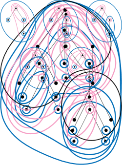
Figure 2. An upper tube and its corresponding lower tube. The type of the upper tube is the decoration of the highlighted edge.

To generalize the tubing expansion to this case, we need the appropriate generalizations of the statistics that appear in Theorem 2.8. Let $t$ be an $(I,\mathcal{E})$-tree and $\tau$ be a binary tubing of $t$. Suppose $t^{\prime}\in\tau$ is an upper tube and $t^{\prime\prime}$ the corresponding lower tube (i.e. the unique lower tube such that $t^{\prime}\cup t^{\prime\prime}\in\tau$). We define the type of $t^{\prime}$ to be the decoration of the first edge on the unique path from $\operatorname{rt}t^{\prime}$ to $\operatorname{rt}t^{\prime\prime}$. By construction, the type is an element of $E_{i}$ where $i=d(t^{\prime})$ is the decoration of the root vertex of $t^{\prime}$. Note we only assign types to upper tubes, not lower tubes. For each vertex $v\in t$ and edge type $e\in E_{d(v)}$ define the $e$-rank $\operatorname{rk}_{e}(\tau,v)$ to be the number of upper tubes of type $e$ rooted at $v$. Collect these together to get the rank vector $\operatorname{\mathbf{rk}}(\tau,v)\in\mathbb{Z}_{\geq 0}^{E_{d(v)}}$. Clearly $|\operatorname{\mathbf{rk}}(\tau,v)|=\operatorname{rk}(\tau,v)$. Then we define the Mellin monomial of $\tau$ to be

$$\operatorname{mel}(\tau)=\prod_{\begin{subarray}{c}v\in t\\ v\neq\operatorname{rt}t\end{subarray}}a_{d(v),\operatorname{\mathbf{rk}}(\tau,v)}.$$

The analogue of the $b$-statistic is slightly more complicated. For $1\leq k\leq b(\tau)$ write $\beta_{i}^{k}(\tau)$ the number of upper tubes of type $i$ containing (hence rooted at) $\operatorname{rt}t$, excluding the outermost $k-1$ upper tubes. Collect these into a vector $\beta^{k}(\tau)$ (which for lack of a better name we simply term the $k$th $\beta$-vector of $\tau$). Thus $\beta^{1}(\tau)=\operatorname{\mathbf{rk}}(\tau,\operatorname{rt}t)$ and $|\beta^{k}(\tau)|=b(\tau)-k$. We are now ready to state our expansion.

Theorem 3.6.

With the above setup, the unique map $\phi\colon\widetilde{\mathcal{H}}_{I,\mathcal{E}}\to\mathbb{K}[L]$ satisfying $\phi\tilde{B}_{+}^{(i)}=\Lambda_{i}\phi$ is given on trees by the formula

(36) $$\phi(t)=\sum_{\tau\in\mathrm{Tub}(t)}\operatorname{mel}(\tau)\sum_{k=1}^{b(\tau)}a_{d(t),\beta^{k}(\tau)}\frac{L^{k}}{k!}.$$

To prove this, we follow the structure of the argument as in Section 4 of [4], with some added complexity. We will temporarily write $\psi$ for the right side of 36. Let $\sigma$ be the linear term of $\psi$, i.e.

$$\sigma(t)=\sum_{\tau\in\mathrm{Tub}(t)}a_{d(t),\beta^{1}(\tau)}\operatorname{mel}(\tau).$$

and $\sigma$ vanishes on disconnected forests.

For any tree $t$ and $k\geq 1$,

$$\sigma^{*k}(t)=\sum_{\begin{subarray}{c}\tau\in\mathrm{Tub}(t)\\ b(\tau)\geq k\end{subarray}}a_{d(t),\beta^{k}(\tau)}\operatorname{mel}(\tau).$$

(Note that, $\sigma^{*k}$ can be nonzero on disconnected forests, but we are claiming this equality only for trees (see also the remark after Lemma 4.3 in [4]).)

Proof.

By induction on $k$. The base case is true by definition. Then

$$\sigma^{*k+1}(t)=\sum_{f\in J(t)}\sigma(f)\sigma^{*k}(t\setminus f)$$

but $\sigma$ is an infinitesimal character so $\sigma(f)\neq 0$ only if $f$ is actually a tree. Moreover, clearly $\sigma^{*k}(1)=0$, so we can restrict the sum to proper subtrees $t^{\prime}$. Then inductively we have

$$\sigma^{*k+1}(t) =\sum_{t^{\prime}}\sigma(t^{\prime})\sigma^{*k}(t\setminus t^{\prime})$$

$$=\sum_{t^{\prime}}\sum_{\tau^{\prime}\in\mathrm{Tub}(t^{\prime})}\sum_{\begin{subarray}{c}\tau^{\prime\prime}\in\mathrm{Tub}(t\setminus t^{\prime})\\ b(\tau^{\prime\prime})\geq k\end{subarray}}a_{d(t^{\prime}),\beta^{1}(\tau^{\prime})}\operatorname{mel}(\tau^{\prime})a_{d(t),\beta^{k}(\tau^{\prime\prime})}\operatorname{mel}(\tau^{\prime\prime}).$$

By the recursive construction of tubings (Section 2.6), $\tau^{\prime}$ and $\tau^{\prime\prime}$ uniquely determine a tubing $\tau\in\mathrm{Tub}(t)$. Note that for any vertex $v\in t^{\prime}$, the upper tubes of $\tau$ rooted at $v$ are the same as those of $\tau^{\prime}$, so $\operatorname{\mathbf{rk}}(\tau,v)=\operatorname{\mathbf{rk}}(\tau^{\prime},v)$. The same is true for vertices of $\tau^{\prime\prime}$ other than $\operatorname{rt}t$. Thus we have have

$$\operatorname{mel}(\tau)=\operatorname{mel}(\tau^{\prime})a_{d(t^{\prime}),\operatorname{\mathbf{rk}}(\tau,\operatorname{rt}t^{\prime})}\operatorname{mel}(\tau^{\prime\prime})=\operatorname{mel}(\tau^{\prime})a_{d(t^{\prime}),\beta^{1}(\tau^{\prime})}\operatorname{mel}(\tau^{\prime\prime}).$$

Moreover, since $\beta^{k}$ ignores the outermost the $k-1$ upper tubes containing $\operatorname{rt}t$ by definition, we have $\beta^{k+1}(\tau)=\beta^{k}(\tau^{\prime\prime})$. Finally, there is one additional tube in $\tau$ containing the root, so $b(\tau)=b(\tau^{\prime\prime})+1$. Hence the triple sum simplifies to

$$\sigma^{*k+1}(t)=\sum_{\begin{subarray}{c}\tau\in\mathrm{Tub}(t)\\ b(\tau)\geq k+1\end{subarray}}a_{d(t),\beta^{k+1}(\tau)}\operatorname{mel}(\tau)$$

as wanted. ∎

For notational convenience, for $\alpha\in\mathbb{Z}_{\geq 0}^{E_{i}}$ let us write $\sigma^{[\alpha]}$ for the linear form on $\mathcal{H}_{D,\mathcal{I}}^{\otimes I_{d}}$ given by

$$\sigma^{[\alpha]}=\bigotimes_{e\in E_{d}}\sigma^{*\alpha_{e}}.$$

Note that the coalgebra structure on $\mathcal{H}_{I,\mathcal{E}}^{\otimes E_{i}}$ gives a convolution product on linear forms; one easily checks that $\sigma^{[\alpha+\beta]}=\sigma^{[\alpha]}*\sigma^{[\beta]}$.

For $i\in I$,

$$\sigma\tilde{B}_{+}^{(i)}=\sum_{\alpha\in\mathbb{Z}_{\geq 0}^{E_{i}}}\binom{|\alpha|}{\alpha}a_{i,\alpha}\sigma^{[\alpha]}.$$

Proof.

For each $i\in I$ and $\alpha\in\mathbb{Z}_{\geq 0}^{E_{i}}$ let $\sigma_{i,\alpha}$ be the infinitesimal character defined by

$$\sigma_{i,\alpha}(t)=\begin{cases}\sum_{\tau\in\mathrm{Tub}(t),\beta^{1}(\tau)=\alpha}\operatorname{mel}(\tau)&d(t)=i\\ 0&\text{otherwise}\end{cases}$$

so that we have

$$\sigma=\sum_{i\in I}\sum_{\alpha\in\mathbb{Z}_{\geq 0}^{E_{i}}}a_{i,\alpha}\sigma_{i,\alpha}.$$

Note that we have $\sigma_{i,\alpha}\tilde{B}_{+}^{(j)}=0$ when $i\neq j$, so to get the desired formula it suffices to show that $\sigma_{i,\alpha}\tilde{B}_{+}^{(i)}=\binom{|\alpha|}{\alpha}\sigma^{[\alpha]}$ for $i\in I$ and $\alpha\in\mathbb{Z}_{\geq 0}^{E_{i}}$. We do this by induction on $m=|\alpha|$.

Now, for $\alpha=0$ we have that $\sigma_{i,\alpha}(t)=1$ if $t$ is the one-vertex tree with decoration $i$ and 0 otherwise. Of course $\sigma^{[0]}$ is 1 when each forest is empty and 0 otherwise, so we do indeed see that $\sigma_{i,0}\tilde{B}_{+}^{(i)}=\sigma^{[0]}$ as wanted.

Suppose now that $m>0$ and that the desired identity holds for smaller values. Then $\sigma_{i,\alpha}$ vanishes on one-vertex trees, so all tubings of interest have at least one upper tube. For $e\in E_{i}$, let $\sigma_{i,\alpha}^{e}(t)$ be the sum only for those tubings where the outermost upper tube has type $e$. Thus

$$\sigma_{i,\alpha}=\sum_{e\in E_{i}}\sigma_{i,\alpha}^{e}.$$

Note $\sigma^{e}_{i,\alpha}=0$ when $\alpha_{e}=0$, as in this case there must be no tube of type $i$ containing the root. Suppose now that $\alpha_{e}\neq 0$ and $t=\tilde{B}_{+}^{(i)}\left(\bigotimes_{e^{\prime}\in E_{i}}f_{e^{\prime}}\right)$. Let $\tau$ be a binary tubing of $t$ which recursively corresponds to $(\tau^{\prime},\tau^{\prime\prime})$. Then the outermost upper tube of $\tau$ is type $e$ precisely when the lower subtree $t^{\prime}$ is contained in $f_{e}$. Moreover in this case we have $\beta^{1}(\tau)=\beta^{1}(\tau^{\prime\prime})+1_{e}$, where $1_{e}$ is the indicator vector for $e$. Then we have

$$\sigma^{e}_{i,\alpha}(t)=\sum_{\begin{subarray}{c}t^{\prime}\subseteq f_{i}\\ \text{subtree}\end{subarray}}\sigma(t^{\prime})\sigma_{i,\alpha-1_{i}}(t\setminus t^{\prime}).$$

Now $t\setminus t^{\prime}=\tilde{B}_{+}^{(i)}\left(\bigotimes_{e^{\prime}}f^{\prime}_{e^{\prime}}\right)$ where $f^{\prime}_{e}=f_{e}\setminus t^{\prime}$ and $f^{\prime}_{e^{\prime}}=f_{e^{\prime}}$ for $e\neq e^{\prime}$. It follows that

$$\sigma^{e}_{i,\alpha}B_{+}^{(i)} =\sigma^{[1_{e}]}*\sigma_{i,\alpha-1_{e}}\tilde{B}_{+}^{(i)}$$

$$=\sigma^{[1_{e}]}*\binom{m-1}{\alpha-1_{e}}\sigma^{[\alpha-1_{e}]}$$

$$=\binom{m-1}{\alpha-1_{e}}\sigma^{[\alpha]}.$$

Finally, by summing over the values of $e$ we get

$$\sigma_{i,\alpha}\tilde{B}_{+}^{(i)}=\sum_{e\in E_{i}}\binom{m-1}{\alpha-1_{e}}\sigma^{[\alpha]}=\binom{m}{\alpha}\sigma^{[\alpha]}$$

by the multinomial analogue of the Pascal recurrence. ∎

Proof of Theorem 3.6.

Let $\Psi_{i}\colon\widetilde{\mathcal{H}}_{I,\mathcal{E}}^{\otimes E_{i}}\to\mathbb{K}[\mathbf{L}_{i}]$ be given by

$$\Psi_{i}\left(\bigotimes_{e\in E_{i}}f_{e}\right)=\prod_{e\in E_{i}}\left(\psi(f_{e})\big{|}_{L=L_{e}}\right).$$

This is simply the map $\psi^{\otimes E_{i}}$ carried through the identification of $\mathbb{K}[L]^{\otimes E_{i}}$ with $\mathbb{K}[\mathbf{L}_{i}]$. Thus, our goal is to show $\psi\tilde{B}_{+}^{(i)}=\Lambda_{i}\Psi_{i}$; by uniqueness this shows $\phi=\psi$. Note that since $\psi$ is an algebra morphism, we have

$$\Psi_{i}\left(\bigotimes_{e\in E_{i}}f_{e}\right)\bigg{|}_{L_{e}=L\,\forall e\in E_{i}}=\prod_{e\in E_{i}}\psi(f_{e})=\psi\left(\prod_{e\in E_{i}}f_{e}\right).$$

By Section 3.5 we have $\psi=\exp_{*}(L\sigma)$. Thus

$$\frac{d}{dL}\psi\tilde{B}_{+}^{(i)}=(\psi*\sigma)\tilde{B}_{+}^{(i)}=\psi*_{\delta}\sigma\tilde{B}_{+}^{(i)}$$

where $\delta$ is the coaction and the second equality is by Item 2.4(i). But observe that

$$\left(\psi*_{\delta}\sigma\tilde{B}_{+}^{(i)}\right)\left(\bigotimes_{e\in E_{i}}f_{e}\right) =\sum_{\begin{subarray}{c}f_{e}^{\prime}\in J(f_{e})\\ \forall e\in E_{i}\end{subarray}}\psi\left(\prod_{e\in E_{i}}f^{\prime}_{e}\right)\sigma\left(\tilde{B}_{+}^{(i)}\left(\bigotimes_{e\in e_{i}}(f_{e}\setminus f^{\prime}_{e})\right)\right)$$

$$=\sum_{\begin{subarray}{c}f_{e}^{\prime}\in J(f_{e})\\ \forall e\in E_{i}\end{subarray}}\Psi_{i}\left(\bigotimes_{e\in E_{i}}f^{\prime}_{e}\right)\sigma\left(\tilde{B}_{+}^{(i)}\left(\bigotimes_{e\in e_{i}}(f_{e}\setminus f^{\prime}_{e})\right)\right)\bigg{|}_{L_{e}=L\,\forall e\in E_{i}}$$

$$=\left(\Psi_{i}*\sigma\tilde{B}_{+}^{(i)}\right)\left(\bigotimes_{e\in E_{i}}f_{e}\right)\bigg{|}_{L_{e}=L\,\forall e\in E_{i}}.$$

Thus we have

$$\frac{d}{dL}\psi\tilde{B}_{+}^{(i)} =\Psi_{i}*\sigma\tilde{B}_{+}^{(i)}\big{|}_{L_{e}=L\,\forall e\in E_{i}}$$

$$=\left(\Psi_{i}*\sum_{\alpha\in\mathbb{Z}_{\geq 0}^{E_{i}}}\binom{|\alpha|}{\alpha}a_{i,\alpha}\sigma^{[\alpha]}\right)\bigg{|}_{L_{e}=L\,\forall e\in E_{i}}$$ by LABEL:thm:tubingtensor_lemma_2

$$=A_{i}(\partial/\partial L_{e}\colon e\in E_{i})\Psi\big{|}_{L_{e}=L\,\forall e\in E_{i}}$$

$$=\frac{d}{dL}\Lambda_{i}\Psi.$$

Since we also have

$$\psi(\tilde{B}_{+}^{(i)}1)=a_{i,0}=\Lambda_{i}(1)$$

this implies $\psi\tilde{B}_{+}^{(i)}=\Lambda_{i}\Psi_{i}$, as wanted. ∎

Finally, to solve 27 and 28, we need to lift them to combinatorial versions on the Hopf algebra $\widetilde{\mathcal{H}}_{P,\mathcal{E}}$ we introduced above, solve those, and then apply Theorem 3.6 to get a solution to the original equations. This time we will work in the full generality of systems from the start. The combinatorial version of the system 28 is

(37) $$T_{i}(x)=1+\sum_{p\in P_{i}}x^{w_{p}}\tilde{B}_{+}^{(p)}\left(\bigotimes_{e\in E_{p}}\mathbf{T}(x)^{\mu_{e}}\right).$$

As in Section 2.4, we are slightly abusing notation here by neglecting to notate the obvious (but non-injective) map $\widetilde{\mathcal{H}}_{P,\mathcal{E}}[[x]]^{\otimes E_{p}}\to\widetilde{\mathcal{H}}_{P,\mathcal{E}}^{\otimes E_{p}}[[x]]$. The formula generalizes that of Theorem 2.2. Each vertex will now have several outdegree vectors, one for each edge type: we write $\operatorname{od}_{i}(v,e)$ for the number of children of $v$ which have decorations lying in $P_{i}$ and such that the edge connecting them has decoration $e$. These are collected together into the outdegree vector $\operatorname{\mathbf{od}}(v,e)\in\mathbb{Z}_{\geq 0}^{I}$.

Theorem 3.7.

The unique solution to 37 is

$$T_{i}(x)=1+\sum_{t\in\mathcal{T}(P_{i})}\left(\prod_{v\in t}\prod_{e\in E_{d(v)}}\mu_{e}^{\underline{\operatorname{\mathbf{od}}(v,e)}}\right)\frac{tx^{w(t)}}{|\mathrm{Aut}(t)|}.$$

Proof.

Analogous to Theorem 2.1. ∎

As before, we can get a combinatorial expansion for the solution of the Dyson–Schwinger equation by applying our results on 1-cocycles.

Theorem 3.8.

The unique solution to 28 is

$$G_{i}(x,L)=1+\sum_{t\in\mathcal{T}(P_{i})}\left(\prod_{v\in t}\prod_{e\in E_{d(v)}}\mu_{e}^{\underline{\operatorname{\mathbf{od}}(v,e)}}\right)\sum_{\tau\in\mathrm{Tub}(t)}\operatorname{mel}(\tau)\sum_{k=1}^{b(\tau)}a_{d(t),\beta^{k}(\tau)}\frac{x^{w(t)}L^{k}}{|\mathrm{Aut}(t)|k!}.$$

Proof.

Immediate from Theorem 3.7 and Theorem 3.6. ∎

4. Conclusion

We have given a method to give combinatorially indexed and understandable series solutions to Dyson–Schwinger equations and systems thereof with distinguished insertion places. This concludes the single scale portion of the long-standing program one of us has to solve Dyson–Schwinger equations combinatorially. These solutions are powerful in that they give us combinatorial control over the expansions. So far this has resulted in physically interesting results on the leading log hierarchy [13, 12] and on resurgence [8], both of which would be interesting to investigate in the multiple insertion place case.

Paul Balduf has done some numerical computations of solutions to Dyson–Schwinger equations with two insertion places (see pp. 44, 45 of [3]). Interestingly, when the two insertion places degenerate into one by setting the power of one of the insertions (the parameter $s$) to $-1$, then the function does not appear to be differentiable based on the result of the numerical computation. It is not clear why this should be, and we certainly have no combinatorial understanding in this direction at present.

The program of solving Dyson–Schwinger equations with combinatorial expansions has also been interesting for pure combinatorics, first contributing to a renaissance in chord diagram combinatorics, and now suggesting connections to other notions of tubings in combinatorics, eg [10, 19], which deserve further investigation.

The main case of Dyson–Schwinger equation still outstanding is the case of non-single scale insertions as occurs in general vertex insertions. Non-single scale insertions can be addressed in the present framework by choosing one scale and then capturing the remaining kinematic dependence in dimensionless parameters, however this is inelegant in requiring a choice, and does not give any combinatorial or algebraic insight into the interplay of the different scales.

We have also used the Riordan group to more clearly explain the connection between Dyson–Schwinger equations and the renormalization group equation clarifying the known results in the single insertion case and generalizing to the multiple insertion place case. We proved and disproved conjectures of Nabergall [24].

References

- [1] Roland Bacher “Sur le groupe d’interpolation”, Preprint, 2006 arXiv:math/0609736 [math.CO]
- [2] Paul-Hermann Balduf “Dyson–Schwinger equations in minimal subtraction” Published online first In Annales de l’Institut Henri Poincaré, 2023 arXiv:2109.13684 [hep-th]
- [3] Paul-Hermann Balduf “Variations of single-kernel Dyson-Schwinger equations” https://paulbalduf.com/wp-content/uploads/2024/08/2024_08_Balduf_Bonn.pdf, Talk at ‘Combinatorics, Resurgence and Algebraic Geometry in Quantum Field Theory’, MPIM Bonn, August 23rd, 2024, 2024
- [4] Paul-Hermann Balduf, Amelia Cantwell, Kurusch Ebrahimi-Fard, Lukas Nabergall, Nicholas Olson-Harris and Karen Yeats “Tubings, chord diagrams, and Dyson–Schwinger equations” In Journal of the London Mathematical Society 110, 2024 URL: https://londmathsoc.onlinelibrary.wiley.com/doi/full/10.1112/jlms.70006
- [5] Marc P. Bellon “An Efficient Method for the Solution of Schwinger–Dyson equations for propagators” In Nuclear Physics B 826, 2010, pp. 522–531 arXiv:0907.2296 [hep-th]
- [6] Christoph Bergbauer and Dirk Kreimer “Hopf algebras in renormalization theory: locality and Dyson–Schwinger equations from Hochschild cohomology” In Physics and Number Theory, IRMA Lectures in Mathematics and Theoretical Physics 10 EMS Press, 2006, pp. 133–164 arXiv:hep-th/0506190
- [7] Michael Borinsky “Feynman graph generation and calculations in the Hopf algebra of Feynman graphs” In Computer Physics Communications 185, 2014, pp. 3317–3330 arXiv:1402.2613 [hep-th]
- [8] Michael Borinsky, Gerald V. Dunne and Karen Yeats “Tree-tubings and the combinatorics of resurgent Dyson-Schwinger equations”, Preprint, 2024 arXiv:2408.15883 [math-ph]
- [9] D.J. Broadhurst and D. Kreimer “Exact solutions of Dyson–Schwinger equations for iterated one-loop integrals and propagator-coupling duality” In Nuclear Physics B 600, 2001, pp. 403–422 arXiv:hep-th/0012146
- [10] Michael Carr and Satyan L. Devadoss “Coxeter complexes and graph-associahedra” In Topology and its Applications 153, 2006, pp. 2155–2168 arXiv:math/0407229 [math.QA]
- [11] Alain Connes and Dirk Kreimer “Hopf algebras, renormalization and noncommutative geometry” In Communications in Mathematical Physics 199, 1998, pp. 203–242 arXiv:hep-th/9808042
- [12] Julien Courtiel and Karen Yeats “Next-tok Leading Log Expansions by Chord Diagrams” In Communications in Mathematical Physics 377, 2020, pp. 469–501 arXiv:1906.05139 [math-ph]
- [13] Julien Courtiel and Karen Yeats “Terminal chords in connected chord diagrams” In Annales de l’Institut Henri Poincaré 4, 2017, pp. 417–452 arXiv:1603.08596 [math.CO]
- [14] Julien Courtiel, Karen Yeats and Noam Zeilberger “Connected Chord Diagrams and Bridgeless Maps” In Electronic Journal of Combinatorics 26, 2019 URL: https://www.combinatorics.org/ojs/index.php/eljc/article/view/v26i4p37
- [15] Yukio Doi “Homological coalgebra” In Journal of the Mathematical Society of Japan 33, 1981, pp. 31–50
- [16] William T. Dugan “Sequences of Trees and Higher-Order Renormalization Group Equations”, 2019 URL: https://uwspace.uwaterloo.ca/handle/10012/14957
- [17] Loïc Foissy “General Dyson–Schwinger equations and systems” In Communications in Mathematical Physics 327, 2014, pp. 151–179 arXiv:1112.2606 [math.RA]
- [18] Loïc Foissy “Multigraded Dyson-Schwinger systems” In Journal of Mathematical Physics 61, 2020, pp. 051703 arXiv:1511.06859 [math.RA]
- [19] Pavel Galashin “-associahedra” In Selecta Mathematica 30, New Series, 2023 arXiv:2110.07257 [math.CO]
- [20] Markus Hihn and Karen Yeats “Generalized chord diagram expansions of Dyson–Schwinger equations” In Annales de l’Institut Henri Poincaré 6, 2019, pp. 573–605 arXiv:1602.02550 [math-ph]
- [21] Donald Knuth “Searching and Sorting” Addison-Wesley, 1998
- [22] Dirk Kreimer “On Overlapping Divergences” In Communications in Mathematical Phyiscs 204, 1999, pp. 669–689 arXiv:q-alg/9707029
- [23] Nicolas Marie and Karen Yeats “A chord diagram expansion coming from some Dyson-Schwinger equations” In Communications in Number Theory and Physics 7, 2014, pp. 251–291 arXiv:1210.5457 [math.CO]
- [24] Lukas Nabergall “Enumerative perspectives on chord diagrams”, 2022 URL: https://uwspace.uwaterloo.ca/items/51239c85-b044-4e6b-97c6-710332c37c93
- [25] Nicholas Olson-Harris “Some Applications of Combinatorial Hopf Algebras to Integro-Differential Equations and Symmetric Function Identities”, 2024 URL: https://uwspace.uwaterloo.ca/items/8761e865-af96-42a1-8412-cd606585d152
- [26] Erik Panzer “Hopf-algebraic renormalization of Kreimer’s toy model”, 2011 arXiv:1202.3552 [math.QA]
- [27] David Prinz “Gauge Symmetries and Renormalization” In Mathematical Physics, Analysis and Geometry 25, 2022 arXiv:2001.00104 [hep-th]
- [28] Louis W. Shapiro, Seyoum Getu, Wen-Jin Woan and Leon C. Woodson “The Riordan group” In Discrete Applied Mathematics 34, 1991, pp. 229–239
- [29] Richard P. Stanley 2.62, Cambridge Studies in Advanced Mathematics Cambridge University Press, 1999
- [30] Walter D. Suijlekom “Renormalization of Gauge Fields using Hopf Algebras” In Quantum Field Theory Springer, 2009, pp. 135–154 arXiv:0801.3170 [math-ph]
- [31] Eric Swanson “A Primer on Functional Methods and the Schwinger-Dyson Equations” arXiv:1008.4337 In AIP Conference Proceedings 1296, 2010 DOI: 10.1063/1.3523221
- [32] Benjamin C. Ward “Massey products for graph homology” In International Mathematics Research Notices 2022, 2021, pp. 8086–8161 URL: https://academic.oup.com/imrn/article/2022/11/8086/6071864
- [33] Karen Yeats “A Combinatorial Perspective on Quantum Field Theory”, Springer Briefs in Mathematical Physics 15 Springer, 2017
- [34] Karen Yeats “Growth estimates for Dyson-Schwinger equations”, 2008