Deeply virtual $\phi$-meson production near threshold

Abstract

We discuss exclusive $\phi$-meson electroproduction off the proton near threshold within the GPD factorization framework. We propose the ‘threshold approximation’ in which only the leading term of the conformal partial wave expansion of the meson production amplitudes is kept in both the quark and gluon exchange channels. We test the validity of this approximation to next-to-leading order in QCD and demonstrate the strong sensitivity of the cross section to the gluon and strangeness gravitational form factors. We also perform realistic event generator simulations both for Jefferson Lab and EIC kinematics and demonstrate the capabilities of future facilities for measuring near-threshold $\phi$ electroproduction.

I Introduction

The exclusive production of the $\phi$-meson ($\phi(1020)$) in electron-proton scattering serves as a fascinating laboratory for studying the nucleon structure due to the unique status of the $\phi$ in QCD. In electroproduction mediated by a longitudinally polarized photon with high virtuality $Q^{2}\gg\Lambda_{\rm QCD}^{2}$, commonly called Deeply Virtual Meson Production (DVMP), a QCD factorization theorem Collins et al. (1997) allows for the first-principle treatment of the process in terms of the Generalized Parton Distributions (GPDs) Goloskokov and Kroll (2007); Čuić et al. (2023). In contrast to the production of lighter mesons, such as $\pi$, $\rho$, and $\omega$, $\phi$-production gives access to the gluon GPD even at low energy due to its flavor content $s\bar{s}$. Heavier quarkonium states such as $J/\psi$ (a $c\bar{c}$ bound state) and $\Upsilon$ (a $b\bar{b}$ bound state) are also sensitive to the gluon GPD, but their production typically requires additional theoretical tools such as non-relativistic QCD (NRQCD). $\phi$-production can be described by the usual light-cone distribution amplitude (DA), enjoys a higher production rate than $J/\psi$-production, and can be well-identified in experiments through the $KK$ decay channels. Measurements at different energies have been conducted at Cornell Dixon et al. (1979); Cassel et al. (1981), LEPS Mibe et al. (2005), HERA Adloff et al. (2000); Aaron et al. (2010); Chekanov et al. (2005), and Jefferson laboratory (JLab) Lukashin et al. (2001); Santoro et al. (2008); Seraydaryan et al. (2014); Dey et al. (2014).

One might argue that $\phi$-production is not ideally suited for probing the gluonic content of the proton because the process can be ‘contaminated’ by the intrinsic strangeness content. To what extent the latter contributes depends on experimental parameters as well as theoretical interpretations and is presently not well understood. However, one can reverse the argument and convert this feature into an additional advantage. That is, if one has enough knowledge about the gluon GPD from other processes such as $J/\psi$ production, $\phi$-production offers a unique opportunity to access the strangeness GPDs, which are otherwise very difficult to constrain.

In this paper, we study $\phi$-meson electroproduction near threshold and at high photon virtualities Hatta and Strikman (2021) in the GPD factorization framework. Our goal is to provide a benchmark calculation with next-to-leading order (NLO) perturbative QCD ingredients that can be readily used for the ongoing and proposed experimental projects at JLab and, in the long run, to motivate measurements of this process at the future Electron-Ion Collider (EIC) Abdul Khalek et al. (2022) at Brookhaven National Laboratory. Our study is complementary to the recent theoretical Hatta and Yang (2018); Hatta et al. (2019); Mamo and Zahed (2020); Wang et al. (2020); Du et al. (2020); Boussarie and Hatta (2020); Mamo and Zahed (2021); Guo et al. (2021); Kharzeev (2021); Sun et al. (2021, 2022); Winney et al. (2023); Guo et al. (2024) and experimental Ali et al. (2019); Duran et al. (2023); Adhikari et al. (2023) efforts to understand the near-threshold photoproduction of $J/\psi$. A major driving force of these developments is the recognition that this process is highly sensitive to the proton’s gravitational form factors (GFFs) Kobzarev and Okun (1962); Pagels (1966); Ji (1997)

$$\langle p^{\prime}|T_{q,g}^{\alpha\beta}|p\rangle = \bar{u}(p^{\prime})\left[A_{q,g}(t)\gamma^{(\alpha}P^{\beta)}+B_{q,g}(t)\frac{P^{(\alpha}i\sigma^{\beta)\lambda}\Delta_{\lambda}}{2M}+D_{q,g}(t)\frac{\Delta^{\alpha}\Delta^{\beta}-g^{\alpha\beta}\Delta^{2}}{4M}+\bar{C}_{q,g}(t)Mg^{\alpha\beta}\right]u(p),$$ (1)

where $T^{\alpha\beta}_{q,g}$ are the quark and gluon parts of the QCD energy momentum tensor ($A^{(\alpha}B^{\beta)}\equiv\frac{A^{\alpha}B^{\beta}+A^{\beta}B^{\alpha}}{2}$), $M$ is the proton mass, $P=\frac{p+p^{\prime}}{2}$, and $\Delta=p^{\prime}-p$. The connection between near-threshold production and the gluon GFFs $A_{g},~D_{g}$, and $\bar{C}_{g}$ was originally pointed out using an approach based on holographic QCD at strong coupling Hatta and Yang (2018); Hatta et al. (2019) where the energy momentum tensor plays a special role. Remarkably, the same is true also in GPD-based approaches at weak coupling Hatta and Strikman (2021); Guo et al. (2021) for a quite different reason. The first attempt to extract the gluon GFFs $A_{g}(t)$ and $D_{g}(t)$ has been recently made in Duran et al. (2023) by comparing the latest $J/\psi$ data at JLab with holographic QCD Mamo and Zahed (2021) and GPD Guo et al. (2021) calculations. However, the result is not without controversy, as the extraction relies on a single observable rather than a combination of multiple observables as is standard in QCD global analyses. Moreover, there are large theoretical uncertainties in the leading order (LO) perturbative QCD and holographic QCD calculations. As a matter of fact, the experimental data can be explained by other theoretical approaches without any reference to GFFs Du et al. (2020); Sun et al. (2021, 2022); Winney et al. (2023).

In order to make progress, one needs more observables with equally good or better sensitivities to the GFFs. There are a few possibilities. Instead of $J/\psi$, one can consider $\Upsilon$-production Hatta et al. (2019) where the large $\Upsilon$ mass (9.46 GeV) better justifies the use of peturbative QCD approaches. Alternatively, near-threshold electroproduction of $J/\psi$ Boussarie and Hatta (2020) may be an option, since the photon virtuality $Q^{2}$ can be adjusted well into the perturbative QCD domain. However, both of these alternatives, although worth pursuing, suffer from low production rates that pose experimental challenges even with the high luminosities at JLab and the EIC. Furthermore, $\Upsilon$ cannot be produced on proton targets at the current JLab energy.

Under these circumstances, $\phi$-meson electroproduction near threshold Hatta and Strikman (2021) emerges as a viable and attractive possibility. Due to the relatively low mass of the $\phi$-meson, the cross section is measurably large even for perturbative values of $Q^{2}$. Compared to $J/\psi$ photoproduction where the hard scale ($J/\psi$ mass) is fixed, a variable hard scale $Q$ provides an additional experimental parameter that can be adjusted for certain purposes. As we shall demonstrate, the cross section is strongly sensitive to the gluon and strangeness GFFs, in particular the strangeness D-term $D_{s}(t=0)$ which was the main focus of Hatta and Strikman (2021). The present work, albeit restricted to the longitudinal cross section, provides a proper QCD-based prediction that should supersede the heuristic discussion in Hatta and Strikman (2021).

In addition to enhancing the theoretical framework, we will conduct a feasibility study for experimental measurements at future facilities by integrating the updated theoretical predictions into the lAger Joosten (2021) event generator. The EIC offers the necessary flexibility and luminosity to perform the first measurements of near-threshold meson production at an $e+p$ collider. At Jefferson Lab, the Solenoidal Large Intensity Device (SoLID) provides an excellent platform for utilizing near-threshold $\phi$ and $J/\psi$ electroproduction to study gravitational form factors due to its large acceptance and high instantaneous luminosity.

II Kinematics

The process of interest is the exclusive production of the $\phi$-meson in unpolarized electron-proton scattering $ep\to e^{\prime}\gamma^{*}p\to e^{\prime}p^{\prime}\phi$. At fixed $ep$ center-of-mass energy $s_{ep}=(l+p)^{2}$, the cross section integrated over azimuthal angles is characterized by the photon virtuality $q^{2}=-Q^{2}$, the Bjorken variable $x_{B}=\frac{Q^{2}}{2p\cdot q}$ and the proton momentum transfer $t=(p^{\prime}-p)^{2}$. The standard inelasticity parameter $y$ in deeply inelastic scattering (DIS) can be written in terms of these variables:

$$y=\frac{q\cdot p}{l\cdot p}=\frac{Q^{2}}{s_{ep}x_{B}}.$$ (2)

For the present purpose, it is convenient to introduce the $\gamma^{*}p$ center-of mass-energy

$$W^{2}=(p+q)^{2}=M^{2}-Q^{2}+2p\cdot q=M^{2}+Q^{2}\frac{1-x_{B}}{x_{B}},$$ (3)

to be used interchangeably with $x_{B}$ and work in the $\gamma^{*}p$ center-of-mass frame. In this frame, one can parameterize the momenta in the reaction $\gamma^{*}(q)+p\to\phi(k)+p^{\prime}$ as

$$p^{\mu}=(E_{cm},0,0,p_{cm})=\left(\frac{W^{2}+Q^{2}+M^{2}}{2W},0,0,p_{cm}\right),$$

$$q^{\mu}=(\sqrt{p_{cm}^{2}-Q^{2}},0,0,-p_{cm})=\left(\frac{W^{2}-M^{2}-Q^{2}}{2W},0,0,-p_{cm}\right),$$

$$p^{\prime\mu}=(E^{\prime}_{cm},\vec{k}_{cm})=\left(\frac{W^{2}-M_{\phi}^{2}+M^{2}}{2W},\vec{k}_{cm}\right),$$

$$k^{\mu}=(\sqrt{M_{\phi}^{2}+k_{cm}^{2}},-\vec{k}_{cm})=\left(\frac{W^{2}+M_{\phi}^{2}-M^{2}}{2W},-\vec{k}_{cm}\right),$$ (4)

where $E_{cm}=\sqrt{M^{2}+p_{cm}^{2}}$, $E^{\prime}_{cm}=\sqrt{M^{2}+k_{cm}^{2}}$, and

$$p_{cm}^{2} = \frac{W^{4}-2W^{2}(M^{2}-Q^{2})+(M^{2}+Q^{2})^{2}}{4W^{2}},$$

$$k_{cm}^{2} = \frac{(W^{2}-(M_{\phi}+M)^{2})(W^{2}-(M_{\phi}-M)^{2})}{4W^{2}}.$$ (5)

For a fixed value of $W$, the momentum transfer

$$-t = -\left(\sqrt{p_{cm}^{2}+M^{2}}-\sqrt{k_{cm}^{2}+M^{2}}\right)^{2}+(\vec{p}_{cm}-\vec{k}_{cm})^{2}$$ (6)

$$= -\left(\frac{Q^{2}+M_{\phi}^{2}}{2W}\right)^{2}+p_{cm}^{2}+k_{cm}^{2}-2p_{cm}k_{cm}\cos\theta,$$

varies in the window

$$-t_{min}<-t<-t_{max},$$ (7)

where

$$-t_{min}=-\left(\frac{Q^{2}+M_{\phi}^{2}}{2W}\right)^{2}+(p_{cm}-k_{cm})^{2},$$

$$-t_{max}=-\left(\frac{Q^{2}+M_{\phi}^{2}}{2W}\right)^{2}+(p_{cm}+k_{cm})^{2}.$$ (8)

The range (7) is plotted in Fig. 1 for $Q^{2}=6$ GeV² (left) and $Q^{2}=10$ GeV² (right) above the threshold energy

$$W\geq W_{th}\equiv M_{\phi}+M=1.02\,{\rm GeV}+0.94\,{\rm GeV}=1.96\,{\rm GeV}.$$ (9)

Fig. 1 also shows contours of the skewness variable ($p^{+}\equiv\frac{1}{\sqrt{2}}(p^{0}+p^{3})$)

$$\xi=\frac{p^{+}-p^{\prime+}}{p^{+}+p^{\prime+}} = \frac{\sqrt{M^{2}+p_{cm}^{2}}+p_{cm}-\sqrt{M^{2}+k_{cm}^{2}}-k_{cm}\cos\theta}{\sqrt{M^{2}+p_{cm}^{2}}+p_{cm}+\sqrt{M^{2}+k_{cm}^{2}}+k_{cm}\cos\theta}$$ (10)

$$= \frac{2(p_{cm}+E_{cm})(E_{cm}-E^{\prime}_{cm})-t}{2(p_{cm}+E_{cm})(E_{cm}+E^{\prime}_{cm})-4M^{2}+t},$$

which will be an important parameter in this work. There exist various definitions of the skewness variable, but these differences vanish in the limit $Q\rightarrow\infty$. Our definition is tied to the $\gamma^{*}p$ center-of-mass frame. With this choice, $t_{min}$ is related to $\xi$ as

$$t_{min}=-\frac{4\xi^{2}M^{2}}{1-\xi^{2}},$$ (11)

which represents the intersection point between a curve of constant $\xi$ and the $t_{min}$ curve in Fig. 1.

\begin{overpic}[width=433.62pt]{6.pdf} \put(-6.0,50.0){\rotatebox{90.0}{\small$|t|\ (\mathrm{GeV}^{2})$}} \par\put(10.0,85.0){{\color[rgb]{0,0,0}\raisebox{2.15277pt}{\rule{20.00003pt}{1.0pt}}} Isolines of constant $\xi$} \par\put(45.0,-5.0){\small$W\ (\mathrm{GeV})$} \end{overpic}

\begin{overpic}[width=433.62pt]{10.pdf} \put(-6.0,50.0){\rotatebox{90.0}{\small$|t|\ (\mathrm{GeV}^{2})$}} \put(10.0,85.0){{\color[rgb]{0,0,0}\raisebox{2.15277pt}{\rule{20.00003pt}{1.0pt}}} Isolines of constant $\xi$} \put(45.0,-5.0){\small$W\ (\mathrm{GeV})$} \end{overpic}

Figure 1: Contour plots of $\xi$ in the $(W,|t|)$ plane at $Q^{2}=6$ GeV² (left) and $Q^{2}=10$ GeV² (right). The horizontal line is at $|t|=\frac{Q^{2}}{3}$.

The differential cross section takes the form

$$\frac{d\sigma}{dWdQ^{2}dt} = \frac{\alpha_{em}}{4\pi}\frac{W(W^{2}-M^{2})}{(p\cdot l)^{2}Q^{2}(1-\varepsilon)}\frac{d\sigma^{\gamma^{*}p}}{dt},$$ (12)

where

$$\varepsilon=\frac{1-y-\frac{y^{2}\gamma^{2}}{4}}{1-y+\frac{y^{2}}{2}+\frac{y^{2}\gamma^{2}}{4}}$$ (13)

is the ratio of the longitudinal and transverse photon fluxes (see below) and $\gamma=\frac{2x_{B}M}{Q}$ is a parameter characterizing target mass corrections which is actually not negligible in the present kinematics. $\frac{d\sigma^{\gamma^{*}p}}{dt}$ is the differential cross section in the $\gamma^{*}p$ subsystem. It consists of the transverse and longitudinal parts

$$\frac{d\sigma^{\gamma^{*}p}}{dt} = \frac{\alpha_{em}}{8(W^{2}-M^{2})Wp_{cm}}\left(\frac{1}{2}g_{\perp}^{\mu\nu}+\varepsilon\epsilon_{L}^{\mu}\epsilon_{L}^{\nu}\right)\frac{1}{2}\sum_{spin}\langle p|J^{em}_{\mu}(-q)|p^{\prime}\phi\rangle\langle p^{\prime}\phi|J^{em}_{\nu}(q)|p\rangle$$ (14)

$$= \frac{d\sigma_{T}}{dt}+\varepsilon\frac{d\sigma_{L}}{dt},$$

where $g_{\perp}^{ij}=-\delta^{ij}$ ($i,j=1,2$) and $\epsilon_{L}^{\mu}$ is the longitudinal photon polarization vector. The following formula may be useful to connect seemingly different expressions in the literature:

$$\frac{x_{B}^{2}}{Q^{4}(1-x_{B})\sqrt{1+\gamma^{2}}}=\frac{1}{2(W^{2}-M^{2})Wp_{cm}}.$$ (15)

Experimentally, it is straightforward to measure the differential (14) and integrated cross sections

$$\sigma^{\gamma^{*}p}=\int^{t_{max}}_{t_{min}}dt\frac{d\sigma^{\gamma^{*}p}}{dt}=\sigma_{T}(W,Q)+\varepsilon\sigma_{L}(W,Q)=\left(\frac{1}{R(W,Q)}+\varepsilon\right)\sigma_{L}(W,Q),$$ (16)

where the ratio

$$R(W,Q)=\frac{\sigma_{L}}{\sigma_{T}}$$ (17)

is commonly introduced in the literature. In principle, it is possible to experimentally measure $R(W,Q)$ by monitoring the $\varepsilon$-dependence (equivalently, the energy $s_{ep}$ dependence) or measuring the decay products of $\phi$. We shall comment more on this in a later section.

At HERA, exclusive $\phi$-production has been measured at high energy, up to $W\sim 130$ GeV and $Q^{2}\lesssim 40$ GeV² Adloff et al. (2000); Chekanov et al. (2005); Aaron et al. (2010), primarily motivated by the physics of diffraction at $x_{B}\ll 1$. Such vector meson electroproduction data have been utilized for modeling GPDs at LO Goloskokov and Kroll (2007); Meskauskas and Müller (2014) and, more recently, as inputs for global analyses of GPDs at NLO in deeply virtual Compton scattering (DVCS) and DVMP Lautenschlager et al. (2013); Čuić et al. (2023). Turning to the low energy side, the LEPS collaboration Mibe et al. (2005) has measured the photoproduction ($Q=0$) cross section near the threshold $W_{th}\leq W\leq 2.31$ GeV ($1.57\leq E_{\gamma}\leq 2.37\,{\rm GeV}$ in terms of the photon energy in the target (proton) rest frame). Subsequently, the CLAS collaboration Santoro et al. (2008) has measured the electroproduction cross section in the range $W_{th}<W<3$ GeV and $1.4<Q^{2}<3.8$ GeV². Currently, there are several experimental proposals at JLab to measure electroproduction near the threshold at higher $Q^{2}$, and the effort can be continued in the future with the EIC.

III GPD factorization

III.1 General consideration

The goal of this paper is to provide predictions for the longitudinal differential $\frac{d\sigma_{L}}{dt}$ and total $\sigma_{L}$ cross sections near the threshold and at high values of $Q^{2}$. By near-threshold, we mean the energy region explored by the CLAS collaboration

$$W_{th}<W<3\,{\rm GeV}.$$ (18)

Practical reasons for this choice will be explained later. On the other hand, since our approach will be based on the QCD factorization framework treating $Q^{2}$ as a hard scale, we consider $Q^{2}$ values larger than those explored previously by the CLAS collaboration. Roughly, we have in mind $Q\gtrsim 2$ GeV. The exact value of $Q$ above which the perturbative description becomes valid cannot be sharply determined, but we will make a phenomenological estimate in the numerical section.

Let us first discuss practical and conceptual issues with the use of QCD factorization in the threshold region. First, as is clear from (3), when $Q^{2}$ is large the condition $W\gtrsim W_{th}$ is realized by a large cancellation between $Q^{2}$ and $2p\cdot q$. This means that the Bjorken variable is close to unity

$$x_{B}=\frac{Q^{2}}{2p\cdot q}\approx 1,$$ (19)

so the skewness variable is also close to unity

$$\xi\approx\frac{x_{B}}{2-x_{B}}\approx 1.$$ (20)

As a matter of fact, GPDs at large $\xi\sim{\cal O}(1)$ are poorly constrained. Existing global analyses heavily rely on HERA data which were mostly taken at $x_{B},\xi\ll 1$ (see Kumericki et al. (2016); Favart et al. (2016); Čuić et al. (2023) and references therein). Therefore, GPD models constrained at $\xi\ll 1$ need to be extrapolated to the region $\xi\sim{\cal O}(1)$, and there is no reliable way to do so. Moreover, when $\xi\ll 1$ where $t$ is also small, the helicity-flip $E$-type GPDs are often neglected since they typically enter cross sections with prefactors $\xi^{2}$ and $t/M^{2}$ (see for example (26) below). Near the threshold where $\xi\sim{\cal O}(1)$, their contributions are no longer negligible, but they are less well known compared to the $H$-type GPDs Kroll et al. (2013). Remarkably, however, in this regime, DVMP scattering amplitudes are largely insensitive to the $x$-dependence of GPDs. Instead they are dominated by the gravitational form factors (1) which are much easier to parameterize and evolve. This is actually the main point of this paper, and we will explain it in detail in the next subsections.

Another issue is that the momentum transfer $|t|$ tends to be large in the threshold region at high-$Q^{2}$, often much larger than $\Lambda_{\rm QCD}^{2}$, see Fig. 1. At the threshold,

$$|t_{th}|=\frac{M(M_{\phi}^{2}+Q^{2})}{M+M_{\phi}}\approx\frac{Q^{2}}{2}.$$ (21)

Above the threshold, $|t|$ varies in the window (7). It is easy to check that, in the kinematical region we consider ($Q>2$ GeV and $W<3$ GeV), $|t_{min}|$ grows linearly with $Q^{2}$. This is worrisome because higher twist corrections in GPD factorization formulas are of order $t/Q^{2}$. We can alleviate this problem by avoiding regions too close to the threshold and staying around $t\approx t_{min}$, see Fig. 1. However, experiments can in principle measure $\frac{d\sigma}{dt}$ in the entire range of $t$, and larger $t$-values are interesting since $\xi$ is also larger. As a compromise, we consider

$$|t_{min}|<|t|\lesssim\frac{Q^{2}}{3\,{\rm or}\,4}$$ (22)

to be the limit of applicability for our calculation. This limit is indicated by a horizontal line in Fig. 1. Above this line, higher twist corrections could be very large.

Finally, near the threshold, the relative velocity between the produced $\phi$ and the recoiling proton is small and can be nonrelativistic (zero at the threshold by definition). This means that there could be final state interactions (FSIs) which potentially break factorization Hatta and Strikman (2021). From a perturbative QCD perspective, the standard collinear factorization theorem Collins et al. (1997) assumes that the outgoing proton with momentum is collinear to the incoming proton

$$p^{\prime+}\gg p_{\perp}^{\prime}\gg p^{\prime-}.$$ (23)

This condition becomes increasingly difficult to satisfy as $\xi\to 1$ since $p^{\prime+}\propto 1-\xi$. Again one can circumvent this problem by avoiding the region too close to the threshold (see also a discussion in the $J/\psi$ case in Guo et al. (2021)). In the $\gamma^{*}p$ center-of-mass frame (4), the relative momentum in the final state is

$$(2k_{cm})^{2}\approx W^{2}-W^{2}_{th}\approx\left(\frac{1}{x_{B}}-1\right)Q^{2}\approx\frac{1-\xi}{2\xi}Q^{2}\equiv\mu_{th}^{2}.$$ (24)

The requirement of a large relative velocity can be expressed in a Lorentz-invariant manner by the condition that the ‘threshold scale’ $\mu_{th}^{2}$ should be much larger than the small scales

$$\frac{1-\xi}{2\xi}Q^{2}\gg|t|,M^{2}.$$ (25)

As soon as $\xi\gtrsim 1/3$, this becomes a stronger constraint than $Q^{2}\gg|t|$ and further shrinks the region of applicability toward $t\sim t_{min}$ and $\xi\lesssim 0.6$. However, whether this effect is numerically important in practice is largely unknown. Ultimately, what matters is the interaction strength between the produced meson and the recoiling proton, which depends on the meson species. In this regard, we refer to a recent dedicated study Kim et al. (2024) where it has been concluded that, near the threshold, the $\phi+p$ FSI cross section is orders of magnitude smaller than the production cross section. While Ref. Kim et al. (2024) concerns photoproduction, we expect the same conclusion holds in electroproduction since the final state is the same. We therefore neglect final-state interactions and stick to (22), although more investigations are certainly desirable.

III.2 Conformal partial wave expansion

For light vector meson production, QCD factorization has been proven only for the longitudinally polarized virtual photon Collins et al. (1997). We thus focus on the longitudinal cross section $\sigma_{L}$ in this section. The transverse cross section $\sigma_{T}$ will be phenomenologically included in a later section. Up to higher twist corrections of order $t/Q^{2}$, the differential cross section in (14) can be written as

$$\frac{d\sigma_{L}}{dt}=\frac{2\pi^{2}\alpha_{em}}{(W^{2}-M^{2})Wp_{cm}}\left((1-\xi^{2})|{\cal H}|^{2}-\left(\frac{t}{4M^{2}}+\xi^{2}\right)|{\cal E}|^{2}-2\xi^{2}{\rm Re}({\cal H}{\cal E}^{*})\right),$$ (26)

where ${\cal H}$ and ${\cal E}$ are the DVMP amplitudes which contain the GPDs $H^{q,g}$ and $E^{q,g}$, respectively. $q$ is the label for quark flavors. Throughout this paper, we consider four active flavors $n_{f}=4$, or $q=u,d,s,c$. ${\cal H}$ and ${\cal E}$ have the following factorized structure

$$\begin{pmatrix}{\cal H}(\xi,t,Q^{2})\\ {\cal E}(\xi,t,Q^{2})\end{pmatrix}=e_{s}\frac{C_{F}f_{\phi}}{N_{c}Q}\sum_{a=q,g}\begin{pmatrix}H^{a}(x,\xi,t,\mu^{2})\\ E^{a}(x,\xi,t,\mu^{2})\end{pmatrix}\otimes T^{a}\left(x,\xi,u,\frac{Q^{2}}{\mu^{2}}\right)\otimes\varphi(u,\mu^{2}),$$ (27)

where $e_{s}=-\frac{1}{3}$ is the electric charge (in units of $|e|$) of the $s$-quark. The notations $N_{c}=3$, $C_{F}=\frac{N_{c}^{2}-1}{2N_{c}}=\frac{4}{3}$ are standard. $\varphi(u)$ and $f_{\phi}$ are the $\phi$-meson distribution amplitude (DA) and the decay constant, respectively. $T^{a}$ are the hard scattering amplitudes, also referred to as coefficient functions. The symbols $\otimes$ represent convolutions in $-1<x<1$ and $0<u<1$. For simplicity, we have chosen the factorization scales of GPD and DA to be the same and equal to the renormalization scale $\mu^{2}$.

A particularly powerful framework to analyze the amplitude (27) is the conformal partial wave (CPaW) formalism developed in Mueller and Schafer (2006) and systematized to NLO in Kumericki et al. (2008) for DVCS and in Müller et al. (2014); Duplančić et al. (2017) for DVMP. It combines the conformal partial wave expansion in terms of the Gegenbauer polynomials with the Mellin-Barnes integral technique. Compared to the traditional momentum fraction representation, the CPaW formalism simplifies GPD evolution to NLO and beyond, enables innovative GPD modeling, and facilitates efficient code development for handling GPD evolution and data fitting. While the formalism is applicable to all kinematical regions, so far it has mostly been used in the small-$x_{B}$ region due to data availability (Čuić et al. (2023) and references therein). We argue here that, when applied to the threshold region of DVMP (large-$x_{B}$ and large-$\xi$), the CPaW formalism can be reduced to a very simple effective model which captures the physics of the QCD energy momentum tensor and GFFs Boussarie and Hatta (2020); Hatta and Strikman (2021); Guo et al. (2021, 2024), while retaining the connection to QCD factorization.

We first introduce the conformal moments for the meson DA

$$\varphi_{k}(\mu^{2})=\frac{2(2k+3)}{3(k+1)(k+2)}\int_{0}^{1}duC_{k}^{3/2}(2u-1)\varphi(u,\mu^{2}),\qquad(k:{\rm even})$$ (28)

where $C_{k}^{3/2}$ is the Gegenbauer polynomial. The inverse transform is

$$\varphi(u)=6u(1-u)\sum_{k=0}^{\rm even}\varphi_{k}C_{k}^{3/2}(2u-1).$$ (29)

As for the quark and gluon GPDs, we define

$$H^{q}_{j}(\xi,t)=\frac{\Gamma(3/2)\Gamma(j+1)}{2^{j}\Gamma(j+3/2)}\frac{1}{2}\int_{-1}^{1}dx\xi^{j}C_{j}^{3/2}(x/\xi)H^{q(+)}(x,\xi,t),\qquad(j:{\rm odd})$$ (30)

$$H^{g}_{j}(\xi,t)=\frac{\Gamma(3/2)\Gamma(j+1)}{2^{j}\Gamma(j+3/2)}\frac{1}{2}\int_{-1}^{1}dx\frac{3}{j}\xi^{j-1}C_{j-1}^{5/2}(x/\xi)H^{g}(x,\xi,t),\qquad(j:{\rm odd})$$ (31)

and similarly for $E_{j}^{q,g}(\xi,t)$. The notation $H^{q(+)}(x,\xi,t)=H^{q}(x,\xi,t)-H^{q}(-x,\xi,t)$ denotes the C-even part. The gluon GPD is normalized such that, in the forward limit, $H^{g}(x,0,0)=xG(x)$, where $G(x)$ is the unpolarized gluon PDF. These moments reduce to the standard Mellin moments of PDFs in the $\xi\to 0$ limit. The first moments $j=1$ are the quark and gluon GFFs (1)

$$H_{1}^{q,g}(\xi,t,\mu^{2})=A_{q,g}(t,\mu^{2})+\xi^{2}D_{q,g}(t,\mu^{2}),$$

$$E_{1}^{q,g}(\xi,t,\mu^{2})=B_{q,g}(t,\mu^{2})-\xi^{2}D_{q,g}(t,\mu^{2}).$$ (32)

In the moment space, the amplitudes (27) take the form

$$\begin{pmatrix}{\cal H}(\xi,t,Q^{2})\\ {\cal E}(\xi,t,Q^{2})\end{pmatrix}=\kappa\sum_{j=1}^{\rm odd}\sum_{k=0}^{\rm even}\sum_{a}\frac{2}{\xi^{j+1}}\begin{pmatrix}H_{j}^{a}(\xi,t,\mu^{2})\\ E_{j}^{a}(\xi,t,\mu^{2})\end{pmatrix}T^{a}_{jk}(Q^{2}/\mu^{2})\varphi_{k}(\mu^{2}),\qquad\kappa\equiv e_{s}\frac{C_{F}f_{\phi}}{N_{c}Q}.$$ (33)

Throughout this paper, we keep only the $k=0$ term for which $\varphi_{0}=1$. This is tantamount to assuming the asymptotic $\mu^{2}\to\infty$ formula for the DA $\varphi(u)\approx 6u(1-u)$. While the validity of this approximation is not fully understood, it is usually considered permissible and widely used in practice. If necessary, higher-$k$ terms Hua et al. (2021); Hu et al. (2024) can be included.

III.3 Threshold approximation

We now come to the crucial step of this work. We implement the ‘threshold approximation’ by keeping only the $j=1$ term in the sum (33)

$$\begin{pmatrix}{\cal H}(\xi,t,Q^{2})\\ {\cal E}(\xi,t,Q^{2})\end{pmatrix}\approx\frac{2\kappa}{\xi^{2}}\sum_{a}\begin{pmatrix}H_{1}^{a}(\xi,t,\mu^{2})\\ E_{1}^{a}(\xi,t,\mu^{2})\end{pmatrix}T^{a}_{10}(Q^{2}/\mu^{2}).$$ (34)

In contrast to the $k=0$ truncation, the $j=1$ truncation (34) is unusual and certainly does not hold in general. DVMP amplitudes are complex, and the imaginary part can only be recovered by performing the analytic continuation of the infinite sum (33) in the Mellin-Barnes representation Mueller and Schafer (2006); Müller et al. (2015). By keeping only the $j=1$ moment, one neglects the imaginary part from the beginning. However, scattering amplitudes near threshold are indeed dominantly real since there is no extra particle production by definition. In fact, (34) is known to be a good approximation when $\xi\approx 1$ in the gluon sector $a=g$ at least to leading order (LO) in perturbation theory. In other words, DVMP amplitudes in the gluon channel can be characterized by the gluon GFFs (32). This phenomenon has been first pointed out in Hatta and Strikman (2021); Guo et al. (2021) in the context of near-threshold $J/\psi$ production using the Mellin moment expansion of the scattering amplitude. Subsequently, it has been noticed in Guo et al. (2024) that the approximation is even better if one uses the conformal moment expansion.

On the other hand, in the quark channel $a=q$ relevant to the production of light mesons (including $\phi$), keeping only the first term of the Mellin moment expansion is not as good of an approximation as in the gluon channel Hatta and Strikman (2021). In the next subsection we demonstrate that, if one switches to the conformal moment expansion, the threshold approximation (34) is actually quite decent even in the quark sector. Furthermore, for the first time, we test the validity of the threshold approximation to next-to-leading order (NLO) in both the quark and gluon channels.

For this purpose, let us first write down (34) explicitly. The NLO hard coefficients $T_{jk}$ for DVMP are available in the literature Müller et al. (2014); Duplančić et al. (2017); Čuić et al. (2023). Keeping only the $T_{10}$ component and adjusting the flavor content to $\phi$-production, we find

$${\cal H}(\xi,t,Q^{2}) \approx \frac{2\kappa}{\xi^{2}}\frac{15}{2}\Biggl{[}\left\{\alpha_{s}(\mu)+\frac{\alpha_{s}^{2}(\mu)}{2\pi}\left(25.7309-2n_{f}+\left(-\frac{131}{18}+\frac{n_{f}}{3}\right)\ln\frac{Q^{2}}{\mu^{2}}\right)\right\}(A_{s}(t,\mu)+\xi^{2}D_{s}(t,\mu))$$

$$\qquad+\frac{\alpha_{s}^{2}}{2\pi}\left(-2.3889+\frac{2}{3}\ln\frac{Q^{2}}{\mu^{2}}\right)\sum_{q}(A_{q}+\xi^{2}D_{q})+\frac{3}{8}\left\{\alpha_{s}+\frac{\alpha_{s}^{2}}{2\pi}\left(13.8682-\frac{83}{18}\ln\frac{Q^{2}}{\mu^{2}}\right)\right\}(A_{g}+\xi^{2}D_{g})\Biggr{]},$$

$${\cal E}(\xi,t,Q^{2}) \approx \frac{2\kappa}{\xi^{2}}\frac{15}{2}\Biggl{[}\left\{\alpha_{s}(\mu)+\frac{\alpha_{s}^{2}(\mu)}{2\pi}\left(25.7309-2n_{f}+\left(-\frac{131}{18}+\frac{n_{f}}{3}\right)\ln\frac{Q^{2}}{\mu^{2}}\right)\right\}(B_{s}(t,\mu)-\xi^{2}D_{s}(t,\mu))$$

$$\qquad+\frac{\alpha_{s}^{2}}{2\pi}\left(-2.3889+\frac{2}{3}\ln\frac{Q^{2}}{\mu^{2}}\right)\sum_{q}(B_{q}-\xi^{2}D_{q})+\frac{3}{8}\left\{\alpha_{s}+\frac{\alpha_{s}^{2}}{2\pi}\left(13.8682-\frac{83}{18}\ln\frac{Q^{2}}{\mu^{2}}\right)\right\}(B_{g}-\xi^{2}D_{g})\Biggr{]}.$$

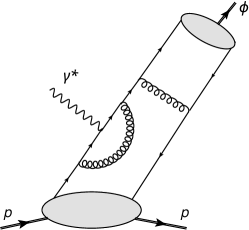
Figure 2: Representative NLO diagrams for the three terms in (III.3) and (III.3). Left: $s$-quark exchange. Middle: ‘pure singlet’ exchange. Right: gluon exchange.

The three contributions are depicted in Fig. 2. One can roughly estimate the size of each contribution using the following rule of thumb:

$$A_{u+d}\sim A_{g}\sim 10A_{s},\qquad\frac{\alpha_{s}}{\pi}\sim 0.1,$$ (37)

deferring the detailed numerical analysis to the next section. If we compare only the $A_{q,g}$ terms and assume a similar $t$-dependence for the quark and gluon GFFs, clearly the gluon exchange dominates in ${\cal H}$. The NLO correction for this term ${\cal O}(\alpha_{s}^{2})$ is sizable, about 60-70% of the leading order result. We also notice that the contribution from the $s$-quark exchange is comparable to that from $u,d$-quarks despite $A_{s}\ll A_{u+d}$ because the latter only enters at NLO. The relative minus sign suggests a significant cancellation between the two contributions. However, the inclusion of the $D_{q,g}$ terms may drastically change this expectation. Since $\xi^{2}\sim{\cal O}(1)$ and $D_{q,g}$ are supposedly negative, there can be a significant cancellation in $A_{q,g}+\xi^{2}D_{q,g}$ if $D_{q,g}$ are order unity. However, this cancellation may not be effective in the $s$-quark sector because $A_{s}\ll 1$. Therefore, if $D_{s}\sim{\cal O}(1)$, the $s$-quark contribution could become dominant Hatta and Strikman (2021). $D_{q,g}$ play an even more important role in ${\cal E}$ since there are indications that $B_{q,g}$ are very small Teryaev (1999); Hagler et al. (2008). As is clear from (26), when $\xi\sim{\cal O}(1)$, the ${\cal E}$ term is no longer negligible relative to the ${\cal H}$ term.

III.4 Accuracy of the threshold approximation

Let us investigate for which values of $\xi$ the threshold approximation (III.3), (III.3) can be a decent approximation to the full DVMP amplitude. We shall focus on the GPD $H$ and the associated amplitude ${\cal H}$, but the discussion for $E$ and ${\cal E}$ is entirely analogous. In the asymptotic limit $\mu^{2}\to\infty$ (corresponding to $Q^{2}\to\infty$) where $H_{g}(x,\xi)\propto\theta(\xi-|x|)(1-\frac{x^{2}}{\xi^{2}})^{2}$, the $j=1$ conformal moment by definition accounts for 100% of the LO amplitude, irrespective of the value of $\xi$. (In the Mellin moment expansion, the $j=1$ moment accounts for 80% of the amplitude in the limit $\xi\to 1$ Hatta and Strikman (2021); Guo et al. (2021).) If $\mu^{2}$ is finite this is not the case, however. Indeed, the inverse transforms of (30) and (31) are given by the formal series

$$H^{q(+)}(x,\xi,t) ``="\sum_{j=1}^{\infty}\frac{2^{j+1}\Gamma(5/2+j)}{\xi^{j+1}\Gamma(3/2)\Gamma(3+j)}\left(1-\frac{x^{2}}{\xi^{2}}\right)H_{j}^{q}(\xi,t)C_{j}^{3/2}(x/\xi)\Theta(\xi-|x|),$$ (38)

$$H^{g}(x,\xi,t) ``="\sum_{j=1}^{\infty}\frac{3}{\xi^{j}}\frac{2^{j+1}\Gamma(5/2+j)}{\Gamma(3/2)\Gamma(4+j)}\left(1-\frac{x^{2}}{\xi^{2}}\right)^{2}H_{j}^{g}(\xi,t)C_{j-1}^{5/2}(x/\xi)\Theta(\xi-|x|),$$ (39)

where the symbol $``="$ indicates that the summation is generally divergent, unless the GPDs have support only in the ERBL region $-\xi<x<\xi$, which is not the case for finite $\mu^{2}$. However, one may as well expand the GPDs in terms of the basis $C_{j}^{3/2}(x)$, $C_{j}^{5/2}(x)$ defined over their correct support region $-1<x<1$ Belitsky and Radyushkin (2005). The modified moments are given by

$$\mathbb{H}^{q}_{j}(\xi,t)=\frac{\Gamma(3/2)\Gamma(j+1)}{2^{j}\Gamma(j+3/2)}\frac{1}{2}\int_{-1}^{1}dx\,C_{j}^{3/2}(x)H^{q(+)}(x,\xi,t),$$ (40)

and similarly for the gluon. The inverse of (40) is a convergent series

$$H^{q(+)}(x,\xi,t) =\sum_{j=1}^{\infty}\frac{2^{j+1}\Gamma(5/2+j)}{\Gamma(3/2)\Gamma(3+j)}\left(1-x^{2}\right)\mathbb{H}_{j}^{q}(\xi,t)C_{j}^{(3/2)}(x).$$ (41)

It is clear that, by truncating the divergent series in (38), we obtain the corresponding truncation of the converging series (41) as $\xi\rightarrow 1$. In particular the first moment agrees exactly $\mathbb{H}_{1}^{q}=H_{1}^{q}$, so that (34) essentially corresponds to truncating the convergent series (41) after the first term.

On general grounds, one expects that convergent orthogonal series are dominated by low moments because higher moments involve stronger oscillating functions which destructively interfere with more slowly varying functions like GPDs. It then remains to be seen whether the convolution with the coefficient functions $T^{a}(x,\xi)$ preserves this expectation. In order to quantitatively test this, we use the Goloskokov-Kroll (GK) model Goloskokov and Kroll (2007, 2008) for $H^{q,g}$ with PDF parameters fitted to the PDF sets Alekhin et al. (2017, 2018). The GK model was originally designed for the small-$x_{B}$, small-$t$ region. Assuming an exponential $t$-dependence in GPDs, the model successfully describes the HERA data on meson production cross sections. However, it has not been tested in the region of our interest, namely, $\xi\sim{\cal O}(1)$ where $|t|\geq|t_{min}|=\frac{4\xi^{2}M^{2}}{1-\xi^{2}}$ becomes large and one starts to see the power-law behavior in $t$ Kroll et al. (2013). Given the potentially strong model dependence at large-$t$, in the following we use the GK model evaluated at an unphysical point $H^{q,g}(x,\xi,t=0)$ (see also Guo et al. (2024)) which can be constructed relatively unambiguously using the double distribution technique Radyushkin (1999). We will comment on the finite-$t$ effect later. Fig. 3 shows $H^{u,d,s,g}(x,\xi,t=0,\mu^{2})$ at a representative point $\xi=0.5$ and $\mu=2$ GeV.

Within this model, we numerically evaluate the convolution integral (27) using the asymptotic DA $\varphi(u)=6u(1-u)$ and the NLO coefficient functions

$$T^{q}\left(x,\xi,u,Q^{2}/\mu^{2}\right)=\alpha_{s}\left(\frac{1}{1-u}\frac{1}{\xi-x-i\epsilon}-\frac{1}{u}\frac{1}{\xi+x-i\epsilon}\right)+{\cal O}(\alpha_{s}^{2}),$$

$$T^{g}\left(x,\xi,u,Q^{2}/\mu^{2}\right)=\frac{\alpha_{s}}{4C_{F}}\frac{1}{u(1-u)}\frac{1}{x}\left(\frac{1}{\xi-x-i\epsilon}-\frac{1}{\xi+x-i\epsilon}\right)+{\cal O}(\alpha_{s}^{2}),$$ (42)

where the NLO ${\cal O}(\alpha_{s}^{2})$ terms can be found in Müller et al. (2014) with a correction in Duplančić et al. (2017). The direct integral in $x$-space is numerically challenging due to the poles of the coefficient functions at $x=\pm\xi$ which must be circumvented according to the $\xi\rightarrow\xi-i\epsilon$ prescription. Straightforward methods work fine at LO but become increasingly numerically unfeasible for the NLO kernel and beyond. Given that one has a piecewise analytic (up to branch cuts) GPD model, a good way to compute the convolution numerically is by integrating on a set of contours in the complex plane as follows Braun et al. (2020). Let $H(x,\xi)=\theta(x-\xi)H_{1}(x,\xi)+\theta(\xi-x)H_{2}(x,\xi)$. Then

$$\int_{0}^{1}dx\,T(x,\xi-i\epsilon)H(x,\xi)=\int_{\gamma_{1}}dx\,T(x,\xi)H_{2}(x,\xi)+\int_{\gamma_{2}}dx\,T(x,\xi)(H_{1}(x,\xi)-H_{2}(x,\xi))+\int_{\gamma_{3}}dx\,T(x,\xi)H_{1}(x,\xi).$$ (43)

The contours $\gamma_{j}$ can be defined as straight lines with respect to an arbitrary point $z\in\mathbb{C}$ with $\text{Im}\,z>0$ in the following way. $\gamma_{1}$ goes from $0$ to $z$, $\gamma_{2}$ goes from $\xi$ to $z$ and $\gamma_{3}$ goes from $z$ to $1$. In practice, $z$ should be chosen for optimal numerical stability.

We then compare the resulting LO and NLO amplitudes ${\cal H}$ with their truncated versions ${\cal H}_{\rm trunc}$ (III.3) separately in the three channels ${\cal H}={\cal H}^{s}+{\cal H}^{ps}+{\cal H}^{g}$ corresponding to the three terms in (III.3). (The superscript $ps$ stands for ‘pure singlet’ which enters only at NLO, see the middle diagram of Fig. 2.) This is plotted in Fig. 4 in terms of the relative errors

$$R^{s}=1-\frac{|\mathcal{H}^{s}|}{|\mathcal{H}^{s}_{\rm trunc}|},\quad R^{ps}=1-\frac{|\mathcal{H}^{ps}|}{|\mathcal{H}^{ps}_{\rm trunc}|},\quad R^{g}=1-\frac{|\mathcal{H}^{g}|}{|\mathcal{H}^{g}_{\rm trunc}|},\quad R^{\rm tot}=1-\frac{|\mathcal{H}|}{|\mathcal{H}_{\rm trunc}|},$$ (44)

where $|{\cal H}^{a}|=\sqrt{({\rm Re}\,{\cal H}^{a})^{2}+({\rm Im}\,{\cal H}^{a})^{2}}$. (Note that ${\cal H}^{a}_{\rm trunc}$ are real.)

Figure 3: GK model for $H^{u,d,s,g}(x,\xi,t=0,\mu^{2})$ at $\xi=0.5$ and $\mu=2$ GeV with PDF parameters fitted to the PDF sets Alekhin et al. (2017, 2018).

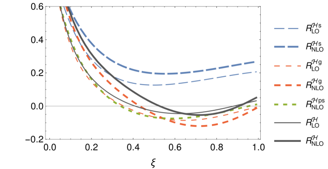
Figure 4: Relative error for the amplitude $\mathcal{H}$ from truncating the conformal partial wave expansion after the first term. We plot the $\xi$ dependence at $t=0$. Plotted quantities are defined in (44). The subscript denotes whether the leading order (LO) or next-to-leading order (NLO) coefficient function has been used. We have set $\kappa=1$ and $Q=\mu=2\,\text{GeV}$ corresponding to $\alpha_{s}=0.34$ (from (45)).

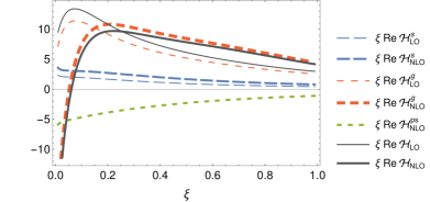
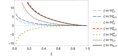
Figure 5: The real (left) and imaginary (right) parts of $\mathcal{H}$ at $\mu=2$ GeV separated into the $s$-quark, pure-singlet and gluon contributions. Results for both LO and NLO predictions are also shown.

It can be seen that the truncation error in the $s$-quark contribution is the largest, at best 20% around $\xi\approx 0.5$. The error does not decrease by increasing $\xi$, indicating that higher moments are important. Still, the situation is much better than in the Mellin moment expansion where the truncation error can be much larger Hatta and Strikman (2021). For the gluon and pure-singlet contributions, the threshold approximation is very good, with errors being below 10% starting already at $\xi\approx 0.35$. Interestingly, the approximation is the best for the total amplitude ${\cal H}$ for $\xi>0.5$, which may be a special feature of $\phi$-production. This is due to a significant cancellation between the $s$-quark and pure singlet contributions both in the truncated and full amplitudes, see the discussion below (37) and Fig. 5 where $\mathcal{H}^{s}_{\rm NLO}\approx-\mathcal{H}^{ps}_{\rm NLO}$ in the entire $\xi$ range. As a result, $\mathcal{H}$ is almost entirely dominated by the gluon contribution $\mathcal{H}\approx\mathcal{H}^{g}$. We expect that the threshold approximation gets even better as $\mu^{2}\sim Q^{2}$ is increased, since the GPDs approach their asymptotic limits.

An important question is whether the above conclusion, obtained at an unphysical point $t=0$, remains qualitatively valid in the phenomenologically relevant region $t\approx t_{min}$. Empirically, it is known that the gluon GPD and form factors fall faster with increasing $|t|$ than the quark counterparts Lukashin et al. (2001); Chekanov et al. (2005); Aaron et al. (2008). One can then imagine a scenario where the $\sum_{q}A_{q}$ term in (III.3) cancels the $A_{g}$ term (instead of the $A_{s}$ term as mentioned above) at large-$t$. If this rather accidental cancellation occurs, $R^{\rm tot}$ can become very large $|R^{\rm tot}|\gg 1$ due to a small denominator $|{\cal H}_{\rm trunc}|$ even though the threshold approximation works well for individual contributions $|R^{s,ps,g}|\ll 1$. In fact, this is what happens if one evaluates ${\cal H}$ using $H(x,\xi,t=t_{min}(\xi))$ and the default parameter set of the GK model Goloskokov and Kroll (2008). We however think that this is an artifact of the GK model which predicts a too rapid falloff of the gluon GPD and GFFs at large-$t$ as compared to the quark ones. A more reasonable estimate of the $t$-dependence may come from lattice QCD Hackett et al. (2024), where it was found that $\sum_{q}A_{q}(t)$ and $A_{g}(t)$ have quite similar $t$-dependencies. A simple numerical check using (37) and the parametrization of $A_{q,g}(t)$ obtained in Hackett et al. (2024) shows that the $A_{g}$ term safely dominates over the $\sum_{q}A_{q}$ term in (III.3) in the phenomenologically relevant region $|t|<2$ GeV². Therefore, for the moment we exclude the above scenario, although further investigations are certainly needed.

Another caveat is that the GK model that has been used here does not have a D-term, and hence no information about the $D$-type contributions in (III.3) can be gained from our analysis. However, the above discussion indicates that the dominance of the $j=1$ term is a generic feature at large skewness that arises from the combined effects of the suppression of the DGLAP region $\xi<|x|<1$, the smooth behavior of GPDs, and the property of the coefficient functions. Recalling that the $D$-term has support only in the ERBL region $|x|<\xi$, we can expect a similar level of accuracy after including the $D$-type contributions. The relative signs of the contributions might differ. For instance, we might have $D_{s}>0$ (whereas $D_{u+d+s}<0$), which reverses the aforementioned cancellation between the $s$-quark and pure-singlet contributions.

Overall, we conclude that errors due to the threshold approximation are at worst $20\%$ and can be as good as $10\%$ or less for moderately large $\xi\gtrsim 0.4$. Considering also the discussion around (25), it appears that the range $0.4<\xi<0.6$ is the best region to focus on.

IV Numerical analysis

In this section we present our numerical results on the differential cross section $\frac{d\sigma_{L}}{dt}$ (26), where ${\cal H},{\cal E}$ are given by (III.3), (III.3). The inputs for the NLO computation are as follows. The one-loop running coupling is

$$\alpha_{s}(\mu)=\frac{4\pi}{\beta_{0}\ln(\mu^{2}/\Lambda_{\rm QCD}^{2})},\qquad\beta_{0}=\frac{11N_{c}}{3}-\frac{2n_{f}}{3},$$ (45)

where $n_{f}=4$. Following Čuić et al. (2023), we set $\frac{\alpha_{s}}{2\pi}=0.0606$ at $Q^{2}=2.5$ GeV², which gives $\Lambda_{\rm QCD}^{2}=0.0476$ GeV². The $\phi$-meson decay constant is

$$f_{\phi}=0.221\,{\rm GeV},$$ (46)

as in Čuić et al. (2023). As for the GFFs, we use the dipole and tripole parameterizations for the $A$-type and $D$-type form factors, respectively Tanaka (2018); Tong et al. (2021)

$$A_{q,g}(t,\mu)=\frac{A_{q,g}(\mu)}{(1-t/m_{A}^{2})^{2}},$$ (47)

$$D_{q,g}(t,\mu)=\frac{D_{q,g}(\mu)}{(1-t/m_{D}^{2})^{3}}.$$

In principle, the mass parameters $m_{A}$ and $m_{D}$ depend on parton species, but for simplicity we assume common values Duran et al. (2023)

$$m_{A}=1.6\,{\rm GeV},\qquad m_{D}=1.1\,{\rm GeV}.$$ (48)

The forward values $A_{a}(\mu)$ represent the momentum fraction of the proton carried by partons $\sum_{a=q,g}A_{a}(\mu)=1$. We consider their one-loop QCD evolution using

$$A_{s}(\mu_{0})=0.03,\qquad A_{g}(\mu_{0})=0.42,\qquad A_{u+d+c}(\mu_{0})=1-A_{s}(\mu_{0})-A_{g}(\mu_{0}),$$ (49)

at the reference scale $\mu_{0}=2$ GeV Hou et al. (2021). The one-loop evolution of the D-terms $D_{q,g}(\mu)$ is the same as that for $A_{q,g}(\mu)$ and is explicitly given by

$$D_{q}(\mu) = \frac{D}{4C_{F}+n_{f}}+\frac{1}{n_{f}\left(4C_{F}+n_{f}\right)}\left(\frac{\alpha_{s}(\mu_{0})}{\alpha_{s}(\mu)}\right)^{-\frac{2}{3\beta_{0}}\left(4C_{F}+n_{f}\right)}\bigl{(}4C_{F}D-\left(4C_{F}+n_{f}\right)D_{g}(\mu_{0})\bigr{)}$$ (50)

$$+\left(\frac{\alpha_{s}(\mu_{0})}{\alpha_{s}(\mu)}\right)^{-\frac{8C_{F}}{3\beta_{0}}}\left(D_{q}(\mu_{0})-\frac{1}{n_{f}}\sum_{q^{\prime}}D_{q^{\prime}}(\mu_{0})\right),$$

$$D_{g}(\mu) = \frac{4C_{F}}{4C_{F}+n_{f}}D-\frac{1}{4C_{F}+n_{f}}\left(\frac{\alpha_{s}(\mu_{0})}{\alpha_{s}(\mu)}\right)^{-\frac{2}{3\beta_{0}}\left(4C_{F}+n_{f}\right)}\left(4C_{F}D-(4C_{F}+n_{f})D_{g}(\mu_{0})\right),$$ (51)

where the total D-term $D=\sum_{q}D_{q}(\mu)+D_{g}(\mu)$ is $\mu$-independent. Our main interests in this paper are the strangeness and gluon D-terms $D_{s}(\mu)$ and $D_{g}(\mu)$. We therefore assume that, at the reference scale $\mu_{0}=2$ GeV Hackett et al. (2024),

$$D_{u+d+c}(\mu_{0})=-1.2$$ (52)

and treat $D_{s}(\mu_{0})$ and $D_{g}(\mu_{0})$ as free parameters. In the following, we use the simpler notations $D_{s}(\mu_{0})\to D_{s}$ and $D_{g}(\mu_{0})\to D_{g}$. Finally, we neglect the $B$-type GFFs $B_{q,g}(t)$ altogether Teryaev (1999); Hagler et al. (2008).

\begin{overpic}[width=260.17464pt,trim=0.0pt 0.0pt 17.07182pt 42.67912pt,clip]{NLOVariation.pdf} \par\put(-6.0,20.0){\rotatebox{90.0}{\small$d\sigma_{L}/d|t|\;(\mathrm{nb}/\mathrm{GeV}^{2})$}} \par\put(45.0,-4.0){\small$|t|\;(\mathrm{GeV}^{2})$} \par\put(35.0,45.0){{\color[rgb]{0,0,0}\raisebox{3.22916pt}{\rule{15.00002pt}{2.0pt}}}\,\large{LO}} \put(35.0,50.0){{\color[rgb]{0,0,0}\raisebox{3.22916pt}{\rule{15.00002pt}{2.0pt}}}\,\large{NLO}} \par\end{overpic}

Figure 6: Differential $\gamma^{*}p$ cross section in units of nb/GeV² at $W=Q=2.5$ GeV, $D_{g}=-1$, and $D_{s}=0$ as a function of $|t|$. The orange and blue bands represent the LO and NLO cross sections, respectively, with the renormalization scale varied in the range $Q/2<\mu<2Q$.

\begin{overpic}[width=433.62pt,trim=0.0pt 0.0pt 17.07182pt 42.67912pt,clip]{Ds_HK_Edited.pdf} \par\put(-7.0,20.0){\rotatebox{90.0}{\small$d\sigma_{L}/d|t|\;(\text{nb}/\text{GeV}^{2})$}} \put(40.0,-4.0){\small$|t|\;(\text{GeV}^{2})$} \par\put(35.0,40.0){{\color[rgb]{0,0,0}\raisebox{3.22916pt}{\rule{15.00002pt}{1.5pt}}}\,\large$D_{s}=-1.0$ } \put(35.0,46.0){{\color[rgb]{0,0,0}\raisebox{3.22916pt}{\rule{15.00002pt}{1.5pt}}}\,\large$D_{s}=-0.5$ } \put(35.0,52.0){{\color[rgb]{0,0,0}\raisebox{3.22916pt}{\rule{15.00002pt}{1.5pt}}}\,\large$D_{s}=0.0$ } \end{overpic}

\begin{overpic}[width=433.62pt,trim=0.0pt 0.0pt 17.07182pt 42.67912pt,clip]{DgVariation.pdf} \par\put(-7.0,20.0){\rotatebox{90.0}{\small$d\sigma_{L}/d|t|\;(\text{nb}/\text{GeV}^{2})$}} \put(40.0,-4.0){\small$|t|\;(\text{GeV}^{2})$} \par\put(35.0,40.0){{\color[rgb]{0,0,0}\raisebox{3.22916pt}{\rule{15.00002pt}{1.5pt}}}\,\large$D_{g}=-2.0$ } \put(35.0,46.0){{\color[rgb]{0,0,0}\raisebox{3.22916pt}{\rule{15.00002pt}{1.5pt}}}\,\large$D_{g}=-1.0$ } \put(35.0,52.0){{\color[rgb]{0,0,0}\raisebox{3.22916pt}{\rule{15.00002pt}{1.5pt}}}\,\large$D_{g}=0.0$ } \par\end{overpic}

Figure 7: NLO longitudinal cross section at $W=Q=2.5$ GeV as a function of $|t|$. Left: $D_{s}=0,-0.5,-1$ from top to bottom at fixed $D_{g}=-1$. Right: $D_{g}=0,-1,-2$ from top to bottom at fixed $D_{s}=0$.

We are now ready to present the numerical results. First, the differential cross section (26) at $W=Q=2.5$ GeV, $D_{g}=-1$, $D_{s}=0$ is shown in Fig. 6. The purple and yellow lines represent the LO and NLO cross sections evaluated at $\mu=Q$, respectively. The orange and green bands are the respective uncertainty bands obtained by varying $\mu$ in the range $Q/2<\mu<2Q$. As expected, the scale uncertainty is reduced by going to NLO. The result in the large-$|t|$ region should be taken with a grain of salt because higher twist corrections might be very large there. In the present kinematics, the condition (22) reads $|t|\lesssim\frac{Q^{2}}{3}\approx 2.1$ GeV.

Next, in Fig.7 we show $\frac{d\sigma_{L}}{dt}$ at NLO for three different values of $D_{s}$ at fixed $D_{g}$ (left) and for three different values of $D_{g}$ at fixed $D_{s}$ (right). Again, the band attached to each curve represents the scale uncertainty $Q/2<\mu<2Q$. (The same comment applies to the plots below and will not be repeated.) It is reassuring to see that the sensitivities to $D_{s,g}$ are larger than the theory uncertainty bands, making this observable ideally suited for constraining $D_{s,g}$. As we increase $W$, the three curves tend to approach one another. But they are still well separated when $W\lesssim 3$ GeV, which is the limit of applicability of our calculation, see below. The bending of $d\sigma/dt$ in the small-$|t|$ region for large negative values of $D_{s}$ was previously observed in Hatta and Strikman (2021). We note that a recent model calculation found $D_{s}\approx-0.5$ Won et al. (2023).

In Fig. 8 (left), we plot the integrated cross section

$$\sigma_{L}(W,Q)=\int_{t_{min}}^{t_{max}}dt\frac{d\sigma}{dt},$$ (53)

at fixed $Q=2.5$ GeV. Again, the integrand in the large-$t$ region is not reliable due to potentially large higher twist corrections. Fortunately, however, the integral is dominated by the small-$t$ region $t\sim t_{min}$. Due to the spin-2 nature of the energy momentum tensor, the cross section rises rather fast with increasing $W$. While this is a definite prediction of theory near the threshold, the strong dependence on $W$ cannot be extrapolated to high-$W$ values. A comparison with the experimental data taken at high energy (such as at HERA, see below) suggests that already $W=3$ GeV is too high to be considered within the threshold region. We feel comfortable applying our result to, say, $W\lesssim 2.8$ GeV.

Finally, in Fig. 8 (right), we plot the $Q$-dependence of the NLO integrated cross section (53) at fixed $W=2.5$ GeV. We find that the cross section falls very rapidly with increasing $Q$ as

$$\sigma_{L}\propto\frac{1}{Q^{a}},\qquad 9<a<10.$$ (54)

At first sight, this is surprising because superficially the formula (26) suggests that, at fixed $W$,

$$\frac{d\sigma_{L}}{dt}\propto\frac{1}{Q^{4}}\qquad(Q^{2}\to\infty).$$ (55)

Two powers of $1/Q$ come from the hard coefficients (33) squared, and the remaining factor $1/Q^{2}$ comes from $p_{cm}\sim Q^{2}$ at high-$Q^{2}$. The extra suppression (54) mainly comes from the gravitational form factors. As mentioned earlier, $t_{min}$ grows quadratically with $Q$

$$|t_{min}|=a(W)Q^{2}+\cdots,$$ (56)

already when $Q\gtrsim 2$ GeV. Although the coefficient $a$ is small in the sense of (22), (56) eventually leads to the behavior

$$A_{g}(t)\propto\frac{1}{(t-m_{A}^{2})^{2}}<\frac{1}{(t_{min}-m_{A}^{2})^{2}}\sim\frac{1}{Q^{4}},$$ (57)

which partly explains (54). Typically in high energy experiments, one measures the region $|t|\lesssim 1$ GeV² and does not expect any correlation between $t$ and $Q^{2}$. While the faster-than-expected falloff (54) is a unique feature of near-threshold production, it also makes measurements at high-$Q^{2}$ challenging.

\begin{overpic}[width=433.62pt]{WVariation.pdf} \put(-7.0,30.0){\rotatebox{90.0}{\small$\sigma_{L}\;(\text{nb})$}} \put(40.0,-4.0){\small$W\;(\text{GeV})$} \end{overpic}

\begin{overpic}[width=433.62pt]{QVariation.pdf} \put(-7.0,30.0){\rotatebox{90.0}{\small$\sigma_{L}\;(\text{nb})$}} \put(40.0,-4.0){\small$Q\;(\text{GeV})$} \end{overpic}

Figure 8: NLO longitudinal cross section integrated over $t$ with $D_{s}=0$ and $D_{g}=-1$ as a function of $W$ at fixed $Q=2.5$ GeV (left) and as a function of $Q$ at fixed $W=2.5$ GeV (right). The orange dashed curve is the CLAS parametrization (58).

V Experimental Projections for the EIC and JLab

We turn now to determining whether the restrictive kinematic requirements laid out in the previous sections can be feasibly satisfied by an experiment. To summarize these requirements, the value of $Q^{2}$ should be a factor of 3 or more greater than $|t|$, $\xi$ should be greater than 0.4, and $W$ should be less than 3 GeV. To explore the sensitivity of various experiments, we utilize the lAger Monte Carlo event generator, which is capable of simulating a variety of exclusive reactions in both photoproduction and electroproduction Joosten (2021).

In Monte Carlo simulations, events with all possible values of $W,Q^{2}$ are generated. Also, the virtual photon can be both transversely and longitudinally polarized. In contrast, our perturbative calculation is valid only near the threshold (low-$W$) and at high-$Q^{2}$, and only for the longitudinally polarized photons. Increasing $W$ is roughly equivalent to decreasing skewness $\xi$. If we require $\xi>0.4\sim 0.5$, Fig. 1 already suggests that we cannot go much higher than $W\sim 3$ GeV. To estimate at which value of $Q$ our result becomes unreliable, in Fig. 8 we have also plotted (dashed curve) the following parametrization of world data by the CLAS collaboration Avakian et al. :

$$\sigma^{\rm CLAS}_{L}(W,Q)=R(Q)\sigma^{\rm CLAS}_{T}(W,Q),\qquad\sigma^{\rm CLAS}_{T}(W,Q)=400\left(1-\frac{W_{th}^{2}}{W^{2}}\right)\frac{W^{0.32}}{\left(1+\frac{Q^{2}}{M_{\phi}^{2}}\right)^{3}},$$ (58)

where $W,Q$ are in units of GeV and the $L/T$ ratio is assumed to be $W$-independent

$$R(Q)=\frac{0.4Q^{2}}{M_{\phi}^{2}}.$$ (59)

A more recent and more elaborate parametrization of $R$ from the HERA data can be found in Čuić et al. (2023). (58) features the usual scaling relation $d\sigma_{L}\sim 1/Q^{4}$ (55) at high-$Q^{2}$ as well as a Pomeron-like behavior (gradual increase with $W$) at high-$W$. These constraints mainly come from the HERA data at high-$W$. On the other hand, at low-$W$, the fit is poorly constrained due to the scarcity of electroproduction data. In particular, the CLAS data Santoro et al. (2008) are limited to $Q^{2}<3.8$ GeV².

The right plot of Fig. 8 suggests that our formula can be used at $Q\gtrsim 2.4$ GeV. Below this scale, it appears necessary to tame the singular behavior $1/Q^{2}$ in the perturbative kernel. The left plot provides another argument that indeed the threshold approximation is limited to $W\lesssim 3$ GeV. In order to implement this transition in our simulation, we evaluate the cross section in a given point in phase space by the smaller of the two

$${\rm min}\{\sigma^{\rm CLAS},\sigma^{\rm pQCD}\}.$$ (60)

More precisely, to facilitate the implementation we have parametrized the NLO cross section in the form

$$\sigma^{\rm pQCD}_{L}(W,Q)=\frac{140}{Q^{9.4}}(W^{2}-1.96^{2})^{0.71}W^{3.8}.$$ (61)

Notice the very different $W$- and $Q$-dependencies from (58) as already discussed. We then apply the same $R$-factor (59) to (61) to obtain a model for $\sigma_{T}^{\rm pQCD}$ and hence also the sum (16). We further assume the following $t$-dependence motivated by the dipole form factor (47)

$$\frac{d\sigma_{T/L}}{dt}=\frac{3(m_{g}^{2}-t_{min})^{3}}{(m^{2}_{g}-t)^{4}}\sigma_{T/L},$$ (62)

where $m_{g}=1$ GeV in the CLAS model Avakian et al. and $m_{g}=m_{A}=1.6$ GeV (48) in our model. In this way, we evaluate (60) at the level of the differential cross section $\frac{d\sigma}{dt}$ and generate events according to this probability.

In practice, an actual experiment will measure the $e+p$ cross section within a certain kinematic range and then extract the longitudinal cross section using the formula (16). While one may use a model for $R$ as in our simulations, $R$ can be experimentally determined if the spin-density matrix elements (SDMEs) of the $\phi$ are measured. Assuming $s$-channel helicity conservation (SCHC), the value of $R$ is given as

$$R=\frac{T_{00}^{2}}{T^{2}_{11}}=\frac{1}{\varepsilon}\frac{r^{04}_{00}}{1-r^{04}_{00}},$$ (63)

in the Schilling and Wolf convention Schilling and Wolf (1973), where $T_{00}$ and $T_{11}$ are the helicity amplitudes for a longitudinally polarized photon to transition to a longitudinally polarized vector meson and a transversely polarized photon to transition to a transversely polarized vector meson, respectively. $r^{04}_{00}$ is the dominant spin-density matrix element describing the longitudinal photon to longitudinal vector meson transition and is measurable from the angular distribution of the $\phi$ decay products. In light of the violation of SCHC observed by some experiments, the H1 experiment Aaron et al. (2010) employed a more rigorous formula than (63) and measured $R$ in bins of $Q^{2}$ with a precision of approximately 10% at values of $Q^{2}$ similar to those relevant here. In principle, the value of $R$ can be determined for each bin in $x_{B},Q^{2},W,$ and $t$ independently if the statistical and systematic uncertainties in the bin are small enough to permit measurement of SDMEs. This should be possible with SoLID at JLab and the EIC at BNL, the future large-acceptance experiments that will be able to detect the $\phi$ decay products. For this reason, in the following subsections we provide projections for the measurement of the longitudinal cross section at SoLID and the EIC.

V.1 EIC

The major challenge for measuring near-threshold meson production at a collider arises from the fact that the produced meson and the scattered proton must be relatively close in momentum and angle. This means that for events with $W\approx W_{th.}$, the meson decay products are generally lost down the beampipe. This limited the H1 and ZEUS measurements of exclusive $\phi$ production to $W>35$ GeV. However, the flexibility of the EIC in terms of beam energies and the large detector acceptances provide the first opportunity to measure near-threshold meson production at an $e+p$ collider.

The ePIC experiment will be operational at the beginning of EIC running and located at the 6 o’clock interaction point. ePIC offers excellent acceptance and capability for measuring the momentum and species of long-lived particles such as pions, kaons, and protons. To make projections for measurements of exclusive $\phi$ electroproduction we will assume acceptances, resolutions, and particle identification abilities similar to what should be achieved by ePIC, summarized in Table 1 ePIC Collaboration (2025). However, it is worth noting that a second EIC detector, coming online after ePIC and the first phase of EIC running, could offer improved capabilities for these measurements. The configuration of the EIC which collides 5 GeV electrons with 41 GeV protons (5x41) offers the best experimental access to the near-threshold region because the charged kaons produced in the decay of the $\phi$ enter the central detector region of $-3.5<\eta<3.5$. These $\phi$ decay kaons predominantly populate the forward region of the detector, where ePIC is equipped with a dual-radiator Ring-Imaging Cherenkov (dRICH) detector capable of efficiently separating pions from kaons up to approximately 50 GeV Chatterjee (2024). For the purposes of this study, we assume that the dRICH and time-of-flight system can provide perfect identification of kaons from $\phi$ decay, which have typical momenta of 5 GeV.

The momentum spectra of all four final-state particles in reconstructed near-threshold events are shown in Fig. 9. The scattered electron and the kaons from the $\phi$ decay are required to be within the central detector acceptance $|\eta|<3.5$. In near-threshold events, the scattered proton is most often measured in the B0 detector system, which spans approximately $4.6<\eta<5.9$. However, the azimuthal angle acceptance of the B0 is not 100% for all polar angles. To compensate for the missing azimuthal acceptance, the assumed detection efficiency of the B0 detectors is set to 70%. Finally, at the smallest scattering angles, the proton can be detected in the Roman Pots (RP) or Off-momentum Detectors (OMD), which reside inside the beam vacuum. Since these detectors rely on particles passing through the accelerator magnet optics along certain trajectories, they do not have acceptance for all momenta. To crudely simulate this effect, we include a longitudinal momentum dependent acceptance of $0.65<p_{z}/p_{\mathrm{beam}}<1$ and $0.3<p_{z}/E_{\mathrm{beam}}<0.6$. There will also be a dependence of the acceptance on $p_{T}$, which we make no attempt to capture here. We also note that the above numbers hold for the 18x275 magnet lattice, but the acceptance will likely change in the 5x41 magnet lattice. A second detector at the EIC will have a still-different lattice and may make use of a second focus point in the accelerator magnets to significantly enhance the RP/OMD acceptance. The present assumption of 95% efficiency in the RP/OMD is optimistic. However, for the range of $W$ that we focus on, namely $2.4<W<2.8$, less than 10% of scattered protons are produced at $\eta>5.9$. We therefore expect our results to hold regardless of the details of the RP/OMD acceptance.

The momentum resolutions of the central, B0, and RP/OMD sections of the detector are in line with what can be expected from ePIC. The angular resolutions are somewhat less studied than the momentum resolutions. We posit that the angular resolution of the B0 and RP/OMD detectors, all of which are equipped with high resolution tracking detectors, will be somewhat better than the central detector due to the significantly longer distance that particles travel before interacting with the far-forward detectors. The number of 3 mrad is perhaps conservative for the central detector as a whole, but as can be seen from Fig. 9, most of the electrons and kaons do enter the central detector at relatively steep angles where the angular resolution is expected to deteriorate somewhat.

Detector Region	Efficiency	Momentum Resolution	Angular Resolution
Central $(|\eta|<3.5)$	95%	$\displaystyle\frac{\Delta p}{p}=\begin{cases}1\%,&|\eta|<2.5\\ 2.5\%,&2.5<|\eta|<3.5\\ \end{cases}$	$\displaystyle\sigma_{\theta,\phi}=3\,\text{mrad\quad}$
B0 $(4.6<\eta<5.9)$	70%	$\displaystyle\frac{\Delta p_{T}}{p_{T}}=6\%$	$\displaystyle\sigma_{\theta,\phi}=1\,\text{mrad\quad}$
RP/OMD $(\eta>6.0)$	95%	$\displaystyle\frac{\Delta p_{T}}{p_{T}}=8\%$	$\displaystyle\sigma_{\theta,\phi}=1\,\text{mrad\quad}$

Table 1: Efficiencies, momentum resolution, and angular resolution in different pseudorapidity regions. The combined acceptance of the Roman Pots and Off-momentum detectors has an additional requirement that $\theta<5\,\text{mrad}$ and $p_{z}/p_{\mathrm{beam}}\in[0.65,1.0]\cup[0.3,0.6]$.

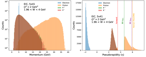
Figure 9: Momentum (Left) and pseudorapidity (Right) distributions for particles in events with $1.96<W<4$ GeV and $Q^{2}>2$ GeV² where all four final-state particles are reconstructed.

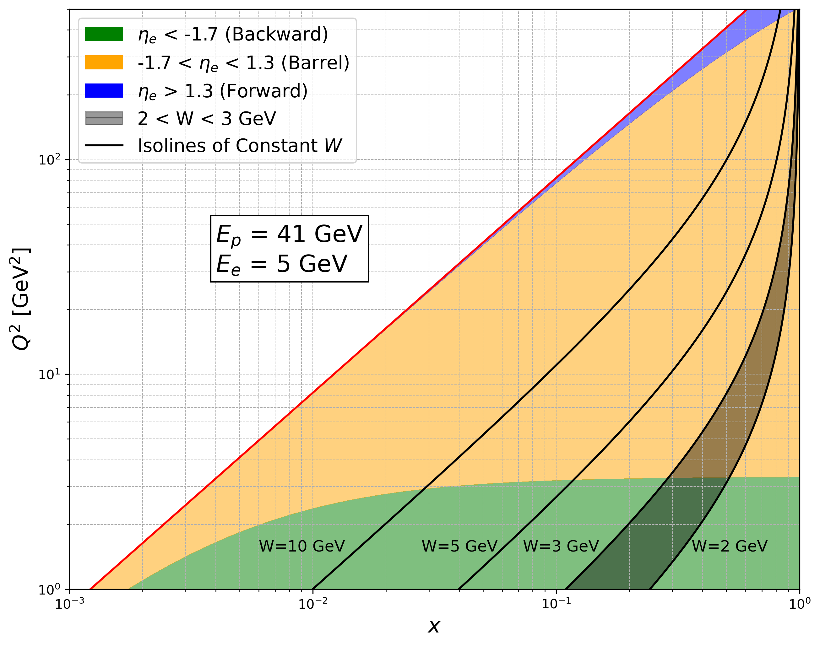
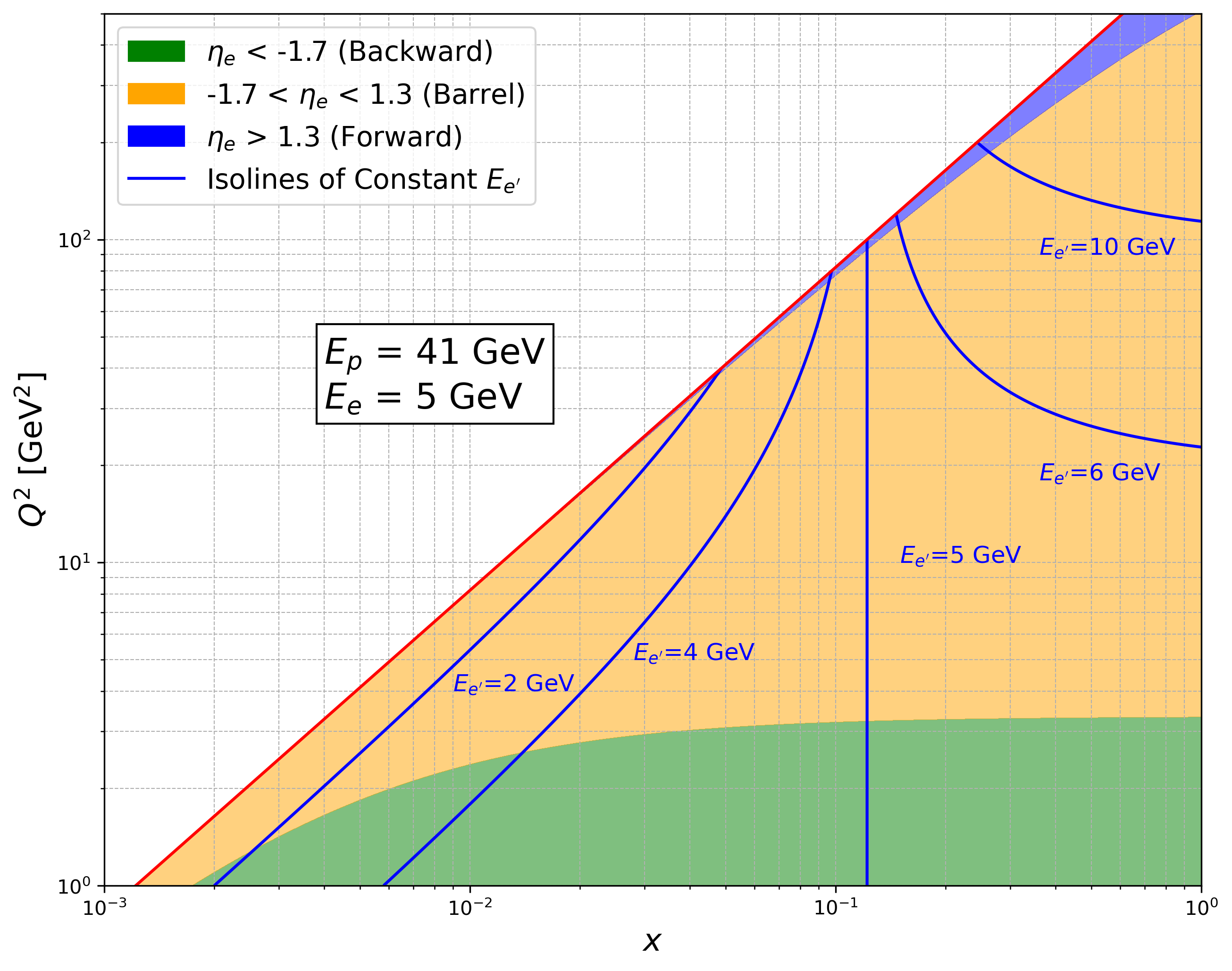
Figure 10: $x_{B},Q^{2}$ plane for the 5x41 beam energy configuration of the EIC. Left: Kinematic plane with iso-lines of constant $W$. The region of interest, $W<3$ GeV, is shaded in gray. Right: Kinematic plane with iso-lines of constant scattered electron energy $E_{e^{\prime}}$.

A key challenge in reconstructing near-threshold events at the EIC is accurately measuring the event kinematics. Relying solely on the scattered electron yields poor resolution at low $W$ because small mis-measurements of the electron energy can lead to large uncertainties in the reconstructed kinematic variables, as can be seen from the right panel of Fig. 10. In contrast, reconstructing the entire hadronic final state—the approach assumed in these projections—significantly improves the $W$ resolution from about 50% down to a few percent. When all final-state particles are measured, the full suite of inclusive kinematic reconstruction techniques (see Ref. Bassler and Bernardi (1995) for a succinct review) can be used to reconstruct $W$ via $Q^{2}$ and $x_{B}$ to great effect. Beyond these standard methods, $W$ can also be reconstructed as the invariant mass of the hadronic final state, potentially achieving even better resolution. Furthermore, the exclusivity of the events provides additional constraints that can be leveraged through kinematic fitting or ML-based approaches, leading to more precise event reconstruction overall.

The current projection for the EIC is that the integrated luminosity per year will be 5 fb^-1 for the 5x41 beam energy configuration. We assume in our projections a total integrated luminosity of 10 fb^-1, corresponding to approximately two years of 5x41 running. The 10x100 beam energy configuration offers a factor of 10 higher instantaneous luminosity, making it an attractive option. However, for the 10x100 beam energy, in the near-threshold kinematics the produced kaons almost exclusively fall in the pseudorapidity region $3.5<\eta<4.6$. In ePIC this pseudorapidity range is occupied primarily by the beampipe and is not instrumented with tracking and paricle identification. A second EIC detector with forward tracking and PID acceptance out to $\eta=4$ or greater could recover a significant fraction of these events and perhaps do a more precise measurement at the 10x100 beam energy.

Using the acceptances provided in Table 1 for the 5x41 configuration, the acceptance for events with $W<3$ GeV to be reconstructed with all four final-state particles is around 4%. The overall acceptance is primarily hindered by the acceptance for the scattered proton. We assume in our results a 10% systematic uncertainty, likely to arise from the understanding of the acceptance. This may be an underestimate, but this uncertainty will necessarily depend on the final implementation and performance of the subdetectors. An enhancement in the event statistics can be gained by not requiring the proton to be detected and instead using only the electron and kaons to reconstruct the event, but this comes at the cost of higher backgrounds and worsened resolution.

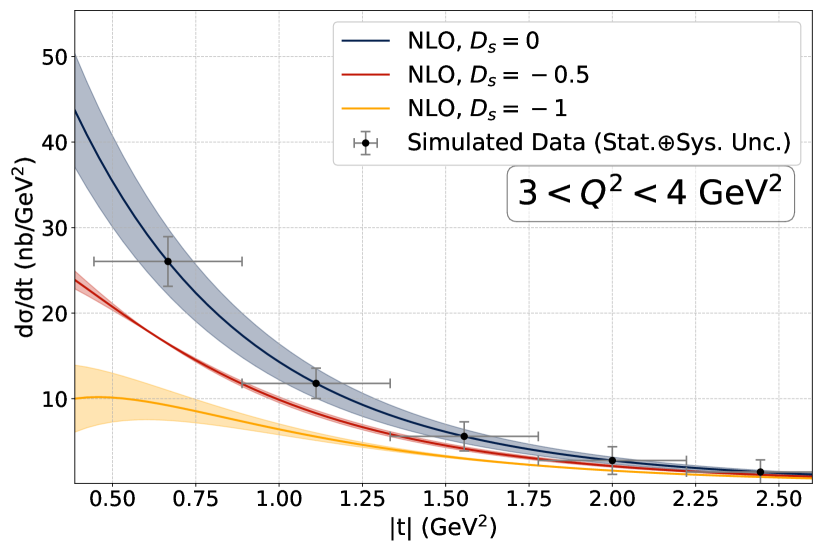
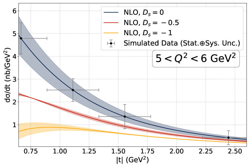
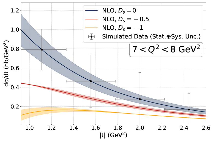
Figure 11: Projected results at the EIC for the cross section $\gamma^{*}_{L}+p\rightarrow\phi+p$ differential in $|t|$ and $Q^{2}$ in the near-threshold regime of $2.4<W<2.8$. The data points are fixed to the central value of the theoretical curve. Theoretical uncertainties are determined via a scale variation in the same way as Fig. 6. The assumed integrated luminosity is 10 fb^-1 at the 5x41 beam energy.

The projected sensitivity to $d\sigma_{L}/d|t|$ at the EIC is shown in Fig. 11. For simplicity, the NLO theory curves are generated at fixed values of $W$ and $Q^{2}$ corresponding to the center of the bin, i.e. $W=2.6$ GeV and $Q^{2}=3.5$ GeV² for the lowest $Q^{2}$ bin. The reconstructed fully exclusive event yield is around 1500 in 10 fb^-1 for $2.4<W<2.8$ GeV and $Q^{2}>3$ GeV². In all bins, the statistical uncertainty is larger than the assumed 10% systematic uncertainty. We present our results only in the range $2.4<W<2.8$ GeV because this range provides the best discriminating power for $D_{s}$. At lower $W$, the event statistics are too small to perform a reliable measurement of the $|t|$-distribution. At larger $W$, despite the somewhat higher measured event statistics, the sensitivity to $D_{s}$ is diminished. Besides, as explained before, our calculation is not reliable for $W>3$ GeV. Therefore we predict that $2.4<W<2.8$ GeV will be an optimal range for this measurement if the B0 detector meets the performance presented in Table 1 and the acceptance of the forward particle identification is not significantly reduced compared to the nominal $\eta<3.5$ boundary.

In summary, we present the first estimates for measuring near-threshold electroproduction of $\phi$ mesons at the EIC. Our preliminary calculations, based on naive assumptions about detector acceptances and resolutions, indicate that such a measurement is feasible. However, because event statistics at high $Q^{2}$ are low, extracting $D_{s}$ with high precision is challenging using only the nominal EIC detector acceptances. This measurement can be incrementally improved by collecting more than 10 fb^-1 of integrated luminosity at the 5x41 GeV beam energy. However, to achieve substantial gains in precision, the forward and far-forward detector acceptances need to exceed what was assumed here. A second EIC detector at IP8, optimized for exclusive measurements and leveraging the IP8 second focus, with forward particle identification out to $\eta=4$ (approximately a $2\degree$ polar angle), could exploit the higher luminosities available at higher beam energies and enable a much more precise measurement.

V.2 SoLID

At JLab, the future SoLID program in Hall A provides the luminosity, particle identification, and acceptance needed to perform precise measurements of rare processes. An experiment to study electroproduction of $\phi$ mesons in SoLID could run concurrently with the already approved SoLID $J/\psi$ experiment. The $J/\psi$ experiment plans to take 50 days of physics running with an 11 GeV $e^{-}$ beam at a current of 3 $\mu$A on a 15cm long LH₂ target, producing an instantaneous luminosity of approximately 10³⁷ cm^-2/s and collecting an integrated luminosity of 43.2 ab^-1. To evaluate SoLID’s capabilities for this measurement, we simulated 43.2 ab^-1 of $Q^{2}>2$ GeV² events using lAger at a beam energy of 10.6 GeV. A comprehensive summary of the SoLID detector is provided in Ref. Arrington et al. (2023).

SoLID consists of two annular sections covering the whole azimuth, known as the forward-angle detector (FAD) and the large-angle detector (LAD). As shown in Fig. 12, the FAD is equipped with GEM tracking planes, a light gas Cherenkov detector for separation of electrons and pions, a heavy gas Cherenkov detector for separation of pions from kaons, a time-of-flight layer for identification of protons and low momentum hadrons, and an electromagnetic calorimeter. The LAD is equipped with tracking, a scintillator layer for separation of electrons from photons, and electromagnetic calorimetry. The FAD covers the region of polar angle from $8\degree$ to $15\degree$ and the LAD covers $15\degree$ to $24\degree$, where polar angle is defined with respect to the center of the target.

The SoLID data acquisition system will be designed to handle a trigger rate of up to 100 kHz, motivated by the expected trigger rate for the SIDIS experiments. The trigger planned for the $J/\psi$ experiment is a triple coincidence of the scattered electron and an electron+positron pair from the decay of the $J/\psi$. The trigger rate for this topology is around 800 Hz, leaving ample room for additional triggers to run in parallel. Fully reconstructible near-threshold $\phi$ events occur on the order of 100 Hz, but the selection of these events at trigger-level is complicated by the large rate of random coincidences. Using a quadruple coincidence of an electron, identified via a high energy cluster in the large-angle calorimeter, and three charged hadrons, identified via hits in the scintillators and calorimeter, the trigger rate was roughly estimated to be around 100 kHz. A reduction of the trigger rate to acceptable levels without prescaling could be achieved if even rudimentary tracking information could be included in the trigger. Still further improvements could be gained by moving to a software-based trigger system. A software trigger permits real-time reconstruction, allowing advanced analysis cuts such as two-track invariant mass to be implemented in the trigger. The ability to place analysis cuts at trigger-level enables utilizing the powerful constraints imposed by the exclusivity of the process to completely eliminate random coincidences. This paradigm has been demonstrated at large-scale by the LHCb collaboration Aaij et al. (2019) in a complex detector system not unlike SoLID. Such an upgrade to the data acquisition system would be highly beneficial for the study of exclusive $\phi$ production and the SoLID physics program overall, allowing SoLID to make full use of the unparalleled combination of luminosity and acceptance without the otherwise strict limitations imposed by random coincidence trigger rates. This upgrade route furthermore has synergies with the High Performance Data Facility (HPDF) led by Jefferson Lab. In the projections provided in this section, we assume an un-prescaled data acquisition system capable of reading out all $\phi$ events. All of this being said, a trigger prescale of a factor of two would not substantially endanger the measurement, as will be shown in the remainder of this section.

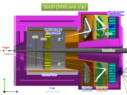
Figure 12: The SoLID detector in the configuration planned for the $J/\psi$ and SIDIS experiments. Image reproduced from Ref. Arrington et al. (2023)

The resolutions and detector acceptances assumed in this study were determined by the SoLID collaboration with a dedicated GEANT4 simulation in the GEMC framework GEMC (started 2007); libsolgem (started 2011); SOLID_GEMC (started 2010); SoLIDTracking (started 2016); Allison et al. (2016). We make use of these results in a fast MC to smear the four-vectors of generated particles in accordance with the expected resolutions. The acceptance of the SoLID $J/\psi$ configuration in momentum and polar angle $\theta$ is shown in Fig. 13. The fast MC queries the acceptance map and randomly discards or accepts particles based on their momentum and polar angle in accordance with the expected acceptance. Compared to the acceptance map determined with the SoLID GEANT4 simulation, for the purposes of making realistic projections we scale the acceptance by a factor of 0.9 to simulate tracking inefficiencies in the high-rate environment at SoLID. We furthermore only consider events in which the proton and kaons enter the FAD, such that they can be efficiently identified by the particle identification detectors. We assume perfect identification of kaons and protons in the FAD, which should be a reasonable approximation since background pions can be rejected by the heavy gas Cherenkov and protons can be identified by the time-of-flight.

Since statistical uncertainty is less of a limitation at SoLID, the bin sizes in $|t|,W,$ and $Q^{2}$ were chosen to be a factor of 3 or more larger than the detector resolution on those quantities. This should permit a reasonably stable unfolding and bin-by-bin extraction of $R$. To approximate the effect of systematic uncertainties, we assume a uniform systematic uncertainty of 10% on each bin of $|t|$.

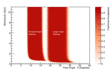
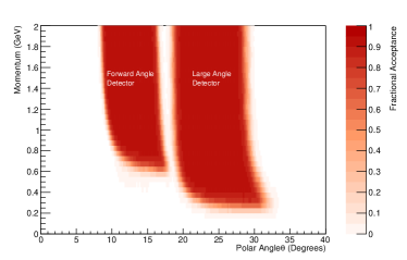
Figure 13: The fractional acceptance of SoLID for charged particles in momentum and polar angle. Left: Full acceptance for particles of momenta up to 11 GeV. Right: Zoomed acceptance for particles in the momentum range particularly relevant for reactions at low values of $|t|$.

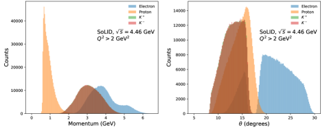
Figure 14: Momentum (Left) and polar angle (Right) distributions for particles in fully reconstructed events with $1.96<W<4$ GeV and $Q^{2}>2$ GeV². The gap between the forward-angle and large-angle detectors is visible around 16 degrees.

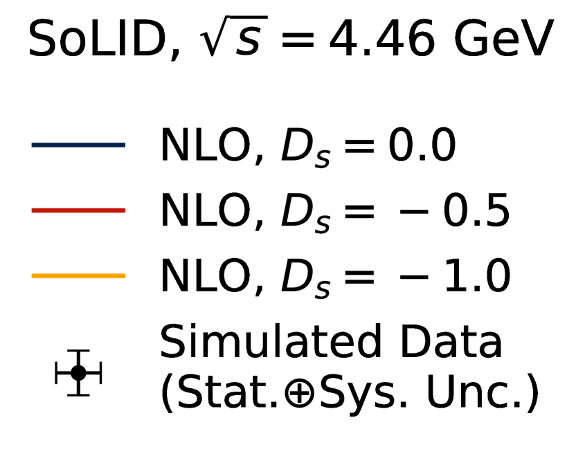
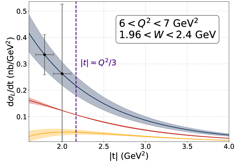
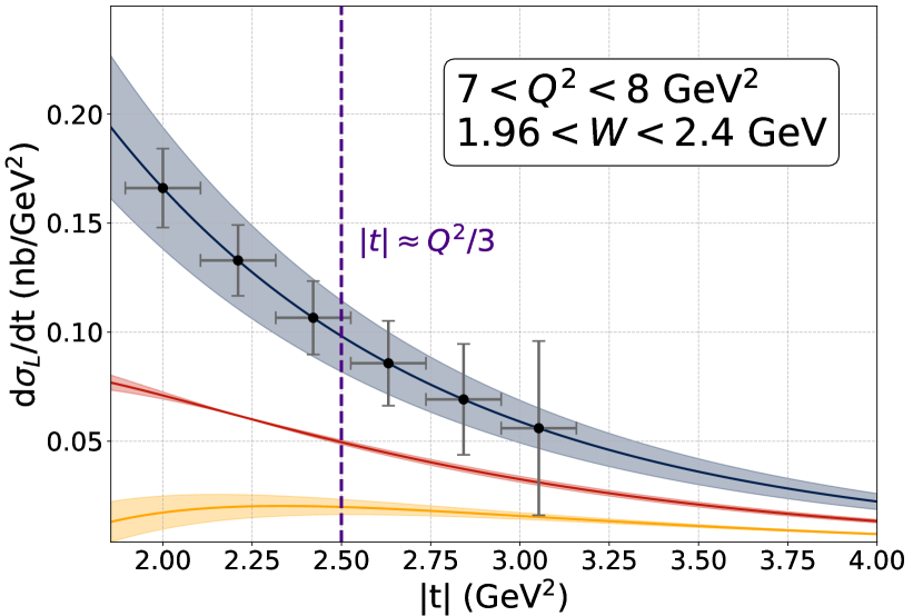
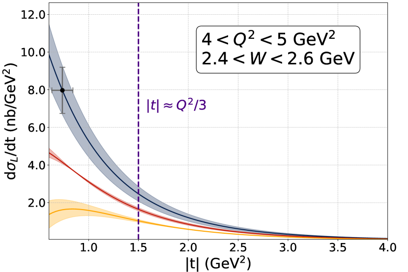
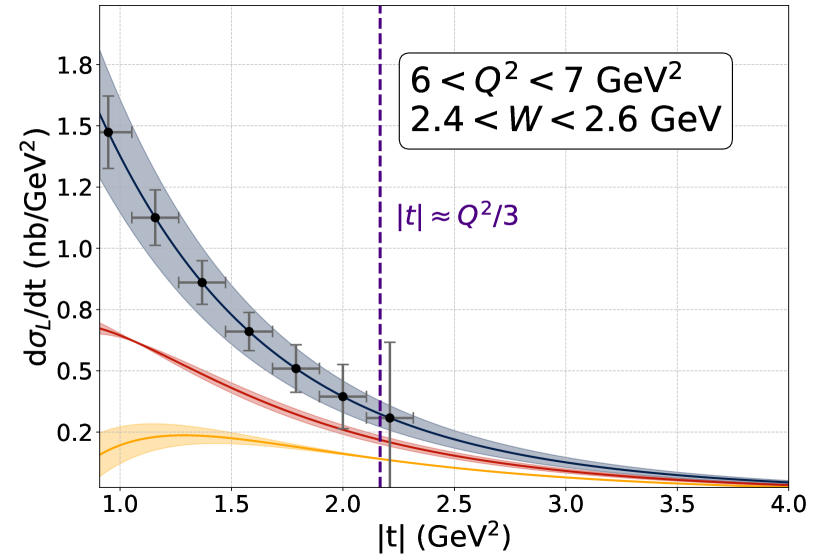
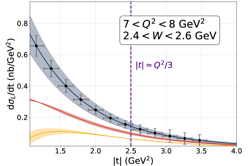
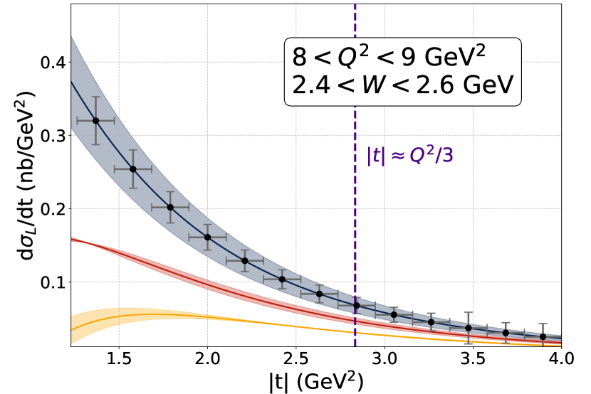
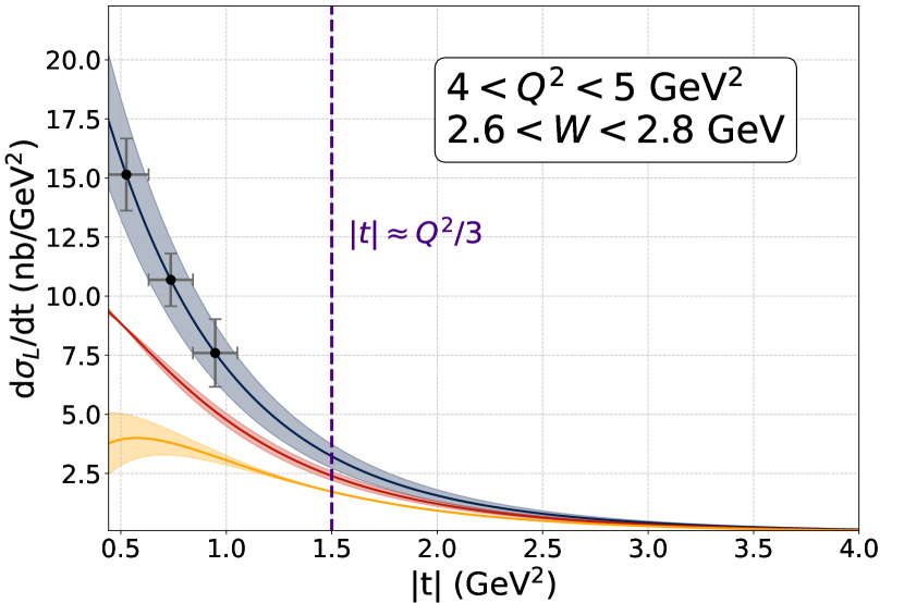
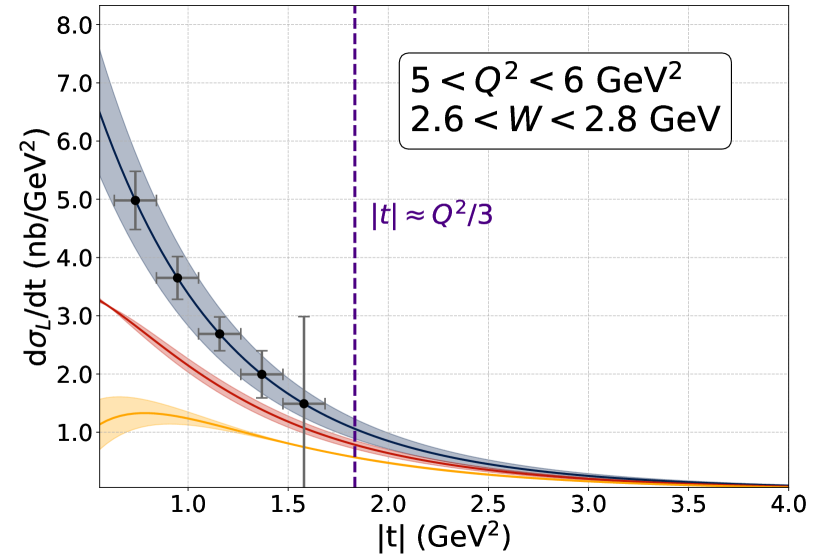
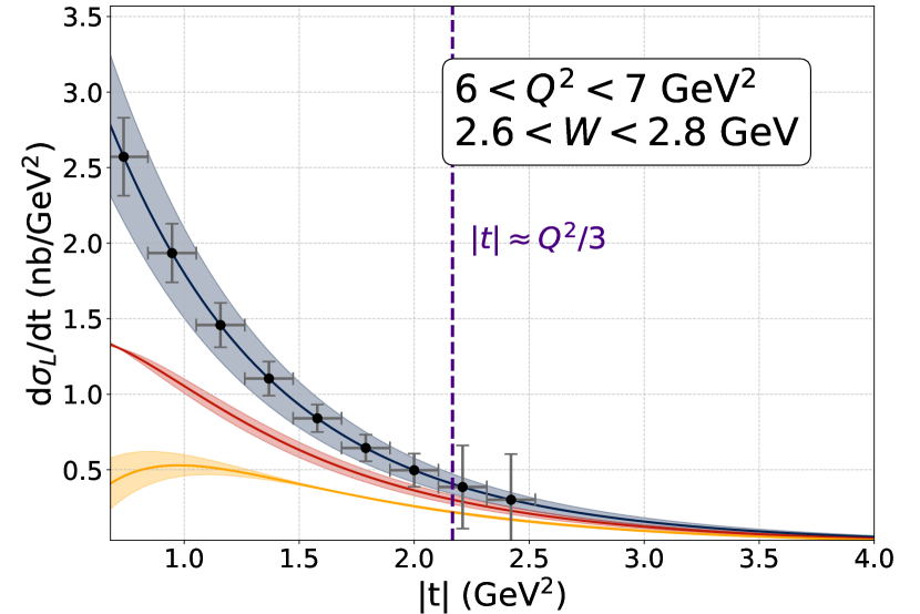
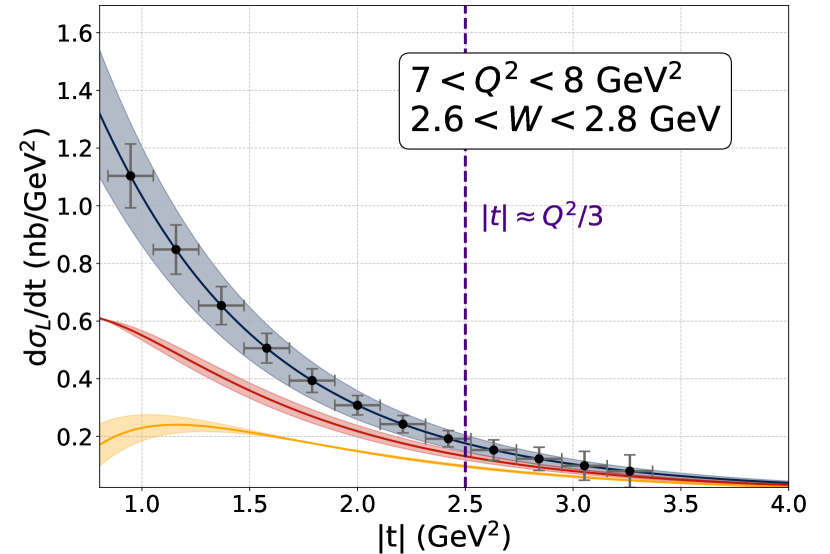
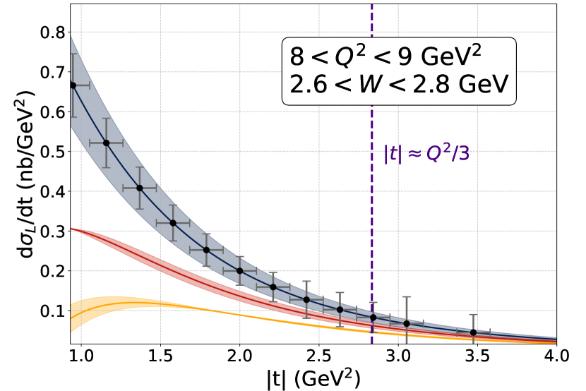
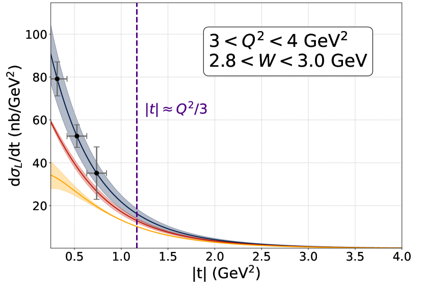
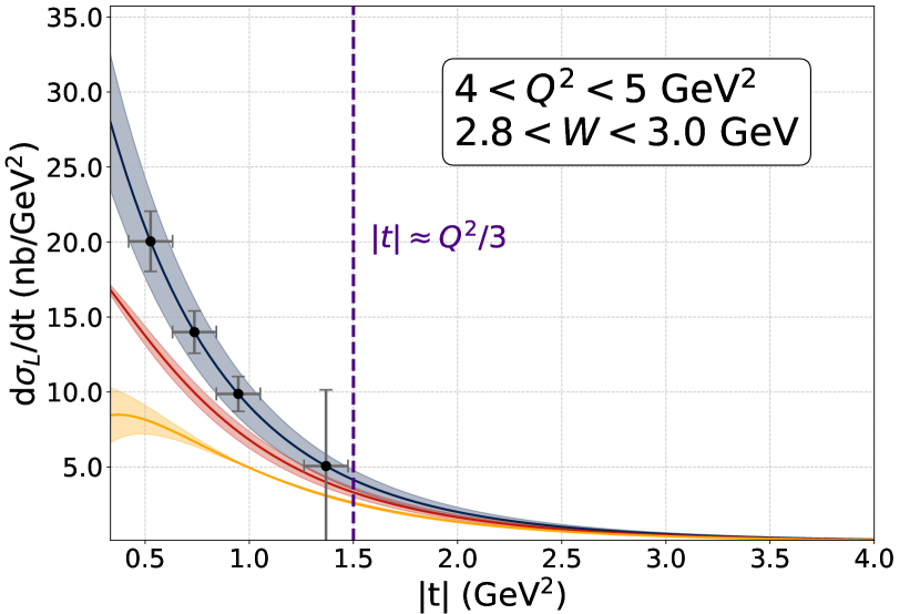
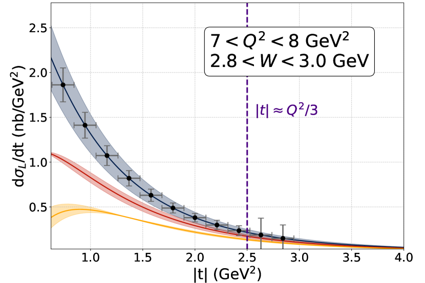
Figure 15: Projected results at SoLID for the $\gamma^{*}_{L}+p\rightarrow\phi+p$ cross section, differential in $|t|$ and $Q^{2}$ in the near-threshold regime. The assumed integrated luminosity is 43.2 ab^-1. The first (leftmost) column shows 4 $Q^{2}$ bins for $W=2.18$, while the subsequent columns each represent a bin in $W$ with five $Q^{2}$ bins. Note that the accessible range in $Q^{2}$ changes in each column due to the kinematic dependence on $W$. The purple dashed line is drawn at $|t|\approx Q^{2}/3$, where $Q^{2}$ is assumed to be the bin center.

For comparison with the results for the EIC, in the range of $2.4<W<2.8$ GeV and $Q^{2}>3$ GeV², we project that SoLID will reconstruct around 270,000 events with all four final-state particles being detected. The SoLID acceptance in the near-threshold region ($W<2.8$ GeV) depends strongly on $Q^{2}$, ranging from almost 10% for events with $7<Q^{2}<8$ GeV² to around 0.2% for $3<Q^{2}<4$ GeV². Similarly to the EIC, the kinematic reach and event statistics can be improved beyond what is presented here if only three of the four final-state particles are required to be detected. Another possible way to improve the statistics is to reconstruct the final state $e^{\prime},p,$ and $K_{s}^{0}$ from the $\phi\rightarrow K_{s}^{0}K^{0}_{L}$ decay and infer the $K^{0}_{L}$ from missing mass. As in Fig. 11, the theory curves are generated at the bin centers in $Q^{2}$ and $W$. Due to the form factor of (62), the highest statistics are available at low values of $|t|$. The region $|t|\lesssim Q^{2}/3$ is observed to be well-populated with statistically precise data points. The acceptance of SoLID increases at higher $Q^{2}$, due to the increased likelihood that the scattered proton and the $\phi$ decay products have enough transverse momentum to enter the FAD. This effect produces the unintuitive improvement in the number of measurable data points and uncertainties at higher $Q^{2}$, in spite of the fact that the cross section falls rapidly as a function of $Q$. As can be seen from Fig. 15 and Fig. 1, $\xi>0.4$ for values of $W\lesssim 2.6$ at $Q^{2}=6$ GeV². Additionally, the range of $W$ for which $\xi>0.4$ grows at higher $Q^{2}$. Therefore, the region $|t|\lesssim\frac{Q^{2}}{3}$ and $\xi>0.4$ should be experimentally accessible with a reasonable degree of precision at SoLID.

Based on these projections, SoLID provides an excellent opportunity to measure near-threshold $\phi$ electroproduction in the region of validity of the GPD factorization discussed in Sec. III due to the combination of high luminosity and acceptance. Together with the precise results on $D_{g}$ expected from the measurement of $J/\psi$ production in SoLID, a reasonably precise extraction of the strangeness $D$-term appears possible.

V.3 Other experimental opportunities

Since one of the primary challenges for measuring near-threshold $\phi$ at the EIC is that the $\phi$ decay products are highly boosted in the forward direction, a lower proton beam energy would likely be advantageous. The Electron-ion collider in China (EicC) plans to operate with beam energy configurations of 5x26, 3.5x20, and 3.5x16 GeV Anderle et al. (2021). Furthermore, the instantaneous luminosity of the EicC at the 3.5x20 energy setting is projected to be 2$\cdot 10^{33}$cm^-2/s, which is 4.5 times higher than the EIC at 5x41. Therefore, it is reasonable to expect that the EicC, with a suitably designed detector, could perform a strong measurement of near-threshold $\phi$ electroproduction and complement measurements at Jefferson Lab and the EIC.

In Hall B at JLab, Run Group A of the CLAS12 experiment is expected to collect a total of approximately 760 fb^-1 of data on a liquid hydrogen target with a 10.6 GeV electron beam. Projections on exclusive $\phi$ production in CLAS12 are presented in the proposal to PAC 39 Collaboration (2012), although the focus was on larger values of $W$ where the cross section is larger. Nevertheless, CLAS12 certainly provides a promising system with which to study $\phi$ production near-threshold, and an analysis of $\phi$ electroproduction is underway.

A letter-of-intent was submitted to Jefferson Lab PAC52 in Spring 2024 for an experiment to study electroproduction of $\phi$ using the High Momentum Spectrometer (HMS) and Super High Momentum Spectrometer (SHMS) in Hall C Klest et al. (2025). In this experiment, only the scattered electron and proton would be detected and the $\phi$ would be reconstructed in the missing mass spectrum. Using this technique, a reasonable precision could be achieved on the $\gamma^{*}+p\rightarrow\phi+p$ cross section as a function of $|t|$ in a fixed bin of $Q^{2}$ and $W$. For comparison of that result with the predictions formulated in the previous sections for the $\gamma^{*}_{L}+p\rightarrow\phi+p$ cross section, a model based on the existing world data or theoretical considerations would be applied to estimate the value of $R$ at the measured kinematic point. Another option, albeit one likely to require an extended beamtime compared to the original letter-of-intent, is to exploit the excellent resolution of the HMS and SHMS to Rosenbluth separate the cross section.

VI Conclusion

In this work, we have presented a new perturbative QCD analysis of near-threshold $\phi$-meson electroproduction in $ep$ scattering. The biggest advantage of being near the threshold is that the skewness variable $\xi$ is order unity. More specifically, we have identified the range $0.4<\xi<0.6$ as the practical region of interest. The DVMP amplitudes are then dominated by the gravitational form factors Hatta and Strikman (2021); Guo et al. (2021). This can be seen most dramatically in the conformal partial wave expansion where keeping only the $j=1$ moment provides a very good approximation to the entire amplitude Guo et al. (2024). We have demonstrated, for the first time, that this ‘threshold approximation’ works also at next-to-leading order in perturbation theory and even in the quark channel. Using the GK model as an example, we estimate that the truncation error can be as good as 5% (10%) at the amplitude (cross section) level in the kinematics considered in this paper. This is expected to be smaller than other sources of errors such as higher twist corrections. In principle, the approximation should work even better at higher $Q^{2}$, although measurements then become challenging due to the fast falloff of the cross section with increasing $Q^{2}$.

We find that the differential cross section $d\sigma/dt$ depends rather sensitively on the strangeness and gluon D-terms $D_{s}$, and $D_{g}$, a finding that consolidates and extends the previous argument of Ref. Hatta and Strikman (2021). Assuming that the longitudinal/transverse separation is possible, we have also carried out realistic event generator simulations at SoLID and EIC. The results demonstrate that the gravitational form factors likely remain measurable even after taking into account theoretical and experimental uncertainties. In the future, data on $\phi$ production should be combined with those from $J/\psi$ and $\Upsilon$ photo- or electroproduction and other processes (see, e.g., Burkert et al. (2018); Kumerički (2019); Hatta (2024); Hagiwara et al. (2024); Dutrieux et al. (2024)) in a global analysis framework. On the theoretical side, the threshold approximation can be improved by including various corrections, such as the imaginary part of the amplitude and higher (or all) moments of the meson distribution amplitude. Furthermore, the contribution from the twist-four gluon condensate, or equivalently, the $\bar{C}_{q,}$ term in (1) Hatta et al. (2018), can also be included Boussarie and Hatta (2020). Such a global analysis, in conjunction with systematically improvable QCD theory and state-of-the-art experiments, appears to be a practical path toward the precise determination of the nucleon gravitational form factors.

References

- Collins et al. (1997) John C. Collins, Leonid Frankfurt, and Mark Strikman, “Factorization for hard exclusive electroproduction of mesons in QCD,” Phys. Rev. D 56, 2982–3006 (1997), arXiv:hep-ph/9611433 .
- Goloskokov and Kroll (2007) S. V. Goloskokov and P. Kroll, “The Longitudinal cross-section of vector meson electroproduction,” Eur. Phys. J. C 50, 829–842 (2007), arXiv:hep-ph/0611290 .
- Čuić et al. (2023) Marija Čuić, Goran Duplančić, Krešimir Kumerički, and Kornelija Passek-K., “NLO corrections to the deeply virtual meson production revisited: impact on the extraction of generalized parton distributions,” JHEP 12, 192 (2023), [Erratum: JHEP 02, 225 (2024)], arXiv:2310.13837 [hep-ph] .
- Dixon et al. (1979) Roger L. Dixon, R. Galik, D. Larson, A. Silverman, M. Herzlinger, Stephen D. Holmes, F. M. Pipkin, S. Raither, and R. L. Wagner, “Spectrometer study of meson electroproduction,” Phys. Rev. D 19, 3185 (1979).
- Cassel et al. (1981) D. G. Cassel et al., “Exclusive , and Electroproduction,” Phys. Rev. D 24, 2787 (1981).
- Mibe et al. (2005) T. Mibe et al. (LEPS), “Diffractive phi-meson photoproduction on proton near threshold,” Phys. Rev. Lett. 95, 182001 (2005), arXiv:nucl-ex/0506015 .
- Adloff et al. (2000) C. Adloff et al. (H1), “Measurement of elastic electroproduction of phi mesons at HERA,” Phys. Lett. B 483, 360–372 (2000), arXiv:hep-ex/0005010 .
- Aaron et al. (2010) F. D. Aaron et al. (H1), “Diffractive Electroproduction of rho and phi Mesons at HERA,” JHEP 05, 032 (2010), arXiv:0910.5831 [hep-ex] .
- Chekanov et al. (2005) S. Chekanov et al. (ZEUS), “Exclusive electroproduction of phi mesons at HERA,” Nucl. Phys. B 718, 3–31 (2005), arXiv:hep-ex/0504010 .
- Lukashin et al. (2001) K. Lukashin et al. (CLAS), “Exclusive electroproduction of phi mesons at 4.2-GeV,” Phys. Rev. C 64, 059901 (2001), arXiv:hep-ex/0101030 .
- Santoro et al. (2008) J. P. Santoro et al. (CLAS), “Electroproduction of phi(1020) mesons at 1.4 Q**2 3.8 GeV**2 measured with the CLAS spectrometer,” Phys. Rev. C 78, 025210 (2008), arXiv:0803.3537 [nucl-ex] .
- Seraydaryan et al. (2014) H. Seraydaryan et al. (CLAS), “-meson photoproduction on Hydrogen in the neutral decay mode,” Phys. Rev. C 89, 055206 (2014), arXiv:1308.1363 [hep-ex] .
- Dey et al. (2014) B. Dey, C. A. Meyer, M. Bellis, and M Williams (CLAS), “Data analysis techniques, differential cross sections, and spin density matrix elements for the reaction ,” Phys. Rev. C 89, 055208 (2014), [Addendum: Phys.Rev.C 90, 019901 (2014)], arXiv:1403.2110 [nucl-ex] .
- Hatta and Strikman (2021) Yoshitaka Hatta and Mark Strikman, “-meson lepto-production near threshold and the strangeness -term,” Phys. Lett. B 817, 136295 (2021), arXiv:2102.12631 [hep-ph] .
- Laget (2000) J. M. Laget, “Photoproduction of vector mesons at large transfer,” Phys. Lett. B 489, 313–318 (2000), arXiv:hep-ph/0003213 .
- Ryu et al. (2014) Hui-Young Ryu, Alexander I. Titov, Atsushi Hosaka, and Hyun-Chul Kim, “ photoprodution with coupled-channel effects,” PTEP 2014, 023D03 (2014), arXiv:1212.6075 [hep-ph] .
- Strakovsky et al. (2020) Igor I. Strakovsky, Lubomir Pentchev, and Alexander Titov, “Comparative analysis of , , and scattering lengths from A2, CLAS, and GlueX threshold measurements,” Phys. Rev. C 101, 045201 (2020), arXiv:2001.08851 [hep-ph] .
- Kou et al. (2022) Wei Kou, Rong Wang, and Xurong Chen, “Extraction of proton trace anomaly energy from near-threshold and photo-productions,” Eur. Phys. J. A 58, 155 (2022), arXiv:2103.10017 [hep-ph] .
- Wang et al. (2022) Xiao-Yun Wang, Chen Dong, and Quanjin Wang, “Mass radius and mechanical properties of the proton via strange meson photoproduction,” Phys. Rev. D 106, 056027 (2022), arXiv:2206.11644 [nucl-th] .
- Kim et al. (2024) Sang-Ho Kim, T. S. H. Lee, Seung-il Nam, and Yongseok Oh, “ Meson Photoproduction on the Nucleon and 4He Targets,” Few Body Syst. 65, 19 (2024).
- Abdul Khalek et al. (2022) R. Abdul Khalek et al., “Science Requirements and Detector Concepts for the Electron-Ion Collider: EIC Yellow Report,” Nucl. Phys. A 1026, 122447 (2022), arXiv:2103.05419 [physics.ins-det] .
- Hatta and Yang (2018) Yoshitaka Hatta and Di-Lun Yang, “Holographic production near threshold and the proton mass problem,” Phys. Rev. D 98, 074003 (2018), arXiv:1808.02163 [hep-ph] .
- Hatta et al. (2019) Yoshitaka Hatta, Abha Rajan, and Di-Lun Yang, “Near threshold and photoproduction at JLab and RHIC,” Phys. Rev. D 100, 014032 (2019), arXiv:1906.00894 [hep-ph] .
- Mamo and Zahed (2020) Kiminad A. Mamo and Ismail Zahed, “Diffractive photoproduction of and using holographic QCD: gravitational form factors and GPD of gluons in the proton,” Phys. Rev. D 101, 086003 (2020), arXiv:1910.04707 [hep-ph] .
- Wang et al. (2020) Rong Wang, Jarah Evslin, and Xurong Chen, “The origin of proton mass from J/ photo-production data,” Eur. Phys. J. C 80, 507 (2020), arXiv:1912.12040 [hep-ph] .
- Du et al. (2020) Meng-Lin Du, Vadim Baru, Feng-Kun Guo, Christoph Hanhart, Ulf-G Meißner, Alexey Nefediev, and Igor Strakovsky, “Deciphering the mechanism of near-threshold photoproduction,” Eur. Phys. J. C 80, 1053 (2020), arXiv:2009.08345 [hep-ph] .
- Boussarie and Hatta (2020) Renaud Boussarie and Yoshitaka Hatta, “QCD analysis of near-threshold quarkonium leptoproduction at large photon virtualities,” Phys. Rev. D 101, 114004 (2020), arXiv:2004.12715 [hep-ph] .
- Mamo and Zahed (2021) Kiminad A. Mamo and Ismail Zahed, “Nucleon mass radii and distribution: Holographic QCD, Lattice QCD and GlueX data,” Phys. Rev. D 103, 094010 (2021), arXiv:2103.03186 [hep-ph] .
- Guo et al. (2021) Yuxun Guo, Xiangdong Ji, and Yizhuang Liu, “QCD Analysis of Near-Threshold Photon-Proton Production of Heavy Quarkonium,” Phys. Rev. D 103, 096010 (2021), arXiv:2103.11506 [hep-ph] .
- Kharzeev (2021) Dmitri E. Kharzeev, “Mass radius of the proton,” Phys. Rev. D 104, 054015 (2021), arXiv:2102.00110 [hep-ph] .
- Sun et al. (2021) Peng Sun, Xuan-Bo Tong, and Feng Yuan, “Perturbative QCD analysis of near threshold heavy quarkonium photoproduction at large momentum transfer,” Phys. Lett. B 822, 136655 (2021), arXiv:2103.12047 [hep-ph] .
- Sun et al. (2022) Peng Sun, Xuan-Bo Tong, and Feng Yuan, “Near threshold heavy quarkonium photoproduction at large momentum transfer,” Phys. Rev. D 105, 054032 (2022), arXiv:2111.07034 [hep-ph] .
- Winney et al. (2023) D. Winney et al. (Joint Physics Analysis Center), “Dynamics in near-threshold J/ photoproduction,” Phys. Rev. D 108, 054018 (2023), arXiv:2305.01449 [hep-ph] .
- Guo et al. (2024) Yuxun Guo, Xiangdong Ji, and Feng Yuan, “Proton’s gluon GPDs at large skewness and gravitational form factors from near threshold heavy quarkonium photoproduction,” Phys. Rev. D 109, 014014 (2024), arXiv:2308.13006 [hep-ph] .
- Ali et al. (2019) A. Ali et al. (GlueX), “First Measurement of Near-Threshold J/ Exclusive Photoproduction off the Proton,” Phys. Rev. Lett. 123, 072001 (2019), arXiv:1905.10811 [nucl-ex] .
- Duran et al. (2023) B. Duran et al., “Determining the gluonic gravitational form factors of the proton,” Nature 615, 813–816 (2023), arXiv:2207.05212 [nucl-ex] .
- Adhikari et al. (2023) S. Adhikari et al. (GlueX), “Measurement of the J/ photoproduction cross section over the full near-threshold kinematic region,” Phys. Rev. C 108, 025201 (2023), arXiv:2304.03845 [nucl-ex] .
- Kobzarev and Okun (1962) I. Yu. Kobzarev and L. B. Okun, “GRAVITATIONAL INTERACTION OF FERMIONS,” Zh. Eksp. Teor. Fiz. 43, 1904–1909 (1962).
- Pagels (1966) Heinz Pagels, “Energy-Momentum Structure Form Factors of Particles,” Phys. Rev. 144, 1250–1260 (1966).
- Ji (1997) Xiang-Dong Ji, “Gauge-Invariant Decomposition of Nucleon Spin,” Phys. Rev. Lett. 78, 610–613 (1997), arXiv:hep-ph/9603249 .
- Joosten (2021) S. Joosten, “Argonne l/a-event generator,” https://eicweb.phy.anl.gov/monte_carlo/lager (2021), gitLab repository.
- Meskauskas and Müller (2014) Mantas Meskauskas and Dieter Müller, “A Fresh Look at Exclusive Electroproduction of Light Vector Mesons,” Eur. Phys. J. C 74, 2719 (2014), arXiv:1112.2597 [hep-ph] .
- Lautenschlager et al. (2013) Tobias Lautenschlager, Dieter Muller, and A. Schaefer, “Global analysis of generalized parton distributions – collider kinematics –,” (2013), arXiv:1312.5493 [hep-ph] .
- Kumericki et al. (2016) Kresimir Kumericki, Simonetta Liuti, and Herve Moutarde, “GPD phenomenology and DVCS fitting: Entering the high-precision era,” Eur. Phys. J. A 52, 157 (2016), arXiv:1602.02763 [hep-ph] .
- Favart et al. (2016) L. Favart, M. Guidal, T. Horn, and P. Kroll, “Deeply Virtual Meson Production on the nucleon,” Eur. Phys. J. A 52, 158 (2016), arXiv:1511.04535 [hep-ph] .
- Kroll et al. (2013) Peter Kroll, Herve Moutarde, and Franck Sabatie, “From hard exclusive meson electroproduction to deeply virtual Compton scattering,” Eur. Phys. J. C 73, 2278 (2013), arXiv:1210.6975 [hep-ph] .
- Mueller and Schafer (2006) Dieter Mueller and A. Schafer, “Complex conformal spin partial wave expansion of generalized parton distributions and distribution amplitudes,” Nucl. Phys. B 739, 1–59 (2006), arXiv:hep-ph/0509204 .
- Kumericki et al. (2008) K. Kumericki, Dieter Mueller, and K. Passek-Kumericki, “Towards a fitting procedure for deeply virtual Compton scattering at next-to-leading order and beyond,” Nucl. Phys. B 794, 244–323 (2008), arXiv:hep-ph/0703179 .
- Müller et al. (2014) Dieter Müller, Tobias Lautenschlager, Kornelija Passek-Kumericki, and Andreas Schaefer, “Towards a fitting procedure to deeply virtual meson production - the next-to-leading order case,” Nucl. Phys. B 884, 438–546 (2014), arXiv:1310.5394 [hep-ph] .
- Duplančić et al. (2017) G. Duplančić, D. Müller, and K. Passek-Kumerički, “Next-to-leading order corrections to deeply virtual production of pseudoscalar mesons,” Phys. Lett. B 771, 603–610 (2017), arXiv:1612.01937 [hep-ph] .
- Hua et al. (2021) Jun Hua, Min-Huan Chu, Peng Sun, Wei Wang, Ji Xu, Yi-Bo Yang, Jian-Hui Zhang, and Qi-An Zhang (Lattice Parton), “Distribution Amplitudes of K* and at the Physical Pion Mass from Lattice QCD,” Phys. Rev. Lett. 127, 062002 (2021), arXiv:2011.09788 [hep-lat] .
- Hu et al. (2024) Dan-Dan Hu, Xing-Gang Wu, Long Zeng, Hai-Bing Fu, and Tao Zhong, “Improved light-cone harmonic oscillator model for the -meson longitudinal leading-twist light-cone distribution amplitude and its effects to Ds+→+,” Phys. Rev. D 110, 056017 (2024), arXiv:2403.10003 [hep-ph] .
- Müller et al. (2015) Dieter Müller, Maxim V. Polyakov, and Kirill M. Semenov-Tian-Shansky, “Dual parametrization of generalized parton distributions in two equivalent representations,” JHEP 03, 052 (2015), arXiv:1412.4165 [hep-ph] .
- Teryaev (1999) O. V. Teryaev, “Spin structure of nucleon and equivalence principle,” (1999), arXiv:hep-ph/9904376 .
- Hagler et al. (2008) Ph. Hagler et al. (LHPC), “Nucleon Generalized Parton Distributions from Full Lattice QCD,” Phys. Rev. D 77, 094502 (2008), arXiv:0705.4295 [hep-lat] .
- Belitsky and Radyushkin (2005) A. V. Belitsky and A. V. Radyushkin, “Unraveling hadron structure with generalized parton distributions,” Phys. Rept. 418, 1–387 (2005), arXiv:hep-ph/0504030 .
- Goloskokov and Kroll (2008) S. V. Goloskokov and P. Kroll, “The Role of the quark and gluon GPDs in hard vector-meson electroproduction,” Eur. Phys. J. C 53, 367–384 (2008), arXiv:0708.3569 [hep-ph] .
- Alekhin et al. (2017) S. Alekhin, J. Blümlein, S. Moch, and R. Placakyte, “Parton distribution functions, , and heavy-quark masses for LHC Run II,” Phys. Rev. D 96, 014011 (2017), arXiv:1701.05838 [hep-ph] .
- Alekhin et al. (2018) S. Alekhin, J. Blümlein, and S. Moch, “NLO PDFs from the ABMP16 fit,” Eur. Phys. J. C 78, 477 (2018), arXiv:1803.07537 [hep-ph] .
- Braun et al. (2022) V. M. Braun, Yao Ji, and Jakob Schoenleber, “Deeply Virtual Compton Scattering at Next-to-Next-to-Leading Order,” Phys. Rev. Lett. 129, 172001 (2022), arXiv:2207.06818 [hep-ph] .
- Radyushkin (1999) A. V. Radyushkin, “Symmetries and structure of skewed and double distributions,” Phys. Lett. B 449, 81–88 (1999), arXiv:hep-ph/9810466 .
- Braun et al. (2020) V. M. Braun, A. N. Manashov, S. Moch, and J. Schoenleber, “Two-loop coefficient function for DVCS: vector contributions,” JHEP 09, 117 (2020), [Erratum: JHEP 02, 115 (2022)], arXiv:2007.06348 [hep-ph] .
- Aaron et al. (2008) F. D. Aaron et al. (H1), “Measurement of deeply virtual Compton scattering and its t-dependence at HERA,” Phys. Lett. B 659, 796–806 (2008), arXiv:0709.4114 [hep-ex] .
- Hackett et al. (2024) Daniel C. Hackett, Dimitra A. Pefkou, and Phiala E. Shanahan, “Gravitational Form Factors of the Proton from Lattice QCD,” Phys. Rev. Lett. 132, 251904 (2024), arXiv:2310.08484 [hep-lat] .
- Tanaka (2018) Kazuhiro Tanaka, “Operator relations for gravitational form factors of a spin-0 hadron,” Phys. Rev. D 98, 034009 (2018), arXiv:1806.10591 [hep-ph] .
- Tong et al. (2021) Xuan-Bo Tong, Jian-Ping Ma, and Feng Yuan, “Gluon gravitational form factors at large momentum transfer,” Phys. Lett. B 823, 136751 (2021), arXiv:2101.02395 [hep-ph] .
- Hou et al. (2021) Tie-Jiun Hou et al., “New CTEQ global analysis of quantum chromodynamics with high-precision data from the LHC,” Phys. Rev. D 103, 014013 (2021), arXiv:1912.10053 [hep-ph] .
- Won et al. (2023) Ho-Yeon Won, Hyun-Chul Kim, and June-Young Kim, “Role of strange quarks in the D-term and cosmological constant term of the proton,” Phys. Rev. D 108, 094018 (2023), arXiv:2307.00740 [hep-ph] .
- (69) H. Avakian et al., “Exclusive phi meson electroproduction with clas12,” https://www.jlab.org/exp_prog/proposals/12/PR12-12-007.pdf.
- Schilling and Wolf (1973) K. Schilling and G. Wolf, “How to analyze vector meson production in inelastic lepton scattering,” Nucl. Phys. B 61, 381–413 (1973).
- ePIC Collaboration (2025) ePIC Collaboration, ePIC Preliminary Design Report, Tech. Rep. (2025) in progress, to appear soon.
- Chatterjee (2024) Chandradoy Chatterjee (ePIC), “Particle Identification with the ePIC detector at the EIC,” in 31st International Workshop on Deep-Inelastic Scattering and Related Subjects (2024) arXiv:2410.20410 [physics.ins-det] .
- Bassler and Bernardi (1995) Ursula Bassler and Gregorio Bernardi, “On the kinematic reconstruction of deep inelastic scattering at HERA: The Sigma method,” Nucl. Instrum. Meth. A 361, 197–208 (1995), arXiv:hep-ex/9412004 .
- Arrington et al. (2023) J. Arrington et al. (Jefferson Lab SoLID), “The solenoidal large intensity device (SoLID) for JLab 12 GeV,” J. Phys. G 50, 110501 (2023), arXiv:2209.13357 [nucl-ex] .
- Aaij et al. (2019) Roel Aaij et al. (LHCb), “Design and performance of the LHCb trigger and full real-time reconstruction in Run 2 of the LHC,” JINST 14, P04013 (2019), arXiv:1812.10790 [hep-ex] .
- GEMC (started 2007) GEMC, “GEant4 Monte-Carlo,” https://gemc.jlab.org (started 2007).
- libsolgem (started 2011) libsolgem, “GitHub repository,” https://github.com/xweizhi/libsolgem (started 2011).
- SOLID_GEMC (started 2010) SOLID_GEMC, “GitHub repository,” https://github.com/JeffersonLab/solid_gemc (started 2010).
- SoLIDTracking (started 2016) SoLIDTracking, “GitHub repository,” https://github.com/xweizhi/SoLIDTracking (started 2016).
- Allison et al. (2016) J. Allison et al., “Recent Developments in Geant4,” Nucl. Instrum. Meth. A 835, 186–225 (2016).
- Anderle et al. (2021) Daniele P. Anderle et al., “Electron-ion collider in China,” Front. Phys. (Beijing) 16, 64701 (2021), arXiv:2102.09222 [nucl-ex] .
- Collaboration (2012) CLAS Collaboration, PAC Proposal PR12-12-007, Tech. Rep. (Thomas Jefferson National Accelerator Facility, 2012).
- Klest et al. (2025) H. T. Klest et al., “Studying the Strangeness -Term in Hall C via Exclusive Electroproduction,” (2025), arXiv:2501.01582 [nucl-ex] .
- Burkert et al. (2018) V. D. Burkert, L. Elouadrhiri, and F. X. Girod, “The pressure distribution inside the proton,” Nature 557, 396–399 (2018).
- Kumerički (2019) Krešimir Kumerički, “Measurability of pressure inside the proton,” Nature 570, E1–E2 (2019).
- Hatta (2024) Yoshitaka Hatta, “Accessing the gravitational form factors of the nucleon and nuclei through a massive graviton,” Phys. Rev. D 109, L051502 (2024), arXiv:2311.14470 [hep-ph] .
- Hagiwara et al. (2024) Yoshikazu Hagiwara, Xuan-Bo Tong, and Bo-Wen Xiao, “Understanding Gravitational Form Factors with the Weizsäcker-Williams Method,” (2024), arXiv:2401.12840 [hep-ph] .
- Dutrieux et al. (2024) Hervé Dutrieux, Thibaud Meisgny, Cédric Mezrag, and Hervé Moutarde, “Proton internal pressure from deeply virtual Compton scattering on collider kinematics,” (2024), arXiv:2410.13518 [hep-ph] .
- Hatta et al. (2018) Yoshitaka Hatta, Abha Rajan, and Kazuhiro Tanaka, “Quark and gluon contributions to the QCD trace anomaly,” JHEP 12, 008 (2018), arXiv:1810.05116 [hep-ph] .